


1. Introduction
When we think about investing or betting, we usually assume that the amount invested or bet is a constant, and that only the gain has an element of randomness. In reality, the amount invested is often also random. The venture capitalist who reaps a princely return from a start-up may not have known at the outset how much money they would invest. The investment a corporation or government eventually makes in a capital project may be equally random. A trader may not know how much of their own wealth or their employer’s wealth they will be willing or able to risk over the course of the next day or the next year. A hedge fund may repeatedly raise more capital in order to hold a position. A person who decides to bet on sports as a hobby may not know at the outset how much capital they will eventually devote to this hobby, even in a single season or on a single day.
In all these cases, successive investment or betting decisions may be considered random, either because they are based on random noise that the investor or bettor interprets as useful information, or because they result from whim or random interactions within organizations. This does not necessarily mean that they follow well-defined probabilities; they may be ‘random’ only in the original sense of the word: haphazard. Certainly the decisions will not follow some probability distribution known to those making the decisions or to anyone else. But we may learn something by modeling these ‘random’ decisions with probabilities.
Models used for research and teaching in finance usually hypothesize and emphasize randomness in markets, and behavioral finance examines biases in judgements about markets’ randomness. Modeling randomness in the decisions made by investors, traders, and bettors can be a useful complement to these approaches. It can be especially useful as a way to emphasize the dangers of self-deception, both in finance and in recreational betting.
1.1. The classical concept of a martingale
Many teachers of finance and psychology can draw on personal observation to explain how a modest run of success based on signals that are really only random noise can convince a naïve investor or bettor that they have found a reliable strategy. They also know that when persistence succeeds, the investor or bettor can dismiss and forget the doubts and anxiety they experienced as they doubled down. There is also no shortage of notorious examples in which experienced traders fell prey to these pitfalls. But these insights fade when we turn from anecdotes to the formal concepts and frameworks we teach. To help keep the insights salient in the minds of those we teach when they turn to investing or betting, we need equally formal concepts.
We can find some help in the history of betting systems in 19th century casinos, as discussed by Shafer (Reference Shafer, Mazliak and Shafer2022) and Crane and Shafer (Reference Crane and Shafer2020). Patrons’ self-deception was part of the casinos’ business model. In a game such as Roulette, the house takes on average a fixed and known fraction of every bet, just as a broker takes a fixed and known fraction of every trade in a financial market. Players developed strategies for betting on red (perhaps it is hot) or black (perhaps overdue), just as investors develop strategies for going long or short in a financial position. Their strategies also often included rules, sometimes relatively complicated, for varying the amount bet. The casino owners did not care how the players varied the color or the amount; the important thing was that they bet and keep betting. So the casinos touted systems for betting that helped players convince themselves that they could beat the odds.
Casino betting systems were called martingales. This name was attached particularly to systems that seem at first to produce modest but apparently consistent winnings in spite of the house’s advantage. The key to creating this delusion is to bet more when you lose, less when you win. Sometimes you can create the delusion merely by stopping when you get a little ahead; this is the simplest way of betting less when you win. But sooner rather than later, martingaling’s apparent success will be balanced or overbalanced by huge losses. For the simplest and most classic martingale, which simply doubles the bet after each loss and stops at the first win, the possibility of losing everything because you no longer have the means to double the bet is obvious. For more deceptive and hence more popular martingales, the possibility of disaster, and its near certainty when you persist, is not so obvious.
1.2. The martingale index
The martingale index measures the extent to which a betting or trading strategy is martingaling. The index is generally zero or negative for a strategy that never puts more money on the table and stops without regard to how it is doing. It is generally positive for martingales that add capital when they are losing or bet less or stop when they are winning. It can be interpreted as the deceptive portion of the average return over a modest sequence of trials of the martingale, which the martingaler may interpret as their expected return. Like an average return or the expected return, it can be stated as a percentage.
The martingale index can help us understand and teach about opportunities for self-deception in finance, business, and betting. It can help us put the successes and failures of entrepreneurs and corporate executives in context. It can help us warn day traders against some of their temptations. It might help some financial institutions evaluate their own traders more soberly. It might even encourage students and others who bet on sports to hesitate before trying to duplicate fleeting success based on imprudent risk.
The martingale index is a property of strategies. The strategies we have in mind are not strategies that businesses, traders, or other individuals formulate and then deliberately follow over many time periods; rather they are randomizing strategies that might mimic these actors’ random and opportunistic behavior over time. Traders and businesses usually see themselves as acting on new information and new insights, but to the extent that the new information and insights are irrelevant, they are analogous to random spins of a Roulette wheel. The fluctuating emotions that influence trading, investment, and sports betting can be equally random.
When we call the randomizing strategies that we construct ‘models,’ we must be clear that they are illustrative and theoretical models, not models fitted to observed behavior. Even if we could observe the successive decisions of a trader, business, or bettor, we would only be seeing a single path they have taken. We can never learn how they might have acted under all possible variations in outcomes, information, and other influences.
1.3. Outline
We define the martingale index in the next section, §2. To illustrate the definition, we give two toy examples, one where the index is positive (and thus the betting strategy is a martingale) and one where is negative (in this case, we call the strategy a paroli).
In §3, we estimate the martingale index for three of the simplest and best known casino betting systems. For the d’Alembert, perhaps the most popular system in the 19th century, we find values of the martingale index so high that they can turn a house advantage into expected returns of nearly $100\%$
and probabilities of gain as high as
$100\%$
and probabilities of gain as high as $97\%$
. In the case of American Roulette, for example, where the house advantage is more than
$97\%$
. In the case of American Roulette, for example, where the house advantage is more than $5\%$
, a d’Alembert that stops when the gambler has tripled her initial stake has a martingale index of over
$5\%$
, a d’Alembert that stops when the gambler has tripled her initial stake has a martingale index of over $200\%$
, and this delivers an expected return of over
$200\%$
, and this delivers an expected return of over $90\%$
and a probability of gain of over
$90\%$
and a probability of gain of over $90\%$
.
$90\%$
.
In §4, we turn to martingaling with financial instruments. Each bet on red or black in the casino is an all-or-nothing bet: you lose what you bet or double it. But you seldom lose or double your entire investment in a financial instrument during a single investment period. So we find much smaller martingale indexes and expected returns. We nevertheless find expected returns high enough and consistent enough to contribute to a trader’s thinking they have discovered how to predict the movement of a stock price or market index. We consider two examples: trading in S&P 500 futures on margin and picking stocks.
In §5, we summarize why the martingale index should be part of everyone’s financial education and make a few suggestions about how it might also be used to better understand some of the puzzling phenomena studied by financial researchers.
We also provide two appendixes. In Appendix A, we discuss the relation between the classical concept of a martingale studied in this paper and the concept of a martingale in modern probability theory. In Appendix B, we discuss the concept of a logarithmic return, reviewing briefly why it is more useful than the simple return for some purposes and yet not helpful for understanding martingaling.
2. Definitions and first examples
To fix ideas, consider a money manager, perhaps the manager of a mutual fund. If they have no insights or opportunities that would allow them to do better than chance, then we would expect them to achieve a return of zero or less on average. To formalize this mundane thought, let K be the amount managed and G the net gain, both measured with the market portfolio as the numeraire.Footnote
1
The assumption that the manager can do no better than chance relative to the market then becomes the assumption that $\mathbf {E}(G)\le 0$
and hence
$\mathbf {E}(G)\le 0$
and hence $\mathbf {E}(R)\le 0$
, where
$\mathbf {E}(R)\le 0$
, where
 $$ \begin{align} R = \frac{G}{K} \end{align} $$
is the simple return.
The step from ‘ $\mathbf {E}(G)\le 0$
’ to ‘
$\mathbf {E}(G)\le 0$
’ to ‘ $\mathbf {E}(R)\le 0$
’ depends, of course, on the assumption that K is a constant rather than a random variable. If K is random, then R’s expected value is
$\mathbf {E}(R)\le 0$
’ depends, of course, on the assumption that K is a constant rather than a random variable. If K is random, then R’s expected value is
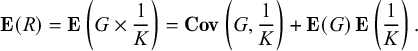 $$ \begin{align} \mathbf{E}(R) = \mathbf{E}\left(G\times\frac{1}{K}\right) = \mathbf{Cov}\left(G,\frac{1}{K}\right) + \mathbf{E}(G) \, \mathbf{E}\left(\frac{1}{K}\right). \end{align} $$
The second equality follows from the elementary formula for covariance: $\mathbf {Cov}(X,Y) = \mathbf {E}(XY)-\mathbf {E}(X)\mathbf {E}(Y)$
.
$\mathbf {Cov}(X,Y) = \mathbf {E}(XY)-\mathbf {E}(X)\mathbf {E}(Y)$
.
If the manager raises new capital only when things are going badly, then K will be larger on average when the final gain G is small or negative, and $\mathbf {Cov}(G,1/K)$
will be positive. If
$\mathbf {Cov}(G,1/K)$
will be positive. If $\mathbf {Cov}(G,1/K)$
is large enough, it can make the expected return
$\mathbf {Cov}(G,1/K)$
is large enough, it can make the expected return $\mathbf {E}(R)$
positive even when
$\mathbf {E}(R)$
positive even when $\mathbf {E}(G)$
is negative. We call anything the manager does to create or increase a positive covariance between G and
$\mathbf {E}(G)$
is negative. We call anything the manager does to create or increase a positive covariance between G and $1/K$
martingaling, and we call this covariance the martingale index. In light of the decomposition (2.2), the martingale index can be considered a measure of the portion of the expected return due to K’s randomness. We write
$1/K$
martingaling, and we call this covariance the martingale index. In light of the decomposition (2.2), the martingale index can be considered a measure of the portion of the expected return due to K’s randomness. We write $\mathbf {M}$
for the martingale index:
$\mathbf {M}$
for the martingale index:
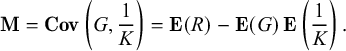 $$ \begin{align} \mathbf{M} = \mathbf{Cov}\left(G,\frac1K\right) = \mathbf{E}(R) - \mathbf{E}(G) \, \mathbf{E}\left(\frac{1}{K}\right). \end{align} $$
Like the expected return $\mathbf {E}(R)$
, the martingale index
$\mathbf {E}(R)$
, the martingale index $\mathbf {M}$
is invariant under changes in the unit of measurement: if such a change multiplies G by c, then it multiplies
$\mathbf {M}$
is invariant under changes in the unit of measurement: if such a change multiplies G by c, then it multiplies $1/K$
by
$1/K$
by $1/c$
and thus leaves all the terms in (2.2) and (2.3) unchanged.
$1/c$
and thus leaves all the terms in (2.2) and (2.3) unchanged.
These ideas and definitions apply not only to money managers but also to anyone else who is making investment or betting decisions over time, including corporate executives and other business people, as well as individuals who are betting on casino games, horses, or sports.
The expected values and covariances in (2.2) and (2.3) depend in part on vagaries of the Roulette wheel, on fluctuations in security prices, or on outcomes of the horse races or sports events. But for many martingalers they depend even more on randomness in betting choices. In many of our examples, we will think of $\mathbf {M}$
and the expected values and covariance that define it as properties of randomizing strategies hypothesized to mimic martingaling behavior.
$\mathbf {M}$
and the expected values and covariance that define it as properties of randomizing strategies hypothesized to mimic martingaling behavior.
In both (2.1) and (2.2), we assume that $G\ge -K$
. A player in a casino is not allowed to make a bet without putting on the table the amount needed to cover the greatest possible loss, and by definition, the amount a money manager risks is their greatest possible loss. It follows that
$G\ge -K$
. A player in a casino is not allowed to make a bet without putting on the table the amount needed to cover the greatest possible loss, and by definition, the amount a money manager risks is their greatest possible loss. It follows that $R\ge -1$
. If the manager’s bets are not sure losers, then
$R\ge -1$
. If the manager’s bets are not sure losers, then $\mathbf {E}(R)>-1$
. But there is no general theoretical upper bound on
$\mathbf {E}(R)>-1$
. But there is no general theoretical upper bound on $\mathbf {E}(R)$
even for the case where
$\mathbf {E}(R)$
even for the case where $\mathbf {E}(G)\leq 0$
.
$\mathbf {E}(G)\leq 0$
.
The martingaler’s time and resources being finite, the strategy that we devise to mimic the martingaler’s behavior must define an upper bound, say $\mathbf {K}$
, on the amount the martingaler could lose before running out of money and credit or simply giving up trying to recoup their losses. The martingaler usually does not know
$\mathbf {K}$
, on the amount the martingaler could lose before running out of money and credit or simply giving up trying to recoup their losses. The martingaler usually does not know $\mathbf {K}$
at the outset, and if they are lucky they will stop when they are ahead and never learn it. This is true even when the martingaler is in a casino and is trying to follow a martingale that they have been told about. Those who tout martingales do not tell you precisely how far ahead you should try to get, and they do not talk about the situation where you are so far behind that you must give up.
$\mathbf {K}$
at the outset, and if they are lucky they will stop when they are ahead and never learn it. This is true even when the martingaler is in a casino and is trying to follow a martingale that they have been told about. Those who tout martingales do not tell you precisely how far ahead you should try to get, and they do not talk about the situation where you are so far behind that you must give up.
We can distinguish between the simple return for the strategy we use to describe the martingaler’s behavior and the simple return as the martingaler sees it. The strategy’s simple return is $G/\mathbf {K}$
. But the martingaler’s simple return R is
$G/\mathbf {K}$
. But the martingaler’s simple return R is $G/K$
; this is what the martingaler sees when she stops betting. And it is
$G/K$
; this is what the martingaler sees when she stops betting. And it is $\mathbf {E}(R)$
that she might estimate by trying her martingale several times and averaging the Rs she obtains. It is
$\mathbf {E}(R)$
that she might estimate by trying her martingale several times and averaging the Rs she obtains. It is $\mathbf {E}(R)$
, the martingaler’s expected simple return that we study in this paper.
$\mathbf {E}(R)$
, the martingaler’s expected simple return that we study in this paper.
Two toy examples
To illustrate the decomposition (2.2) we now look at the martingale index for two examples, each involving just two rounds of investments.
An executive’s martingale
Consider this hypothesized model for a project in which an executive initially invests $1$
unit of capital:
$1$
unit of capital:
-
• The project chosen either produces a net gain of $1$
(probability
$1/4$
) or requires an additional investment of
$3$
(probability
$3/4$
).
$1$
(probability
$1/4$
) or requires an additional investment of
$3$
(probability
$3/4$
). -
• With the additional investment, the project finally produces either a net gain of
$1$
(probability
$2/3$
) or a loss of the entire investment (probability
$1/3$
).


No executive would deliberately follow such a strategy, and it would never be possible to justify such precise probabilities. But when deciding whether to undertake a project, corporations often conjecture more favorable probabilities that turn out to be unrealistic. The executive who makes the initial investment in our imagined project may believe, on the basis of misleading and perhaps random information, that immediate success without further investment is almost guaranteed.
In any case, the pair $(K,G)$
has this joint distribution under the hypothesized model:
$(K,G)$
has this joint distribution under the hypothesized model:
-
• with probability
$1/4$
,
$K=1$
and
$G=1$
, and hence
$R=1$
, -
• with probability
$1/2$
,
$K=4$
and
$G=1$
, and hence
$R=1/4$
, -
• with probability
$1/4$
,
$K=4$
and
$G=-4$
, and hence
$R=-1$
.


We see that $\mathbf {K}=4$
, and we find
$\mathbf {K}=4$
, and we find
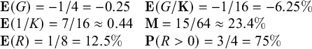 $$\begin{align*}\begin{array}{lll} \mathbf{E}(G)=-1/4 = -0.25 && \mathbf{E}(G/\mathbf{K})=-1/16 = -6.25\% \\ \mathbf{E}(1/K)=7/16 \approx 0.44 && \mathbf{M} = 15/64 \approx 23.4\%\\ \mathbf{E}(R)=1/8 =12.5\% &&\mathbf{P}(R>0)=3/4 =75\% \end{array} \end{align*}$$
In spite of the strategy’s negative expected gain, the martingaler’s expected return, $\mathbf {E}(R)$
, and the martingaler’s probability of a positive return,
$\mathbf {E}(R)$
, and the martingaler’s probability of a positive return, $\mathbf {P}(R>0)$
, are favorable.
$\mathbf {P}(R>0)$
, are favorable.
The point of this example is that a positive return over a sequence of projects that will likely have cost overruns is not good evidence for an ability to choose projects with a positive expected gain. The martingale index of more than 20% can help make this elementary point vivid to students and even to corporate boards.
An entrepreneur’s paroli
Rather than betting more when you lose, you can bet more when you win, using the winnings from your bet to do so. A system that does this was called a paroli. If you win several consecutive rounds while reinvesting your winnings, you will multiply the money you initially put on the table by a great deal, but the probability of achieving this is small. A paroli seems to be the opposite of a martingale. It risks a little in return for a small probability of a large gain, as opposed to risking a lot in return for a high probability of a small gain. But if you try a paroli and lose, it is tempting to try again and to keep trying until you achieve the gain you were aiming for. Then you are martingaling.
A more extreme paroli will not only reinvest winnings but add more capital following each win. This can produce a negative martingale index. Consider, for example, this hypothesized model for an entrepreneur’s use of capital:
-
• The entrepreneur first chooses a project in which to invest
$1$
. Half the projects in which she might invest would produce a net gain of
$1$
; the other half would result in loss of the investment. She cannot tell the two classes of investments apart, so she chooses randomly. With probability
$1/2$
, she chooses a project that produces the gain of
$1$
; with probability
$1/2$
, she chooses a project that loses her investment. -
• If the project produces a net gain, the entrepreneur raises additional capital of
$2$
to invest along with the
$2$
already on the table (the initial investment of
$1$
and the additional
$1$
gained). She uses this total capital of 4 for a new project but again must choose randomly between projects. In this case she has probability
$1/4$
of choosing a project that returns
$15$
, for an overall net gain of
$12$
, and probability
$3/4$
of choosing a project that loses the whole investment.


Here $(K,G)$
has this joint distribution:
$(K,G)$
has this joint distribution:
-
• with probability
$1/2$
,
$K=1$
and
$G=-1$
, and hence
$R=-1$
, -
• with probability
$3/8$
,
$K=3$
and
$G=-3$
, and hence
$R=-1$
, -
• with probability
$1/8$
,
$K=3$
and
$G=12$
, and hence
$R=4$
.


We see that $\mathbf {K}=3$
, and we find
$\mathbf {K}=3$
, and we find
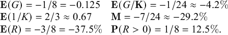 $$\begin{align*}\begin{array}{lll} \mathbf{E}(G)=-1/8 = -0.125 && \mathbf{E}(G/\mathbf{K})=-1/24 \approx -4.2\% \\ \mathbf{E}(1/K)=2/3 \approx 0.67 && \mathbf{M} = -7/24 \approx -29.2\%\\ \mathbf{E}(R)=-3/8 =-37.5\% &&\mathbf{P}(R>0)=1/8 =12.5\%. \end{array} \end{align*}$$
This paroli has a negative martingale index because it puts more money on the table when it wins. The size of the negative martingale index signals that most of the large negative expected return is due to this randomness in the total investment.
Multiplying your money by $4$
is spectacular. If the entrepreneur has backers with deep pockets, who can tolerate a string of failures before she succeeds, this startling level of success may obscure the memory of how much they may have previously lost.
$4$
is spectacular. If the entrepreneur has backers with deep pockets, who can tolerate a string of failures before she succeeds, this startling level of success may obscure the memory of how much they may have previously lost.
3. The martingale index in the casino
Casinos provide the most striking examples of the seductiveness of martingales, for several reasons. First, we do not need to invent hypothetical probability distributions in order to analyze the martingaling. There are well known and reliable probabilities for red and black. Second, these probabilities favor the casino, and so the martingaler seems to be beating the odds. Third, the typical bets, at least those that attracted martingalers in the classical casinos, are all-or-nothing even-money bets. You bet on red or black, and you either lose what you bet or double your money. This all-or-nothing betting, as we will see, can produce very large martingale indexes and expected returns.
When we turn to the stock market in §4, we will see more modest martingale indexes and expected returns. This might give the impression that our study of the casino exaggerates the dangers martingalers face in the 21st century. But the story of the casino is being reproduced by the current craze for online sports betting. Unlike the stock market, where outcomes are less extreme, and the racetrack or the lottery, where most bets risk small amounts for large payoffs, much betting on sports is all-or-nothing and approximately even-money. You lose your money if the team you bet on loses, and you may approximately double your money if it wins. And the sports arena can be even more seductive than the casino, because of the greater role of emotion, and because of the huge amount of information that can tempt you to think that you have insights others do not have.
Returning to the casino, where probabilities and expected values are objective and known, recall that a bet in which you pay c and get a random amount H in return is said to be fair if $\mathbf {E}(H)=c$
, advantageous if
$\mathbf {E}(H)=c$
, advantageous if $\mathbf {E}(H)>c$
, and disadvantageous if
$\mathbf {E}(H)>c$
, and disadvantageous if $\mathbf {E}(H)<c$
. If
$\mathbf {E}(H)<c$
. If
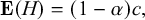 $$ \begin{align} \mathbf{E}(H)=(1-\alpha)c, \end{align} $$
then we call $\alpha $
the house’s advantage. It is the fraction of the money put on the table that the house takes in the long run when the bet is repeated. The gambler’s gain G being
$\alpha $
the house’s advantage. It is the fraction of the money put on the table that the house takes in the long run when the bet is repeated. The gambler’s gain G being $H-c$
, we see that
$H-c$
, we see that $\mathbf {E}(G/c)=-\alpha $
. In words: the expected return on the bet is minus the house’s advantage.
$\mathbf {E}(G/c)=-\alpha $
. In words: the expected return on the bet is minus the house’s advantage.
As we just mentioned, the casino martingales we will discuss use only even-money bets—i.e., bets in which you win or lose some fixed amount c. This means that you pay c for a random amount H that is equal to either $2c$
or
$2c$
or $0$
. If the probability of winning is p, then
$0$
. If the probability of winning is p, then $\mathbf {E}(H)=2c p$
. Comparing this with (3.1), we see that
$\mathbf {E}(H)=2c p$
. Comparing this with (3.1), we see that $\alpha $
and p are related by
$\alpha $
and p are related by
 $$\begin{align*}(1-\alpha)=2p, \quad \text{or} \quad p = \frac{1-\alpha}{2}. \end{align*}$$
The classical casino games are disadvantageous to the player; $\alpha>0$
. But we will also consider fair (
$\alpha>0$
. But we will also consider fair ( $\alpha =0$
) and advantageous (
$\alpha =0$
) and advantageous ( $\alpha <0$
) bets, because these may arise in financial settings.
$\alpha <0$
) bets, because these may arise in financial settings.
Three values of $\alpha $
are particularly relevant to the classical casino games:
$\alpha $
are particularly relevant to the classical casino games:
-
•
$\alpha = 0.01$
, approximately the house advantage in Trente et Quarante, the classical casino game least disadvantageous to the player, -
•
$\alpha = 1/37\approx 0.027027027$
, the house advantage in European Roulette, -
•
$\alpha = 2/38\approx 0.052631579$
, the house advantage in American Roulette.


Play can be very fast; in Roulette you might be able to play 600 rounds in a day. But some of the strategies we mention cannot be implemented because of the casino’s limit on the size of a bet. This limit was typically no more than 100 times the minimum bet in the early 19th century, and no more than 1,000 times in the late 20th century.
The classical martingales that we consider in this section become fully defined strategies only when we specify a stopping rule. One attractive stopping rule, obvious but hard to implement, is to stop when you are ahead. Doing this precisely—i.e., setting a goal and really stopping if and when you achieve it or run out of money—is enough to create a mild martingale, because stopping after you win is a way of betting less after winning.
As we mentioned in the introduction, classical martingales varied not only the amount bet but also the color bet on. The rules for how much to bet were called the massage; the rules for choosing between red and black were called the attaque (Shafer, Reference Shafer, Mazliak and Shafer2022, p. 45). The attaque sometimes specified the choice as a function of preceding outcomes, but often the player was advised to rely on their intuition. In either case, we could say that their choice was random, and we know that it did not affect the chances of winning or losing. Because the choice of color makes no difference in the probabilities, we will ignore it here.
We begin our exploration of casino martingales, in §3.1, by studying the martingale index for a strategy that keeps its bet size constant and stops either when it achieves a specified modest gain or after some specified number of bets. In §3.2, we consider the classical martingale, which doubles its bets after every loss, up to some limit. In §3.3, we consider a more subtle martingale, the d’Alembert. Also called the gradual martingale, it was probably the most popular martingale in the 19th century; with the right stopping rule, it achieves a positive expected return with very high probability while disguising its potential for large losses.
Many other casino martingales have been tried, advertised, and deplored. For details on these martingales and the casino games in which they were played, see Ethier (Reference Ethier2010) and Shafer (Reference Shafer, Mazliak and Shafer2022) and the references therein.
3.1. Constant bets
The simplest way to gamble in the casino is to make the same even-money bet over and over. The resulting cumulative gain is a random walk, as in Figure 1. The past century produced an immense literature on the random walk, but we consider only some very simple points, most already understood by the draftsman who produced Figure 1 two centuries ago.
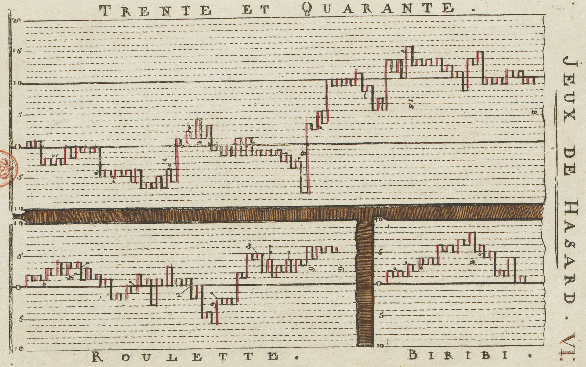
Figure 1 Random walk in the casino.
Note: Cumulative excess of red over black observed in plays of three casino games, published by Jacques-Joseph Boreux (1755–1846) in 1820 (Smyll, Reference Smyll1820, Plate VI). This is probably the first graph of a random walk ever published. Source: Bibliothèque nationale de France.
A simple stopping rule is to stop when you reach a certain goal, say g, for your gain G. We will emphasize the case where g is $3$
or less. Many gamblers will take it for granted that this goal will be reached very soon. But in fact there is a non-negligible probability that it will not be reached after hundreds of rounds. So we need to set a limit on the number of rounds, say
$3$
or less. Many gamblers will take it for granted that this goal will be reached very soon. But in fact there is a non-negligible probability that it will not be reached after hundreds of rounds. So we need to set a limit on the number of rounds, say $N_{\text {max}}$
. Our rule, then, is to play until G is first equal to g or
$N_{\text {max}}$
. Our rule, then, is to play until G is first equal to g or $N_{\text {max}}$
rounds, whichever is sooner.
$N_{\text {max}}$
rounds, whichever is sooner.
Table 1 and Figures 2 and 3 provide some detail on what such strategies can achieve. We obtain the most impressive results with the very modest goal of $g=1$
. We see from Table 1 that when
$g=1$
. We see from Table 1 that when $g=1$
and
$g=1$
and $N_{\text {max}}=50$
, the probability of a positive return is above
$N_{\text {max}}=50$
, the probability of a positive return is above $80\%$
for Roulette and Trente et Quarante, and the expected return is substantial even when the house advantage is
$80\%$
for Roulette and Trente et Quarante, and the expected return is substantial even when the house advantage is $20\%$
. The greater probability of success for the smallest goal g echoes a cliché of 19th century martingalers (Shafer, Reference Shafer, Mazliak and Shafer2022, p. 28): limit your martingale, settle for small gains.
$20\%$
. The greater probability of success for the smallest goal g echoes a cliché of 19th century martingalers (Shafer, Reference Shafer, Mazliak and Shafer2022, p. 28): limit your martingale, settle for small gains.
Table 1 Constant betting for $50$
rounds
$50$
rounds
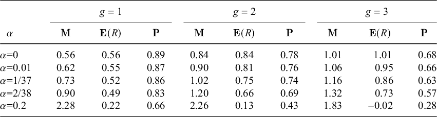
Note: Estimated martingale index $\mathbf {M}$
, expected return
$\mathbf {M}$
, expected return $\mathbf {E}(R)$
, and probability of a positive return
$\mathbf {E}(R)$
, and probability of a positive return $\mathbf {P}=\mathbf {P}(R>0)$
for several values of the house advantage
$\mathbf {P}=\mathbf {P}(R>0)$
for several values of the house advantage $\alpha $
and the goal g for constant betting and
$\alpha $
and the goal g for constant betting and $N_{\text {max}}=50$
. Estimates are based on one million replications and rounded to two significant figures. (By definition,
$N_{\text {max}}=50$
. Estimates are based on one million replications and rounded to two significant figures. (By definition, $\mathbf {M}=\mathbf {E}(R)$
when
$\mathbf {M}=\mathbf {E}(R)$
when $\alpha =0$
.)
$\alpha =0$
.)
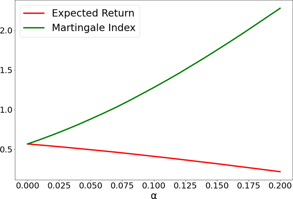
Figure 2 Constant bets: Effect of house’s advantage.
Note: Expected return and martingale index as functions of the house’s advantage $\alpha $
when you stop when you are
$\alpha $
when you stop when you are $1$
unit ahead or after
$1$
unit ahead or after $50$
bets, whichever happens first.
$50$
bets, whichever happens first.
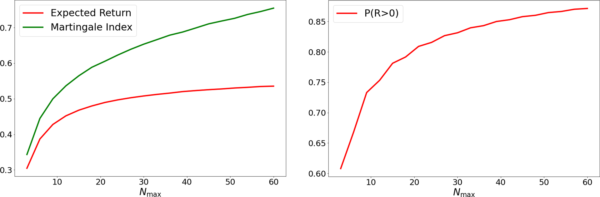
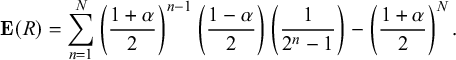
Figure 3 Constant betting in European Roulette, where the house advantage is $1/37$
.
$1/37$
.
Note: Expected return, martingale index, and probability of positive return as functions of the maximum number of bets $N_{\text {max}} $
when you stop as soon as you are
$N_{\text {max}} $
when you stop as soon as you are $1$
unit ahead.
$1$
unit ahead.
Figure 2 shows the rapid growth of the martingale index and the corresponding slow decline of the expected return as $\alpha $
increases. Increasing
$\alpha $
increases. Increasing $\alpha $
gives a greater probability to the cases where G has a large negative value and K is large, thus increasing
$\alpha $
gives a greater probability to the cases where G has a large negative value and K is large, thus increasing $\mathbf {M}$
, their covariance. This effect, together with the decrease in
$\mathbf {M}$
, their covariance. This effect, together with the decrease in $\mathbf {E}(1/K)$
in the second term of (2.2), makes
$\mathbf {E}(1/K)$
in the second term of (2.2), makes $\mathbf {E}(R)$
less sensitive to
$\mathbf {E}(R)$
less sensitive to $\alpha $
than we might at first expect.
$\alpha $
than we might at first expect.
Figure 3 shows how $\mathbf {E}(R)$
,
$\mathbf {E}(R)$
, $\mathbf {M}$
, and
$\mathbf {M}$
, and $\mathbf {P}(R>0)$
vary with
$\mathbf {P}(R>0)$
vary with $N_{\text {max}}$
for
$N_{\text {max}}$
for $g=1$
and the house advantage in European Roulette,
$g=1$
and the house advantage in European Roulette, $\alpha =1/37\approx 0.027$
. We see that
$\alpha =1/37\approx 0.027$
. We see that $\mathbf {E}(R)$
and
$\mathbf {E}(R)$
and $\mathbf {P}(R>0)$
do not increase very quickly after the first
$\mathbf {P}(R>0)$
do not increase very quickly after the first $20$
rounds.
$20$
rounds.
Most gamblers who set out to bet until they are $1$
ahead have not done these calculations and do not think they will ever need to bet
$1$
ahead have not done these calculations and do not think they will ever need to bet $50$
or
$50$
or $60$
times, being overly optimistic about how soon they can expect the recover from an initial loss.Footnote
2
But the probabilities
$60$
times, being overly optimistic about how soon they can expect the recover from an initial loss.Footnote
2
But the probabilities $\mathbf {P}(R>0)$
in Table 1 are not high enough to sustain belief in the strategy very long. Even if she maintains the discipline to stop when only
$\mathbf {P}(R>0)$
in Table 1 are not high enough to sustain belief in the strategy very long. Even if she maintains the discipline to stop when only $1$
ahead, a gambler is likely to have an unpleasant surprise relatively soon when she tries the strategy several times. If she tries it
$1$
ahead, a gambler is likely to have an unpleasant surprise relatively soon when she tries the strategy several times. If she tries it $5$
times in European roulette, it is more likely than not that she will be behind after
$5$
times in European roulette, it is more likely than not that she will be behind after $50$
bets at least once;
$50$
bets at least once; $(0.86)^5\approx 0.47$
. As we will see in §3.3, the d’Alembert lends itself better to self-deception.
$(0.86)^5\approx 0.47$
. As we will see in §3.3, the d’Alembert lends itself better to self-deception.
3.2. The classic martingale
Double your bet when you lose. This betting strategy, no doubt as ancient as money, was the first to be called a martingale (Shafer, Reference Shafer, Mazliak and Shafer2022). We call it the classic martingale. It has a positive martingale index.
We may assume that you begin by betting $1$
, and it is implicit that you stop as soon as you win, but to fully define the strategy we must specify a number of rounds, say N, after which you stop even if you have not yet won. If N is reasonably large, then you are almost certain to win; you lose only with the very small probability
$1$
, and it is implicit that you stop as soon as you win, but to fully define the strategy we must specify a number of rounds, say N, after which you stop even if you have not yet won. If N is reasonably large, then you are almost certain to win; you lose only with the very small probability
 $$\begin{align*}\left(\frac{1+\alpha}{2}\right)^N. \end{align*}$$
But if you lose on all N rounds, you lose
 $$\begin{align*}1+2+2^2+\cdots 2^{N-1} = 2^N -1, \end{align*}$$
which is very large even for modest values of N. As $2^{10} -1 = 1023$
, the strategy cannot be implemented for
$2^{10} -1 = 1023$
, the strategy cannot be implemented for $N=10$
in a casino that limits the size of a bet to 1,000 times the minimum bet.
$N=10$
in a casino that limits the size of a bet to 1,000 times the minimum bet.
When you do win, you win only $1$
; if you lose n rounds, where
$1$
; if you lose n rounds, where $0\le n \le N-1$
, and then win on round
$0\le n \le N-1$
, and then win on round $n+1$
, your net gain G is
$n+1$
, your net gain G is
 $$\begin{align*}G = 2^{n} - (1+2+2^2+\cdots 2^{n-1}) =1. \end{align*}$$
So the argument that the strategy is almost sure to win can lure only the most gullible into the casino.
The expected net gain is of course zero if $\alpha =0$
and negative otherwise:
$\alpha =0$
and negative otherwise:
 $$ \begin{align} \mathbf{E}(G) = \left(1- \left(\frac{1+\alpha}{2}\right)^N\right) -\left(\frac{1+\alpha}{2}\right)^N (2^N-1) = 1 - (1+\alpha)^N. \end{align} $$
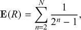
The expected return is
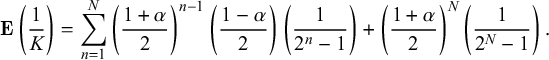
 $$ \begin{align} \mathbf{E}(R) = \sum_{n=1}^{N} \left(\frac{1+\alpha}{2}\right)^{n-1}\left(\frac{1-\alpha}{2}\right) \left( \frac{1}{2^n-1}\right) - \left(\frac{1+\alpha}{2}\right)^N. \end{align} $$
When $\alpha =0$
, (3.3) reduces to
$\alpha =0$
, (3.3) reduces to
 $$\begin{align*}\mathbf{E}(R) = \sum_{n=2}^N \frac{1}{2^{n}-1}, \end{align*}$$
which is equal, to two significant figures, to $0.61$
when
$0.61$
when $N>9$
. In general, (3.3) is positive except when
$N>9$
. In general, (3.3) is positive except when $N=1$
or
$N=1$
or $\alpha $
is very large; see Table 2.
$\alpha $
is very large; see Table 2.
Table 2 House advantages for which the classic martingale has a positive expected return
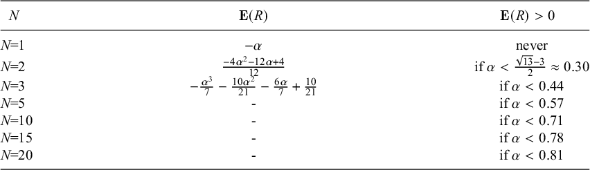
Note: The right-hand column identifies the values of $\alpha $
for which (3.3) is positive.
$\alpha $
for which (3.3) is positive.
We can also write a formula for $\mathbf {E}(1/K)$
:
$\mathbf {E}(1/K)$
:
 $$ \begin{align} \mathbf{E}\left( \frac1K \right) = \sum_{n=1}^{N} \left(\frac{1+\alpha}{2}\right)^{n-1}\left(\frac{1-\alpha}{2}\right) \left( \frac{1}{2^n-1}\right) + \left(\frac{1+\alpha}{2}\right)^N \left( \frac{1}{2^N-1}\right). \end{align} $$
The martingale index can be computed from (3.2), (3.3), and (3.4). It is positive when $N>1$
.
$N>1$
.
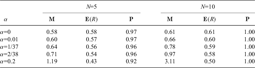
Figure 4 and Table 3, illustrate how the properties of the classic martingale are affected by the house’s advantage. We see that the extent to which even large house advantages dampen $\mathbf {E}(R)$
and
$\mathbf {E}(R)$
and $\mathbf {P}(R>0)$
is surprisingly slight. The increasingly deceptive character of
$\mathbf {P}(R>0)$
is surprisingly slight. The increasingly deceptive character of $\mathbf {E}(R)$
and
$\mathbf {E}(R)$
and $\mathbf {P}(R>0)$
is measured, we might say, by the increasing value of the martingale index. This is consistent with the pattern we saw for constant bets.
$\mathbf {P}(R>0)$
is measured, we might say, by the increasing value of the martingale index. This is consistent with the pattern we saw for constant bets.
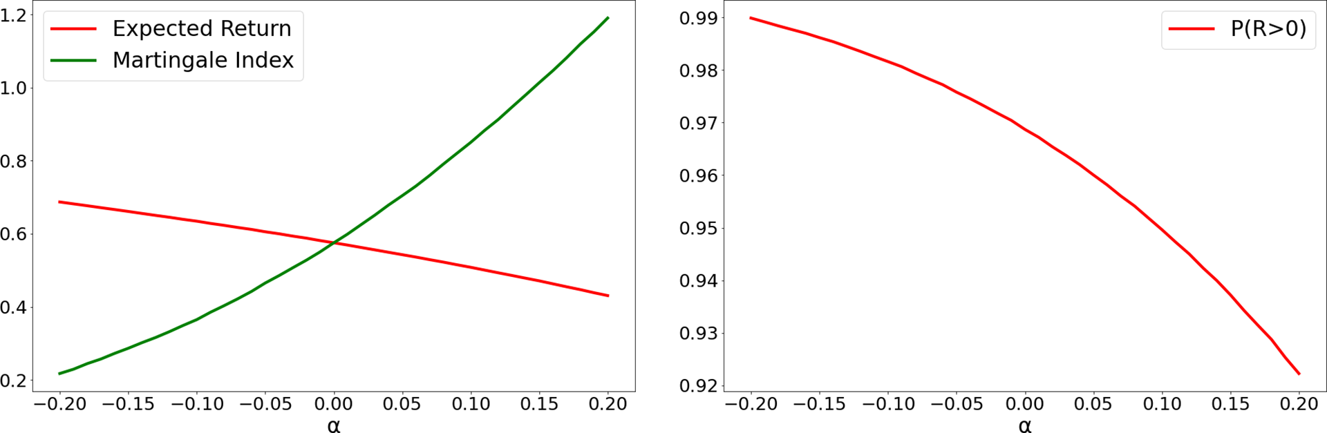
Figure 4 The classic martingale: expected return, martingale index, and probability of positive return for $N=5$
$N=5$
Table 3 Performance of the classic martingale
Note: $\mathbf {P}=\mathbf {P}(R>0)$
. Estimates are based on two million replications and rounded to two significant figures.
$\mathbf {P}=\mathbf {P}(R>0)$
. Estimates are based on two million replications and rounded to two significant figures.
While the classic martingale gives the gambler a much greater chance of winning than the strategy of constant bets, its obvious potential for huge losses limits its attractiveness. It is typically the resort of the desperate, who have blundered into a loss already too large to digest while believing that they were playing safer strategies. But if they resort to it a few times and succeed each time, they may be tempted into even wilder play. Nick Leeson, the trader who brought down Barings Bank in 1995, was in the habit of extracting himself from disasters by repeatedly doubling his bet before he turned to outright fraud (Fay, Reference Fay1996).
3.3. The d’Alembert
The history of the d’Alembert is recounted by Shafer (Reference Shafer, Mazliak and Shafer2022) and compared to other popular casino martingales by Crane and Shafer (Reference Crane and Shafer2020). It was sometimes called the gradual martingale. Like the classical martingale, it delivers a small gain with high probability. But it does so in a gradual way that disguises the danger of large losses. We single it out here from the multitude of 19th-century casino martingales because it was so notorious for its ability to seduce. If you set a modest goal, say a gain of only one or two or three units, you are very likely to experience an amazing string of successes before you encounter a disaster.
To play the d’Alembert you first bet $1$
and then, on successive rounds:
$1$
and then, on successive rounds:
-
• if you lose, increase your bet by one unit, and
-
• if you win, decrease your bet by one unit unless it is already one unit.
To make it a strategy, we must specify a stopping rule. As with the constant bet, it is natural to use a rule that stops after reaching some goal g for the gain or after $N_{\text {max}}$
bets, whichever comes first.
$N_{\text {max}}$
bets, whichever comes first.
Hawkers who used the strategy to attract players into their casino often suggested that the player stop when they are a few units ahead, and the chances are high for this happening fairly quickly the first few times the strategy is tried. For players who fancied themselves mathematicians, a hawker might suggest that when they lose they should keep playing until the number of wins and losses equalizes; everyone knows that this will happen eventually and then the player will then be ahead by the number of wins. See Ethier (Reference Ethier2010, pp. 289–292) for a proof. The expectation that the wins and losses will equalize can be compared with the equilibrium in physics explained by ‘d’Alembert’s principle’; thus the name ‘d’Alembert’s martingale.’ There is no evidence that the famous savant Jean Le Rond d’Alembert ever encountered or used the d’Alembert.
Figure 5 and Table 4 give some quantitative details on the d’Alembert. The system’s very high probability of success is, of course, the key to its seductiveness. In the case of Trente et Quarante, according to Table 4, the probability of a positive return with $N_{\text {max}}=50$
and
$N_{\text {max}}=50$
and $g=2$
is approximately
$g=2$
is approximately $0.97$
, so that the probability of winning each time if you try it five times is approximately
$0.97$
, so that the probability of winning each time if you try it five times is approximately $(0.97)^5\approx 0.86$
. As the expected returns indicate, the five wins usually would not require taking very much out of one’s pocket. Many a novice found their initial success convincing evidence that they had found either the key to beating the odds or else a durable streak of good luck.
$(0.97)^5\approx 0.86$
. As the expected returns indicate, the five wins usually would not require taking very much out of one’s pocket. Many a novice found their initial success convincing evidence that they had found either the key to beating the odds or else a durable streak of good luck.
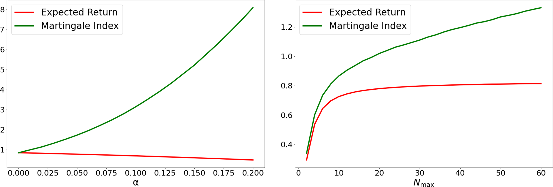
Figure 5 The d’Alembert with $g=2$
. On the left,
$g=2$
. On the left, $N_{\text {max}}=50$
and
$N_{\text {max}}=50$
and $\alpha $
varies.
$\alpha $
varies.
Note: On the right, $\alpha =1/37$
and
$\alpha =1/37$
and $N_{\text {max}}$
varies.
$N_{\text {max}}$
varies.
Table 4 Performance of the d’Alembert with $N_{\text {max}}=50$

Note: Estimates based on 100,000 replications and rounded to two decimals.
4. The martingale index in finance
A player in a casino can bet on red or black. A trader in a financial market can bet on a given security’s price going up or down. Both can martingale by betting more when they are losing. But a trader who takes a position in financial securities may gain or lose many different amounts, and they seldom win or lose all they risk. This slows down martingaling, because a longer sequence of bets may be needed in order to create the risk of a large loss. The martingale indexes that we will find using financial instruments are one or two orders of magnitudes smaller than those we found in the casino.
Many financial markets offer the possibility of trading on margin, however, making it easier to take large risks quickly. Margin calls are invitations to martingale; they call on the trader whose position is losing value to add more capital merely to maintain their position.
Financial markets also differ from casinos in the opportunity the trader has to base trading decisions on extensive information. One spin of the Roulette wheel follows the next very quickly; the player has no time to gather information and calculate. The d’Alembert’s popularity derived in part from its simplicity: your bet depended only on the previous round: how much you had bet and whether the bet had won or lost. Traders, in contrast—even high-frequency traders—have access to an immense amount of information about the economy and about the securities they are trading, as well as the time and resources to use it. This only increases the possibilities for self-delusion. The more information you have, the more plausibly you can attribute momentary success to having interpreted some particular information more wisely than other market participants.
Another difference between the casino and a financial market is that a market’s randomness is not well defined. In a respectable casino, the probabilities are usually known and undisputed. In a financial market, probabilities are only hypothetical. Scholars and sophisticated traders have invented probability models for the movement of prices, but these are only models, and skeptics can always argue that an unwelcome implication of a model represents a point of difference between the model and the reality modeled. In general, such market models are especially unreliable as predictors of extreme events, precisely the ones that often inflict the greatest losses on martingalers.
As we explained in the introduction, we model the trader rather than the market. For simplicity and to avoid modeling the market, we use the historical record of returns for the financial instruments we consider. We randomize these returns to create hypothetical price trajectories. We do not use information from outside the market, but we incorporate the idea that the trader is acting on irrelevant information by assuming that they are choosing trades randomly. The resulting models are not realistic as hypotheses about the behavior and experience of any particular trader, but they allow us to illustrate the possible results of martingaling.
In this section, we give examples of martingaling by a fictitious trader whom we call Jane. In §4.1, Jane bets every day on whether the S&P 500 index will go up or down that day. She does this by taking a position on margin in S&P 500 futures. Part of her martingaling is simply meeting margin calls. But she also uses her cumulative performance so far when deciding on the size of each bet, betting more when behind and less when ahead.
In §4.2, Jane tries to beat the S&P 500 index by picking each day an individual stock that she thinks will do better than the index that day. In this example, she does not trade on margin, but she still martingales by betting more when behind, betting less when ahead, and trying to stop when ahead.
4.1. Betting on the ups and downs of the S&P 500
One of the most popular futures products is the Chicago Mercantile Exchange’s E-mini futures on the S&P 500 index. Contracts in this market are issued four times a year. At expiration, each contract is worth $50$
times the current value of the S&P 500 index. So
$50$
times the current value of the S&P 500 index. So $(1/50)$
th of the current price of the contract is called the ‘futures price.’ A trader can go long or short in a contract. For the contract closest to expiration, the ‘front contract,’ the futures price is usually very close to the index. The contracts trade nearly
$(1/50)$
th of the current price of the contract is called the ‘futures price.’ A trader can go long or short in a contract. For the contract closest to expiration, the ‘front contract,’ the futures price is usually very close to the index. The contracts trade nearly $24$
hours a day from
$24$
hours a day from $6$
pm Sunday to
$6$
pm Sunday to $5$
pm Friday, New York time. The market is closed each trading day between
$5$
pm Friday, New York time. The market is closed each trading day between $5$
pm and
$5$
pm and $6$
pm, while a settlement price is calculated and posted.
$6$
pm, while a settlement price is calculated and posted.
To study martingaling in the S&P 500 E-mini, we use daily data on the front contract provided by Refinitiv for the 24 years 1998 through 2021.Footnote 3 These data include the contract’s opening price, highest price, lowest price, and settlement price for each day, as well as the trading volume and the number of open contracts. Approximately 54% of the returns calculated from these data are positive. Table 5 provides some summary statistics.
Table 5 Average daily behavior of the S&P 500 E-mini for the 6,050 trading days from 1998 through 2021
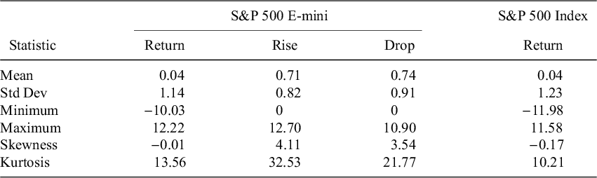
Note: Return = 100(S $-$
O)/O, drop = 100(0
$-$
O)/O, drop = 100(0 $-$
L)/O, and rise = 100(H
$-$
L)/O, and rise = 100(H $-$
O)/O, where O, L, H, and S are the opening, low, high, and settlement prices for the day. Statistics on the S&P 500’s returns for the same 24 years (in this case, the return is the percent change from one day’s closing to the next) are included for comparison.
$-$
O)/O, where O, L, H, and S are the opening, low, high, and settlement prices for the day. Statistics on the S&P 500’s returns for the same 24 years (in this case, the return is the percent change from one day’s closing to the next) are included for comparison.
We construct a hypothetical probability distribution for a year-long sequence of daily futures prices $F_0,\dots ,F_{252}$
by sampling from the
$F_0,\dots ,F_{252}$
by sampling from the $6{,}050$
returns: we sample
$6{,}050$
returns: we sample $252$
returns
$252$
returns $R_1,\dots ,R_{252}$
without replacement, and we set
$R_1,\dots ,R_{252}$
without replacement, and we set $F_0=1$
and
$F_0=1$
and $F_n=F_{n-1}(1+R_n)$
for
$F_n=F_{n-1}(1+R_n)$
for $n=1,\dots ,252$
.
$n=1,\dots ,252$
.
We assume that Jane predicts at the beginning of each trading day whether the futures price will go up or down and then bets on her prediction by going long or short. She takes this position at $6$
pm when the market opens and closes it at the settlement price at
$6$
pm when the market opens and closes it at the settlement price at $5$
pm when the market closes the next day. She thinks her predictions are based on insights others do not have. But they are actually random: she goes long with probability one-half and short with probability one-half. She will lose money on average, because the futures prices go up more often than down. But she can achieve an impressive positive expected return.
$5$
pm when the market closes the next day. She thinks her predictions are based on insights others do not have. But they are actually random: she goes long with probability one-half and short with probability one-half. She will lose money on average, because the futures prices go up more often than down. But she can achieve an impressive positive expected return.
Only members of the Chicago Mercantile Exchange trade directly on the exchange. Most individuals trade through brokers, on margin. They pay into their account with the broker (called their margin account) a fraction of the value of each contract in which they take a long or short position. Margin requirements vary from broker to broker and change from time to time in response to changes in the level and volatility of the index. We must distinguish between the maintenance margin and the initial margin.
The maintenance margin, required for keeping a long or short position in a contract open is typically about five times whatever the futures price is at the moment, or one-tenth the price of a contract. The initial margin, which is required when the position is opened, is typically $10\%$
higher. We will assume that Jane’s broker requires a maintenance margin that is
$10\%$
higher. We will assume that Jane’s broker requires a maintenance margin that is $5$
times the current futures price and an initial margin
$5$
times the current futures price and an initial margin $5.5$
times the opening price.
$5.5$
times the opening price.
This arrangement magnifies the amount Jane can win or lose on her investment. If she goes long one contract, for example, she is investing only about $10\%$
of its value. The broker is loaning her the rest. If the value of the contract has gone up
$10\%$
of its value. The broker is loaning her the rest. If the value of the contract has gone up $5\%$
by the middle of the day, she has made a
$5\%$
by the middle of the day, she has made a $50\%$
profit. If it goes down, she has lost half her money, which the broker has duly taken out of her account. The loss means that she needs to add money to the account in order meet the maintenance requirement, because the contract is still worth
$50\%$
profit. If it goes down, she has lost half her money, which the broker has duly taken out of her account. The loss means that she needs to add money to the account in order meet the maintenance requirement, because the contract is still worth $95\%$
of its initial value.
$95\%$
of its initial value.
As the futures price changes during the trading day, the value of Jane’s long or short position is continuously marked to market, the gain or loss being added to or subtracted from her margin account. As soon as she is no longer meeting the maintenance margin, she receives a ‘margin call’ from the broker, asking her to add money to bring her account up to the maintenance margin. If she fails to do so promptly, the broker closes the position and her account, refunding to her whatever money remains. The initial margin provides a cushion; the broker makes the margin call only when that cushion is exhausted.Footnote 4
We consider two possibilities: (1) Jane limits her bet to just one contract each day and (2) she martingales more, taking larger positions when behind and smaller positions when ahead. In both cases, she stops when she has attained a given goal for her return or after 252 days, whichever comes first.
4.1.1. Martingaling with one contract
Here we assume that Jane limits her position each trading day, whether it be long or short, to just one contract. She closes the position at the settlement price at the end of each day, and she takes her next day’s position at the opening price. This always being a newly taken position, she adds to her margin account if necessary to make sure it meets the broker’s initial margin requirement for that day.Footnote 5 Because the data gives the maximum drop and the maximum rise of the futures price during each trading day, we can compute the total amount Jane needs to add to keep the maintenance margin in her account throughout the trading day, and we assume that she adds only this much. We assume that she does not withdraw any money from the account until she has stopped trading for the year.
We are ignoring interest on the loan being made by the broker and other transaction fees, but our scenario is a reasonable approximation to what could be done in practice,
Table 6 shows what happens on average when Jane stops when she has achieved a return of at least $20\%$
or after 252 trading days, whichever comes first. With this stopping rule, she has a positive return
$20\%$
or after 252 trading days, whichever comes first. With this stopping rule, she has a positive return $83\%$
of the time; she stops on average after
$83\%$
of the time; she stops on average after $73$
days. Her expected return is
$73$
days. Her expected return is $15\%$
. Figure 6 shows the bimodal distribution of returns: a large mode above
$15\%$
. Figure 6 shows the bimodal distribution of returns: a large mode above $20\%$
and a smaller mode below
$20\%$
and a smaller mode below $-60\%$
.
$-60\%$
.
Table 6 Randomly betting on or against the S&P 500 using E-minis
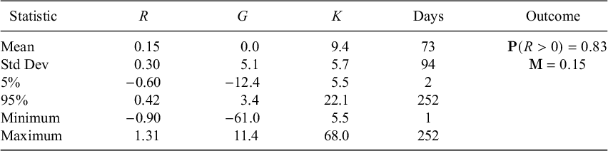
Note: Jane randomly goes long or short in one E-mini S&P 500 futures contract for up to 252 trading days, stopping early if and when she achieves a $20\%$
overall return. The estimates here are based on from 1,000,000 replications, where returns are sampled from the 6,050 historical returns. The martingaling effect comes partly from her stopping when she is ahead, partly from her need to bolster her margin account when she falls behind. On average, she increases her initial investment of 5.5–9.4.
$20\%$
overall return. The estimates here are based on from 1,000,000 replications, where returns are sampled from the 6,050 historical returns. The martingaling effect comes partly from her stopping when she is ahead, partly from her need to bolster her margin account when she falls behind. On average, she increases her initial investment of 5.5–9.4.
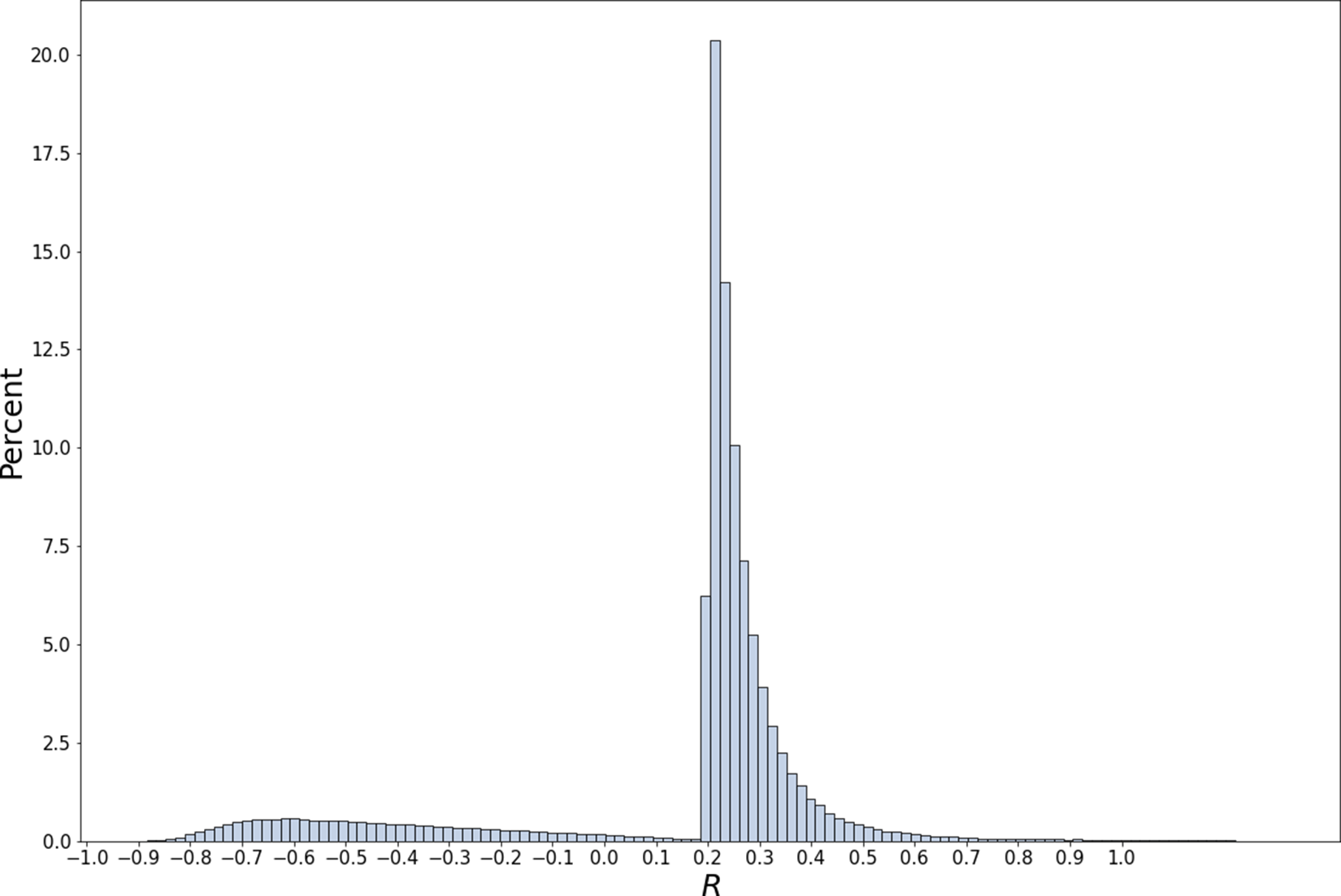
Figure 6 You go long or short on one contract for up to 252 trading days, stopping as soon as you have a $20\%$
overall return.
$20\%$
overall return.
Note: See also Table 6.
The values for the mean, standard deviation, and 5% and 95% points in Table 6 are estimates. The values for the minimum and maximum, on the other hand, should be thought of merely as bounds; presumably more extreme values would appear if we made even more than a million replications. In particular, $68.0$
is a lower bound for
$68.0$
is a lower bound for $\mathbf {K}$
. But since
$\mathbf {K}$
. But since $\mathbf {E}(G)$
is zero to two decimal places, we see in any case that the strategy’s expected strategy return
$\mathbf {E}(G)$
is zero to two decimal places, we see in any case that the strategy’s expected strategy return $\mathbf {E}(G/\mathbf {K})$
is also zero.
$\mathbf {E}(G/\mathbf {K})$
is also zero.
4.1.2. Playing a quasi d’Alembert with E-micros
In addition to the E-minis, the CBOE now also issues E-micros on the S&P 500, which are priced at one-tenth the price of the E-mini. By using E-micros, we can play a variation of the d’Alembert. Begin with one E-mini as the bet size. Then increase by one E-micro whenever you are behind, and decrease by one E-micro whenever you are ahead, except that you never decrease the bet below one E-mini.
Table 7 shows results of playing this quasi d’Alembert with several different stopping rules. Jane again plays a maximum of 252 days, stopping when she reaches a certain goal g for her return, but she now also stops if the next bet required by the strategy would make the total capital K too large. We have set the limit on K at either 55 or 550 (10 or 100 times the initial margin). As expected, this quasi d’Alembert delivers much higher probabilities of success than martingales with a single contract.
Table 7 Playing a quasi-d’Alembert with E-micros on the S&P 500

Note: Jane again randomly goes long or short in S&P 500 futures. She again begins with on E-mini, but now she plays a quasi d’Alembert with E-micros, as described in the text. She plays for up to 252 trading days, stopping earlier if her gain g or capital committed K reach given limits. In each case, the estimates here are based on 100,000 replications, where returns are again sampled from the 6,050 historical returns.
4.2. Picking stocks
Some day traders believe that they can predict the direction of the daily price changes of individual stocks. To see how martingaling might reinforce this belief, we now imagine that Jane chooses every day a firm from the S&P 500 to hold during the day. We imagine that she can hold fractions of shares, but we require her to use her own funds, without buying on margin or otherwise borrowing money. How well can she beat the market by martingaling?
To investigate this question, we obtained daily returns for firms in the S&P 500 for the years 1980 through 2021 from the CRSP database. Some data are missing, but for each day and each firm for which we have the data for that day, we calculate the market capitalization at the previous trading day’s close and the return for the day, including any dividends. We then use this information to create a wealth index for each year.
To express this more precisely, let N be the number of trading days in the year, and let $k_n$
be the number of firms for which we have the required data on day n. Number these firms
$k_n$
be the number of firms for which we have the required data on day n. Number these firms $1,\dots ,k_n$
. Let
$1,\dots ,k_n$
. Let $p_{n,i}$
be firm i’s share of the total capitalization of the
$p_{n,i}$
be firm i’s share of the total capitalization of the $k_n$
firms at the beginning of day n, and let
$k_n$
firms at the beginning of day n, and let $r_{n,i}$
be firm i’s return during day n. We define our wealth index W by choosing an arbitrary initial value, say
$r_{n,i}$
be firm i’s return during day n. We define our wealth index W by choosing an arbitrary initial value, say $W_0=1{,}000{,}000$
, and then setting
$W_0=1{,}000{,}000$
, and then setting
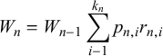 $$\begin{align*}W_n= W_{n-1}\sum_{i-1}^{k_n} p_{n,i} r_{n,i} \end{align*}$$
for $n=1,\dots ,N$
.
$n=1,\dots ,N$
.
We use W as the numeraire with which to measure the success of Jane’s martingaling. This is natural if she holds the available wealth with which she is not martingaling in W, rebalancing every day so that $p_{n,i}$
is the fraction in firm i at the beginning of day n. (In other words, she distributes across the market any capital gains, losses, or dividends she receives from holding shares of each firm.)
$p_{n,i}$
is the fraction in firm i at the beginning of day n. (In other words, she distributes across the market any capital gains, losses, or dividends she receives from holding shares of each firm.)
Let us suppose that Jane martingales by withdrawing some amount from W every day and investing it in a particular firm; say she invests $c_n$
, in units of W, in firm i during day n. The value of this investment at the end of day n, again in units of W, will be
$c_n$
, in units of W, in firm i during day n. The value of this investment at the end of day n, again in units of W, will be
 $$\begin{align*}c_n \, \frac{p_{n,i}^\prime}{p_{n,i}}, \end{align*}$$
where $p_{n,i}^\prime $
is the fraction of W due to firm i at the end of the day:
$p_{n,i}^\prime $
is the fraction of W due to firm i at the end of the day:
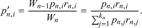 $$\begin{align*}p_{n,i}^\prime = \frac{W_{n-1}p_{n,i} r_{n,i}}{W_n} = \frac{p_{n,i} r_{n,i}}{\sum_{j=1}^{k_n}p_{n,j} r_{n,j}}. \end{align*}$$
(Because the firms in the index may change, $p_{n,i}^\prime $
may not be firm i’s share at the beginning of the next period.)
$p_{n,i}^\prime $
may not be firm i’s share at the beginning of the next period.)
She thinks she is choosing a firm that is likely to do better than the market, but we suppose that in fact she chooses randomly, with probabilities proportional the firm’s current capitalization. In other words, she chooses firm i with probability $p_{n,i}$
. The expected value of this random investment of
$p_{n,i}$
. The expected value of this random investment of $c_n$
is
$c_n$
is
 $$\begin{align*}\sum_{i=1}^{k_n} p_{n,i}\, c_n \, \frac{p_{n,i}^\prime}{p_{n,i}} = c_n. \end{align*}$$
So no matter how Jane martingales—i.e., no mater what strategy she uses to choose $c_n$
—she will have zero expected gain relative to the market:
$c_n$
—she will have zero expected gain relative to the market: $\mathbf {E}(G)=0$
and
$\mathbf {E}(G)=0$
and $\mathbf {E}(R)=\mathbf {M}$
.
$\mathbf {E}(R)=\mathbf {M}$
.
We track the capital with which Jane is martingaling just as we have done in other examples. She starts by investing one unit of W: $c_1=1$
. She puts additional money on the table as needed, never taking anything off the table until she is finished for the year. For
$c_1=1$
. She puts additional money on the table as needed, never taking anything off the table until she is finished for the year. For $n=1,\dots ,N$
, we write
$n=1,\dots ,N$
, we write $R_n$
for her cumulative return from martingaling at the end of day n: her gain divided by the total capital she has put on the table. We set
$R_n$
for her cumulative return from martingaling at the end of day n: her gain divided by the total capital she has put on the table. We set $R_0=0$
.
$R_0=0$
.
4.2.1. Mild martingaling
Suppose that on day n Jane invests in her randomly chosen firm the amount $ c_n = 1/(1+R_{n-1}). $
The initial investment is
$ c_n = 1/(1+R_{n-1}). $
The initial investment is $c_0=1$
, and later investments are less than
$c_0=1$
, and later investments are less than $1$
if Jane is doing better than the market and greater than
$1$
if Jane is doing better than the market and greater than $1$
if she is doing worse.
$1$
if she is doing worse.
Table 8 and Figure 7 show what happens on average with two different stopping rules. The first rule is to stop when $R_n\ge 0.02$
, the second is to stop when
$R_n\ge 0.02$
, the second is to stop when $R_n\ge 0.05$
. In each case, Jane plays until the end of the year if the goal is not reached. Stopping when
$R_n\ge 0.05$
. In each case, Jane plays until the end of the year if the goal is not reached. Stopping when $R_n\ge 0.02$
, Jane has a
$R_n\ge 0.02$
, Jane has a $90\%$
probability of beating the market, beating it by more than
$90\%$
probability of beating the market, beating it by more than $1\%$
on average. Stopping when
$1\%$
on average. Stopping when $R_n\ge 0.05$
, she has an
$R_n\ge 0.05$
, she has an $80\%$
probability of beating the market, beating it by
$80\%$
probability of beating the market, beating it by $2\%$
on average.
$2\%$
on average.
Table 8 Mild martingaling with randomly chosen stocks
Note: Returns relative to the S&P 500 achieved by randomly choosing a stock every day and investing $1/(1+R_{n-1})$
in it for that day. Based on a total of
$1/(1+R_{n-1})$
in it for that day. Based on a total of $4{,}200{,}000$
replications—
$4{,}200{,}000$
replications— $100{,}000$
per year for each of the 42 years from 1980 through 2021. Because
$100{,}000$
per year for each of the 42 years from 1980 through 2021. Because $\mathbf {E}(G)=0$
, the martingale index
$\mathbf {E}(G)=0$
, the martingale index $\mathbf {M}$
is equal to
$\mathbf {M}$
is equal to $\mathbf {E}(R)$
.
$\mathbf {E}(R)$
.
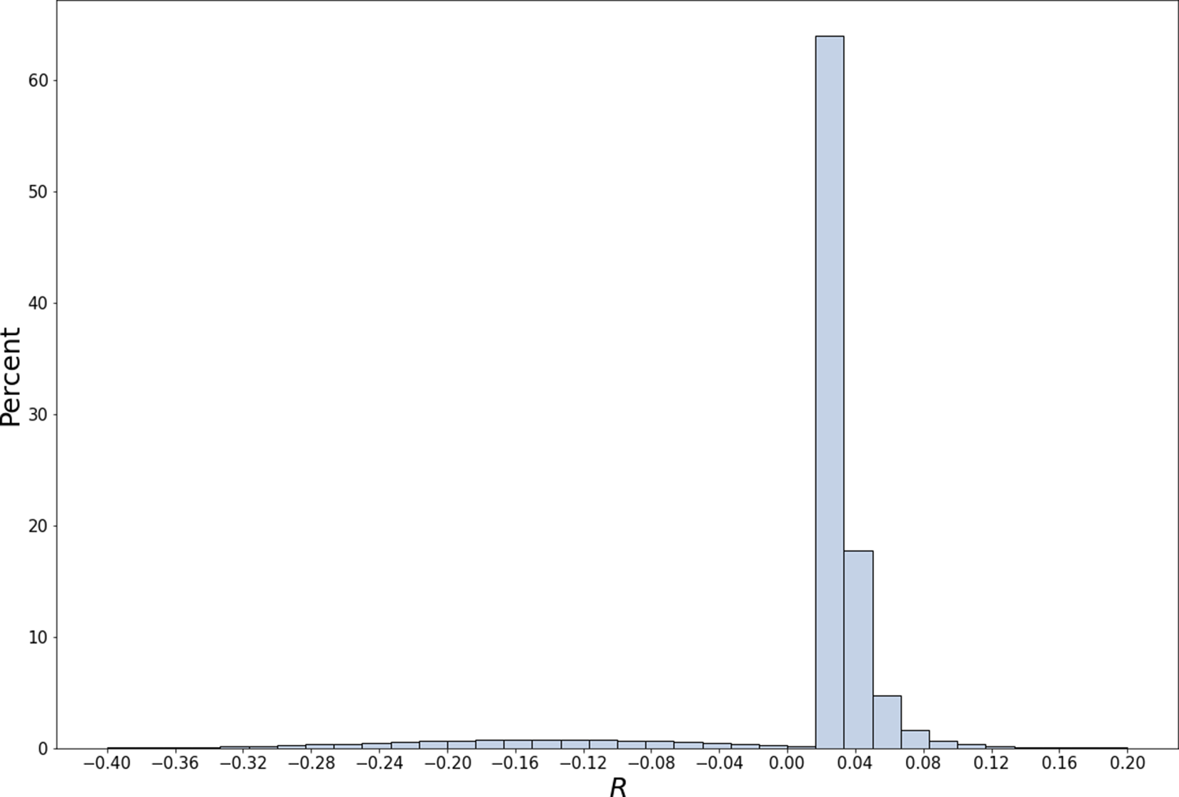
Figure 7 Distribution of returns from mild martingaling with randomly chosen stocks. Returns relative to the S&P 500 achieved by randomly choosing a stock every day and investing $1/(1+R_{n-1})$
in it for that day, stopping at
$1/(1+R_{n-1})$
in it for that day, stopping at $R_n\ge 0.02$
.
$R_n\ge 0.02$
.
Note: See also Table 8.
Returns of one or two percent are an order of magnitude smaller than we saw in trading futures on margin, where Jane had a tenfold leverage. But the probabilities in Table 8 show us that Jane is more likely than not to achieve them in just a few months—and do so several times in a row. Many people would take this success in beating the market over many months as confirmation that they have more insight into the market than the other speculators with whom they are competing.
4.2.2. More aggressive martingaling
Jane can obtain larger returns by multiplying the bet size at each step. In order to avoid excessively large or small bets, we bound the bet below by $1$
and above by
$1$
and above by $20$
:
$20$
:
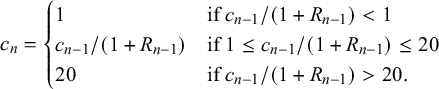 $$ \begin{align} c_n = \begin{cases} 1 & \text{if } c_{n-1}/(1+R_{n-1}) < 1\\ c_{n-1}/(1+R_{n-1}) & \text{if } 1\le c_{n-1}/(1+R_{n-1}) \le 20\\ 20 & \text{if } c_{n-1}/(1+R_{n-1})> 20. \end{cases} \end{align} $$
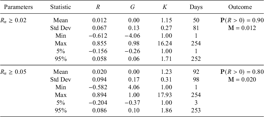
Table 9 shows simulation results for the goals $R_n\ge 0.02$
and
$R_n\ge 0.02$
and $R_n\ge 0.05$
; as before the strategies stop at the end of the year if the goal is not reached by then. The probabilities of success here rival those of the d’Alembert. The expected returns, approximately 3 and 5 percent relative to the S&P 500 are also impressive.
$R_n\ge 0.05$
; as before the strategies stop at the end of the year if the goal is not reached by then. The probabilities of success here rival those of the d’Alembert. The expected returns, approximately 3 and 5 percent relative to the S&P 500 are also impressive.
Table 9 More aggressive martingaling with randomly chosen stocks
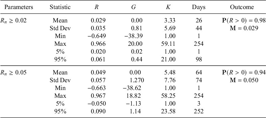
Note: Returns relative to the S&P 500 achieved by randomly choosing a stock every day and investing according to (4.1) in it for that day. Based on a total of $4{,}200{,}000$
replications—
$4{,}200{,}000$
replications— $100{,}000$
per year for each year from 1980 through 2021. Because
$100{,}000$
per year for each year from 1980 through 2021. Because $\mathbf {E}(G)=0$
, the martingale index
$\mathbf {E}(G)=0$
, the martingale index $\mathbf {M}$
is equal to
$\mathbf {M}$
is equal to $\mathbf {E}(R)$
.
$\mathbf {E}(R)$
.
5. Conclusion
The prevalence and acceptance of betting has exploded in the online age. Its negative impact on people’s lives has kept pace. Students and teachers of judgement and decision making need to find ways to educate the public about the dangers, and the martingale index can contribute to this educational mission.
The first thing everyone should learn about betting is André-Marie Ampère’s theorem of the gambler’s ruin: a gambler with finite capital who repeats the same bet persistently will be ruined with probability one, even if the house has no advantage. Jean Ville expressed this truth in a more quantitative form with his inequality of the gambler’s ruin (Ville, Reference Ville1939), now called simply Ville’s inequality: if the ratio of the house’s capital to the gambler’s capital is $\lambda $
, one of them will go bankrupt, and the probability that it will be the gambler is at least
$\lambda $
, one of them will go bankrupt, and the probability that it will be the gambler is at least $1-1/\lambda $
.
$1-1/\lambda $
.
The second thing everyone should learn about is the seductiveness of martingaling. It is an increasing danger not only in unvarnished betting, but also in finance. The ease of moving money online has made market speculation almost as accessible as betting on casino games, horse races, or sports games. The increasing acceptance of gambling has also affected the way financial trading is taught and advertised. The gambling aspect of finance was once something to be denied or obfuscated, but now it is proclaimed. Financial exchanges invent new betting markets and tout them as a social good. This makes it all the more important that the pitfalls of betting play a more prominent role in the teaching of finance at every educational level and also in research in finance and psychology.
Not even the most experienced financial practitioners are immune to martingaling. The Long-Term Capital Management fiasco showed that Nobel prize winners can fall prey to its lure. With the advent of affordable risk instruments such as the E-micros, financial martingaling becomes a danger for investors with modest means, and as we have learned, martingaling may be necessary just to maintain a position in these instruments. So researchers should think about the possibility of martingaling whenever we see steady gains attributed to maintaining a position, especially if we see skewed returns like those in Figures 6 and 7. Can the martingale index help us understand why mutual funds sell out-of-the-money options (Goetzmann et al., Reference Goetzmann, Ingersoll, Spiegel and Welch2007) or what people are doing in the carry trade (Brunnermeier et al., Reference Brunnermeier, Nagel and Pedersen2008) or in inefficient markets like the one in VIX futures (Whaley, Reference Whaley2013)?
How can we teach a wider public about the dangers of martingaling? Is recounting anecdotes about the crashes of highfliers the answer? Will such anecdotes help a sports bettor or a day trader recognize what they are doing when they start to martingale? Can anecdotes deter deliberate martingaling, or will they actually entice some to martingale? How do you tell someone who thinks they are cleverer than you that they will not know when to stop?
The martingale index, which is available to anyone who has studied a bit of statistics, goes beyond anecdote, giving arithmetic concreteness to the concept of martingaling, mathematical authority to warnings against it, and a path into more practical understanding of its temptations. It should be part of the education of anyone who studies finance, statistics, or psychology.
Data availability statement
Code and data are available at https://probabilityandfinance.com/articles/61_code_and_data.zip.
Acknowledgements
The authors acknowledge the assistance of Aniruddha Talele, Erdong Wang, and Tiangang Zhang. This paper has also benefited from comments by Ruodu Wang.
Author contributions
Conceptualization: V.D., G.S.; Data curation: V.D.; Data visualization: V.D., G.S.; Methodology: V.D., G.S.; Writing original draft: V.D., G.S. All authors approved the final submitted draft.
Competing interests
The authors declare none.
Ethical standards
The research meets all ethical guidelines, including adherence to the legal requirements of the study country.
Appendix A: Martingales and betting strategies in probability theory
How does this paper’s concept of a martingale relate to modern probability theory, where a martingale is a stochastic process whose current value is always equal to the expected value of its next value? The modern definition descends from the classical casino definition. The key step was taken by Jean Ville (Reference Ville1939), who noted that betting strategies are in a one-to-one correspondence with their resulting capital processes. These capital processes are martingales in the modern sense with respect to the betting odds.
The modern theory of martingales is treated in many textbooks, Billingsley (Reference Billingsley1995, Section 35) for example. The theory emphasizes asymptotic results, such as Doob’s martingale convergence theorem and the martingale central limit theorem. The martingales we study in this paper must stop sooner rather than later in order to do their magic, and so the asymptotic theory says nothing directly about this magic. Moreover, most of these martingales use betting rates that are disadvantageous according to the assumed or imagined probability distributions, and hence their capital processes are supermartingales rather than martingales: their current value is generally greater than the current expected value of their next value.
There is, however, a leitmotif that recurs in both modern theory and in our account of classical martingaling: a bettor has little chance of winning a great fortune if she cannot always draw on additional capital in case she has a run of bad luck. Doob’s convergence theorem, the jewel of the modern theory, implies that a martingale that is bounded below cannot grow indefinitely: with probability one it will converge to a finite value.
The modern theory of game-theoretic probability, directly inspired by Ville’s work, uses this same idea to define the probability of an event: It is the least capital a bettor needs at the outset to guarantee, without drawing on additional capital, the acquisition of unit capital if the event happens. Thus an event that enables a great multiplication of the bettor’s capital has, by definition, a very small probability (Shafer and Vovk, Reference Shafer and Vovk2019, Section 2.1). In game-theoretic statistics, this idea is used to test hypothesized probability distributions. If a bettor using the betting rates given by a probability distribution multiplies her initial capital by a large factor without drawing on additional capital, the probability distribution is discredited (Shafer, Reference Shafer2021).
We also see our leitmotif in modern finance theory’s concept of arbitrage in continuous time. The classical concept of arbitrage was simply that a trader buys at one price and sells, in a different market or under a different guise, at a higher price. There are various versions of the continuous-time concept (Shafer and Vovk, Reference Shafer and Vovk2019, pp. 401–402). One is that a trader begins with finite capital and buys and sells various securities over time without drawing on any additional capital in such a way that with probability one she does not lose money and with positive probability she makes money. Levental and Skorohod (Reference Levental and Skorohod1995) give conditions on the probabilities for the securities’ price processes that are necessary and sufficient to prevent arbitrage in this sense. They call strategies for trading that do not draw on additional capital tame portfolios.
The classical concept uses the more realistic setting of discrete time. But the fundamental point is the same: it is the prohibition on indefinitely drawing on additional capital that keeps the martingaler from making money for sure. As a reviewer has suggested, we might borrow Leventhal and Skorohod’s terminology, calling martingales that obey this prohibition tame and calling our martingale index a measure of the effect of a martingale’s departure from tameness.
Appendix B: The logarithmic return
We have used the martingale index to take account of an average simple return being misleadingly optimistic under martingaling. We already know that simple returns are misleadingly optimistic when gains are reinvested, and in this case we use logarithmic returns instead. Can logarithmic returns also be helpful for understanding martingaling? No.
To spell this out, let us first review how the logarithmic return differs from the simple return. The logarithmic return is given by
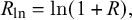 $$\begin{align*}R_{\text{ln}} = \ln (1+R), \end{align*}$$
where R is the simple return and ln is the natural logarithm. Logarithmic and simple returns differ substantially only when they are relatively large. When $R=0.01$
,
$R=0.01$
, $R_{\text {ln}}\approx 0.00995$
, and when
$R_{\text {ln}}\approx 0.00995$
, and when $R=0.1$
,
$R=0.1$
, $R_{\text {ln}}\approx 0.095$
. But when
$R_{\text {ln}}\approx 0.095$
. But when $R=1$
,
$R=1$
, $R_{\text {ln}}\approx 0.069$
, and when
$R_{\text {ln}}\approx 0.069$
, and when $R=10$
,
$R=10$
, $R_{\text {ln}}\approx 2.3$
.
$R_{\text {ln}}\approx 2.3$
.
Now let us review why logarithmic returns are useful when you are not martingaling. Suppose you invest $K_0$
and keep it invested over N time periods, neither withdrawing nor adding capital along the way. For
$K_0$
and keep it invested over N time periods, neither withdrawing nor adding capital along the way. For $n=1,\dots ,N$
, let
$n=1,\dots ,N$
, let $G_n$
be your gain each for the nth period,
$G_n$
be your gain each for the nth period, $K_n$
your capital at the end of the nth period, and
$K_n$
your capital at the end of the nth period, and $R_n$
your simple return for the nth period. Then
$R_n$
your simple return for the nth period. Then
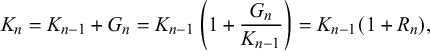 $$ \begin{align*} K_n = K_{n-1} + G_n = K_{n-1}\left(1 + \frac{G_n}{K_{n-1}}\right) = K_{n-1}(1 + R_n), \end{align*} $$
again for $n=1,\dots ,N$
. It follows that
$n=1,\dots ,N$
. It follows that $K_N=K_0(1+R_1)\cdots (1+R_N)$
. Thus the overall simple return R satisfies
$K_N=K_0(1+R_1)\cdots (1+R_N)$
. Thus the overall simple return R satisfies
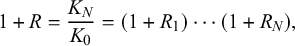 $$\begin{align*}1+R = \frac{K_N}{K_0}=(1+R_1)\cdots(1+R_N), \end{align*}$$
and the logarithmic returns add:
 $$ \begin{align} \ln(1+R) =\ln(1+R_1)+\dots+\ln(1+R_N). \end{align} $$
Because the logarithmic returns add, you can use them to monitor how your investment changes as time proceeds.
But (5.1) is not valid when an investor is martingaling. To make it valid, we would need to recalculate all the $R_n$
to take the martingaling into account. From our all-knowing perch, we could do this for the martingaler’s return
$R_n$
to take the martingaling into account. From our all-knowing perch, we could do this for the martingaler’s return $G/K$
or for the strategy’s return
$G/K$
or for the strategy’s return $G/\textbf {K}$
, but neither exercise is directly relevant to the deceptiveness of martingaling. The martingaler herself could not even do these calculation as time proceeds, because she does not know K until she stops, and she may never know
$G/\textbf {K}$
, but neither exercise is directly relevant to the deceptiveness of martingaling. The martingaler herself could not even do these calculation as time proceeds, because she does not know K until she stops, and she may never know $\textbf {K}$
.
$\textbf {K}$
.


 Open access