


1. Introduction
In the early 1990s, central banks of New Zealand, Canada, and the United Kingdom officially adopted an inflation-targeting regime, which was later followed by numerous other countries. Since then, determining the optimal inflation target has become a central focus in monetary policy research.Footnote 1 The existing literature presents a wide range of estimates for the optimal inflation target. Early studies proposed negative optimal inflation rates mainly based on Friedman rule (Cooley and Hansen, Reference Cooley and Hansen1989; Chari et al. Reference Chari, Christiano and Kehoe1996; Schmitt-Grohé and Uribe, Reference Schmitt-Grohé and Uribe2004), whereas more recent papers suggest positive inflation rates (Kim and Ruge-Murcia, Reference Kim and Ruge-Murcia2011; Blanco, Reference Blanco2021; Adam and Weber, Reference Adam and Weber2023), with some advocating for rates as high as 5% (Fagan and Messina, Reference Fagan and Messina2009).
An important motivation for targeting a high inflation rate is the friction in the labor market called downward nominal wage rigidity (DNWR)–the inability of firms to reduce nominal wages.Footnote 2 A higher inflation rate provides firms with the flexibility to reduce wages in real terms while keeping nominal wages constant. So, higher inflation relaxes this constraint but at the same time increases the welfare cost associated with price dispersion.Footnote 3 Since DNWR is a friction at the worker level and affects the cross-section of individual wage changes, a representative agent economy cannot fully capture its effects. A constraint on aggregate wages fails to account for micro-level frictions, leading to an underestimation of the impact of this labor market friction and, consequently, the benefits of higher inflation. For DNWR to play a significant role, it is crucial to fully account for worker heterogeneity (Daly and Hobijn, Reference Daly and Hobijn2014). Accordingly, this study uses a heterogeneous-agent New Keynesian model to quantify the trade-offs and identify the welfare-maximizing steady-state inflation rate. Second, the quantitative importance of DNWR depends heavily on how the nominal friction is specified and calibrated. To address this, different wage-setting models have been considered to capture the DNWR constraint, and key parameters are calibrated based on recent empirical evidence on DNWR.Footnote 4 The findings reveal that DNWR significantly influences the economy, with the optimal steady-state inflation rate estimated to be as high as 9%, yielding welfare gains of approximately 3.60%. Although the optimal inflation target is sensitive to parameter choices, it consistently exceeds 3% across a broad range of calibrations.
Data on annual wage changes reveal that nominal wages exhibit downward rigidity, as nominal wage cuts are rare and a substantial proportion of employees experience no change in their nominal wage. This phenomenon, known as downward nominal wage rigidity, generates a trade-off between inflation and unemployment at low inflation rates. Specifically, some firms may need to reduce real wages due to the stochastic nature of productivity, but in a low inflation regime, this necessitates nominal wage cuts, which are not commonly practiced by convention. Thus, if the inflation rate is low and nominal wage cuts are not feasible, firms resort to layoffs instead. As a result, positive shocks result in wage increases, while negative shocks lead to increased unemployment. To put it differently, the long-run Phillips curve approaches verticality at high inflation and flattens out at low inflation, indicating a progressive increase in the output cost of reducing inflation (Daly and Hobijn, Reference Daly and Hobijn2014).
According to Tobin (Reference Tobin1972), when DNWR is pronounced, positive inflation acts as a lubricant (“greases the wheels”) for the economy by promoting wage flexibility. A positive inflation rate allows for greater downward real wage adjustments in response to shocks, as it provides more leeway for real wage cuts while keeping nominal wages constant. Hence, a higher inflation rate may be desirable to accommodate a wider range of real wage reductions.
Both survey data (Akerlof et al. Reference Akerlof, Dickens, Perry, Gordon and Mankiw1996; Daly and Hobijn, Reference Daly and Hobijn2014; Fallick et al. Reference Fallick, Lettau and Wascher2016) and administrative data (Kurmann and Mcentarfer, Reference Kurmann and Mcentarfer2019; Jardim et al. Reference Jardim, Solon and Vigdor2019; Grigsby et al. Reference Grigsby, Hurst and Yildirmaz2021) indicate that DNWR is empirically valid in the U.S. This phenomenon has also been observed in other countries as shown by Dickens et al. (Reference Dickens, Goette, Groshen, Holden, Messina, Schweitzer, Turunen and Ward2007), who document the empirical wage change distribution based on cross-country datasets. In the U.S., the rate of no wage change–defined as the proportion of employees experiencing no nominal wage adjustment within a year–has ranged from 5% to 25% since 1980 and can reach up to 35% when considering only base wage changes, as documented by Grigsby et al. (Reference Grigsby, Hurst and Yildirmaz2021).Footnote 5 Furthermore, the correlation between the inflation rate and the rate of no wage change from 1980 to 2020 is −0.65 (see Figure-C2), supporting Tobin’s original idea that higher inflation should result in fewer nominal wage freezes.
While nominal wage freezes are common in the data, a non-negligible proportion of nominal wage cuts is also observed. According to Grigsby et al. (Reference Grigsby, Hurst and Yildirmaz2021), the rate of wage cuts is 15.7% when bonuses are included and 2.5% when only base wages are considered.Footnote 6 Given the high level of wage freezes and missing cuts in the empirical distribution, a model with a DNWR constraint imposed on aggregate wages within a representative agent framework–restricting aggregate wages from falling below a certain threshold–may fail to accurately capture empirical findings. In reality, DNWR is binding for a subset of households in each period. To effectively analyze the welfare costs of DNWR, a model must replicate the empirical wage change distribution, which necessitates the use of a heterogeneous-agent framework. That is, to address DNWR more accurately, one needs to consider the heterogeneity in productivity at the household level. Firms seek to decrease the real wages of workers who receive negative idiosyncratic productivity shocks in a period. In a low inflation environment, real wage cuts are limited, leading to significant welfare costs due to the inability to adjust wages optimally. However, this is offset to some extent by the lower welfare cost of price dispersion in a low-inflation environment.
I incorporate the DNWR constraint into an otherwise standard New Keynesian model, and then analyze the welfare costs at various steady-state inflation rates in order to determine the optimal inflation rate in this standard model to make the results comparable to the previous literature. It examines the trade-off between the “grease” effect of inflation, which alleviates the DNWR constraint, and the “sand” effect of inflation, which captures the costs of price dispersion and inefficient price setting. In a low-inflation environment, the grease effect dominates, whereas at higher inflation rates, the sand effect becomes more pronounced. In other words, while a higher inflation target reduces the welfare cost associated with DNWR, it simultaneously increases the welfare cost of price dispersion. This trade-off is central to the welfare analysis and enables the identification of the economy’s optimal inflation rate. Here, the model abstracts from other potential costs of higher inflation, such as increased macroeconomic volatility, higher markups, and dispersed inflation expectations (Ascari and Sbordone, Reference Ascari and Sbordone2014), and instead focuses solely on the trade-off between DNWR and the distortion in relative prices caused by inflation, which represents the standard cost of inflation in sticky price models.
I match the wage change distribution using a simple heterogeneous-agent model with an asymmetrically staggered wage-setting mechanism, as proposed by Daly and Hobijn (Reference Daly and Hobijn2014). After calibrating the model, I solve it for different steady-state inflation rates and conduct a welfare comparison. According to the steady-state welfare analysis, the optimal steady-state inflation rate is approximately 7%, rather than the current target of 2%, and could be as high as 9% when considering only changes in base wages. Even under extreme levels of price stickiness and the resulting cost of inflation, the model suggests an optimal rate above 3%. In a standard New Keynesian framework, with only minor modifications to the wage-setting mechanism to imitate the DNWR constraint, I find that the optimal inflation rate is considerably higher than the 2% benchmark set by the Federal Reserve or the slightly positive rates typically regarded as ”normal.” This finding is quite robust to changes in the nearly all parameters in a standard model. By accounting for the nonlinearity introduced by DNWR in the labor market, the result inferred from a very standard model is significantly different from previous literature.
The paper is structured as follows: In Section 2, I review the relevant literature and outline my contribution. Section 3 presents the model, a heterogeneous-agent New Keynesian framework incorporating the DNWR constraint at the household level. Section 4 presents the steady-state results and Section 5 includes a sensitivity analysis of the steady-state results. Section 6 presents the results obtained from the model with asymmetric menu cost wage setting as an alternative to the benchmark model with asymmetric Calvo-type wage setting. Finally, Section 7 concludes the paper.
2. Related literature
Downward nominal wage rigidity has become an important research topic that can leverage recent increases in computational capabilities. Elsby (Reference Elsby2009) analyzes the distribution of wage changes using a partial equilibrium model that incorporates DNWR and evaluate its implications for aggregate wage growth. Their main finding is that while DNWR prevents wage cuts, it also suppresses wage increases, leading to the conclusion that the macroeconomic effects of DNWR are limited.
Kim and Ruge-Murcia (Reference Kim and Ruge-Murcia2009) and Kim and Ruge-Murcia (Reference Kim and Ruge-Murcia2011) introduce an asymmetric cost to wage adjustments and analyze the effect of DNWR on the optimal level of “grease” inflation, in a representative agent model. They conclude that the optimal inflation target should be near 1 percent. Benigno and Ricci (Reference Benigno and Ricci2011), on the other hand, incorporate a DNWR constraint into individual wage-setting problems in a heterogeneous-sector model, accounting for both idiosyncratic and aggregate shocks. They explore the implications of DNWR for the shape of the Phillips curve and conclude that positive inflation can facilitate both intratemporal and intertemporal relative price adjustments, although they do not provide an estimate for the optimal inflation rate.
Fagan and Messina (Reference Fagan and Messina2009) utilize a modified menu cost model for wage setting and conduct a welfare analysis, determining that the optimal inflation target under DNWR is 2 percent but can vary up to 5 percent based on estimates for the probability of menu costs within the model.Footnote 7 If half of households are exempt from menu cost constraints annually, the optimal rate is estimated at 2 percent, increasing to 5 percent if the binding frequency of menu costs rises to 80 percent. Daly and Hobijn (Reference Daly and Hobijn2014) employ a discrete-time model to analyze the mechanism behind the flattening of the Phillips curve by incorporating the DNWR constraint, similar to Benigno and Ricci (Reference Benigno and Ricci2011), and they solve for transition dynamics in response to demand and supply shocks to analyze the bending of the Phillips curve. They examine the relationship between the unemployment rate and the degree of downward nominal wage rigidity. Schmitt-Grohe and Uribe (Reference Schmitt-Grohe and Uribe2016) introduce a DNWR constraint for the aggregate wage in a standard representative agent model and analyze the impact of currency peg in this setting. Amano and Gnocchi (Reference Amano and Gnocchi2023) and Billi and Galí (Reference Billi and Galí2020) document that wage rigidity reduces the severity of demand-driven recessions, particularly during zero lower bound periods, in a representative agent setting. In this context, the aggregate DNWR constraint is binding in a demand-driven recession, distorting the labor market but making marginal costs rigid, thereby decreasing the volatility of inflation and the zero lower bound binding frequency. Consequently, wage flexibility might decrease welfare in such recessions.Footnote 8 Jo (Reference Jo2021) analyzes different wage-setting schemes in the literature and shows that a model with a downward nominal wage rigidity constraint is the most consistent with empirical findings regarding the wage change distributions.
Mineyama (Reference Mineyama2022) employs a wage-setting framework with asymmetric adjustment costs, similar to Fagan and Messina (Reference Fagan and Messina2009), to match the empirical distribution of wage changes and estimates an optimal inflation target between 1.4 percent and 2.6 percent. The model’s parameterization plays a significant role in producing a relatively low welfare cost associated with the downward nominal wage rigidity constraint. Additionally, the assumption of wage flexibility for job switchers further reduces the welfare cost; however, Hazell and Taska (Reference Hazell and Taska2020) document that wages for new hires are also downwardly rigid. The paper discusses the differences between the model presented here and Mineyama (Reference Mineyama2022) in a dedicated section, comparing the results accordingly.
The present model adopts a simpler wage-setting mechanism that deviates slightly from the standard New Keynesian model to match the annual wage change distribution, thereby enhancing its comparability to prior literature. A simplified DNWR constraint, widely used in recent studies, is employed to capture labor market dynamics and explain the flattening of the Phillips Curve in a straightforward manner. The primary contribution of this study lies in implementing the DNWR constraint, as utilized in recent papers (Guerrieri et al. (Reference Guerrieri, Lorenzoni, Straub and Werning2021, Reference Guerrieri, Lorenzoni, Straub and Werning2022); Schmitt-Grohe and Uribe (Reference Schmitt-Grohe and Uribe2016); Shen and Yang (Reference Shen and Yang2018); Dupraz et al. (Reference Dupraz, Nakamura and Steinsson2025); Jo and Zubairy (Reference Jo and Zubairy2025); Rouillard (Reference Rouillard2023)) and demonstrating its welfare implications. While this approach has become standard in macroeconomic modeling, its welfare implications have not been thoroughly explored. This study highlights that the DNWR constraint, when calibrated to match the empirical wage change distribution, generates substantial welfare costs and should be incorporated cautiously into standard models.Footnote 9 In summary, this study employs a widely adopted version of the DNWR constraint and conducts a steady-state welfare analysis across various trend inflation rates to evaluate the welfare costs associated with DNWR.Footnote 10
I match the annual wage change distribution by using the most recent empirical data based on the estimates of Grigsby et al. (Reference Grigsby, Hurst and Yildirmaz2021), derived from administrative data, and the San Francisco Fed’s wage rigidity estimates, which are based on the Current Population Survey (CPS) data.Footnote 11 The empirical match is crucial for the welfare analysis because the significance of the DNWR channel depends on the wage freeze rate in the annual wage change distribution.Footnote 12 The model assumes no aggregate uncertainty and focuses on this cross-sectional heterogeneity. To the best of my knowledge, Coibion et al. (Reference Coibion, Gorodnichenko and Wieland2012) - which analyzes optimal steady-state inflation using a standard representative-agent New Keynesian model without heterogeneity - is the closest paper, in terms of the main research idea. They find that the optimal inflation may range from 1% to 3% depending on assumptions related to price stickiness, DNWR, zero lower bound, and uncertainty. To facilitate a meaningful comparison with their findings, I calibrate my model by closely following their approach. This allows me to document how the DNWR constraint influences the optimal inflation rate in a heterogeneous-agent model within a standard New Keynesian framework. The main finding is that the optimal inflation rate is approximately 7%, with its level shaped to some extent by the parameterization and the modeling approach. However, the conclusion of a higher optimal inflation rate–significantly above the conventional 2% target–remains robust across alternative calibrations and wage-setting mechanisms. Importantly, this study quantifies the welfare impact of the DNWR constraint and estimates the optimal inflation target while also accounting for the “sand” effect of price dispersion in the economy.
3. Model
I employ a New Keynesian model, which includes a standard Calvo pricing friction but an asymmetric wage setting friction, following Daly and Hobijn (Reference Daly and Hobijn2014) and Jo (Reference Jo2021). The households are heterogeneous in their productivity levels. Basically, I introduce a downward wage rigidity setting into an otherwise standard New Keynesian model without capital accumulation.
3.1 Households
In this economy, there is a continuum of households, indexed by i on the unit interval and they supply differentiated labor input to the labor packer. Households differ in their productivity due to idiosyncratic productivity shocks they receive each period. The labor packer combines labor into aggregate labor with the following Dixit-Stiglitz technology:
 \begin{equation*} L_{t}=\left (\int _{0}^{1} (q_t(i) l_{t}(i))^{\frac {\epsilon _{w}-1}{\epsilon _{w}}} d i\right)^{\frac {\epsilon _{w}}{\epsilon _ w-1}}, \end{equation*}
where idiosyncratic shock $q_t(i)$
follows AR(1) process:
$q_t(i)$
follows AR(1) process:
 \begin{equation*} \ln \left (q_{t+1}(i)\right)=\rho _{q} \ln \left (q_{t}(i)\right)+\epsilon _{t+1}(i), \quad \epsilon _{t+1}(i) \sim \mathbb{N}\left (0, \sigma _{q}^{2}\right). \end{equation*}
The idiosyncratic productivity process is assumed to be persistent, unlike Daly and Hobijn (Reference Daly and Hobijn2014), and the persistency is calibrated based on Guvenen (Reference Guvenen2009) to make it as standard as possible.Footnote 13
The maximization problem of the competitive labor packer is
 \begin{equation*} \max _{l_t(i)} W_t L_t - \int _{0}^{1} W_t(i) l_t(i). \end{equation*}
The first-order condition of the cost minimization problem of labor packer implies
 \begin{equation*} W_t \frac {\epsilon _w}{\epsilon _w-1} \left (\int _{0}^{1} (q_t(i) l_{t}(i))^{\frac {\epsilon _{w}-1}{\epsilon _{w}}} d i\right)^{\frac {1}{\epsilon _ w-1}} q_t(i)^\frac {\epsilon _w-1}{\epsilon _w} l_t(i)^\frac {-1}{\epsilon _w} \frac {\epsilon _w-1}{\epsilon _w} = W_t(i). \end{equation*}
Then, I can get the labor demand as
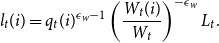 \begin{equation*} l_{t}(i)=q_{t}(i)^{\epsilon _w-1}\left (\frac {W_{t}(i)}{W_{t}}\right)^{-\epsilon _w} L_{t}. \end{equation*}
The relative demand for labor of type i is a function of its relative wage, productivity, and the elasticity $\epsilon _{w}$
. Using the demand, I can find aggregate wage as
$\epsilon _{w}$
. Using the demand, I can find aggregate wage as
 \begin{equation*} W_{t}=\left [\int _{0}^{1}\left (\frac {W_{t}(i)}{q_{t}(i)}\right)^{1-\epsilon _{w}} d i \right]^{\frac {1}{1-\epsilon _{w}}}, \end{equation*}
which can be written in terms of real wage as well.
Households have CRRA utility and their preferences are additively separable in consumption and labor. They choose consumption, saving as nominal stock of bonds, nominal wage, and labor supply to maximize the expected lifetime utility. The following is the maximization problem of households
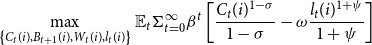 \begin{equation*}\max _{\left \{C_{t}(i), B_{t+1}(i), W_{t}(i), l_{t}(i)\right \}} \mathbb{E}_{t} \Sigma _{t=0}^{\infty } \beta ^{t}\left [\frac {C_{t}(i)^{1-\sigma }}{1-\sigma }-\omega \frac {l_{t}(i)^{1+\psi }}{1+\psi } \right] \end{equation*}
subject to
 \begin{gather*} P_{t} C_{t}(i)+ \mathbb{E}_t Q_{t+1} B_{t+1}(i) \leq B_{t}(i)+W_{t}(i) l_{t}(i)+\Pi _{t}, \\ l_{t}^{d}(i)=q_{t}(i)^{\epsilon _w-1}\left (\frac {W_{t}(i)}{W_{t}}\right)^{-\epsilon _w} L_{t}, \\ \text{and }\textbf {DNWR}\text{ constraint,} \end{gather*}
where price of consumption good $P_t$
, unique stochastic discount factor
$P_t$
, unique stochastic discount factor $Q_{t+1}$
and aggregate labor supply
$Q_{t+1}$
and aggregate labor supply $L_t$
are taken as given by households.
$L_t$
are taken as given by households. $\Pi _t$
is profit distributed lump sum to households. Here, the downward nominal wage rigidity (DNWR) constraint is defined as
$\Pi _t$
is profit distributed lump sum to households. Here, the downward nominal wage rigidity (DNWR) constraint is defined as
 \begin{equation*} \text{if } w_t^*(i) \geq \frac {w_{t-1}(i)}{\pi _t A_t} \quad \begin{cases} w_t(i)=w_t^*(i), \end{cases} \end{equation*}
 \begin{equation*} \text{if } w_t^*(i) \lt \frac {w_{t-1}(i)}{\pi _t A_t} \quad \begin{cases} w_t(i)=\frac {w_{t-1}(i)}{\pi _t A_t} \quad \text{with the prob } \mu ^{DNWR} \\ w_t(i)=w_t^*(i) \quad \text{with the prob } (1-\mu ^{DNWR}) \end{cases} \end{equation*}
where $w_t^*$
is the optimal real wage of households if the constraint does not bind and solution to the maximization problem presented below. Here, households adjust their nominal wages upwards without restriction, but they are only able to decrease their nominal wages with a probability of
$w_t^*$
is the optimal real wage of households if the constraint does not bind and solution to the maximization problem presented below. Here, households adjust their nominal wages upwards without restriction, but they are only able to decrease their nominal wages with a probability of $1-\mu ^{DNWR}$
. Otherwise, if they are unable to decrease their nominal wages, they must keep them constant. This does not eliminate real wage cuts completely because if inflation is positive, keeping the nominal wage constant is simply a real wage cut. There is also aggregate productivity growth factor
$1-\mu ^{DNWR}$
. Otherwise, if they are unable to decrease their nominal wages, they must keep them constant. This does not eliminate real wage cuts completely because if inflation is positive, keeping the nominal wage constant is simply a real wage cut. There is also aggregate productivity growth factor $A_t$
, which provides additional scope for real wage reductions.Footnote
14
$A_t$
, which provides additional scope for real wage reductions.Footnote
14
The DNWR constraint simply implies an asymmetric Calvo wage setting scheme, where households have flexibility in increasing their wages but are restricted from decreasing them with some probability. Due to idiosyncratic productivity shocks, some households each period may wish to decrease their wages, but the DNWR constraint may prevent them from doing so, causing a spike in the wage freeze rate in the wage change distribution. Depending on the value of $\mu ^{DNWR}$
, some households may be able to decrease their wages, which constitutes wage cuts in the wage change distribution. This friction leads to differences in wages across households and, therefore, differences in the labor hours supplied by each household.
$\mu ^{DNWR}$
, some households may be able to decrease their wages, which constitutes wage cuts in the wage change distribution. This friction leads to differences in wages across households and, therefore, differences in the labor hours supplied by each household.
In this framework, I assume that households have access to complete state-contingent assets, allowing for complete consumption insurance and uniformity of consumption across households (Benigno and Ricci, Reference Benigno and Ricci2011), as a result of their separable utility functions.
 \begin{equation*} C_t(i) = C_t \end{equation*}
Market completeness ensures that there is a unique stochastic discount factor that prices any asset. The first-order condition for households with respect to nominal bond holdings
 \begin{equation*} \begin{array}{c} \mathbb{E}_{t}\left [ Q_{t+1} i_t \right]=1 \end{array} \end{equation*}
where the nominal discount factor is $Q_{t+1} = \beta \frac {u^{\prime}(C_{t+1})}{u^{\prime}(C_t)} \frac {P_t}{P_{t+1}}$
and
$Q_{t+1} = \beta \frac {u^{\prime}(C_{t+1})}{u^{\prime}(C_t)} \frac {P_t}{P_{t+1}}$
and $i_t$
denotes the gross nominal interest rate. The Euler equation can be derived from the first-order conditions for consumption and nominal bond holdings.
$i_t$
denotes the gross nominal interest rate. The Euler equation can be derived from the first-order conditions for consumption and nominal bond holdings.
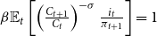 \begin{equation*} \begin{array}{c} \beta \mathbb{E}_{t}\left [\left (\frac {C_{t+1}}{C_{t}}\right)^{-\sigma } \frac {i_{t}}{\pi _{t+1}}\right]=1 \end{array} \end{equation*}
Since there is no capital in this economy, all production is consumed. Output is equal to consumption and I can rewrite the Euler equation as
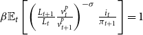 \begin{equation*} \begin{array}{c} \beta \mathbb{E}_{t}\left [\left (\frac {L_{t+1}}{L_{t}}\frac {v_{t}^p}{v_{t+1}^p}\right)^{-\sigma } \frac {i_{t}}{\pi _{t+1}}\right]=1 \end{array} \end{equation*}
where $\pi _t$
is inflation rate,
$\pi _t$
is inflation rate, $v_t^p$
is price dispersion, and
$v_t^p$
is price dispersion, and $i_t$
is nominal interest rate.
$i_t$
is nominal interest rate.
Due to heterogeneity in productivity (as a result of uninsurable idiosyncratic productivity shocks), the labor supply differs across households, and leisure is not fully insured. Two Bellman equations characterize the dynamic planning problem of a household. Given the aggregates $\Gamma _t \equiv \{ L_t,\pi _t,v_t^p \}$
, the value function for constrained households, who cannot nominally decrease their wages, can be written as
$\Gamma _t \equiv \{ L_t,\pi _t,v_t^p \}$
, the value function for constrained households, who cannot nominally decrease their wages, can be written as
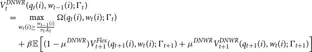 \begin{align*} & V^{DNWR}_t(q_t(i),w_{t-1}(i);\;\Gamma _t) \\ &\quad = \max _{w_t(i) \geq \frac {w_{t-1}(i)}{\pi _t A_t} } \Omega (q_t(i),w_t(i);\;\Gamma _t)\\ &\qquad + \beta \mathbb{E} \left [ (1-\mu ^{DNWR}) V^{Flex}_{t+1} (q_{t+1}(i),w_{t}(i);\;\Gamma _{t+1}) + \mu ^{DNWR} V^{DNWR}_{t+1} (q_{t+1}(i),w_{t}(i);\;\Gamma _{t+1})\right] \end{align*}
And the value function for households that can change their wages flexibly is
 \begin{align*} &V^{Flex}_t(q_t(i),w_{t-1}(i);\;\Gamma _t)\\ &\quad = \max _{w_t(i)} \quad \Omega (q_t(i),w_t(i);\;\Gamma _t)\\ & \qquad + \beta \mathbb{E} \left [ (1-\mu ^{DNWR}) V^{Flex}_{t+1} (q_{t+1}(i),w_{t}(i);\;\Gamma _{t+1}) + \mu ^{DNWR} V^{DNWR}_{t+1} (q_{t+1}(i),w_{t}(i);\;\Gamma _{t+1})\right] \end{align*}
where
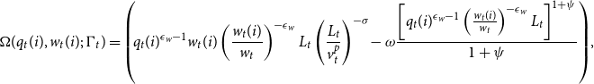 \begin{equation*} \Omega (q_t(i),w_t(i);\;\Gamma _t)= \left (\! q_{t}(i)^{\epsilon _w-1}w_{t}(i)\left (\frac {w_{t}(i)}{w_{t}}\right)^{-\epsilon _w} L_{t} \left (\frac {L_t}{v_t^p}\right)^{-\sigma }\!-\omega \frac {\left [q_{t}(i)^{\epsilon _w-1}\left (\frac {w_{t}(i)}{w_{t}}\right)^{-\epsilon _w} L_{t}\right]^{1+\psi }}{1+\psi } \right)\!, \end{equation*}
and $w_t$
is real detrended aggregate wage,
$w_t$
is real detrended aggregate wage, $L_t$
is aggregate labor supply,
$L_t$
is aggregate labor supply, $v_t^p$
is price dispersion, and
$v_t^p$
is price dispersion, and $A_t$
is trend productivity growth, which is assumed to be constant.Footnote
15
$A_t$
is trend productivity growth, which is assumed to be constant.Footnote
15
For constrained households, wages in the current period cannot go below nominal wages set in the previous period. Households, who are allowed to change, are free to set their nominal wages flexibly, but they know the DNWR constraint might bind in the future.Footnote
16
Daly and Hobijn (Reference Daly and Hobijn2014) analytically prove that the ones who are subject to DNWR constraint keep their nominal wages constant (a real wage cut), which creates the wage freeze rate in the wage change distribution. The parameter $\mu ^{DNWR}$
and the idiosyncratic productivity process affect the wage freeze and cut rates, and the model can be calibrated using this degree of freedom.
$\mu ^{DNWR}$
and the idiosyncratic productivity process affect the wage freeze and cut rates, and the model can be calibrated using this degree of freedom.
3.2 Firms
There are two types of firms: final good and intermediate good firms. The final good $Y_t$
is produced as a combination of a continuum of intermediate goods
$Y_t$
is produced as a combination of a continuum of intermediate goods $Y_{t}(j)$
with j
$Y_{t}(j)$
with j $\in$
(0,1).
$\in$
(0,1).
 \begin{equation*} Y_{t} = \bigg ( \int _{0}^{1} Y_{t}(j)^\frac {\epsilon _p-1}{\epsilon _p} \bigg)^\frac {\epsilon _p}{\epsilon _p-1}, \end{equation*}
where $\epsilon _p$
is greater than 1. The profit maximization problem of the final goods firm is
$\epsilon _p$
is greater than 1. The profit maximization problem of the final goods firm is
 \begin{align*} \max _{Y_{t}(j)} \quad P_{t}\left (\int _{0}^{1} Y_{t}(j)^{\frac {\epsilon _p-1}{\epsilon _p}}\right)^{\frac {\epsilon _p}{\epsilon _p-1}}-\int _{0}^{1} P_{t}(j) Y_{t}(j) d j. \end{align*}
As a result, I can write the output of firm j as
 \begin{equation} Y_{t}(j)=\left (\frac {P_{t}(j)}{P_{t}}\right)^{-\epsilon _p} Y_{t}. \end{equation}
Then, it is straightforward to derive the price as
 \begin{align*} P_{t} = \bigg ( \int _{0}^{1} P_{t}(j)^{1-\epsilon _p} \bigg)^\frac {1}{1-\epsilon _p}. \end{align*}
Monopolist intermediate goods producer $j$
produces according to a constant return to scale technology.
$j$
produces according to a constant return to scale technology.
 \begin{equation} Y_t(j) = A_t L_t(j). \end{equation}
There is a single sector in this economy and firms are identical (representative firm). Intermediate goods firms rent labor in a perfectly competitive market. Each period, they try to minimize their cost by solving the following problem
 \begin{align*} \min _{L_{t}(j)} W_{t} L_{t}(j) \quad \text{subject to (2)} \end{align*}
Then, the first-order condition is
 \begin{align*} MC_{t}(j)=\frac {W_{t}}{A_{t}} \equiv M C_{t}. \end{align*}
where $MC_t$
is nominal marginal cost and identical across intermediate goods firms due to facing common wage in the market. Then, I can define real marginal cost as
$MC_t$
is nominal marginal cost and identical across intermediate goods firms due to facing common wage in the market. Then, I can define real marginal cost as $mc_t = \frac {MC_t}{P_t}$
.
$mc_t = \frac {MC_t}{P_t}$
.
Firms set prices through the Calvo mechanism. Every period, with some probability (1- $\mu _p$
), firms are able to reset their prices optimally. In this setting, the dynamic problem of a firm is the following:
$\mu _p$
), firms are able to reset their prices optimally. In this setting, the dynamic problem of a firm is the following:
 \begin{align*} \max _{P_{t}(j)} \quad \mathbb{E}_{t} \sum _{s=0}^{\infty }\left (\beta \mu _{p}\right)^{s} \left (\frac {C_{t+s}}{C_t}\right)^{-\sigma }\left (\frac {P_{t}(j)}{P_{t+s}}\left (\frac {P_{t}(j)}{P_{t+s}}\right)^{-\epsilon _{p}} Y_{t+s}-m c_{t+s}\left (\frac {P_{t}(j)}{P_{t+s}}\right)^{-\epsilon _{p}} Y_{t+s}\right). \end{align*}
Firms solve the profit maximization problem and choose the optimal price. After getting FOC, it can be simplified into
 \begin{align*} P_t^* = P_{t}^*(j)=\frac {\epsilon _p}{\epsilon _p-1} \frac {\mathbb{E}_{t} \sum _{s=0}^{\infty }(\beta \mu _p)^{s} C_{t+s}^{-\sigma } m c_{t+s} P_{t+s}^{\epsilon _p} Y_{t+s}}{\mathbb{E}_{t} \sum _{s=0}^{\infty }(\beta \mu _p)^{s} C_{t+s}^{-\sigma } P_{t+s}^{\epsilon _p-1} Y_{t+s}}. \end{align*}
The optimal reset price $P_t^*$
is the same for every firm that is not allowed to change its prices. Finally, as shown in the literature, the price dispersion evolves according to a recursive formula
$P_t^*$
is the same for every firm that is not allowed to change its prices. Finally, as shown in the literature, the price dispersion evolves according to a recursive formula
 \begin{align*} v_t^p = \mu _p \pi _t^{\epsilon _{p}} v_{t-1}^p + (1-\mu _p) \left (\frac {P_t^*}{P_t}\right)^{-\epsilon _{p}}. \end{align*}
3.3 Monetary policy
Since both prices and wages in the economy are sticky, monetary policy has an effect on the allocation of resources. Monetary policy is given by a standard Taylor (Reference Taylor1993) rule, and the interest rate is bounded by zero.
 \begin{align*}i_{t}^*=\frac {\overline {\pi } \overline {A}}{\beta }\left (\frac {y_{t}}{\overline {y}}\right)^{\varphi _{Y}}\left (\frac {\pi _{t}}{\overline {\pi }}\right)^{\varphi _{\pi }}, \end{align*}
 \begin{align*}i_{t}= \max \{i_t^*,1\}, \end{align*}
where the central bank targets the inflation rate, $\overline {\pi }$
, but also tries to stabilize the output gap.
$\overline {\pi }$
, but also tries to stabilize the output gap. $\overline {y}$
is the steady state output and
$\overline {y}$
is the steady state output and $\overline {A}$
is the steady-state productivity growth.
$\overline {A}$
is the steady-state productivity growth.
3.4 Market clearing
Market clearing requires that the good market, asset market, and labor market clear.
 \begin{align*}Y_t=C_t, \end{align*}
 \begin{align*} B_{t} \equiv \int _{0}^{1} B_{t}(i) d i=0, \end{align*}
 \begin{align*} L_{t}=\int _{0}^{1} L_{t}(j) d j. \end{align*}
Because of fully insured consumption, the asset market trivially clears. In addition, the nominal output is equal to nominal wage payment in this economy.
 \begin{align*} P_{t} Y_{t}=P_{t} C_{t}=W_{t} L_{t}. \end{align*}
Using (1) and (2), I can write
 \begin{align*} A_{t} L_{t}(j)=\left (\frac {P_{t}(j)}{P_{t}}\right)^{-\epsilon } Y_{t}. \end{align*}
By integrating over j, I get
 \begin{align*} A_{t} \int _{0}^{1} L_{t}(j) d j= A_t L_t = Y_{t} \int _{0}^{1}\left (\frac {P_{t}(j)}{P_{t}}\right)^{-\epsilon } d j. \end{align*}
So, the aggregation gives the output at time t
 \begin{equation} Y_t = \frac {A_{t} \left (\int _{0}^{1} (q_t(i) l_{t}(i))^{\frac {\epsilon _{w}-1}{\epsilon _{w}}} d i\right)^{\frac {\epsilon _{w}}{\epsilon _ w-1}}}{v_t^p}, \end{equation}
where price dispersion is $v_{t}^{p}=\int _{0}^{1}\left (\frac {P_{t}(j)}{P_{t}}\right)^{-\epsilon } d j$
. The trade-off is mainly stemming from equation (3). If inflation is positive, due to staggered price setting, there is going to be price dispersion and
$v_{t}^{p}=\int _{0}^{1}\left (\frac {P_{t}(j)}{P_{t}}\right)^{-\epsilon } d j$
. The trade-off is mainly stemming from equation (3). If inflation is positive, due to staggered price setting, there is going to be price dispersion and $v_t^p$
becomes higher than 1, which leads to a decrease in output at time
$v_t^p$
becomes higher than 1, which leads to a decrease in output at time $t$
. However, an increase in inflation reduces the wage freeze rate (less binding DNWR constraint), enabling households to optimize their wage setting and supply more labor, resulting in higher output. This trade-off makes the welfare analysis in this paper particularly intriguing.
$t$
. However, an increase in inflation reduces the wage freeze rate (less binding DNWR constraint), enabling households to optimize their wage setting and supply more labor, resulting in higher output. This trade-off makes the welfare analysis in this paper particularly intriguing.
3.5 Equilibrium
An equilibrium of this economy consists of a path { $C_t,L_t,Y_t,i_t,\pi _t,v_t^p,W_t$
} that satisfies (i) the production function, (ii) the Euler equation, and (iii) the Taylor rule. Given the aggregates, households’ decision rule solves the wage setting problem. Goods, labor, and bond markets clear in equilibrium.
$C_t,L_t,Y_t,i_t,\pi _t,v_t^p,W_t$
} that satisfies (i) the production function, (ii) the Euler equation, and (iii) the Taylor rule. Given the aggregates, households’ decision rule solves the wage setting problem. Goods, labor, and bond markets clear in equilibrium.
Since the wage setting decision of households depends on past wage-setting decisions on top of current aggregate economic conditions and expectations, it is not possible to analytically solve the model. Thus, the steady-state equilibrium (and transition dynamics in appendix) are solved numerically. For that, I utilize a supercomputer to parallelize the computation process, which is grid-based and suffers from the curse of dimensionality.Footnote 17
4. Steady-state and calibration
In steady-state, equation (3) becomes
 \begin{align*} Y = C = \frac {A L}{v^p}. \end{align*}
where the price dispersion can be written in terms of inflation, and at the steady-state it is straightforward to show that it becomes
 \begin{equation} v^{p}=\frac {\left (1-\mu _{p}\right)\left (\frac {\overline {\pi }}{\pi ^{*}}\right)^{\epsilon _p}}{1-\overline {\pi }^{\epsilon _p} \mu _{p}}. \end{equation}
where $\pi ^*=\frac {P_t^*}{P_{t-1}}$
is the reset price inflation and
$\pi ^*=\frac {P_t^*}{P_{t-1}}$
is the reset price inflation and $\overline {\pi }$
is the trend inflation rate. Firms that are allowed to update prices in a given period will set their prices to a common reset price, denoted as
$\overline {\pi }$
is the trend inflation rate. Firms that are allowed to update prices in a given period will set their prices to a common reset price, denoted as $P_t^*$
. Since not all prices can adjust, some remain fixed at their previous-period levels. However, the ability of some firms to adjust their prices creates price dispersion. When a firm has the opportunity to reset its price, it must overadjust to account for trend inflation during the expected duration for which it will be unable to change the price. This overadjustment becomes more pronounced with greater price stickiness (higher
$P_t^*$
. Since not all prices can adjust, some remain fixed at their previous-period levels. However, the ability of some firms to adjust their prices creates price dispersion. When a firm has the opportunity to reset its price, it must overadjust to account for trend inflation during the expected duration for which it will be unable to change the price. This overadjustment becomes more pronounced with greater price stickiness (higher $\mu _{p}$
) and higher trend inflation. The reset price inflation can be written as
$\mu _{p}$
) and higher trend inflation. The reset price inflation can be written as
 \begin{equation} \pi ^{*}=\left (\frac {\overline {\pi }^{1-\epsilon _{p}}-\mu _{p}}{1-\mu _{p}}\right)^{\frac {1}{1-\epsilon _{p}}}. \end{equation}
In this setting, if there is no trend inflation, then $\pi ^{*} = 1$
, which implies
$\pi ^{*} = 1$
, which implies $v_p = 1$
. As inflation increases, the price dispersion also increases, and this dispersion becomes larger when prices are stickier. Finally, I can write the output as
$v_p = 1$
. As inflation increases, the price dispersion also increases, and this dispersion becomes larger when prices are stickier. Finally, I can write the output as
 \begin{equation} Y = \frac {A \left (\int _{0}^{1} (q(i) l(i))^{\frac {\epsilon _{w}-1}{\epsilon _{w}}} d i\right)^{\frac {\epsilon _{w}}{\epsilon _ w-1}}}{v^p}, \end{equation}
where the integral in the nominator is non-trivial because of the asymmetric Calvo wage setting mechanism. In the standard NK setting (Andrade et al. Reference Andrade, Gali, Bihan and Matheron2019), the output is $Y=\frac {AL}{v^p v^w}$
, where both price dispersion and wage dispersion create inefficiencies. In my model, the impact of wage dispersion is implicitly captured in the aggregation of labor supply.
$Y=\frac {AL}{v^p v^w}$
, where both price dispersion and wage dispersion create inefficiencies. In my model, the impact of wage dispersion is implicitly captured in the aggregation of labor supply.
The model will be calibrated to replicate the empirical wage change distribution, which exhibits a spike at zero nominal wage change. The model is calibrated and solved at a quarterly frequency but is then aggregated to an annual frequency, matching the frequency at which wage changes are observed in the data. Empirical studies show that the annual freeze rate changes between 5 to 33 percent. In this study, I followed the wage rigidity estimates of Grigsby et al. (Reference Grigsby, Hurst and Yildirmaz2021) and the San Francisco Fed, which is updated quarterly based on the CPS data. To calibrate the model, first, I aim to achieve a wage freeze rate of 11.6%, which represents the average value observed during the Great Recession,Footnote
18
by setting the DNWR parameter $\mu ^{DNWR}$
to 0.75. For this specification, only first and second moments of the annual wage change distribution are retrieved from Grigsby et al. (Reference Grigsby, Hurst and Yildirmaz2021). However, in a separate specification, I match the base wage change distribution (instead of total wage change) presented in Grigsby et al. (Reference Grigsby, Hurst and Yildirmaz2021), where the wage freeze rate is extremely high, 33.2% compared to other estimates in the literature, which is matched by setting
$\mu ^{DNWR}$
to 0.75. For this specification, only first and second moments of the annual wage change distribution are retrieved from Grigsby et al. (Reference Grigsby, Hurst and Yildirmaz2021). However, in a separate specification, I match the base wage change distribution (instead of total wage change) presented in Grigsby et al. (Reference Grigsby, Hurst and Yildirmaz2021), where the wage freeze rate is extremely high, 33.2% compared to other estimates in the literature, which is matched by setting $\mu ^{DNWR}$
to 0.95. Then, I compare these two specifications to understand how sensitive results are to various empirical distributions.
$\mu ^{DNWR}$
to 0.95. Then, I compare these two specifications to understand how sensitive results are to various empirical distributions.
Figure 1. Distribution of annual wage changes under DNWR at 2% trend inflation.
Notes: The figure plots the annual wage change distribution for two specifications considered in the paper. The first specification includes total wage changes and has a lower freeze rate, while the second specification includes base wage changes and has a higher freeze rate. See Table-1 for details about the distributions. The model is run at a quarterly frequency, and the distributions are then annualized to match the empirical distribution. The wage freeze rate, mean, and standard deviation of wage changes are the targeted moments. See Figure-C10 for the quarterly distributions.
The annual empirical wage change distribution closely resembles the one depicted in Figure-1a, particularly when annual bonus payments are included alongside base earnings, as in Grigsby et al. (Reference Grigsby, Hurst and Yildirmaz2021).Footnote 19 In Figure-1b, the base wage change distribution reported in the same paper is matched, representing the extreme example of the wage freeze rate, since bonuses and overtime payments are excluded. The paper presents results for both of these specifications. Due to data limitations, evaluating the accuracy of the models for quarterly wage change distributions can be challenging. Consequently, this study focuses on the distribution of annual wage changes, and the model accurately fits this distribution by adopting an asymmetric wage-setting mechanism and assuming an idiosyncratic productivity process calibrated to match the standard deviation of the observed distribution.Footnote 20
Since the idiosyncratic productivity process is assumed to follow an AR(1) process, the wage change distribution is normally distributed in the absence of rigidity in wage setting. However, as the DNWR parameter increases, the wage freeze rate in the distribution rises, as some wages cannot adjust nominally downward.Footnote 21 With higher values of the DNWR parameter, a spike at zero nominal wage change becomes evident in the annual wage change distribution, as shown in Figure-1.
Table 1. Targeted and untargeted moments
Notes: The table presents moments for two empirical wage change distributions. The first uses the wage freeze rate from the wage rigidity meter of the San Francisco FED, along with other moments derived from the annual total wage change distribution in Grigsby et al. (Reference Grigsby, Hurst and Yildirmaz2021). The second uses the moments from the annual base wage change distribution in Grigsby et al. (Reference Grigsby, Hurst and Yildirmaz2021). The parameters $\mu ^{DNWR}, A, \sigma _q$
are calibrated to match these moments.
$\mu ^{DNWR}, A, \sigma _q$
are calibrated to match these moments.
As documented in Table-1, the model accurately captures the targeted moments of the distribution, including the freeze rate and the first and second moments. In an effort to be more conservative regarding welfare costs, I first match a slightly more flexible wage change distribution, which has a lower freeze rate and more wage cuts. This provides a lower bound for the cost of DNWR. Subsequently, the model is calibrated to match the high freeze rate of 33.2% observed in base wage change distributions documented by Grigsby et al. (Reference Grigsby, Hurst and Yildirmaz2021) using administrative data, which is considered more reliable than CPS data due to the absence of reporting and measurement errors. By focusing on base wages, matching this freeze rate–one of the highest reported in the literature–provides an upper bound for the cost of DNWR in this setting.Footnote 22
4.1 Welfare analysis
I define the welfare at the steady-state as the sum of household utilities using the invariant distribution by following Fagan and Messina (Reference Fagan and Messina2009):
 \begin{align*} U(C,\boldsymbol {l}_{ij})=\frac {C^{1-\sigma }}{1-\sigma }-\omega \left (\Sigma _{i=1}^{N_w} \Sigma _{j=1}^{N_{q}} F_{i, j} \frac {l_{i, j}^{(1+\psi)}}{(1+\psi)}\right) \end{align*}
where $N_w$
and
$N_w$
and $N_q$
are the size of finite real wage and productivity grids, respectively. Since I use a non-stochastic simulation method and I approximate the distribution of real wage with a histogram composed of equally spaced bins for each value of productivity, I can map this distribution into labor supply one-to-one and get the labor supply distribution
$N_q$
are the size of finite real wage and productivity grids, respectively. Since I use a non-stochastic simulation method and I approximate the distribution of real wage with a histogram composed of equally spaced bins for each value of productivity, I can map this distribution into labor supply one-to-one and get the labor supply distribution $\boldsymbol {l}_{ij}$
.
$\boldsymbol {l}_{ij}$
. $F_{w,q}$
is the invariant joint distribution of the model and the aggregate utility is calculated by using the invariant distribution of the model as a counting scheme. The parameters used in the analysis can be found in Table-2.
$F_{w,q}$
is the invariant joint distribution of the model and the aggregate utility is calculated by using the invariant distribution of the model as a counting scheme. The parameters used in the analysis can be found in Table-2.
Table 2. Parameterization of the model
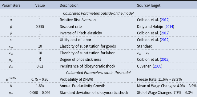
Notes: The table presents the calibration of the model. Parameters are chosen to be as standard as possible to ensure the results are comparable to the existing literature. Three parameters are calibrated to match the empirical wage change distributions; this table presents the calibration for both specifications used in the paper.
Bils and Klenow (Reference Bils and Klenow2004) estimate that firms reset prices every 4 to 5 months and Nakamura and Steinsson (Reference Nakamura and Steinsson2008) find that firms change prices every 9 to 11 months.Footnote 23 In accordance with Coibion et al. (Reference Coibion, Gorodnichenko and Wieland2012), I choose the middle of this range (7 months) and set the degree of price stickiness accordingly. In fact, this parameter is crucial to the analysis, as its impact on the cost of inflation is highlighted in Nakamura et al. (Reference Nakamura, Steinsson, Sun and Villar2018). Consequently, one side of the trade-off (sand-effect) in the paper depends on the choice of this parameter. To address this, I provide a robustness exercise examining the impact of this side.
I calibrate the model using two different specifications. In the first specification, to match the wage freeze rate of 11.6% in the annual total wage change distribution, $\mu ^{\text{DNWR}}$
is calibrated to 0.75, and to match the second moment of the distribution,
$\mu ^{\text{DNWR}}$
is calibrated to 0.75, and to match the second moment of the distribution, $\sigma _q$
is set to 0.06. In the second specification, to match the wage freeze rate of 33.2% in the base wage change distribution,
$\sigma _q$
is set to 0.06. In the second specification, to match the wage freeze rate of 33.2% in the base wage change distribution, $\mu ^{\text{DNWR}}$
is calibrated to 0.95, and
$\mu ^{\text{DNWR}}$
is calibrated to 0.95, and $\sigma _q$
is set to 0.066. To accurately match the mean of wage changes, the productivity growth rate is set to 1.6% per year, which is approximately the average annualized labor productivity growth over 2008–2019.Footnote
24
To facilitate comparison with Coibion et al. (Reference Coibion, Gorodnichenko and Wieland2012), all parameters except for productivity growth are taken directly from that paper, including the use of log utility for consumption. The Frisch elasticity parameter is set to 1.Footnote
25
The elasticity of substitution between goods and labor is assumed to be equal and set to 10, implying a markup of 11%. The persistence of idiosyncratic productivity shock is taken from Guvenen (Reference Guvenen2009).Footnote
26
The standard deviation of idiosyncratic shocks is calibrated to match the standard deviation of the wage change distribution.Footnote
27
The annual discounting in the model is assumed to be 2%, following Daly and Hobijn (Reference Daly and Hobijn2014). Therefore, the quarterly discount rate is set to 0.995.
$\sigma _q$
is set to 0.066. To accurately match the mean of wage changes, the productivity growth rate is set to 1.6% per year, which is approximately the average annualized labor productivity growth over 2008–2019.Footnote
24
To facilitate comparison with Coibion et al. (Reference Coibion, Gorodnichenko and Wieland2012), all parameters except for productivity growth are taken directly from that paper, including the use of log utility for consumption. The Frisch elasticity parameter is set to 1.Footnote
25
The elasticity of substitution between goods and labor is assumed to be equal and set to 10, implying a markup of 11%. The persistence of idiosyncratic productivity shock is taken from Guvenen (Reference Guvenen2009).Footnote
26
The standard deviation of idiosyncratic shocks is calibrated to match the standard deviation of the wage change distribution.Footnote
27
The annual discounting in the model is assumed to be 2%, following Daly and Hobijn (Reference Daly and Hobijn2014). Therefore, the quarterly discount rate is set to 0.995.
Using this set of parameters, I calculate welfare for various steady-state inflation rates. Two primary channels significantly influence welfare in this analysis: (1) the presence of DNWR, which reduces labor supply and is mitigated by a higher inflation target (the “greasing” effect), and (2) price stickiness, which creates economic distortions through increased price dispersion at higher inflation rates (the “sand” effect).Footnote 28
To facilitate welfare comparisons, I first calculate welfare for a flex-price economy–where prices and wages are fully flexible–as the benchmark case. I then measure welfare losses in economies with DNWR constraints and/or price rigidity as deviations from the benchmark economy across different trend inflation rates. These welfare losses are expressed in terms of consumption equivalence.
 \begin{align*} ln(\lambda C^n)-\omega \left (\Sigma _{i=1}^{N_w} \Sigma _{j=1}^{N_{q}} F_{i, j}^n \frac {{l_{i, j}^n}^{(1+\psi)}}{(1+\psi)}\right) = ln( C)-\omega \left (\Sigma _{i=1}^{N_w} \Sigma _{j=1}^{N_{q}} F_{i, j} \frac {l_{i, j}^{(1+\psi)}}{(1+\psi)}\right) \end{align*}
In this equation, the benchmark scenario is indicated with a superscript “n” (natural level), and “F” represents the stationary distribution over the wage and productivity space, which act as state variables in the model. I calculate the values of $\lambda$
(consumption equivalence), which reflect the welfare cost of deviations from the flex-price and flex-wage case, for various model specifications.
$\lambda$
(consumption equivalence), which reflect the welfare cost of deviations from the flex-price and flex-wage case, for various model specifications.
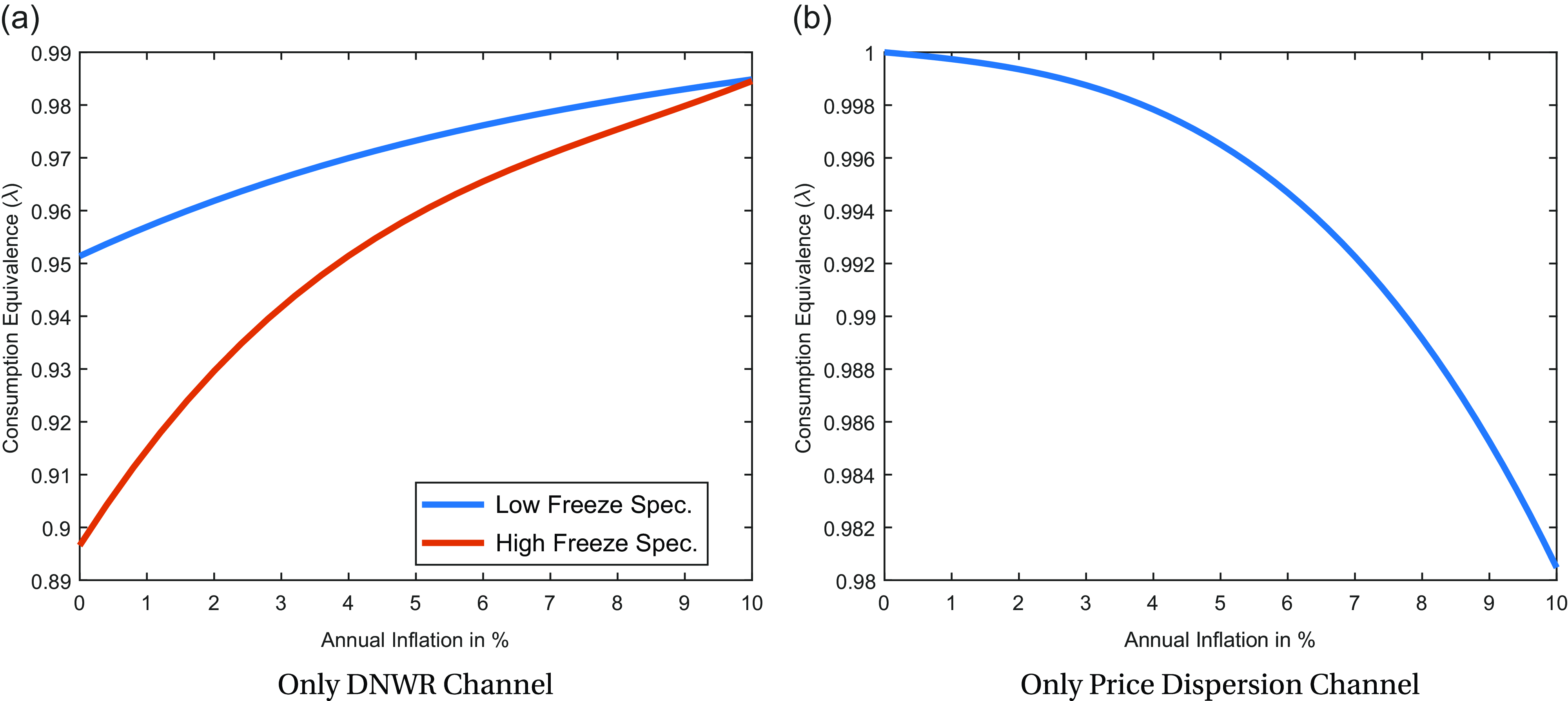
Figure 2. Welfare costs of DNWR and sticky prices, separately.
Notes: The figure plots consumption-equivalent welfare for each specification as a function of the inflation rate, relative to welfare in a fully flexible price and wage setting. It quantifies distortions in the labor market and goods market separately, highlighting the trade-off between these two key channels. At inflation rates close to zero, the welfare cost of DNWR is approximately 5% when the low freeze rate is matched and 10% when the high freeze rate is matched.
As documented in Figure-2a, the DNWR constraint becomes less costly as the inflation rate increases, due to the decreasing wage freeze rate (also known as the “grease effect”). Although the relationship is not perfectly linear, increasing trend inflation by 1 percentage point improves consumption-equivalent welfare by approximately 0.3 percentage points. Under the high freeze rate specification, this improvement is more pronounced, reaching nearly 0.8 percentage points. This finding indicates that raising the inflation target alleviates the welfare cost of DNWR by reducing distortions in the labor market. In standard models, staggered wage contracts are very costly under positive trend inflation (Ascari et al. Reference Ascari, Phaneuf and Sims2018).Footnote 29 In my model, the asymmetry in staggered wage contracts–where wages are flexible upward but rigid downward–leads to a reduction in welfare costs as inflation increases.
Under flexible wages, the wage change distribution would follow a normal distribution, as the idiosyncratic productivity shock is modeled as a Gaussian process, with wages adjusting to reflect productivity. In this scenario, there are no distortions in the labor market, and deviations from the flexible price-wage benchmark arise solely due to increased price stickiness at positive trend inflation rates. The associated welfare cost is depicted in Figure-2b. Furthermore, in the absence of heterogeneity and aggregate uncertainty, DNWR would not bind for representative agents, resulting in no costs associated with DNWR. The same graph would be obtained in such a setting, as inefficiencies would arise exclusively from the “sand effect.”
In short, Figure-2b shows that welfare costs increase with higher inflation under price stickiness due to greater price dispersion and inefficient price allocation, with no distortions originating from the labor market. The distortive impact of price dispersion arises because, when a firm has the opportunity to reset its price, it must overadjust to account for trend inflation over the expected duration during which it cannot change the price again. This overadjustment becomes increasingly pronounced with greater price stickiness and higher trend inflation. If price stickiness is the only friction, without a DNWR constraint, the optimal inflation rate would be 0%, consistent with the standard implication of a New Keynesian model.
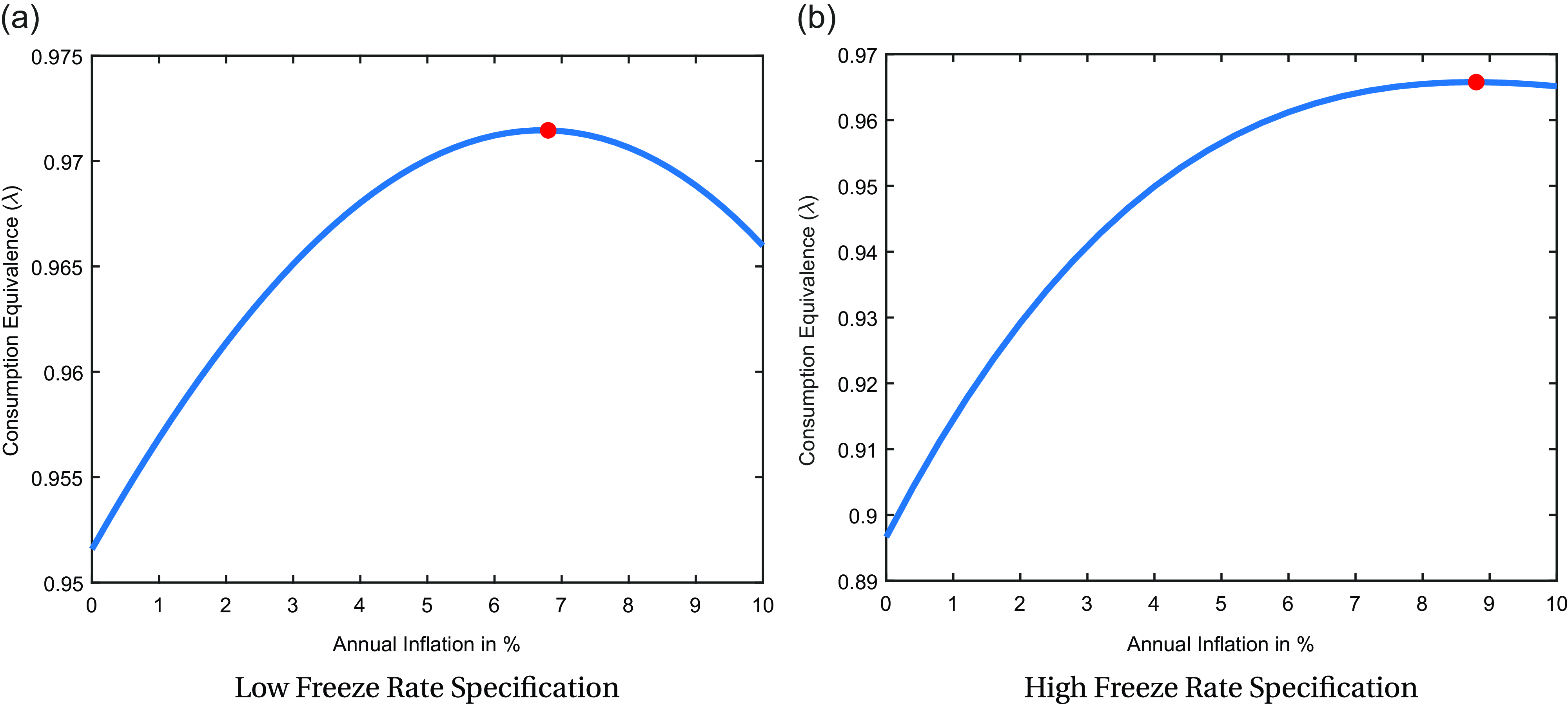
Figure 3. Welfare cost of DNWR and sticky prices at different steady-state inflation rates.
Notes: The figure plots the consumption-equivalent welfare as a function of the inflation rate, relative to welfare under completely flexible prices. Both the DNWR channel and the price stickiness channel are active in this analysis. The red circle indicates the peak of the curve. Panel (a) presents the results for the specification where the annual total wage change distribution is matched, while Panel (b) shows the results for the specification where the annual base wage change distribution is matched. This figure quantifies the trade-off between these channels and indicates that the optimal inflation target is 6.8% for the low freeze rate (11.6%) case and 8.8% for the high freeze rate (33.2%).
Combining these two channels, Figure-3 illustrates which channel dominates for each specification. With both channels active, the optimal steady-state inflation rate is found to be 6.8% when total wage change distribution is matched and found to be 8.8% when base wage change distribution is matched.Footnote 30 Figure-C8 shows that the optimal rates drop to 4.8% and 6.0%, respectively, if a higher price stickiness is assumed, with a price duration of 9 months instead of 7 months. However, since prices become more flexible with a higher inflation rate, this is not a likely scenario (Alvarez et al. Reference Alvarez, Beraja, Gonzalez-Rozada and Neumeyer2018), and thus these rates may represent the most conservative estimates in this exercise. Overall, the optimal rates in this analysis are relatively high compared to previous literature, highlighting the importance of the DNWR channel. This finding contrasts with the conclusions drawn by Coibion et al. (Reference Coibion, Gorodnichenko and Wieland2012), who, using a representative agent model, argue that DNWR occasionally binds for aggregate wages and does not play a significant role. In fact, the existence of DNWR can even be beneficial and, in some specifications, may reduce the optimal inflation target by decreasing the binding frequency of the zero lower bound (ZLB) (Billi and Galí, Reference Billi and Galí2020; Amano and Gnocchi, Reference Amano and Gnocchi2023). However, the analysis shows that when DNWR binds at the individual level, it can create significant distortions in the labor market. Consequently, reducing the binding rate of DNWR through higher inflation could lead to substantial welfare improvements. It also differs from the estimates by Fagan and Messina (Reference Fagan and Messina2009) and Mineyama (Reference Mineyama2022), which employ variants of the menu-cost model in a heterogeneous agent setting.Footnote 31 In the present model, there are always some households who are constrained by DNWR and they cannot set the optimal wages they would like to set in the absence of the DNWR constraint.Footnote 32 As a result, the DNWR channel alone significantly increases the optimal inflation rate.Footnote 33 Setting the inflation target at 6.8% instead of 2% results in a welfare gain of 1.10 percentage points in consumption equivalence, while raising the rate to 8.8% leads to a much larger gain of nearly 3.60 percentage points, which can be considered as the upper bound in this analysis.
Next, Figure-4a illustrates the significance of the wage freeze rate on the optimal inflation target. When the wage freeze rate is high, reflecting the inability to adjust wages optimally, the associated welfare cost also rises. By varying the DNWR parameter, the wage freeze rate can be changed and the corresponding optimal inflation rates can be determined. As expected, with a higher DNWR parameter, $\mu ^{DNWR}$
, the wage freeze rate increases. Keeping all other parameters constant,
$\mu ^{DNWR}$
, the wage freeze rate increases. Keeping all other parameters constant, $\mu ^{DNWR}$
is calibrated to modify the wage freeze rate in the distribution, and its effect on the optimal inflation rate is documented. A higher
$\mu ^{DNWR}$
is calibrated to modify the wage freeze rate in the distribution, and its effect on the optimal inflation rate is documented. A higher $\mu ^{DNWR}$
also raises the binding rate of the DNWR constraint, resulting in greater labor market distortions and pushing the optimal inflation rate even higher.
$\mu ^{DNWR}$
also raises the binding rate of the DNWR constraint, resulting in greater labor market distortions and pushing the optimal inflation rate even higher.
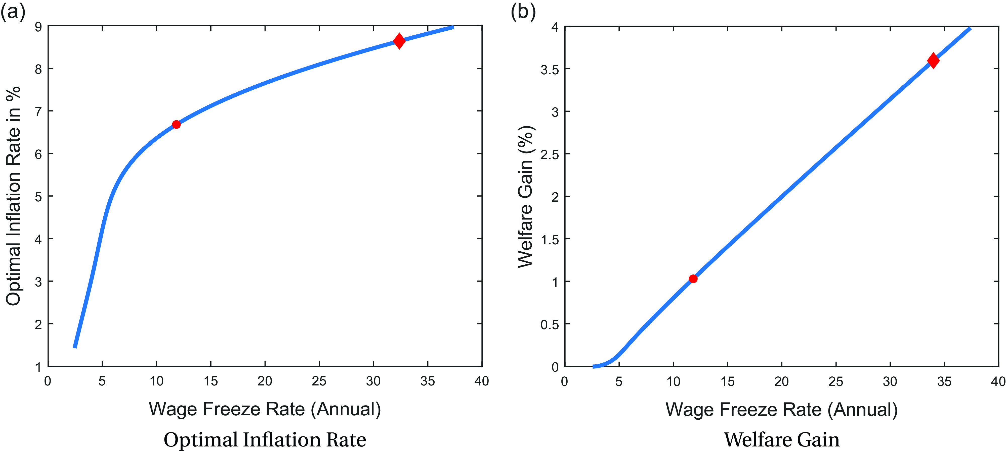
Figure 4. Optimal steady state inflation and welfare gain.
Notes: The figure illustrates the optimal inflation rate as a function of the wage freeze rate and compares the welfare gain achieved by setting the inflation rate to the optimal level for each wage freeze rate against the 2% target economy. When the wage freeze rate in the wage change distribution is 11.6%, the optimal inflation rate is approximately 6.8%, with a corresponding welfare gain of 1.1%, represented by a red circle. For a wage freeze rate of 33.2%, the optimal inflation rate increases to 8.8%, with a corresponding welfare gain of 3.6%, represented by a red diamond. The parameter $\mu ^{DNWR}$
is recalibrated to adjust the wage freeze rate in the analysis.
$\mu ^{DNWR}$
is recalibrated to adjust the wage freeze rate in the analysis.
The results suggest that for extreme levels of wage freeze rates (37%), the optimal inflation target can reach as high as 9%. This indicates that when nominal wage cuts are entirely restricted ( $\mu ^{DNWR} = 1$
), an optimal inflation rate of approximately 9% provides sufficient flexibility for real wage reductions when necessary. Given that empirical distributions show an annual wage freeze rate of 11.6% and a base wage freeze rate of 33.2%, the optimal inflation target should range between 6.8% and 8.8%, as indicated by the two red dots in the graph.
$\mu ^{DNWR} = 1$
), an optimal inflation rate of approximately 9% provides sufficient flexibility for real wage reductions when necessary. Given that empirical distributions show an annual wage freeze rate of 11.6% and a base wage freeze rate of 33.2%, the optimal inflation target should range between 6.8% and 8.8%, as indicated by the two red dots in the graph.
Figure-4b documents the welfare gain if the inflation target is set to the optimal level based on the economy’s wage freeze rate. It demonstrates how the optimal inflation target at different wage freeze rates improves welfare, compared to an economy with a 2% inflation target, in terms of consumption equivalence, using the optimal inflation rates documented above. If the wage freeze rate is low in an economy, the improvement in welfare from setting the inflation target to the optimal rate is minimal. However, as the wage freeze rate increases, adjusting the target to the optimal level becomes more important due to the higher welfare gains. In the case of the U.S. economy, where the wage freeze rate for the total wage changes is 11.6%, setting the inflation target to the optimal rate of 6.8% instead of 2% results in a welfare gain of 1.10 percentage points in terms of consumption equivalence. Considering the rise in wage freeze rates since the 1980s, the welfare cost of this labor market friction also increases over time if the target remains at 2%. In the case of a 33.2% wage freeze rate for the base wage change distribution, raising the target to higher levels can result in a welfare improvement exceeding 3.5 percentage points in terms of consumption equivalence, which represents a substantial welfare gain by standard measures in the literature.
5. Sensitivity analysis and robustness check
The model suggests that the steady-state inflation rate should be between 6.8% and 8.8%; however, it is essential to verify whether this result is sensitive to the calibrated parameters. Variations in parameter choices could influence the costs associated with the DNWR channel or the price stickiness channel, potentially altering the optimal inflation rate. In this section, to provide conservative estimates, I use the low freeze rate specification as the benchmark and examine all possible variations in the parameterization of the model.
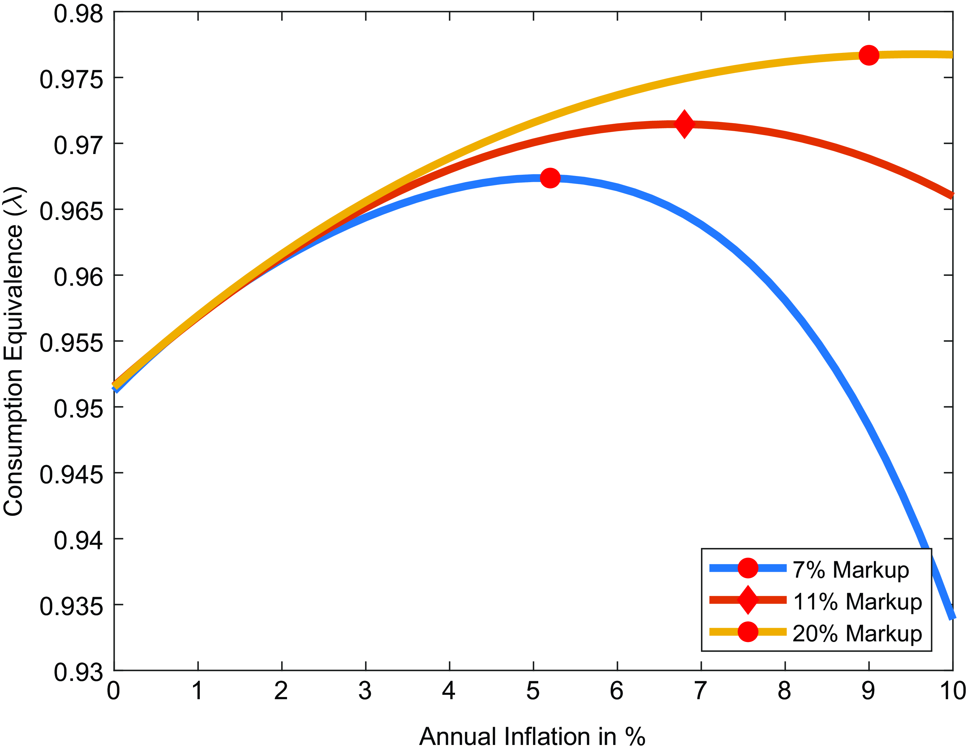
Figure 5. Optimal inflation rate, markup.
Notes: The figure plots the consumption-equivalent welfare of economies with different markup rates as a function of the inflation rate relative to welfare when prices are fully flexible. Diamond shape indicates the benchmark case.
In Figure-5, the price elasticity parameter is analyzed. I decrease the parameter to 6 such that markup has increased from 11% to 20%, which is in line with the recent literature about increasing markups (De Loecker et al. Reference De Loecker, Eeckhout and Unger2020). Consistent with the literature,Footnote 34 the welfare cost of price stickiness is higher with a higher elasticity of substitution between intermediate goods (lower markup), as demand is more elastic to price changes, increasing goods market misallocations due to price rigidity. Consequently, with a higher markup, the optimal inflation rate is higher as well. To be more conservative in estimating the optimal target, I assume an elasticity of substitution of 10 (markup of 11%) instead of 6 (markup of 20%) in the benchmark case.
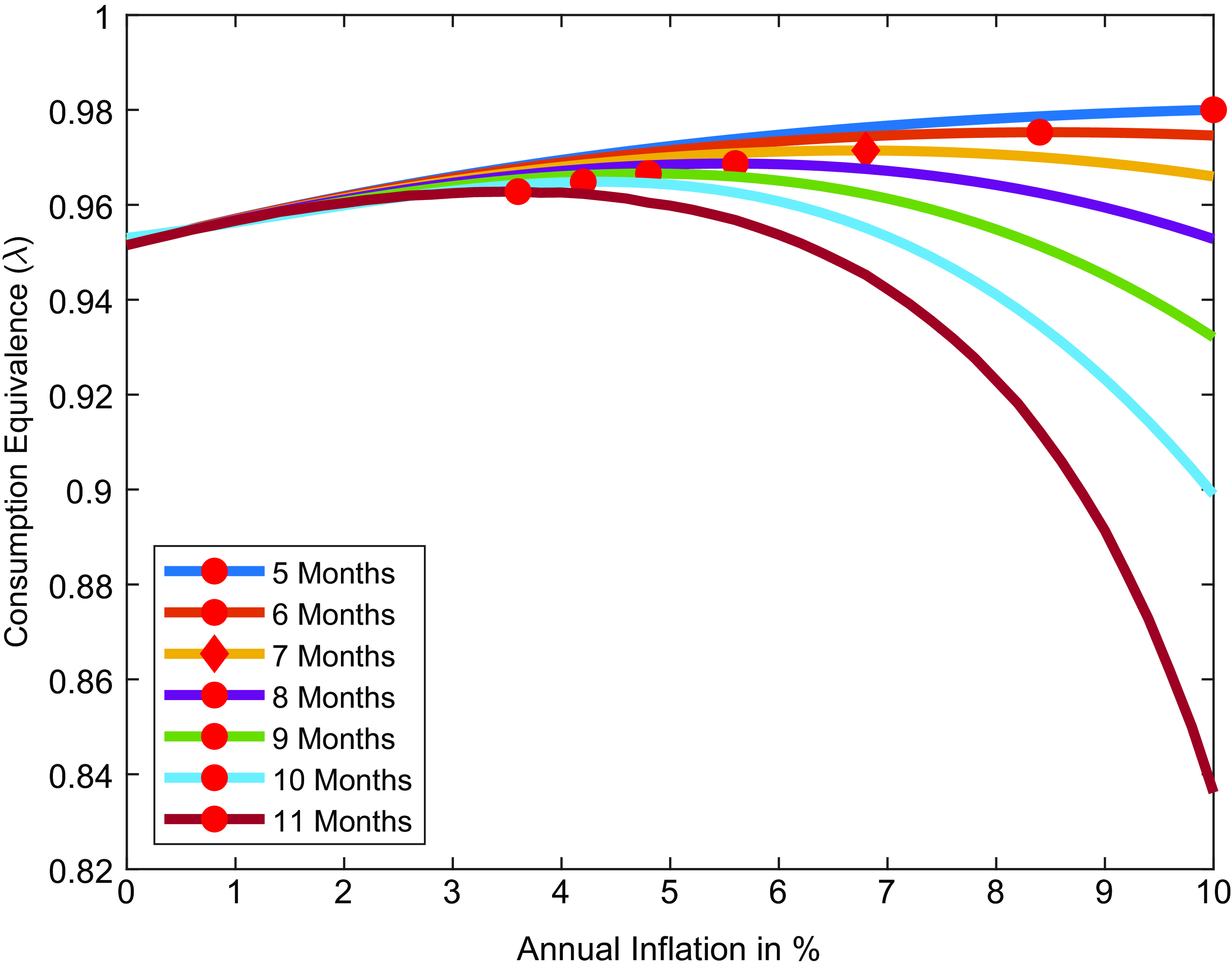
Figure 6. Optimal inflation rate, price stickiness $\mu _p$
.
$\mu _p$
.
Notes: The figure plots the consumption-equivalent welfare of economies with different price stickiness level as a function of the inflation rate relative to welfare when prices are completely flexible. Diamond shape indicates the benchmark case.
The more flexible prices are, the lower the welfare cost of inflation. As shown in Figure-6, the optimal inflation rate increases with more flexible prices, as the DNWR channel becomes dominant. Price stickiness primarily affects the price-setting decisions of firms but does not impact the wage-setting process. As a result, changes to the price stickiness parameter influence price dispersion without altering the cost associated with the wage-setting process, as seen in equations (4)–(6). When a firm resets its price, it needs to set it higher than necessary to account for the anticipated inflation over the period during which it expects to be unable to adjust the price again. This overadjustment becomes more pronounced with greater price stickiness (higher $\mu _{p}$
) and higher trend inflation, leading to increased price dispersion and a more inefficient allocation of prices. Consequently, the optimal inflation rate decreases as the stickiness parameter increases.
$\mu _{p}$
) and higher trend inflation, leading to increased price dispersion and a more inefficient allocation of prices. Consequently, the optimal inflation rate decreases as the stickiness parameter increases.
Bils and Klenow (Reference Bils and Klenow2004) estimate that firms reset prices every 4 to 5 months, suggesting that the optimal inflation rate under such conditions could be as high as 10%. On the other hand, Nakamura and Steinsson (Reference Nakamura and Steinsson2008) estimate that firms change prices every 8 to 11 months when considering regular prices, with the inclusion of product substitutions reducing the implied duration to 7 to 9 months. The 11-month duration for regular prices represents the upper bound of estimates in the literature. Even under this assumption, the optimal inflation target exceeds 3%, reaching approximately 3.6%.
However, as inflation rises, the frequency of price changes increases, as documented by Alvarez et al. (Reference Alvarez, Beraja, Gonzalez-Rozada and Neumeyer2018). This suggests that in an inflationary environment, prices are unlikely to remain highly sticky. Consequently, the cost of price dispersion associated with higher inflation is further reduced when prices change more frequently, as shown by Levin and Yun (Reference Levin and Yun2007) and Nakamura et al. (Reference Nakamura, Steinsson, Sun and Villar2018). The baseline calibration adopted here strikes a balance between the high and low-end estimates in the literature, consistent with Coibion et al. (Reference Coibion, Gorodnichenko and Wieland2012).

Figure 7. Optimal inflation rate, (Inverse) frisch elasticity $\psi$
.
$\psi$
.
Notes: The figure plots the consumption-equivalent welfare of economies with different Frisch elasticities as a function of the inflation rate relative to welfare when prices are completely flexible. Diamond shape indicates the benchmark case.
In Figure-7, I analyze variation in the levels of the (inverse) Frisch labor supply elasticity. I opt to use a conservative estimate for Frisch elasticity ( $\psi =1$
) for the benchmark case but if I increase it further, the optimal inflation target increases because labor supply becomes more inelastic with respect to wage and thus the cost of DNWR is higher.Footnote
35
A higher value of
$\psi =1$
) for the benchmark case but if I increase it further, the optimal inflation target increases because labor supply becomes more inelastic with respect to wage and thus the cost of DNWR is higher.Footnote
35
A higher value of $\psi$
implies that the disutility from labor supply is more convex, leading to greater welfare losses due to inefficient wage setting.
$\psi$
implies that the disutility from labor supply is more convex, leading to greater welfare losses due to inefficient wage setting.
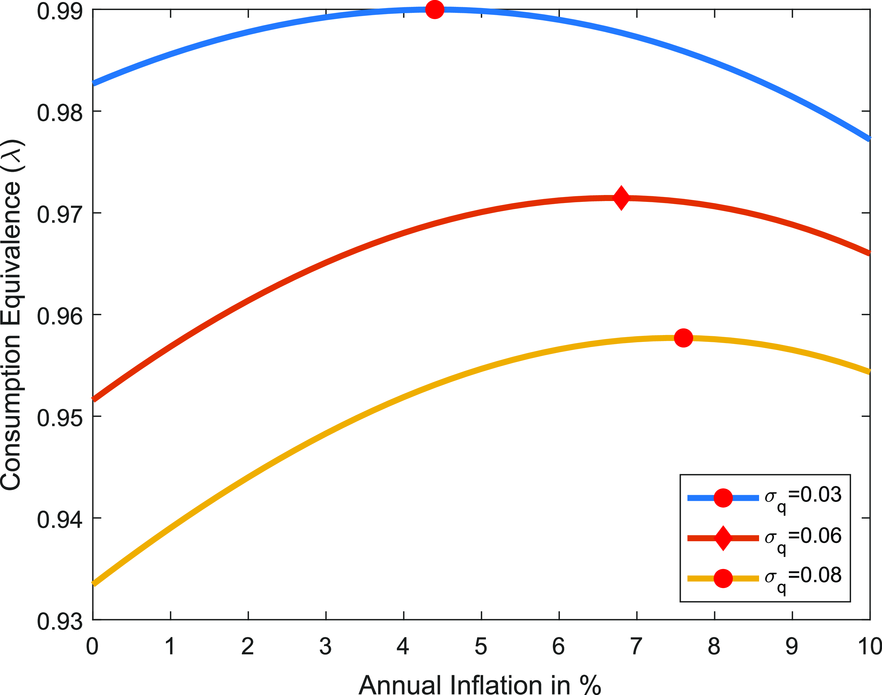
Figure 8. Optimal inflation rate, std of productivity $\sigma _{q}$
.
$\sigma _{q}$
.
Notes: The figure plots the consumption-equivalent welfare of economies with different Frisch elasticities as a function of the inflation rate relative to welfare when prices are completely flexible. Diamond shape indicates the benchmark case.
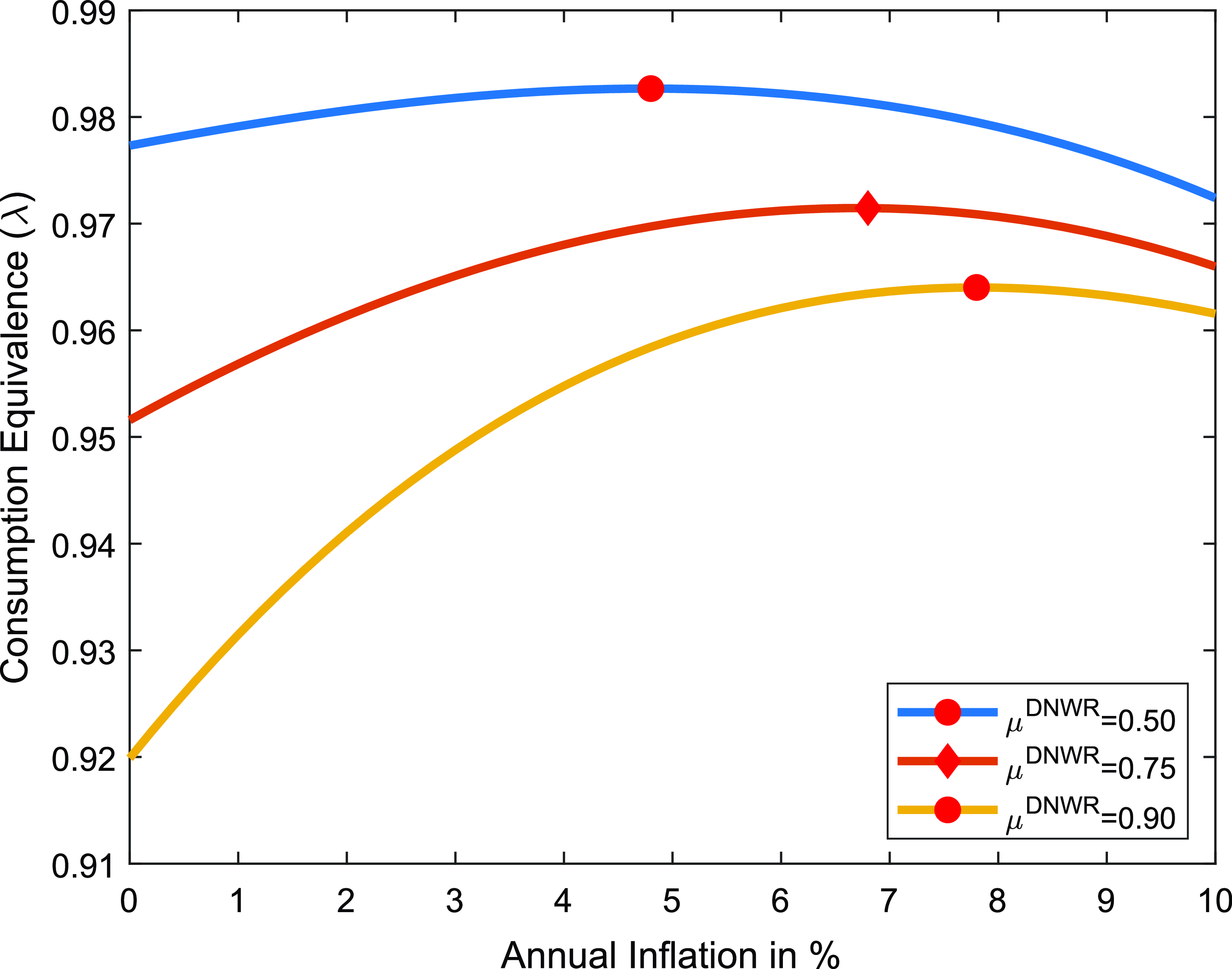
Figure 9. Optimal inflation rate, DWNR parameter $\mu ^{DNWR}$
.
$\mu ^{DNWR}$
.
Notes: The figure plots the consumption-equivalent welfare of economies with different DNWR parameter as a function of the inflation rate relative to welfare when prices are completely flexible. Diamond shape indicates the benchmark case.
Since the distortionary impact of DNWR on labor supply is more costly when the labor supply elasticity is lower, a higher value of $\psi$
–which corresponds to a lower Frisch elasticity–results in greater welfare costs associated with the DNWR channel. This shift increases the optimal inflation rate. The Frisch elasticity is a critical parameter in this analysis, and as shown in Figure-7, the main findings are robust to variations in this parameter.
$\psi$
–which corresponds to a lower Frisch elasticity–results in greater welfare costs associated with the DNWR channel. This shift increases the optimal inflation rate. The Frisch elasticity is a critical parameter in this analysis, and as shown in Figure-7, the main findings are robust to variations in this parameter.
In Figure-8, I calculate the optimal inflation rate as the standard deviation of the shock process varies. As a result, I observe a less (more) dispersed wage change distribution with a lower (higher) wage freeze rate, leading to lower (higher) welfare costs stemming from the DNWR channel. Even if the standard deviation is reduced by half, the welfare cost due to the DNWR constraint remains high: the estimated optimal trend inflation is 4.4%, significantly higher than the current target of 2%.
Finally, the parameter representing the degree of downward wage rigidity, denoted by $\mu ^{DNWR}$
, plays a crucial role in determining the welfare cost associated with such rigidity, as illustrated in Figure-9. A higher value of
$\mu ^{DNWR}$
, plays a crucial role in determining the welfare cost associated with such rigidity, as illustrated in Figure-9. A higher value of $\mu ^{DNWR}$
implies a higher wage freeze rate, resulting in a more rigidity on wages and a higher degree of distortion in the labor market. Consequently, the optimal inflation rate shifts to the right, potentially reaching as high as 8%. Since the empirical estimates show that the wage freeze rate in the U.S. is around 11.6%, the paper suggests that the inflation targeting should be set as high as 7% to promote a more flexible labor market and lower the long-run unemployment rate.Footnote
36
Even if a low level of downward rigidity is assumed, the optimal inflation target would still need to be higher than 4.5%.Footnote
37
$\mu ^{DNWR}$
implies a higher wage freeze rate, resulting in a more rigidity on wages and a higher degree of distortion in the labor market. Consequently, the optimal inflation rate shifts to the right, potentially reaching as high as 8%. Since the empirical estimates show that the wage freeze rate in the U.S. is around 11.6%, the paper suggests that the inflation targeting should be set as high as 7% to promote a more flexible labor market and lower the long-run unemployment rate.Footnote
36
Even if a low level of downward rigidity is assumed, the optimal inflation target would still need to be higher than 4.5%.Footnote
37
6. Asymmetric menu cost model
Now, instead of modeling with Calvo type wage setting process, I introduce DNWR with asymmetric menu cost pricing. For that, I focus solely on base earnings as in Grigsby et al. (Reference Grigsby, Hurst and Yildirmaz2021) and match moments accordingly. The wage-setting part of the model has been changed to integrate menu cost as follows:
 \begin{align*} \text{if } w_t^*(i) \geq \frac {w_{t-1}(i)}{\pi _t A_t} \quad \begin{cases} w_t(i)=w_t^*(i) \text{ and no cost}, \end{cases} \end{align*}
 \begin{align*} \text{if } w_t^*(i) \lt \frac {w_{t-1}(i)}{\pi _t A_t} \quad \begin{cases} w_t(i)=w_t^*(i) \text{ and pays $\Psi $}. \end{cases} \end{align*}
Here, $w_t^*$
is the optimal real wage of households. Households are free to adjust their wages upward nominally, but they incur a utility cost
$w_t^*$
is the optimal real wage of households. Households are free to adjust their wages upward nominally, but they incur a utility cost $\Psi$
if the adjustment is nominally downward. The calibration remains the same as in the benchmark case; the only difference is that the menu cost parameter
$\Psi$
if the adjustment is nominally downward. The calibration remains the same as in the benchmark case; the only difference is that the menu cost parameter $\Psi$
is set to 1.145 to match the wage freeze rate in the base wage change distribution, replacing the
$\Psi$
is set to 1.145 to match the wage freeze rate in the base wage change distribution, replacing the $\mu ^{\text{DNWR}}$
parameter. Additionally,
$\mu ^{\text{DNWR}}$
parameter. Additionally, $\sigma _q$
is slightly adjusted to 0.063 to match the standard deviation of the distribution accurately.
$\sigma _q$
is slightly adjusted to 0.063 to match the standard deviation of the distribution accurately.
Figure-10 demonstrates that incorporating DNWR through an asymmetric menu cost model yields the same optimal inflation rate of 8.8% when the empirical base wage change distribution is accurately matched. This finding underscores the robustness of the results, as moving from an asymmetric Calvo-type wage-setting model to an asymmetric menu-cost framework does not lead to significant differences, provided that the wage change distribution is accurately captured. Notably, the welfare cost of DNWR under the menu-cost model is smaller than that under the Calvo-type model at low inflation targets. Furthermore, while the welfare cost declines as the inflation rate increases, this decline occurs more rapidly in the Calvo-type framework. The reason for this is that, at higher inflation rates, the menu-cost approach still incurs the utility cost of $\Psi$
for nominal wage reductions. In contrast, under the Calvo-type framework, the DNWR constraint is unlikely to bind at higher inflation rates, resulting in minimal costs. Overall, both approaches suggest the same optimal trend inflation rate.
$\Psi$
for nominal wage reductions. In contrast, under the Calvo-type framework, the DNWR constraint is unlikely to bind at higher inflation rates, resulting in minimal costs. Overall, both approaches suggest the same optimal trend inflation rate.

Figure 10. Welfare cost of DNWR modeled with asymmetric menu cost.
Notes: The figure plots the consumption-equivalent welfare as a function of the inflation rate, relative to welfare when prices are completely flexible. In this case, DNWR is modeled using an asymmetric menu-cost type wage setting, rather than an asymmetric Calvo-type wage setting. The red circle indicates the peak of the curve. This figure quantifies the trade-off between these channels and suggests that the optimal inflation target should be 8.8%.
However, this result is higher than those reported in other studies that use models with menu-type wage-setting to reflect the DNWR constraint (Mineyama, Reference Mineyama2023; Fagan and Messina, Reference Fagan and Messina2009). To ensure comparability with Mineyama (Reference Mineyama2023), I calibrate the economy by directly adopting all relevant parameters.Footnote 38 The asymmetric menu cost model employed here is admittedly a simplified version of the menu cost wage-setting model used in Mineyama (Reference Mineyama2022). However, it sufficiently captures the moments of the base wage change distribution with accuracy.
The parameterization in this model differs significantly, as shown in Table-3. First, setting $\psi = 0.5$
significantly reduces the optimal inflation rate, as illustrated in Figure-7 before. This is because a less convex disutility from labor supply reduces the welfare cost of DNWR.Footnote
39
Additionally, the relatively low elasticity of substitution for labor (
$\psi = 0.5$
significantly reduces the optimal inflation rate, as illustrated in Figure-7 before. This is because a less convex disutility from labor supply reduces the welfare cost of DNWR.Footnote
39
Additionally, the relatively low elasticity of substitution for labor ( $\epsilon _w = 3.5$
) in this calibration, compared to values typically used in the literature,Footnote
40
further decreases the optimal inflation rate. As demonstrated in Figure-C5, the distortionary impact of DNWR diminishes with lower
$\epsilon _w = 3.5$
) in this calibration, compared to values typically used in the literature,Footnote
40
further decreases the optimal inflation rate. As demonstrated in Figure-C5, the distortionary impact of DNWR diminishes with lower $\epsilon _w$
, as higher elasticity of substitution amplifies the welfare cost of wage stickiness. Since
$\epsilon _w$
, as higher elasticity of substitution amplifies the welfare cost of wage stickiness. Since $\epsilon _w=3.5$
implies a 40% markup, I adopt
$\epsilon _w=3.5$
implies a 40% markup, I adopt $\epsilon _w=10$
in my benchmark specification to align with standard New Keynesian models.
$\epsilon _w=10$
in my benchmark specification to align with standard New Keynesian models.
Table 3. Parameterization of the model
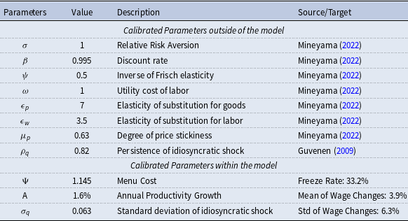
Notes: The parameters are now chosen directly from Mineyama (Reference Mineyama2022) to ensure that the results are comparable to those in the paper. Three parameters are calibrated to match the empirical wage change distribution.
Table-4 shows that introducing the asymmetric menu cost wage setting into the model allows it to accurately capture the empirical distribution, both with the benchmark model presented above and with the model that adopts all parameters directly from Mineyama (Reference Mineyama2022).
Table 4. Targeted and untargeted moments

Notes: The table presents the model results for the asymmetric menu cost in wage setting to match the empirical moments, as well as the model results calibrated directly with parameters from Mineyama (Reference Mineyama2022) for comparability with that paper. The parameters $\Psi, A, \sigma _q$
are calibrated to match these moments.
$\Psi, A, \sigma _q$
are calibrated to match these moments.
In the benchmark case, the optimal rate remains nearly the same, indicating that modeling the wage setting mechanism through either asymmetric Calvo-type or asymmetric menu cost wage setting does not lead to a significant difference, as long as the empirical distribution is matched accurately. However, Mineyama (Reference Mineyama2022) suggests a lower inflation rate, and the analysis below shows that the choice of parameter set is the primary driver of this difference.

Figure 11. Welfare cost of DNWR modeled with asymmetric menu cost.
Notes: The figure plots the wage change distribution at different frequencies. The model is run quarterly and the distribution is then annualized to match the empirical one. The wage freeze rate, mean and standard deviation of wage changes are targeted moments.
Although prices are slightly stickier in this specification, the combined effects of the two parameters–lower Inverse Frisch elasticity ( $\Psi$
) and lower elasticity of substitution for labor (
$\Psi$
) and lower elasticity of substitution for labor ( $\epsilon _w$
)–dominate, leading to a substantial reduction in the optimal inflation rate. As shown in Figure-11, the optimal inflation rate under this calibration is approximately 3.2%. This slightly higher rate results from the adoption of a different version of menu cost-type wage setting in (Mineyama, Reference Mineyama2022), as well as the inclusion of 5% of job changers who can freely adjust their wages, further reducing the optimal rate.Footnote
41
Overall, this analysis highlights why the results differ in this setting: the parameterization plays a crucial role in determining the strength of the DNWR constraint.
$\epsilon _w$
)–dominate, leading to a substantial reduction in the optimal inflation rate. As shown in Figure-11, the optimal inflation rate under this calibration is approximately 3.2%. This slightly higher rate results from the adoption of a different version of menu cost-type wage setting in (Mineyama, Reference Mineyama2022), as well as the inclusion of 5% of job changers who can freely adjust their wages, further reducing the optimal rate.Footnote
41
Overall, this analysis highlights why the results differ in this setting: the parameterization plays a crucial role in determining the strength of the DNWR constraint.
Taking into account all the results and robustness checks, I argue that the DNWR constraint is an important factor to consider when discussing the optimal inflation target. The findings suggest that the absence of wage cuts, coupled with a high freeze rate in the wage change distribution, can be a significant source of inefficiency in the labor market. Allowing for some inflation could help mitigate this inefficiency, although the optimal rate may not need to be as high as 9%, as suggested in the benchmark case. This is because DNWR is not the only factor influencing the optimal inflation target; other important considerations are discussed in Appendix-C.
While the findings do not definitively favor one model over the other, Calvo-type wage setting remains the standard approach in frontier heterogeneous-agent New Keynesian models (Kaplan et al. Reference Kaplan, Moll and Violante2018; Broer et al. Reference Broer, Harbo Hansen, Krusell and Öberg2020; Auclert et al. Reference Auclert, Rognlie and Straub2024). Therefore, adopting an asymmetric version of this mechanism to introduce the DNWR constraint may be an effective way to incorporate DNWR into standard models while ensuring ease of integration.
Lastly, along with these other factors, consumption heterogeneity may play a role in this analysis. In the current model, consumption is fully insured across agents, meaning there is no heterogeneity in consumption–everyone consumes the same amount. While the level of consumption varies due to distortions in the labor market, there is no cross-sectional heterogeneity in consumption itself. Instead, the cross-sectional heterogeneity lies in the labor supply of households, which depends on their productivity level and the wage from the previous period. As discussed in (Mineyama, Reference Mineyama2022), incorporating consumption heterogeneity would likely increase the dispersion in households’ willingness to work, resulting in greater demand for wage adjustments. Under DNWR, this would exacerbate labor market distortions, leading to a higher optimal inflation rate. Incorporating full heterogeneity on the consumption side would make the analysis more comprehensive and realistic. However, it is plausible that such heterogeneity would amplify distortions in the labor market further, thereby increasing the optimal inflation rate. This remains an area for future research.
7. Conclusion
In conclusion, this study underscores the significant costs associated with downward nominal wage rigidity (DNWR). The analysis quantifies the trade-off between the commonly used DNWR constraint in recent macroeconomic models and price stickiness. By employing a slightly modified standard New Keynesian model, the study demonstrates how the DNWR constraint interacts with price stickiness, suggesting that the optimal inflation rate should be between 7% and 9%. A high wage freeze rate (33.2%) in the wage change distribution leads to an optimal inflation rate of up to 8.8%, highlighting the economic importance of the DNWR channel. While inflation also increases price dispersion, the impact of the DNWR channel dominates up to a certain threshold, significantly exceeding the conventional 2% inflation target, as shown in robustness tests. Most notably, the welfare impact is substantial: increasing the inflation target from 2% to 7% can yield a welfare gain of 1.10% when the total wage change distribution is aligned, with the potential to reach as high as 3.60% if the base wage change distribution is considered. Although other channels may also affect the optimal inflation target, this analysis demonstrates the distortive impact of DNWR on the labor market.
The paper argues that raising the inflation target alleviates the prevalence of the DNWR constraint, leading to substantial welfare gains. The DNWR friction, within the standard New Keynesian framework, significantly distorts the labor market and imposes considerable welfare costs. Therefore, the paper emphasizes the importance of incorporating the DNWR channel into macroeconomic models to more accurately capture welfare effects and inform policymaking decisions.
Acknowledgements
I am grateful to Saroj Bhattarai, Olivier Coibion, Stefano Eusepi and other faculty members at the Department of Economics, University of Texas at Austin for their helpful comments and suggestions. I thank them for their comments Chris Sims, Christian Bayer, Pablo Ottonello, Esteban-Rossi Hansberg, Soren Hove Ravn, Keith Kuester, Andrea Ferrero, Sergi Basco, Vahagn Jerbashian, Andrea Raffo, Gaston Navarro, Daniel Villar Vallenas, Julio Davila, Harun Alp, Ayşegül Şahin, Yoon Jo, Amy Handlan, Choongryul Yang, Christoph Görtz, Ayşe Kabukçuoǧlu, Refet Gürkaynak and Gazi Kara, and seminar participants at the Fed Board, University of Oxford, Paris School of Economics, Bank of England, Bank of Canada, University of Sydney, Binghamton University, University of Montreal, University of Birmingham, University of Copenhagen, HEC Paris, University of Barcelona, Higher School of Economics, Sabanci University, Koc University, Bilkent University, Bogazici University and Ozyegin University. All remaining errors are mine.
Appendix - A - Computation of the stationary equilibrium
The solution method is a simple fixed point iteration, which is also presented by Fagan and Messina (Reference Fagan and Messina2009). I discretize the idiosyncratic productivity process using Tauchen’s algorithm. And I approximate the value functions on a state space of a grid of 25 points for productivity and 114 points for wages. The process is implemented as follows:
1. Guess an aggregate hours L.
2. Given L, I solve the households’ wage setting problem using value function iteration.
3. Given the policy function of households, I calculate the stationary distribution over the two state variables (wage and productivity).
4. With the stationary distribution in hand, I calculate the aggregate wage W’ and check if it is equal to steady-state wage, W=W’.
5. Lastly, I update aggregate hours L until the convergence is achieved. If not, return to step 2.
Finally, the derivation of $\Omega$
function can be shown easily. The maximization problem is written as follows:
$\Omega$
function can be shown easily. The maximization problem is written as follows:
 \begin{align*}\max _{\left \{C_{t}(i), B_{t+1}(i), W_{t}(i), l_{t}(i)\right \}} \mathbb{E}_{t} \Sigma _{t=0}^{\infty } \beta ^{t}\left [\frac {C_{t}(i)^{1-\sigma }}{1-\sigma }-\omega \frac {l_{t}(i)^{1+\psi }}{1+\psi } \right] \end{align*}
subject to
 \begin{equation} P_{t} C_{t}(i)+ \mathbb{E}_t Q_{t,t+1} B_{t+1}(i) \leq B_{t}(i)+W_{t}(i) l_{t}(i)+\Pi _{t}, \end{equation}
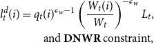 \begin{align} l_{t}^{d}(i)=q_{t}(i)^{\epsilon _w-1}\left (\frac {W_{t}(i)}{W_{t}}\right)^{-\epsilon _w} L_{t}, \\ \text{and }\textbf {DNWR}\text{ constraint,}\nonumber \end{align}
where price of consumption good $P_t$
, unique stochastic discount factor
$P_t$
, unique stochastic discount factor $Q_{t+1}$
and aggregate labor supply
$Q_{t+1}$
and aggregate labor supply $L_t$
are taken as given by households. Since the households’ utility function is additively separable, one can focus on wage-setting part of the problem and I can rewrite their wage setting problem as
$L_t$
are taken as given by households. Since the households’ utility function is additively separable, one can focus on wage-setting part of the problem and I can rewrite their wage setting problem as
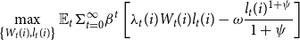 \begin{align*}\max _{\left \{W_{t}(i), l_{t}(i)\right \}} \mathbb{E}_{t} \Sigma _{t=0}^{\infty } \beta ^{t}\left [ \lambda _t(i) W_t(i) l_t(i) - \omega \frac {l_{t}(i)^{1+\psi }}{1+\psi } \right] \end{align*}
subject to
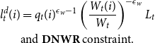 \begin{gather*} l_{t}^{d}(i)=q_{t}(i)^{\epsilon _w-1}\left (\frac {W_{t}(i)}{W_{t}}\right)^{-\epsilon _w} L_{t} \\ \text{and }\textbf {DNWR}\text{ constraint.} \end{gather*}
which constitutes the labor supply choice problem of the households.
Then, the objective function can be expressed by substituting $l_{t}(i)$
with labor demand function (2).
$l_{t}(i)$
with labor demand function (2).
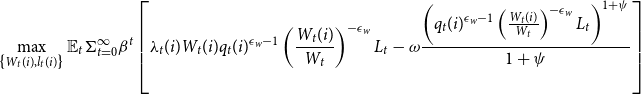 \begin{align*}\max _{\left \{W_{t}(i), l_{t}(i)\right \}} \mathbb{E}_{t} \Sigma _{t=0}^{\infty } \beta ^{t}\left [ \lambda _t(i) W_t(i) q_{t}(i)^{\epsilon _w-1}\left (\frac {W_{t}(i)}{W_{t}}\right)^{-\epsilon _w} L_{t} - \omega \frac {\left (q_{t}(i)^{\epsilon _w-1}\left (\frac {W_{t}(i)}{W_{t}}\right)^{-\epsilon _w} L_{t}\right)^{1+\psi }}{1+\psi } \right] \end{align*}
Since FOC with respect to consumption is $C_t(i)^{-\sigma } = \lambda _t(i) P_t$
, I can write this as
$C_t(i)^{-\sigma } = \lambda _t(i) P_t$
, I can write this as
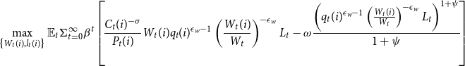 \begin{align*}\max _{\left \{W_{t}(i), l_{t}(i)\right \}} \mathbb{E}_{t} \Sigma _{t=0}^{\infty } \beta ^{t}\left [\! \frac {C_t(i)^{-\sigma }}{P_t(i)} W_t(i) q_{t}(i)^{\epsilon _w-1}\left (\frac {W_{t}(i)}{W_{t}}\right)^{-\epsilon _w} L_{t} - \omega \frac {\left (q_{t}(i)^{\epsilon _w-1}\left (\frac {W_{t}(i)}{W_{t}}\right)^{-\epsilon _w} L_{t}\right)^{1+\psi }}{1+\psi }\! \right] \end{align*}
Because of complete risk-sharing in consumption, consumption is equal to output, $C_t = Y_t=\frac {L}{v_t^p}$
. Then, the whole expression can be simplified to
$C_t = Y_t=\frac {L}{v_t^p}$
. Then, the whole expression can be simplified to
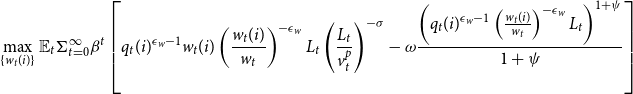 \begin{align*}\max _{\left \{w_{t}(i) \right \}} \mathbb{E}_{t} \Sigma _{t=0}^{\infty } \beta ^{t}\left [ q_{t}(i)^{\epsilon _w-1}w_{t}(i)\left (\frac {w_{t}(i)}{w_{t}}\right)^{-\epsilon _w} L_t \left ( \frac {L_t}{v_t^p} \right)^{-\sigma } - \omega \frac {\left (q_{t}(i)^{\epsilon _w-1}\left (\frac {w_{t}(i)}{w_{t}}\right)^{-\epsilon _w} L_{t}\right)^{1+\psi }}{1+\psi } \right] \end{align*}
which is subject to wage setting (DNWR) constraint and idiosyncratic labor productivity process, given all of the aggregate variables ( $L_t, v_t^p, w_t$
). Here,
$L_t, v_t^p, w_t$
). Here, $w_t$
represents the real detrended aggregate wage,
$w_t$
represents the real detrended aggregate wage, $L_t$
denotes the aggregate labor supply,
$L_t$
denotes the aggregate labor supply, $v_t^p$
is price dispersion. The labor productivity process follows an AR(1) process, while DNWR constraint is defined as asymmetric Calvo type wage setting:
$v_t^p$
is price dispersion. The labor productivity process follows an AR(1) process, while DNWR constraint is defined as asymmetric Calvo type wage setting:
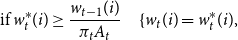 \begin{align*} \text{if } w_t^*(i) \geq \frac {w_{t-1}(i)}{\pi _t A_t} \quad \{w_t(i)=w_t^*(i), \end{align*}
 \begin{align*} \text{if } w_t^*(i) \lt \frac {w_{t-1}(i)}{\pi _t A_t} \quad \begin{cases} w_t(i)=\frac {w_{t-1}(i)}{\pi _t A_t} \quad \text{with the prob } \mu ^{DNWR} \\ w_t(i)=w_t^*(i) \quad \text{with the prob } (1-\mu ^{DNWR}) \end{cases} \end{align*}
where $w_t^*(i)$
is the optimal real wage of an household. For the model with asymmetric Calvo wage setting, the value function is presented in the main text.
$w_t^*(i)$
is the optimal real wage of an household. For the model with asymmetric Calvo wage setting, the value function is presented in the main text.
For the model with asymmetric menu cost type wage setting, the value functions can be written as follows:
 \begin{align*} & V_t(q_t(i),w_{t-1}(i);\;\Gamma _t) \\ & \quad = \left \{ \max _{w_t(i) } \quad \Omega (q_t(i),w_t(i);\;\Gamma _t) - \Psi \mathbf{1} \left (w_t(i) \lt \frac {w_{t-1}(i)}{\pi _t A_t}\right) + \beta \mathbb{E} \left [ V_{t+1} (q_{t+1}(i),w_{t}(i);\;\Gamma _{t+1}) \right] \right \} \end{align*}
where
 \begin{align*} \Omega (q_t(i),w_t(i);\;\Gamma _t)= \left (\! q_{t}(i)^{\epsilon _w-1}w_{t}(i)\left (\frac {w_{t}(i)}{w_{t}}\right)^{-\epsilon _w} L_{t} \left (\frac {L_t}{v_t^p}\right)^{-\sigma }-\omega \frac {\left [q_{t}(i)^{\epsilon _w-1}\left (\frac {w_{t}(i)}{w_{t}}\right)^{-\epsilon _w} L_{t}\!\right]^{1+\psi }}{1+\psi } \right). \end{align*}
The difference in the asymmetric menu cost for wage setting is that, if constrained, households must incur a cost $\Psi \mathbf{1} \left (w_t(i) \lt \frac {w_{t-1}(i)}{\pi _t A_t}\right)$
if they want to revise their wages downward nominally.
$\Psi \mathbf{1} \left (w_t(i) \lt \frac {w_{t-1}(i)}{\pi _t A_t}\right)$
if they want to revise their wages downward nominally.
Appendix - B - Transition dynamics
To analyze transition dynamics, I compute the perfect foresight transition path of the economy in response to a demand (discount rate) shock by following Guerrieri et al. (Reference Guerrieri, Lorenzoni, Straub and Werning2022) and McKay et al. (Reference McKay, Nakamura and Steinsson2016). Specifically, I solve for the response of the model to a one-time unexpected shock to the discount rate. After the initial shock, agents have perfect foresight of all aggregate variables for all periods as the economy returns to the steady state.
First, I assume the economy begins at the steady state and after the shock, it converges back to the steady state over the course of 50 quarters. I initially guess the paths for aggregate labor supply and prices, and then solve for the household’s problem backwards by assuming that the economy will reach the steady state in the final period. Then, I simulate the households forwards using a non-stochastic simulation method (Young, Reference Young2010) and compute wage distribution for each period. With this path of distribution, I calculate the simulated labor supply and prices. If my guess does not provide an equilibrium, I update the aggregate labor supply, prices, and price dispersion. I run the same algorithm again until convergence is achieved. Since there are both aggregate and idiosyncratic non-linearities in the model, the global but computationally costly solution method is the most suitable way to solve the model.Footnote 42
I follow McKay et al. (Reference McKay, Nakamura and Steinsson2016) closely for calculating the transition dynamics.Footnote 43 I use their procedure to find an equilibrium path of the heterogeneous agent model along a perfect foresight transition after receiving a huge demand shock.
I assume that the economy returns to steady-state after T=50 periods. Let X denote a path for all endogenous aggregate variables from date 0 to date T.
 \begin{align*} X \equiv \{ C_t, L_t, N_t, Y_t, v_t^p, w_t, \pi _t, i_t\} \end{align*}
The variables include both aggregate quantities and prices. As an initial guess, I set the values of these variables to steady-state values for the full path. Then, households solve their decision problem, which depends on X.
Given the decision of households, I simulate the population of households to compute updated aggregate labor supply and wage. Here, I use the non-stochastic simulation method of Young (Reference Young2010) and approximate the real wage distribution with 250 equally-spaced bins for each value of productivity. Then, I update the distribution according to households’ decisions. If households choose wages between two binds, I allocate the households to the adjacent bins with some weights by following McKay et al. (Reference McKay, Nakamura and Steinsson2016). With this distribution, I find aggregate labor supply, wage, inflation and price dispersion and check the convergence of these variables. If the tolerance level is not reached, I repeat the process until getting convergence.
We know the Euler equation is:
 \begin{align*} \begin{array}{c} \mathbb{E}_{t}\left [\beta _{t}\left (\frac {L_{t+1}}{L_{t}} \frac {v_{t}^p}{v_{t+1}^p}\right)^{-\sigma } \frac {i_{t}}{\Pi _{t+1}}\right]=1 \end{array} \end{align*}
Fischer rule’s is $ R_t = \frac {i_t}{ \pi _{t+1}}$
and Taylor Rule is simply
$ R_t = \frac {i_t}{ \pi _{t+1}}$
and Taylor Rule is simply $i_t = \frac {\pi _{ss}}{\beta _{ss}}\bigg (\frac {L_t}{L_{ss}}\bigg)^{\Phi _Y}\bigg (\frac {\pi _t}{\pi _{ss}}\bigg)^{\Phi _\pi }$
. From these 3 equations, by dropping expectations I find
$i_t = \frac {\pi _{ss}}{\beta _{ss}}\bigg (\frac {L_t}{L_{ss}}\bigg)^{\Phi _Y}\bigg (\frac {\pi _t}{\pi _{ss}}\bigg)^{\Phi _\pi }$
. From these 3 equations, by dropping expectations I find $L_t$
as:
$L_t$
as:
 \begin{align*} L_t = \bigg ( v_t^p \frac {\beta _t}{\pi _{t+1}} \frac {\pi _{ss}}{\beta _{ss}} \bigg (\frac {\pi _t}{\pi _{ss}}\bigg)^{\Phi _\pi } \bigg (\frac {1}{L_{ss}}\bigg)^{\Phi _Y} \bigg ( \frac {L_{t+1}}{v_{t+1}^p} \bigg)^{-\sigma } \bigg)^\frac {-1}{\sigma +\Phi _Y} \end{align*}
Since I assume in the last period the economy is at steady-state, I get the path of labor supply for 50 periods because I have the inflation given. With inflation, wage and labor supply given I find the policy functions for each period by solving households’ problem. Then, starting with the steady-state distribution, I iterate forward to get labor demand and wage. Lastly, I update wage, inflation and price dispersion with the bisection method.
Following Daly and Hobijn (Reference Daly and Hobijn2014), I analyze the response of the economy to a persistent discount rate shock. Shock magnitude and persistence are selected such that the initial decline in output from the steady state is 10% and the duration of the ZLB is 8 quarters, for the economy with a 2% steady state inflation.Footnote 44 Then, I use the same shock to see how economies with different inflation targets respond to the shock.
Since DNWR is less binding at a higher inflation rate, wages are effectively more flexible and the output gap (unemployment) is lower. The substantial reduction in output as a result of the shock is caused by both the ZLB and DNWR constraints. For economies where the inflation rate is low, the decline is larger and the duration of the ZLB period is longer. As the inflation target rises, the impact of ZLB diminishes and the impact of DNWR decreases due to lower wage freeze rates.
The presence of the ZLB creates a significant output loss, and the ZLB binds less for economies with a relatively high inflation target in this setting. I analyze welfare implications of this result. Here, I use the following formulation for Lucas-type welfare comparison, which is similar to the exercise in the steady-state section.
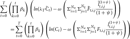 \begin{align*} &\sum _{t=0}^{T} \left ( \prod _{k=0}^{t} \beta _{k} \right) \left ( ln(\lambda _T \tilde {C}_t)-\omega \left (\Sigma _{i=1}^{N_w} \Sigma _{j=1}^{N_{q}} \tilde {F}_{t,i, j} \frac {\tilde {l}_{t,i,j}^{(1+\psi)}}{(1+\psi)}\right) \right)\\ &\qquad = \sum _{t=0}^{T} \left ( \prod _{k=0}^{t} \beta _{k} \right) \left ( ln(C_t)-\omega \left (\Sigma _{i=1}^{N_w} \Sigma _{j=1}^{N_{q}} F_{t,i, j} \frac {l_{t,i,j}^{(1+\psi)}}{(1+\psi)}\right) \right) \end{align*}
The variables, denoted with tilde, indicate the benchmark economy where the inflation target is 2 percent. Then, I apply the same discount rate shock to economies where the inflation target is higher than 2 percent, starting from the first period. I calculate the consumption equivalence in the long-run and find the optimal inflation target in this setting.
In Figure-B1, with the introduction of ZLB, the welfare analysis indicates that the optimal inflation rate is higher than 7%, reaching as much as 8%. Compared to the current economy, an economy with an 8% inflation target yields nearly a 1.4% increase in welfare in terms of consumption equivalence. Therefore, the inflation target rate should be much higher than 2% so that the impact of the shock is minimized. The primary source of this large difference is the DNWR channel, as households attempt to reduce wages in response to a negative shock, but some are unable to do so, leading to a significant welfare loss when the steady state inflation rate is close to zero.
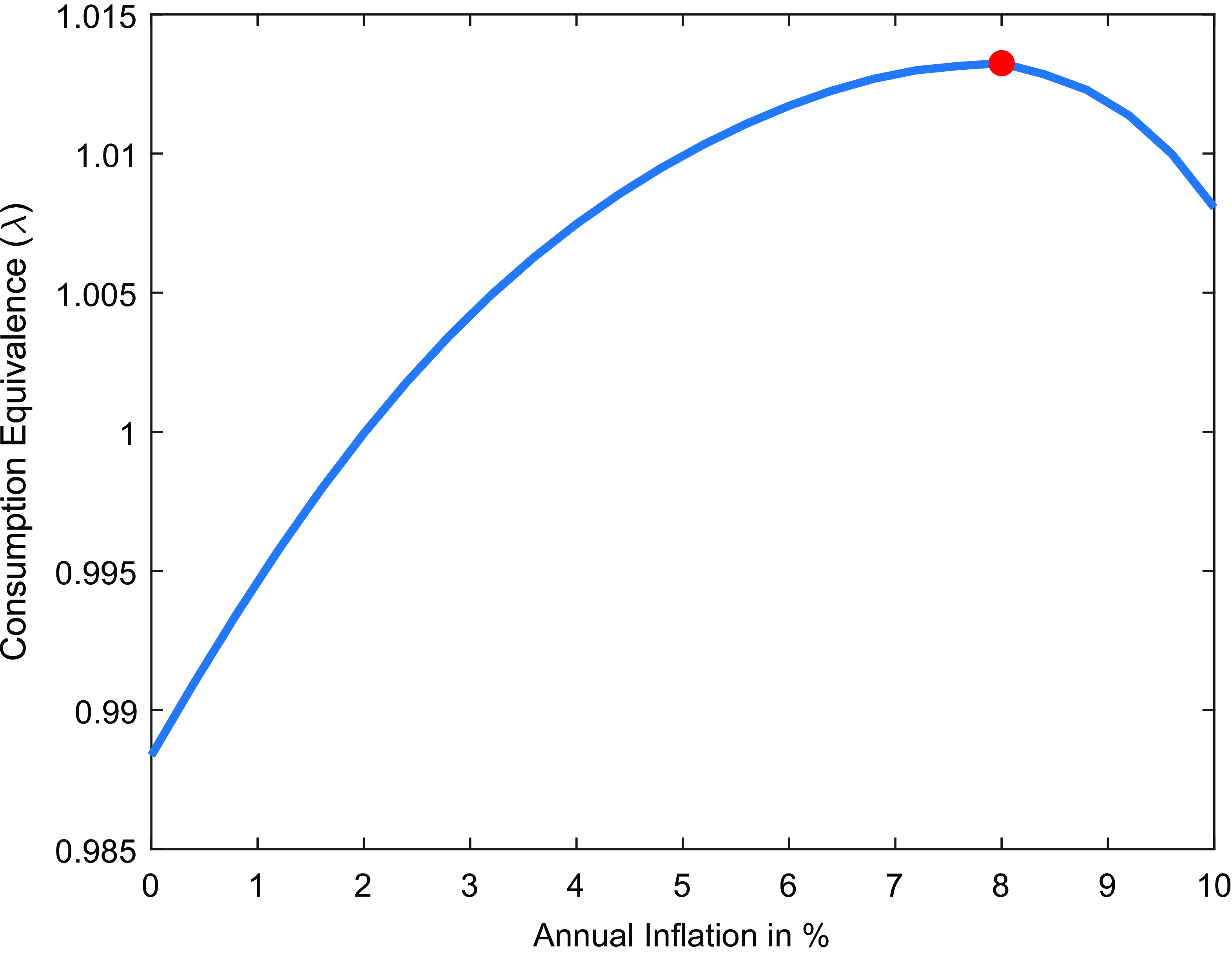
Figure B1. Welfare comparison.
Notes: The figure plots the consumption-equivalent welfare as a function of the steady-state inflation rate relative to welfare when the inflation target is 2 percent. There is a one-time unexpected demand shock to economies with different inflation targets and the long-run welfare in these economies are compared. Red circle indicates the peak of the curve. The welfare gain is around 1.4% when the inflation target is 8% compared to the benchmark economy with 2% target.
In addition to the DNWR channel, the high welfare cost of the ZLB also contributes to the increase in the optimal inflation rate from 7% to 8%. However, if the discount rate shock is small, the optimal inflation rate would be closer to the steady state rate of 7%, given the diminishing cost of ZLB.
The model presented in this study suggests that adjusting the inflation target to the optimal rate in the face of a negative aggregate shock leads to an improvement in welfare. These findings are in line with previous literature (Coibion et al. Reference Coibion, Gorodnichenko and Wieland2012), which suggests that in a representative agent setting, the DNWR constraint reduces the frequency of the ZLB by causing a smaller decline in the inflation rate in response to a negative demand shock. Therefore, the decrease in the frequency of binding ZLB reduces the benefit of higher inflation: lower inflation might be desirable because the DNWR constraint binds more and decreases the binding rate of the ZLB constraint. However, as demonstrated in the model,incorporating heterogeneity in idiosyncratic productivity and making the DNWR constraint binding at the household level results in a much higher welfare cost of DNWR, suggesting that a higher optimal inflation rate is necessary to mitigate the negative impact of the DNWR channel. In short, considering the price dispersion due to sticky prices, zero lower bound, and declining trend productivity, I find that the optimal inflation target should be much higher than 2%, close to 7%, to mitigate the negative effects of DNWR on the labor market and to increase long-run welfare.
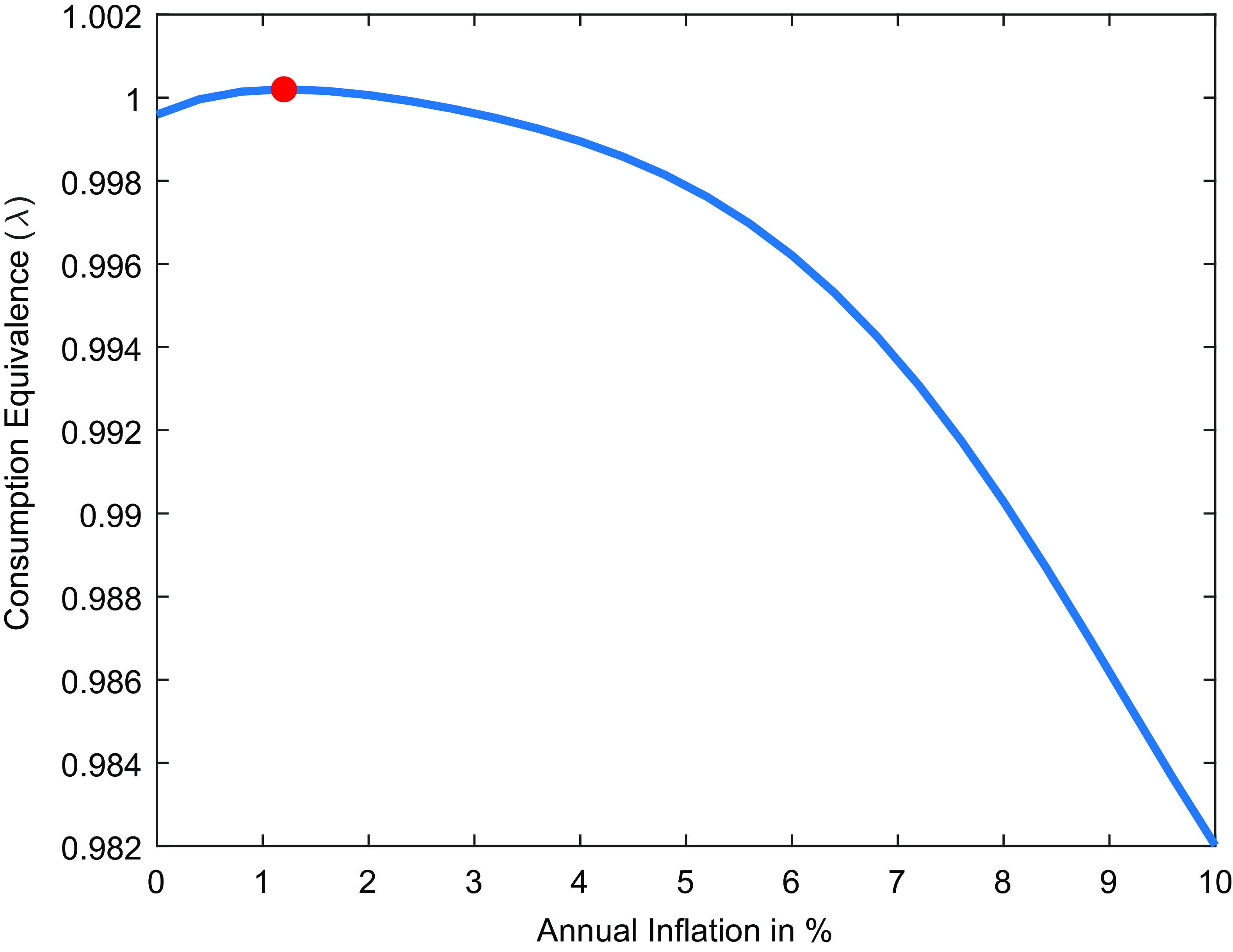
Figure B2. Welfare comparison, representative agent model.
Notes: The figure plots the consumption-equivalent welfare as a function of the steady-state inflation rate relative to welfare when the inflation target is 2 percent. There is a one-time unexpected demand shock to economies with different inflation targets and the long-run welfare in these economies are compared. Red circle indicates the peak of the curve.
A comparison with previous literature becomes clearer when the model is applied to a representative agent scenario, where there is no heterogeneity in idiosyncratic productivity (Figure-B2). The model is the same except for the fact that there is no heterogeneity in idiosyncratic productivity and thus it is a representative agent model. In this scenario, the optimal inflation rate is estimated to be around 1.2% due to the presence of the ZLB constraint. However, if there were no ZLB and DNWR, the optimal inflation rate in a representative agent economy would be 0% due to the prevalence of the sand effect.
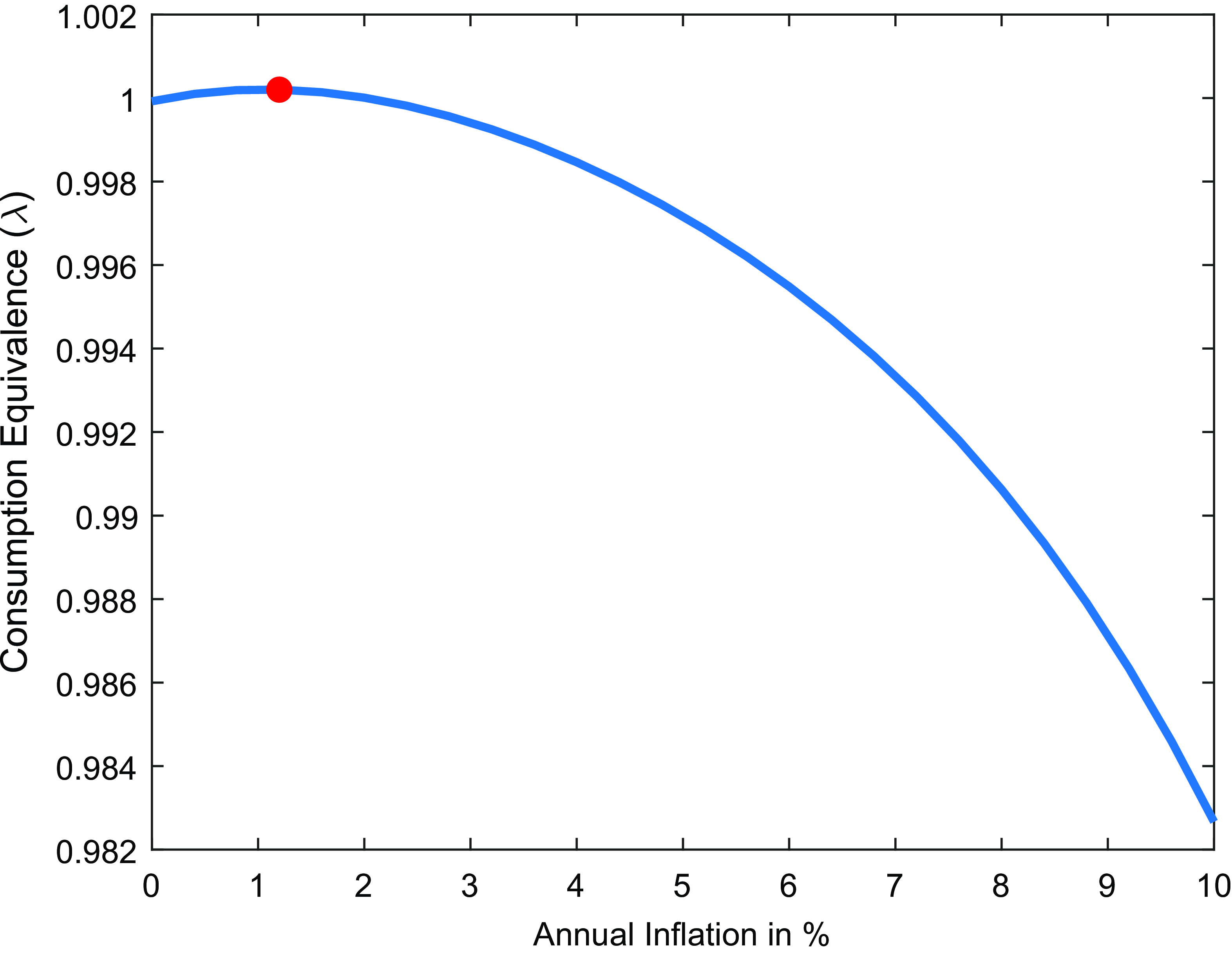
Figure B3. Welfare comparison, flexible wage.
Notes: The figure plots the consumption-equivalent welfare as a function of the steady-state inflation rate relative to welfare when the inflation target is 2 percent. There is a one-time unexpected demand shock to economies with different inflation targets and the long-run welfare in these economies are compared. Red circle indicates the peak of the curve.
As depicted in Figure-B3, when wages are fully flexible under a heterogeneous agent setting and there are only price stickiness and the ZLB constraint, the welfare cost is actually similar to the representative agent case. Since there is no inefficiency stemming from wages, the trade-off between inflation and ZLB determines the optimal inflation rate. A slightly higher inflation target, around 1.2% is optimal because ZLB is less likely to bind and this is consistent with what literature finds (Coibion et al. Reference Coibion, Gorodnichenko and Wieland2012).
Appendix - C - Extensions
Empirical wage change distribution
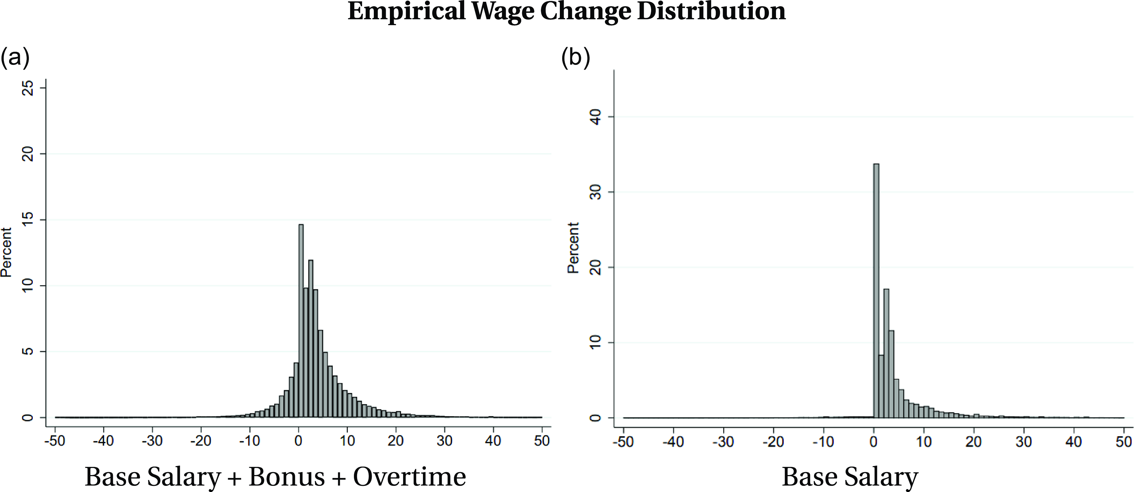
Figure C1. The % change in annual salary, Grigsby et al. (Reference Grigsby, Hurst and Yildirmaz2021).
The figure, sourced from Grigsby et al. (Reference Grigsby, Hurst and Yildirmaz2021), shows that even when additional payments are included, the spike at zero remains significant, and wage cuts are not uncommon. In this study, I analyze the welfare implications of wage freezes observed in the data by accurately matching the distributions, using a slight deviation from the standard New Keynesian model. One specification incorporates a low freeze rate, providing a lower bound for welfare cost estimates, while another adopts a high freeze rate, offering an upper bound for these estimates.
Correlation between inflation and wage freeze rate
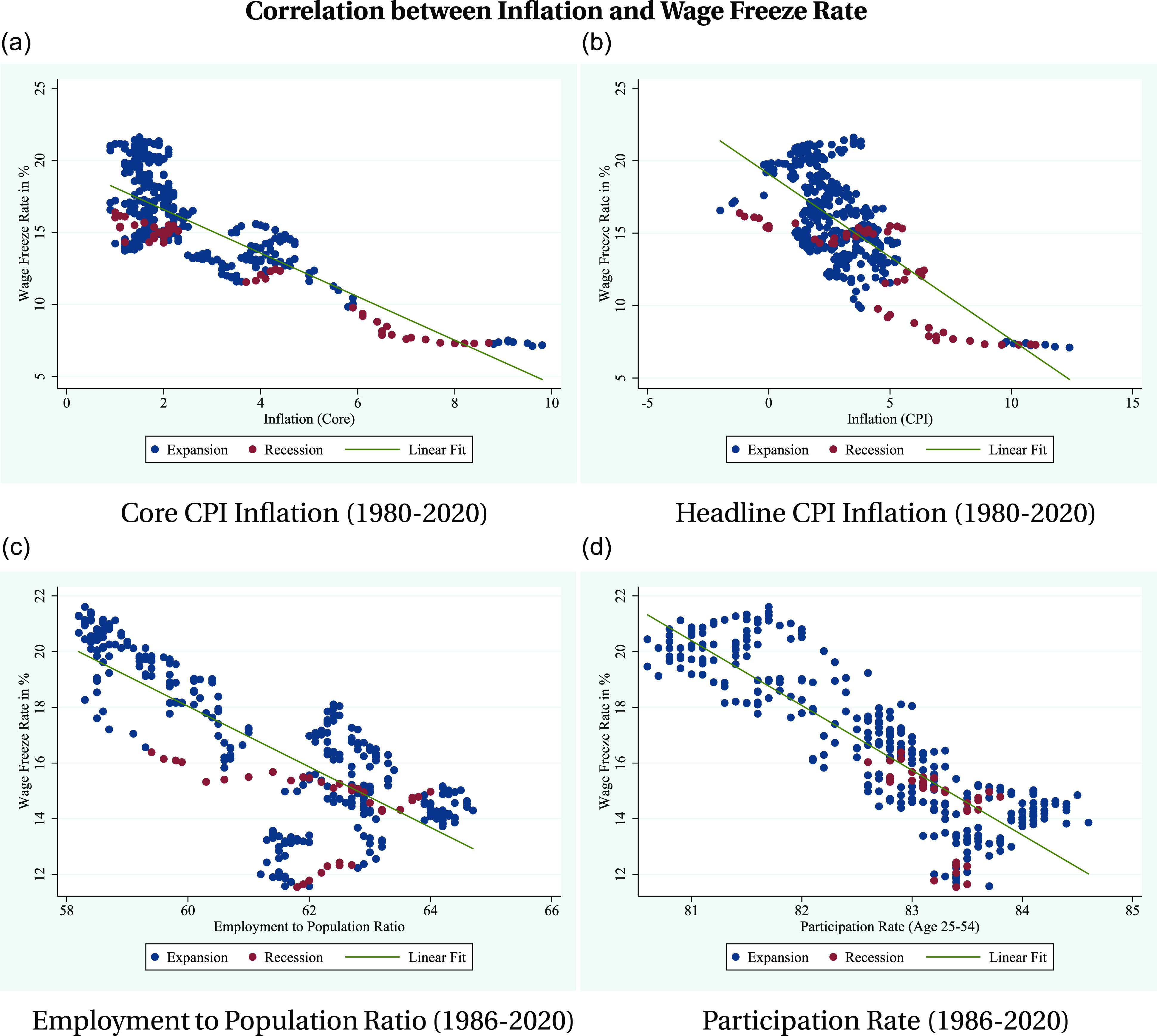
Figure C2. Correlation between inflation and wage freeze rate.
Notes: The figure depicts the correlation between wage freeze rates and inflation, as well as employment measures. Red dots represent periods of recession as identified by NBER-dated recessions.
Consistent with the theory, the correlation between the wage freeze rate and the inflation rate is negative and remains robust across different measures of inflation, as analyzed in detail by Jo (Reference Jo2021).
Other sensitivity analysis
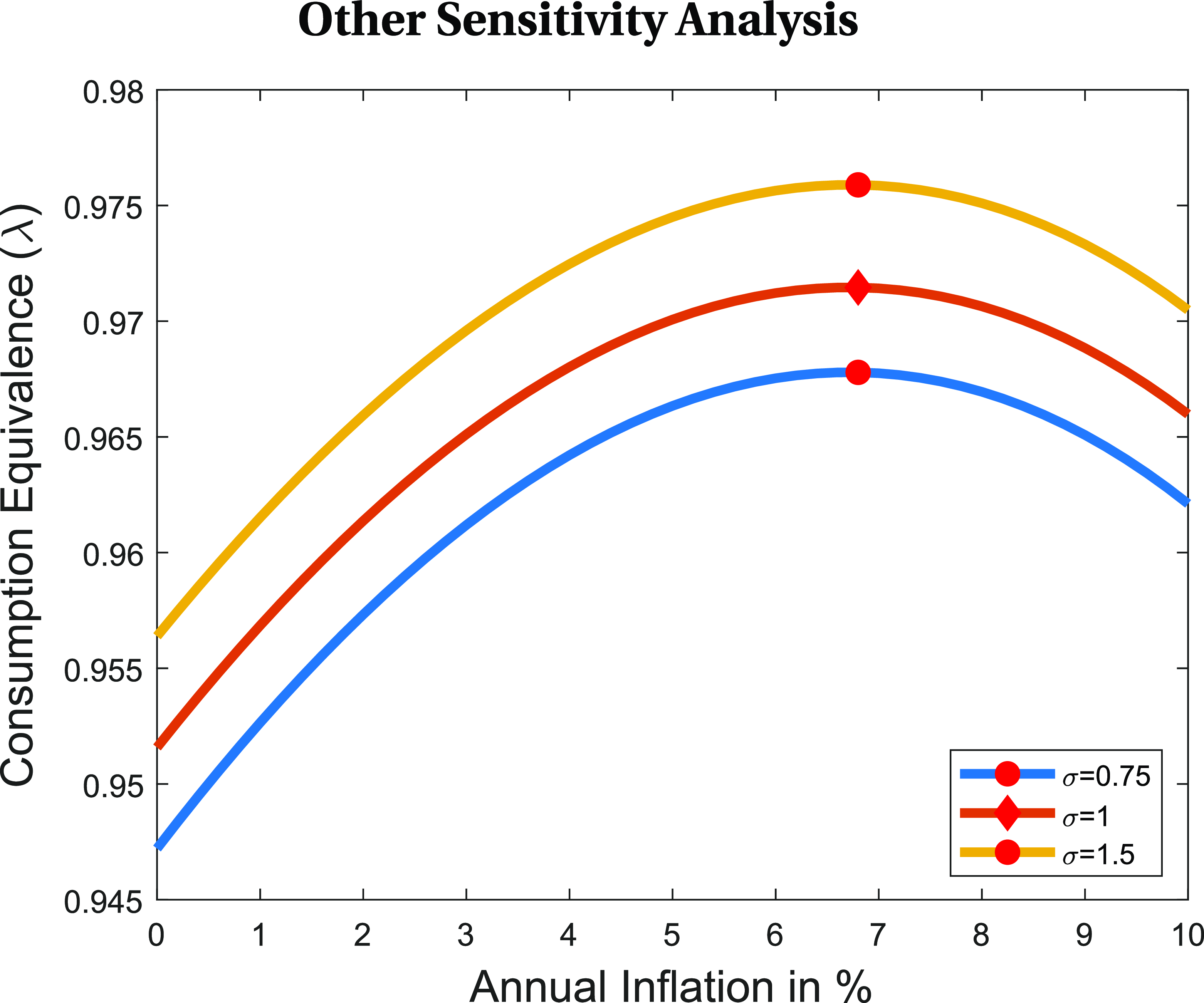
Figure C3. Optimal inflation rate, risk aversion.
Notes: The figure plots the consumption-equivalent welfare of economies with different risk aversion parameter as a function of the inflation rate relative to welfare when prices are completely flexible. Diamond shape indicates the benchmark case.
As Figure-C3 illustrates, the risk aversion parameter is not critical for the analysis due to the separable utility function. Adjusting $\sigma$
only produces a level effect, as consumption is fully insured across agents, and there is no heterogeneity in consumption levels. The key difference lies in the labor supply of households, which depends on their productivity level and the wage from the previous period.
$\sigma$
only produces a level effect, as consumption is fully insured across agents, and there is no heterogeneity in consumption levels. The key difference lies in the labor supply of households, which depends on their productivity level and the wage from the previous period.
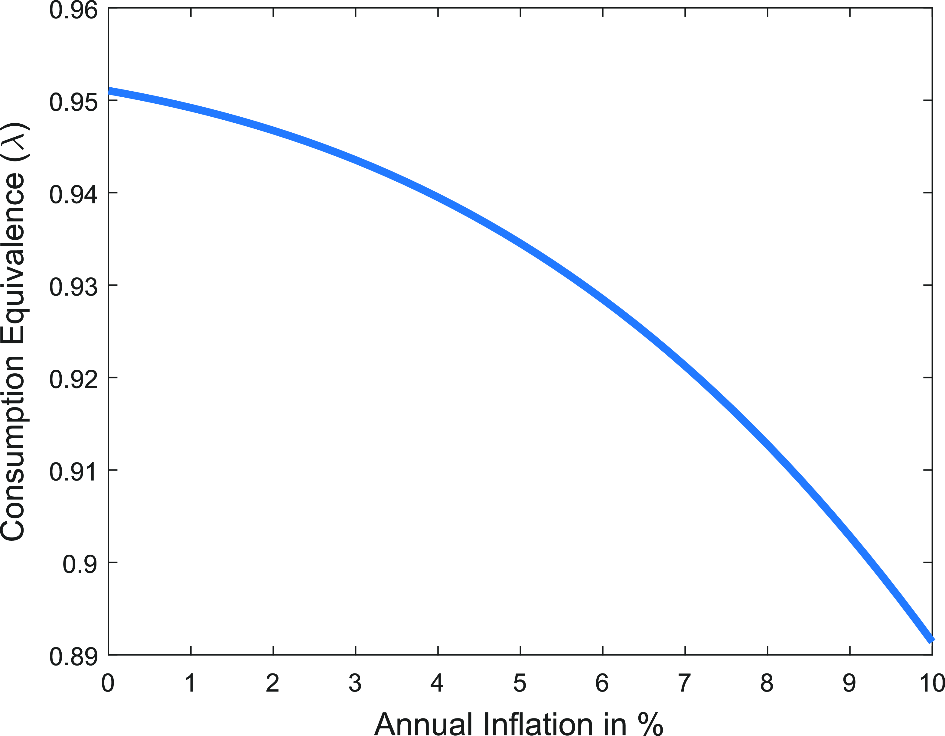
Figure C4. Optimal inflation rate, standard wage rigidity. The figure plots the consumption-equivalent welfare as a function of the inflation rate relative to welfare when prices are completely flexible. Here, instead of asymmetric wage rigidity, standard Calvo-type wage rigidity is assumed.
Instead of an asymmetry in wage contracts, if there are standard staggered wage contracts a la. Calvo (Reference Calvo1983), then there is no welfare gain from a higher inflation target. In contrast, there is a significant welfare cost. In this case, wages are rigid both downward and upward for a fraction of households each period, and constrained households cannot adjust their wages freely upon receiving idiosyncratic productivity shocks. When there is positive inflation, households would want to adjust their wages even in the absence of shocks. As depicted in Figure-C4, as inflation gets higher, the welfare cost is higher under standard staggered wage contracts. However, in my model, households can flexibly adjust wages upward and only a fraction cannot adjust downward, which creates the freeze rate in the economy. So, a positive inflation target helps because households are less likely to decrease and more likely to increase wages. Since they can flexibly increase wages, the welfare cost is much less with a higher inflation target.
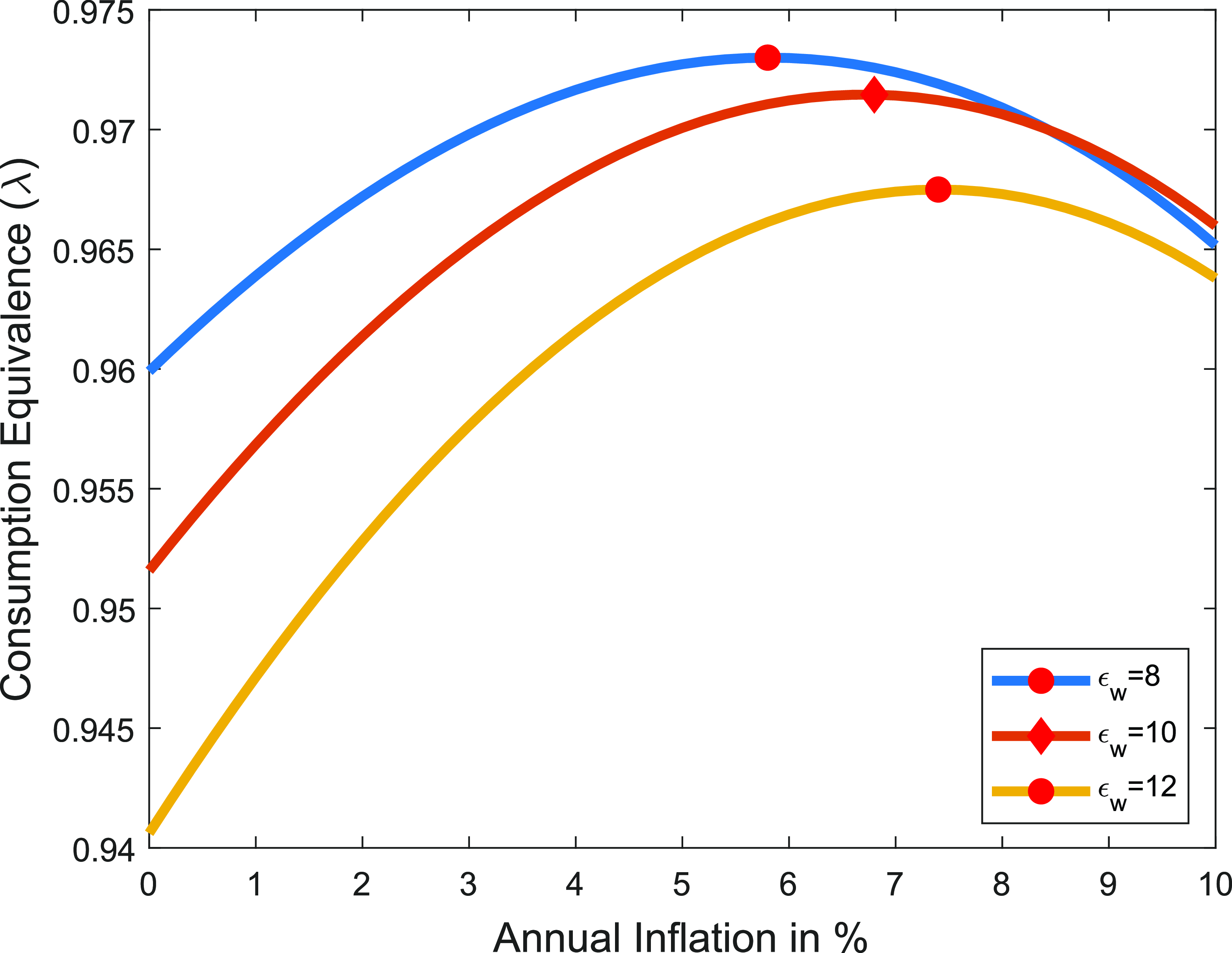
Figure C5. Optimal inflation rate, elasticity $\epsilon _{w}$
. The figure plots the consumption-equivalent welfare of economies with different
$\epsilon _{w}$
. The figure plots the consumption-equivalent welfare of economies with different $\epsilon _w$
values as a function of the inflation rate relative to welfare when prices are completely flexible. Diamond shape indicates the benchmark case.
$\epsilon _w$
values as a function of the inflation rate relative to welfare when prices are completely flexible. Diamond shape indicates the benchmark case.
Since the elasticity parameter $\epsilon _w$
directly impacts the wage setting mechanism, I check the robustness of results with respect to it. Figure-C5 indicates that the optimal inflation rate is still higher than 5 percent even for a low level of wage elasticity. Being analogous to price stickiness, the welfare cost of wage stickiness is higher with higher elasticity of substitution. As a result, as
$\epsilon _w$
directly impacts the wage setting mechanism, I check the robustness of results with respect to it. Figure-C5 indicates that the optimal inflation rate is still higher than 5 percent even for a low level of wage elasticity. Being analogous to price stickiness, the welfare cost of wage stickiness is higher with higher elasticity of substitution. As a result, as $\epsilon _{w}$
gets higher, the distortionary impact of the DNWR channel is higher and thus the optimal inflation rate is higher compared to the benchmark case.Footnote
45
$\epsilon _{w}$
gets higher, the distortionary impact of the DNWR channel is higher and thus the optimal inflation rate is higher compared to the benchmark case.Footnote
45
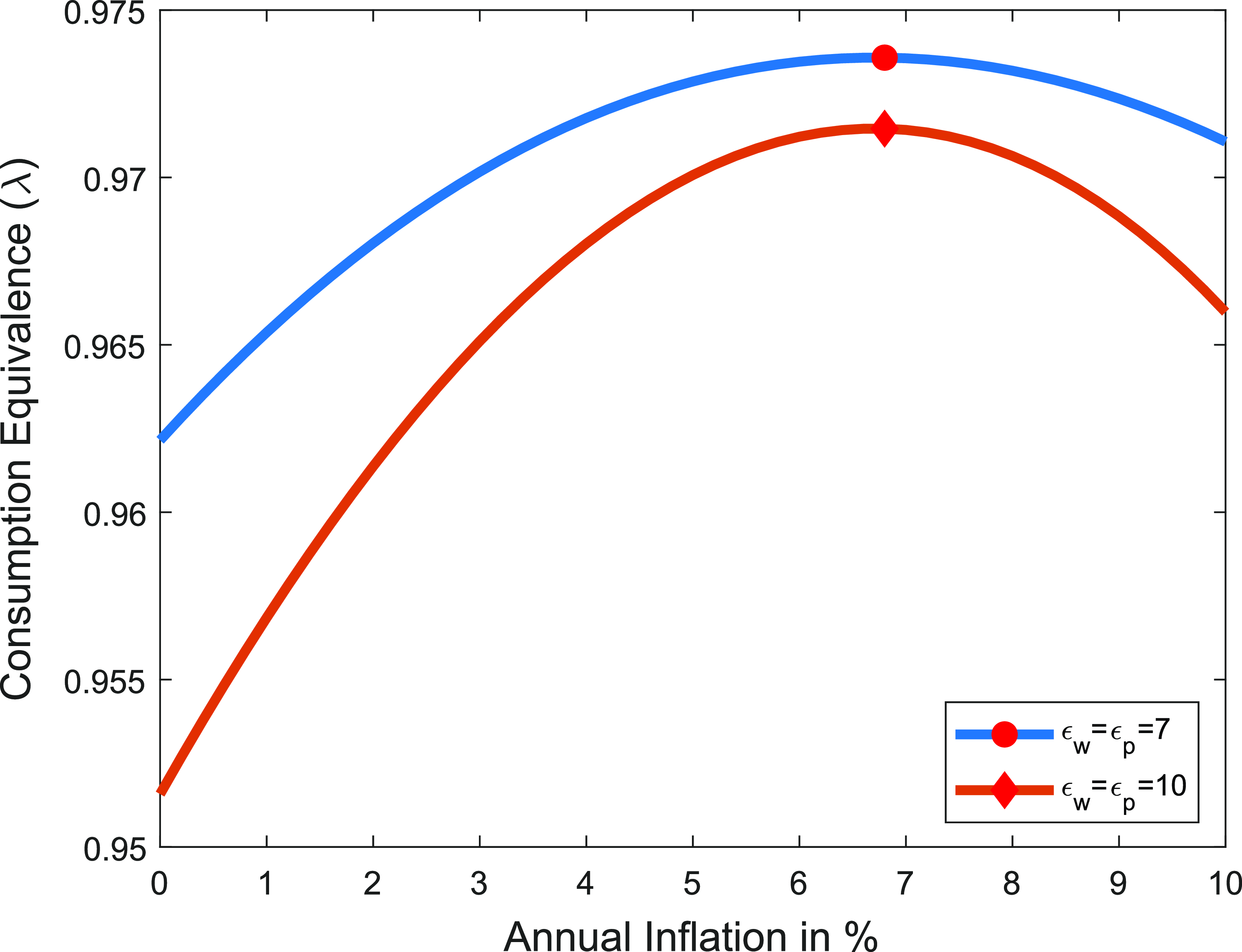
Figure C6. Optimal inflation rate, elasticity of substitution. The figure plots the consumption-equivalent welfare of economies with different elasticity $\epsilon _w=\epsilon _p$
values as a function of the inflation rate relative to welfare when prices are completely flexible. Diamond shape indicates the benchmark case.
$\epsilon _w=\epsilon _p$
values as a function of the inflation rate relative to welfare when prices are completely flexible. Diamond shape indicates the benchmark case.
I also change elasticity of substitution to $\epsilon _{p}=\epsilon _{w}=7$
instead of 10Footnote
46
to see if it creates any changes on the optimal inflation rate, since a higher elasticity increases the strength of both channels in the trade-off. Figure-C6 shows that the optimal inflation target does not change; there is only a level effect. The reason is that the welfare cost of price stickiness is higher with a higher elasticity of substitution between intermediate goods (lower markup), as demand is more elastic to price changes, increasing goods market misallocations due to price rigidity. At the same time, the welfare cost of DNWR is higher with a more elastic labor demand, as shown in Figure-C5. Higher elasticities (
$\epsilon _{p}=\epsilon _{w}=7$
instead of 10Footnote
46
to see if it creates any changes on the optimal inflation rate, since a higher elasticity increases the strength of both channels in the trade-off. Figure-C6 shows that the optimal inflation target does not change; there is only a level effect. The reason is that the welfare cost of price stickiness is higher with a higher elasticity of substitution between intermediate goods (lower markup), as demand is more elastic to price changes, increasing goods market misallocations due to price rigidity. At the same time, the welfare cost of DNWR is higher with a more elastic labor demand, as shown in Figure-C5. Higher elasticities ( $\epsilon _p$
and
$\epsilon _p$
and $\epsilon _w$
) lead to an increase in the welfare cost of both the price dispersion channel and the DNWR channel. These effects cancel each other out in terms of shifting the optimal rate, but we observe a significant level effect.
$\epsilon _w$
) lead to an increase in the welfare cost of both the price dispersion channel and the DNWR channel. These effects cancel each other out in terms of shifting the optimal rate, but we observe a significant level effect.
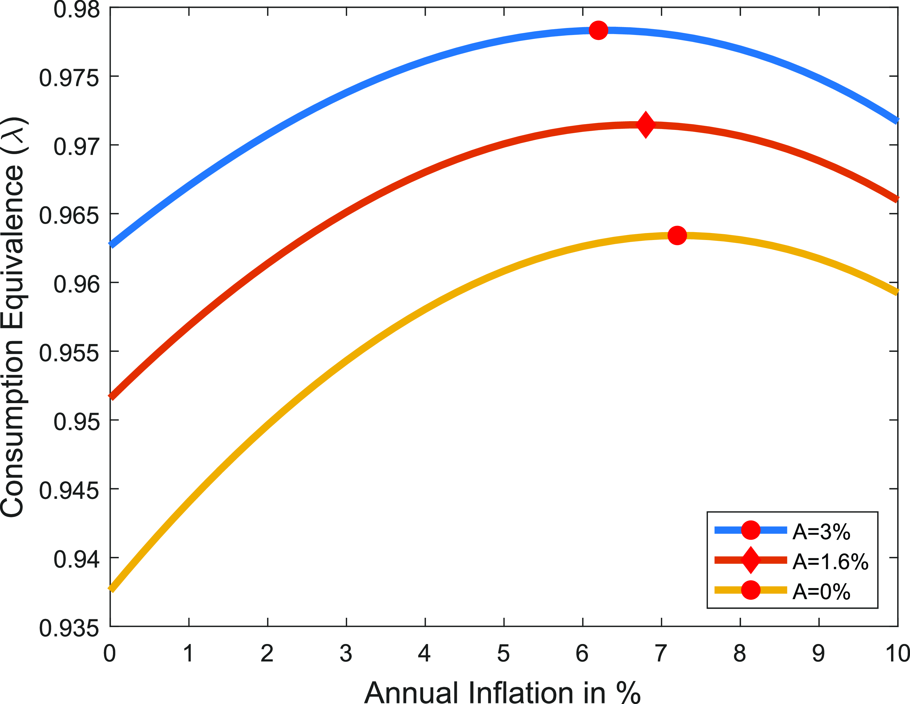
Figure C7. Optimal inflation rate, trend productivity growth. The figure plots the consumption-equivalent welfare of economies with different trend productivity growth as a function of the inflation rate relative to welfare when prices are completely flexible. Diamond shape indicates the benchmark case.
Figure-C7 shows that higher trend productivity growth makes the DNWR constraint less binding, resulting in a lower welfare cost from this channel. Consequently, the optimal inflation rate is higher when trend productivity growth is lower. Data indicates that trend productivity growth has been declining over the last few decades, and if this trend continues, the DNWR constraint will become even costlier. As a result, the optimal inflation rate should be even higher compared to the benchmark case, exceeding 7%.
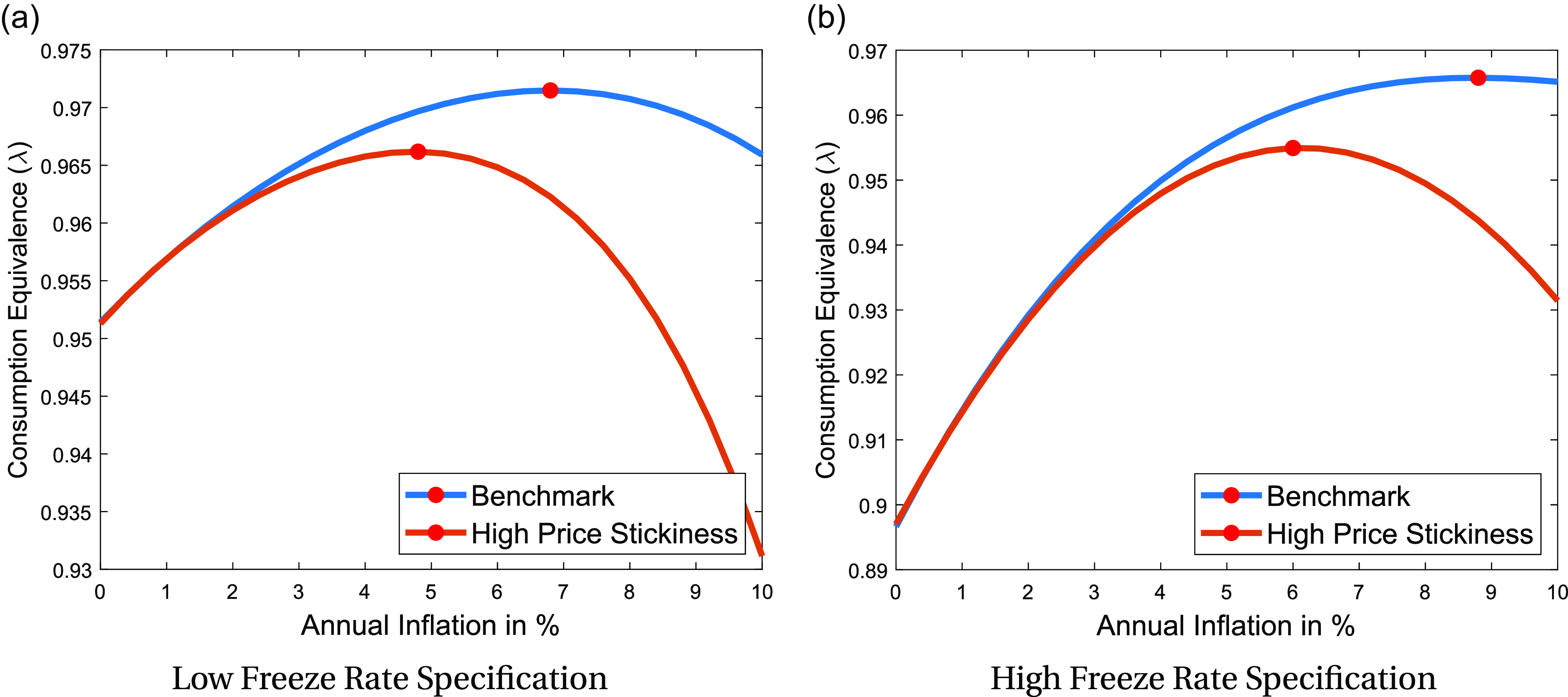
Figure C8. Welfare cost of DNWR and sticky prices (High price stickiness).
Notes: The figure plots the consumption-equivalent welfare as a function of the inflation rate, relative to welfare under completely flexible prices. It compares two cases: one where the duration of price rigidity is 7 months (benchmark) and one with 9 months (high stickiness). Panel (a) presents the results for the specification where the annual total wage change distribution is matched, while Panel (b) shows the results for the specification where the annual base wage change distribution is matched. The figure quantifies the trade-off between these channels and indicates that the optimal inflation target is 4.8% for the low freeze rate case and 6.0% for the high freeze rate when the duration of price rigidity is assumed to be 9 months instead of 7 months.
To examine how the optimal rate changes with price stickiness, I conduct an additional robustness check by increasing the frequency of price changes from 7 months to 9 months and replicating the analysis in Figure-3. In Figure-C8, the results show that the optimal rate for the low freeze rate specification decreases from 6.8% to 4.8%, and for the high freeze rate specification, it decreases from 8.8% to 6.0%. This is because price dispersion increases and price stickiness becomes more costly.
Beyond the zero lower bound and downward nominal wage rigidity, there can be other channels that can affect the optimal inflation rate as discussed in Schmitt-Grohe and Uribe (Reference Schmitt-Grohe and Uribe2016). One is the existence of tax evasion or an underground (informal) economy, which cannot be taxed directly. Therefore, a positive inflation rate might help to tax this sector indirectly. However, they state that the empirical estimates show that the size of the informal sector in the U.S. is at most 10% so that one should not worry much about that issue in the context of the U.S. Another channel can be the demand for money. Money balances provide transaction services to households and the cost of printing money is zero. Therefore, it is optimal to set the opportunity cost of holding money as low as possible. Thus, optimal inflation should be low as well. In this paper, I did not incorporate this feature into my model.
In the absence of lump-sum taxes, inflation acts as an implicit tax, making a positive inflation rate optimal (Phelps, Reference Phelps1973). Higher inflation, however, may increase markups and risks, reducing the optimal rate (King and Wolman, Reference King and Wolman1996; Ascari and Sbordone, Reference Ascari and Sbordone2014; Di Tella et al. Reference Di Tella, Malgieri and Tonetti2024). Similarly, higher inflation may destabilize expectations and amplify volatility, pushing the optimal rate lower (Ascari and Sbordone, Reference Ascari and Sbordone2014). On the other hand, price flexibility increases with higher inflation, potentially raising the optimal rate (Nakamura et al. Reference Nakamura, Steinsson, Sun and Villar2018).

Figure C9. Welfare cost of DNWR, no persistence in shock.
Notes: The figure plots the wage change distribution at different frequencies. The model is run quarterly and the distribution is then annualized to match the empirical one. The persistence of the productivity process is set to zero, and the standard deviation of wage changes is matched to the standard deviation of the stochastic process.

Figure C10. Quarterly distribution of wage changes under DNWR at 2% trend inflation.
Notes: The figure plots the quarterly wage change distribution for two specifications considered in the paper. The first specification includes total wage changes and has a lower freeze rate, while the second specification includes base wage changes and has a higher freeze rate. The wage freeze rate, mean and standard deviation of wage changes are targeted moments.
Structural shifts, such as a declining natural rate of interest, also necessitate a higher optimal inflation target (Andrade et al. Reference Andrade, Gali, Bihan and Matheron2019). Behavioral channels, such as rational inattention, suggest that inflation might encourage more attentive agents, supporting a higher rate. Similarly, the Balassa-Samuelson effect implies a higher optimal rate for developing economies with productivity gaps in tradable versus non-tradable sectors. Labor market frictions, such as search costs, also favor a slightly higher inflation rate to improve market flexibility (Carlsson and Westermark, Reference Carlsson and Westermark2016). In contrast, mismeasurement of CPI inflation due to methodological biases may necessitate a lower inflation target to account for overstated inflation.
Other channels include financial frictions and limited participation in asset markets (Brunnermeier and Sannikov, Reference Brunnermeier and Sannikov2016), which could justify higher inflation to ease financial constraints, and the role of the informal sector, where inflation serves as an implicit tax on cash-intensive activities, particularly in economies with significant underground economies or foreign-held currency balances. While these factors provide a nuanced perspective, the empirical relevance of each channel depends on the economic context, as highlighted in Schmitt-Grohe and Uribe (Reference Schmitt-Grohe and Uribe2016). See Adam et al. (Reference Adam, Weber and Submitter2024) for a detailed review of the literature.
In Figure-C9, I examine the implications of the persistence of labor productivity shocks. The persistence of the productivity process is set to zero, and the standard deviation of wage changes is matched to the standard deviation of the stochastic process. Compared to the benchmark case presented in Figure-1, the wage freeze rate is slightly lower, and there are more wage cuts. However, the welfare cost remains significant and follows a similar pattern, resulting in a comparable optimal inflation rate. Instead of assuming no persistence, I use the persistence parameter estimated by Guvenen (Reference Guvenen2009), which, depending on the specification, can result in a wage freeze rate as high as 33%.
Lastly, in Figure-C10, similar to Figure-1, I present the quarterly versions of the distributions for both specifications used in the paper.


 Open access