Multivariate functorial difference

Abstract

Partial difference operators for a large class of functors between presheaf categories are introduced, extending our previous work on the difference operator to the multivariable case. These combine into the Jacobian profunctor that provides the setting for a lax chain rule. We introduce a functorial version of multivariable Newton series whose aim is to recover a functor from its iterated differences. Not all functors are recovered; however, we get a best approximation in the form of a left adjoint, and the induced comonad is idempotent. Its fixed points are what we call soft analytic functors, a generalization of the well-studied multivariable analytic functors.

In memory of Phil Scott, 1947–2023

Philip Scott

I knew Phil for most of his career, from when he was a post-doctoral fellow at McGill in 1977, a colleague the following year at Dalhousie, and a friend ever since. His knowledge of the literature in category theory, logic, and computer science was phenomenal. He traveled a lot and spoke to many people. This way, he kept up to date on the latest developments, and each time he visited Halifax, he had some new topic he thought I should look at. This was good advice, which I wish I had been more diligent following up. We have lost a great ambassador for our subject as well as a friend. I dedicate this work to him.

Introduction

This is a sequel to Paré (2024). Here, we are interested in the structure of functors $ \textbf {Set}^{\textbf {A}} \longrightarrow \textbf {Set}^{\textbf {B}}$ ( $\textbf {A}$ and $\textbf {B}$ small categories) generalizing the difference calculus for endofunctors of $ \textbf {Set}$ . An important example is given by the generalized analytic functors of Fiore et al. (2008). As in that work, profunctors are central. That is perhaps the main difference the present work has with Paré (2024). This is somewhat of a simplification like saying that multivariate calculus is just single variable calculus plus linear algebra. The added dimensions open up a whole array of possibilities.

The work here is a categorified version of the classical partial difference operators for real functions

\begin{equation*} {\mathbb R}^n \longrightarrow {\mathbb R}^m \rlap {\,,} \end{equation*}

a discrete version of partial derivatives. The analogy is quite fruitful.

As the paper is quite long, it may be helpful to point out the main results, namely the lax chain rule (Theorem4.2) and the Newton adjunction (Theorem5.1) together with the convergence theorem (Theorem5.2). These results are proper to the categorical setting and have no counterpart for real-valued functions. They could not be formulated without the pivotal definitions of the (discrete) Jacobian as a profunctor (Definition4.1) and soft analytic functor (Definition5.2).

Apart from the obvious (Fiore et al. 2008) and the references therein, the present work was strongly influenced by the work of the Calgary-Ottawa-Montreal consortium on tangent categories and Cartesian differential categories. Several talks in the ATCAT seminar by regulars Geoff Cruttwell and Marcello Lanfranchi as well as guest speakers, notably Robin Cockett and JS Lemay, helped form my ideas on the categorical theory of differentials. After completion of this work, the paper “Cartesian difference categories” by Alvarez-Picallo and Pacaud Lemay (2021) came to my attention. This is clearly relevant as it deals with the categorical understanding of finite difference. What is less clear is precisely how they are related. Further work in this direction should prove fruitful.

Thanks to Nathanael Arkor, Andreas Blass, John Bourke, Aaron Fairbanks, Marcelo Fiore, Richard Garner, Theo Johnson-Freyd, Tom Leinster, Matías Menni, Deni Salja, and Peter Selinger for their insightful comments and interest. A special thanks to Peter Selinger for helping me prepare the final version in the MSC style.

1. Profunctors

Profunctors (a.k.a. bimodules, modules, and distributors) will be at the heart of this work. Widely viewed as categorified relations, for our purposes, they are better viewed as categorified matrices. They correspond to cocontinuous functors between functor categories. Such functors are considered to be linear. This section contains nothing new (except perhaps Definition1.2 and Proposition1.2). It is included for completeness and to set notation.

1.1 Definitions

We have opted, not without thought, for the following definition, which is the opposite of the majority view.

Definition 1.1. (Lawvere, Bénabou) Let $ \textbf {A}$ and $ \textbf {B}$ be small categories. A profunctor is a functor $ P \colon \textbf {A}^{op} \times \textbf {B} \longrightarrow \textbf {Set}$ . A morphism of profunctors $ t \colon P \longrightarrow Q$ is a natural transformation.

This gives the basic data for a bicategory, $ {\mathscr{P}}{\kern.5pt}\textit {rof}$ , of profunctors. Composition is given by “matrix multiplication,” which takes the form of a coend. For and , the composite $ Q \otimes P$ is defined by

\begin{equation*} Q \otimes P (A, C) = \int ^{B \in \textbf {B}} Q (B, C) \times P (A, B) \rlap {\,.} \end{equation*}

The identity is the hom functor

\begin{equation*} {\textrm {Id}}_{\textbf {A}} (A, A') = \textbf {A} (A, A') \rlap {\,.} \end{equation*}

The reader is referred to the standard texts (see, e.g., Borceaux (1994b)) for a proof that we do get a bicategory.

For explicit computations involving profunctors, the following notation is useful. An element $ x \in P (A, B)$ is denoted by a pointed arrow, sometimes called a heteromorphism, if it’s necessary to keep track of the profunctor. The functoriality of $ P$ manifests itself as a composition

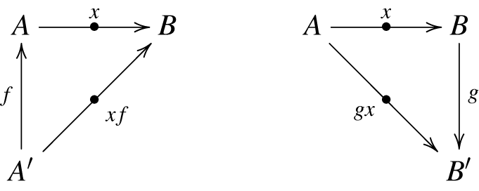
which is associative (left, right, and middle) and unitary.

It is in dealing with composition that this is most useful. An element of $ Q \otimes P (A, C)$ is an equivalence class of pairs

where the equivalence relation is generated by identifying and if we have

so they are equivalent iff there exists a path of pairs

We write the equivalence class as

\begin{equation*} y \otimes _B x \ \ \mbox{or simply} \ \ y \otimes x \rlap {\,.} \end{equation*}

The equivalence relation is generated by

\begin{equation*} y b \otimes x = y \otimes b x \rlap {\,.} \end{equation*}

Every functor $ F \colon \textbf {A} \longrightarrow \textbf {B}$ induces two profunctors

and

\begin{equation*}F_* (A, B) = \textbf {B} (FA, B) \quad \quad F^* (B, A) = \textbf {B} (B, FA) . \end{equation*}

$ F^*$ is right adjoint to $ F_*$ in $ {\mathscr{P}}{\kern.5pt}\textit {rof}$ .

1.2 Biclosedness

The bicategory $ {\mathscr{P}}{\kern.5pt}\textit {rof}$ is biclosed, that is, $ \otimes$ admits right adjoints in each variable giving two hom profunctors $ \oslash$ and characterized by natural bijections

for profunctors

We use Lambek’s notation for the internal homs. Inasmuch as $ \otimes$ is a product, the right adjoints are quotients of a sort.

An element of $ (Q\ \varnothing_{C}\ R) (A, B)$ is a $ \textbf {C}$ -natural transformation

\begin{equation*} t \colon Q (B, -) \longrightarrow R (A, -) \end{equation*}

and an element of $(R$ $_{\textbf {A}}\, P) (B, C)$ is an $ \textbf {A}$ -natural transformation

\begin{equation*} u \colon P (-, B) \longrightarrow R (-, C)\rlap {\,.} \end{equation*}

1.3 Cocontinuous functors

Our interest is in functors between functor categories and a profunctor will produce an adjoint pair of them. A profunctor: is a functor

\begin{equation*} \textbf {1}^{op} \times \textbf {A} \longrightarrow \textbf {Set} \end{equation*}

which we identify with a functor $ \Phi \colon \textbf {A} \longrightarrow \textbf {Set}$ . A profunctor will then produce, by composition, a functor

\begin{equation*} P \otimes _{\textbf {A}} (\ \ ) \colon \textbf {Set}^{\textbf {A}} \longrightarrow \textbf {Set}^{\textbf {B}} \end{equation*}

with a right adjoint

It follows that $ P \otimes _{\textbf {A}} (\ \ )$ is cocontinuous and is considered to be the linear functor corresponding to the matrix $ P$ .

As is well known, we have

Proposition 1.1. The following categories are equivalent:

1. (1) Profunctors

2. (2) Cocontinuous functors $ \textbf {Set}^{\textbf {A}} \longrightarrow \textbf {Set}^{\textbf {B}}$

3. (3) Adjoint pairs

Given a cocontinuous functor $ F \colon \textbf {Set}^{\textbf {A}} \longrightarrow \textbf {Set}^{\textbf {B}}$ , the corresponding profunctor is given by

\begin{equation*} P (A, B) = F (\textbf {A} (A, -)) (B) \rlap {\,.} \end{equation*}

Note that this doesn’t use cocontinuity of $ F$ , which leads to the following.

Definition 1.2. The core of a functor $ F \colon \textbf {Set}^{\textbf {A}} \longrightarrow \textbf {Set}^{\textbf {B}}$ is the profunctor defined by

\begin{equation*} \mbox{Cor} (F) (A, B) = F (\textbf {A} (A, -)) (B) \rlap {\,.} \end{equation*}

The functor

\begin{equation*} \mbox{Cor} (F) \otimes (\ \ ) \colon \textbf {Set}^{\textbf {A}} \longrightarrow \textbf {Set}^{\textbf {B}} \end{equation*}

is the “linear core” of $ F$ .

Proposition 1.2. $ Cor $ is right adjoint to the functor $ {\mathscr{P}}{\kern.5pt}\textit {rof} (\textbf {A}, \textbf {B}) \longrightarrow {{\mathscr{C}}{\kern.5pt}\textit {at}} (\textbf {Set}^{\textbf {A}}, \textbf {Set}^{\textbf {B}})$ which takes a profunctor $ P$ to the (cocontinuous) functor $ P \otimes _{\textbf {A}} (\ \ )$ .

Proof. A profunctor can be viewed, by exponential adjointness, as a functor $ \textbf {A}^{op} \longrightarrow \textbf {Set}^{\textbf {B}}$ . Then, $ \mbox{Cor}$ is just restriction along the Yoneda embedding

\begin{equation*} F \colon \textbf {Set}^{\textbf {A}} \longrightarrow \textbf {Set}^{\textbf {B}}\quad \longmapsto \quad \textbf {A}^{op} \longrightarrow^Y \textbf {Set}^{\textbf {A}} \longrightarrow^F \textbf {Set}^{\textbf {B}} \end{equation*}

and $ P \otimes _{\textbf {A}} (\ \ )$ is left Kan extension

Thus for $ F \colon \textbf {Set}^{\textbf {A}} \longrightarrow \textbf {Set}^{\textbf {B}}$ , $ \mbox{Cor} (F) \otimes _A (\ \ )$ is the best approximation to $ F$ by a cocontinuous functor. As a matter of interest, the counit of the adjunction

\begin{equation*} \epsilon (F) \colon \mbox{Cor} (F) \otimes (\ \ ) \longrightarrow F \end{equation*}

is given as follows. An element of $ (\mbox{Cor} (F) \otimes \Phi )( B)$ is an equivalence class

so

\begin{equation*} [\textbf {A} (A, -) \xrightarrow{\hspace{6pt}{\bar {x}}\hspace{6pt}} \Phi , \ y \in F (\textbf {A} (A, -))(B)] \end{equation*}

giving

\begin{equation*} F (\textbf {A} (A, -))(B) \xrightarrow{F({\bar {x}})(B)} F (\Phi ) (B) \end{equation*}

\begin{equation*} y \longmapsto F ({\bar {x}})(B) (y) \rlap {\,.} \end{equation*}

Example 1.1. If $ \textbf {A}$ and $ \textbf {B}$ are discrete categories, i.e., sets $ A$ and $ B$ , then a profunctor is just a $ A \times B$ -matrix of sets $ [P_{ab}]$ and a morphism of profunctors $ P \longrightarrow P'$ a $ A \times B$ -matrix of functions. The identity $ {\textrm {Id}}_{\textbf {A}}$ is the matrix with $ 1$ ’s on the diagonal and $ 0$ elsewhere. If $ \textbf {C}$ is another discrete category and a profunctor, then $ Q \otimes _{\textbf {B}} P$ is the $ B \times C$ -matrix

\begin{equation*} \Bigg[ \sum _{b \in B} Q_{bc} \times P_{ab} \Bigg]_{\rlap {\,.}} \end{equation*}

If then

\begin{equation*} R \oslash _{\textbf {A}} P = \Bigg[\prod _{a \in A} R_{ac}^{P_{ab}} \Bigg] \end{equation*}

and

A profunctor is a $ 1 \times A$ matrix of sets, i.e., a vector $[X_a]$ and $ P \otimes _{\textbf {A}} X$ is the vector

\begin{equation*} \Bigg[ \sum _{a \in A} P_{ab} \times X_a\Bigg]_{b \rlap {\,.}} \end{equation*}

On the other hand for a $ B$ -vector,

\begin{equation*} \Bigg[\prod _b Y_b^{P_{ab}} \Bigg]_{a\rlap {\,.}} \end{equation*}

So, $ P \otimes _{\textbf {A}} (\ \ )$ is a “linear” functor and a “monomial” functor.

2. Tense Functors

In Paré (2024), we developed a difference calculus for taut endofunctors of $ \textbf {Set}$ , functors preserving inverse images. However, the important example of multivariable analytic functors of Fiore et al. (2008) is not taut. In fact, the linear functors $ P \otimes (\ \ )$ are not taut. They don’t even preserve monos. What we need are functors preserving complemented subobjects and their inverse images. Of course, in $ \textbf {Set}$ , all subobjects are complemented so it would make no difference, so maybe that’s what taut should be after all. But the word “taut” is pretty well established, so we use “tense” instead.

2.1 Complemented subobjects

In this section, we collect some useful facts about complemented subobjects in functor categories $ \textbf {Set}^{\textbf {A}}$ , most of which are well known from topos theory. We first list some general topos theory results, which will be useful for us. Proofs can be found in any of the standard topos theory books (see Borceaux (1994a) for an easily accessible account).

Definition 2.1. A subobject $ \Psi \, \succ\!\xrightarrow{\hspace{.3cm}} \, \Phi$ is complemented if there exists another subobject $ \Psi ' \succ\!\xrightarrow{\hspace{.3cm}} \Phi$ for which the induced morphishm $ \Psi + \Psi ' \longrightarrow \Phi$ is invertible.

We will use the hooked arrow as a reminder that $ \Psi$ is complemented,

Recall that every subobject $ \Psi \, \succ\!\xrightarrow{\hspace{.3cm}} \, \Phi$ has a pseudo-complement $ \neg \Psi \, \succ\!\xrightarrow{\hspace{.3cm}} \, \Phi$ , the largest subobject of $ \Phi$ whose intersection with $ \Psi$ is $ 0$ . It can be calculated as the pullback of the element $ \mbox{false} \colon 1 \, \succ\!\xrightarrow{\hspace{.3cm}} \, \Omega$ along the characteristic morphism of $ \Psi$ .

Proposition 2.1. 1. A subobject $ \Psi \, \succ\!\xrightarrow{\hspace{.3cm}} \, \Phi$ is complemented iff its characteristic morphism factors through $ 1 + 1$

2. Complemented subobjects are closed under composition.

3. Complemented objects are stable under pullback: if is complemented and $ f \colon \Theta \longrightarrow \Phi$ , then $ \neg f^{-1} (\Psi ) = f^{-1} (\neg \Psi )$ , and we have isomorphisms

4. If is complemented, its complement is $ \neg \Psi$ , so complements are unique when they exist.

5. Given an inverse image diagram (pullback)

$ f$ restricts to

and the resulting square is also a pullback.

Complemented subobjects in functor categories $ \textbf {Set}^{\textbf {A}}$ are better behaved than in general toposes. For example, $ \neg \Psi \, \succ\!\xrightarrow{\hspace{.3cm}} \, \Phi$ is always complemented for any subobject $ \Psi \, \succ\!\xrightarrow{\hspace{.3cm}} \, \Phi$ .

Proposition 2.2. For $ \textbf {Set}^{\textbf {A}}$ , we have

(1) $ \Psi \, \succ\!\xrightarrow{\hspace{.3cm}} \, \Phi$ is complemented iff for all $ f \colon A \longrightarrow A'$ and $ x \in \Phi A$ , we have

\begin{equation*} x \in \Psi A \quad \Longleftrightarrow \quad \Phi (f) (x) \in \Psi (A) \rlap {\,.} \end{equation*}

This is equivalent to saying that for all $ f \colon A \longrightarrow A'$

is a pullback diagram. This in turn is equivalent to saying that for all $ f \colon A \longrightarrow A'$ , every commutative square

has a unique fill-in making the bottom triangle commute, i.e., $ \Psi \longrightarrow \Phi$ is orthogonal to every representable transformation.

(2) For $ \Psi \, \succ\!\xrightarrow{\hspace{.3cm}} \, \Phi$ ,

\begin{equation*} \neg \Psi (A) = \{a \in \Phi A\ |\ (\forall f \colon A \longrightarrow A') (\Phi (f) (a) \notin \Psi (A')\} \end{equation*}

and $ \neg \neg \Psi (A)$ consists of all elements, $ x$ of $ \Phi (A)$ connected to an element $ x'$ of $ \Psi$ by a zigzag of elements of $ \Phi$

\begin{equation*} A \longleftarrow A_1 \longrightarrow A_2 \longleftarrow \cdots \longrightarrow A_n =\kern-1pt= A' \end{equation*}

\begin{equation*} \Phi A \xleftarrow{\hspace{15pt}} \Phi A_1 \xrightarrow{\hspace{15pt}} \Phi A_2 \xleftarrow{\hspace{15pt}} \cdots \Phi A_n \xleftarrow{\hspace{8pt}}\!\prec \ \Psi A' \end{equation*}

\begin{equation*} x \,\longleftarrow\!\shortmid\, x_1 \longmapsto x_2 \longleftarrow\!\shortmid\, \cdots \longmapsto x_n = x' \end{equation*}

(3) For any $ \Psi \, \succ\!\xrightarrow{\hspace{.3cm}} \, \Phi$ , $ \neg \Psi$ is complemented and its complement is $ \neg \neg \Psi$ , which is the smallest complemented subobject of $ \Phi$ containing $ \Psi$ .

Thus, the class of complemented subobjects consists of all transformations right orthogonal to the representable transformations $ \textbf {A} (f, -)$ , suggesting that it may be the $ {\mathscr{M}}$ part of a factorization system on $ \textbf {Set}^{\textbf {A}}$ , which is indeed the case.

For $ \Phi$ in $ \textbf {Set}^{\textbf {A}}$ , let $ \sim$ be the equivalence relation on the set of all elements of $ \Phi$ generated by identifying $ x \in \Phi A$ with $ \Phi f (x) \in \Phi A'$ for all $ f \colon A \longrightarrow A'$ . Thus, $ x \in \Phi A \sim x' \in \Phi A'$ if there exists a zigzag path as in (2) above. The set of equivalence classes is the set of components of $ \Phi$ , $ \pi _0 \Phi = \varinjlim _A \Phi A$ , and two elements are equivalent if and only if they are in the same component.

Definition 2.2. A transformation $ t \colon \Psi \longrightarrow \Phi$ is $ \pi _0$ -surjective if $ \pi _0 t \colon \pi _0 \Psi \longrightarrow \pi _0 \Phi$ is surjective.

Thus, $ t$ is $ \pi _0$ -surjective iff every element of $ \Phi$ is connected by a zigzag path to an element in the image of $ t$ .

Proposition 2.3.

1. (1) $ t , u\ \pi _0\mbox{-surjective} \Rightarrow t u\ \pi _0\mbox{-surjective}$ .

2. (2) $ t u\ \pi _0\mbox{-surjective} \Rightarrow t\ \pi _0\mbox{-surjective}$ .

3. (3) Every $ t$ factors uniquely up to a unique isomorphism as a $ \pi _0\mbox{-surjective}$ followed by a complemented monomorphism.

4. (4) The $ \pi _0\mbox{-surjective}$ transformations are left orthogonal to the complemented monos.

Proof. (1) and (2) are obvious from the definition. For (3), let $ t \colon \Psi \longrightarrow \Phi$ be any transformation. Let $ \Phi _0 A \subseteq \Phi A$ be the set of all $ x \in \Phi A$ connected to an element in the image of $ t$ . $ \Phi _0$ is easily seen to be a complemented subfunctor of $ \Phi$ and is in fact the union of all of the components of $ \Phi$ that contain an element in the image of $ t$ . Then, $ t$ factors as

and $ t_0$ is $ \pi _0\mbox{-surjective}$ by construction. This is our factorization. The uniqueness part will follow from (4).

Consider a commutative square in $ \textbf {Set}^{\textbf {A}}$

where $ t$ is $ \pi _0\mbox{-surjective}$ and $ m$ is a complemented mono. Any $ x \in \Phi A$ is connected to some $ t (A') (y)$ for $ y \in \Psi A'$ , so $ s (A) (x)$ is connected to $ s (A') t(A') (y) = m (A') r (A') (y)$ . As $ m$ is complemented, this implies that $ s (A) (x)$ is in $ \Gamma (A)$ . This gives the diagonal fill-in $ \delta \colon \Phi \longrightarrow \Gamma$ such that $ m\ \delta = s$ and $ \delta \ t = r$ . $ \delta$ is unique as $ m$ is monic.

These results tell us that we have a factorization system on $ \textbf {Set}^{\textbf {A}}$ with $ {\mathscr{E}}$ the class of $ \pi _0$ -surjections and $ {\mathscr{M}}$ the class of complemented monos. We call it the Boolean factorization. Note that the class of $ \pi _0$ -surjections is not stable under pullback however. Consider morphisms $ f_i \colon A_0 \longrightarrow A_i , i = 1, 2$ in $ \textbf {A}$ and consider the pullback

$ \Sigma (A)$ consists of pairs of morphisms $ (g_1, g_2)$ such that

commutes, which well may be empty for all $ A$ . In that case, taking $ \pi _0$ of the above pullback gives

showing that $ \textbf {A} (g_1, -)$ is $ \pi _0$ -surjective but its pullback is not.

Nevertheless, it will be useful for us in Section 5 where we will be particularly interested in transformations defined on sums of representables. We record here the following facts for use later.

A natural transformation

\begin{equation*} t \colon \sum _{j \in J} \textbf {A} (C_j, -) \longrightarrow \sum _{i \in I} \textbf {A} (A_i, -) \end{equation*}

is determined by a function on the indices $ \alpha \colon J \longrightarrow I$ and a $ J$ -family of functions $ \langle\, f_j\rangle$ ,

\begin{equation*} f_j \colon A_{\alpha (j)} \longrightarrow C_j \rlap {\ .} \end{equation*}

Write $ t = \displaystyle {\sum _\alpha } \textbf {A} (f_j, -)$ .

Proposition 2.4. With $ t$ , $ \alpha$ , $ f_i$ as above we have

1. (1) $ t$ is a complemented mono if and only if $ \alpha$ is one-to-one and the $ f_j$ are isomorphims.

2. (2) $ t$ is $ \pi _0$ -surjective if and only if $ \alpha$ is onto.

3. (3) For a general $ t$ given by $ (\alpha , \langle\, f_j \rangle )$ , we get its Boolean factorization by factoring $ \alpha$

   

   and then taking

   \begin{equation*} \sum _{j \in J} \textbf {A}(C_j, -) \xrightarrow{\sum _\sigma \textbf {A} (f_k, -)} \sum _{k \in K} \textbf {A}(A_k, -) \xrightarrow{\sum _\mu \textbf {A}(1_{A_i}, -)} \sum _{i\in I} \textbf {A}, (A_i, -) \rlap {\ .} \end{equation*}

It’s implicit in (1), but may be worth mentioning explicitly, that the complemented subobjects of $ \sum _{i \in I} \textbf {A} (A_i, -)$ are the subsums, i.e., of the form $ \sum _{k \in K} \textbf {A} (A_k, -)$ for $ K \subseteq I$ . It is also clear from the fact that each hom functor $ \textbf {A} (A_i, -)$ is connected and complemented, so is one of the components of $ \sum _{i \in I} \textbf {A} (A_i, -)$ , and any complemented subfunctor is a union of components.

The following is well known (see Borceaux (1994a, Example 7.2.4)).

Proposition 2.5. Every subobject in $ \textbf {Set}^{\textbf {A}}$ is complemented ( $ \textbf {Set}^{\textbf {A}}$ is boolean) if and only if $ \textbf {A}$ is a groupoid.

We end this subsection with the following, which says that limits and confluent colimits of complemented subobjects are again complemented.

Proposition 2.6. Let $ \Gamma \colon \textbf {I} \longrightarrow \textbf {Set}^{\textbf {A}}$ be a diagram in $ \textbf {Set}^{\textbf {A}}$ and $ \Gamma _0 \, \succ\!\xrightarrow{\hspace{.3cm}} \, \Gamma$ a subdiagram such that for every $ I$ , is complemented, then

(1) $ \varprojlim \Gamma _0 \longrightarrow \varprojlim \Gamma$ is a complemented subobject.

If $ \textbf {I}$ is confluent we also have that

(2) $ \varinjlim \Gamma _0 \longrightarrow \varinjlim \Gamma$ is a complemented subobject.

Proof. (1) is complemented iff for every $ f \colon A \longrightarrow A'$ ,

is a pullback (Proposition 2.2 (1)). Limits of pullback diagrams are pullbacks, and the result follows.

(2) Recall from Paré (2024) that a category $ \textbf {I}$ is confluent if any span can be completed to a commutative square and that confluent colimits commute with inverse image diagrams in $ \textbf {Set}$ . This gives (2) immediately.

Corollary 2.1. The intersection of an arbitrary family of complemented subobjects in a presheaf category is again complemented. The same for union.

Proof. Let be a family of complemented subobjects. Without loss of generality, we can assume that the total subobject is contained in it so that the indexing poset $ \textbf {I}$ is connected. Then, by the previous proposition

\begin{equation*} \varprojlim \Psi _i \longrightarrow \varprojlim \Phi \end{equation*}

is a complemented mono. Because $ \textbf {I}$ is connected the limit of the constant diagram $ \varprojlim \Phi \cong \Phi$ , and the $ \varprojlim \Psi _i$ is . The lattice of complemented subobjects of $ \Phi$ is self-dual, which implies the result for unions.

Note that this result does not hold in an arbitrary Grothendieck topos.

2.2 Tense functors

As mentioned above, the functors $ P \otimes (\ \ ) \colon \textbf {Set}^{\textbf {A}} \longrightarrow \textbf {Set}^{\textbf {B}}$ arising from profunctors are not generally taut. In fact, they don’t even preserve monos in general. This may not be surprising if we consider the tensor product of modules, but one might have hoped that things would be better in the simpler $ \textbf {Set}$ case.

Example 2.1. For any epimorphism $ e \colon A \longrightarrow A'$ in $ \textbf {A}$ , the natural transformation $ \textbf {A} (e, -)\colon$ $ \textbf {A} (A', -)\longrightarrow \textbf {A} (A, -)$ is a monomorphism. If, for a profunctor $ P \otimes (\ \ ) \colon \textbf {Set}^{\textbf {A}} \longrightarrow \textbf {Set}^{\textbf {B}}$ were to preserve monos, we would need that $ P \otimes \textbf {A} (e, -)$ be a mono, but $ P \otimes \textbf {A} (e, -)$ is

\begin{equation*} P (e, -) \colon P (A', -) \longrightarrow P (A, -) \rlap {\ .} \end{equation*}

So $ P (e, B) \colon P (A', B) \longrightarrow P (A, B)$ would have to be one-to-one for all $ B$ , but that’s hardly always the case. The simplest example is when $ \textbf {A} = \textbf {2}$ and $ \textbf {B} = \textbf {1}$ . Then, $ P (e, 0)$ is an arbitrary function in $ \textbf {Set}$ ( $ e$ is the unique morphism $ 0 \longrightarrow 1$ , which is of course epi).

Now, the functors $ P \otimes (\ \ )$ are “linear functors,” and any theory of functorial differences that doesn’t apply to them is seriously flawed. This leads to the main definition of the section.

Definition 2.3. A functor $ F \colon \textbf {Set}^{\textbf {A}} \longrightarrow \textbf {Set}^{\textbf {B}}$ is tense if it preserves

(1) complemented subobjects, and

(2) inverse images (pullbacks) of complemented subobjects.

A natural transformation is tense if the naturality squares corresponding to complemented subobjects are pullbacks.

Tense functors are closely related to, though incomparable with, taut functors. For this reason, we chose the word “tense” as an approximate synonym and homonym of “taut”.

Any functor preserving binary coproducts is tense, in particular $ P \otimes (\ \ )$ , which preserves all colimits, is tense. So, Example2.1 shows that tense does not imply taut. On the other hand, the functor

\begin{equation*} \textbf {Set} \longrightarrow \textbf {Set}^{\textbf {2}} \end{equation*}

\begin{equation*} A \longmapsto (A \longrightarrow 1) \end{equation*}

is taut (a right adjoint, so preserves all limits) but not tense: any proper subset $ A \subsetneq B$ gives a noncomplemented subobject

The following is obvious but worth stating explicitly.

Proposition 2.7. Identities are tense and compositions of tense functors are tense. Horizontal and vertical composition of tense natural transformations are again tense, giving a sub-2-category $ {\mathscr{T}}\ \textit {ense}$ of the $ 2$ -category $ {{\mathscr{C}}{\kern.5pt}\textit {at}}$ of categories.

Proposition 2.8. For any functor $ F \colon \textbf {Set}^{\textbf {A}} \longrightarrow \textbf {Set}^{\textbf {B}}$ , we have

1. (1) If $ \textbf {Set}^{\textbf {A}}$ is Boolean then tense implies taut

2. (2) If $ \textbf {Set}^{\textbf {B}}$ is Boolean then taut implies tense

3. (3) If $ F$ is taut then it is tense if and only if $ F$ applied to the first injection $ j \colon 1 \longrightarrow 1 + 1$ is complemented.

Proof. (1) and (2) are obvious as is the “only if” part of (3), so assume $ F$ is taut and $ F(j)$ complemented. If is complemented, its characteristic morphism factors through $ 1 + 1 \, \succ\!\xrightarrow{\hspace{.3cm}} \, \Omega$ giving a pullback

$ F$ of which is also a pullback, so is complemented.

Evaluation functors preserve tenseness but, contrary to tautness, they don’t jointly create it. However, if we consider “evaluating at a morphism,” they do.

Proposition 2.9. A functor $ F \colon \textbf {Set}^{\textbf {A}} \longrightarrow \textbf {Set}^{\textbf {B}}$ is tense if and only if

1. (1) for every $ B$ in $ \textbf {B}$ , $ ev_B F \colon \textbf {Set}^{\textbf {A}} \longrightarrow \textbf {Set}$ is tense, and

2. (2) for every $ g \colon B \longrightarrow B'$ , $ ev_g F \colon ev_B F \longrightarrow ev_{B'} F$ is a tense transformation.

Furthermore, a natural transformation $ t \colon F \longrightarrow G$ is tense if and only if $ ev_B t$ is tense for every $ B$ .

Proof. $ ev_B \colon \textbf {Set}^{\textbf {B}} \longrightarrow \textbf {Set}$ preserves coproducts so is tense and thus $ ev_B F$ will be tense if $ F$ is. To say that $ ev_g \colon ev_B \longrightarrow ev_{B'}$ is tense is to say that for every complemented subobject , we have a pullback

which Proposition2.2 (1) says is indeed the case. So, $ ev_g F$ will be tense when $ F$ is.

In fact, this says that being complemented is equivalent to every $ g$ giving a pullback as above. So our condition (2) implies that $ F$ preserves complemented subobjects. And the evaluation functors $ ev_B$ jointly create pullbacks. So (1) and (2) together imply that $ F$ is tense.

The second part is clear as the functors $ ev_B$ jointly create pullbacks and tenseness of natural transformations is a purely pullback condition.

Corollary 2.2. The following are equivalent.

1. (1) $ F \colon \textbf {Set}^{\textbf {A}} \longrightarrow \textbf {Set}^{\textbf {B}}$ is tense.

2. (2) (a) For every complemented subobject and every morphism $ g \colon B \longrightarrow B'$ ,

   

   is a pullback diagram, and

3. (b) For every pullback diagram of complemented subobjects

   

   and every $ B$ in $ \textbf {B}$ ,

   

   is a pullback.

4. (3) For every pullback diagram of complemented subobjects

   

   and every $g \colon B \longrightarrow B'$ ,

   

   is a pullback.

Furthermore, $ t \colon F \longrightarrow \ G$ is tense if and only if for every complemented subobject and every object $ B$ in $ \textbf {B}$ ,

is a pullback.

Proof. That (1) is equivalent to (2) follows immediately from the previous proposition, the definition of tense, and Proposition2.2, as does the statement about tense transformations.

(2) (a) and (b) are special cases of (3) and the pullback in (3) can be factored into two pullbacks of type (a) and (b).

2.3 Limits and colimits of tense functors

Proposition 2.10. Let $ \Gamma \colon \textbf {I} \longrightarrow {{\mathscr{C}}{\kern.5pt}\textit {at}} (\textbf {Set}^{\textbf {A}}, \textbf {Set}^{\textbf {B}})$ be a diagram such that for every $ I$ in $ \textbf {I}$ , $ \Gamma (I)$ is tense. Then,

(1) $ \varprojlim \Gamma$ is tense.

If $ t \colon \Gamma \longrightarrow \Theta$ is a natural transformation such that for every $ I$ in $ \textbf {I}$ , $ t I \colon \Gamma I \longrightarrow \Theta I$ is tense, then

(2) the induced transformation

\begin{equation*} \varprojlim t \colon \varprojlim \Gamma \longrightarrow \varprojlim \Theta \end{equation*}

is tense.

If $ \textbf {I}$ is confluent, then under the same conditions as above we have

(3) $ \varinjlim \Gamma$ is tense, and

(4) $ \varinjlim t$ is tense.

Proof. (1) and (3). The preservation of complemented subobjects follows immediately from Proposition2.6. The preservation of pullbacks of complemented subobjects follows from the fact that limits commute with limits for (1) and that confluent colimits commute with inverse images for (3).

Tenseness of natural transformations is also a pullback condition, so (2) and (4) follow for the same reasons.

This is a result about limits and colimits of tense functors taken in $ {{\mathscr{C}}{\kern.5pt}\textit {at}} (\textbf {Set}^{\textbf {A}}, \textbf {Set}^{\textbf {B}})$ . It is not assumed that the transition transformations $ \Gamma (I) \longrightarrow \Gamma (J)$ are tense, and unsurprisingly, we don’t get a universal property for tense cones or cocones. Given a tense cone or cocone, the uniquely induced natural transformation is tense but this doesn’t establish the required bijection because neither the projections in the limit case nor the injections in the colimit case are tense.

It’s more natural to consider diagrams where the transitions are tense, i.e., $ \Gamma \colon \textbf {I} \longrightarrow {\mathscr{T}}\ \textit {ense} (\textbf {Set}^{\textbf {A}}, \textbf {Set}^{\textbf {B}})$ . For such diagrams, things are better. We lose products as the projections are not tense but that’s the only obstruction. Limits of connected tense diagrams are created by the inclusion

\begin{equation*} {\mathscr{T}}\ \textit {ense} (\textbf {Set}^{\textbf {A}}, \textbf {Set}^{\textbf {B}}) \, \succ\!\xrightarrow{\hspace{12pt}} \, \ {{\mathscr{C}}{\kern.5pt}\textit {at}} (\textbf {Set}^{\textbf {A}}, \textbf {Set}^{\textbf {B}}) \end{equation*}

as are all colimits, not just confluent ones.

First, we analyze diagrams $ \Gamma \colon \textbf {I} \longrightarrow {\mathscr{T}}\ \textit {ense} (\textbf {Set}^{\textbf {A}}, \textbf {Set}^{\textbf {B}})$ .

Proposition 2.11. The bicategory $ {\mathscr{T}}\ \textit {ense}$ is $ {{\mathscr{C}}{\kern.5pt}\textit {at}}$ -cotensored. The cotensor of $ \textbf {Set}^{\textbf {B}}$ by $ \textbf {I}$ is $ \textbf {Set}^{\textbf {B} \times \textbf {I}}$ , i.e.,

1. (1) diagrams $ \Gamma \colon \textbf {I} \longrightarrow {\mathscr{T}}\ \textit {ense} (\textbf {Set}^{\textbf {A}}, \textbf {Set}^{\textbf {B}})$ are in bijection with tense functors $ \overline {\Gamma } \colon \textbf {Set}^{\textbf {A}} \longrightarrow \textbf {Set}^{\textbf {B} \times \textbf {I}}$ , and

2. (2) natural transformations $ t \colon \Gamma \longrightarrow \ \Theta$ are in bijection with tense natural transformations $ \overline {t} \colon \overline {\Gamma } \longrightarrow \overline {\Theta }$ .

Proof. Functors $ \Gamma \colon \textbf {I} \longrightarrow {{\mathscr{C}}{\kern.5pt}\textit {at}} (\textbf {Set}^{\textbf {A}}, \textbf {Set}^{\textbf {B}})$ correspond bijectively to functors $ \overline {\Gamma } \colon \textbf {Set}^{\textbf {A}} \longrightarrow \textbf {Set}^{\textbf {B} \times \textbf {I}}$ by exponential adjointness:

\begin{equation*} \overline {\Gamma } (\Phi ) (B, I) = \Gamma (I) (\Phi ) (B) \rlap {\,.} \end{equation*}

If $ \Gamma$ factors through $ {\mathscr{T}}\ \textit {ense} (\textbf {Set}^{\textbf {A}}, \textbf {Set}^{\textbf {B}})$ , then we want to show that $ \overline {\Gamma }$ is tense.

First of all, $ \overline {\Gamma } (\Psi ) \longrightarrow \overline {\Gamma } (\Phi )$ must be a complemented subobject for complemented, i.e.,

for $ g \colon B \longrightarrow B'$ and $ \alpha \colon I \longrightarrow I'$ should be a pullback of monos. If we rewrite this in terms of $ \Gamma$ and use functoriality on the vertical arrows, we see that it is

(1) is a pullback of monos because $ \Gamma (I)$ is tense, and (2) is a pullback of monos because $ \Gamma (\alpha )$ is a tense transformation (the mono part because $ \Gamma (I')$ is tense).

This shows that if $ \Gamma (I)$ preserves complemented subobjects and $ \Gamma (\alpha )$ is tense, then $ \overline {\Gamma }$ preserves complemented subobjects. The converse is also true as can be seen by taking $ \alpha = {\textrm {id}}_I$ for $ \Gamma (I)$ and $ g = 1_B$ for $ \Gamma (\alpha )$ .

Preservation of inverse images by $ \overline {\Gamma }$ is equivalent to that of $ \Gamma (I)$ as can be seen immediately upon writing it down. Likewise for the tenseness of $ \overline {t}$ .

Theorem 2.1. The inclusion $ {\mathscr{T}}\, \textit {ense} (\textbf {Set}^{\textbf {A}}, \textbf {Set}^{\textbf {B}}) \, \succ\!\xrightarrow{\hspace{.3cm}} \,\ {{\mathscr{C}}{\kern.5pt}\textit {at}} (\textbf {Set}^{\textbf {A}}, \textbf {Set}^{\textbf {B}})$ creates colimits and connected limits.

Proof. Given a diagram $ \Gamma \colon \textbf {I} \longrightarrow {\mathscr{T}}\ \textit {ense} (\textbf {Set}^{\textbf {A}}, \textbf {Set}^{\textbf {B}})$ , its colimit is given by the composite

\begin{equation*} \textbf {Set}^{\textbf {A}} \xrightarrow{\overline {\Gamma }} \textbf {Set}^{\textbf {B} \times \textbf {I}} \xrightarrow{\varinjlim_{\textbf {I}}} \textbf {Set}^{\textbf {B}} \end{equation*}

$ \varinjlim _{\textbf {I}}$ is left adjoint to the diagonal functor $ D \colon \textbf {Set}^{\textbf {B}} \longrightarrow \textbf {Set}^{\textbf {B} \times \textbf {I}}$ , so it preserves coproducts and a fortiori is tense. And $ \overline {\Gamma }$ is tense by the previous proposition, so $ \varinjlim _I \Gamma (I)$ is tense.

$ D$ itself preserves coproducts being left adjoint to $ \varprojlim$ , the limit functor. So $ D$ is tense. Natural transformations between coproduct preserving functors are automatically tense, so the adjunction $ \varinjlim _{\textbf {I}} \dashv D$ is an adjunction in the bicategory $ {\mathscr{T}}\ \textit {ense}$ , and this gives the universal property of $ \varinjlim _I \Gamma (I)$ :

\begin{equation*} {\mathscr{T}}\ \textit {ense} (\textbf {Set}^{\textbf {A}}, \textbf {Set}^{\textbf {B}})^{\textbf {I}} \xrightarrow{\cong} {\mathscr{T}}\ \textit {ense}(\textbf {Set}^{\textbf {A}}, \textbf {Set}^{\textbf {B} \times \textbf {I}}) \xrightarrow{{\mathscr{T}}\ \textit {ense} (\textbf {Set}^{\textbf {A}}, \ \varinjlim )} {\mathscr{T}}\ \textit {ense} (\textbf {Set}^{\textbf {A}}, \textbf {Set}^{\textbf {B}}) \end{equation*}

is left adjoint to

\begin{equation*} {\mathscr{T}}\ \textit {ense} (\textbf {Set}^{\textbf {A}}, \textbf {Set}^{\textbf {B}}) \xrightarrow{{\mathscr{T}}\ \textit {ense} (\textbf {Set}^{\textbf {A}}, \ D)} {\mathscr{T}}\ \textit {ense}(\textbf {Set}^{\textbf {A}}, \textbf {Set}^{\textbf {B} \times \textbf {I}}) \xrightarrow{\cong } {\mathscr{T}}\ \textit {ense} (\textbf {Set}^{\textbf {A}}, \textbf {Set}^{\textbf {B}})^{\textbf {I}} \end{equation*}

which is itself the diagonal functor.

If $ \textbf {I}$ is nonempty and connected, then $ \varprojlim _{\textbf {I}} \colon \textbf {Set}^{\textbf {B} \times \textbf {I}} \longrightarrow \textbf {Set}^{\textbf {B}}$ preserves coproducts, so the same argument as above shows that $ \textbf {I}$ -limits are created in this case.

2.4 Internal homs

Part of the motivation for introducing tense functors was that the functors $ P \otimes (\ \ )$ , thought of as linear, were not in general taut but preserved coproducts, so were tense. The other side of the story is that the right adjoint to $ P \otimes (\ \ )$ , namely , is taut but not always tense. As Example1.1 suggests is a functorial version of a monomial with the $ P$ acting as the powers, and perhaps we shouldn’t expect them to be nice for all $ P$ . After all, even for real valued functions, fractional powers can be problematic, and for rings, the powers are taken to be integers, not elements of the ring.

Proposition 2.12. For a profunctor the internal hom functor is tense if and only if for every $ f \colon A \longrightarrow A'$ , the function

\begin{equation*} \pi _0 P (A', -) \longrightarrow \pi _0 P (A, -) \end{equation*}

is onto.

Proof.

preserves limits and so is taut. Thus, by Proposition2.8 (3), it is only necessary to check that

is complemented, and it’s also sufficient. This is equivalent to the condition that for every $ f \colon A \longrightarrow A'$

be a pullback. This says that every natural transformation $ t$ for which (the outside of)

commutes, factors through the injection $ j$ . This is in $ \textbf {Set}^{\textbf {B}}$ . Using the adjunction $ \pi _0 \dashv Const \colon \textbf {Set} \longrightarrow \textbf {Set}^{\textbf {B}}$ , we have, equivalently, that every function $ \overline {t}$ for which

commutes, factors through $ j$ (in $ \textbf {Set}$ ). This is equivalent to

\begin{equation*} \pi _0 P (A', -) \longrightarrow \pi _0 P (A, -) \end{equation*}

being onto.

The condition on $ P$ making tense is a kind of lifting condition. For every element of  $ P$ , and morphism $ f \colon A \longrightarrow A'$ there exist a $ B'$ and a $ P$ -element for which $ p' f$ is connected to $ P$ by a path of $ P$ -elements

Or more fancifully and more memorably, it’s a kind of homotopy pushout condition: for every $ f$ and $ p$ as below there exist a lifting to a $ p'$ with a fill in “fan”

2.5 Multivariable analytic functors

Following Fiore et al. (2008), we define analytic functors of several variables $ F \colon \textbf {Set}^{\textbf {A}} \longrightarrow \textbf {Set}^{\textbf {B}}$ as follows. First, for a category $ \textbf {A}$ , its exponential $ ! \textbf {A}$ (from linear logic) is the free symmetric strict monoidal category generated by $ \textbf {A}$ . In concrete terms, $ ! \textbf {A}$ is the category with objects finite sequences $ \langle A_1 \ldots A_n\rangle$ of objects of $ \textbf {A}$ and morphisms finite sequences of morphisms of $ \textbf {A}$ controlled by a permutation. There are no morphisms between sequences unless they have the same length and then

\begin{equation*} \langle A_1 \ldots A_n\rangle \longrightarrow \langle A'_1 \ldots , A'_n\rangle \end{equation*}

is a permutation of the indices, $ \sigma \in S_n$ and a sequence of morphisms

\begin{equation*} f_i \colon A_{\sigma i} \longrightarrow A'_i \rlap {\,.} \end{equation*}

Composition is as expected

\begin{equation*} (\tau , \langle g_i \rangle ) (\sigma , \langle\, f_i \rangle ) = (\sigma \tau , \langle g_i f_{\tau i} \rangle ). \end{equation*}

An $ \textbf {A}$ – $ \textbf {B}$ symmetric sequence is a profunctor which for us is a functor $ (! \textbf {A})^{op} \times \textbf {B} \longrightarrow \textbf {Set}$ . (Warning: Our definition of profunctor is the opposite of theirs.) $ P$ encodes what are to be the coefficients of a $ \textbf {B}$ -family of multivariable power series.

The analytic functor determined by $ P$

\begin{equation*} \widetilde {P} \colon \textbf {Set}^{\textbf {A}} \longrightarrow \textbf {Set}^{\textbf {B}} \end{equation*}

is given by

\begin{equation*} \widetilde {P} (\Phi ) (B) = \int ^{\langle A_1 \ldots A_n\rangle \in \, ! \textbf {A}} P (A_1 \ldots A_n;\ B) \times \Phi A_1 \times \Phi A_2 \times \ldots \times \Phi A_n \rlap {\,.} \end{equation*}

We will show that $ \widetilde {P}$ is tense. Define a profunctor by

\begin{equation*} Q (A_1, \ldots , A_n ;\ A) = \textbf {A} (A_1, A) + \textbf {A} (A_2, A) + \ldots + \textbf {A} (A_n, A) \end{equation*}

with the obvious definition on morphisms. We may consider $ Q$ as a functor $ (!\textbf {A})^{op} \longrightarrow \textbf {Set}^{\textbf {A}}$ and $ \widetilde {P}$ is the left Kan extension of $ P$ , considered as a functor $ (!\textbf {A})^{op} \longrightarrow \textbf {Set}^{\textbf {B}}$ , along $ Q$

For our purposes, a different description of $ \widetilde {P}$ will be useful.

Proposition 2.13. 1. $ \widetilde {P}$ is the composite

2. $ Q$ satisfies the condition of Proposition 2.12 .

Proof. (1) Let $ \Phi \in \textbf {Set}^{\textbf {A}}$ . An element of is a natural transformation

\begin{equation*} \textbf {A} (A_1, -) + \cdots + \textbf {A} (A_n, -) \longrightarrow \Phi \end{equation*}

which by the universal property of coproduct and the Yoneda lemma corresponds to an element of

\begin{equation*} \Phi A_1 \times \Phi A_2 \times \cdots \times \Phi A_n \rlap {\,.} \end{equation*}

Now the result follows by the definition of $ P \otimes (\ \ )$ and $ \widetilde {P}$ .

(2) $ Q (A_1, \ldots , A_n ; -) = \textbf {A} (A_1, -) + \cdots + \textbf {A}(A_n, -)$ a sum of representables each of which is connected. So,

\begin{equation*} \pi _0 Q (A_1, \ldots , A_n; -) \cong n \end{equation*}

and, as $ ! \textbf {A}$ has only morphisms between sequences of the same length, we get

\begin{equation*}\pi _0 Q (A_1, \ldots , A_n ; -) \cong \pi _0 Q (A'_1 , \ldots , A'_n; -) \rlap {\,.} \end{equation*}

Corollary 2.3. $ \widetilde {P}$ is tense.

Corollary 2.4. For an $ \textbf {A}$ – $ \textbf {B}$ symmetric sequence and a profunctor, we have

\begin{equation*} \widetilde {R \otimes P} \cong R \otimes \widetilde {P} \rlap {\,.} \end{equation*}

Proof.

3. Partial Difference Operators

We want to think of a functor $ F \colon \textbf {Set}^{\textbf {A}} \longrightarrow \textbf {Set}^{\textbf {B}}$ as a $ \textbf {B}$ -family of $ \textbf {Set}$ -valued functors in $ \textbf {A}$ -variables and study its change under small perturbations of the variables. The context is that of tense functors and for these we get a theory that parallels the usual calculus of differences for real-valued functions of several variables, much as our theory for taut functors did for single variables (Paré 2024).

3.1 Partial difference

A functor $ \Phi \in \textbf {Set}^{\textbf {A}}$ is a multisorted algebra, the sorts being the objects of $ \textbf {A}$ , with unary operations corresponding to the morphisms of $ \textbf {A}$ . Freely adding a single element of sort $ A$ gives

\begin{equation*} \Phi \leadsto \Phi + \textbf {A} (A, -) \rlap {\,.} \end{equation*}

Definition 3.1. The A-shift functor for an object $ A$ in $ \textbf {A}$ is

\begin{equation*} S_A \colon \textbf {Set}^{\textbf {A}} \longrightarrow \textbf {Set}^{\textbf {A}} \end{equation*}

\begin{equation*} S_A (\Phi ) = \Phi + \textbf {A} (A, -)\rlap {\,.} \end{equation*}

$ S_A$ is clearly tense, in fact a tense monad. Although we won’t use it here, it may be of interest to note that an Eilenberg–Moore algebra for $ S_A$ consists of a functor $ \Phi \in \textbf {Set}^{\textbf {A}}$ together with an element $ x \in \Phi A$ . A Kleisli morphism is a partial natural transformation

defined on a complemented subobject $ \Phi _0$ together with a transformation on the complement $ \Phi '_0 \longrightarrow \textbf {A} (A, -)$ , perhaps quantifying the degree of undefinedness.

These monads commute with each other

\begin{equation*} S_{A_1} \circ S_{A_2} \cong S_{A_2} \circ S_{A_1} \end{equation*}

and for every $ f \colon A \longrightarrow A'$ there is a monad morphism $ S_A \longrightarrow S_{A'}$ which is tense.

The main definition of the paper is the following.

Definition 3.2. The partial difference with respect to A, or the A-partial difference, $ \Delta _A [F]$ , of a tense functor $ F \colon \textbf {Set}^{\textbf {A}} \longrightarrow \textbf {Set}^{\textbf {B}}$ is given by

\begin{equation*} \Delta _A [F] \colon \textbf {Set}^{\textbf {A}} \longrightarrow \textbf {Set}^{\textbf {B}} \end{equation*}

\begin{equation*} \Delta _A [F] (\Phi ) = F (\Phi + \textbf {A} (A, -)) \setminus F (\Phi )\,, \end{equation*}

the complement of .

Proposition 3.1. For a tense functor $ F \colon \textbf {Set}^{\textbf {A}} \longrightarrow \textbf {Set}^{\textbf {B}}$ , $ \Delta _A [F]$ is also a tense functor. A tense natural transformation $ t \colon F \longrightarrow G$ restricts to one, $ \Delta _A [t] \colon \Delta _A [F] \longrightarrow \Delta _A [G]$ , making $ \Delta _A$ a functor

\begin{equation*} \Delta _A \colon {\mathscr{T}}\ \textit {ense} (\textbf {Set}^{\textbf {A}}, \textbf {Set}^{\textbf {B}}) \longrightarrow {\mathscr{T}}\ \textit {ense} (\textbf {Set}^{\textbf {A}}, \textbf {Set}^{\textbf {B}}) \,.\end{equation*}

Proof. Let $ \phi \colon \Psi \longrightarrow \Phi$ be a natural transformation. We have the following pullbacks

From the second one, we get that $ F (\phi + \textbf {A} (A, -))$ restricts to the complements and gives another pullback

which gives functoriality and tenseness.

Suppose $ t \colon F \longrightarrow G$ is a tense transformation. Then, we get a pullback for any $ \Phi$

so $ t (\Phi + \textbf {A} (A,-))$ restricts to the complements, giving another pullback

It follows immediately that $ \Delta _A [t]$ is natural. Tenseness follows by comparing the following diagrams that we get for any complemented subobject .

The pasted rectangles are equal, and (2), (3), and (4) are pullbacks, so (1) is too.

Corollary 3.1. $ \Delta _A [F]$ is a complemented subobject of the shifted $ F$

\begin{equation*} F + \Delta _A [F] {\xrightarrow{\cong}} F \circ S_A \end{equation*}

where the first component is $ F$ of the unit $ \eta _A \colon {\textrm {id}} \longrightarrow S_A$ .

3.2 Limit and colimit rules

$ \Delta _A$ satisfies all the same commutation properties with respect to limits and colimits as the $ \Delta$ of Paré (2024). This may be proved directly with virtually the same proofs as in loc. cit. However, just as the usual properties of partial derivatives follow from their single variable versions by fixing all the variables but one, those of $ \Delta _A$ follow from their $ \Delta$ counterparts.

Proposition 3.2. Objects $ A$ in $ \textbf {A}$ and $ \Phi$ in $ \textbf {Set}^{\textbf {A}}$ give an affine functor $ \textbf {Set} \longrightarrow \textbf {Set}^{\textbf {A}}$

\begin{equation*} Aff_{A, \Phi } (X) = \textbf{A} (A,-) \cdot X + \Phi \rlap {\,.} \end{equation*}

For any tense functor $ F \colon \textbf {Set}^{\textbf {A}} \longrightarrow \textbf {Set}^{\textbf {B}}$ and object $ B$ in $ \textbf {B}$ , the translated functor

\begin{equation*} F^B_{A, \Phi } = (\textbf {Set} {\xrightarrow{ Aff_{A, \Phi }}} \textbf {Set}^{\textbf {A}} {\xrightarrow{F}} \textbf {Set}^{\textbf {B}} {\xrightarrow{e v_B}} \textbf {Set}) \end{equation*}

is taut and

\begin{equation*} \Delta _A [F] (\Phi ) (B) \cong \Delta [F^B_{A, \Phi }](0)\rlap {\,.} \end{equation*}

Proof. The evaluation functors are tense as is $ Aff_{A,\Phi }$ so the composite $ e\!v_B \circ F \circ Aff_{A,\Phi }$ is too, so taut.

\begin{equation*} \begin{array}{lll} \Delta [F^B_{A, \Phi }] (0) & = & F^B_{A,\Phi } (1) \setminus F^B_{A,\Phi } (0)\\ & = & F (\textbf {A}(A,-) \cdot 1 + \Phi ) (B) \setminus F(\textbf {A} (A,-) \cdot 0 + \Phi )(B)\\ & \cong & F(\Phi + \textbf {A}(A,-)) (B) \setminus F (\Phi ) (B)\\ & = & \Delta _A [F] (B) \rlap {\,.} \end{array} \end{equation*}

Precomposing by any functor, in particular $ Aff_{A, \Phi }$ , preserves all limits and colimits (of the $ F$ ’s), and precomposing by a functor that preserves complemented subobjects preserves tense transformations. The same holds for postcomposing by $ ev_B$ . Furthermore, the $ ev_B$ jointly create limits and colimits. These considerations give the following results.

Theorem 3.1.

1. (1) If $ \textbf {I}$ is confluent and $ \Gamma \colon \textbf {I} \longrightarrow {\mathscr{T}}\ \textit {ense} (\textbf {Set}^{\textbf {A}}, \textbf {Set}^{\textbf {B}})$ a diagram of tense functors (and tense transformations), then

   \begin{equation*} \Delta _A [\varinjlim _I \Gamma (I)] \cong \varinjlim _I \Delta _A [\Gamma (I)] \rlap {\,.} \end{equation*}

2. (2) If $ \textbf {I}$ is nonempty and connected and $ \Gamma \colon \textbf {I} \longrightarrow {\mathscr{T}}\ \textit {ense} (\textbf {Set}^{\textbf {A}}, \textbf {Set}^{\textbf {B}})$ , then

   \begin{equation*} \Delta _A [\varprojlim _I \Gamma (I)] \cong \varprojlim _I \Delta _A [\Gamma (I)] \rlap {\,.} \end{equation*}

3. (3) For any set $ I$ and tense functors $ F_i$ ( $ i \in I$ ), we have

   \begin{equation*} \Delta _A \Bigl[\prod _{i \in I} F_i\Bigr] \cong \sum _{J \subsetneqq I} \Bigl (\prod _{j \in J} F_j\Bigr ) \times \Bigl (\prod _{k \notin J} \Delta _A [F_k]\Bigr ) \rlap {\,.} \end{equation*}

Corollary 3.2.

1. (1) $ \Delta _A [F + G] \cong \Delta _A [F] + \Delta _A [G]$ .

2. (2) $ \Delta _A [C \cdot F] \cong C \Delta _A [F]$ ( $ C$ a constant set).

3. (3) $ \Delta _A [F \times G] \cong (\Delta _A [F] \times G) + (F \times \Delta _A [G]) + (\Delta _A[F] \times \Delta _A [G])$ .

We now look at a few special cases.

Proposition 3.3. A profunctor gives a tense $ P \otimes (\ \ ) \colon \textbf {Set}^{\textbf {A}} \longrightarrow \textbf {Set}^{\textbf {B}}$ and $ \Delta _A [P \otimes (\ \ )] \cong P(A,-)$ .

Proof. $ P \otimes (\ \ )$ is cocontinuous so preserves binary coproducts

\begin{equation*} \begin{array}{lll} P \otimes (\Phi + \textbf {A} (A,-)) & \cong & P \otimes \Phi + P \otimes \textbf {A} (A,-)\\ & \cong & P \otimes \Phi + P (A,-) \rlap {\,.} \end{array} \end{equation*}

Corollary 3.3. $ \Delta _A [{\textrm {id}}_{\textbf {Set}^{\textbf {A}}}] = \textbf {A} (A,-)$ .

All that was used in Proposition 3.3 was that $ P \otimes (\ \ )$ preserved binary coproducts, so we can improve it.

Proposition 3.4. If $ F \colon \textbf {Set}^{\textbf {A}} \longrightarrow \textbf {Set}^{\textbf {B}}$ preserves binary coproducts, then

\begin{equation*} \Delta _A [F] (\Phi ) = F (\textbf {A} (A,-)) \rlap {\,.} \end{equation*}

Note that $ \Delta _A [F]$ is independent of $ \Phi$ , so $ \Delta _A [F]$ is the constant functor $ \textbf {Set}^{\textbf {A}} \longrightarrow \textbf {Set}^{\textbf {B}}$ with value $ F (\textbf {A} (A,-))$ .

We can do better than (2) in the Corollary3.2.

Proposition 3.5. Let $ F \colon \textbf {Set}^{\textbf {A}} \longrightarrow \textbf {Set}^{\textbf {B}}$ be tense and a profunctor. Then

\begin{equation*} \Delta _A [P \otimes F] \cong P \otimes \Delta _A [F] \rlap {\,.} \end{equation*}

Proof. We have a coproduct diagram preserved by $ P \otimes (\ \ )$

from which the result follows.

The notation $ P \otimes F$ may need some explanation as it doesn’t type check. It is componentwise tensor, $ (P \otimes F) (\Phi ) = P \otimes _{\textbf {B}} F (\Phi )$ . We can interpret Proposition 3.5 as saying that multiplying $ F$ by a matrix of constants is preserved by differences. But we can generalize this result to the following, although the interpretation of “pulling constants out” may be lost.

Proposition 3.6. If $ F \colon \textbf {Set}^{\textbf {A}} \longrightarrow \textbf {Set}^{\textbf {B}}$ is tense and $ G \colon \textbf {Set}^{\textbf {B}} \longrightarrow \textbf {Set}^{\textbf {C}}$ preserves binary coproducts, then

\begin{equation*} \Delta _A [GF] = G \Delta _A [F] \rlap {\,.} \end{equation*}

3.3 Analytic functors

In this section, we prove that the generalized analytic functors of Fiore et al. (2008) are closed under taking differences and, in fact, derive an explicit formula for the symmetric sequences so obtained.

We start with an addition formula for analytic functors, which may look obvious but is frustratingly hard to make precise. The integral notation for coends conveniently hides the functoriality of the arguments, which in the case at hand is not trivial, involving permutations as it does.

We introduce some notation, without which we run the risk of drowning in a sea of subscripts, subsubscripts, ellipses, and so on.

In what follows $ \vec A$ represents an arbitrary object of $ ! \textbf {A}$ , $ \langle A_1, \ldots , A_n \rangle$ of length $ n$ . Recall that a morphism $ (\sigma , \langle\, f_1, \ldots , f_n \rangle ) \colon \langle A_1, \ldots , A_n \rangle \longrightarrow \langle A'_1, \ldots , A'_n \rangle$ is a permutation $ \sigma \in S_n$ and a sequence of morphisms

\begin{equation*} f_i \colon A_{\sigma i} \longrightarrow A'_i\rlap {\,.} \end{equation*}

We will denote that by $ (\sigma , \vec f\,) \colon \vec A \longrightarrow \vec A'$ . We also use objects $ \vec X = \langle X_1, \ldots , X_k \rangle$ and $ \vec Y = \langle Y_1, \ldots , Y_l \rangle$ whose lengths are $ k$ and $ l$ , respectively. By construction, $ ! \textbf {A}$ is a monoidal category whose tensor is concatenation

\begin{equation*} \vec X \otimes \vec Y = \langle X_1, \ldots , X_k \, , \,Y_1, \ldots , Y_l \rangle \end{equation*}

a notation that we use extensively. Of course, it also applies to morphisms

\begin{equation*} (\tau , \vec g\,) \otimes (g, \vec h\,) = (\tau + \rho , \vec g \otimes \vec h\,) \end{equation*}

where $ \tau + \rho \colon k + l \longrightarrow k + l$ is the ordinal sum, and $ \vec g \otimes \vec h$ is concatenation.

We also use the notation and obvious variants,

\begin{equation*} \prod \Phi \vec A \colon = \Phi A_1 \times \ldots \times \Phi A_n \end{equation*}

for $ \Phi$ in $ \textbf {Set}^{\textbf {A}}$ . An element $ \langle a_1, \ldots , a_n \rangle$ of $ \prod \Phi \vec A$ is denoted $ \vec a \in \prod \Phi \vec A$ .

The addition formula alluded to above is given in the following statement.

Theorem 3.2. Let be an $ \textbf {A}$ - $ \textbf {B}$ symmetric sequence and $ \widetilde {P} \colon \textbf {Set}^{\textbf {A}} \longrightarrow \textbf {Set}^{\textbf {B}}$ the analytic functor it defines. Then, for $ \Phi _1$ and $ \Phi _2$ in $ \textbf {Set}^{\textbf {A}}$ and $ B$ in $ \textbf {B}$ , we have a natural isomorphism

\begin{equation*} \widetilde {P} (\Phi _1 + \Phi _2) (B) \cong \int ^{\vec X} \int ^{\vec Y} P (\vec X \otimes \vec Y ;\ B) \times \prod \Phi _1 \vec X \times \prod \Phi _2 \vec Y \rlap {\,.} \end{equation*}

The idea of the proof is simple:

\begin{eqnarray*} \widetilde {P} (\Phi _1 + \Phi _2) (B) & = & \int ^{\vec A} P(\vec A;\ B) \times \prod (\Phi _1 \vec A + \Phi _2 \vec A\,)\\[6pt] & \cong & \int ^{\vec A} P(\vec A ;\ B) \times \sum _{\alpha \colon n \rightarrow 2} \prod \Phi _\alpha \vec A\\[6pt] & \cong & \int ^{\vec X, \vec Y} P (\vec X \otimes \vec Y ;\ B) \times \prod \Phi _1 \vec X \times \prod \Phi _2 \vec Y\\[6pt] & \cong & \int ^{\vec X} \int ^{\vec Y} P (\vec X \otimes \vec Y;\ B) \times \prod \Phi _1 \vec X \times \prod \Phi _2 \vec Y \rlap {\,.} \end{eqnarray*}

The first line is just the definition of $ \widetilde {P}$ , the second line is distributivity of $ \prod$ over $ +$ , and the last line is Fubini for coends. It’s in going from the second to the third line that everything happens. The “reason” for the isomorphism is that for each summand with $ \Phi _1$ and $ \Phi _2$ interspersed “at random” in the product, there is an isomorphism in $ ! \textbf {A}$ which permutes them so that all the $ \Phi _1$ come first followed by the $ \Phi _2$ . And, indeed that’s the reason. The devil is in the details, as they say.

We step back and consider how we might show that two coends are isomorphic. Let $ \Gamma \colon \textbf {I}^{op}\times \textbf {I} \longrightarrow \textbf {Set}$ be a functor which we might think of as a profunctor . The coend $ \int ^I \Gamma (I, I)$ consists of equivalence classes of elements of $ \Gamma$ , , the equivalence relation generated by identifying with when there are $ f \colon I \longrightarrow I'$ and such that $ x = {\bar {x}} f$ and $ x' = f {\bar {x}}$ :

So $ x$ is equivalent to $ x'$ if there’s a zigzag of such diagrams joining them.

But in the case at hand the equivalence relation is simpler because both of the diagrams whose coends we’re considering are separable into a product of a contravariant functor times a covariant one.

Definition 3.3. A diagram $ \Gamma \colon \textbf {I}^{op} \times \textbf {I} \longrightarrow \textbf {Set}$ is separable if for every $ f \colon I \longrightarrow I'$ ,

is a pullback.

For example, if $ \Gamma (I, I') = \Gamma _0 I \times \Gamma _1 I'$ for $ \Gamma _0 \colon \textbf {I}^{op} \longrightarrow \textbf {Set}$ and $ \Gamma _1 \colon \textbf {I} \longrightarrow \textbf {Set}$ , then $ \Gamma$ is separable. Or, if $ \textbf {I}$ is a groupoid, every $ \Gamma$ is separable.

The point of this definition is that the equivalence relation is generated by identifying $ x$ with $ x'$ when there is an $ f \colon I \longrightarrow I'$ such that $ x' f = f x$ :

The $ {\bar {x}}$ is automatic. This is important because we can compose such squares.

Let us call an $ x \in \Gamma (I, I)$ a $ \Gamma$ -algebra and an $ f$ as above a homomorphism. Then, we get a category $ \textbf {Alg} (\Gamma )$ and $ \int ^I \Gamma (I, I) = \pi _0 \textbf {Alg} (\Gamma )$ , the set of connected components of $ \textbf {Alg} (\Gamma )$ .

Let $ \Theta \colon \textbf {J}^{op} \times \textbf {J} \longrightarrow \textbf {Set}$ be another bivariant diagram. A morphism $ (\Xi , \xi ) \colon \Gamma \longrightarrow \Theta$ is a functor $ \Xi \colon \textbf {I} \longrightarrow \textbf {J}$ and a natural transformation $ \xi \colon \Gamma \longrightarrow \Theta (\Xi (-), \Xi (-))$

Such a morphism induces a functor

\begin{equation*} \textbf {Alg} (\Xi , \xi ) \colon \textbf {Alg} (\Gamma ) \longrightarrow \textbf {Alg} (\Theta ) \end{equation*}

We are now ready to apply this to our addition formula. Let be given by

\begin{equation*} \Gamma (\vec X, \vec Y ; \vec X', \vec Y'\,) = P (\vec X \otimes \vec Y ;\ B) \times \prod \Phi _1 \vec X' \times \prod \Phi _2 \vec Y' \end{equation*}

and by

\begin{equation*} \Theta (\vec A; \vec A'\,) = P (\vec A ;\ B) \times \sum _{\alpha \colon n \longrightarrow 2} \prod \Phi _\alpha \vec A' \end{equation*}

with the obvious action on morphisms. Note that $ \Gamma$ and $ \Theta$ are both products of a covariant part (with the primes) and a contravariant part (without primes) so that they are separable. Thus, we will be able to compute the coends by taking connected components of their categories of elements.

Theorem 3.3. With the above notation, there is a morphism

such that the induced functor

\begin{equation*} \textbf {Alg} (\otimes , \xi ) \colon \textbf {Alg} (\Gamma ) \longrightarrow \textbf {Alg} (\Theta ) \end{equation*}

is an equivalence of categories.

Proof. Throughout, $ B$ is a fixed object of $ \textbf {B}$ .

An element of $ \Gamma (\vec X, \vec Y ; \vec X', \vec Y'\,)$ is a triple

\begin{equation*} \large \Big(p \in P (\vec X \otimes \vec Y ;\ B),\ \vec x \in \prod \Phi _1 \vec X',\ \vec y \in \prod \Phi _2 \vec Y '\large \Big)\rlap {\,,} \end{equation*}

and an element of $ \Theta (\vec A, \vec A'\,)$ is a triple

\begin{equation*} \Big(p \in P (\vec A ;\ B), \ \alpha \colon n \rightarrow 2, \ \vec a \in \prod \Phi _\alpha \vec A'\Big) \rlap {\,,} \end{equation*}

where $ \prod \Phi _\alpha \vec A'$ is $ \prod ^{n'}_{i = 1} \Phi _{\alpha i} A'_i$ , as expected.

\begin{equation*} \xi \colon \Gamma (\vec X, \vec Y ; \vec X', \vec Y') \longrightarrow \Theta (\vec X \otimes \vec Y, \vec X' \otimes \vec Y') \end{equation*}

is given by

\begin{equation*} \xi (p, \vec x, \vec y) = \Big(p \in P (\vec X \otimes \vec Y ;\ B),\ \alpha _{k', l'} \colon k' + l' \longrightarrow 2,\ \langle \vec x, \vec y \rangle \in \prod \Phi _{\alpha _{k', l'}} (\vec X' \otimes \vec Y')\Big) \rlap {\,.} \end{equation*}

Here, $ \alpha _{k', l'}$ is the indexing that consists of $ 1$ ’s followed by $ 2$ ’s,

\begin{equation*} \alpha _{k', l'} (i) = \left \{ \begin{array}{ll} 1 & \mbox{if}\quad l \leq i \leq k'\\ 2 & \mbox{if}\quad k' \lt i \leq k' + l' \rlap {\,,} \end{array} \right . \end{equation*}

and $ \langle \vec x, \vec y \rangle$ is concatenation

\begin{equation*} \langle \vec x, \vec y \rangle = \langle x_1, \ldots , x_{k'}, y_1, \ldots , y_{l'} \rangle \in \Phi _1 X'_1 \times \ldots \times \Phi _1 X'_{k'} \times \Phi _2 Y'_1 \times \ldots \times \Phi _2 Y'_{l'} \rlap {\,.} \end{equation*}

Naturality of $ \xi$ is a straightforward calculation.

The morphism $ ( \otimes , \xi )$ induces a functor

\begin{equation*} \Xi \colon \textbf {Alg} (\Gamma ) \longrightarrow \textbf {Alg} (\Theta ) \rlap {\,.} \end{equation*}

Explicitly, a $ \Gamma$ -algebra is a $ 5$ -tuple

\begin{equation*} \Big(\vec X,\ \vec Y,\ p \in P (\vec X \otimes \vec Y ;\ B),\ \vec x \in \prod \Phi _1 \vec X ,\ \vec y \in \prod \Phi _2 \vec Y\Big) \end{equation*}

and a $ \Theta$ -algebra is a quadruple

\begin{equation*} \Big(\vec A, \ p \in P (\vec A ;\ B), \ \alpha \colon n \longrightarrow 2,\ \vec a \in \prod \Phi _\alpha \vec A\,\Big) \rlap {\,.} \end{equation*}

$ \Xi$ assigns to $ (\vec X, \vec Y, p, \vec x , \vec y\,)$ the algebra $ (\vec X \otimes \vec Y, \ p, \ \alpha _{k, l},\ \langle \vec x, \vec y \rangle )$ .

A homomorphism $ (\vec X, \vec Y, p, \vec x, \vec y\,) \longrightarrow (\vec X', \vec Y', p', \vec x', \vec y\,')$ is a pair of morphisms in $ ! \textbf {A}$ ,

\begin{equation*} (\tau , \vec g) \colon \vec X \longrightarrow \vec X' \quad \mbox{ and }\quad (\rho , \vec h\,) \colon \vec Y \longrightarrow \vec Y' \end{equation*}

preserving everything. It is sent to $ (\tau , \vec g) \otimes (\rho , \vec h\,)$ by $ \Xi$ .

$ \otimes$ is faithful as it is just concatenation, so $ \Xi$ is also faithful.

If $ (\sigma , \vec f\,)$ is a homomorphism

\begin{equation*} (\vec X \otimes \vec Y, \ p, \ \alpha _{k, l},\ \langle \vec x, \vec y\,\rangle ) \longrightarrow ( \vec X' \otimes \vec Y' , \ p', \ \alpha _{k', l'},\ \langle \vec x', \vec y\,'\rangle ) \end{equation*}

we have

which implies that $ \sigma$ restricts to bijections $ \tau \colon k' \longrightarrow k$ and $ \rho \colon l' \longrightarrow l$ (by taking inverse images of $ \{1\}$ and $ \{2\}$ ) so $ k' = k$ and $ l' = l$ and $ \sigma = \tau + \rho$ . It follows that $ \vec f$ consists of morphisms $ (\tau , \vec g) \colon \vec X \longrightarrow \vec X'$ and $ (\rho , \vec h) \colon \vec Y \longrightarrow \vec Y'$ and the preservation of $ \langle \vec x, \vec y\,\rangle$ becomes preservation of $ \vec x$ and $ \vec y\,$ separately. That is, $ ( \sigma , \vec f\,)$ is $ \Xi ((\tau , \vec g), (\rho , \vec h))$ and so $ \Xi$ is full.

For any $ \Theta$ -algebra $ (\vec A, p, \alpha , \vec a)$ , there is a permutation of $ \sigma \in S_n$ such that

\begin{equation*} n \xrightarrow{\sigma} n \xrightarrow{\alpha} 2 \end{equation*}

is order -preserving, i.e., all the $ 1$ ’s come first and then the $ 2$ ’s, so that $ \alpha \sigma = \alpha _{k, l}$ , where $ k$ is the cardinality of $ \alpha ^{-1} \{1\}$ and $ l$ that of $ \alpha ^{-1}\{2\}$ . Associated to $ \sigma$ is an isomorphism

\begin{equation*} (\sigma , \vec 1\,) \colon \vec A \longrightarrow \vec {A_\sigma } \end{equation*}

where $ \vec {A_\sigma }$ is $ \langle A_{\sigma 1}, \ldots , A_{\sigma n} \rangle$ and $ \vec 1 = \langle 1_{A_{\sigma 1}}, \ldots , 1_{A_{\sigma n}} \rangle$ . We can transport the $ \Theta$ -algebra structure on $ \vec A$ to one on $ \vec {A_\sigma }$ giving an algebra isomorphism

\begin{equation*} (\sigma , \vec 1\,) \colon (\vec A, p, \alpha , \vec a) \longrightarrow (\vec {A_\sigma } , \ p \cdot (\sigma ^{-1}, \vec 1\,),\ \alpha _{k, l} ,\ \vec {a}_\sigma ) \end{equation*}

where $ p \cdot (\sigma ^{-1}, \vec 1\,) = P ((\sigma ^{-1}, \vec 1\,);B)(p)$ and $ \vec {a}_\sigma = \langle a_{\sigma 1}, \ldots , a_{\sigma n} \rangle$ in $ \prod \Phi _{\alpha \sigma } \vec {A_\sigma }$ . The $ \Theta$ -algebras with indexing of the form $ \alpha _{k, l}$ are precisely those in the image of $ \Xi$ . Indeed, the $ \vec X$ are the first $ k$ $ A$ ’s, $ \langle A_{\sigma 1}, \ldots , A_{\sigma k} \rangle$ in this case and $ \vec Y$ the last $ l$ of them $ \langle A_{\sigma (k + l)}, \ldots , A_{\sigma (n)} \rangle$ . Similarly, $ \vec x = \langle a_{\sigma 1} , \ldots , a_{\sigma k}\rangle$ and $ \vec y = \langle a_{\sigma (k+1)}, \ldots a_{\sigma n} \rangle$ . Then, $ \Xi (\vec X, \vec Y, p \cdot (\sigma ^{-1}, \vec 1\,), \vec x, \vec y\,)$ is $ (\vec {A_\sigma }, p \cdot (\sigma ^{-1}, \vec 1\,), \alpha _{k, l}, \vec a)$ , so $ \Xi$ is essentially surjective, which shows it’s an equivalence.

If we take connected components we get

\begin{equation*} \pi _0 \textbf {Alg}(\Gamma ) \cong \pi _0 \textbf {Alg} (\Theta ) \end{equation*}

so the coend of $ \Gamma$ is isomorphic to that of $ \Theta$ .

Corollary 3.4.

\begin{align*} \int ^{\vec X, \vec Y} P (\vec X \otimes \vec Y ;\ B) \times \prod \Phi _1 \vec X \times \prod \Phi _2 \vec Y \cong \int ^{\vec A} P (\vec A ;\ B) \times \sum _{\alpha \colon n \longrightarrow 2} \prod \Phi _\alpha \vec A \rlap. \end{align*}

Our addition formula, Theorem3.2, now follows by a simple application of the Fubini theorem for coends, which is what we wanted, but Theorem3.3 is a stronger result.

Our next step in the derivation of the formula for $ \Delta _A [\widetilde {P}]$ is to specialize our addition formula to the case $ \Phi _1 = \Phi$ and $ \Phi _2 = \textbf {A} (A, -)$ . This gives

\begin{equation*} \widetilde {P} (\Phi + \textbf {A} (A, -)) (B) = \int ^{\vec X} \int ^{\vec Y} P (\vec X \otimes \vec Y ;\ B) \times \prod \Phi \vec X \times \prod \textbf {A} (A, \vec Y) \end{equation*}

in which the expression

\begin{equation*} \prod \textbf {A} (A, \vec Y) = \textbf {A} (A, Y_1) \times \ldots \times \textbf {A}(A, Y_l) \end{equation*}

appears, not surprisingly, as it already appears in the definition of $ \widetilde {P}$ . It defines a functor

\begin{equation*} \prod \textbf {A}(A, -) \colon !\textbf {A} \longrightarrow \textbf {Set} \end{equation*}

closely related to the representable functor $ ! \textbf {A} (A^{\otimes n}, -)$ where $ A^{\otimes n} = \langle A, \ldots , A \rangle$ , the $ n$ -fold tensor of $ A$ .

Proposition 3.7. With the above notation, we have

\begin{equation*} \prod \textbf {A} (A, -) \cong \sum ^\infty _{n = 0} ! \textbf {A} (A^{\otimes n}, -)/S_n \rlap {\,.} \end{equation*}

Proof. If $ \vec Y = \langle Y_1, \ldots , Y_l \rangle$ , then $ ! \textbf {A} (A^{\otimes n} , \vec Y)$ is $ 0$ unless $ l = n$ in which case an element of $ ! \textbf {A} (A^{\otimes n}, \vec Y)$ is a morphism

\begin{equation*} (\sigma , \vec f\,) \colon A^{\otimes n} \longrightarrow \vec Y \end{equation*}

so that $ ! \textbf {A}(A^{\otimes n}, \vec Y) \cong S_n \times \textbf {A} (A_1 Y_1) \times \ldots \times \textbf {A} (A, Y_n)$ and if we quotient by $ S_n$ we get

\begin{equation*} ! \textbf {A} (A^{\otimes n}, \vec Y) / {S_n} \cong \prod \textbf {A} (A, \vec Y) \end{equation*}

easily seen to be natural in $ \vec Y$ . The result follows.

Lemma 3.1. Let $ W \colon !\textbf {A}^{op} \longrightarrow \textbf {Set}$ . Then

\begin{equation*} \int ^{\vec Y} W(\vec Y) \times \prod \textbf {A} (A, \vec Y) \cong \sum ^\infty _{n = 0} W (A^{\otimes n})/S_n \rlap {\,.} \end{equation*}

Proof.

\begin{eqnarray*} \kern-3pc\int ^{\vec Y} W({\vec Y}) \times \prod \textbf {A} (A, \vec Y) & \cong & \int ^{\vec Y} W (\vec Y) \times \sum ^\infty _{n = 0} ! \textbf {A}(A^{\otimes n}, \vec Y)/S_n\\ & \cong &\sum ^\infty _{n = 0} \int ^{\vec Y} W (\vec Y) \times (! \textbf {A} (A^{\otimes n}, \vec Y)/{S_n}\\\end{eqnarray*}

\begin{eqnarray*} && \kern85pt\cong \sum ^\infty _{n =0} \Bigl (\int ^{\vec Y} W (\vec Y) \times ! \textbf {A} (A^{\otimes n} , \vec Y) \Bigr )/S_n\\&& \kern85pt\cong \sum ^\infty _{n = 0} W (A^{\otimes n})/S_n \rlap {\,.} \end{eqnarray*}

The second isomorphism is commutation of coends and coproducts, the third commutation of coends with colimits (“modding out” by $ S_n$ is a colimit), and the last isomorphism comes from the fact that tensoring with a representable is substitution.

Corollary 3.5.

\begin{align*} \widetilde {P} (\Phi + \textbf {A} (A, -))(B) \cong \int ^{\vec X} \sum ^\infty _{n = 0} P (\vec X \otimes A^{\otimes n} ;\ B)/ (\{{\textrm {id}}_k\} \times S_n) \times \prod \Phi \vec X \end{align*}

Proof.

\begin{equation*} \widetilde {P} (\Phi + \textbf {A} (A, -)) (B) \cong \int ^{\vec X} \int ^{\vec Y} P (\vec X \otimes \vec Y ;\ B) \times \prod \Phi \vec X \times \prod \textbf {A} (A, \vec Y) \rlap {\,.} \end{equation*}

If we fix $ \vec X$ and consider the coend over $ \vec Y$ , we can apply the previous lemma with

\begin{equation*} W (\vec Y) = P (\vec X \otimes \vec Y ;\ B) \times \prod \Phi \vec X \end{equation*}

and the result follows immediately.

Corollary 3.6.

\begin{align*} \Delta _A [\widetilde {P}] (\Phi ) (B) \cong \int ^{\vec X} \sum ^\infty _{n = 1} P(\vec X \otimes A^{\otimes n} ;\ B)/ (\{{\textrm {id}}_k\} \times S_n) \times \prod \Phi \vec X \rlap. \end{align*}

Proof. The inclusion corresponds to the $ n = 0$ summand.

For any $ \textbf {A}$ - $ \textbf {B}$ symmetric sequence and object $ A$ of $ \textbf {A}$ , we define a new symmetric sequence by the formula

\begin{equation*} \nabla _A P (\vec X ;\ B) = \sum ^\infty _{n = 1} P (\vec X \otimes A^{\otimes n} ;\ B) /(\{{\textrm {id}}_k\} \times S_n) \rlap {\,.} \end{equation*}

Now Corollary3.6 can be stated in its final form, giving the main theorem of the section.

Theorem 3.4. Analytic functors $ \textbf {Set}^{\textbf {A}} \longrightarrow \textbf {Set}^{\textbf {B}}$ are closed under taking differences. If is a symmetric sequence, then

\begin{equation*} \Delta _A [\widetilde {P}] \cong \widetilde {\nabla _A P} \rlap {\,.} \end{equation*}

The definition of $ \nabla _A P$ as a coproduct of quotients is clear but for formal manipulations a more abstract definition is useful. Let $ \textbf {S}_+$ be the category whose objects are positive finite cardinals, $ k \gt 0$ , and whose morphisms are bijections. So $ \textbf {S}_+$ is the coproduct

\begin{equation*} \textbf {S}_+ = \sum ^\infty _{k = 1} \textbf {S}_k \end{equation*}

where $ \textbf {S}_k$ is the symmetric group $ \textbf {S}_k$ considered as a one-object category.

Given an $ \textbf {A}$ - $ \textbf {B}$ symmetric sequence and an object $ A$ of $ \textbf {A}$ we get an $ \textbf {S}_+$ family of $ \textbf {A}$ - $ \textbf {B}$ symmetric sequences

\begin{equation*} P_A \colon \textbf {S}^{op}_+ \longrightarrow {\mathscr{P}}{\kern.5pt}\textit {rof} (! \textbf {A}, \textbf {B}) \end{equation*}

\begin{equation*} P_A (k) (A_1 \ldots A_n ;\, B) = P(A_1 \ldots A_n , A, A, \ldots , A ;\ B) \end{equation*}

where there are $ k$ $ A$ ’s. Functoriality and naturality are obvious. Now $ \nabla _A P = \varinjlim _k P_A (k)$ .

Proposition 3.8. For an $ \textbf {A}$ - $ \textbf {B}$ symmetric sequence and a profunctor, we have

\begin{equation*} \nabla _A (Q \otimes P) \cong Q \otimes \nabla _A P \rlap {\,.} \end{equation*}

Proof.

\begin{eqnarray*} \nabla _A (Q \otimes P) (A_1 \ldots A_n ;\ C) & \cong & \varinjlim _k \int ^B Q (B, C) \times P(A_1 \ldots A_n, A \ldots A ;\ B)\\ & \cong & \int ^B Q (B, C) \times \varinjlim _k P(A_1 \ldots A_n , A \ldots A ;\ B)\\ & \cong & \int ^B Q (B, C) \times \nabla _A P (A_1 \ldots A_n ;\ B)\\ & \cong & (Q \otimes \nabla _A P) (A_1 \ldots A_n ;\ C) \rlap {\,.} \end{eqnarray*}

Corollary 3.7. For any $ \textbf {A}$ - $ \textbf {B}$ symmetric sequence $ P$ we have

\begin{equation*} \nabla _A P \cong P \otimes \nabla _A {\textrm {Id}}_{!\textbf {A}} \rlap {\,.} \end{equation*}

Proof.

\begin{equation*} \nabla _A P \cong \nabla _A (P \otimes {\textrm {Id}}_{!\textbf {A}}) \cong P \otimes \nabla _A {\textrm {Id}}_{!\textbf {A}} \rlap {\,.} \end{equation*}

$ \nabla _A {\textrm {Id}}_{!\textbf {A}}$ is easy to describe:

\begin{equation*} \nabla _A {\textrm {Id}}_{!\textbf {A}} \colon \textbf {Set}^{!\textbf {A}} \longrightarrow \textbf {Set}^{!\textbf {A}} \end{equation*}

\begin{equation*} \nabla _A {\textrm {Id}}_{!\textbf {A}} (A_1 \ldots A_n ; A'_1 \ldots A'_m) \cong \sum ^\infty _{k = 1} ! \textbf {A} (A_1 \ldots A_n, A \ldots A ; A'_1 \ldots A'_m) / (\{{\textrm {id}}_n\} \times S_k) \end{equation*}

which is $ 0$ if $ m \leq n$ and

\begin{equation*} ! \textbf {A} (A_1 \ldots A_n , A, \ldots , A ; A'_1 \ldots A'_m)/ (\{{\textrm {id}}_n\} \times S_{m-n}) \end{equation*}

when $ m \gt n$ . There are $ m - n$ $ A$ ’s and the action we’re modding out by is $ S_{m - n}$ acting on those $ A$ ’s.

There is also a generic difference formula.

Corollary 3.8.

\begin{align*} \Delta _A [\widetilde {P}] \cong P \otimes \Delta _A [{\textrm {Id}}_{!\textbf {A}}] \rlap. \end{align*}

Proof.

\begin{equation*} \begin{array}{lll} \Delta _A \widetilde {P} & \cong \widetilde {\nabla _A P} &(\mbox{Thm. 3.4})\\[5pt] & \cong (P \otimes \nabla _A {\textrm {Id}}_{! \textbf {A}}){\widetilde {\ \ \ }} &(\mbox{Cor. 3.7})\\[5pt]& \cong P \otimes \widetilde {\nabla _A {\textrm {Id}}_{! \textbf {A}}} &(\mbox{Cor. 2.4})\\[5pt]& \cong P \otimes \Delta _A {[}{\textrm {Id}}_{! \textbf {A}}{]} & (\mbox{Thm. 3.4}) \end{array} \end{equation*}

3.4 Higher differences

As $ \Delta _A [F]$ is also tense, its difference can also be taken $ \Delta _{A'} [\Delta _A [F]] = \Delta _{A', A} [F]$ and so on, iteratively. For any sequence $ \langle A_1 \ldots A_n \rangle$ of length $ n$ of objects of $ \textbf {A}$ we define

\begin{equation*} \Delta _{\langle A_i \rangle } {[}F{]} = \left \{ \begin{array}{ll} F & \mbox{ if } n = 0\\[-2pt] \Delta _{A_1} {[}\Delta _{\langle A_2 \ldots A_{n}\rangle } {[}F{]}{]} & \mbox{ if } n \geq 1 \rlap {\,.} \end{array} \right . \end{equation*}

Definition 3.4. We say that an element of $ F (\Phi + \textbf {A} (A_1, -) + \cdots + \textbf {A} (A_n, -)) (B)$ is new (for $ \langle A_1, \cdots , A_n\rangle )$ ) if it is not in any $ F (\Phi + \textbf {A}(A_{\alpha 1}, -) + \cdots + \textbf {A} (A_{\alpha k}, -)) (B)$ for any proper mono $ \alpha \colon k \, \succ\!\xrightarrow{\hspace{.3cm}} n$ .

If an element is in $ F$ of a subsum, it’s in every bigger subsum, so it is sufficient to consider only those subsums with one less term. Thus the new elements are those in the set difference

\begin{equation*} F \Bigg(\Phi + \sum _{i = 1}^n \textbf {A} (A_i, -)\Bigg)(B) \setminus \bigcup _{j = 1}^n F \Bigg(\Phi + \sum _{i \neq j} \textbf {A} (A_i, -)\Bigg) (B) \rlap {\ .} \end{equation*}

Theorem 3.5. The higher difference $ \Delta _{\langle A_i \rangle } {[}F{]} (\Phi )$ consists of the new elements of $ F (\Phi + \textbf {A} (A_1, -) + \cdots + \textbf {A} (A_n, -))$ .

Proof. We prove this by induction on $ n$ . For $ n = 0, 1$ the result holds by definition. Assume the result holds for sequences of length $ n - 1$ and take $ \langle A_i \rangle = \langle A_1, \ldots , A_n \rangle$ . Let $ \langle A_i \rangle ^+ = \langle A_2, \ldots , A_n \rangle$ .

An element of $ \Delta _{\langle A_i\rangle } [F](\Phi )(B)$ is an element of $ \Delta _{\langle A_i \rangle ^+} [F] (\Phi + \textbf {A} (A_1, -)) (B)$ which is not in $ \Delta _{\langle A_I \rangle ^+} [F] (\Phi ) (B)$ . An element of $ \Delta _{\langle A_i \rangle ^+} [F] (\Phi + \textbf {A} (A_1, -)) (B)$ is, by the induction hypothesis, an element of

(1) \begin{equation} F \Big(\Phi + \textbf {A} (A_1, -) + \sum ^n_{i = 2} \textbf {A} (A_i, -)\Big) (B) \cong F \Big(\Phi + \sum ^n_{i = 1} \textbf {A} (A_i, -)\Big) (B) \end{equation}

not in

(2) \begin{equation} F \Bigg(\Phi + \textbf {A} (A_1, -) + \sum ^n_{i = 2, i \neq j} \textbf {A} (A_i, -)\Bigg) (B) \cong F \Bigg(\Phi + \sum ^n_{i = 1, i \neq j} \textbf {A} (A_i, -)\Bigg) (B) \end{equation}

for any $ 2 \leq j \leq n$ . From this we must exclude the elements of $ \Delta _{\langle A_i\rangle ^+} [F] (\Phi )(B)$ and these, again by the induction hypothesis, are elements of

(3) \begin{equation} F \Bigg(\Phi + \sum ^n_{i = 2} \textbf {A} (A_i, -)\Bigg) (\Phi ) (B) \end{equation}

except for any in some

(4) \begin{equation} F \Bigg(\Phi + \sum ^n_{i = 2, i \neq j} \textbf {A} (A_i, -)\Bigg) (\Phi )(B) \end{equation}

for $ 2 \leq j \leq n$ .

To summarize,

\begin{equation*} \Delta _{\langle A_i\rangle } [F] (\Phi ) (B) = ((1) \setminus (2)) \setminus ((3) \setminus (4)) \rlap {\,,} \end{equation*}

but $ (4) \subseteq (2)$ so

\begin{equation*} \Delta _{\langle A_i\rangle } [F] (\Phi ) (B) = (1) \setminus ((2) \cup (3)) \rlap {\,.} \end{equation*}

Now $ (2) \cup (3)$ is the union of

\begin{equation*} F \Bigg(\Phi + \sum _{i = 1, i \neq j} \textbf {A} (A_i, -)\Bigg)(B) \end{equation*}

over all $ j,$ $1 \leq j \leq n$ , and the result follows.

We see from this formula that $ \Delta _{\langle A_i \rangle } [F]$ is independent of the order of the differences, a version of Clairaut’s theorem.

Corollary 3.9. Let $ \langle A_i \rangle$ be a sequence of length $ n$ of objects of $ \textbf {A}$ and $ \sigma \in S_n$ a permutation, then

\begin{equation*} \Delta _{\langle A_{\sigma i} \rangle } [F] \cong \Delta _{\langle A_i \rangle } [F] \rlap {\,.} \end{equation*}

4. The Discrete Jacobian

4.1 Definitions and functoriality

Let $ F \colon \textbf {Set}^{\textbf {A}} \longrightarrow \textbf {Set}^{\textbf {B}}$ be a tense functor and let $ f \colon A \longrightarrow A'$ be a morphism of $ \textbf {A}$ . Then, as

is a pullback of complemented objects, so is

and it follows that $ F (\Phi + \textbf {A} (f,-))$ restricts to complements giving another pullback

This proves the following:

Proposition 4.1. For any $ \Phi$ in $ \textbf {Set}^{\textbf {A}}$ , $ \Delta _A[F](\Phi )$ is functorial in $ A$ , i.e., is the object part of a functor

\begin{equation*} \Delta [F] (\Phi ) \colon \textbf {A}^{op} \longrightarrow \textbf {Set}^{\textbf {B}} \rlap {\,.} \end{equation*}

By exponential adjointness we get a functor $ \textbf {A}^{op} \times \textbf {B} \longrightarrow \textbf {Set}$ , i.e., a profunctor .

Definition 4.1. The (discrete) Jacobian profunctor of $ F$ at $ \Phi$

is given by

\begin{equation*} \Delta [F](\Phi ) (A,B) = \Delta _A [F](\Phi ) (B) \rlap {\,.} \end{equation*}

It’s more or less clear that $ \Delta [F](\Phi )$ is functorial in $ \Phi$ , which we express in the following proposition.

Proposition 4.2. For any tense functor $ F \colon \textbf {Set}^{\textbf {A}} \longrightarrow \textbf {Set}^{\textbf {B}}$ , $ \Delta [F] (\Phi )$ is the object part of a tense functor

\begin{equation*} \Delta [F] \colon \textbf {Set}^{\textbf {A}} \longrightarrow \textbf {Set}^{\textbf {A}^{op} \times \textbf {B}} = {\mathscr{P}}\,\textit{rof}\ (\textbf {A}, \textbf {B}) \rlap {\,.} \end{equation*}

Proof. For a natural transformation $ t \colon \Phi \longrightarrow \Psi$ and object $ A$ in $ \textbf {A}$ ,

is a pullback of a complemented subobject, so

is too. So $ F(t + \textbf {A}(A,-))$ restricts to the complements, giving another pullback

(*)

hence functoriality.

We still must prove that it is tense.

Proposition3.1 says that for a fixed $ A$ , $ \Delta _A[F] \colon \textbf {Set}^{\textbf {A}} \longrightarrow \textbf {Set}^{\textbf {B}}$ is tense and $ \Delta _A [F]$ is the composite

\begin{equation*} \textbf {Set}^{\textbf {A}} \longrightarrow^{\Delta [F]} \textbf {Set}^{\textbf {A}^{op} \times \textbf {B}} \longrightarrow^{ev_B} \textbf {Set}^{\textbf {B}} \rlap {\,.} \end{equation*}

The $ ev_B$ are the evaluation functors which preserve pullbacks and collectively reflect them, so that $ \Delta [F]$ will preserve pullbacks of complemented subobjects. However, the $ ev_B$ don’t reflect complemented subobjects, so we still must show that $ \Delta [F]$ preserves those.

Let be a complemented subobject. We want to show that $ \Delta [F] (\Phi _0) \succ\!\xrightarrow{\hspace{.3cm}} \Delta [F] (\Phi )$ is complemented, or equivalently, for every $ f \colon A'\to A$ and $ g \colon B \longrightarrow B'$

is a pullback. We can do this separately for $ f$ and $ g$ , fixing $ B$ and then $ A$ . We already know for fixed $ A$ it’s a pullback. So let’s fix $ B$ .

Let $ f \colon A' \longrightarrow A$ and consider

and

The second and third squares are pullbacks by $ (\!*\!)$ and the fourth because $ F$ is tense. As the composite of the first and second squares is equal to the composite of the third and fourth, we get that the first square is a pullback, which shows that $ \Delta {[}F{]} (\Phi _0) \succ\!\xrightarrow{\hspace{.3cm}} \Delta {[}F{]}(\Phi )$ is complemented.

To complete the discussion of functoriality of $ \Delta$ note that $ \Delta _A [F] (\Phi )$ is a subfunctor of $ F (\Phi + \textbf {A} (A,-))$ , which is not only functorial in $ \Phi$ and $ A$ but by Proposition3.1 also in $ F$ but only for tense transformations. Proposition2.9 says that the evaluation functors $ ev_B$ jointly reflect tenseness of transformations, so that $ \Delta _A [t]$ itself will be tense. Thus, we get a functor

\begin{equation*} \Delta \colon {\mathscr{T}}\ \textit {ense} (\textbf {Set}^{\textbf {A}}, \textbf {Set}^{\textbf {B}}) \longrightarrow {\mathscr{T}}\ \textit {ense} (\textbf {Set}^{\textbf {A}}, \textbf {Set}^{\textbf {A}^{op} \times \textbf {B}}) \end{equation*}

the (discrete) Jacobian functor.

There are various ways of reformulating the Jacobian which are of independent interest.

Given a tense functor $ F \colon \textbf {Set}^{\textbf {A}} \longrightarrow \textbf {Set}^{\textbf {B}}$ , we get another tense functor analogous to the differential operator

\begin{equation*} D[F] \colon \textbf {Set}^{\textbf {A}} \times \textbf {Set}^{\textbf {A}} \longrightarrow \textbf {Set}^{\textbf {B}} \end{equation*}

\begin{equation*} D[F] (\Phi , \Psi ) = \Delta {[}F{]} (\Phi ) \otimes _{\textbf {A}} \Psi \end{equation*}

where $ \Psi$ is considered as a profunctor

Definition 4.2. $ D [F]$ is called the difference operator.

Paré (2024) we used the finite projection $ \textbf {Set} \times \textbf {Set} \longrightarrow \textbf {Set}$ as a tangent bundle and saw that this supported a definition of functorial differences where the lax chain-rule was actually a lax functor. This generalizes to the multivariable setting. We define

by $ T[F] (\Phi , \Psi ) = (F \Phi , \Delta {[}F{]}(\Phi ) \otimes _{\textbf {A}} \Psi )$ . We see that $ T[F]$ preserves colimits in the second variable.

Definition 4.3. $ T [F]$ is called the (discrete) tangent functor.

Profunctors are in bijection with profunctors

\begin{equation*} \frac {P \colon \textbf {A}^{op} \times \textbf {B} \longrightarrow \textbf {Set}} {P^\top \colon (\textbf {B}^{op}) \times \textbf {A}^{op} \longrightarrow \textbf {Set}}, \end{equation*}

i.e., $ P^\top (B,A) = P(A,B)$ , the transpose as matrices. This gives the reverse difference operator

\begin{equation*} \Delta ^\top [F] \colon \textbf {Set}^A \longrightarrow {\mathscr{P}}{\kern.5pt}\textit {rof} (\textbf {B}^{op}, \textbf {A}^{op}) . \end{equation*}

Definition 4.4. $ \Delta ^\top [F]$ is the reverse difference operator.

This suggests that we take as the cotangent bundle the first projection $ \textbf {Set}^{\textbf {A}} \times \textbf {Set}^{\textbf { A}^{op}} \longrightarrow \textbf {Set}^{\textbf {A}}$ . As the Yoneda embedding $ Y \colon \textbf {A}^{op} \succ\!\xrightarrow{\hspace{.3cm}} \textbf {Set}^{\textbf {A}}$ is the cocompletion of $ \textbf {A}$ , the category of cocontinuous functors

\begin{equation*} \textbf {Set}^{\textbf {A}} \longrightarrow \textbf {Set} \end{equation*}

is equivalent to the category of functors

\begin{equation*} \textbf {A}^{op} \longrightarrow \textbf {Set} \end{equation*}

i.e., $ \textbf {Set}^{\textbf {A}^{op}}$ . So $ \textbf {Set}^{\textbf {A}^{op}}$ has a legitimate claim to be the (linear) dual of $ \textbf {Set}^{\textbf {A}}$ . Now we can extend the reverse difference to the cotangent bundle. Given a tense functor $ F \colon \textbf {Set}^{\textbf {A}} \longrightarrow \textbf {Set}^{\textbf {B}}$ , we first pull back the cotangent bundle along $ F$

and then take the functor $ \textrm {coT} [F]$

\begin{equation*} (\Phi , \Theta ) \succ\!\xrightarrow{\hspace{.3cm}} (\Phi , \Delta ^\top [F](\Phi ) \otimes \Theta ) \end{equation*}

In this $ \Theta$ in $ \textbf {Set}^{\textbf {B}^{op}}$ is considered as a profunctor

Definition 4.5. $ \textrm {coT} [F]$ is the cotangent functor.

A differential form is a global section of the cotangent bundle, which in our case amounts to a functor $ \textbf {Set}^{\textbf {A}} \longrightarrow \textbf {Set}^{\textbf {A}^{op}}$ .

For a tense $ F \colon \textbf {Set}^{\textbf {A}} \longrightarrow \textbf {Set}^{\textbf {B}}$ , we get another tense functor $ \Delta {[}F{]} \colon \textbf {Set}^{\textbf {A}} \longrightarrow \textbf {Set}^{\textbf {A}^{op} \times \textbf {B}}$ which, upon composing with the evaluation at $ B$ , $ ev_B \colon \textbf {Set}^{\textbf {A}^{op} \times \textbf {B}} \longrightarrow \textbf {Set}^{\textbf {A}^{op}}$ gives another tense functor $ \textbf {Set}^{\textbf {A}} \longrightarrow \textbf {Set}^{\textbf {A}^{op}}$ . This way the difference $ \Delta {[}F{]}$ may be viewed as a $ \textbf {B}$ -family of differential forms

\begin{equation*} \textbf {B} \longrightarrow {\mathscr{T}}\ \textit {ense} (\textbf {Set}^{\textbf {A}}, \textbf {Set}^{\textbf { A}^{op}})\rlap {\,.} \end{equation*}

It is tempting to write $ \Omega ^1 (\textbf {Set}^{\textbf {A}})$ for $ {\mathscr{T}}\ \textit {ense} (\textbf {Set}^{\textbf {A}}, \textbf {Set}^{\textbf {A}^{op}})$ .

Definition 4.6. $ \Delta [F] (-) (B)$ is the differential form of $ F$ at $ B$ .

4.2 Product and sum rules

The evaluation functors $ ev_A \colon \textbf {Set}^{\textbf {A}^{op} \times \textbf {B}} \longrightarrow \textbf {Set}^{\textbf {B}}$ jointly create limits and colimits, and as the composites $ ev_A \circ \Delta {[}F{]} (\Phi )$ are $ \Delta _A [F] (\Phi )$ , the limit rules of Section 3.2 lift to $ \Delta {[}F{]}$ .

Theorem3.1 gives the following.

Theorem 4.1.

1. (1) If $ \Gamma \colon \textbf {I} \longrightarrow {\mathscr{T}}\ \textit {ense} (\textbf {Set}^{\textbf {A}}, \textbf {Set}^{\textbf {B}})$ then $ \Delta [\varinjlim _I \Gamma I] \cong \varinjlim _I \Delta [\Gamma I]$ .

2. (2) If $ \textbf {I}$ is non-empty and connected and $ \Gamma \colon \textbf {I} \longrightarrow {\mathscr{T}}\textit{ense} (\textbf {Set}^{\textbf {A}}, \textbf {Set}^{\textbf {B}})$ , then $ \Delta [\varprojlim _I \Gamma I] \cong \varprojlim _I \Delta [\Gamma I]$ .

3. (3) For any set $ I$ and tense functors $ F_i$ , $ i \in I$ , we have

   \begin{equation*} \Delta \Bigg[\prod _{i \in I} F_i\Bigg] \cong \sum _{J \subsetneqq I} \Bigg(\prod _{j \in J} F_j\Bigg) \times \prod _{k \notin J} \Delta [F_k] . \end{equation*}

Corollary 4.1. (1) $ \Delta [F + G] \cong \Delta {[}F{]} + \Delta [G]$ .

(2) $ \Delta [C \cdot F] \cong C \cdot \Delta {[}F{]}$ for any set $ C$ .

(3) $ \Delta [F \times G] \cong (\Delta {[}F{]} \times G) + (F \times \Delta [G]) + (\Delta {[}F{]} \times \Delta [G])$ .

Note that on the right-hand side of (3), we have $ \Delta {[}F{]} \times G$ , for example. $ \Delta {[}F{]}$ is a functor $ \textbf {Set}^{\textbf {A}} \longrightarrow \textbf {Set}^{\textbf {A}^{op} \times \textbf {B}}$ , whereas $ G$ is a functor $ \textbf {Set}^{\textbf {A}} \longrightarrow \textbf {Set}^{\textbf {B}}$ . Looking at where this came from

\begin{equation*} \Delta _A [F \times G] \cong (\Delta _A [F] \times G) + (F \times \Delta _A [G]) + (\Delta _A [F] \times \Delta _A [G]), \end{equation*}

we see that the $ G$ is the same for all $ A$ , which means the $ G$ in (3) should be interpreted, as is often done, to be the functor

\begin{equation*} \textbf {Set}^{\textbf {A}} \longrightarrow^G \textbf {Set}^{\textbf {B}} \longrightarrow^{\textbf {Set}^{P_2}} \textbf {Set}^{\textbf {A}^{op} \times \textbf {B}} \end{equation*}

for $ P_2 \colon \textbf {A}^{op} \times \textbf {B} \longrightarrow \textbf {B}$ the second projection, i.e., $ G$ followed by the inclusion of $ \textbf {Set}^{\textbf {B}}$ in $ \textbf {Set}^{\textbf {A}^{op} \times \textbf {B}}$ given by functors $ \textbf {A}^{op} \times \textbf {B} \longrightarrow \textbf {Set}$ constant in the first variable.

Of course similar remarks go for the $ F$ in the second term of (3) and the $ F_i$ in (3) of Theorem4.1.

Proposition 4.3. For a profunctor, we have

\begin{equation*} \Delta [P \otimes (\ \ )] (\Phi ) \cong P \rlap. \end{equation*}

This is just a restatement of Proposition3.3.

We think of $ P \otimes (\ \ )$ as a linear functor with coefficients $ P$ , and its difference is the constant functor

\begin{equation*} \textbf {Set}^{\textbf {A}} \longrightarrow \textbf {Set}^{\textbf {A}^{op} \times \textbf {B}} \end{equation*}

with constant value $ P$ .

Corollary 4.2.

\begin{align*} \Delta [{\textrm {id}}_{\textbf {Set}^{\textbf {A}}}] (\Phi ) = {\textrm {Id}}_{\textbf {A}} \end{align*}

where $ {\textrm {id}}_{\textbf {Set}^{\textbf {A}}} \colon \textbf {Set}^{\textbf {A}} \longrightarrow \textbf {Set}^{\textbf {A}}$ is the identity functor and is the identity profunctor.

Like we did in Proposition3.4, we can generalize Proposition 4.3 to the following:

Proposition 4.4. If $ F \colon \textbf {Set}^{\textbf {A}} \longrightarrow \textbf {Set}^{\textbf {B}}$ preserves binary coproducts, then

\begin{equation*} \Delta {[}F{]} (A, B) = F (\textbf {A} (A,-)) (B), \end{equation*}

i.e., $ \Delta {[}F{]} = C\!or (F)$ , the core of $ F$ (see Definition 1.2 ).

We can improve (2) in Corollary4.1, replacing the set $ C$ by a profunctor . Given a tense functor $ F \colon \textbf {Set}^{\textbf {A}} \longrightarrow \textbf {Set}^{\textbf {B}}$ , we can compose it with $ P \otimes (\ \ )$ to get another tense functor

\begin{equation*} \textbf{Set}^{\textbf{A}} {\xrightarrow{F}} \textbf {Set}^{\textbf {B}} {\xrightarrow{P \otimes (\ \ )}} \textbf {Set}^{\textbf {C}} \end{equation*}

which will be called $ P \otimes F$ as its value at $ \Phi$ is $ P \otimes (F (\Phi ))$ although it might be hard to parse.

Proposition 4.5.

\begin{align*} \Delta [P \otimes F] \cong P \otimes \Delta {[}F{]} \rlap. \end{align*}

Proof. The $ P \otimes F$ is the composite

\begin{equation*} \textbf{Set}^{\textbf{A}} {\xrightarrow{F\hspace{4pt}}} \textbf {Set}^{\textbf {B}} {\xrightarrow{P \otimes (\ \ )}} \textbf {Set}^{\textbf {C}} \end{equation*}

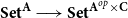so $ \Delta [P \otimes F]$ is the functor $ \textbf {Set}^{\textbf {A}} \longrightarrow \textbf {Set}^{\textbf {A}^{op} \times \textbf {C}}$ with values

\begin{equation*} \Delta [P \otimes F](\Phi ) (A, C) = \Delta _A [P \otimes F](\Phi ) (C) \rlap . \end{equation*}

On the other hand, $ P \otimes \Delta {[}F{]}$ is the composite

\begin{equation*} \textbf {Set}^{\textbf {A}} \xrightarrow{\Delta {[}F{]}} \textbf {Set}^{\textbf {A}^{op} \times \textbf {B}} \xrightarrow{P \otimes _{\textbf {B}} (\ \ )} \textbf {Set}^{\textbf {A}^{op} \times \textbf {C}} \end{equation*}

so has values

\begin{equation*} (P \otimes \Delta {[}F{]}) (\Phi ) (A, C) = (P \otimes _{\textbf {B}} (\Delta {[}F{]} (\Phi ))) (A, C) \rlap . \end{equation*}

By the definition of composition of profunctors, this is

\begin{equation*} \begin{array}{lll} & &\kern-2pc \int ^B P (B, C) \times \Delta {[}F{]} (\Phi ) (A, B)\\ & = & \int ^B P(B, C) \times \Delta _A [F] (\Phi ) (B)\\ & = & (P \otimes \Delta _A [F] (\Phi )) (C) \end{array} \end{equation*}

and by Proposition3.5 this is isomorphic to $ \Delta _A [P \otimes F] (\Phi ) (C)$ .

4.3 A natural reformulation

It will be conceptually clearer to reformulate the definition of $ \Delta$ in more categorical terms, that is, in terms of natural transformations, Yoneda style. This rids us of many of the element-based proofs, eliminating, as it does, membership and especially non-membership. The results are cleaner and clearer, especially in the next section where we see the chain rule reduced to composition. This is a vast improvement over the construction and proof of the one-variable chain rule given in Paré (2024) which is far from transparent.

So why not just start with this as a definition? The basic intuition of finite differences would be lost. It is hard to imagine why one would define a profunctor using (2) or (3) in the proposition below, or formulate the product and sum rules or the chain rule.

Proposition 4.6. Let $ F \colon \textbf {Set}^{\textbf {A}} \longrightarrow \textbf {Set}^{\textbf {B}}$ be a tense functor and $ \Phi$ an object of $ \textbf {Set}^{\textbf {A}}$ . Then there is a natural bijection between the following:

(1) Elements 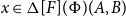$ x \in \Delta {[}F{]} (\Phi ) (A, B)$

(2) Natural transformations $ t \colon \textbf {B} (B, -) \longrightarrow F (\Phi + \textbf {A}(A, -))$ giving a pullback

(3) Natural transformations $ u \colon F(\Phi ) + \textbf {B}(B,-) \longrightarrow F (\Phi + \textbf {A} (A,-))$ giving a pullback

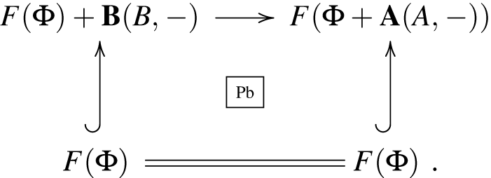
Proof. An element of $ \Delta {[}F{]} (\Phi ) (A, B)$ is an element of $ F (\Phi + \textbf {A} (A,-)) (B)$ , which is not in $ F (\Phi ) (B)$ . By Yoneda, this corresponds bijectively to a natural transformation

\begin{equation*} t \colon \textbf {B} (B, -) \longrightarrow F (\Phi + \textbf {A}(A,-)) \end{equation*}

for which $ t (B)(1_B) \notin F (\Phi )(B)$ . As is complemented by tenseness, that’s equivalent to none of the values of $ t$ being in $ F (\Phi )$ , which means that

is a pullback. And this, in turn, is equivalent to

being a pullback, where $ u$ is the inclusion on the first summand and $ t$ on the second.

As mentioned in Definition 1.1, it is useful to think of the elements of a profunctor as some sort of morphism but between objects of different categories (sometimes called heteromorphisms). Because of the representables appearing in the natural transformations above, it’s not unreasonable to think of them as morphisms from $ A$ to $ B$ , as a kind of Kleisli morphism although $ F$ is not a monad. If $ F$ were the identity for example, $ t$ is equivalent to a natural transformation $ \textbf {B}(B,-) \longrightarrow \textbf {A} (A,-)$ so to an actual morphism $ A \longrightarrow B$ . This is just another way of saying that $ \Delta [1_{\textbf {Set}^{\textbf {A}}}] (\Phi ) = {\textrm {Id}}_{\textbf {A}}$ , the identity profunctor on $ \textbf {A}$ , i.e., the hom functor.

More generally, if $ F$ preserves binary coproducts, a $ t$ as above corresponds to a natural transformation

\begin{equation*} \textbf {B}(B,-) \longrightarrow F(\textbf {A} (A,-))\rlap {\,,} \end{equation*}

another way of viewing the identity

\begin{equation*} \Delta {[}F{]} (\Phi ) = C\!or (F) \end{equation*}

of Proposition4.4.

With the natural transformation version of $ \Delta$ , it is easy to see how $ \Delta {[}F{]} (\Phi ) (A, B)$ is functorial in $ A$ and $ B$ . Given a $ t$ as in (2) and morphisms $ f \colon A' \longrightarrow A$ and $ g \colon B \longrightarrow B'$ , we get pullbacks

the third one because $ F$ is tense.

Similarly, functoriality in $ \Phi$ is clear. For $ \phi \colon \Phi \longrightarrow \Psi$ , we get pullbacks

again using tenseness of $ F$ .

The same goes for the functoriality in $ F$ . If $ \alpha \colon F \longrightarrow G$ is a tense transformation, we get pullbacks

Showing that $ \Delta {[}F{]} \colon \textbf {Set}^{\textbf {A}} \longrightarrow \textbf {Set}^{\textbf {A}^{op} \times \textbf {B}}$ is tense in this context is probably no easier than the element-wise proof given for Proposition4.2, but it may be more conceptual. It is a result we need if we want to iterate $ \Delta$ , as we do. So we reprove it.

The proof that $ \Delta {[}F{]}$ preserves the pullbacks of complemented subobjects is basically the same as in Proposition 4.2, but we reproduce it here without reference to particular differences or evaluation functors.

Let

be a pullback of complemented subobjects in $ \textbf {Set}^{\textbf {A}}$ and $ A$ an object of $ \textbf {A}$ . Consider the four squares in $ \textbf {Set}^{\textbf {B}}$

(1) and (4) are pullbacks by definition of $ \Delta$ and (2) because $ F$ is tense. As the pasted rectangle (1) + (2) is equal to (3) + (4), we get that (3) is also a pullback.

As $ \Delta {[}F{]}$ preserves pullbacks of complemented subobjects, it will take a complemented subobject to a mono, but we still have to prove that it’s complemented. We have to prove that for any $ f \colon A' \longrightarrow A$ and $ g \colon B \longrightarrow B'$ ,

is a pullback.

An element of $ \Delta [\Phi ] (A,B)$ is a natural transformation $ t \colon \textbf {B}(B,-) \longrightarrow F (\Phi + \textbf {A}(A,-))$ . To be in $ \Delta [\Phi _0] (A,B)$ means that it factors through . Referring to the following diagram

$ \Delta [\Phi ] (f,g) (t)$ is the composite of the left arrow with the two top arrows, and to say that it is in $ F(\Phi _0 + \textbf {A}(A',-))$ means that there is a $ u$ making the outside boundary commute. The square in a pullback because $ F$ is tense so there exists a unique $ u'$ as shown and as $ F (\Phi _0 + \textbf {A}(A,-))$ is complemented there exists a $ u''$ by Proposition2.2. So $ t$ factors through $ F(\Phi _0 + \textbf {A}(A,-))$ , which is what we wanted.

4.4 Lax chain rule

We saw in Paré (2024) that the chain rule for the single variable functorial difference was expressed as a laxity morphism rather than an isomorphism, and the same applies in the multivariable case. For tense functors $ F \colon \textbf {Set}^{\textbf {A}} \longrightarrow \textbf {Set}^{\textbf {B}}$ and $ G \colon \textbf {Set}^{\textbf {B}} \longrightarrow \textbf {Set}^{\textbf {C}}$ , we will construct a comparison transformation

\begin{equation*} \gamma (\Phi ) \colon \Delta [G] (F(\Phi )) \otimes _{\textbf {B}} \Delta {[}F{]} (\Phi ) \longrightarrow \Delta [GF](\Phi ) \end{equation*}

and establish associativity and unit laws for it. In fact, considering $ \Delta {[}F{]} (\Phi )$ as a profunctor may not mean much unless it composes like a profunctor. Otherwise, it is just an object of $ \textbf {Set}^{\textbf {A}^{op} \times \textbf {B}}$ .

The construction of $ \gamma$ in Paré (2024) is perhaps a bit opaque and the profunctor interpretation clarifies this. We’ll see that it is, in a sense, just composition as it should be.

In the previous section, we described the functoriality of $ \Delta$ in terms of the characterization (2) of Proposition4.6, but for the chain rule the characterization (3) is better, so we reformulate the functorialities in this context. As we will refer to it a lot, let us call a natural transformation $ t$ such that

is a pullback, a PPI transformation (for pullback preserves injections).

Functoriality of $ \Delta {[}F{]} (\Phi ) (A,B)$ , considered as a set of PPI transformations, is easy. It’s just composition with $ F (\Phi + \textbf {A} (f, -))$ and $ F (\Phi ) + \textbf {B}(g,-)$ respectively.

Functoriality in $ \Phi$ and $ F$ are a bit more complicated as the $ \Phi$ and $ F$ appear in both the domain and codomain of $ t$ . The following characterization will be useful, although it is nothing but a reformulation.

Proposition 4.7. Let $ t \colon F (\Phi ) + \textbf {B} (B,-) \longrightarrow F (\Phi + \textbf {A}(A,-))$ be a PPI transformation.

(1) If $ \phi \colon \Phi \longrightarrow \Psi$ is a natural transformation, then $ \Delta {[}F{]} (\phi ) (A,B) (t)$ is the unique PPI transformation $ t'$ such that

(2) If $ \alpha \colon F \longrightarrow G$ is a tense transformation, then $ \Delta [\alpha ] (\Phi ) (A,B) (t)$ is the unique PPI transformation $ t''$ such that

Theorem 4.2. For tense functors $ F \colon \textbf {Set}^{\textbf {A}} \longrightarrow \textbf {Set}^{\textbf {B}}$ and $ G \colon \textbf {Set}^{\textbf {B}} \longrightarrow \textbf {Set}^{\textbf {C}}$ , there is a natural transformation

\begin{equation*} \gamma \colon (\Delta [G] \circ F) \otimes \Delta {[}F{]} \longrightarrow \Delta [GF] \end{equation*}

which is

1. (1) natural in $ F$ and $ G$

2. (2) associative

3. (3) normal (invertible unitors)

Proof. $ \gamma$ is to be understood pointwise, i.e., as a profunctor morphism

\begin{equation*} \gamma (\Phi): \Delta[G](F(\Phi)) \otimes _{\textbf {B}} \Delta[F](\Phi)\longrightarrow \Delta[GF](\Phi)\end{equation*}

for each $ \Phi \in \textbf {Set}^{\textbf {A}}$ , and furthermore natural in that $ \Phi$ .

Let $ A \in \textbf {A}$ and $ C \in \textbf {C}$ . An element of

\begin{equation*} \big (\Delta [G] (F(\Phi )) \otimes _{\textbf {B}} \Delta {[}F{]} (\Phi )\big ) (A,C) \end{equation*}

is an equivalence class

where $ u$ and $ t$ are PPI transformations. Let $ \gamma (\Phi )(A,C) (u \otimes _B t) = G t \cdot u$ , which is indeed PPI:

We must show that $ \gamma (\Phi ) (A,C)$ is well defined. Suppose we have another pair of transformation related by a single morphism

This means that we have commutative squares

If we apply $ G$ to the second and paste it to the first, we get a commutative diagram which shows that $ G t \cdot u = G t' \cdot u'$ . It follows that $ \gamma (\Phi ) (A,C)$ is well defined.

Naturality in $ A$ and $ C$ is clear as it is just composition with $ F (\Phi + \textbf {A} (f, -))$ and $ F (\Phi ) + \textbf {C}(h,-)$ , respectively, and has nothing to do with the equivalence relation, which is localized at $ B$ . So, we get a profunctor morphism $ \gamma (\Phi )$ .

To show that $ \gamma$ is natural in $ \Phi$ , let $ \phi \colon \Phi \longrightarrow \Psi$ be a natural transformation and consider

where the vertical arrows are induced by $ \phi$ . If we chase an element $ u \otimes _B t$ in the domain, first around the left-bottom we get $ u' \otimes _B t'$ and then $ G t' \cdot u'$ where $ u'$ and $ t'$ are the unique PPI’s such that

On the other hand, going around the top-right we get $ G t \cdot u$ and then $ v'$ the unique PPI such that

If we apply $ G$ to the diagram for $ t'$ above and paste it to the one for $ u'$ , we see that $ G t' \cdot u'$ is such a $ v'$ , and so $ v' = G t' \cdot u'$ . This gives naturality in $ \Phi$ .

We can check naturality in $ F$ and $ G$ separately. First, let $ \alpha \colon F \longrightarrow F'$ be a tense natural transformation. We wish to show that

commutes. $ \alpha$ acting on an element $ u \otimes _B t$ of the domain gives $ u' \otimes _B t'$ which gets sent to $ G t' \cdot u'$ , where

On the other hand we first get $ G t \cdot u$ and then $ v'$ such that

Again, applying $ G$ to the square for $ t'$ and pasting to the one for $ u'$ , we see that $ v' = G u' \cdot t'$ , i.e., naturality in $ F$ .

For naturality in $ G$ , let $ \beta \colon G \longrightarrow G'$ be a tense natural transformation. We’ll show that

commutes. An element $ u \otimes t$ of the domain, goes down to $ u' \otimes t$ and then $ G' u' \cdot t$ for $ u'$ such that

$ u \otimes t$ goes across to $ G t \cdot u$ and then down to $ v'$ such that

If we paste the diagram for $ u'$ with the naturality square

and compare with the diagram for $ v'$ we see that $ v' = G' t \cdot u'$ , which gives naturality in $ G$ .

Let

\begin{equation*} \textbf {Set}^{\textbf {A}} {\xrightarrow{F\hspace{8pt}}} \textbf {Set}^{\textbf {B}} {\xrightarrow{\hspace{8pt}G\hspace{8pt}}} \textbf {Set}^{\textbf {C}} {\xrightarrow{\hspace{8pt}H\hspace{8pt}}} \textbf {Set}^{\textbf {D}} \end{equation*}

be tense functors. Associativity involves taking an element $ v \otimes u \otimes t$ of

\begin{equation*} \Delta [H] (GF(\Phi )) \otimes _{\textbf {B}} \Delta [G] (F\Phi ) \otimes _{\textbf {C}} \Delta {[}F{]} (\Phi ) \end{equation*}

at $ (A,D)$ and applying $ \gamma$ in two different ways to reduce it to elements of $ \Delta [HGF](\Phi )$ , and seeing that they are equal. This is for any PPI transformations

\begin{align*} t \colon F (\Phi ) + \textbf {B} (B,-) & \longrightarrow F (\Phi + \textbf {A} (A,-))\\[8pt] u \colon GF (\Phi ) + \textbf {C} (C,-) & \longrightarrow G(F(\Phi ) + \textbf {B} (B,-))\\[8pt] v \colon HGF (\Phi ) + \textbf {D} (D,-) &\longrightarrow H (GF(\Phi ) + \textbf {C} (C,-))\rlap. \end{align*}

And indeed, we get

For the unit laws, first assume that $ \textbf {B} = \textbf {A}$ and that $ F = {\textrm {id}}_{\textbf {Set}^{\textbf {A}}}$ . Then, $ \gamma (\Phi )$ takes the form

\begin{equation*} \gamma (\Phi ) \colon \Delta [G] \otimes _{\textbf {A}} \Delta [{\textrm {id}}_{\textbf {Set}^{\textbf {A}}}] (\Phi ) \longrightarrow \Delta [G] (\Phi ) \end{equation*}

and an element of the domain is an equivalence class $ u \otimes t$ for PPI’s

\begin{equation*} \Phi + \textbf {A} (A',-) \xrightarrow{\hspace{6pt}t\hspace{6pt}} \Phi + \textbf {A} (A,-) \quad G(\Phi ) + \textbf {C} (C,-) \xrightarrow{\hspace{6pt}u\hspace{6pt}} G(\Phi + \textbf {A}(A',-))\rlap . \end{equation*}

For $ t$ to be a PPI, it must be of the form

\begin{equation*} \Phi + \textbf {A}(A',-) \xrightarrow{\Phi + \textbf {A} (f,-)} \Phi + \textbf {A}(A,-) \end{equation*}

and every equivalence class has a unique representative where $ f$ is $ 1_A$ . Then, $ \gamma (\Phi )(u \otimes 1) = u$ gives our bijective right unitor.

For the left unitor, let $ \textbf {B} = \textbf {C}$ and $ G = {\textrm {id}}_{\textbf {Set}^{\textbf {C}}}$ . Then, $ \gamma$ takes the form

\begin{equation*} \gamma (\Phi ) \colon \Delta [{\textrm {id}}_{\textbf {Set}^{\textbf {C}}}] (F (\Phi ) \otimes \Delta {[}F{]} (\Phi )) \longrightarrow \Delta {[}F{]} (\Phi ) \end{equation*}

and an element of its domain is an equivalence class $ u \otimes t$ with PPI’s

\begin{equation*} F(\Phi ) + \textbf {C}(C',-) \xrightarrow{\hspace{5pt}t\hspace{5pt}} F(\Phi + \textbf {A} (A,-))\quad F(\Phi ) + \textbf {C} (C,-) \xrightarrow{\hspace{5pt}u\hspace{5pt}} F(\Phi ) + \textbf {C} (C',-) \end{equation*}

For $ u$ to be a PPI it must be of the form $ F(\Phi ) + \textbf {C}(g,-)$ . Again every equivalence class contains a unique representative with $ g = 1_C$ . Then,

\begin{equation*} \gamma (\Phi ) (1 \otimes t) = t \end{equation*}

gives the bijective unitor.

As stated, the lax chain rule is called lax just because what might have been hoped to be an isomorphism is merely a comparison morphism reducing a more complicated expression to a simpler one. But, if we reformulate it in terms of the tangent bundle of Section 4.1, we get an actual lax normal functor.

Recall that the tangent functor $ T [F]$

is given by

\begin{equation*} T [F] (\Phi , \Psi ) = (F(\Phi ), \Delta {[}F{]} (\Phi ) \otimes _{\textbf {A}} \Psi ) \rlap . \end{equation*}

If $ G \colon \textbf {Set}^{\textbf {B}} \longrightarrow \textbf {Set}^{\textbf {C}}$ is another tense functor, then the composite

\begin{equation*} T [G] \circ T[F] = (GF(\Phi ), \Delta [G] (F(\Phi )) \otimes _{\textbf {B}} \Delta {[}F{]} (\Phi ) \otimes _{\textbf {A}} \Phi ) \end{equation*}

and

\begin{equation*} (1_{GF(\Phi )}, \gamma (\Phi ) \otimes _{\textbf {A}} \Psi ) \colon T [G] \circ T[F] \longrightarrow T[GF] \end{equation*}

makes $ T \colon {\mathscr{T}}\ \textit {ense} \longrightarrow {\mathscr{T}}\ \textit {ense}$ into a lax normal functor. We omit the details that only involve the rearrangement of the facts proved in Theorem4.2.

5. Newton Series

5.1 Multivariable Newton series

The Newton series of a function of a real variable $ f \colon {\mathbb R} \longrightarrow {\mathbb R}$ is a discrete version of Taylor series. Its aim is to recover $ f$ from its iterated differences or to approximate $ f$ by polynomials. The formula is well known

\begin{align*} & \kern-2pc \sum _{n = 0}^\infty \frac {\Delta ^n {[}f{]} (0)}{n!} x^{\downarrow n}\\ =\ & \sum _{n = 0}^\infty \Delta ^n {[}f{]} (0) \binom {x}{n} \end{align*}

when $ x^{\downarrow n}$ is the falling power $ x (x - 1) \ldots (x - n + 1)$ and $ \binom {x}{n}$ is the “binomial coefficient” $ \frac {x (x - 1) \ldots (x - n + 1)}{n!}$ .

Although not so well known, a recursive argument produces a multivariable version: for $ f \colon {\mathbb R^n} \longrightarrow {\mathbb R}$ , we have

\begin{align*} &\kern-2pc \sum _{k_1, k_2, \ldots , k_n = 0}^\infty \frac {\Delta ^{k_1}_{x_1} \Delta ^{k_2}_{x_2} \cdots \Delta ^{k_n}_{x_n} {[}f{]} (0,\ldots , 0)}{k_1 ! k_2 ! \cdots k_n !} x_1^{\downarrow k_1} x_2^{\downarrow k_2} \cdots x_n^{\downarrow k_n}\\ = \ & \sum _{k_1, k_2, \ldots ,k_n = 0}^\infty \Delta ^{k_1}_{x_1} \Delta ^{k_2}_{x_2} \cdots \Delta ^{k_n}_{x_n} {[}f{]} (0,\ldots , 0) \binom {x_1}{k_1} \binom {x_2}{k_2} \cdots \binom {x_n}{k_n}\rlap {\ .} \end{align*}

In Paré (2024), we gave a categorified version for taut endofunctors of $ \textbf {Set}$ and showed that for analytic functors their Newton series converge to them. In fact this holds for a larger class of taut functors, which we call soft analytic. Not only that, the approximation alluded to above manifests itself as a categorical adjointness. In this section, we develop multivariable versions of these results.

5.2 Soft multivariable analytic functors

In order to categorify multivariable Newton series, we must modify the notion of $ \textbf {A}$ – $ \textbf {B}$ symmetric sequence to take into account the extra structure that the iterated differences have. We replace the category $ ! \textbf {A}$ of Fiore et al. (2008) by the larger category $ {\downarrow }\textbf {A}$ with the same objects, finite sequences $ \langle A_1, \ldots , A_n \rangle$ of objects of $ \textbf {A}$ , but where the morphisms

\begin{equation*} \langle A_1, \ldots , A_n \rangle \longrightarrow \langle C_1, \ldots C_m \rangle \end{equation*}

are pairs $ (\sigma , \langle\, f_j \rangle )$ such that $ \sigma \colon m \longrightarrow n$ is a surjection and $ \langle\, f_j \rangle$ is a family of morphisms indexed by $ m$

\begin{equation*} f_j \colon A_{\sigma j} \longrightarrow C_j \rlap {\ .} \end{equation*}

Composition is formally the same as for $ ! \textbf {A}$

\begin{equation*} (\tau , \langle g_k \rangle ) (\sigma , \langle\, f_j \rangle ) = (\sigma \tau , \langle g_k f_{\tau k} \rangle )\rlap {\ .} \end{equation*}

Whereas $ ! \textbf {A}$ is the free symmetric strict monoidal category generated by $ \textbf {A}$ , $ {\downarrow }\textbf {A}$ is the free symmetric monoidal category in which every object has a canonical cocommutative coassociative comultiplication.

Definition 5.1. A soft $ \textbf {A}$ – $ \textbf {B}$ -symmetric sequence is a profunctor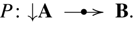

Given a soft $ \textbf {A}$ - $ \textbf {B}$ -symmetric sequence we define the functor $ \widetilde {P} \colon \textbf {Set}^{\textbf {A}} \longrightarrow \textbf {Set}^{\textbf {B}}$ by the formula

\begin{equation*} \widetilde {P} (\Phi )(B) = \int ^{\langle A_1 \ldots A_n\rangle \in {\downarrow }\textbf {A}} P(A_1, \ldots , A_n;\ B) \times \Phi A_1 \times {\ldots } \times \Phi A_n \rlap . \end{equation*}

Of course, for this to make sense $ \Phi A_1 \times {\ldots } \times \Phi A_n$ must come from a functor $ {\downarrow }\textbf {A} \longrightarrow \textbf {Set}$ , which is indeed the case. For a morphism,

\begin{equation*} (\sigma , \langle\, f_1 \ldots f_m\rangle ) \colon \langle A_1, \ldots , A_n \rangle \longrightarrow \langle C_1, \ldots , C_m \rangle \end{equation*}

we have a unique morphism making

commute for all $ j \in m$ .

A more conceptual description of $ \widetilde {P}$ is in terms of Kan extensions. Let $ Q \colon ({\downarrow }\textbf {A})^{op} \longrightarrow \textbf {Set}^{\textbf {A}}$ be the functor defined by

\begin{equation*} Q \langle A_1 {\ldots } A_n \rangle = \textbf {A} (A_1, -) + {\ldots } + \textbf {A} (A_n, -) \rlap {\ .} \end{equation*}

It is indeed a functor, its value on a morphism

\begin{equation*} (\sigma , \langle\, f_1, {\ldots } , f_m \rangle ) \colon \langle A_1, {\ldots } , A_n\rangle \longrightarrow \langle C_1, {\ldots } , C_m \rangle \end{equation*}

being the unique morphism making all the squares

commute. A profunctor is a functor $ P \colon ({\downarrow }\textbf {A})^{op} \times \textbf {B} \longrightarrow \textbf {Set}$ , which may be alternately described as a functor $ ({\downarrow }\textbf {A})^{op} \longrightarrow \textbf {Set}^{\textbf {B}}$ (which we denote by the same letter). Then, $ \widetilde {P}$ is the left Kan extension of $ P$ along $ Q$ :

Indeed,

\begin{equation*} \textrm {Lan}_Q P (\Phi ) = \int ^{A_1 {\ldots } A_n} P (A_1 {\ldots } A_n ; -) \times \textbf {Set}^{\textbf {A}} (Q \langle A_1, {\ldots } , A_n \rangle , \Phi ) \end{equation*}

(see Mac Lane (1971, p. 236)) and $ \textbf {Set}^{\textbf {A}} (Q \langle A_1 {\ldots } A_n \rangle , \Phi ) \cong \Phi A_1 \times {\ldots } \times \Phi A_n$ .

$ Q$ may be considered as a profunctor and we have the following “softening” of Proposition2.13.

Proposition 5.1.

1. 1. $ \widetilde {P}$ is the composite

   

2. 2. $ Q$ satisfies the condition of 2.4.1.

Proof. (1) Same as in Proposition 2.13.

(2) Again $ \pi _0 Q (A_1, {\ldots } , A_n ; -\!) = n$ for the same reason (sum of $ n$ representables), but now for a morphism $ (\sigma , \langle\, f_1 , {\ldots } , f_m \rangle ) \colon \langle A_1, {\ldots } , A_n \rangle \longrightarrow \langle C_1 , {\ldots } , C_m \rangle$ the morphism

\begin{equation*} \pi _0 Q (C_1, {\ldots } , C_m ; -) \longrightarrow \pi _0 Q (A_1 , {\ldots } , A_n ; -\!) \end{equation*}

is $ \sigma \colon m \longrightarrow n$ , which is onto.

Corollary 5.1. $ \widetilde {P}$ is tense.

A more elementary understanding of $ \widetilde {P}$ will be useful. From the coend formula for Kan extension, we see that an element of $ \widetilde {P} (\Phi ) (B)$ is an equivalence class of pairs $ (p, \phi )$

where $ p \in P (A_1, {\ldots } , A_n ;\, B)$ and $ \sum \textbf {A} (A_i, -)$ is short for $ \sum _{i = 1}^n \textbf {A} (A_i, -)$ . The equivalence relation is generated by identifying $ (p, \phi )$ and $ (q, \psi )$ when there is a morphism $ (\sigma , \langle\, f_j \rangle ) \colon \langle A_1 , {\ldots } , A_n \rangle \longrightarrow \langle C_1, {\ldots } , C_m \rangle$ in $ {\downarrow } \textbf {A}$ such that

where $ \sum _\sigma \textbf {A} (f_j, -)$ represents the natural transformation taking $ g \colon C_j {\xrightarrow{\hspace{8pt}A\hspace{8pt}}}$ to $ A_{\sigma (j)} {\xrightarrow{f_j}} C_j {\xrightarrow{\hspace{8pt}g\hspace{8pt}}} A$ .

Functoriality of $ \widetilde {P}$ in $ B$ and $ \Phi$ is by composition: for $ b \colon B \longrightarrow B'$

\begin{equation*} \widetilde {P} (\Phi ) (b) \colon (p, \phi ) \longmapsto (b p, \phi ) \end{equation*}

and for $ \theta \colon \Phi \longrightarrow \Psi$

\begin{equation*} \widetilde {P} (\theta )(B) \colon (p, \phi ) \longmapsto (p, \theta \phi ) \rlap {\ .} \end{equation*}

The universal property of Kan extensions says that for any functor $ F \colon \textbf {Set}^{\textbf {A}} \longrightarrow \textbf {Set}^{\textbf {B}}$ , we have a natural bijection

\begin{equation*} \widetilde {P} \xrightarrow{\hspace{5pt}t\hspace{5pt}} F \over P \xrightarrow{\hspace{5pt}u\hspace{5pt}} F Q \rlap {\ .} \end{equation*}

The correspondence between $ t$ and $ u$ is the following. $ t \colon \widetilde {P} \longrightarrow F$ is given by a family of natural transformations

\begin{equation*} \langle \widetilde {P} (\Phi ) \longrightarrow F (\Phi )\rangle _\Phi \end{equation*}

natural in $ \Phi \in \textbf {Set}^{\textbf {A}}$ , which further breaks down into a doubly indexed family of functions

\begin{equation*} \langle \widetilde {P} (\Phi ) (B) \longrightarrow F (\Phi ) (B) \rangle _{\Phi , B} \end{equation*}

natural in both $ \Phi$ and $ B$ . So for every equivalence class

we get an element $ t [p, \phi ] \in F (\Phi ) (B)$ .

On the other hand $ u \colon P \longrightarrow F Q$ is a doubly indexed family of functions

\begin{align*} \langle P(A_1, {\ldots }, A_n ;\, B) \longrightarrow F \Big(\sum \textbf {A} (A_i, -)\Big) (B) \rangle \end{align*}

natural in $ \langle A_1, {\ldots }, A_n\rangle \in \ {\downarrow }\textbf {A}$ and $ B$ in $ \textbf {B}$ .

Given $ t$ we get $ u$ by restricting to the case $ \Phi = \sum \textbf {A} (A_i, -)$ and $ \phi$ the identity

\begin{equation*} u (p) = t [p, {\textrm {id}}_{\sum \textbf {A} (A_i, -)}] \rlap {\ .} \end{equation*}

Given $ u$ we get $ t$ by

\begin{equation*} t [p, \phi ] = F (\phi ) (u (p)) \rlap {\ .} \end{equation*}

There is nothing to check, such as naturality or well-definedness, as it all follows by the general theory of Kan extensions. We will use these formulas in the proof of Theorem5.1.

Another result that will be useful is the following fact that, although trivial, is interesting in its own right and worth pointing out.

Lemma 5.1. For a pair , the Boolean image of $ \phi$

is an invariant of the equivalence class $ [p, \phi ]$ .

Proof. Suppose $ (p, \phi )$ and $ (q, \psi )$ are related by a single morphism $ (\sigma , \langle\, f_j\rangle )$ of $ {\downarrow }\textbf {A}$ , i.e.,

commute. Because $ (\sigma , \langle\, f_J\rangle )$ is in $ {\downarrow }\textbf {A}$ , $ \sum _\sigma \textbf {A} (f_j, -)$ is $ \pi _0$ -surjective, so $ \textrm {Bim} (\phi ) = \textrm {Bim} (\psi )$ .

Definition 5.2. A functor of the form $ \widetilde {P} \colon \textbf {Set}^{\textbf {A}} \longrightarrow \textbf {Set}^{\textbf {B}}$ for will be called soft analytic.

It will become clear below that $ P$ is uniquely determined by $ \widetilde {P}$ (see Theorem 5.2).

Proposition 5.2. Analytic functors are soft analytic.

Proof. The category $ ! \textbf {A}$ of Section 2.5 is a subcategory of $ {\downarrow }\textbf {A}$ , and the $ Q$ of Section 2.5, the restriction of the one just introduced. For an $ \textbf {A}$ - $ \textbf {B}$ symmetric sequence $ \widetilde {P}$ is the left Kan extension

which can be taken in stages giving, first a soft $ \textbf {A}$ - $ \textbf {B}$ symmetric sequence $ P'$ and then the analytic functor $ \widetilde {P}$ which is isomorphic to $ \widetilde {P}'$ .

We can describe $ P'$ explicitly. It’s the left Kan extension of $ P$ along the inclusion $ (!\textbf {A})^{op} \, \succ\!\xrightarrow{\hspace{.3cm}} \,({\downarrow }\textbf {A})^{op}$ so

\begin{equation*} P' (A_1 \ldots A_n;\ B) \cong \int ^{\langle C_1 \ldots C_m\rangle \in ! \textbf {A}} P (C_1 \ldots C_m ;\ B) \times {\downarrow }\textbf {A} (A_1 \ldots A_n;\ C_1 \ldots C_m) \rlap {\ .} \end{equation*}

An element of $ P' (A_1, \ldots , A_n ;\, B)$ is thus an equivalence class

where $ \sigma \colon m \twoheadrightarrow n$ is onto, $ f_j \colon A_{\sigma j} \longrightarrow C_j$ and $ p \in P (C_1 \ldots C_m ;\ B)$ . The equivalence relation is generated by identifying $ (\sigma , \langle\, f_j \rangle , p)$ with $ (\rho , \langle g_j \rangle , q)$ is there exists a morphism $ (\tau , \langle h_j \rangle )$ in $ !\textbf {A}$ such that

i.e.

In every equivalence class there are representatives of the form

and, after some calculation, we see that two such are equivalent if and only if there is a $ \tau \in S_m$ such that

We can further nail down the equivalence class by choosing canonical surjections $ m \twoheadrightarrow n$ , the order preserving ones, and these are determined by their fibres $ m_i$ which are positive integers. This gives a relatively simple description of $ P'$

\begin{equation*} P' (A_1, \ldots A_n ;\, B) \cong \sum _{m_1, \ldots m_n \gt 0} P (A_1^{\otimes m_1}, \ldots , A_n^{\otimes m_n} ;\ B) / S_{m_1} \times {\ldots } \times S_{m_n} \end{equation*}

where $ A_i^{\otimes m_i} = \langle A_i, A_i, \ldots , A_i \rangle \in \textbf {A}^{m_i}$ and the action is by permuting those entries.

5.3 The Newton series comonad

In this section, we show that taking iterated differences is right adjoint to summation of a multivariable symmetric series. We first combine all the iterated differences into one soft symmetric sequence.

Proposition 5.3. Let $ F \colon \textbf {Set}^{\textbf {A}} \longrightarrow \textbf {Set}^{\textbf {B}}$ be tense. Then taking the iterated symmetric differences of $ F$ evaluated at $ \Phi$ gives an $ \textbf {A}$ - $ \textbf {B}$ symmetric sequence

\begin{equation*} \Delta _* [F] (\Phi ) (A_1, \ldots , A_n ;\ B) = \Delta _{A_1} \ldots \Delta _{A_n} [F] (\Phi ) (B) \rlap {\ .} \end{equation*}

Proof. $ \Delta _{A_1} \ldots \Delta _{A_n} [F] (\Phi ) (B) = \Delta _{\langle A_i \rangle } [F] (\Phi )(B)$ consists of the new elements of

\begin{equation*} F(\Phi + \textbf {A} (A_1, -) + {\ldots } + \textbf {A} (A_n, -)) (B) \rlap {\ ,} \end{equation*}

i.e., those elements not in $ F( \Phi + \textbf {A} (A_{\alpha 1}, -) + {\ldots } + \textbf {A} (A_{\alpha k}, -))$ for any proper subsequence $ \langle A_{\alpha 1}, \ldots , A_{\alpha k} \rangle$ , a proper mono. We’ll show that $ \Delta _* [F]$ is a subfunctor of $ F(\Phi + Q)$ . Let $ (\sigma , \langle\, f_1, \ldots , f_m\rangle )) \colon \langle A_1, \ldots , A_n \rangle \longrightarrow \langle C_1, \ldots , C_m\rangle$ be a morphism in $ {\downarrow }\textbf {A}$ , and let $ x$ be an element of

\begin{equation*} \Delta _{C_1} \ldots \Delta _{C_m} [F] (\Phi ) (B) \subseteq F (\Phi + \textbf {A} (C_1, -) + {\ldots } + \textbf {A} (C_m, -)) (B)\rlap {\ .} \end{equation*}

Then, $ y = F (\sigma , \langle\, f_1, \ldots , f_m \rangle ) (B) (x)$ is an element of $ F (\Phi + \textbf {A} (A_1, -) + {\ldots } + \textbf {A} (A_n, -) (B)$ and suppose it’s not new. There is a proper monomorphism such that $ y \in F (\Phi _{\textbf {A}} (A_{\alpha 1}, -) + {\ldots } + \textbf {A} (A_{\alpha k}, -)) (B)$ .

The pullback of a proper mono along an epi is again proper so we get

which, in turn, gives a pullback of complemented subobjects in $ \textbf {Set}^{\textbf {A}}$

Adding $ \Phi$ produces another such pullback and $ F$ , being tense, will preserve it

Then, $ x$ in the upper right corner gets sent to $ y$ which is in the lower left corner, so $ x$ itself is in the upper left corner, i.e., $ x$ wasn’t new after all. Thus, $ \Delta _* [F] (\Phi )$ is a subfunctor of $ F (\Phi + Q)$ .

$ \Delta _* [F] (\Phi )$ is functorial in $ F$ . Indeed, applying Proposition3.1 recursively, we see that any tense transformation $ t \colon F \longrightarrow G$ restricts to

which will be natural and functorial automatically. Thus, for each $ \Phi$ in $ \textbf {Set}^{\textbf {A}}$ , we get a functor

\begin{equation*} \Delta [\ \ ] (\Phi ) \colon {\mathscr{T}}\ \textit {ense} (\textbf {Set}^{\textbf {A}}, \textbf {Set}^{\textbf {B}}) \longrightarrow {\mathscr{P}}{\kern.5pt}\textit {rof} ({\downarrow } \textbf {A}, \textbf {B}) \rlap {\ ,} \end{equation*}

i.e., $ \Delta _* [F] (\Phi )$ is an $ \textbf {A}$ - $ \textbf {B}$ soft symmetric sequence.

The main result of this section is the following:

Theorem 5.1.

\begin{align*} \Delta _* [\ \ ] (0) \ is\ right\ adjoint\ to\ \tilde {(\ )} \rlap {\ .} \end{align*}

Proof. $ \widetilde {P}$ is the left Kan extension of $ P$ along $ Q$

so for any functor $ F \colon \textbf {Set}^{\textbf {A}} \longrightarrow \textbf {Set}^{\textbf {B}}$ , we have a bijection

\begin{equation*} \widetilde {P} \xrightarrow{t} F \over P \xrightarrow{u} FQ \end{equation*}

as discussed above. Now $ \Delta _* [F] (0)$ is a subfunctor of $ F Q$ . Indeed

\begin{equation*} \Delta _* [F] (0) \langle A_1, \ldots , A_n \rangle (B) = \Delta _{A_1} \ldots \Delta _{A_n} [F] (0) (B) \end{equation*}

consists of the new elements of

\begin{equation*} F(Q \langle A_1, \ldots , A_n \rangle ) (B) = F (\textbf {A} (A_1, -) + {\ldots } + \textbf {A}(A_n, -))(B) \rlap {\ .} \end{equation*}

We’ll show that $ t \colon \widetilde {P} \longrightarrow F$ is tense if and only if $ u$ factors through , which will establish the theorem.

First assume $ t$ is tense. Let $ p$ be in $ P (A_1, \ldots , A_n ;\, B)$ so $ u (p)$ is in $ F (\textbf {A} (A_1, -) + {\ldots } + \textbf {A} (A_n, -)) (B)$ and assume $ u (p)$ is in $ F$ of some subsum $ F (\textbf {A} (A_{\alpha 1}, -) + {\ldots } + \textbf {A} (A_{\alpha k} , -)) (B)$ for a subset $ \alpha \colon k \, \succ\!\xrightarrow{\hspace{.3cm}} \, n$ of the indices. Tenseness of $ t$ applied to the complemented subsum gives a pullback

Then, $ u (p) = T [p, {\textrm {id}}_{\sum \textbf {A}(A_i, -)}]$ is in $ F(\sum \textbf {A} (A_{\alpha i}, -)) (B)$ so $ [p, {\textrm {id}}]$ is in the lower left corner, which means there are and $ \psi \colon \sum \textbf {A} (C_i, -) \longrightarrow \sum \textbf {A} (A_{\alpha i}, -)$ such that $ [q, \mu \psi ] = [p, {\textrm {id}}]$ . Thus, by Lemma5.1, we see that $ \textrm {Bim} (\mu \psi ) = \textrm {Bim} ({\textrm {id}}) = \sum \textbf {A}(A_i, -)$ . It follows that $ \mu$ is the identity, so $ u (p)$ is not contained in $ F$ of any proper subsum, i.e., is new. This gives our factorization of $ u$ through $ \Delta _* [F] (0)$ .

Conversely, assume that $ u$ factors through $ \Delta _* [F] (0)$ . We’ll show that $ t$ is tense. Let be a complemented subobject. We must show that

(*)

is a pullback. Take an element of $ \widetilde {P} (\Phi ) (B)$ and assume $ t (\Phi ) [p, \phi ] = F (\phi ) (p)$ is in $ F (\Psi )$ . Form the pullback

It is induced by a monomorphism $ \alpha \colon m \, \succ\!\xrightarrow{\hspace{.3cm}} \, n$ because a complemented subobject of a sum of representables is a subsum. We get a new pullback now by tenseness of $ F$

$ F (\phi )$ takes $ u (p)$ to an element of $ F(\Psi )$ so $ u (p) \in F (\sum \textbf {A}(A_{\alpha j}, -))$ . But $ u (p)$ was supposed to be a new element of $ F(\sum \textbf {A} (A_i, -))$ so $ \alpha$ is not a proper subsum which means that

Thus $ [p, \phi ]$ is in $ \widetilde {P} (\Psi )$ . This shows that our square $ (*)$ is indeed a pullback.

The adjoint pair $ \tilde {(\ )} \dashv \Delta _* [\ \ ] (0)$ induces a comonad on $ {\mathscr{T}}\textit{ense} (\textbf {Set}^{\textbf {A}}, \textbf {Set}^{\textbf {B}})$ , which we call the Newton series comonad.

5.4 Convergence

In this section, we show that the Newton series for a soft analytic functor “converges to it”.

Theorem 5.2. For every $ \textbf {A}$ - $ \textbf {B}$ soft symmetric sequence , the unit for the adjunction of Theorem 5.1

\begin{equation*} P \longrightarrow \Delta _* [\widetilde {P}] (0) \end{equation*}

is an isomorphism.

Proof. An element of $ \Delta _* [\widetilde {P}] (0)$ at $ \langle A_1, \ldots , A_n \rangle , B$ is a new element of $ \ \widetilde {P} (\sum \textbf {A}(A_i, -)) (B)$ , i.e., of

\begin{align*} \int ^{C_1, \ldots , C_m \in {\downarrow } \textbf {A}} P (C_1, \ldots , C_m;\ B) \times \textbf {Set}^{\textbf {A}} \Big(\sum \textbf {A}(C_j, -), \sum \textbf {A} (A_i, -)\Big) \end{align*}

which is an equivalence class

(satisfying the newness condition, of course).

The unit $ P \longrightarrow \Delta _* [\widetilde {P}] (0)$ takes to the equivalence class

A $ \phi$ as above is, as explained in the discussion around Proposition2.4, of the form $ \sum _\alpha \textbf {A} (f_j, -)$ for $ \alpha \colon m \longrightarrow n$ and $ f_j \colon A_{\alpha j} \longrightarrow C_j$ , and we can take its Boolean factorization by factoring $ \alpha$ (in $ \textbf {Set}$ )

and taking

If $ \mu$ were a proper mono, $ [p, \phi ]$ wouldn’t be new as it would be in $ \widetilde {P} (\sum _{i \in k} \textbf {A} (A_{\mu i}, -))$ , so $ \mu = {\textrm {id}}_n$ and $ \alpha = \sigma$ , a surjection. Thus, $ (\sigma , \langle\, f_1\rangle )$ is a morphism of $ {\downarrow } \textbf {A}$ , and we have

so $ [p, \phi ] = [p', {\textrm {id}}]$ , which shows that the unit

\begin{equation*} P \longrightarrow \Delta _* [\widetilde {P}] (0) \end{equation*}

\begin{equation*} p \longmapsto [p, {\textrm {id}}] \end{equation*}

is onto.

To show that the unit is one-one, we must show that if $ [p, {\textrm {id}}] = [q, {\textrm {id}}]$ then $ p = q$ . $ [p, {\textrm {id}}] = [q, {\textrm {id}}]$ means there’s a zigzag path of

with $ (\rho , \langle h_j\rangle )$ in $ {\downarrow }\textbf {A}$ joining $ [p, {\textrm {id}}]$ to $ [q, {\textrm {id}}]$ . The Boolean image of $ \phi _i$ (and $ \psi _i$ ) is an invariant of the equivalence class (Lemma 5.1) and as $ \textrm {Bim} ({\textrm {id}}) = \sum \textbf {A} (A_i, -)$ , all the $ \phi$ and $ \psi$ also have $ \sum \textbf {A} (A_i, -)$ as their images. That means that the morphisms $ (\sigma , \langle\, f_j \rangle )$ and $ (\tau , \langle g_s \rangle )$ corresponding to $ \phi$ and $ \psi$ are actually morphisms in $ {\downarrow } \textbf {A}$ , i.e., $ \sigma \colon m \longrightarrow n$ and $ \tau \colon r \longrightarrow n$ are surjections. Now we have

commuting $ {\bar {p}} (\sigma , \langle\, f_j\rangle ) = {\bar {q}} ( \tau , \langle g_s\rangle )$ at every stage of the path joining $ (p, {\textrm {id}})$ to $ (q, {\textrm {id}})$ , and for these endpoints we get $ p$ and $ q$ respectively, i.e., $ p = q$ .

This shows that the Newton series comonad is idempotent.

Corollary 5.2. If $ F \colon \textbf {Set}^{\textbf {A}} \longrightarrow \textbf {Set}^{\textbf {B}}$ is soft analytic (in particular analytic) then its Newton series converges to it, i.e., the counit

\begin{equation*} \widetilde {\Delta _*[F](0)} \longrightarrow F \end{equation*}

is an isomorphism.

5.5 Concluding remark

In the previous sections, we touted the functor taking $ F$ to $ {\bar {F}} = \widetilde {\Delta _* [F] (0)}$ as a categorical version of the Newton summation formulas at the beginning of Section 5.1, but in fact, it looks nothing like them.

Let’s consider the first one

\begin{equation*} {\bar {f}} (x_1, \ldots , x_n) = \sum _{k_1, \ldots , k_n} \frac {\Delta ^{k_1}_{x_1} {\ldots } \Delta ^{k_n}_{x_n} [f] (0, \ldots , 0)} {k_{1!} \ldots k_{n!}} \ x^{\downarrow k_1}_1 \ldots x^{\downarrow k_n}_n \end{equation*}

where $ f$ is a function $ {\mathbb R}^n \longrightarrow {\mathbb R}$ and the sum is taken over all $ n$ -tuples of natural numbers. We’ve replaced $ f$ by a (tense) functor $ \textbf {Set}^{\textbf {A}} \longrightarrow \textbf {Set}^{\textbf {B}}$ and the difference operators by our functorial ones, but it’s not clear how to interpret the rest of the formula. Let’s look at it more carefully.

The first thing to note is that, while the $ x_i$ in $ \Delta _{x_i}$ and in $ x_i^{\downarrow k_i}$ refer to the same thing, they play different roles. The $ x_i$ in $ \Delta _{x_i}$ is merely a subscript indicating which difference operator is used, and we could well have written $ \Delta _i$ instead, although $ \Delta _{x_i}$ is more descriptive. The $ x_i$ in $ x_i^{\downarrow k_i}$ , on the other hand, represents a variable which can take values, $ c_i$ . So we have

\begin{equation*} {\bar {f}} (c_1, \ldots , c_n) = \sum _{k_1, \ldots , k_n} \frac {\Delta ^{k_1}_{x_1} {\ldots } \Delta ^{k_n}_{x_n} [f] (0, \ldots , 0)} {k_{1!} \ldots k_{n!}} \ c^{\downarrow k_1}_1 \ldots c^{\downarrow k_n}_n \rlap {\ .} \end{equation*}

Here, all the like $ \Delta$ ’s have been grouped together that is fine as we have finitely many variables, and they’re totally ordered. It would be more natural to sum over all finite sequences of variables $ \langle x_{\alpha (1)} \ldots x_{\alpha (m)} \rangle$ and group the terms together by the length $ m$ . Of course, we get more terms: $ \Delta ^{k_1}_{x_1} \ldots \Delta ^{k_n}_{x_n}$ gets counted

\begin{equation*} \binom {k_1 + {\ldots } + k_n}{k_1, \ldots , k_n} \ =\ \frac {(k_1 + {\ldots } + k_n)!}{k_1 ! \ldots k_n !} \ =\ \frac {m !}{k_1 ! \ldots k_n !} \end{equation*}

times, so now we have

\begin{equation*} {\bar {f}} (c_1, \ldots , c_n) = \sum _{\alpha \colon m \longrightarrow n} \frac {\Delta _{\alpha (1)} \ldots \Delta _{\alpha (m)} [f] (0, 0)} {m !} \ c^{\downarrow k_1}_1 \ldots c^{\downarrow k_n}_n \rlap {\ .} \end{equation*}

In fact this takes care of the finiteness and total ordering of the variables, as far as the $ \Delta$ part of the formula is concerned. We take a set of variables $ \textrm {Var}$ and consider the free monoid on it $ \textrm {Var}^*$ , over which the sum is to be taken. The $ c_i$ are a choice of value for each variable $ \phi \colon \textrm {Var} \longrightarrow {\mathbb R}$ , but we still have to deal with the $ k_i$ in this setup.

The $ k$ ’s count the number of occurrences of a given variable $ y$ in a sequence $ \langle x_1, \ldots , x_n\rangle$ . Let

\begin{equation*} \delta \colon \textrm {Var} \times \textrm {Var} \longrightarrow {\mathbb N} \end{equation*}

be the Kronecker delta, i.e., $ \delta (x, y) = 1$ if $ x = y$ and $ 0$ otherwise. For each $ y$ , extend $ \delta (-, y)$ to a function $ \delta (-, y) \colon \textrm {Var}^* \longrightarrow {\mathbb N}$ using the additive structure of $ {\mathbb N}$ , so

\begin{equation*} \delta (x_1, \ldots , x_n;\ y) = \sum ^m_{i = 1} \delta (x_i, y) \end{equation*}

is exactly the number of $ y$ ’s in $ \langle x_1, \ldots , x_n\rangle$ . Thus, we end up with the Newton series in the form we want

\begin{equation*} {\bar {f}} (\phi ) = \sum _{\langle x_1, \ldots , x_n\rangle \in \textrm {Var}^*} \frac {\Delta _{x_1} \ldots \Delta _{x_m} [f](0)}{m !} \prod _{y \in \textrm {Var}} \phi (y)^{\downarrow \delta (x_1, \ldots x_n ;y)} \end{equation*}

which, admittedly, looks more complicated than the original, but it’s the closest we can get to the categorical version.

Now the Newton series comonad of Section 5.3

\begin{equation*} \widetilde {\Delta _*[F] (0)} = \int ^{\langle A_1, \ldots , A_m\rangle \in \downarrow \textbf {A}} \Delta _{A_1} \ldots \Delta _{A_m} [F] (0) \times \textbf {Set}^{\textbf {A}} (\textbf {A} (A_1, -) + {\ldots } + \textbf {A} (A_m, -), \Phi ) \end{equation*}

looks similar to the above, with the following correspondences:

\begin{equation*} \begin{array}{rcl} f \colon {\mathbb R}^n \longrightarrow {\mathbb R} & \leftrightarrow & F \colon \textbf {Set}^{\textbf {A}} \longrightarrow \textbf { Set}^{\textbf {B}}\\ \mbox{variables } x & \leftrightarrow & \mbox{objects } A \mbox{ of } \textbf { A}\\ \textrm {Var} & \leftrightarrow & \textbf {A}\\ \textrm {Var}^* & \leftrightarrow & {\downarrow }\textbf {A}\\ \phi \colon \textrm {Var} \longrightarrow {\mathbb R} & \leftrightarrow & \Phi \colon \textbf {A} \longrightarrow \textbf {Set}\\ \delta (x, y) & \leftrightarrow & \textbf {A} (A', A)\\ \delta (x_1, \ldots , x_n, y) & \leftrightarrow & \textbf {A} (A_1, A) + {\ldots } + \textbf { A} (A_m, A)\\ \prod {\phi (y)}^{\downarrow \delta (x_1 \ldots x_n;y)} & \leftrightarrow & \textbf {Set}^{\textbf {A}} (\textbf {A} (A_1, -)+ {\ldots } + \textbf {A} (A_m, -), \Phi ) \end{array} \end{equation*}

The correspondence is not perfect, of course. $ \textrm {Var}^*$ might rightly be said to correspond to $ ! \textbf {A}$ rather than $ {\downarrow } \textbf {A}$ . Then, the $ m !$ in the sum is incroporated in the coend via the symmetric groups.

Also $ \prod \phi (y)^{\downarrow \delta (x_1, \ldots , x_m, y)}$ should correspond to monomorphisms

\begin{equation*} \textbf {A} (A_1, -) + {\ldots } + \textbf {A} (A_m, -) \longrightarrow \Phi \end{equation*}

rather than arbitrary natural transformations. That’s what the extra morphisms in $ {\downarrow }\textbf {A}$ (involving surjections $ \sigma$ ) take care of. We need a bit more theory to explain this.

Definition 5.3. Let $ \Phi \colon \textbf {A} \longrightarrow \textbf {Set}$ and $ x \in \Phi A$ . An ancestor of $ x$ is a $ y \in \Phi A'$ for which there is a morphism $ f \colon A' \longrightarrow A$ such that $ \Phi (f)(y) = x$ . Two elements $ x_1 \in \Phi A_1$ and $ x_2 \in \Phi A_2$ are relatives if they have a common ancestor. A sequence $ \langle x_1 \in \Phi A_1, \ldots , x_n \in \Phi A_n \rangle$ is called diverse if no two elements are relatives. A natural transformation $ \phi \colon \sum \textbf {A} (A_i, -) \longrightarrow \Phi$ is diverse if the corresponding sequence of elements $ \langle \phi (A_i) (1_{A_i}) \rangle$ is.

All the elements of a diverse sequence are different and more, but not enough more to make the corresponding transformation monic. One could have $ i \neq j$ and $ f \colon A_i \ \longrightarrow A, g \colon A_j \longrightarrow A$ with $ \Phi (f) (x_i) = \Phi (g) (x_j)$ . But if $ \textbf {A}$ is a groupoid, then $ \phi$ is monic if and only if it is diverse. The variables $ x_1, \ldots , x_n$ in the formula we’re abstracting from form a finite discrete set so diverse restricts to one-one in that case.

Proposition 5.4.

1. (1) $ \phi$ as below is diverse if and only if for every factorization of $ \Phi$

   

   with $ (\sigma , \langle\, f_i\rangle ) \colon \langle C_1, \ldots , C_m \rangle \longrightarrow \langle A_1, \ldots , A_n \rangle$ in $ {\downarrow } \textbf {A}$ , we have that $ \sigma$ is a bijection, i.e., $ (\sigma , \langle\, f_i\rangle ) \in ! \textbf {A}$ .

2. (2) Every $ \phi$ factors as $ \psi \sum _\sigma \textbf {A} (f_i, -)$ with $ (\sigma , \langle\, f_i\rangle ) \in {\downarrow }\textbf {A}$ and $ \psi$ diverse.

Proof. (1) $ \phi$ and $ \psi$ as in the statement correspond to an $ n$ -tuple $ x_1 \in A_1, \ldots , x_n \in \Phi A_n$ and an $ m$ -tuple $ y_1 \in \Phi C_1, \ldots , y_m \in \Phi C_m$ , respectively. The $ x$ ’s and $ y$ ’s are related by

\begin{equation*} x_i = \Phi (f_i) (y_{\sigma i}) \rlap {\ .} \end{equation*}

If $ \sigma$ is not one-to-one, say $ \sigma (i_1) = \sigma (i_2)$ , then $ x_{i_1}$ and $ x_{i_2}$ are relatives as they have the common ancestor $ y_{\sigma (i_1)} = y_{\sigma (i_2)}$ . So, the $ x_i$ are not diverse nor is $ \phi$ .

Conversely, if the $ x_i$ are not diverse, then there are two $ x$ ’s that are relatives. Assume, for simplicity of notation, that they are $ x_{n - 1}$ and $ x_n$ . So, we have $ f \colon C \longrightarrow A_{n - 1}, g \colon C \longrightarrow A_n$ and $ y \in \Phi C$ such that $ \Phi (f) (y) = x_{n - 1}$ and $ \Phi (g) (y) = x_n$ . Then, we get a morphism

\begin{equation*} (\sigma , \langle\, f_i\rangle ) \colon \langle A_1, \ldots , A_{n - 2}, C \rangle \longrightarrow \langle A_1, \ldots , A_n \rangle \end{equation*}

\begin{equation*} \sigma (i) = \left \{ \begin{array}{lcl} i & \mbox{if} & i \lt n\\ n -1 & \mbox{if} & i = n \rlap {\ ,} \end{array} \right . \end{equation*}

\begin{equation*} \langle\, f_i \rangle = \langle 1_{A_1}, \ldots , 1_{A_{n - 2}}, f, g\rangle \rlap {\ .} \end{equation*}

Let $ \langle y_1, \ldots , y_{n - 1} \rangle = \langle x_1, \ldots , x_{n - 2}, y \rangle$ . Then,

\begin{equation*} x_i = \Phi (f_i) (y_{\sigma i}) \end{equation*}

so the $ y$ determine a $ \psi$ giving a factorization as above, and $ \sigma$ is not a bijection.

This proves (1).

(2) If $ \phi$ is not diverse, there exists a factorization as in (1) with $ \sigma$ onto but not one-to-one, so $ \sum \textbf {A} (C_j, -)$ has fewer terms than $ \sum \textbf {A} (A_i, -)$ . If we take, among all factorizations, one with the minimal number of terms, the $ \psi$ must be diverse, otherwise we could factor it again and get a smaller one.

Corollary 5.3. Every equivalence class

\begin{align*} \Big[ x \in F \Big(\sum \textbf {A} (A_i, -)\Big) (B), \phi \colon \sum \textbf {A} (A_i, -) \longrightarrow \Phi \Big] \end{align*}

in

\begin{equation*} \int ^{\langle A_1, \ldots , A\rangle \in {\downarrow }\textbf {A}} \Delta _{A_1} \ldots \Delta _A [F] (0) (B) \times \textbf {Set}^{\textbf {A}} \Big(\sum \textbf {A} (A_i, -), \Phi \Big) \end{equation*}

has a representative in which $ \phi$ is diverse.

Proof. Factor $ \phi$ as in Proposition 5.4 (2) above. Then

so $ [x, \phi ] = [y, \psi ]$ and $ \psi$ is diverse.

The diverse transformations are our categorified set injections so

\begin{align*} \mbox{Diverse}\ \bigg(\sum \textbf {A} (A_i, -), \Phi \bigg) \end{align*}

is our version of falling power. Note, however, that it is not functorial, and we need all transformations to make it so.