


1. Introduction
In the analysis of large-scale wireless network performance, a critical metric, known as the meta distribution (MD), has emerged as a cornerstone in revealing the performance of individual links [Reference Haenggi5, Reference Haenggi7, Reference Haenggi8]. MDs play a key role in dissecting the impact of different sources of randomness on network performance. Quantities that affect the quality of the service of the users, such as signal power, signal-to-interference ratio (SIR), instantaneous rate, or energy, are inherently random, and we call them performance random variables (PRVs) [Reference Wang and Haenggi27]. Because of the nature of wireless networks, the PRVs strongly depend on user locations and are also time-varying, in other words, different sources of randomness. In this context, the MD emerges as a powerful tool to disentangle the different sources of randomness by analyzing the distribution of conditional probabilities.
However, calculating MDs is far from trivial. In some simplified network models, closed-form expressions can be obtained [Reference Haenggi7], but in more complete models, directly deriving analytic expressions is most likely impossible [Reference Haenggi5, Reference Tang, Xu and Haenggi26, Reference Wang, Cui, Haenggi and Tan29]. Thankfully, with the tool of stochastic geometry, the moments of the underlying conditional probabilities can be calculated [Reference Haenggi5, Reference Tang, Xu and Haenggi26, Reference Wang, Cui, Haenggi and Tan29]. Thus, we take a detour to calculate the distribution from its integer moments, which is a classical moment problem, called the Hausdorff moment problem (HMP) [Reference Hausdorff9, Reference Markov14, Reference Schmüdgen21, Reference Shohat and Tamarkin23]. The HMP seeks to ascertain whether a particular sequence corresponds to the integer moments of a valid random variable [Reference Hausdorff9, Reference Schmüdgen21, Reference Shohat and Tamarkin23], in other words, the existence of a solution (as a random variable) whose integer moments match a given sequence. The existence condition is that the given sequence is completely monotonic (c.m.) [Reference Hausdorff9, Reference Schmüdgen21, Reference Shohat and Tamarkin23]. When this criterion is met, a solution exists, and it is unique [Reference Hausdorff9, Reference Schmüdgen21, Reference Shohat and Tamarkin23]. The HMP is also relevant in many fields other than the MDs in wireless networks, such as the density of states in a harmonic solid (see, e.g., [Reference Mead and Papanicolaou16]), and particle size distributions (see, e.g., [Reference John, Angelov, Öncül and Thévenin11]). From a probability theory perspective, the existence of a solution is the primary concern, however, in practical applications, we know a priori that solutions exist, since the sequences are derived from random variables. Therefore, the target is to find the solution—in other words, to invert the mapping from a probability distribution to its moments. Given any tolerance greater than 0, we can approximate the solution within this tolerance (as measured by a suitable distance metric) using finitely many integer moments. Related, in practical scenarios, it is possible that only a finite number of integer moments can be calculated. Both aspects lead us to consider the truncated HMP (THMP).
The THMP diverges from the HMP in its objective. The former seeks solutions or approximations when the given finite-length sequence is from a valid moment sequence [Reference Schmüdgen21, Reference Shohat and Tamarkin23], while the latter focuses on the existence and uniqueness of the solution for a given infinite-length sequence [Reference Shohat and Tamarkin23]. Further complicating matters, the THMP usually yields infinitely many solutions when the given sequence is valid [Reference Schmüdgen21, Reference Shohat and Tamarkin23]. More importantly, solutions or approximations to the THMP are approximations to the HMP. We call a method that finds a solution or approximates a solution to the THMP a Hausdorff moment transform (HMT).
In the context of practical applications, such as MDs, the density of states in a harmonic solid, and particle size distributions, the sequences applied to the THMP can theoretically be extended to any length; therefore, our primary focus centers on the ultimate behavior of the HMTs as the lengths of the sequences increase. Various HMTs to the THMP have been proposed in the literature [Reference Guruacharya and Hossain4, Reference Markov14, Reference Mead and Papanicolaou16, Reference Mnatsakanov and Ruymgaart18, Reference Schoenberg22–Reference Szegö24], but there is a gap between developing the HMTs and applying them to solve practical problems. More specifically, the choice of the appropriate HMT is not clear. Different HMTs may exhibit varying effectiveness in different scenarios, giving rise to the need for a method of comparison that allows fair evaluationFootnote 1 and informed decision-making.
In this study, we bridge this gap by introducing a systematic and comprehensive method of comparison for HMTs, based on their accuracy, computational complexity, and precision requirements. This way, the most suitable HMT for given objectives can be chosen. The key point to make fair comparisons is to generate representative moment sequences. Generating random moment sequences is non-trivial since the probability that an unsorted sequence of length n with each element independent and identically distributed (i.i.d.) uniformly on  $[0,1]$ is a moment sequence is approximately $2^{-n^2}$ [Reference Chang, Kemperman and Studden1, Eq. 1.2] and the probability that a sorted sequence of length n with each element i.i.d. uniformly on $[0,1]$ is a moment sequence is approximately $n!2^{-n^2}$. We provide three different ways to solve it: One is to generate random integer moment sequences that are uniformly distributed in the moment space; the other two are based on analytic expressions, either of moments or of the cumulative distribution functions (cdfs). Moreover, our contributions extend to the enhancement of existing HMTs on the implementation front, improving them with heightened efficiency and practical applicability. In particular, we write some of the HMTs as linear transforms, which significantly lower their computational complexity and enable carrying out the most computationally intensive tasks offline.
2. Preliminaries
2.1. The Hausdorff moment problem
Without loss of generality, we assume the support of the distributions is  $[0,1]$. The THMP can be formulated as follows. Let $[n] \triangleq \{1,2,...,n\}$ and $[n]_0 \triangleq \{0\} \cup [n]$. Given a sequence
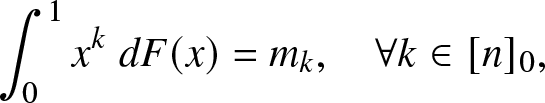
  $\mathbf{m} \triangleq (m_k)_{k=0}^{n}, \, n \in \mathbb{N}$, find or approximate an F such that
 \begin{align}
\int_{0}^{1} x^k \;dF(x) = m_k, \quad \forall k \in [n]_0,
\end{align}
\begin{align}
\int_{0}^{1} x^k \;dF(x) = m_k, \quad \forall k \in [n]_0,
\end{align} where F is right-continuous and increasing with  $F(0^-) = 0$ and $F(1) = 1$, that is, F is a cdf.
Although in practical applications, we are not concerned with the existence and uniqueness of the solutions to the THMP, we still find it valuable to examine these conditions to account for scenarios where the moments may not be exact.
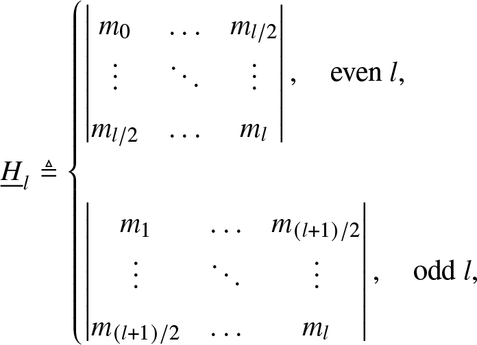
Let  $\mathcal{F}_n$ be the family of F that solves (2.1). The existence and uniqueness of solutions can be verified by the Hankel determinants, defined by
 \begin{align}
\underline{H}_{l} & \triangleq
\begin{cases}
\begin{vmatrix}
m_0 & \dots & m_{l/2} \\
\vdots & \ddots & \vdots \\
m_{l/2} & \dots & m_{l}
\end{vmatrix}, \quad\text{even } l,\\
\\
\begin{vmatrix}
m_1 & \dots & m_{(l+1)/2} \\
\vdots & \ddots & \vdots \\
m_{(l+1)/2} & \dots & m_{l}
\end{vmatrix}, \quad\text{odd }l,
\end{cases}
\end{align}
\begin{align}
\underline{H}_{l} & \triangleq
\begin{cases}
\begin{vmatrix}
m_0 & \dots & m_{l/2} \\
\vdots & \ddots & \vdots \\
m_{l/2} & \dots & m_{l}
\end{vmatrix}, \quad\text{even } l,\\
\\
\begin{vmatrix}
m_1 & \dots & m_{(l+1)/2} \\
\vdots & \ddots & \vdots \\
m_{(l+1)/2} & \dots & m_{l}
\end{vmatrix}, \quad\text{odd }l,
\end{cases}
\end{align}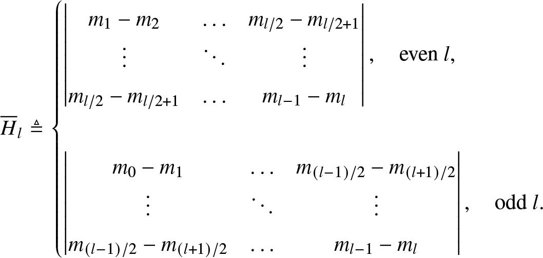 \begin{align}
\overline{H}_l & \triangleq
\begin{cases}
\begin{vmatrix}
m_1 - m_2 & \dots & m_{l/2} - m_{l/2+1}\\
\vdots & \ddots & \vdots \\
m_{l/2} - m_{l/2+1} & \dots & m_{l-1}-m_{l}
\end{vmatrix}, \quad\text{even } l,\\
\\
\begin{vmatrix}
m_0- m_1 & \dots & m_{(l-1)/2} - m_{(l+1)/2}\\
\vdots & \ddots & \vdots \\
m_{(l-1)/2} - m_{(l+1)/2} & \dots & m_{l-1}-m_{l}
\end{vmatrix}, \quad\text{odd }l.
\end{cases}
\end{align}
\begin{align}
\overline{H}_l & \triangleq
\begin{cases}
\begin{vmatrix}
m_1 - m_2 & \dots & m_{l/2} - m_{l/2+1}\\
\vdots & \ddots & \vdots \\
m_{l/2} - m_{l/2+1} & \dots & m_{l-1}-m_{l}
\end{vmatrix}, \quad\text{even } l,\\
\\
\begin{vmatrix}
m_0- m_1 & \dots & m_{(l-1)/2} - m_{(l+1)/2}\\
\vdots & \ddots & \vdots \\
m_{(l-1)/2} - m_{(l+1)/2} & \dots & m_{l-1}-m_{l}
\end{vmatrix}, \quad\text{odd }l.
\end{cases}
\end{align} A solution exists if  $\underline{H}_{l}$ and $\overline{H}_l$ are non-negative for all $l \in [n]$ [Reference Tagliani25]. Furthermore, the solution is unique, that is, $\vert \mathcal{F}_n \vert = 1$, if and only if there exists an $l \in [n]$ such that $ \underline{{H}}_l = 0$ or $ \overline{H}_{l} = 0$ [Reference Tagliani25]. If the solution is unique, $ \underline{{H}}_k = \overline{H}_{k} = 0$ for all k > l, and the distribution is discrete and uniquely determined by the first l moments [Reference Tagliani25]. Example 2.1 shows an example with n = 2. A more interesting and relevant case is when the Hankel determinants $ \underline{{H}}_k$ and $ \overline{H}_{k}$ are positive for all $l \in [n]$, which is both a necessary and sufficient condition for the problem to have infinitely many solutions, that is, $\vert \mathcal{F}_n \vert = \infty$. In the following, we focus on this case by assuming the positiveness of all the Hankel determinants.
Example 2.1. (Two sequences with n = 2)
(1) For $\mathbf{m}= (1, 1/2, 1/2)$, we have
\begin{align*}
\underline{{H}}_{1} = m_1 = 1/2 \gt 0,\quad\overline{H}_{1} = m_0 - m_1 = 1/2 \gt 0,\\
\underline{{H}}_{2} = \begin{vmatrix}
m_0 & m_1\\
m_1 & m_2
\end{vmatrix} = 1/4 \gt 0,\quad\overline{H}_{2} =
m_1 - m_2 = 0.
\end{align*}
$\mathbf{m}= (1, 1/2, 1/2)$, we have
\begin{align*}
\underline{{H}}_{1} = m_1 = 1/2 \gt 0,\quad\overline{H}_{1} = m_0 - m_1 = 1/2 \gt 0,\\
\underline{{H}}_{2} = \begin{vmatrix}
m_0 & m_1\\
m_1 & m_2
\end{vmatrix} = 1/4 \gt 0,\quad\overline{H}_{2} =
m_1 - m_2 = 0.
\end{align*}The uniquely determined discrete distribution has only two jumps, one at 0 and one at 1. Hence the probability density function (pdf) is
$\frac{1}{2} \delta(x) + \frac{1}{2} \delta(x-1)$.(2) For
$\mathbf{m} = (1, 1/2, 1/3)$, we have
\begin{align*}
\underline{{H}}_{1} = m_1= 1/2 \gt 0,\quad\overline{H}_{1}= m_0 - m_1= 1/2 \gt 0,\\
\underline{{H}}_{2} = \begin{vmatrix}
m_0 & m_1\\
m_1 & m_2
\end{vmatrix} = 1/12 \gt 0,\quad\overline{H}_{2} =
m_1 - m_2 = 1/6 \gt 0.
\end{align*}There are infinitely many solutions since all Hankel determinants are positive, such as
$f(x) = 1 $ and
$f(x) = \frac{1}{2} \delta\left(x- \left(3+\sqrt{3}\right)/6 \right) + \frac{1}{2} \delta\left(x- \left(3-\sqrt{3}\right)/6 \right) $.


2.2. Adjustment
Here, we introduce a mapping to restore properties of probability distributions.
Some approximations are essentially functional approximations which may not preserve the properties of cdfs, such as monotonicity and ranges restricted to  $[0,1]$. An example can be found in Figure 5. Besides, for practical purposes, the numerical evaluation of approximations are necessarily to be restricted to a finite set of $[0,1]$. Here, we consider a finite set $\mathcal{U}_n$ with cardinality $(n+1)$, and let $(u_0, u_1, u_2, ..., u_{n})$ be the sequence of all elements in $\mathcal{U}_n$ in ascending order, where $u_0 = 0$ and $u_n = 1$. If there is no further specification, we assume $\mathcal{U}_{n}$ is the uniform set $\{\frac{i}{n}, i \in [n]_0\}$. Definition 2.2 introduces a tweaking mapping to adjust the values of the approximations so that they adhere to the properties of cdfs after adjustments.
Definition 2.2. (Tweaking mapping) We define T that maps  $F: \mathcal{U}_n\mapsto \mathbb{R}$ to $\hat{F}: \mathcal{U}_n \mapsto [0,1]$ such that
(1)
$T\left(F\right)(u_i) =\min\left(1, \max\left(0, F(u_i)\right)\right)$,
$\forall i \in [n]_0$.(2)
$T\left(F\right)(0) = 0 $ and
$T\left(F\right)(1) = 1$.(3)
$T\left(F\right)(u_{i+1}) = \max(F(u_i), F(u_{i+1}))$,
$\forall i \in [n-1]_0$.


The tweaking mapping in Definition 2.2 eliminates the out-of-range points and keeps the partial monotonicity. Let  $F:\mathcal{U}_{n} \mapsto \mathbb{R}$ be an approximation of a solution to the truncated HMP. After tweaking, we obtain monotone and bounded approximations over a discrete set, denoted as $\hat{F} = T\left(F\right)$. Next, we interpolate the discrete points to obtain continuous functions. Specifically, we apply monotone cubic interpolation to $\hat{F}$. Monotone cubic interpolation preserves monotonicity. For convenience, we refer to the function after interpolation as $\hat{F}$ as well, and we call the original function F the raw function and the tweaked and interpolated function $\hat{F}$ the polished function. We use $\hat{F}|_{\mathcal{U}_n}$ to emphasize that the polished function $\hat{F}$ is originally sampled over $\mathcal{U}_n$. The polished function is continuous, monotone, and $[0,1] \mapsto [0,1]$.
2.3. Distance metrics
In this part, we introduce two distance metrics between two functions  $F_1, F_2: [0,1] \mapsto [0,1]$ are.
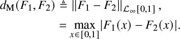
Definition 2.3. (Maximum and total distance) The maximum distance between functions F 1 and F 2 is defined as the  $\mathcal{L}_{\infty}\mbox{-}\text{norm}$ of F 1 and F 2 over $[0,1]$, that is,
 \begin{align*}
d_{\rm{M}}(F_1, F_2) & \triangleq \left\lVert F_1 - F_2\right\rVert_{\mathcal{L}_{\infty}[0,1]},\\
& = \max_{x \in [0,1]} \lvert F_1(x) - F_2(x) \rvert.
\end{align*}
\begin{align*}
d_{\rm{M}}(F_1, F_2) & \triangleq \left\lVert F_1 - F_2\right\rVert_{\mathcal{L}_{\infty}[0,1]},\\
& = \max_{x \in [0,1]} \lvert F_1(x) - F_2(x) \rvert.
\end{align*} The total distance between functions F 1 and F 2 is defined as the  $\mathcal{L}_{1}\mbox{-}\text{norm}$ of F 1 and F 2 over $[0,1]$, that is,
 \begin{align*}
d(F_1, F_2) & \triangleq \left\lVert F_1 - F_2\right\rVert_{\mathcal{L}_{1}[0,1]},\\
& = \int_0^1 \lvert F_1(x) - F_2(x) \rvert dx.
\end{align*}
\begin{align*}
d(F_1, F_2) & \triangleq \left\lVert F_1 - F_2\right\rVert_{\mathcal{L}_{1}[0,1]},\\
& = \int_0^1 \lvert F_1(x) - F_2(x) \rvert dx.
\end{align*}We mainly focus on the total distance and use the maximum distance as a secondary metric. As the maximum and total distance are designed to be applied to the polished functions, the exact value of the total distance and maximum distance of the linear/monotone cubic interpolation of the polished functions can be calculated.
3. Solutions and approximations
3.1. The Chebyshev–Markov (CM) inequalities
The authors [Reference Shohat and Tamarkin23] provide a method for obtaining  $\inf_{F\in \mathcal{F}_n} F(x_0)$ and $\sup_{F\in \mathcal{F}_n} F(x_0)$ for any $x_0 \in [0,1]$. The most important step of the method is the construction of a discrete distribution in $\mathcal{F}_n$, where the maximum possible mass is concentrated at x 0. The details of the method can be found in [Reference Markov14, Reference Shohat and Tamarkin23] and explicit expressions can be found in [Reference Wang and Haenggi28, Reference Zelen31]. The inequalities established by the infima and suprema in [Reference Wang and Haenggi28, Thm. 1] are also known as the CM inequalities. In contrast, the infima and suprema in [Reference Rácz, Tari and Telek20] are for distributions where the support can be an arbitrary Borel subset of $\mathbb{R}$. As a result, they are loose for distributions with support $[0,1]$.
Figure 1 shows two examples of the infima and suprema for different n. The convergence of the infima and suprema as n increases is apparent. The discontinuities of the derivatives in Figure 1 coincide with the roots of the orthogonal polynomials [Reference Wang and Haenggi28, Thm. 1]. For Figure 1(b),  $\underline{H}_{9} = 0$ indicates a discrete distribution. The infima and suprema get drastically closer from n = 8 to n = 10 because n = 10 is sufficient to characterize a discrete distribution with 5 jumps while n = 8 is not. In fact, the infima and suprema match almost everywhere (except at the jumps) for n = 10, but Figure 1(b) only reveals the mismatch at 0.5 and 0.8 since only 0.5 and 0.8 are jumps that fall in the sampling set $\mathcal{U}_{50}=\{i/50, \, i \in [50]_0\}$.
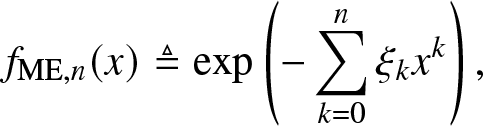
While all solutions to the THMP lie in the band defined by the infima and suprema, the converse does not necessarily hold. Figure 2 gives an example, where F lies in the band but is not a solution to the THMP. Its corresponding m 1 and m 2 are  $2/3$ and $1/2$, respectively, rather than $1/2$ and $1/3$ that define the band.
In the following subsections, we propose a method based on the Fourier–Chebyshev (FC) series and a CM method based on the average of the infima and suprema from the CM inequalities and compare them against the existing methods. We also improve and concretize some of the existing methods. {In particular, we provide a detailed discussion of the existing Fourier–Jacobi (FJ) approximations and fully develop the one mentioned in [Reference Shohat and Tamarkin23]. Besides, among all the discussed methods, the maximum entropy (ME) method by design yields solutions to the THMP, while the other methods by design obtain approximations of a solution to the THMP.

Figure 1. The infima and suprema from the CM inequalities for  $n = 4, 6, 8, 10$. x is discretized to $\mathcal{U}_{50} = \{i/50, \, i \in [50]_0\}$ a) $m_k = 1/(k+1),\quad k \in {[n]}_0$. b) $m_k = \frac{1}{5}( 8^{-k} + 3^{-k} + 2^{-k} + \left(\frac{3}{2}\right)^{-k} + \left(\frac{5}{4}\right)^{-k}),\quad k \in {[n]}_0$.
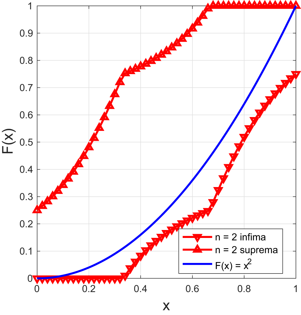
Figure 2. The infima and suprema from the CM inequalities for  $m_n = 1/(n+1)$ and $F(x) = x^2$.
3.2. Well-established methods
3.2.1. Binomial mixture (BM) method
A piecewise approximation of the cdf based on binomial mixturesFootnote 2 was proposed in [Reference Mnatsakanov and Ruymgaart18]. For any positive integer n, the approximationFootnote 3 by the BM method is defined as follows.
Definition 3.1. (Approximation by the BM method)
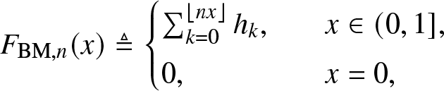 \begin{align}
{F}_{\mathrm{BM},n}(x) \triangleq
\begin{cases}
\sum_{k = 0}^{\lfloor nx \rfloor} h_k,&\quad x \in (0,1],\\
0, &\quad x = 0,
\end{cases}
\end{align}
\begin{align}
{F}_{\mathrm{BM},n}(x) \triangleq
\begin{cases}
\sum_{k = 0}^{\lfloor nx \rfloor} h_k,&\quad x \in (0,1],\\
0, &\quad x = 0,
\end{cases}
\end{align} where  $h_k = \sum_{i= k }^{n} \binom{n}{i} \binom{i}{k} (-1)^{i-k} m_i$.
Note that  $ {F}_{\mathrm{BM},n} \to F $ as $n \to \infty$ for each x at which F is continuous [Reference Mnatsakanov17, Reference Mnatsakanov and Ruymgaart18].
Let  $\hat{F}_{\mathrm{BM},n}$ denote the monotone cubic interpolation of ${{F}_{\mathrm{BM},n}}|_{\mathcal{U}_{n+1}}$ [Reference Haenggi6]. As shown in Figure 3, $ {F}_{\mathrm{BM},n} $ is piecewise constant, and for a continuous F, $\hat{F}_{\mathrm{BM},n}$ provides a better approximation than ${F}_{\mathrm{BM},n}$. Note that ${{F}_{\mathrm{BM},n}}$ is a solution to the THMP only when n = 1 and $\hat{F}_{\mathrm{BM},n}$ is not necessarily a solution for any positive integer n.
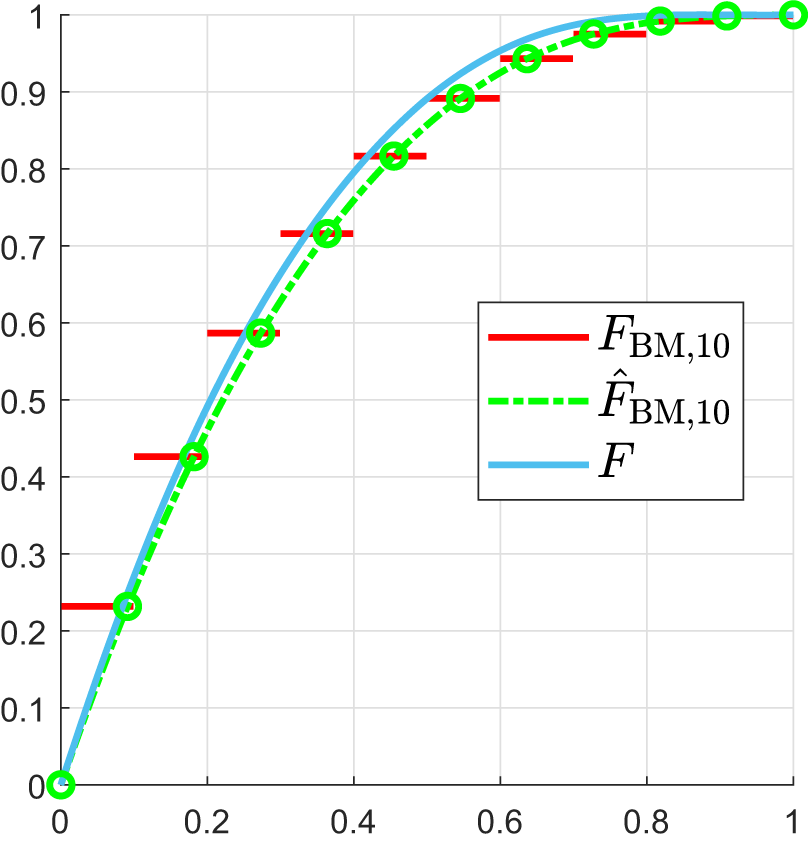
Figure 3.  $F_{\mathrm{BM},10}$, $\hat{F}_{\mathrm{BM},10}$ and F, where $\bar{F} = \exp(-\frac{x}{1-x}) (1-x)/ (1-\log(1-x))$. The $\circ$ denote ${F}_{\mathrm{BM},10}|_{\mathcal{U}_{11}}$.
3.2.2. ME method
The ME method [Reference Kapur12, Reference Mead and Papanicolaou16, Reference Tagliani25] is also widely used to solve the THMP. For any positive integer n, the solution by the ME method is defined as follows.
Definition 3.2. (Solution by the ME method)
 \begin{align}
f_{\mathrm{ME}, n}(x) \triangleq \exp\left(-\sum_{k = 0}^n \xi_k x^k\right),
\end{align}
\begin{align}
f_{\mathrm{ME}, n}(x) \triangleq \exp\left(-\sum_{k = 0}^n \xi_k x^k\right),
\end{align} where the coefficients  $\xi_k,i \in [n]_0$, are obtained by solving the equations
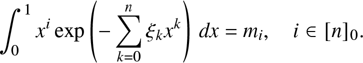 \begin{align}
\int_0^1 x^i \exp\left(-\sum_{k = 0}^n \xi_k x^k\right) \,dx = m_i, \quad i \in [n]_0.
\end{align}
\begin{align}
\int_0^1 x^i \exp\left(-\sum_{k = 0}^n \xi_k x^k\right) \,dx = m_i, \quad i \in [n]_0.
\end{align}A unique solution of (3.3) exists if and only if the Hankel determinants of the moment sequence are all positive. It can be obtained by minimizing the convex function [Reference Tagliani25]
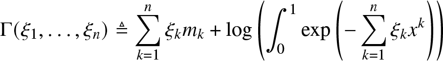 \begin{align}
\Gamma(\xi_1, \dots, \xi_n) \triangleq \sum_{k = 1}^n \xi_k m_k + \log\left( \int_{0}^{1} \exp\left(-\sum_{k =1}^n \xi_k x^k\right)\right)
\end{align}
\begin{align}
\Gamma(\xi_1, \dots, \xi_n) \triangleq \sum_{k = 1}^n \xi_k m_k + \log\left( \int_{0}^{1} \exp\left(-\sum_{k =1}^n \xi_k x^k\right)\right)
\end{align}and solving
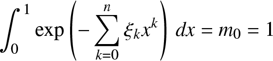 \begin{align}
\int_0^1 \exp\left(-\sum_{k = 0}^n \xi_k x^k\right) \,dx = m_0 = 1
\end{align}
\begin{align}
\int_0^1 \exp\left(-\sum_{k = 0}^n \xi_k x^k\right) \,dx = m_0 = 1
\end{align}for ξ 0. The corresponding cdf is given by
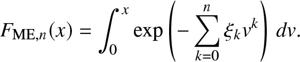 \begin{align}
F_{\mathrm{ME}, n}(x) = \int_0^x \exp\left(-\sum_{k = 0}^n \xi_k v^k\right)\, dv.
\end{align}
\begin{align}
F_{\mathrm{ME}, n}(x) = \int_0^x \exp\left(-\sum_{k = 0}^n \xi_k v^k\right)\, dv.
\end{align} Since (3.4) is convex, it can, in principle, be solved by standard techniques such as the interior point method. As the cdf given by (3.6) is a solution to the THMP, its error can be bounded by the infima and suprema from the CM inequalities, which, however, requires additional computation.  $F_{\mathrm{ME}, n} \to F$ in entropy and thus in $\mathcal{L}_1$ as $n \to \infty$ [Reference Tagliani25]. But due to ill-conditioning of the Hankel matrices [Reference Inverardi, Pontuale, Petri and Tagliani10], the ME method becomes impractical when the number of given moments is large, as solving (3.4) may not be feasible.
3.3. Improvements and concretization of existing methods
3.3.1. Gil–Pelaez (GP) method
The main part of this study focuses on the HMP and THMP, which are based on integer moments. However, for the purpose of performance evaluation in Section 4.5, here we also consider the reconstruction problem involving complex moments. By the Gil-Pelaez (GP) theorem [Reference Gil-Pelaez3], F at which F is continuousFootnote 4 can be obtained from the imaginary moments by
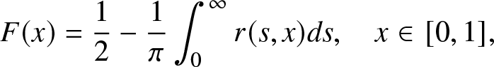 \begin{align}
{F} (x) & = \frac{1}{2} - \frac{1}{\pi} \int_0^\infty r(s,x) ds , \quad x \in [0,1],
\end{align}
\begin{align}
{F} (x) & = \frac{1}{2} - \frac{1}{\pi} \int_0^\infty r(s,x) ds , \quad x \in [0,1],
\end{align} where  $r(s,x) \triangleq {\Im{(e^{-js\log x} m_{js})}}/{s}$, $j \triangleq \sqrt{-1}$, and $\Im(z)$ is the imaginary part of the complex number z.
Since the integral in (3.7) cannot be analytically calculated, only numerical approximations can be obtained. An accurate evaluation is exacerbated by the facts that the integration interval is infinite and that the integrand may diverge at 0. We define the approximate value obtained through the trapezoidal rule as follows.
Definition 3.3. (Approximation by the GP method)
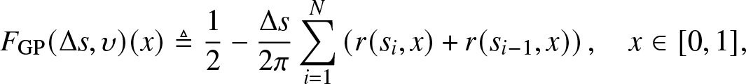 \begin{align}
{F}_{\rm{GP}}(\Delta s,\upsilon )(x) \triangleq
\frac{1}{2} - \frac{\Delta s}{2\pi} \sum_{i = 1}^{N} \left ( r(s_i,x) + r(s_{i-1},x) \right ), \quad x \in [0,1],
\end{align}
\begin{align}
{F}_{\rm{GP}}(\Delta s,\upsilon )(x) \triangleq
\frac{1}{2} - \frac{\Delta s}{2\pi} \sum_{i = 1}^{N} \left ( r(s_i,x) + r(s_{i-1},x) \right ), \quad x \in [0,1],
\end{align} where  $N \triangleq \lfloor\frac{\upsilon }{\Delta s}\rfloor$ and $s_i \triangleq i \Delta s$.
Note that as  $\Delta s \to 0$ and $\upsilon \to \infty$, $ {F}_{\rm{GP}},{\Delta s,\upsilon } \to {F} $ for each x at which F is continuous.
We evaluate  ${F}_{\rm{GP}}(\Delta s,\upsilon )$ over the set ${\mathcal{U}_{100}}$ for different $\Delta s$ and υ. Figure 4 shows the average of the total and maximum distance of F and polished $\hat{F}_{\rm{GP}}(\Delta s,\upsilon )$ as the step size $\Delta s$ and upper integration limit υ change. As the step size $\Delta s $ decreases to 0.1 and as the upper integration limit υ increases to $1,000$, the average of the total distance decreases to <10−3, which indicates that the approximate cdf obtained by numerically evaluating the integral of GP method is very close to the exact cdf and thus can be used as a reference. Both the integration upper limit and step size are critical in evaluating the integral. A general rule for selecting the upper integration limit is to examine the magnitude of mjs. For example, if $|m_{js}| \leq 1/s$, the error resulting from fixing the upper integration limit at $1,000$ is $\int_{1,000}^{\infty} r(s,x) ds \lt \int_{1,000}^{\infty} 1/s^2 ds = 10^{-3}$. However, it is not always possible to determine the rate of decay of the magnitude of the imaginary moments with only numerical values. So it is difficult to come up with a universal rule for the integration range that is suitable for all moment sequences.
For the GP method, we propose a dynamic way to adjust the values of the upper limit and step size. We start at  $F_{\rm{GP}(0.1, 1,000)}$. If the cdf determined by the previous selections exceeds $[0,1]$, we decrease the step size to $1/3$ of the previous one and increase the upper limit to 3 times the previous one and then recalculate the cdf. We repeat this process until the range of the cdf is in $[0,1]$. In some cases, the updated step size and upper limit may cause memory problems. The averaging process described in Section 4.5, we discard those cases if we detect that the required memory is larger than the available memory.
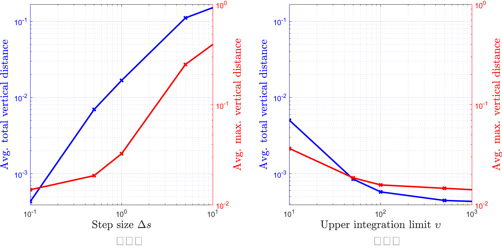
Figure 4. Average of the total and maximum distances between F and polished  $\hat{F}_{\rm{GP}}(\Delta s,\upsilon )$ which are averaged over 100 randomly generated beta mixtures as described in Section 4.4 (a) $\upsilon = 1,000$ (b) $\Delta s = 0.1$.
3.3.2. FJ method
Equipped with a complete orthogonal system on  $[0,1]$, denoted as $\left(T_k(x)\right)_{k = 0}^{\infty}$, we can expand a function l defined on $[0,1]$ to a generalized Fourier series as [Reference Szegö24]
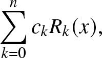
 \begin{align}
l(x) = \sum_{k = 0}^{\infty} c_k T_k (x).
\end{align}
\begin{align}
l(x) = \sum_{k = 0}^{\infty} c_k T_k (x).
\end{align} The Jacobi polynomials  $P_n^{(\alpha, \beta)}$ are such a class of orthogonal polynomials defined on $[-1,1]$. They are orthogonal w.r.t. the weight function $\omega^{(\alpha, \beta)} (x) \triangleq (1-x)^\alpha (x+1)^{\beta}$ [Reference Szegö24], that is,
 \begin{align}
\int_{-1}^{1} \omega^{(\alpha, \beta)} (x) P_n^{(\alpha, \beta)} (x)P_m^{(\alpha, \beta)} (x) \,dx
= \frac{2^{\alpha + \beta +1}
\left(n+1\right)^{(\beta)}
\delta_{mn}
}{(2n+\alpha + \beta +1)
\left(n+\alpha+1\right)^{(\beta)}} ,
\end{align}
\begin{align}
\int_{-1}^{1} \omega^{(\alpha, \beta)} (x) P_n^{(\alpha, \beta)} (x)P_m^{(\alpha, \beta)} (x) \,dx
= \frac{2^{\alpha + \beta +1}
\left(n+1\right)^{(\beta)}
\delta_{mn}
}{(2n+\alpha + \beta +1)
\left(n+\alpha+1\right)^{(\beta)}} ,
\end{align} where δmn is the Kronecker delta function, and  $a^{(b)}\triangleq{\frac {\Gamma (a+b)}{\Gamma (a)}}$ is the Pochhammer function. For $\alpha = \beta = 0$, they are the Legendre polynomials; for $\alpha = \beta = \pm 1/2$, they are the Chebyshev polynomials. The shifted Jacobi polynomials
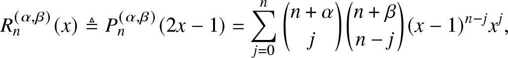 \begin{align}
R_n^{(\alpha, \beta)} (x) &\triangleq P_n^{(\alpha, \beta)} (2x-1) = \sum_{j = 0}^{n} \binom{n + \alpha}{j} \binom{n+\beta}{n - j} (x-1)^{n-j} x^j,
\end{align}
\begin{align}
R_n^{(\alpha, \beta)} (x) &\triangleq P_n^{(\alpha, \beta)} (2x-1) = \sum_{j = 0}^{n} \binom{n + \alpha}{j} \binom{n+\beta}{n - j} (x-1)^{n-j} x^j,
\end{align} are defined on  $[0,1]$. Letting
  $\eta_n^{(\alpha, \beta)}\triangleq \frac{\left(n+1\right)^{(\beta)}
}{(2n+\alpha + \beta +1)
\left(n+\alpha+1\right)^{(\beta)}
}$, the corresponding orthogonality condition w.r.t. the weight function
$\eta_n^{(\alpha, \beta)}\triangleq \frac{\left(n+1\right)^{(\beta)}
}{(2n+\alpha + \beta +1)
\left(n+\alpha+1\right)^{(\beta)}
}$, the corresponding orthogonality condition w.r.t. the weight function  $w^{(\alpha, \beta)}(x) \triangleq (1-x)^{\alpha} x^\beta$ is
 \begin{align}
\int_{0}^{1} w^{(\alpha, \beta)}(x) R_n^{(\alpha, \beta)} (x)R_m^{(\alpha, \beta)} (x) \,dx= \eta_n^{(\alpha, \beta)}\delta_{mn}.
\end{align}
\begin{align}
\int_{0}^{1} w^{(\alpha, \beta)}(x) R_n^{(\alpha, \beta)} (x)R_m^{(\alpha, \beta)} (x) \,dx= \eta_n^{(\alpha, \beta)}\delta_{mn}.
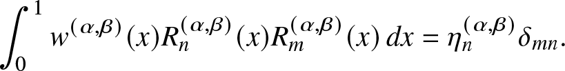
\end{align}When applying the FJ series to solve (2.1), the usual approach is to expand the target function (cdf or pdf) as
 \begin{align}
w^{(\alpha, \beta)}(x) \sum_{k = 0}^{\infty} c_k R_k^{(\alpha, \beta)} (x),
\end{align}
\begin{align}
w^{(\alpha, \beta)}(x) \sum_{k = 0}^{\infty} c_k R_k^{(\alpha, \beta)} (x),
\end{align} so that the moments can be utilized in the orthogonality conditions. However, an approximation obtained by the n-th partial sum of the expansion is usually not a solution to the THMP, for two reasons. First, the remaining Fourier coefficients,  $c_m and m \gt n$, may not all be zero. Second, the approximations may not preserve the properties of probability distributions.
Convergence is a major concern when approximating a function by an FJ series. While no conditions are known that are both sufficient and necessary, there exist sufficient conditions and there exist necessary conditions, both of which depend on the values of  $\alpha, \beta$, and the properties of the approximated functions [Reference Li13, Reference Pollard19]. For the THMP, a basic question is whether $\alpha, \beta$ should depend on the moment sequence or not and whether to approximate pdfs or cdfs. In the following, we will discuss in detail three different ways which have been proposed in [Reference Guruacharya and Hossain4, Reference Schoenberg22, Reference Shohat and Tamarkin23], respectively. In particular, [Reference Guruacharya and Hossain4] set $\alpha, \beta$ depending on the moment sequences and only approximate pdfs. In the other two ways, cdfs and pdfs are approximated, respectively, and both fix $\alpha=\beta = 0$ [Reference Schoenberg22, Reference Shohat and Tamarkin23].
In the FJ method based on the FJ series [Reference Guruacharya and Hossain4],  $\alpha, \beta$ are chosen such that the first two Fourier coefficients c 1 and c 2 are zero, that is, $\alpha+ 1 = (m_1- m_2) (1-m_1)/{(m_2 - m_1^2)}$ and $\beta + 1 = {(\alpha + 1) m_1}/{(1 - m_1)}$. For any positive integer n, the approximation by the FJ method is defined as follows.
Definition 3.4. (Approximation by the FJ method [Reference Guruacharya and Hossain4])
 \begin{align}
f_{\mathrm{FJ},n}(x) \triangleq w^{(\alpha, \beta)} (x) \sum_{k = 0}^n c_k R_k^{(\alpha, \beta)} (x),
\end{align}
\begin{align}
f_{\mathrm{FJ},n}(x) \triangleq w^{(\alpha, \beta)} (x) \sum_{k = 0}^n c_k R_k^{(\alpha, \beta)} (x),
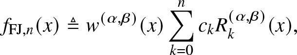
\end{align}where, by the orthogonality condition,
 \begin{align}
c_m
= & \frac{1}{\eta_m^{(\alpha, \beta)}} \sum_{j = 0}^m \binom{m+\alpha}{j} \binom{m+\beta}{m-j} \sum_{k = 0}^{m-j} \binom{m-j}{k} (-1)^k m_{m-k}.
\end{align}
\begin{align}
c_m
= & \frac{1}{\eta_m^{(\alpha, \beta)}} \sum_{j = 0}^m \binom{m+\alpha}{j} \binom{m+\beta}{m-j} \sum_{k = 0}^{m-j} \binom{m-j}{k} (-1)^k m_{m-k}.
\end{align}The corresponding cdf is
 \begin{align}
F_{\mathrm{FJ},n}(x)
= \frac{
\left(\alpha+1\right)^{(\beta+1)}
}{
\Gamma( \beta+1) } \int_{0}^{x} w^{(\alpha, \beta)} (t) dt
- \sum_{k = 1}^n \frac{c_k}{k} w^{(\alpha+1, \beta+1)}(x) R_{k-1}^{(\alpha+1, \beta+1)} (x).
\end{align}
\begin{align}
F_{\mathrm{FJ},n}(x)
= \frac{
\left(\alpha+1\right)^{(\beta+1)}
}{
\Gamma( \beta+1) } \int_{0}^{x} w^{(\alpha, \beta)} (t) dt
- \sum_{k = 1}^n \frac{c_k}{k} w^{(\alpha+1, \beta+1)}(x) R_{k-1}^{(\alpha+1, \beta+1)} (x).
\end{align}  $F_{\mathrm{FJ},1} = F_{\mathrm{FJ},2}$ correspond to the beta approximation [Reference Haenggi5], where m 1 and m 2 are matched with the corresponding moments of a beta distribution.
There are three drawbacks of the FJ method. First, as  $\alpha and \beta$ vary significantly for different moment sequences, the convergence properties of the FJ method vary strongly as well. So it is impossible to give a conclusive answer to whether such approximations converge or not. It is a critical shortcoming of the FJ method that it only converges in some cases. Second, as α and β are generally not zero, the approximate pdf is always 0 or $\infty$ at x = 0 and x = 1, which holds only for a limited class of pdfs. Last but not least, it is possible that, as a functional approximation, the FJ method leads to non-monotonicity in the approximate cdf. We address this by applying the tweaking mapping in Definition 2.2 to $F_{\mathrm{FJ},n} |_{\mathcal{U}_n}$.
3.3.3. Fourier–Legendre (FL) method
The authors [Reference Schoenberg22, Reference Shohat and Tamarkin23] suggest fixing  $\alpha = \beta = 0$ in advance. The resulting polynomials are Legendre polynomials with weight function 1. To expand a function l by the FL series, a necessary condition for convergence is that the integral $\int_0^1 l(x) (1-x)^{-1/4} x^{-1/4} \, dx$ exists [Reference Szegö24]. Furthermore, if $l \in \mathcal{L}^p$ with $p \gt 4/3$, the FL series converges pointwise [Reference Pollard19]. There still remains the question of whether we should approximate the pdf or the cdf. In the following, we will discuss the two cases. The two have been discussed separately in [Reference Schoenberg22, Reference Shohat and Tamarkin23], but the concrete expressions of the coefficients are missing. Besides, to the best of our knowledge, their convergence properties have not been compared.
We denote the corresponding pdf of F as f and  $R_k^{(0,0)}$ as Rk.
Approximating the pdf [Reference Schoenberg22] The n-th partial sum of the FL expansion of the pdf is
 \begin{align}
\sum_{k = 0}^{n} c_k R_k(x),
\end{align}
\begin{align}
\sum_{k = 0}^{n} c_k R_k(x),
\end{align}where, by the orthogonality condition,
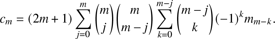 \begin{align}
c_m
&= (2m+1) \sum_{j = 0}^m \binom{m}{j} \binom{m}{m - j} \sum_{k =0}^{m-j} \binom{m-j}{k}(-1)^{k} m_{m-k}.
\end{align}
\begin{align}
c_m
&= (2m+1) \sum_{j = 0}^m \binom{m}{j} \binom{m}{m - j} \sum_{k =0}^{m-j} \binom{m-j}{k}(-1)^{k} m_{m-k}.
\end{align} It does not always hold that  $f \in \mathcal{L}^p[0,1]$ with $p \gt 4/3$. Thus, the series does not converge for some f, for example, the pdf of $\mathrm{Beta} (1, \beta)$ with $0 \lt \beta \leq 1/4$ or $\mathrm{Beta} (\alpha, 1)$ with $0 \lt \alpha \leq 1/4$. Worse yet, it is possible that the FL series diverges everywhere, for example, the FL series of $f(x) = (1-x)^{-3/4}/4$.
So similar to the FJ method, approximating the pdf does not guarantee convergence.
Approximating the cdf [Reference Shohat and Tamarkin23] The n-th partial sum of the FL expansion of the cdf is
 \begin{align}
\sum_{k = 0}^{n} c_k R_k(x),
\end{align}
\begin{align}
\sum_{k = 0}^{n} c_k R_k(x),
\end{align}where, by the orthogonality condition,
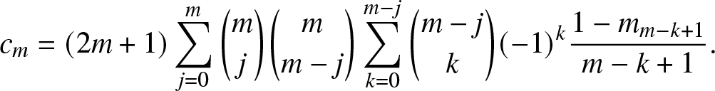 \begin{align}
c_m
&= (2m+1) \sum_{j = 0}^m \binom{m}{j} \binom{m}{m - j} \sum_{k =0}^{m-j} \binom{m-j}{k}(-1)^{k}
\frac{1 - m_{m-k+1}}{m-k+1}.
\end{align}
\begin{align}
c_m
&= (2m+1) \sum_{j = 0}^m \binom{m}{j} \binom{m}{m - j} \sum_{k =0}^{m-j} \binom{m-j}{k}(-1)^{k}
\frac{1 - m_{m-k+1}}{m-k+1}.
\end{align}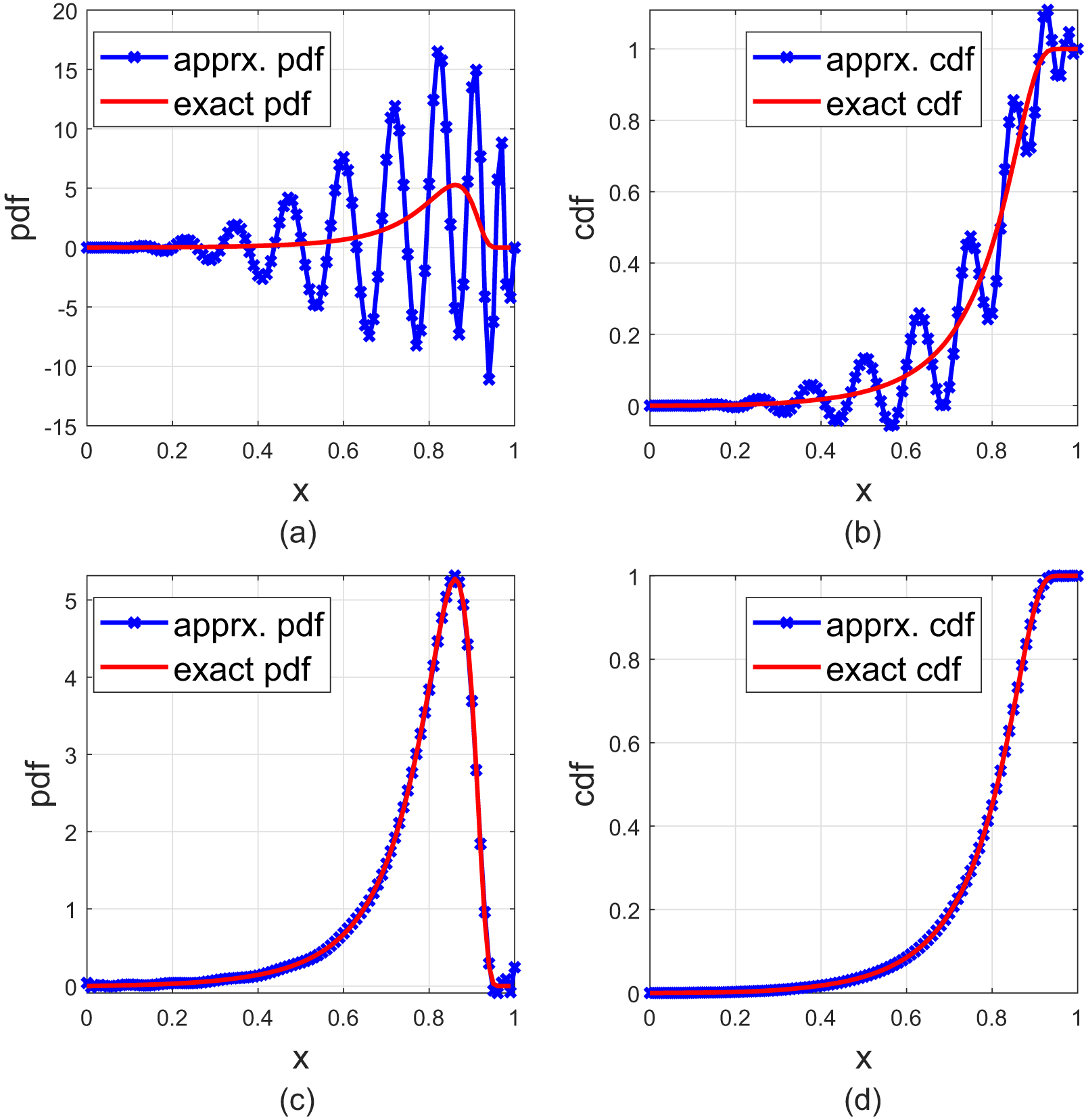
Figure 5. The upper two plots are for the FJ method [Reference Guruacharya and Hossain4] with n = 20, and the lower two plots are for the FL series with n = 20. The cdf is given in (3.21).
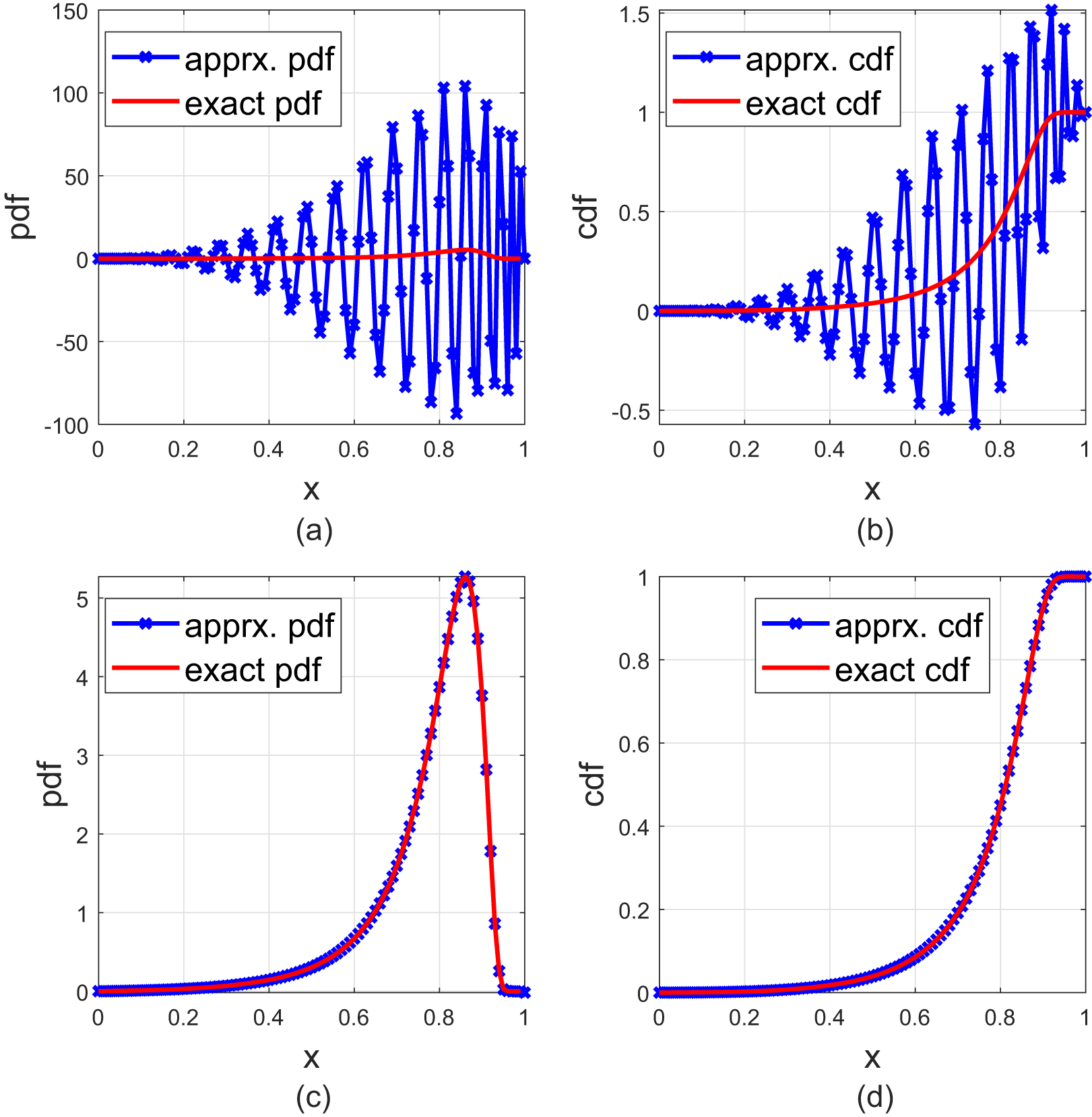
Figure 6. The upper two plots are for FJ method [Reference Guruacharya and Hossain4] with n = 40, and the lower two plots are for the FL series with n = 40. The cdf is given in (3.21).
Since F is always bounded and thus  $F \in \mathcal{L}^p[0,1]$ for any $p \geq 1$, pointwise convergence holds [Reference Pollard19]. Comparisons of the FJ method and approximating the pdf via the FL series In Figures 5 and 6, where
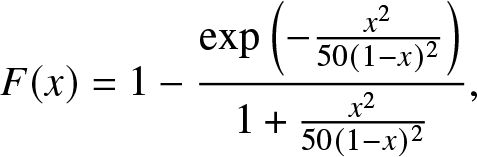 \begin{align}
{F}(x) = 1- \frac{\exp\left(- \frac{x^2}{50(1-x)^2}\right) }{ 1 + \frac{x^2}{50(1-x)^2} },
\end{align}
\begin{align}
{F}(x) = 1- \frac{\exp\left(- \frac{x^2}{50(1-x)^2}\right) }{ 1 + \frac{x^2}{50(1-x)^2} },
\end{align}we approximate the pdf by the FJ method and by the FL series. We observe that in both cases, the FL approximations are much better than the FJ ones. Also, the FL approximations do better as n increases.
Comparisons of approximating the pdf and cdf by the FL series Figure 7 shows the approximate cdfs by using the FL series to approximate the pdf and then integrate and directly approximate the cdf, respectively. We observe that approximating cdfs leads to a more accurate result.
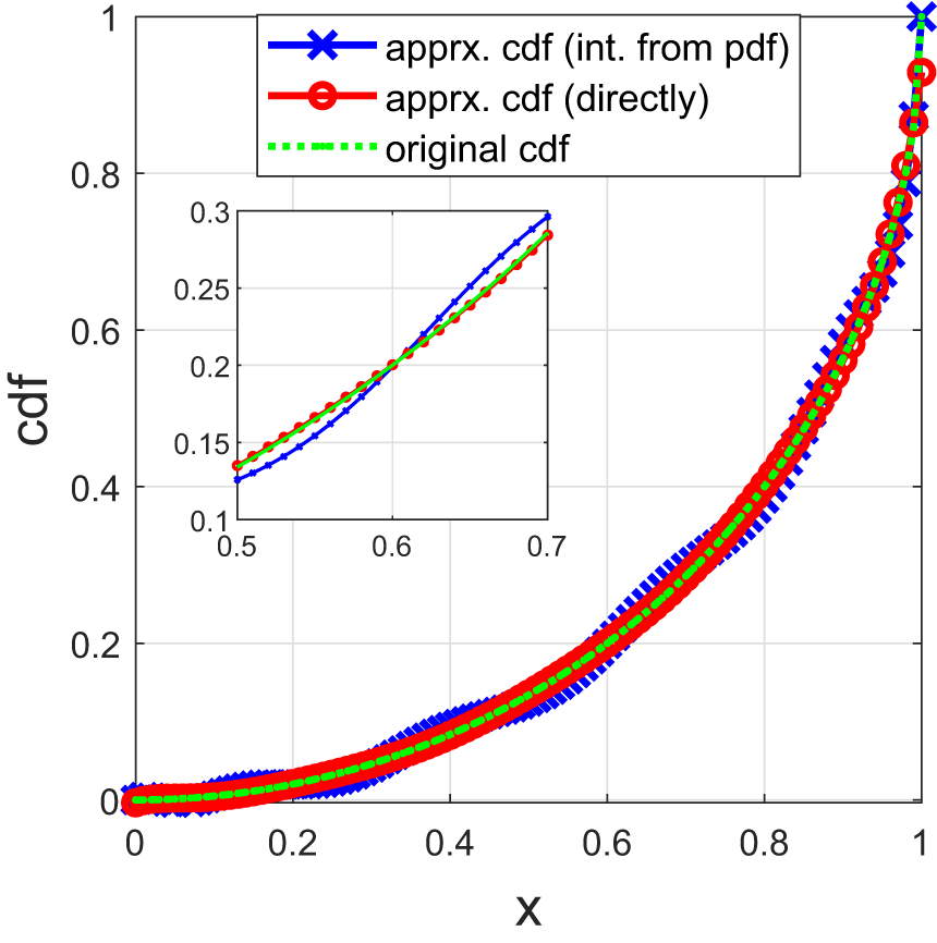
Figure 7. Reconstructed cdfs of  $F(x) = 1 - \sqrt{1-x^2}$ based on 10 moments. The blue curve shows the reconstructed cdf from approximating the pdf, the red curve shows the reconstructed cdf from approximating the cdf, and the green curve shows F.
Considering that a pdf may not be in  $\mathcal{L}^p[0,1]$ with $p \gt 4/3$ but a cdf always is, in the following, we use the FL series to approximate the cdf and call it the FL method. For any positive integer n, the approximation by the FL method is defined as follows.
Definition 3.5. (Approximation by the FL method)
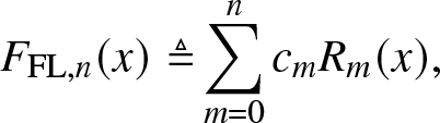 \begin{align}
F_{\mathrm{FL},n}(x) \triangleq&
\sum_{m = 0}^{n} c_m R_m(x),
\end{align}
\begin{align}
F_{\mathrm{FL},n}(x) \triangleq&
\sum_{m = 0}^{n} c_m R_m(x),
\end{align} where  $c_m, \, m \in [n]_0$, are given by (3.20).
Since it is a functional approximation, we apply the tweaking mapping in Definition 2.2 to  $F_{\mathrm{FL},n-1}|_{\mathcal{U}_{n}}$.
3.4. New methods
3.4.1. FC method
Similar to the idea in Section 3.3.3 that we fix α and β in advance, here we use the FC series for approximation, that is, we set  $\alpha = \beta = -1/2$. To guarantee convergence, similar to the FL method, we also focus on approximating the cdf and call it the FC method. For any positive integer n, the approximation by the FC method is defined as follows.
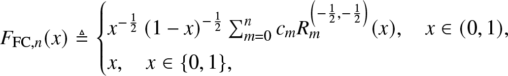
Definition 3.6. (Approximation by the FC method)
 \begin{align}
F_{\mathrm{FC}, n} (x)\triangleq
\begin{cases}
x^{-\frac{1}{2}}\left(1-x\right)^{-\frac{1}{2}} \sum_{m = 0}^n c_m R_m^{\left(-\frac{1}{2}, -\frac{1}{2} \right)}(x), \quad x \in (0,1),\\
x, \quad x \in \{0,1\},
\end{cases}
\end{align}
\begin{align}
F_{\mathrm{FC}, n} (x)\triangleq
\begin{cases}
x^{-\frac{1}{2}}\left(1-x\right)^{-\frac{1}{2}} \sum_{m = 0}^n c_m R_m^{\left(-\frac{1}{2}, -\frac{1}{2} \right)}(x), \quad x \in (0,1),\\
x, \quad x \in \{0,1\},
\end{cases}
\end{align}where, by the orthogonality condition,
 \begin{align}
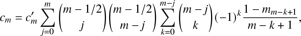
c_m
&= c'_m \sum_{j = 0}^m \binom{m-1/2}{j} \binom{m-1/2}{m - j} \sum_{k =0}^{m-j} \binom{m-j}{k}(-1)^{k}
\frac{1 - m_{m-k+1}}{m-k+1},
\end{align}
\begin{align}
c_m
&= c'_m \sum_{j = 0}^m \binom{m-1/2}{j} \binom{m-1/2}{m - j} \sum_{k =0}^{m-j} \binom{m-j}{k}(-1)^{k}
\frac{1 - m_{m-k+1}}{m-k+1},
\end{align}  $c'_0 = 1/\pi$ and $c'_m = 2 \left( \frac{\Gamma(m+1)}{\Gamma(m+1/2)}\right)^2$, $m \in [n]$.
As F and  $x^{\frac{1}{2}}\left(1-x\right)^{\frac{1}{2}} $ are of bounded variation, the function $F x^{\frac{1}{2}}\left(1-x\right)^{\frac{1}{2}}$ approximated by the FC series has bounded variation, thus uniform convergence holds [Reference Mason and Handscomb15]. To preserve the properties of probability distributions, we apply the tweaking mapping in Definition 2.2 to $F_{\mathrm{FC}, n-1}|_{\mathcal{U}_{n}}$.
3.4.2. CM method
As the CM inequalities provide the infima and suprema at the points of interest among the family of solutions given a sequence of length n, it is important to analyze the distribution of the unique solution given the sequence of an infinite length. Here, we explore this distribution at point x = 0.5 by simulating the distribution of infima and suprema of a sequence of length 8 within the initial ranges define by the infima and suprema given the first three elements in the sequence. For example, let  $\underline{F}_3$ and $\bar{F}_3$ denote the infimum and supremum defined by the CM inequalities at point 0.5 given a sequence $(m_1, m_2, m_3)$, and let $\underline{F}_8$ and $\bar{F}_8$ denote the infimum and supremum defined by the CM inequalities at point 0.5 given a sequence $(m_1, m_2, m_3, m_4, m_5, m_6, m_7, m_8)$. We focus on the relative position of $\underline{F}_8$ and $\bar{F}_8$ within the range defined by $\underline{F}_3$ and $\bar{F}_3$, that is, the normalized $x = \left(\underline{F}_8 - \underline{F}_3 \right)/\left(\bar{F}_3- \underline{F}_3\right)$ and $x = \left(\bar{F}_8 - \underline{F}_3 \right)/\left(\bar{F}_3 - \underline{F}_3\right)$. The average is calculated as $\left(\bar{F}_8+ \underline{F}_8 \right)/2$.
Algorithm 1. Algorithm for random moment sequences by canonical moments
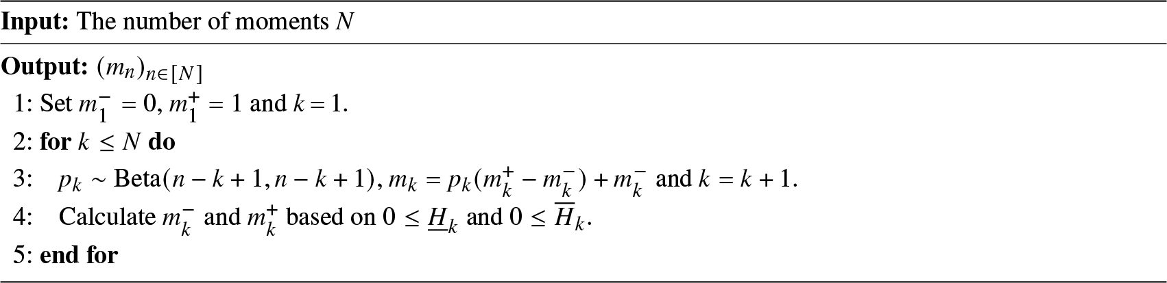
Figure 8 and Figure 9 show the normalized histograms with beta distribution fit. From both of them, we can observe that there is symmetry between the distribution of the infima and suprema, and their average is concentrated in the middle. In particular, in Figure 9, we observe that its average concentrates more in the middle compared to Figure 8, since the first three moments come from the uniform distribution. This finding indicates that the unique solution of a moment sequence of infinite length is likely to be centered within the infima and suprema defined by its truncated sequence. Therefore, it is sensible to consider their average as an approximation to a solution to the THMP and we call it the CM method. For any positive integer n, the approximation by the CM method is defined as follows.
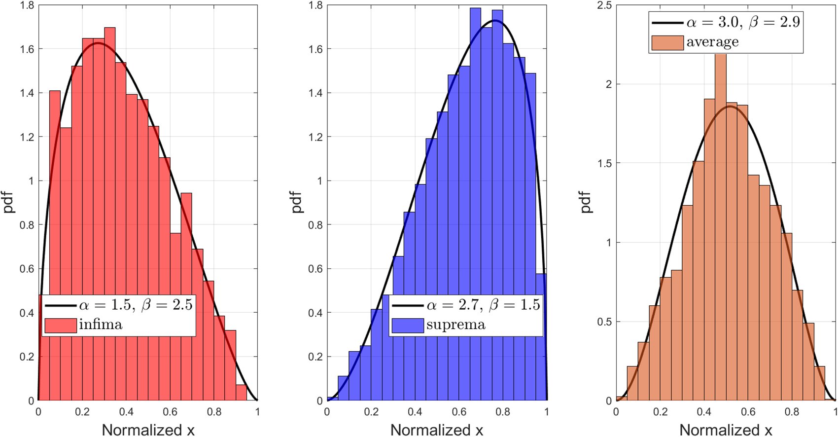
Figure 8. The normalized histogram of infima, suprema, and average and the corresponding beta distribution fit for 50 realizations of moment sequences of length 3 generated by Algorithm 1, each of which has been further extended 50 times to length 8 by Algorithm 1. The two parameters of the beta distribution fit are based on the first two empirical moments.
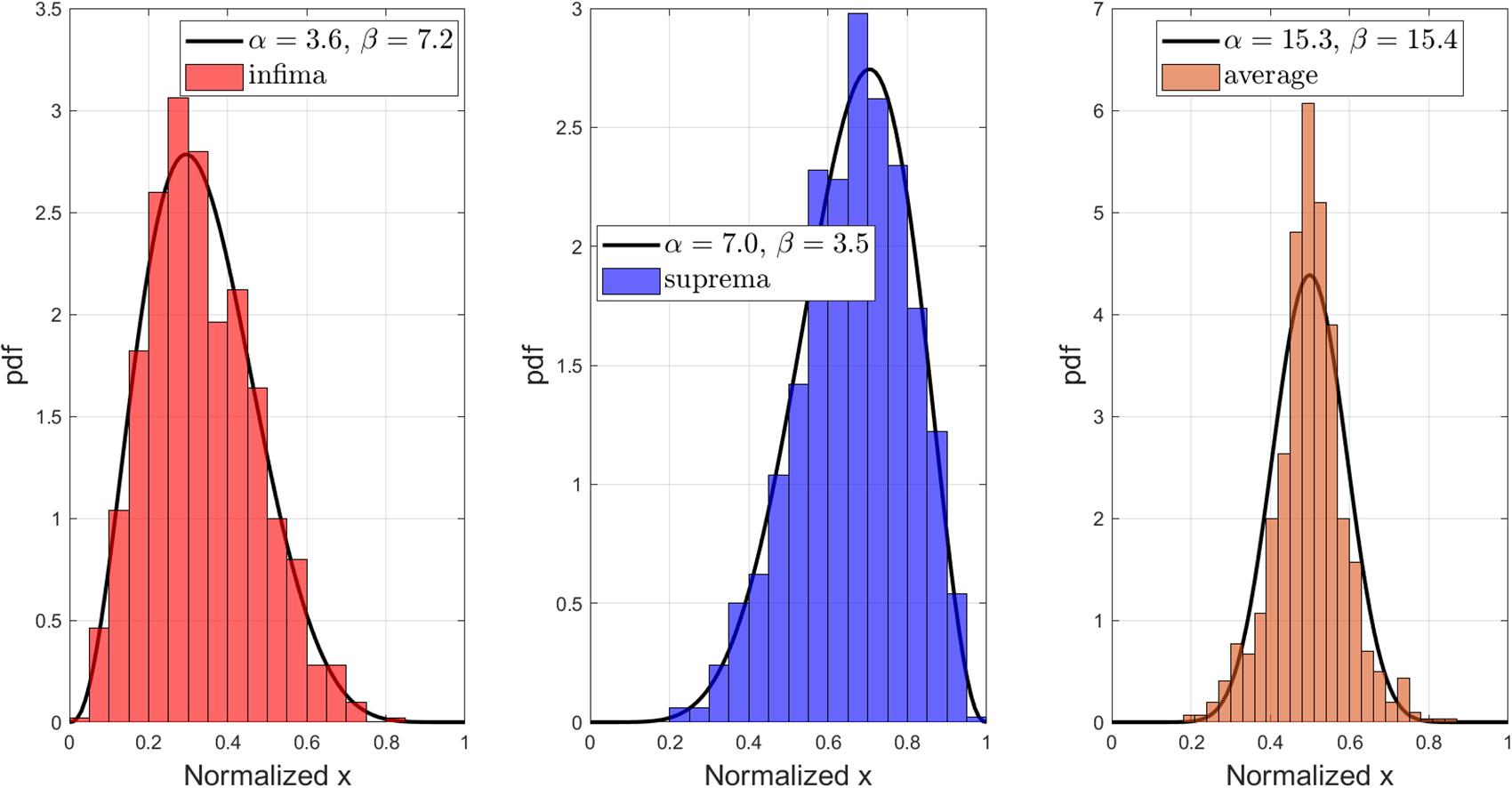
Figure 9. The normalized histogram of infima, suprema, and average and the corresponding beta distribution fit for  $1,000$ realizations of moment sequences of length 8 generated by Algorithm 1, each of which has the same first 3 elements as $(1/2, 1/3, 1/4)$. The two parameters of the beta distribution fit are based on the first two empirical moments.
Definition 3.7. (Approximation by the CM method)
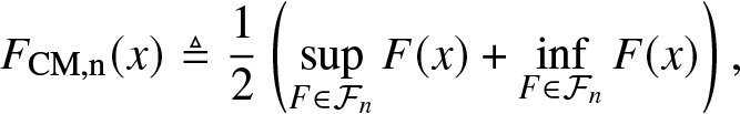 \begin{align}
F_{\rm{CM},n}(x) \triangleq \frac{1}{2} \left(\sup_{F\in \mathcal{F}_n} F(x) + \inf_{F\in \mathcal{F}_n} F(x) \right),
\end{align}
\begin{align}
F_{\rm{CM},n}(x) \triangleq \frac{1}{2} \left(\sup_{F\in \mathcal{F}_n} F(x) + \inf_{F\in \mathcal{F}_n} F(x) \right),
\end{align} where  $\sup_{F\in \mathcal{F}_n} F(x) $ and $\inf_{F\in \mathcal{F}_n} F(x)$ are given by the CM inequalities.
From Figure 10, we observe that the average is very close to the original cdf, and it is slightly better than the beta approximation. It is worth noting that by averaging, the error can be bounded: For all  $x \in [0,1]$ and for all $F \in \mathcal{F}_n$,
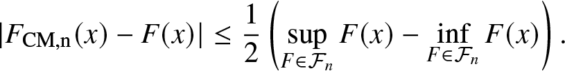 \begin{align}
|F_{\rm{CM},n}(x) - F(x) | \leq \frac{1}{2} \left(\sup_{F\in \mathcal{F}_n} F(x) - \inf_{F\in \mathcal{F}_n} F(x) \right).
\end{align}
\begin{align}
|F_{\rm{CM},n}(x) - F(x) | \leq \frac{1}{2} \left(\sup_{F\in \mathcal{F}_n} F(x) - \inf_{F\in \mathcal{F}_n} F(x) \right).
\end{align} Although  $F_{\rm{CM},n}$ lies within the band defined by the infima and suprema from the CM inequalities, it is not necessarily one of the infinitely many solutions to the THMP. Moreover, it is almost never a solution. For example, $F_{\rm{CM},1}$ is a solution only when $m_1 = 1/2$.
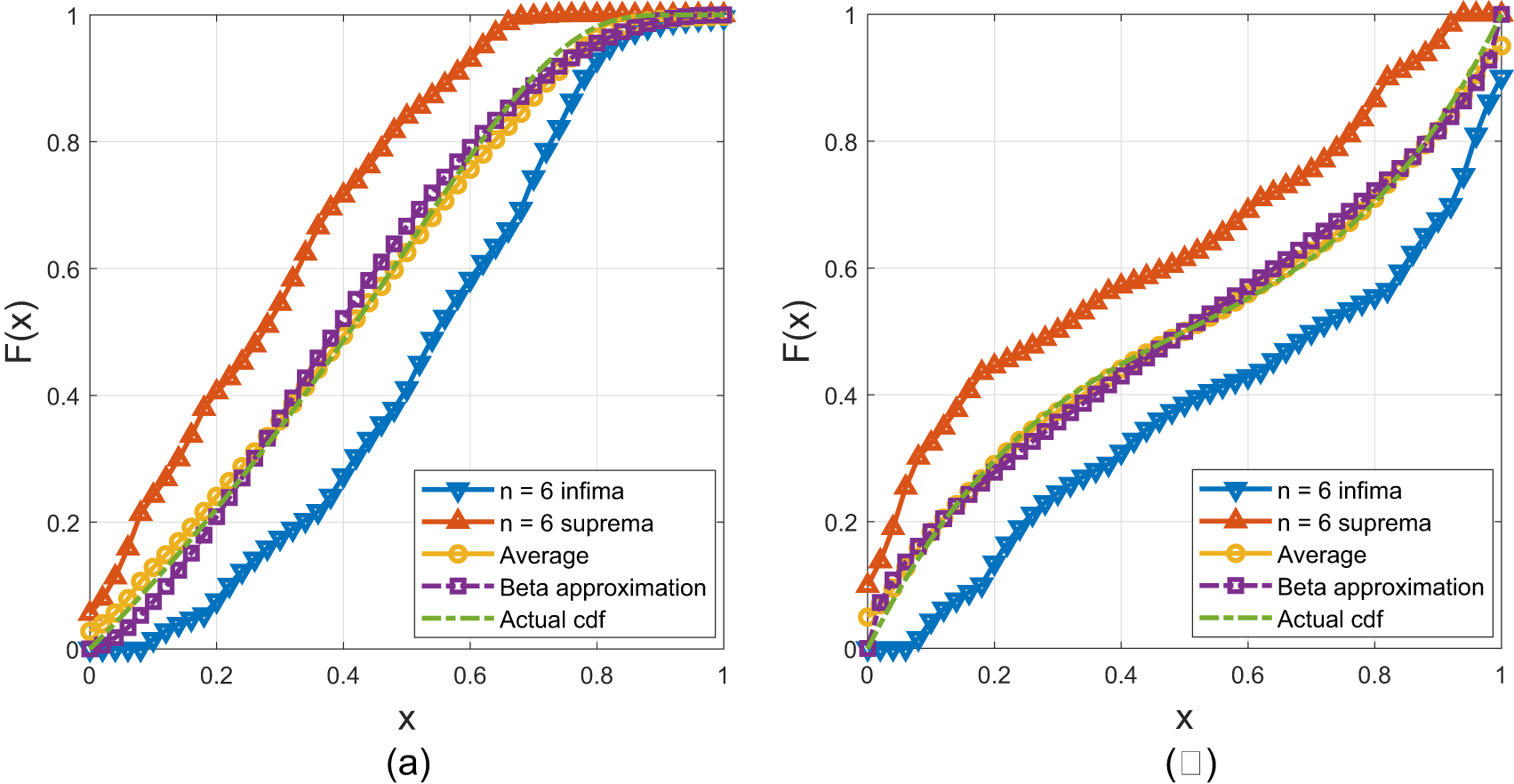
Figure 10. The infima and suprema from the CM inequalities, their average, and the beta approximation given  $(m_k)_{k = 0}^6$ a) $F(x) =\exp(-x/(1-x))$. The total difference is 0.015 between $\hat{F}_{\rm{CM},6}$ and the actual cdf and 0.019 for the beta approximation. b) $F(x) = \frac{1}{2}\int_0^1 (x^{10}(1-x) + x(1-x)^{10}) \, dx$. The total difference is 0.0199 between $\hat{F}_{\rm{CM},6}$ and the actual cdf and 0.0451 for the beta approximation.
3.5. The methods as linear transforms
The calculation of the coefficients in the BM method and methods based on the FJ series, such as the FL and FC method, where the coefficients α and β are fixed, can be written as linear transforms of the given sequence, with the transform matrix being fixed for each method. This can be pre-computed offline, accelerating the calculation.Footnote 5 We discuss the BM and FL method in detail.
As we recall, for the BM method [Reference Haenggi6], we can write  $\mathbf{h} \triangleq \left(h_l\right)_{l = 0}^n$ as a linear transform of $\mathbf{m} \triangleq (m_l)_{l = 0}^{n}$, that is,
 \begin{align}
\mathbf{h} = \mathbf{A} \mathbf{m},
\end{align}
\begin{align}
\mathbf{h} = \mathbf{A} \mathbf{m},
\end{align} where m and h are column vectors and the transform matrix  $\mathbf{A} \in \mathbb{Z}^{(n+1)\times(n+1)}$ is given by
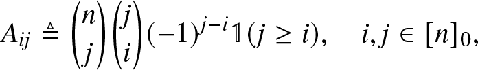 \begin{align}
A_{ij} \triangleq \binom{n}{j} \binom{j}{i} (-1)^{j-i} \mathbb{1}{(j \geq i)}, \quad i,j \in [n]_0,
\end{align}
\begin{align}
A_{ij} \triangleq \binom{n}{j} \binom{j}{i} (-1)^{j-i} \mathbb{1}{(j \geq i)}, \quad i,j \in [n]_0,
\end{align} where  $\mathbb{1}$ is the indicator function. The transform matrix needs to be calculated only once for each n, which can be done offline. The matrix-vector multiplication requires $\frac{(n+1)(n+2)}{2}$ multiplications.
Similarly, for the FL method, by reorganizing (3.20), we can express  $\mathbf{c} \triangleq \left(c_l\right)_{l = 0}^n$ as a linear transformation of $\hat{\mathbf{m}} \triangleq (m_l)_{l = 1}^{n+1}$, that is,
 \begin{align}
\mathbf{c}= \hat{\mathbf{A}} (\mathbf{1} - \hat{\mathbf{m}}),
\end{align}
\begin{align}
\mathbf{c}= \hat{\mathbf{A}} (\mathbf{1} - \hat{\mathbf{m}}),
\end{align} where c and  $\hat{\mathbf{m}}$ are understood as column vectors, 1 is the 1-vector of size n + 1, and the transform matrix $\hat{\mathbf{A}} \in \mathbb{Z}^{(n+1)\times(n+1)}$ is given by
 \begin{align}
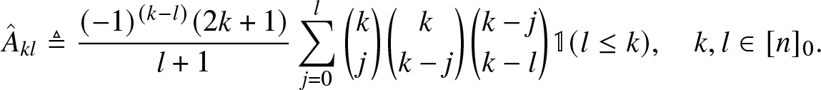
\hat{A}_{k l} \triangleq \frac{(-1)^{(k-l)}(2k+1)}{l+1} \sum_{j = 0}^{l} \binom{k}{j} \binom{k}{k-j} \binom{k-j}{k-l}\mathbb{1}(l\leq k), \quad k, l \in [n]_0.
\end{align}
\begin{align}
\hat{A}_{k l} \triangleq \frac{(-1)^{(k-l)}(2k+1)}{l+1} \sum_{j = 0}^{l} \binom{k}{j} \binom{k}{k-j} \binom{k-j}{k-l}\mathbb{1}(l\leq k), \quad k, l \in [n]_0.
\end{align}  $\hat{\mathbf{A}}$ is a lower triangular matrix. As for the BM method, the transform matrix needs to be calculated only once for the desired level of accuracy, and the above matrix-vector multiplication requires $\frac{(n+1)(n+2)}{2}$ multiplications. Further details about the accuracy requirements are provided in Section 4.6.
4. Generation of moment sequences and performance evaluation
To compare the performance of different HMTs, moment sequences and corresponding functions serving as the ground truth are needed. Generating representative moment sequences is non-trivial since the probability that a sequence uniformly distributed on  $[0,1]^n$ is a moment sequence is about $2^{-n^2}$ [Reference Chang, Kemperman and Studden1, Eq. 1.2]. In this section, we provide three different ways to solve it: The first method generates uniformly distributed integer moment sequences, while the other two generate moments from either analytic expressions of moments or analytic expressions of cdfs. In these two cases, the parameters are randomized. We use the exact cdf as the reference function if it is given by analytic expressions. Otherwise, we use the GP approximations as the reference functions.
4.1. Moment sequences and their rates of decay
As discussed in Section 3.1, the CM method can fully recover discrete distributions with a finite number of jumps, while other methods, such as the ME method, cannot. This indicates that different HMTs may have different performance for different types of distributions, classified by the decay order of the sequence. We first provide some examples of moment sequences from common distributions.
Example 4.1. (Beta distributions) For  $X \sim \operatorname{Beta}(\alpha, \beta)$,
 \begin{align}
m_n & =\prod_{r = 0}^{n-1} \frac{\alpha +r}{\alpha + \beta +r} = \frac{\Gamma(\alpha + n ) }{\Gamma(\alpha ) } \frac{\Gamma(\alpha + \beta ) }{\Gamma(\alpha + \beta +n ) }.
\end{align}
\begin{align}
m_n & =\prod_{r = 0}^{n-1} \frac{\alpha +r}{\alpha + \beta +r} = \frac{\Gamma(\alpha + n ) }{\Gamma(\alpha ) } \frac{\Gamma(\alpha + \beta ) }{\Gamma(\alpha + \beta +n ) }.
\end{align} By Stirling’s formula, as  $n \to \infty$,
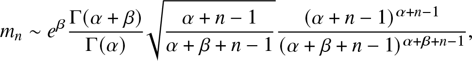 \begin{align}
m_n & \sim e^\beta\frac{\Gamma(\alpha + \beta ) }{\Gamma(\alpha ) }\sqrt{\frac{\alpha + n-1}{\alpha + \beta + n-1}} \frac{(\alpha + n-1)^{\alpha + n-1} }{ (\alpha + \beta + n-1)^{\alpha + \beta + n-1}},
\end{align}
\begin{align}
m_n & \sim e^\beta\frac{\Gamma(\alpha + \beta ) }{\Gamma(\alpha ) }\sqrt{\frac{\alpha + n-1}{\alpha + \beta + n-1}} \frac{(\alpha + n-1)^{\alpha + n-1} }{ (\alpha + \beta + n-1)^{\alpha + \beta + n-1}},
\end{align}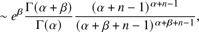 \begin{align}
& \sim e^\beta \frac{\Gamma(\alpha + \beta ) }{\Gamma(\alpha ) } \frac{(\alpha + n-1)^{\alpha + n-1}}{(\alpha + \beta + n-1)^{\alpha + \beta + n-1}},
\end{align}
\begin{align}
& \sim e^\beta \frac{\Gamma(\alpha + \beta ) }{\Gamma(\alpha ) } \frac{(\alpha + n-1)^{\alpha + n-1}}{(\alpha + \beta + n-1)^{\alpha + \beta + n-1}},
\end{align}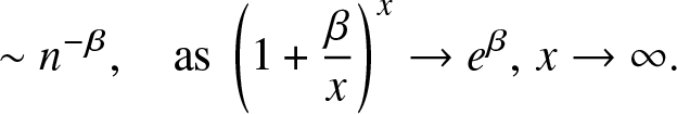 \begin{align}
& \sim n^{-\beta}, \quad \text{as } \left(1+\frac{\beta}{x}\right)^{x} \to e^\beta, \, x\to \infty.
\end{align}
\begin{align}
& \sim n^{-\beta}, \quad \text{as } \left(1+\frac{\beta}{x}\right)^{x} \to e^\beta, \, x\to \infty.
\end{align} Thus,  $m_n = \Theta(n^{-\beta})$.
Example 4.2. Let the density function be  $f(x) = 2 x/s^2 \mathbf{1}_{[0,s]}(x)$ with $0 \lt s \lt 1$. Then $m_n = 2 s^n /(n+2) = O(\exp(-\log(1/s) n )) = \Omega(\exp(-s_1 n ))$ for all $s_1 \gt \log(1/s)$.
Given the examples shown above and that the performance of different HMTs is likely to be dependent on the rate of decay (or type of decay) of the moment sequences, we would like to develop a method to categorize different moment sequences based on their tail behavior. To this end, we introduce six types of moment sequences based on their rates of decay.
Definition 4.3. (Rate of decay)
1. Sub-power-law decay: In this case, for all s > 0,
$m_n = \Omega(n^{-s})$.2. Power-law decay: In this case, there exists s > 0 such that
$m_n = \Theta(n^{-s})$.3. Soft power-law decay: In this case,
$m_n \neq \Theta(n^{-s}), \,\forall s \geq 0$ but there exist
$s_1 \gt s_2 \geq 0$ such that
$m_n = \Omega(n^{-s_1})$ and
$m_n = O(n^{-s_2})$.4. Intermediate decay: In this case, for all
$s_1 \geq 0$,
$m_n = O(n^{-s_1})$ and for all
$s_2 \gt 0$,
$m_n = \Omega(\exp(-s_2 n))$.5. Soft exponential decay: In this case,
$m_n \neq \Theta(\exp(-s n)), \, \forall s \gt 0$ but there exists
$s_1 \gt s_2 \gt 0$,
$m_n = \Omega(\exp(-s_1 n))$ and
$m_n = O(\exp(-s_2 n))$.6. Exponential decay: In this case, there exists s > 0 such that
$m_n = \Theta(\exp(-s n))$.


4.2. Uniformly random (integer) moment sequences
4.2.1. Generation
Let Λ denote the set of probability measures on  $[0,1]$. For $\lambda \in \Lambda$ we denote by
 \begin{align}
m_n(\lambda) \triangleq \int_{0}^{1} x^n \, d\lambda, \quad n \in \mathbb{N}_0,
\end{align}
\begin{align}
m_n(\lambda) \triangleq \int_{0}^{1} x^n \, d\lambda, \quad n \in \mathbb{N}_0,
\end{align} its n-th moment. Trivially,  $m_0(\lambda) = 1$, $\forall \lambda \in \Lambda$. The set of all moment sequences is defined as
 \begin{align}
\mathcal{M} \triangleq \{\left(m_1(\lambda), m_2(\lambda), ...\right), \lambda \in \Lambda\}.
\end{align}
\begin{align}
\mathcal{M} \triangleq \{\left(m_1(\lambda), m_2(\lambda), ...\right), \lambda \in \Lambda\}.
\end{align} The set of the projection onto the first n coordinates of all elements in  $\mathcal{M}$ is denoted by $\mathcal{M}_n$.
Now we recall how to establish a one-to-one mapping from the moment space  $\operatorname{int} \mathcal{M}$ onto the set $(0,1)^\mathbb{N}$ [Reference Chang, Kemperman and Studden1], where $\operatorname{int} \mathcal{M}$ denotes the interior of the set $\mathcal{M}$. For a given sequence $\left(m_k\right)_{k \in [n-1]} \in \mathcal{M}_{n-1}$, the achievable lower and upper bounds for mn are defined as
 \begin{align}
m_n^- \triangleq \min \{m_n(\lambda), \lambda \in \Lambda \text{with } m_k(\lambda) = m_k \text{for } k \in [n-1]\},
\end{align}
\begin{align}
m_n^- \triangleq \min \{m_n(\lambda), \lambda \in \Lambda \text{with } m_k(\lambda) = m_k \text{for } k \in [n-1]\},
\end{align} \begin{align}
m_n^+ \triangleq \max \{m_n(\lambda), \lambda \in \Lambda \text{with } m_k(\lambda) = m_k \text{for } k \in [n-1]\}.
\end{align}
\begin{align}
m_n^+ \triangleq \max \{m_n(\lambda), \lambda \in \Lambda \text{with } m_k(\lambda) = m_k \text{for } k \in [n-1]\}.
\end{align} Note that  $m_1^- =0 $ and $m_1^+ = 1$. $m_n^-$ and $m_n^+$, $n \geq 2$, can be obtained by taking the infimum and supremum of the range obtained from solving the two linear inequalities $0\leq \underline{H}_{n}$ and $ 0\leq \overline{H}_{n}$.
We now consider the case where  $\left(m_k\right)_{k \in [n-1]} \in \operatorname{int} \mathcal{M}_{n-1}$, that is, $m_n^+ \gt m_n^-$. The canonical moments are defined as
 \begin{align}
p_n \triangleq \frac{m_n - m_n^-}{m_n^+ - m_n^-}.
\end{align}
\begin{align}
p_n \triangleq \frac{m_n - m_n^-}{m_n^+ - m_n^-}.
\end{align}  $\left(m_k\right)_{k \in [n]} \in \operatorname{int} \mathcal{M}_n$ if and only if $p_n \in (0,1)$ [Reference Chang, Kemperman and Studden1, Reference Dette and Studden2]. In this way, pn represents the relative position of mn among all the possible n-th moments given the sequence $\left(m_k\right)_{k \in [n-1]} $. The following theorem from [Reference Chang, Kemperman and Studden1] shows the relationship between the distribution on the moment space $\mathcal{M}_n$ and the distribution of pk, $k \in [n]$.
Theorem 4.4 ([Reference Chang, Kemperman and Studden1, Thm. 1.3]) For a uniformly distributed random vector  $\left(m_k\right)_{k \in [n]} $ on the moment space $\mathcal{M}_n$, the corresponding canonical moments pk, $k \in [n]$, are independent and beta distributed as
 \begin{align*}
p_k \sim \mathrm{Beta}(n - k +1, n-k+1), \quad k \in [n].
\end{align*}
\begin{align*}
p_k \sim \mathrm{Beta}(n - k +1, n-k+1), \quad k \in [n].
\end{align*} Since  $\mathcal{M}_n$ is a closed convex set, its boundary has Lebesgue measure zero. Therefore, although (4.9) only defines the mapping on $\operatorname{int} \mathcal{M}_n$, the pk are still well defined.
Theorem 4.4 provides a method to generate uniformly random moment sequences. The details are summarized in the following algorithm.
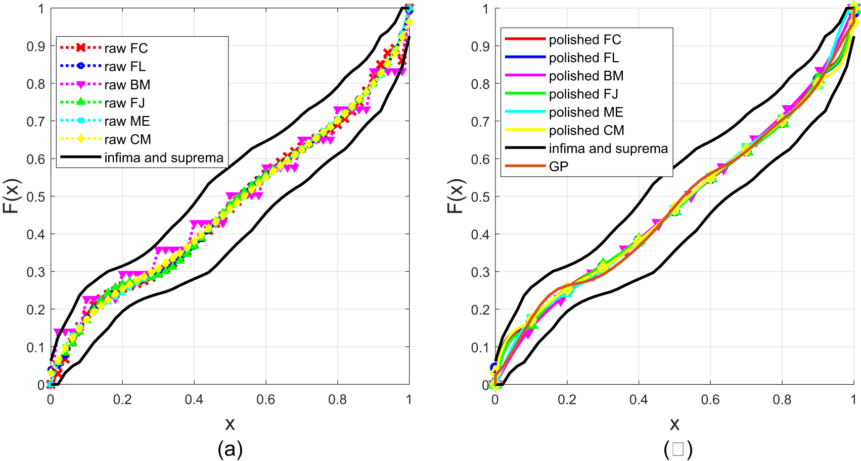
Figure 11. An example of the reconstructed cdf of each method. The 10 moments are randomly generated by the canonical moments and the moments are 0.5256, 0.3893, 0.3188, 0.2747, 0.2442, 0.2215, 0.2038, 0.1895, 0.1775, and 0.1674. The polished curves are obtained after the tweaking mapping in Definition 2.2 as well as the monotone cubic interpolation for  $\hat{F}_{\rm{BM},10}|_{\mathcal{U}_{11}}$, $\hat{F}_{\rm{ME},10}|_{\mathcal{U}_{10}}$, $\hat{F}_{\rm{FJ},10}|_{\mathcal{U}_{10}}$, $\hat{F}_{\rm{FL},{9}}|_{\mathcal{U}_{10}}$, $\hat{F}_{\rm{FC},9}|_{\mathcal{U}_{10}}$, and $\hat{F}_{\rm{CM},10}|_{\mathcal{U}_{10}}$ (a) Raw curves. (b) Polished curves.
4.2.2. Usage
Figure 11(a) shows an example of the reconstructed cdfs (only raw versions) of each method, where moments generated by Algorithms 1 and 10 are used. But since a reference function serving as the ground truth is missing, we cannot compare the performance of each method. It is natural to look for a way to reconstruct a solution to the HMT via (infinitely many) integer moments. However, no known reconstruction methods exist for integer moments. To address this problem, we take a detour to approximate the characteristic function first, and then apply the GP theorem to reconstruct the cdf [Reference Gil-Pelaez3]. Let  $X \in [0,1]$ denote the random variable and $(m_n)_{n=0}^{\infty}$ denote its moments. The characteristic function of X is
 \begin{align}
\phi_X(s) & = \mathbb{E}[\exp(jsX)], \quad s\in \mathbb{R}^+.
\end{align}
\begin{align}
\phi_X(s) & = \mathbb{E}[\exp(jsX)], \quad s\in \mathbb{R}^+.
\end{align}Written in terms of its Taylor expansion,
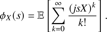 \begin{align}
\phi_X(s) & = \mathbb{E}\left[\sum_{k = 0}^{\infty} \frac{(jsX)^k}{k!}\right].
\end{align}
\begin{align}
\phi_X(s) & = \mathbb{E}\left[\sum_{k = 0}^{\infty} \frac{(jsX)^k}{k!}\right].
\end{align} By the dominated convergence theorem, we can change the order of expectation and summation, that is, for any  $s \in [0,\infty)$
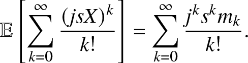 \begin{align}
\mathbb{E}\left[\sum_{k = 0}^{\infty} \frac{(jsX)^k}{k!}\right] & = \sum_{k = 0}^{\infty} \frac{j^k s^k m_k}{k!}.
\end{align}
\begin{align}
\mathbb{E}\left[\sum_{k = 0}^{\infty} \frac{(jsX)^k}{k!}\right] & = \sum_{k = 0}^{\infty} \frac{j^k s^k m_k}{k!}.
\end{align} The imaginary moments of X, mjs, are the characteristic function of  $\log(X)$. When applied to $X \sim \exp(1)$, the expansion in (4.12) yields the gamma function, which is consistent with the analytic continuation property of the moments.
The truncated sum
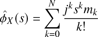 \begin{align}
\hat{\phi}_X(s) = \sum_{k = 0}^{N} \frac{j^k s^k m_k}{k!}
\end{align}
\begin{align}
\hat{\phi}_X(s) = \sum_{k = 0}^{N} \frac{j^k s^k m_k}{k!}
\end{align} approximates the characteristic function  $\phi_X(s)$, and, in turn, the integral
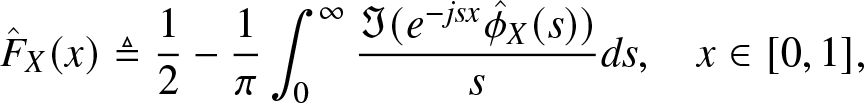 \begin{align}
\hat{F}_X(x) & \triangleq \frac{1}{2} - \frac{1}{\pi} \int_0^\infty \frac{\Im{(e^{-jsx}\hat{\phi}_X(s))}}{s} ds, \quad x \in [0,1],
\end{align}
\begin{align}
\hat{F}_X(x) & \triangleq \frac{1}{2} - \frac{1}{\pi} \int_0^\infty \frac{\Im{(e^{-jsx}\hat{\phi}_X(s))}}{s} ds, \quad x \in [0,1],
\end{align}is an approximation of the exact cdf
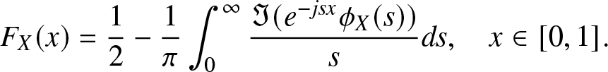 \begin{align}
{F}_X(x) & = \frac{1}{2} - \frac{1}{\pi} \int_0^\infty \frac{\Im{(e^{-jsx}{\phi}_X(s))}}{s} ds, \quad x \in [0,1].
\end{align}
\begin{align}
{F}_X(x) & = \frac{1}{2} - \frac{1}{\pi} \int_0^\infty \frac{\Im{(e^{-jsx}{\phi}_X(s))}}{s} ds, \quad x \in [0,1].
\end{align} Therefore, by evaluating (approximating)  $\hat{F}_X$, we obtain an approximation of the exact cdf ${F}_X$.
Figure 11(b) shows the reconstructions by the above method and all the HMTs. We observe that all the HMTs approximate well. However, even though the series converges for  $s \in [0,\infty)$, the evaluation of each element with alternating signs could cause serious numerical problems, as s increases. For each s, we need at least $N = \lceil{se}\rceil$ to approximate $\phi_X(s)$ so that the absolute error is within $\sqrt{2/(\pi N)}$. Meanwhile, an accurate evaluation of $\hat{F}_X$ usually requires the calculation of the integrand up to $s = 1,000$. This requires the calculation of $N = 2,719$ moments, which is time-consuming and not practical for the performance evaluation purposes in Section 4.5.
4.3. Generating moments by analytic expressions
As we need to generate moment sequences of variable lengths, it is natural to directly start with the infinite sequences  $(m_n)_{n=0}^{\infty}$ and truncate them to the desired length.
We first recall the definition of completely monotonic functions.
Definition 4.5. (Completely monotonic function [Reference Widder30]) A function f is said to be c.m. on an interval I if f is continuous on I and has derivatives of all orders on  $\operatorname{int} I$ (the interior of I) and for all $n \in \mathbb{N}$,
 \begin{align}
(-1)^n f^{(n)}(x) \geq 0, \quad x\in \operatorname{int} I.
\end{align}
\begin{align}
(-1)^n f^{(n)}(x) \geq 0, \quad x\in \operatorname{int} I.
\end{align} The sequence  $(f(k))_{k=0}^\infty$ is c.m. if f is c.m. on $[0,\infty)$ [Reference Widder30]. Thus, we can use c.m. functions to generate moment sequences.
Based on the six types of moment sequences discussed in Section 4.1, we define six classes of c.m. functions that decay at different rates.
Definition 4.6. (Six classes of c.m. functions) Based on the definition of rate of decay in Definition 4.3, we define the following c.m. functions.
• Sub-power-law decay
$\Omega(n^{-s})$:
$F_1(n; a, s) \triangleq a^s (\log(n + 1) + a)^{-s}$.• Power-law decay
$\Theta(n^{-s})$:
$F_2(n;a,s) \triangleq a^s (n+a)^{-s} $.• Soft power-law decay:
$F_3 (n; a, b, s) \triangleq a^s b (n+a)^{-s} (\log(n+1) + b)^{-1}$.• Intermediate decay:
$F_4(n; a, s) \triangleq \exp( s \sqrt{a} - s \sqrt{n+a})$.• Soft exponential decay:
$F_5(n; a, s) \triangleq \exp(-sn)a (n+a)^{-1} $.• Exponential decay
$\Theta(\exp(-s n ))$:
$F_6(n; s) \triangleq \exp( -sn)$.


 $s \in \mathbb{R}^+$ is referred to as the rate, and $a\in \mathbb{R}^+$ and $b \in \mathbb{R}^+$ (if present) are referred to as the other parameters.
For moment sequences  $(m_{i,n})_{n = 0}^{\infty}$, $i = 1,..., N$, the convex combination $m_n = \sum_{i = 1}^N c_i m_{i,n}$, where $\sum_{i = 1}^N c_i = 1$, $c_i \gt 0$, remains c.m. Hence, $(m_n)_{n = 0}^{\infty}$ is also a moment sequence.
Now, we introduce our algorithm to generate  $(m_n)_{n = 0}^k$ with a desired rate of decay s and flexibility in the other parameters, that is, a and/or b. Since the c.m. functions are analytic, the c.m. function of integer moments can be easily extended to complex moments by analytic continuation. To obtain complex moments mz, we just need to replace n in steps 2 and 3 of Algorithm 2 with $z \in \mathbb{C}$.
Algorithm 2. Algorithm for moment sequences by c.m. functions
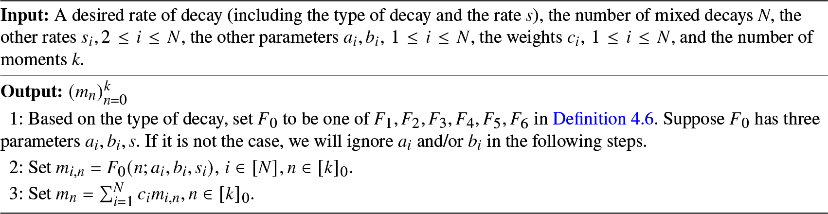
To deterministically generate moments by Algorithm 2, we need to fix  $s \gt 0, N \in \mathbb{N}, s_i \gt s, 2\leq i \leq N$ for the exponential decay and $s_i = s$ for the others, $a_i, b_i, c_i \gt 0$ and $\sum_{i = 1}^N c_i = 1$.
To randomly generate moments by Algorithm 2, we first choose  $s\sim \mathrm{Uniform}(0,10)$ except for the exponential and soft exponential cases, where $s\sim -\log\left(\mathrm{Uniform}(0,1)\right)$. We set $s_i = s$ except that $ s_1 = s, s_i \sim -\log\left( \mathrm{Uniform} (0,\exp(-s))\right), 2\leq i \leq N$ for the exponential decay. Next, we randomly generate N from the set $\{1,2,..., 10\}$. Then we choose $a_i, b_i \sim \mathrm{Uniform} (0,10), \,1\leq i \leq N$. Finally, we choose $c_i \sim \mathrm{Uniform}(0,10)$ and normalize them so that the sum is 1. In this way, we have at least 2N degrees of freedom.
Similar to Section 4.2.1, the exact cdf is unknown. We use the GP approximations as a reference when making comparisons.
4.4. Generating moments by known distributions
Beta distributions are continuous probability distributions supported on  $[0,1]$. Here, we use the beta mixture model to randomly generate distributions. The pdf of N beta mixtures is
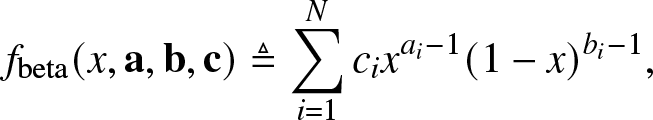 \begin{align}
f_{\rm{beta}}(x,\mathbf{a, b, c}) \triangleq \sum_{i = 1}^N c_i x^{a_i - 1}(1-x)^{b_i - 1},
\end{align}
\begin{align}
f_{\rm{beta}}(x,\mathbf{a, b, c}) \triangleq \sum_{i = 1}^N c_i x^{a_i - 1}(1-x)^{b_i - 1},
\end{align} where  $\mathbf{a} \triangleq (a_i)_{i = 1}^N, \mathbf{b} \triangleq (b_i)_{i = 1}^N, \mathbf{c} \triangleq (c_i)_{i = 1}^N$, $\mathbf{a, b, c} \succ \mathbf{0}$ and $\sum_{i = 1}^N c_i = 1$. The n-th moment is
 \begin{align}
m_n = \sum_{i = 1}^N c_i\prod_{r=0}^{n-1} \frac{a_i+r}{a_i+b_i+r},
\end{align}
\begin{align}
m_n = \sum_{i = 1}^N c_i\prod_{r=0}^{n-1} \frac{a_i+r}{a_i+b_i+r},
\end{align}and the cdf is
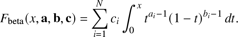 \begin{align}
F_{\rm{beta}}(x,\mathbf{a, b, c}) = \sum_{i = 1}^N c_i \int_{0}^{x}t^{a_i - 1}(1-t)^{b_i - 1}\, dt.
\end{align}
\begin{align}
F_{\rm{beta}}(x,\mathbf{a, b, c}) = \sum_{i = 1}^N c_i \int_{0}^{x}t^{a_i - 1}(1-t)^{b_i - 1}\, dt.
\end{align} By randomly choosing  $\mathbf{a, b, c} $, we are able to randomly generate the distribution and thus randomly generate the imaginary and integer moment sequences by definition. We first randomly generate N from the set $\{1,2,..., 10\}$.Footnote 6 Then we choose $a_i, b_i \sim \mathrm{Uniform} (0,10), \,1\leq i \leq N$. Finally, we choose $c_i \sim \mathrm{Uniform}(0,10)$ and normalize them so that the sum is 1.
4.5. Performance evaluation
Using the moments randomly generated in Section 4.3, we compare the performance of the different Hausdorff moment transforms. Since the actual cdfs are not available in this case, we use the cdfs obtained by the GP method as the reference.Footnote 7
For all methods except the GP, BM, FL, and FC methods, we consider  $F_{\rm{method},n}|_{\mathcal{U}_n}$. For the GP method, we consider $F_{\rm{GP}}|_{\mathcal{U}_{150}}$, for the BM method, we consider $F_{\rm{BM},n}|_{\mathcal{U}_{n+1}}$, and for the FL and FC methods, we consider $F_{\rm{method},n-1}|_{\mathcal{U}_{n}}$. We apply the tweaking mapping in Definition 2.2 followed by monotone cubic interpolation.
In Figure 12, we plot the average of the total distance versus the number of moments (m 0 is not counted) for different methods and different types of decays. For practical purposes regarding accuracy requirements in moments and basic operations and the difficulty in finding roots of polynomials, the number of moments of the FJ, FL, FC, and ME methods is limited to 50, the number of moments of the CM method is limited to 30, and the number of moments of the BM method is limited to 150. We observe that the average of the total distance of all the methods except the FJ and the ME methods decreases as the number of moments increases. In most cases, the average of the total distance of the FJ method does not decrease since it is not guaranteed to converge. As for the ME method, although it converges in entropy, it suffers from the problem of finding the minimum in (3.4). Even if some of the curves in Figure 12 show a decreasing trend, we cannot rely on this method as long as we cannot make sure the results we get from solving (3.4) are the minima, that is, the size of the gradient is less than the value of the optimality tolerance. In terms of their best possible performance, we also observe that the CM method is great for all types of decays, especially the exponential and soft exponential decays. For the exponential decay, the moments are from discrete distributions that have no more than 10 jumps. Thus, the raw CM method of order 20 is able to fully characterize the distributions by identifying jump locations and jump heights. Our comparisons are made based on the decay type. However, in practice, it is impossible to determine the decay type given the values of the moments. Thus, for practical purposes, it is preferable to utilize methods that work well overall. Among all the methods, the FL and FC methods have overall good performance and the FL method even outperforms the CM method in the power-law decay.

Figure 12. The average of the total distance versus the number of moments for different methods and different types of decays. Averaging is performed over 100 randomly generated moment sequences (a) Sub power-law decay (b) Power-law decay (c) Soft power-law decay (d) Intermediate decay (e) Exponential decay (f) Soft exponential decay.
Figure 13 shows computation time versus the number of moments for the power-law decay and it is similar for the other types. In Figure 13(a), the computation time of the FL, FC, and BM method is based on the original implementation, whereas in Figure 13(b), it is based on the linear transform with the pre-calculated transform matrices. In Figure 13(b), for all methods except the CM method, the computation time increases quadratically with the number of moments. This is consistent with the order of matrix-vector multiplication for the FL, FC, and BM method. Furthermore, with the linear transform, the computation time for the FL, FC, and BM method in Figure 13(a) is significantly reduced compared to that in Figure 13(a). Even for small values of n, such as 10, 20, and 30, the CM method’s computation time is at least ten times longer than that of the other methods for the same number of moments. As n increases, the computation time of the CM method is expected to grow even more, making it unsuitable for time-sensitive applications.
As shown in Example 4.1, the moment sequences generated by Section 4.4 exhibit power-law decay. Its results are similar to those in Figure 12(a).
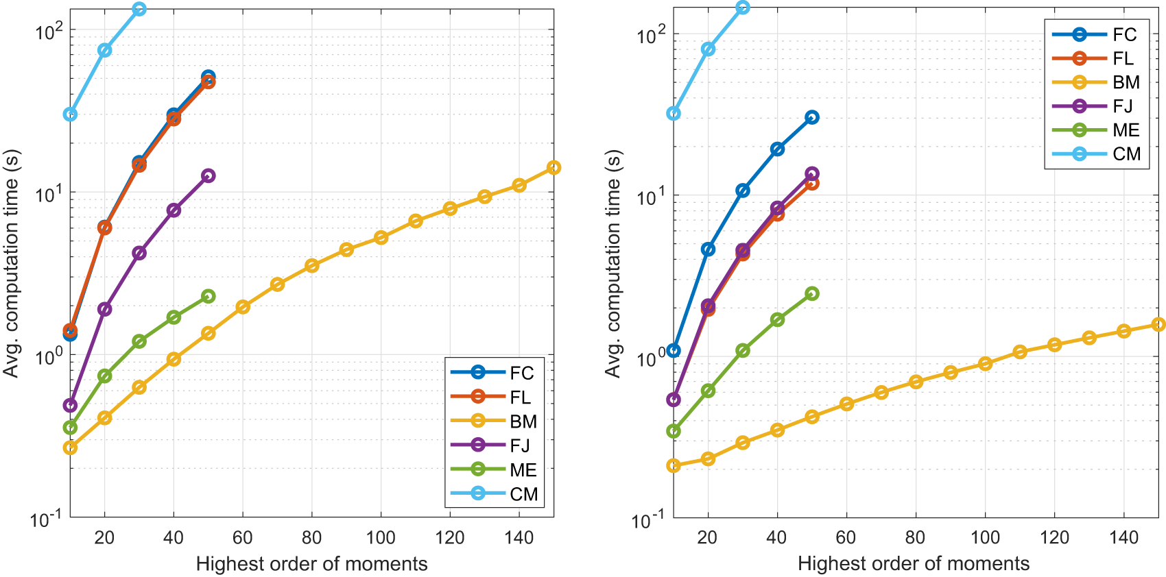
Figure 13. The average computation time versus the number of moments. Averaging is performed over 100 randomly generated moment sequences of power-law decay: (a) original implementation and (b) linear transform.
4.6. Accuracy requirements for HMTs
The accuracy requirements apply to both of the coefficients of the moments and the HMTs, such as the transform matrices for the BM and FL method. Here we just mention some typical requirements.
Accuracy requirements for transform matrices: For the BM method of order n, as  $\max \|\mathbf{A}\| \sim \frac{\sqrt{27}}{2\pi} \frac{3^n}{n}$, $n \to \infty$, about $n/2 - \log_{10} n$ decimal digits are needed [Reference Haenggi6]. For the FL method of order n, as $\max \|\hat{\mathbf{A}}\| \leq \binom{2n}{n}\binom{n}{n/3} \sim \frac{3^{n+1}2^{4n/3}}{4\pi n}$, $n \to \infty$, about 0.9n decimal digits are sufficient.
Accuracy requirements for moments in Definition 4.6: For the power-law decay, about  $s \log_{10} \frac{n+a}{a}$ decimal digits are needed. For exponential decay, about $sn/2$ decimal digits are needed.
The calculation can be carried out in the logarithm domain which may reduce the accuracy requirement. Moreover, the matrix multiplication of the FL method is pre-calculated, that is,  $\hat{\mathbf{A}} \mathbf{1}$, and $\hat{\mathbf{A}} \hat{\mathbf{m}}$ are done separately.
5. Conclusion
The truncated Hausdorff moment problem is both fundamental and practically relevant. While several theoretical methods for its solutions have been proposed, a systematic study and comparison of their performance and details in their numerical implementation has been missing. This work provides these important missing pieces by discussing advantages and drawbacks of different methods, comparing convergence properties, and proposing a tweaking method to ensure the resulting functions satisfy the properties of probability distributions. In addition, two new methods are introduced that compare favorably with known ones. For a fair comparison, three methods for the random generation of moment sequences are discussed or proposed, so that the distances between approximated and actual distributions can be averaged over many realizations of moment sequences. It turns out that the decrease of the distances as a function of the number of moments depends strongly on the type of decay of the moment sequences. For this reason, we introduced a classification of the decay order in six classes. Our work also reveals the trade-off between performance and computational cost. If high accuracy is desired (at higher computational effort), the FC and FL methods are good choices, with the FC method having the advantage of uniform convergence; if computational resources are limited, the BM method is preferred.
Funding statement
This work was supported in part by the US National Science Foundation through Grant 2007498.
Competing interest
None.


 Open access