


1 Introduction
Item factor analysis (IFA; e.g., Bock et al., Reference Bock, Gibbons and Muraki1988; Wirth & Edwards, Reference Wirth and Edwards2007) is a powerful statistical framework used to model and measure latent variables. The latent variables can be mathematical ability (Rutkowski et al., Reference Rutkowski, von Davier and Rutkowski2013), mental disorder (Stochl et al., Reference Stochl, Jones and Croudace2012), or personality traits (Balsis et al., Reference Balsis, Ruchensky and Busch2017) that influence individuals’ responses to various items, such as test or survey questions. IFA aims to uncover these hidden factors by analyzing patterns in the responses, allowing researchers to understand the relationships between the latent variables and the items. Understanding these latent structures is crucial across fields, such as psychology and education for accurate measurement of human abilities and characteristics (Chen et al., Reference Chen, Li, Liu and Ying2021; Wirth & Edwards, Reference Wirth and Edwards2007).
Psychological and educational research now frequently involves diverse data types, including large-scale assessment, high-volume data, and process data involving unstructured and textual responses (e.g., Ma et al., Reference Ma, Ouyang, Wang and Xu2024; Weston & Laursen, Reference Weston and Laursen2015; Zhang et al., Reference Zhang, Wang, Qi, Liu and Ying2023). Traditional estimation algorithms often struggle to efficiently process and analyze these data, leading to unstable model estimates, long computation times, and excessive memory usage. Deep learning (DL) literature has much to offer to handle the above challenges. If we view IFA from the lens of generalized latent variable models (Muthén, Reference Muthén2002; Rabe-Hesketh & Skrondal, Reference Rabe-Hesketh and Skrondal2008), representation learning (Bengio et al., Reference Bengio, Courville and Vincent2013) can help model and capture intricate latent patterns from observed data. Unlike traditional IFA estimation methods, which often rely on strict parametric and distributional assumptions, representation learning leverages powerful learning algorithms and expressive models such as neural networks to generate richer and highly flexible representations when modeling data. This improves the modeling and detection of subtle patterns for high-dimensional latent variables that classical methods might underfit. Therefore, by integrating representation learning with IFA, researchers can achieve a more comprehensive understanding of latent traits.
One of the representation techniques that is being actively applied in IFA (Cho et al., Reference Cho, Wang, Zhang and Xu2021; Hui et al., Reference Hui, Warton, Ormerod, Haapaniemi and Taskinen2017; Jeon et al., Reference Jeon, Rijmen and Rabe-Hesketh2017) is variants based on variational autoencoders (VAEs; Curi et al., Reference Curi, Converse, Hajewski and Oliveira2019; Wu et al., Reference Wu, Davis, Domingue, Piech and Goodman2020). VAEs consist of two main components: an encoder and a decoder. The encoder network compresses the high-dimensional input data into a lower-dimensional latent space, effectively capturing the essential features that define the data’s underlying structure. Conversely, the decoder network reconstructs the original data from these latent representations, ensuring that the compressed information retains the critical characteristics. Urban & Bauer (Reference Urban and Bauer2021) further incorporated an importance-weighted (IW) approach (Burda et al., Reference Burda, Grosse and Salakhutdinov2015) to improve the estimation performance of VAEs in IFA. These advances have an advantage over the traditional techniques, such as Gauss–Hermite quadrature or the EM algorithm (Bock & Aitkin, Reference Bock and Aitkin1981; Cai, Reference Cai2010; Darrell Bock & Lieberman, Reference Darrell Bock and Lieberman1970) for large sample size and models with high-dimensional latent variables.
Despite the significant advancements brought by VAEs in IFA, conventional VAEs may inadequately capture the true posterior distribution due to insufficiently expressive inference models (Mescheder et al., Reference Mescheder, Nowozin and Geiger2017). Specifically, VAEs might focus on the modes of the prior distribution and fail to represent the latent variables in some local regions (Makhzani et al., Reference Makhzani, Shlens, Jaitly, Goodfellow and Frey2015). Consequently, enhancing the expressiveness of the approximate posterior is imperative for improved performance (Cremer et al., Reference Cremer, Li and Duvenaud2018).
An alternative representation paradigm, generative adversarial networks (GANs; Goodfellow et al., Reference Goodfellow, Pouget-Abadie, Mirza, Xu, Warde-Farley, Ozair, Courville and Bengio2014), a celebrated framework for estimating generative models in DL and computer vision, offer greater flexibility in modeling arbitrary probability densities and can contribute to the expressiveness. Multiple variants of GANs have achieved remarkable success in complex tasks, such as image generation (e.g., Arjovsky et al., Reference Arjovsky, Chintala and Bottou2017; Radford, Reference Radford2015; Zhu, Park, et al., Reference Zhu, Park, Isola and Efros2017). Among these models, the combination of GANs and VAEs can be traced back to adversarial autoencoders (AAEs; Makhzani et al., Reference Makhzani, Shlens, Jaitly, Goodfellow and Frey2015) and the VAE-GAN model (Larsen et al., Reference Larsen, Sønderby, Larochelle and Winther2016). Figure 1 provides an intuitive visual example demonstrating how integrating GANs and VAEs can lead to better representation learning. The figure compares ten handwritten images sampled from four models: (a) GAN, (b) WGAN (a GAN variant, Arjovsky et al., Reference Arjovsky, Chintala and Bottou2017), (c) VAE, and (d) VAE-GAN. While GAN generated only the digit 1,Footnote 1 WGAN exhibited unstable performance, and the images produced by VAE appeared blurry. In contrast, VAE-GAN generated relatively clear results for most of digits. However, vanilla GANs, VAE-GANs, and AAEs rely solely on adversarial loss, formulated as a minimax game between networks to deceive a discriminator. As a result, they are not motivated from a maximum-likelihood perspective and are therefore not directly applicable for improving marginal maximum likelihood (MML) estimation in IFA.

Figure 1 Ten handwritten images sampled from model (a) GAN, (b) WGAN, (c) VAE, and (d) VAE-GAN. Adapted from Mi et al. (Reference Mi, Shen and Zhang2018).
Therefore, this article focuses on an improved approach based on VAEs, adversarial variational Bayes (AVB; Mescheder et al., Reference Mescheder, Nowozin and Geiger2017), which has a flexible and general approach to construct inference models. AVB improves the traditional VAE framework by integrating elements from GANs, specifically by introducing an auxiliary discriminator network. This discriminator engages in an adversarial training process with the encoder to help the inference model produce more accurate and expressive latent variable estimates. By combining the strengths of both VAEs and GANs, AVB removes the restrictive assumption of standard normal distributions in the inference model and enables effective exploration of complex, multimodal latent spaces. Theoretical and empirical evidence has shown that AVB can achieve higher log-likelihood, lower reconstruction error, and more precise approximation of the posterior (Mescheder et al., Reference Mescheder, Nowozin and Geiger2017). For example, we consider a simple dataset containing samples from four different labels whose latent codes are uniformly distributed. Figure 2 compares the recovered latent distribution: the unallocated regions (“empty space”) and overlap between regions in VAE’s result can yield ambiguous latent codes and compromise both inference precision and the quality of generated samples, but AVB produces a posterior with well-defined boundaries around each region. This approach not only improves the flexibility and accuracy of MML estimation but also provides more potential for better handling more diverse and high-dimensional data that become increasingly common in psychological and educational research.

Figure 2 Distribution of latent variables for VAE and AVB trained on a simple synthetic dataset containing samples from four different labels.
This study proposes an innovative algorithm combining IWAE (IWAE; Burda et al., Reference Burda, Grosse and Salakhutdinov2015) with AVB to enhance the estimation of parameters for more general and complex IFA. The proposed algorithm can be regarded as an improvement of the IWAE algorithm by Urban & Bauer (Reference Urban and Bauer2021). The main contributions are two-fold: (1) the novel importance-weighted AVB (IWAVB) method is proposed for exploratory and confirmatory IFA of polytomous item response data and (2) compared with the IWAE method, which is the current state-of-the-art and was shown to be more efficient than the classical Metropolis–Hastings Robbins–Monro (MH-RM; Cai, Reference Cai2010), numerical experiment results support similarly satisfactory performance of IWAVB, with improvement when the latent variables have a multimodal distribution.
The remaining parts are organized as follows. Section 2 explains how AVB builds upon traditional VAE methods for parameter estimation for the graded response model (GRM), a general framework within IFA. Section 3 details the implementation steps of the AVB algorithm and introduces strategies for improving its overall performance. Section 4 then provides a comparative evaluation of AVB and VAE, using both empirical and simulated data. Finally, Section 5 examines potential limitations of the proposed approach and highlights directions for future development.
2 Adversarial variational Bayes for item factor analysis
In the context of IFA, given the observed responses $\boldsymbol {x}$
, the variational inference (VI) method uses an inference model
$\boldsymbol {x}$
, the variational inference (VI) method uses an inference model $q_{\boldsymbol {\phi }}(\boldsymbol {z}\mid \boldsymbol {x})$
to approximate the posterior distribution of the latent variable
$q_{\boldsymbol {\phi }}(\boldsymbol {z}\mid \boldsymbol {x})$
to approximate the posterior distribution of the latent variable ${p_{\boldsymbol {\theta }}(\boldsymbol {z}\mid \boldsymbol {x})}$
. The
${p_{\boldsymbol {\theta }}(\boldsymbol {z}\mid \boldsymbol {x})}$
. The $\boldsymbol {\phi }$
represents the parameters for the inference model, and
$\boldsymbol {\phi }$
represents the parameters for the inference model, and ${\boldsymbol {\theta }}$
includes the parameters for the posterior distributions (e.g., items’ parameters). As a specific approach to perform VI, AVB can be regraded as an improved version of VAE which constructs more expressive inference model
${\boldsymbol {\theta }}$
includes the parameters for the posterior distributions (e.g., items’ parameters). As a specific approach to perform VI, AVB can be regraded as an improved version of VAE which constructs more expressive inference model $q_{\boldsymbol {\phi }}(\boldsymbol {z}\mid \boldsymbol {x})$
, and is shown to improve the likelihood estimation of parameters for the GRM in this section.
$q_{\boldsymbol {\phi }}(\boldsymbol {z}\mid \boldsymbol {x})$
, and is shown to improve the likelihood estimation of parameters for the GRM in this section.
2.1 The graded response model
The GRM (Samejima, Reference Samejima1969) is a specific model for IFA used for analyzing ordinal response data, particularly in psychological and educational measurement. The GRM assumes responses to an item are ordered categories (e.g., Likert scale). We follow the notation as in Cai (Reference Cai2010).
Given $i=1,\dots ,N$
distinct respondents and
$i=1,\dots ,N$
distinct respondents and $j=1,\dots ,M$
items, the response for respondent i to item j in
$j=1,\dots ,M$
items, the response for respondent i to item j in $C_j$
graded categories is
$C_j$
graded categories is $x_{i,j}\in \left \{0,1,\dots ,C_j-1\right \}$
. Assuming the number of latent variables is P, the
$x_{i,j}\in \left \{0,1,\dots ,C_j-1\right \}$
. Assuming the number of latent variables is P, the $P \times 1$
vector of latent variables for respondent i is denoted as
$P \times 1$
vector of latent variables for respondent i is denoted as $\boldsymbol {z}_i$
. For item j, the
$\boldsymbol {z}_i$
. For item j, the $P \times 1$
vector of loadings is
$P \times 1$
vector of loadings is $\boldsymbol {\beta }_j$
, and the
$\boldsymbol {\beta }_j$
, and the $(C_j-1)\times 1$
vector of strictly ordered category intercepts is
$(C_j-1)\times 1$
vector of strictly ordered category intercepts is $\boldsymbol {\alpha }_j=(\alpha _{j,1},\dots ,\alpha _{j,C_j-1})^T$
. Also, the parameters of item j are denoted as
$\boldsymbol {\alpha }_j=(\alpha _{j,1},\dots ,\alpha _{j,C_j-1})^T$
. Also, the parameters of item j are denoted as $\boldsymbol {\theta }_j=(\boldsymbol {\alpha }_j,\boldsymbol {\beta }_j)$
. The GRM is defined as the boundary probability conditional on the item parameters
$\boldsymbol {\theta }_j=(\boldsymbol {\alpha }_j,\boldsymbol {\beta }_j)$
. The GRM is defined as the boundary probability conditional on the item parameters $\boldsymbol {\theta }_j$
and latent variables
$\boldsymbol {\theta }_j$
and latent variables $\boldsymbol {z}_i$
: for
$\boldsymbol {z}_i$
: for $k\in \left \{1,\dots ,C_j-1\right \}$
,
$k\in \left \{1,\dots ,C_j-1\right \}$
,
 $$ \begin{align} \begin{aligned} p(x_{i,j}\geq k \mid \boldsymbol{z}_i,\boldsymbol{\theta}_j)&=\frac{1}{1+\exp\left[-(\boldsymbol{\beta}_j^T\boldsymbol{z}_i+\alpha_{j,k})\right]},\\ p(x_{i,j}\geq 0 \mid \boldsymbol{z}_i,\boldsymbol{\theta}_j)&=1,\; p(x_{i,j}\geq C_j \mid \boldsymbol{z}_i,\boldsymbol{\theta}_j)=0. \end{aligned}\end{align} $$
The conditional probability for a specific response $x_{i,j}=k\in \left \{0,\dots ,C_j-1\right \}$
is
$x_{i,j}=k\in \left \{0,\dots ,C_j-1\right \}$
is
 $$ \begin{align} p_{i,j,k} = p(x_{i,j}= k \mid \boldsymbol{z}_i,\boldsymbol{\theta}_j)=p(x_{i,j}\geq k \mid \boldsymbol{z}_i,\boldsymbol{\theta}_j)-p(x_{i,j}\geq k+1 \mid \boldsymbol{z}_i,\boldsymbol{\theta}_j). \end{align} $$
2.2 Marginal maximum likelihood
MML estimates model parameters by maximizing the likelihood of the observed response data while integrating over latent variables. As a classical approach for parameter estimation in item response models, MML typically employs the expectation–maximization (EM) algorithm (e.g., Bock & Aitkin, Reference Bock and Aitkin1981; Dempster et al., Reference Dempster, Laird and Rubin1977; Johnson, Reference Johnson2007; Muraki, Reference Muraki1992; Rizopoulos, Reference Rizopoulos2007) or quadrature-based methods (e.g., Darrell Bock & Lieberman, Reference Darrell Bock and Lieberman1970; Rabe-Hesketh et al., Reference Rabe-Hesketh, Skrondal and Pickles2005). The basic concepts of MML estimation are outlined as follows.
For the respondent i and the item j, with Equation (2), the response $x_{i,j}$
follows the multinomial distribution with 1 trial and
$x_{i,j}$
follows the multinomial distribution with 1 trial and $C_j$
mutually exclusive outcomes. The probability mass function is
$C_j$
mutually exclusive outcomes. The probability mass function is ![]() , where
, where ![]() if
if $x_{i,j}=k$
and otherwise, it is 0.
$x_{i,j}=k$
and otherwise, it is 0.
Considering the response pattern $\boldsymbol {x}_i=(x_{i,j})_{j=1}^M$
of the respondent i, since each response is conditionally independent given the latent variables, the conditional probability is, for
$\boldsymbol {x}_i=(x_{i,j})_{j=1}^M$
of the respondent i, since each response is conditionally independent given the latent variables, the conditional probability is, for $\boldsymbol {\theta }=(\boldsymbol {\theta }_j)_{j=1}^M$
,
$\boldsymbol {\theta }=(\boldsymbol {\theta }_j)_{j=1}^M$
,
 $$ \begin{align} p_{\boldsymbol{\theta}}(\boldsymbol{x}_i \mid \boldsymbol{z}_i)=\prod\limits_{j=1}^M p_{\boldsymbol{\theta_j}}(x_{i,j} \mid \boldsymbol{z}_i). \end{align} $$
Given the prior distribution of latent variables is $p(\boldsymbol {z}_i)$
and
$p(\boldsymbol {z}_i)$
and $p_{\boldsymbol {\theta }}(\boldsymbol {x}_i \mid \boldsymbol {z}_i)$
, the marginal likelihood of
$p_{\boldsymbol {\theta }}(\boldsymbol {x}_i \mid \boldsymbol {z}_i)$
, the marginal likelihood of $\boldsymbol {x}_i$
is
$\boldsymbol {x}_i$
is
 $$ \begin{align} p_{\boldsymbol{\theta}}(\boldsymbol{x}_i)=\int_{\mathbb{R}^P}\prod\limits_{j=1}^M p_{\boldsymbol{\theta_j}}(x_{i,j} \mid \boldsymbol{z}_i)p(\boldsymbol{z}_i)d\boldsymbol{z}_i. \end{align} $$
Given the full $N\times M$
responses matrix
$N\times M$
responses matrix $\boldsymbol {X}=[x_{i,j}]_{i=1,\dots ,N,\,j=1\dots ,M}$
of all the respondents, the MML estimator
$\boldsymbol {X}=[x_{i,j}]_{i=1,\dots ,N,\,j=1\dots ,M}$
of all the respondents, the MML estimator $\boldsymbol {\theta }^{\ast}$
of item parameter is achieved by maximizing the likelihood of the observed responses:
$\boldsymbol {\theta }^{\ast}$
of item parameter is achieved by maximizing the likelihood of the observed responses:
 $$ \begin{align} \mathcal{L}(\boldsymbol{\theta}\mid\boldsymbol{X})=\prod_{i=1}^N p_{\boldsymbol{\theta}}(\boldsymbol{x}_i)=\prod_{i=1}^N\left[\int_{\mathbb{R}^P}\prod\limits_{j=1}^M p_{\boldsymbol{\theta_j}}(x_{i,j} \mid \boldsymbol{z}_i)p(\boldsymbol{z}_i)d\boldsymbol{z}_i\right]. \end{align} $$
Since the above equation contains N integrals in the high-dimensional latent space $\mathbb {R}^P$
, directly maximizing the likelihood is computationally intensive. Instead, variational methods that the current study focuses on improving approximate
$\mathbb {R}^P$
, directly maximizing the likelihood is computationally intensive. Instead, variational methods that the current study focuses on improving approximate $\log \mathcal {L}(\boldsymbol {\theta }\mid \boldsymbol {X})$
by one lower bound and achieve efficient computation. This lower bound is derived based on the latent variable posterior
$\log \mathcal {L}(\boldsymbol {\theta }\mid \boldsymbol {X})$
by one lower bound and achieve efficient computation. This lower bound is derived based on the latent variable posterior $p_{\boldsymbol {\theta }}(\boldsymbol {z}\mid \boldsymbol {x}) = p_{\boldsymbol {\theta }}(\boldsymbol {x}\mid \boldsymbol {z})p(\boldsymbol {z})/p_{\boldsymbol {\theta }}(\boldsymbol {x})$
.
$p_{\boldsymbol {\theta }}(\boldsymbol {z}\mid \boldsymbol {x}) = p_{\boldsymbol {\theta }}(\boldsymbol {x}\mid \boldsymbol {z})p(\boldsymbol {z})/p_{\boldsymbol {\theta }}(\boldsymbol {x})$
.
2.3 Variational inference and variational autoencoder
Variational methods approximate the intractable posterior $p_{\boldsymbol {\theta }}(\boldsymbol {z}\mid \boldsymbol {x})$
with a simpler inference model
$p_{\boldsymbol {\theta }}(\boldsymbol {z}\mid \boldsymbol {x})$
with a simpler inference model $q_{\boldsymbol {\phi }}(\boldsymbol {z}\mid \boldsymbol {x})$
, and have gained increasing attention in the context of IFA (e.g., Cho et al., Reference Cho, Wang, Zhang and Xu2021; Jeon et al., Reference Jeon, Rijmen and Rabe-Hesketh2017; Urban & Bauer, Reference Urban and Bauer2021). For distributions p and q, VI aims to minimize the Kullback-Leibler (KL) divergence,
$q_{\boldsymbol {\phi }}(\boldsymbol {z}\mid \boldsymbol {x})$
, and have gained increasing attention in the context of IFA (e.g., Cho et al., Reference Cho, Wang, Zhang and Xu2021; Jeon et al., Reference Jeon, Rijmen and Rabe-Hesketh2017; Urban & Bauer, Reference Urban and Bauer2021). For distributions p and q, VI aims to minimize the Kullback-Leibler (KL) divergence, ${\text {KL}}\left (q , p\right ),$
Footnote
2
which measures the difference between p and q. This is related to the marginal log-likelihood of each response pattern
${\text {KL}}\left (q , p\right ),$
Footnote
2
which measures the difference between p and q. This is related to the marginal log-likelihood of each response pattern $\boldsymbol {x}$
, due to the following decomposition:
$\boldsymbol {x}$
, due to the following decomposition:
 $$ \begin{align} \log p_{\boldsymbol{\theta}}(\boldsymbol{x}) = \text{KL}\left[q_{\boldsymbol{\phi}}(\boldsymbol{z}\mid\boldsymbol{x}) , p_{\boldsymbol{\theta}}(\boldsymbol{z}\mid\boldsymbol{x})\right] + \underbrace{\mathbb{E}_{q_{\boldsymbol{\phi}}(\boldsymbol{z}\mid\boldsymbol{x})}\left[ \log p_{\boldsymbol{\theta}}(\boldsymbol{z}, \boldsymbol{x}) - \log q_{\boldsymbol{\phi}}(\boldsymbol{z}\mid\boldsymbol{x})\right]}_{\text{ELBO}(\boldsymbol{x})}. \end{align} $$ $\text {KL}(q,p)$
is non-negative, so the expectation term is the evidence lower bound (ELBO). For fixed
$\text {KL}(q,p)$
is non-negative, so the expectation term is the evidence lower bound (ELBO). For fixed $\boldsymbol {\theta }$
, maximizing ELBO in
$\boldsymbol {\theta }$
, maximizing ELBO in $\boldsymbol {\phi }$
space is equivalent to minimizing
$\boldsymbol {\phi }$
space is equivalent to minimizing $\text {KL}(q,p)$
, while for fixed
$\text {KL}(q,p)$
, while for fixed $\boldsymbol {\phi }$
, increasing ELBO with respect to
$\boldsymbol {\phi }$
, increasing ELBO with respect to $\boldsymbol {\theta }$
will push the marginal likelihood
$\boldsymbol {\theta }$
will push the marginal likelihood $p_{\boldsymbol {\theta }}(\boldsymbol {x})$
higher. The best case is that if
$p_{\boldsymbol {\theta }}(\boldsymbol {x})$
higher. The best case is that if $q_{\boldsymbol {\phi }}(\boldsymbol {z}\mid \boldsymbol {x})$
exactly matches
$q_{\boldsymbol {\phi }}(\boldsymbol {z}\mid \boldsymbol {x})$
exactly matches $p_{\boldsymbol {\theta }}(\boldsymbol {z}\mid \boldsymbol {x})$
,
$p_{\boldsymbol {\theta }}(\boldsymbol {z}\mid \boldsymbol {x})$
, $\text {KL}(q,p)=0$
and the MML estimator
$\text {KL}(q,p)=0$
and the MML estimator $\boldsymbol {\theta }^{\ast}$
will also be the maximizer of ELBO. The ELBO can be further decomposed:
$\boldsymbol {\theta }^{\ast}$
will also be the maximizer of ELBO. The ELBO can be further decomposed:
 $$ \begin{align} \text{ELBO}(\boldsymbol{x})=\mathbb{E}_{q_{\boldsymbol{\phi}}(\boldsymbol{z}\mid\boldsymbol{x})}\left[ \log p_{\boldsymbol{\theta}}(\boldsymbol{x} \mid \boldsymbol{z}) \right] - \text{KL}\left[ q_{\boldsymbol{\phi}}(\boldsymbol{z}\mid\boldsymbol{x}) , p(\boldsymbol{z})\right]. \end{align} $$
The first term is the negative reconstruction loss, quantifying how accurately the estimated GRM can get the original input response $\boldsymbol {x}$
from the respondent’s latent
$\boldsymbol {x}$
from the respondent’s latent $\boldsymbol {z}$
. The second term is the KL divergence between
$\boldsymbol {z}$
. The second term is the KL divergence between $q_{\boldsymbol {\phi }}(\boldsymbol {z}\mid \boldsymbol {x})$
and
$q_{\boldsymbol {\phi }}(\boldsymbol {z}\mid \boldsymbol {x})$
and $p(\boldsymbol {z})$
, regularizing them to stay close. Considering the empirical distribution of the observed item response patterns,
$p(\boldsymbol {z})$
, regularizing them to stay close. Considering the empirical distribution of the observed item response patterns, $p_{\boldsymbol {D}}(\boldsymbol {x})$
, our objective,
$p_{\boldsymbol {D}}(\boldsymbol {x})$
, our objective, $max_{\boldsymbol {\theta },\boldsymbol {\phi }} \;\mathbb {E}_{p_{\boldsymbol {D}}(\boldsymbol {x})}\left [\text {ELBO}(\boldsymbol {x})\right ]$
, can be further derived as
$max_{\boldsymbol {\theta },\boldsymbol {\phi }} \;\mathbb {E}_{p_{\boldsymbol {D}}(\boldsymbol {x})}\left [\text {ELBO}(\boldsymbol {x})\right ]$
, can be further derived as
 $$ \begin{align} \max_{\boldsymbol{\theta}} \max_{\boldsymbol{\phi}} \;\mathbb{E}_{p_{\boldsymbol{D}}(\boldsymbol{x})} \mathbb{E}_{q_{\boldsymbol{\phi}}(\boldsymbol{z} \mid \boldsymbol{x})} \left( \log p(\boldsymbol{z}) - \log q_{\boldsymbol{\phi}}(\boldsymbol{z} \mid \boldsymbol{x}) + \log p_{\boldsymbol{\theta}}(\boldsymbol{x} \mid \boldsymbol{z}) \right). \end{align} $$
VAE (Kingma, Reference Kingma2013; Urban & Bauer, Reference Urban and Bauer2021) leverages VI to learn a probabilistic representation of observed variables and generate new samples. It combines ideas from DL via neural networks and statistical inference. The latent variables $\boldsymbol {z}$
are typically assumed to follow a standard normal distribution
$\boldsymbol {z}$
are typically assumed to follow a standard normal distribution $\mathcal {N}(\boldsymbol {0},\boldsymbol {I})$
, where
$\mathcal {N}(\boldsymbol {0},\boldsymbol {I})$
, where $\boldsymbol {I}$
is the identity matrix. The simpler and tractable distribution
$\boldsymbol {I}$
is the identity matrix. The simpler and tractable distribution $q_{\boldsymbol {\phi }}(\boldsymbol {z}\mid \boldsymbol {x})$
for continuous latent variables
$q_{\boldsymbol {\phi }}(\boldsymbol {z}\mid \boldsymbol {x})$
for continuous latent variables $\boldsymbol {z}$
is parameterized by a neural network as the encoder. A typical choice is the isotropic normal distribution:
$\boldsymbol {z}$
is parameterized by a neural network as the encoder. A typical choice is the isotropic normal distribution:
 $$ \begin{align} q_{\boldsymbol{\phi}}(\boldsymbol{z}\mid\boldsymbol{x})=q_{\boldsymbol{\phi}(\boldsymbol{x})}(\boldsymbol{z})=\mathcal{N}(\boldsymbol{z} \mid \boldsymbol{\mu}(\boldsymbol{x}),\boldsymbol{\sigma}^2(\boldsymbol{x})\boldsymbol{I}), \end{align} $$
where $\boldsymbol {\phi }(\boldsymbol {x})=(\boldsymbol {\mu }(\boldsymbol {x}),\boldsymbol {\sigma }(\boldsymbol {x}))$
denotes the normal distribution’s configuration in the form of vector function of
$\boldsymbol {\phi }(\boldsymbol {x})=(\boldsymbol {\mu }(\boldsymbol {x}),\boldsymbol {\sigma }(\boldsymbol {x}))$
denotes the normal distribution’s configuration in the form of vector function of $\boldsymbol {x}$
for convenience;
$\boldsymbol {x}$
for convenience; $\boldsymbol {x}$
,
$\boldsymbol {x}$
, $\boldsymbol {\mu }(\boldsymbol {x})$
, and
$\boldsymbol {\mu }(\boldsymbol {x})$
, and $\boldsymbol {\sigma }(\boldsymbol {x})$
are vectors with the same dimension. Given the latent representation
$\boldsymbol {\sigma }(\boldsymbol {x})$
are vectors with the same dimension. Given the latent representation $\boldsymbol {z}$
, the decoder is the probabilistic model which reconstructs or generates data via
$\boldsymbol {z}$
, the decoder is the probabilistic model which reconstructs or generates data via $p_{\boldsymbol {\theta }}(\boldsymbol {x} \mid \boldsymbol {z})$
. However, the inference model expressed in Equation (9) might not be expressive enough to capture the true posterior (Mescheder et al., Reference Mescheder, Nowozin and Geiger2017). The KL divergence term in the ELBO requires explicit forms for both
$p_{\boldsymbol {\theta }}(\boldsymbol {x} \mid \boldsymbol {z})$
. However, the inference model expressed in Equation (9) might not be expressive enough to capture the true posterior (Mescheder et al., Reference Mescheder, Nowozin and Geiger2017). The KL divergence term in the ELBO requires explicit forms for both $q_{\boldsymbol {\phi }}(\boldsymbol {z}\mid \boldsymbol {x})$
and
$q_{\boldsymbol {\phi }}(\boldsymbol {z}\mid \boldsymbol {x})$
and $p(\boldsymbol {z})$
, which can limit the choice of posterior families. Highly expressive inference models can lead to higher log-likelihood bounds and stronger decoders making full use of the latent space (Chen et al., Reference Chen, Kingma, Salimans, Duan, Dhariwal, Schulman, Sutskever and Abbeel2016; Kingma et al., Reference Kingma, Salimans, Jozefowicz, Chen, Sutskever and Welling2016). One remedy is to replace the inference model with an implicit distribution that lacks a closed-form density and to approximate the intractable
$p(\boldsymbol {z})$
, which can limit the choice of posterior families. Highly expressive inference models can lead to higher log-likelihood bounds and stronger decoders making full use of the latent space (Chen et al., Reference Chen, Kingma, Salimans, Duan, Dhariwal, Schulman, Sutskever and Abbeel2016; Kingma et al., Reference Kingma, Salimans, Jozefowicz, Chen, Sutskever and Welling2016). One remedy is to replace the inference model with an implicit distribution that lacks a closed-form density and to approximate the intractable $\text {KL}\left [ q_{\boldsymbol {\phi }}(\boldsymbol {z}\mid \boldsymbol {x}) , p(\boldsymbol {z})\right ]$
via auxiliary networks (Shi et al., Reference Shi, Sun and Zhu2018). AVB is a representative example of this approach.
$\text {KL}\left [ q_{\boldsymbol {\phi }}(\boldsymbol {z}\mid \boldsymbol {x}) , p(\boldsymbol {z})\right ]$
via auxiliary networks (Shi et al., Reference Shi, Sun and Zhu2018). AVB is a representative example of this approach.
2.4 Adversarial variational Bayes
AVB borrows ideas from the GAN framework, which leads to remarkable results in areas, such as image generation (Goodfellow et al., Reference Goodfellow, Pouget-Abadie, Mirza, Xu, Warde-Farley, Ozair, Courville and Bengio2014) and data augmentation (Zhu, Liu, et al., Reference Zhu, Liu, Qin and Li2017). As shown in Figure 3, GANs employ adversarial training by pitting a generator against a discriminator, compelling each to enhance its performance. This competition results in highly convincing synthetic data, highlighting GANs’ power in discovering intricate patterns found in real-world samples. In the context of IFA, item response data are inputs to both the generator and discriminator. Random noise sampled from the prior distribution is also required for the generator to get “generated” latent variables, which, along with “true” samples drawn directly from the prior distribution, are then evaluated by the discriminator.

Figure 3 Schematic illustration of a standard generative adversarial network.
Note: In some GAN variants, real data serve only as true samples and are not fed into the generator. However, in the AVB application to IFA, the generator and discriminator take item response data as input, and the discriminator distinguishes between samples in the latent space.
To integrate GANs into VAE, AVB regards the inference model $q_{\boldsymbol {\phi }}(\boldsymbol {z}\mid \boldsymbol {x})$
as the generator of latent variables and replaces the explicit KL divergence computation in the VAE with an adversarially trained discriminator, allowing for more expressive inference models. To be specific, besides the Encoder network
$q_{\boldsymbol {\phi }}(\boldsymbol {z}\mid \boldsymbol {x})$
as the generator of latent variables and replaces the explicit KL divergence computation in the VAE with an adversarially trained discriminator, allowing for more expressive inference models. To be specific, besides the Encoder network $q_{\boldsymbol {\phi }}(\boldsymbol {z}\mid \boldsymbol {x})$
and the Decoder network
$q_{\boldsymbol {\phi }}(\boldsymbol {z}\mid \boldsymbol {x})$
and the Decoder network $p_{\boldsymbol {\theta }}(\boldsymbol {x} \mid \boldsymbol {z})$
, a neural network
$p_{\boldsymbol {\theta }}(\boldsymbol {x} \mid \boldsymbol {z})$
, a neural network $T_{\boldsymbol {\psi }}(\boldsymbol {x}, \boldsymbol {z})$
with parameters
$T_{\boldsymbol {\psi }}(\boldsymbol {x}, \boldsymbol {z})$
with parameters $\boldsymbol {\psi }$
as the Discriminator learns to distinguish between samples from the inference model
$\boldsymbol {\psi }$
as the Discriminator learns to distinguish between samples from the inference model $q_{\boldsymbol {\phi }}(\boldsymbol {z} \mid \boldsymbol {x})$
and the prior
$q_{\boldsymbol {\phi }}(\boldsymbol {z} \mid \boldsymbol {x})$
and the prior $p(\boldsymbol {z})$
via minimizing the binary classification loss, which can be formulated as the following objective:
$p(\boldsymbol {z})$
via minimizing the binary classification loss, which can be formulated as the following objective:
 $$ \begin{align} \max_{\boldsymbol{\psi}} \, \mathbb{E}_{p_{\boldsymbol{D}}(\boldsymbol{x})} \mathbb{E}_{q_{\boldsymbol{\phi}}(\boldsymbol{z} \mid \boldsymbol{x})} \log \sigma \left( T_{\boldsymbol{\psi}}(\boldsymbol{x}, \boldsymbol{z}) \right) + \mathbb{E}_{p_{\boldsymbol{D}}(\boldsymbol{x})} \mathbb{E}_{p(\boldsymbol{z})} \log \left( 1 - \sigma \left( T_{\boldsymbol{\psi}}(\boldsymbol{x}, \boldsymbol{z}) \right) \right). \end{align} $$
Here, $\sigma (t) := \left (1 + e^{-t}\right )^{-1}$
denotes the sigmoid-function. Intuitively,
$\sigma (t) := \left (1 + e^{-t}\right )^{-1}$
denotes the sigmoid-function. Intuitively, $T_{\boldsymbol {\psi }}(\boldsymbol {x}, \boldsymbol {z})$
tries to distinguish pairs
$T_{\boldsymbol {\psi }}(\boldsymbol {x}, \boldsymbol {z})$
tries to distinguish pairs $(\boldsymbol {x}, \boldsymbol {z})$
that are sampled independently using the distribution
$(\boldsymbol {x}, \boldsymbol {z})$
that are sampled independently using the distribution $p_{\boldsymbol {D}}(\boldsymbol {x}) p(\boldsymbol {z})$
from those that are sampled using the current inference model (i.e.,
$p_{\boldsymbol {D}}(\boldsymbol {x}) p(\boldsymbol {z})$
from those that are sampled using the current inference model (i.e., $p_{\boldsymbol {D}}(\boldsymbol {x}) q_{\boldsymbol {\phi }}(\boldsymbol {z} \mid \boldsymbol {x})$
). Equation (10) encourages samples from
$p_{\boldsymbol {D}}(\boldsymbol {x}) q_{\boldsymbol {\phi }}(\boldsymbol {z} \mid \boldsymbol {x})$
). Equation (10) encourages samples from ${q_{\boldsymbol {\phi }}(\boldsymbol {z} \mid \boldsymbol {x})}$
but punishes samples from
${q_{\boldsymbol {\phi }}(\boldsymbol {z} \mid \boldsymbol {x})}$
but punishes samples from $p(\boldsymbol {z})$
. As shown by Mescheder et al. (Reference Mescheder, Nowozin and Geiger2017), the KL term in the ELBO can be recovered by the following theorem.
$p(\boldsymbol {z})$
. As shown by Mescheder et al. (Reference Mescheder, Nowozin and Geiger2017), the KL term in the ELBO can be recovered by the following theorem.
Theorem 1 (Mescheder et al., Reference Mescheder, Nowozin and Geiger2017).
For $p_{\boldsymbol {\theta }}(\boldsymbol {x} \mid \boldsymbol {z})$
and
$p_{\boldsymbol {\theta }}(\boldsymbol {x} \mid \boldsymbol {z})$
and $q_{\boldsymbol {\phi }}(\boldsymbol {z} \mid \boldsymbol {x})$
fixed, the optimal discriminator
$q_{\boldsymbol {\phi }}(\boldsymbol {z} \mid \boldsymbol {x})$
fixed, the optimal discriminator $T^{\ast}$
according to the Objective (10) is given by
$T^{\ast}$
according to the Objective (10) is given by
 $$ \begin{align} T^{\ast}(\boldsymbol{x}, \boldsymbol{z}) = \log q_{\boldsymbol{\phi}}(\boldsymbol{z} \mid \boldsymbol{x}) - \log p(\boldsymbol{z}), \end{align} $$
so $\text {KL}\left [ q_{\boldsymbol {\phi }}(\boldsymbol {z}\mid \boldsymbol {x}), p(\boldsymbol {z})\right ] = \mathbb {E}_{q_{\boldsymbol {\phi }}(\boldsymbol {z} \mid \boldsymbol {x})} \left (T^{\ast}(\boldsymbol {x}, \boldsymbol {z})\right )$
.
$\text {KL}\left [ q_{\boldsymbol {\phi }}(\boldsymbol {z}\mid \boldsymbol {x}), p(\boldsymbol {z})\right ] = \mathbb {E}_{q_{\boldsymbol {\phi }}(\boldsymbol {z} \mid \boldsymbol {x})} \left (T^{\ast}(\boldsymbol {x}, \boldsymbol {z})\right )$
.
On the other hand, the encoder $q_{\boldsymbol {\phi }}(\boldsymbol {z} \mid \boldsymbol {x})$
is trained adversarially to “fool” the discriminator, since if
$q_{\boldsymbol {\phi }}(\boldsymbol {z} \mid \boldsymbol {x})$
is trained adversarially to “fool” the discriminator, since if $q_{\boldsymbol {\phi }}(\boldsymbol {z} \mid \boldsymbol {x})$
is indistinguishable from
$q_{\boldsymbol {\phi }}(\boldsymbol {z} \mid \boldsymbol {x})$
is indistinguishable from $p(\boldsymbol {z})$
, then they can be regarded as similar distributions. Using the reparameterization trick, the Objective (8) can be rewritten in the form:
$p(\boldsymbol {z})$
, then they can be regarded as similar distributions. Using the reparameterization trick, the Objective (8) can be rewritten in the form:
 $$ \begin{align} \max_{\boldsymbol{\theta}} \max_{\boldsymbol{\phi}} \; \mathbb{E}_{p_{\boldsymbol{D}}(\boldsymbol{x})} \mathbb{E}_{\boldsymbol{\epsilon}} \left( - {T}^{\ast}\left( \boldsymbol{x}, \boldsymbol{z}_{\boldsymbol{\phi}}(\boldsymbol{x}, \boldsymbol{\epsilon}) \right) + \log p_{\boldsymbol{\theta}} \left( \boldsymbol{x} \mid \boldsymbol{z}_{\boldsymbol{\phi}}(\boldsymbol{x}, \boldsymbol{\epsilon}) \right) \right). \end{align} $$
Therefore, we need to do two optimizations for Objectives (10) and (12), summarized in Algorithm 1. Note that T ψ ( x , z ) and z ϕ ( x , ϵ ) can be implemented as neural networks, but in the context of the GRM, the decoder p θ ( x ∣ z ϕ ( x , ϵ )) corresponds directly to the likelihood definition for the GRM. As such, it is modeled by a single-layer neural network consisting of a linear function and a sigmoid activation.

2.5 Our contributions to the literature
Given that VAEs have been a powerful approach to perform exploratory IFA (Urban & Bauer, Reference Urban and Bauer2021), the innovative contribution of the AVB method is to bring richer inference model choices for the implementation by DL. Over the past decade, DL techniques have thrived (LeCun et al., Reference LeCun, Bengio and Hinton2015), and IFA has derived considerable benefits from these advances. When applying neural networks to estimate parameters in IFA, key distinctions arise in the design of the network architecture and the choice of loss function. A straightforward strategy is to feed one-hot encodingsFootnote 3 for both respondents and items into two separate feedforward neural networks (FNNs): one infers the latent variables of the respondents, while the other estimates the item parameters. This approach typically employs a variation of the joint maximum likelihood (JML) for its loss function, relying on the product of conditional probabilities in Equation (3) across all respondents (Tsutsumi et al., Reference Tsutsumi, Kinoshita and Ueno2021; Zhang & Chen, Reference Zhang and Chen2024). However, as demonstrated by Ghosh (Reference Ghosh1995), the JML solution leads to inconsistent estimates for item parameters.
An alternative that proves more statistically robust relies on the MML procedure discussed earlier (Bock & Aitkin, Reference Bock and Aitkin1981; Wirth & Edwards, Reference Wirth and Edwards2007). Drawing on these perspectives, researchers merge representation learning for latent-variable models with neural architectures by adopting autoencoder designs. Through variational methods, they approximate maximum likelihood estimation for latent variable models. A notable example in the literature is the IWAE algorithm (Urban & Bauer, Reference Urban and Bauer2021). In our study, we propose an IWAVB, refines this approach.
Building on insights from Sections 2.3 and 2.4, we observe that the major contrast between AVB and conventional VAE approaches centers on the inference model. Figure 4 visually contrasts these two approaches. While generative models demand precise techniques for latent-variable estimation, basic Gaussian assumptions might restrict the range of distributions in standard VAEs. Although researchers have attempted to design more sophisticated neural network architectures for VAE inference, these solutions may still lack the expressiveness of the black-box method employed by AVB (Mescheder et al., Reference Mescheder, Nowozin and Geiger2017).

Figure 4 Schematic comparison of the encoder and decoder designs for the AVB method and a standard VAE.
To address this limitation, the AVB framework modifies $q_{\boldsymbol {\phi }}(\boldsymbol {z}\mid \boldsymbol {x})$
into a fully black-box neural network
$q_{\boldsymbol {\phi }}(\boldsymbol {z}\mid \boldsymbol {x})$
into a fully black-box neural network $\boldsymbol {z}_{\boldsymbol {\phi }}(\boldsymbol {x}, \boldsymbol {\epsilon })$
. Rather than a standard approach where random noise is added only at the final step, AVB incorporates
$\boldsymbol {z}_{\boldsymbol {\phi }}(\boldsymbol {x}, \boldsymbol {\epsilon })$
. Rather than a standard approach where random noise is added only at the final step, AVB incorporates $\boldsymbol {\epsilon }$
as an additional input earlier in the inference process. As neural networks can almost represent any probability density in the latent space (Cybenko, Reference Cybenko1989), this design empowers the network to represent intricate probability distributions free from the Gaussian assumption, thus expanding the scope of patterns it can capture. However, such implicit
$\boldsymbol {\epsilon }$
as an additional input earlier in the inference process. As neural networks can almost represent any probability density in the latent space (Cybenko, Reference Cybenko1989), this design empowers the network to represent intricate probability distributions free from the Gaussian assumption, thus expanding the scope of patterns it can capture. However, such implicit $q_{\boldsymbol {\phi }}$
lacks a tractable density,
$q_{\boldsymbol {\phi }}$
lacks a tractable density, $\text {KL}\left [ q_{\boldsymbol {\phi }}(\boldsymbol {z}\mid \boldsymbol {x}) , p(\boldsymbol {z})\right ]$
cannot be directly computed so another discriminator neural network learns to recover
$\text {KL}\left [ q_{\boldsymbol {\phi }}(\boldsymbol {z}\mid \boldsymbol {x}) , p(\boldsymbol {z})\right ]$
cannot be directly computed so another discriminator neural network learns to recover $\text {KL}\left [ q_{\boldsymbol {\phi }}(\boldsymbol {z}\mid \boldsymbol {x}) , p(\boldsymbol {z})\right ]$
via adversarial process. The recovery of
$\text {KL}\left [ q_{\boldsymbol {\phi }}(\boldsymbol {z}\mid \boldsymbol {x}) , p(\boldsymbol {z})\right ]$
via adversarial process. The recovery of $\text {KL}\left [ q_{\boldsymbol {\phi }}(\boldsymbol {z}\mid \boldsymbol {x}) , p(\boldsymbol {z})\right ]$
imposes a prior, such as a standard normal, on
$\text {KL}\left [ q_{\boldsymbol {\phi }}(\boldsymbol {z}\mid \boldsymbol {x}) , p(\boldsymbol {z})\right ]$
imposes a prior, such as a standard normal, on $\boldsymbol {z}$
. This prior anchors the location and scale of
$\boldsymbol {z}$
. This prior anchors the location and scale of $\boldsymbol {z}$
, thereby alleviating the translational and scaling indeterminacies that cause model non-identifiability (De Ayala, Reference De Ayala2013).
$\boldsymbol {z}$
, thereby alleviating the translational and scaling indeterminacies that cause model non-identifiability (De Ayala, Reference De Ayala2013).
Through the adversarial process, the algorithm derives item parameter estimates $\boldsymbol {\theta }^{\ast}$
that optimizes the likelihood of the observed data, while also constructing a distribution
$\boldsymbol {\theta }^{\ast}$
that optimizes the likelihood of the observed data, while also constructing a distribution $q_{\boldsymbol {\phi }^{\ast}}(\boldsymbol {z}\mid \boldsymbol {x})$
that closely approximates the true posterior
$q_{\boldsymbol {\phi }^{\ast}}(\boldsymbol {z}\mid \boldsymbol {x})$
that closely approximates the true posterior $p_{\boldsymbol {\theta }^{\ast}}(\boldsymbol {z}\mid \boldsymbol {x})$
. From a theoretical perspective, Mescheder et al. (Reference Mescheder, Nowozin and Geiger2017) established that AVB can achieve performance on par with at least that of VAEs in terms of likelihood, as evidenced by the following theorem.
$p_{\boldsymbol {\theta }^{\ast}}(\boldsymbol {z}\mid \boldsymbol {x})$
. From a theoretical perspective, Mescheder et al. (Reference Mescheder, Nowozin and Geiger2017) established that AVB can achieve performance on par with at least that of VAEs in terms of likelihood, as evidenced by the following theorem.
Theorem 2 (Mescheder et al., Reference Mescheder, Nowozin and Geiger2017).
Assume that T can represent any function of $\boldsymbol {x}$
and
$\boldsymbol {x}$
and $\boldsymbol {z}$
. If
$\boldsymbol {z}$
. If $(\boldsymbol {\theta }^{\ast},\boldsymbol {\phi }^{\ast},T^{\ast})$
defines a Nash-equilibriumFootnote
4
of the two-player game defined by Equations (10) and (12), then
$(\boldsymbol {\theta }^{\ast},\boldsymbol {\phi }^{\ast},T^{\ast})$
defines a Nash-equilibriumFootnote
4
of the two-player game defined by Equations (10) and (12), then
 $$ \begin{align} T^{\ast}(\boldsymbol{x},\boldsymbol{z})=\log q_{\boldsymbol{\phi}^{\ast}}(\boldsymbol{z}\mid\boldsymbol{x}) - \log p(\boldsymbol{z}) \end{align} $$
and $(\boldsymbol {\theta }^{\ast},\boldsymbol {\phi }^{\ast})$
is a global optimum of the variational lower bound in Equation (8).
$(\boldsymbol {\theta }^{\ast},\boldsymbol {\phi }^{\ast})$
is a global optimum of the variational lower bound in Equation (8).
Under misspecification, such as inappropriate assumptions of latent variable distributions, AVB’s architecture can deliver a higher marginal likelihood theoretically. Meanwhile, by improving the marginal log-likelihood, one can reduce the reconstruction error $-\mathbb {E}_{q_{\boldsymbol {\phi }}(\boldsymbol {z}\mid \boldsymbol {x})}\left [ \log p_{\boldsymbol {\theta }}(\boldsymbol {x} \mid \boldsymbol {z}) \right ]$
, which measures the disparity between real and reconstructed data, and can be reduced by increasing marginal likelihood according to Equation (7). In the context of item response theory (IRT), AVB thus stands out by capturing a more accurate respondents’ latent traits. Research in the computer science field also highlights that the combination of GAN and VAE can extract more discriminative information and provide a more precise and clear model in the latent variable space (e.g., Hou et al., Reference Hou, Sun, Shen and Qiu2019; Makhzani et al., Reference Makhzani, Shlens, Jaitly, Goodfellow and Frey2015).
$-\mathbb {E}_{q_{\boldsymbol {\phi }}(\boldsymbol {z}\mid \boldsymbol {x})}\left [ \log p_{\boldsymbol {\theta }}(\boldsymbol {x} \mid \boldsymbol {z}) \right ]$
, which measures the disparity between real and reconstructed data, and can be reduced by increasing marginal likelihood according to Equation (7). In the context of item response theory (IRT), AVB thus stands out by capturing a more accurate respondents’ latent traits. Research in the computer science field also highlights that the combination of GAN and VAE can extract more discriminative information and provide a more precise and clear model in the latent variable space (e.g., Hou et al., Reference Hou, Sun, Shen and Qiu2019; Makhzani et al., Reference Makhzani, Shlens, Jaitly, Goodfellow and Frey2015).
3 Implementation of AVB and IWAVB
This section introduces the implementation details of the AVB method. A fundamental neural network design is provided first and to achieve better approximation and higher likelihood, the adaptive contrast (AC) and IW techniques are introduced. A summary with a detailed algorithm combining all the techniques is shown in the end.
3.1 Neural network design
Considering the schematic diagram in Figure 4(b), the encoder $\boldsymbol {z}_{\boldsymbol {\phi }}(\boldsymbol {x}, \boldsymbol {\epsilon })$
and discriminator
$\boldsymbol {z}_{\boldsymbol {\phi }}(\boldsymbol {x}, \boldsymbol {\epsilon })$
and discriminator $T_{\boldsymbol {\psi }}(\boldsymbol {x}, \boldsymbol {z})$
are designed to be multiple-layer FNNs in this study. An FNN is a type of artificial neural network where information flows in one direction, from the input layer to the output layer, through one or more hidden layers, without forming any cycles or loops. It is the simplest form of a neural network and by increasing the number of neurons in the hidden layer, any continuous function on a closed interval can be approximated at an arbitrary precision (Cybenko, Reference Cybenko1989).
$T_{\boldsymbol {\psi }}(\boldsymbol {x}, \boldsymbol {z})$
are designed to be multiple-layer FNNs in this study. An FNN is a type of artificial neural network where information flows in one direction, from the input layer to the output layer, through one or more hidden layers, without forming any cycles or loops. It is the simplest form of a neural network and by increasing the number of neurons in the hidden layer, any continuous function on a closed interval can be approximated at an arbitrary precision (Cybenko, Reference Cybenko1989).
FNN consists of layers of neurons, where each layer l is represented mathematically by the following recursive relation: given the weight matrix $\boldsymbol {W}^{(l)}$
connecting layer
$\boldsymbol {W}^{(l)}$
connecting layer $l-1$
and l, the
$l-1$
and l, the $P_{l-1}\times 1$
output vector
$P_{l-1}\times 1$
output vector $\boldsymbol {h}^{(l-1)}$
from the previous layer
$\boldsymbol {h}^{(l-1)}$
from the previous layer $l-1$
and the
$l-1$
and the $P_l\times 1$
bias vector
$P_l\times 1$
bias vector $\boldsymbol {b}^{(l)}$
for layer l, the
$\boldsymbol {b}^{(l)}$
for layer l, the $P_{l}\times 1$
output
$P_{l}\times 1$
output $\boldsymbol {h}^{(l)}$
of the neurons in layer l is defined by
$\boldsymbol {h}^{(l)}$
of the neurons in layer l is defined by
 $$ \begin{align} \boldsymbol{h}^{(l)} = f^{(l)}(\boldsymbol{W}^{(l)}\boldsymbol{h}^{(l-1)}+\boldsymbol{b}^{(l)}). \end{align} $$
For $l=0$
,
$l=0$
, $\boldsymbol {h}^{(0)}=\boldsymbol {x}$
, the input vector to the network. If the total number of layers is L,
$\boldsymbol {h}^{(0)}=\boldsymbol {x}$
, the input vector to the network. If the total number of layers is L, $\boldsymbol {h}^{(1)},\dots ,\boldsymbol {h}^{(L-1)}$
are the hidden layers and the final output vector of the FNN is
$\boldsymbol {h}^{(1)},\dots ,\boldsymbol {h}^{(L-1)}$
are the hidden layers and the final output vector of the FNN is $\boldsymbol {h}^{(L)}$
. Therefore, the
$\boldsymbol {h}^{(L)}$
. Therefore, the $\boldsymbol {\phi }$
for encoder and
$\boldsymbol {\phi }$
for encoder and $\boldsymbol {\psi }$
for discriminator include a set of weight matrices
$\boldsymbol {\psi }$
for discriminator include a set of weight matrices $\boldsymbol {W}^{(l)}$
and bias vectors
$\boldsymbol {W}^{(l)}$
and bias vectors $\boldsymbol {b}^{(l)}$
for
$\boldsymbol {b}^{(l)}$
for $l=1,\dots ,L,$
respectively.
$l=1,\dots ,L,$
respectively.
The activation function $f(\cdot )$
applied element-wise introduces non-linearity into the network, enabling it to approximate complex functions. In this research, the Gaussian error linear unit (GELU; Hendrycks & Gimpel, Reference Hendrycks and Gimpel2016) is set as the activation functions
$f(\cdot )$
applied element-wise introduces non-linearity into the network, enabling it to approximate complex functions. In this research, the Gaussian error linear unit (GELU; Hendrycks & Gimpel, Reference Hendrycks and Gimpel2016) is set as the activation functions $f^{(1)},\dots ,f^{(L-1)}$
for the hidden layers in the encoder network and discriminator network:
$f^{(1)},\dots ,f^{(L-1)}$
for the hidden layers in the encoder network and discriminator network:
 $$ \begin{align} \text{GELU}(x) = x \cdot \Phi(x), \end{align} $$
where $\Phi (x)$
is the cumulative distribution function of the standard normal distribution. GELU is continuously differentiable, which facilitates stable gradient propagation during training. Studies have demonstrated that models utilizing GELU outperform those with ReLU and exponential linear unit (ELU) activations across various tasks, including computer vision and natural language processing (Hendrycks & Gimpel, Reference Hendrycks and Gimpel2016). The final activation function for the output of the network is set to the identity function
$\Phi (x)$
is the cumulative distribution function of the standard normal distribution. GELU is continuously differentiable, which facilitates stable gradient propagation during training. Studies have demonstrated that models utilizing GELU outperform those with ReLU and exponential linear unit (ELU) activations across various tasks, including computer vision and natural language processing (Hendrycks & Gimpel, Reference Hendrycks and Gimpel2016). The final activation function for the output of the network is set to the identity function $f^{(L)}(x)=x$
.
$f^{(L)}(x)=x$
.
Parameter initialization is essential for training neural networks, as it sets initial values for weights and biases to ensure effective learning. Proper initialization prevents common training issues, such as vanishing or exploding gradients. In this study, Kaiming initialization (He et al., Reference He, Zhang, Ren and Sun2015) was chosen for the encoder and discriminator networks, as it is specifically designed for asymmetric activations such as GELU, maintaining stable variance across layers. For the decoder, viewed as a single-layer neural network with a sigmoid activation, Xavier initialization (Glorot & Bengio, Reference Glorot and Bengio2010) was applied to loading and intercept parameters to balance variance effectively.
Neural network parameters are commonly optimized using stochastic gradient descent (SGD), an iterative method that updates parameters by minimizing a loss function computed from random batches of training data (LeCun et al., Reference LeCun, Bengio and Hinton2015). Formally, parameters $\boldsymbol {\omega }_t$
(e.g.,
$\boldsymbol {\omega }_t$
(e.g., $\boldsymbol {\theta },\boldsymbol {\phi },\boldsymbol {\psi }$
in Algorithm 1) are updated according to
$\boldsymbol {\theta },\boldsymbol {\phi },\boldsymbol {\psi }$
in Algorithm 1) are updated according to $\boldsymbol {\omega }_{t+1} = \boldsymbol {\omega }_t - \eta \nabla _{\boldsymbol {\omega }} \mathcal {L}(\boldsymbol {\omega })$
, where
$\boldsymbol {\omega }_{t+1} = \boldsymbol {\omega }_t - \eta \nabla _{\boldsymbol {\omega }} \mathcal {L}(\boldsymbol {\omega })$
, where $\eta $
is the learning rate, and
$\eta $
is the learning rate, and $\nabla _{\boldsymbol {\omega }} \mathcal {L}(\boldsymbol {\omega })$
is the gradient. Modern extensions of SGD methods, such as AdamW (Loshchilov, Reference Loshchilov2017), improve on SGD by adaptive learning rates and decoupled weight decay. AdamW has become a popular choice in optimizing neural networks due to its ability to converge faster and improve model performance by effectively mitigating overfitting caused by large parameter values (Zhuang et al., Reference Zhuang, Liu, Cutkosky and Orabona2022). Further details on initialization and AdamW optimization are provided in the Appendix.
$\nabla _{\boldsymbol {\omega }} \mathcal {L}(\boldsymbol {\omega })$
is the gradient. Modern extensions of SGD methods, such as AdamW (Loshchilov, Reference Loshchilov2017), improve on SGD by adaptive learning rates and decoupled weight decay. AdamW has become a popular choice in optimizing neural networks due to its ability to converge faster and improve model performance by effectively mitigating overfitting caused by large parameter values (Zhuang et al., Reference Zhuang, Liu, Cutkosky and Orabona2022). Further details on initialization and AdamW optimization are provided in the Appendix.
In Algorithm 1, the gradient descent step tries to force $T(\boldsymbol {x},\boldsymbol {z})$
close to
$T(\boldsymbol {x},\boldsymbol {z})$
close to $T^{\ast}(\boldsymbol {x},\boldsymbol {z})$
but the gap might fail to be sufficiently small.
$T^{\ast}(\boldsymbol {x},\boldsymbol {z})$
but the gap might fail to be sufficiently small. $T(\boldsymbol {x},\boldsymbol {z})$
tries to recover
$T(\boldsymbol {x},\boldsymbol {z})$
tries to recover $\text {KL}\left [ q_{\boldsymbol {\phi }}(\boldsymbol {z}\mid \boldsymbol {x}) , p(\boldsymbol {z})\right ]$
, but this task can be quite challenging if there’s a large difference between
$\text {KL}\left [ q_{\boldsymbol {\phi }}(\boldsymbol {z}\mid \boldsymbol {x}) , p(\boldsymbol {z})\right ]$
, but this task can be quite challenging if there’s a large difference between $q_{\boldsymbol {\phi }}(\boldsymbol {z}\mid \boldsymbol {x})$
and the prior distribution
$q_{\boldsymbol {\phi }}(\boldsymbol {z}\mid \boldsymbol {x})$
and the prior distribution $p(\boldsymbol {z})$
. Therefore, Mescheder et al. (Reference Mescheder, Nowozin and Geiger2017) also provided a technique to replace
$p(\boldsymbol {z})$
. Therefore, Mescheder et al. (Reference Mescheder, Nowozin and Geiger2017) also provided a technique to replace $\text {KL}\left [ q_{\boldsymbol {\phi }}(\boldsymbol {z}\mid \boldsymbol {x}) , p(\boldsymbol {z})\right ]$
with another KL divergence between
$\text {KL}\left [ q_{\boldsymbol {\phi }}(\boldsymbol {z}\mid \boldsymbol {x}) , p(\boldsymbol {z})\right ]$
with another KL divergence between $q_{\boldsymbol {\phi }}(\boldsymbol {z}\mid \boldsymbol {x})$
and an adaptive distribution
$q_{\boldsymbol {\phi }}(\boldsymbol {z}\mid \boldsymbol {x})$
and an adaptive distribution $r_{\alpha }(\boldsymbol {z}\mid \boldsymbol {x})$
rather than the simple, fixed Gaussian
$r_{\alpha }(\boldsymbol {z}\mid \boldsymbol {x})$
rather than the simple, fixed Gaussian $p(\boldsymbol {z})$
.
$p(\boldsymbol {z})$
.
3.2 Adaptive contrast technique
AC (Mescheder et al., Reference Mescheder, Nowozin and Geiger2017) is a technique to handle the issue of a large gap between $q_{\boldsymbol {\phi }}(\boldsymbol {z}\mid \boldsymbol {x})$
and
$q_{\boldsymbol {\phi }}(\boldsymbol {z}\mid \boldsymbol {x})$
and $p(\boldsymbol {z})$
. Instead of contrasting
$p(\boldsymbol {z})$
. Instead of contrasting $q_{\phi }(\boldsymbol {z}\mid \boldsymbol {x})$
with
$q_{\phi }(\boldsymbol {z}\mid \boldsymbol {x})$
with $p(\boldsymbol {z})$
, an auxiliary conditional distribution
$p(\boldsymbol {z})$
, an auxiliary conditional distribution $r_{\alpha }(\boldsymbol {z}\mid \boldsymbol {x})$
serves as an intermediate step to bridge their gap. Then, the Objective (8) can be rewritten as
$r_{\alpha }(\boldsymbol {z}\mid \boldsymbol {x})$
serves as an intermediate step to bridge their gap. Then, the Objective (8) can be rewritten as
 $$ \begin{align} \max_{\boldsymbol{\theta}} \max_{\boldsymbol{\phi}} \;\mathbb{E}_{p_{\boldsymbol{D}}(\boldsymbol{x})} \left[ - \text{KL}\left[ q_{\boldsymbol{\phi}}(\boldsymbol{z}\mid\boldsymbol{x}), r_{\alpha}(\boldsymbol{z}\mid\boldsymbol{x})\right] + \mathbb{E}_{q_{\boldsymbol{\phi}}(\boldsymbol{z} \mid \boldsymbol{x})}\left[-\log r_{\alpha}(\boldsymbol{z}\mid\boldsymbol{x}) + \log p_{\boldsymbol{\theta}}(\boldsymbol{x} , \boldsymbol{z}) \right]\right]. \end{align} $$
Also, the $\theta $
is updating for
$\theta $
is updating for $p_{\boldsymbol {\theta }}(\boldsymbol {x} , \boldsymbol {z})$
instead of
$p_{\boldsymbol {\theta }}(\boldsymbol {x} , \boldsymbol {z})$
instead of $p_{\boldsymbol {\theta }}(\boldsymbol {x} \mid \boldsymbol {z})$
so it will also be easier to update correlation between different dimensions of latent variables.
$p_{\boldsymbol {\theta }}(\boldsymbol {x} \mid \boldsymbol {z})$
so it will also be easier to update correlation between different dimensions of latent variables.
To closely approximate the $q_{\phi }(\boldsymbol {z}\mid \boldsymbol {x})$
, a tractable density choice of
$q_{\phi }(\boldsymbol {z}\mid \boldsymbol {x})$
, a tractable density choice of $r_{\alpha }(\boldsymbol {z}\mid \boldsymbol {x})$
is a Gaussian distribution with a diagonal covariance matrix, which matches the mean
$r_{\alpha }(\boldsymbol {z}\mid \boldsymbol {x})$
is a Gaussian distribution with a diagonal covariance matrix, which matches the mean $\boldsymbol {\mu }(\boldsymbol {x})$
and variance
$\boldsymbol {\mu }(\boldsymbol {x})$
and variance $\boldsymbol {\sigma }^2(\boldsymbol {x})$
of
$\boldsymbol {\sigma }^2(\boldsymbol {x})$
of $q_{\phi }(\boldsymbol {z}\mid \boldsymbol {x})$
. Therefore,
$q_{\phi }(\boldsymbol {z}\mid \boldsymbol {x})$
. Therefore, $r_{\alpha }(\boldsymbol {z}\mid \boldsymbol {x})$
is adaptive according to updating
$r_{\alpha }(\boldsymbol {z}\mid \boldsymbol {x})$
is adaptive according to updating $\phi $
. The KL term can also be approximated by Theorem 1 and
$\phi $
. The KL term can also be approximated by Theorem 1 and $\text {KL}\left [ q_{\boldsymbol {\phi }}(\boldsymbol {z}\mid \boldsymbol {x}), r_{\alpha }(\boldsymbol {z}\mid \boldsymbol {x})\right ]$
can be much smaller than
$\text {KL}\left [ q_{\boldsymbol {\phi }}(\boldsymbol {z}\mid \boldsymbol {x}), r_{\alpha }(\boldsymbol {z}\mid \boldsymbol {x})\right ]$
can be much smaller than $\text {KL}\left [ q_{\boldsymbol {\phi }}(\boldsymbol {z}\mid \boldsymbol {x}), p(\boldsymbol {z})\right ]$
, which makes the construction of an effective discriminator easier (Mescheder et al., Reference Mescheder, Nowozin and Geiger2017). Moreover, given the distribution of the normalized vector
$\text {KL}\left [ q_{\boldsymbol {\phi }}(\boldsymbol {z}\mid \boldsymbol {x}), p(\boldsymbol {z})\right ]$
, which makes the construction of an effective discriminator easier (Mescheder et al., Reference Mescheder, Nowozin and Geiger2017). Moreover, given the distribution of the normalized vector $\tilde {\boldsymbol {z}}$
,
$\tilde {\boldsymbol {z}}$
, $\tilde {q}_{\boldsymbol {\phi }}(\tilde {\boldsymbol {z}}\mid \boldsymbol {x})$
, reparameterization trick can further simplify the KL term into
$\tilde {q}_{\boldsymbol {\phi }}(\tilde {\boldsymbol {z}}\mid \boldsymbol {x})$
, reparameterization trick can further simplify the KL term into
 $$ \begin{align} \text{KL}\left[\tilde{q}_{\boldsymbol{\phi}}(\tilde{\boldsymbol{z}}\mid\boldsymbol{x}), r_{0}(\tilde{\boldsymbol{z}})\right],\text{ where } r_{0}(\tilde{\boldsymbol{z}})\sim \mathcal{N}(\boldsymbol{0},\boldsymbol{I}), \tilde{\boldsymbol{z}} = \frac{\boldsymbol{z} - \boldsymbol{\mu}(\boldsymbol{x})}{\boldsymbol{\sigma}(\boldsymbol{x})}. \end{align} $$
By using this reparameterization, we allow $T(\boldsymbol {x},\boldsymbol {z})$
to focus only on deviations of
$T(\boldsymbol {x},\boldsymbol {z})$
to focus only on deviations of $q_{\boldsymbol {\phi }}(\boldsymbol {z}\mid \boldsymbol {x})$
from a Gaussian distribution’s shape, rather than its location and scale. This refinement reduces the complexity of the adversarial task and improves the stability and accuracy of the learning process, ultimately enhancing the quality of the VI approximation. Moreover, as
$q_{\boldsymbol {\phi }}(\boldsymbol {z}\mid \boldsymbol {x})$
from a Gaussian distribution’s shape, rather than its location and scale. This refinement reduces the complexity of the adversarial task and improves the stability and accuracy of the learning process, ultimately enhancing the quality of the VI approximation. Moreover, as $p_{\boldsymbol {\theta }}(\boldsymbol {x},\boldsymbol {z}) = p_{\boldsymbol {\theta }}(\boldsymbol {x} \mid \boldsymbol {z})p(\boldsymbol {z})$
, compared to the Objective (8), the Objective (16) can simultaneously estimate the factor correlation
$p_{\boldsymbol {\theta }}(\boldsymbol {x},\boldsymbol {z}) = p_{\boldsymbol {\theta }}(\boldsymbol {x} \mid \boldsymbol {z})p(\boldsymbol {z})$
, compared to the Objective (8), the Objective (16) can simultaneously estimate the factor correlation $\boldsymbol {\Sigma }$
if
$\boldsymbol {\Sigma }$
if $\boldsymbol {\Sigma }$
can be introduced into
$\boldsymbol {\Sigma }$
can be introduced into $p(\boldsymbol {z})$
as a new parameter.
$p(\boldsymbol {z})$
as a new parameter.
3.3 Importance-weighted technique
IW variational inference (IWVI; Burda et al., Reference Burda, Grosse and Salakhutdinov2015) connects VI with the MML estimation. Instead of maximizing the ELBO in Equation (6), the amortized IWVI now maximizes the importance-weighted ELBO (IW-ELBO):
 $$ \begin{align} \boldsymbol{z}_{1:R} &\sim \prod\limits_{r=1}^R q_{\boldsymbol{\phi}}(\boldsymbol{z}_r \mid \boldsymbol{x}), w_r = p_{\boldsymbol{\theta}}(\boldsymbol{z}_r,\boldsymbol{x}) / q_{\boldsymbol{\phi}}(\boldsymbol{z}_r \mid \boldsymbol{x})\nonumber\\ \text{IW-ELBO} &= \mathbb{E}_{\boldsymbol{z}_{1:R}}\left[\log \frac{1}{R}\sum\limits_{r=1}^R w_r\right] \leq \log p_{\boldsymbol{\theta}}(\boldsymbol{x}). \end{align} $$
If the number of IW samples $R=1$
, the IW-ELBO is reduced to the ELBO. As R increases, IW-ELBO becomes more similar to the marginal likelihood than ELBO (Burda et al., Reference Burda, Grosse and Salakhutdinov2015). Therefore, optimizing IW-ELBO, which is the IW Objective (8) or (16), achieves a better approximation to the MML estimator with slightly lower computational efficiency due to more samples but GPU computation source can ensure the computation time under control and even less than the time required by traditional CPU computation.
$R=1$
, the IW-ELBO is reduced to the ELBO. As R increases, IW-ELBO becomes more similar to the marginal likelihood than ELBO (Burda et al., Reference Burda, Grosse and Salakhutdinov2015). Therefore, optimizing IW-ELBO, which is the IW Objective (8) or (16), achieves a better approximation to the MML estimator with slightly lower computational efficiency due to more samples but GPU computation source can ensure the computation time under control and even less than the time required by traditional CPU computation.
The unbiased estimator for the gradient of the IW-ELBO w.r.t. $\boldsymbol {\xi }=(\boldsymbol {\theta }^T,\boldsymbol {\phi }^T)$
can be represented as follows:
$\boldsymbol {\xi }=(\boldsymbol {\theta }^T,\boldsymbol {\phi }^T)$
can be represented as follows:
 $$ \begin{align} \nabla_{\boldsymbol{\xi}}\mathbb{E}_{\boldsymbol{z}_{1:R}}\left[ \log \frac{1}{R}\sum\limits_{r=1}^R w_r\right] = \mathbb{E}_{\boldsymbol{\epsilon}_{1:R}}\left[ \sum\limits_{r=1}^R \tilde{w}_r \nabla_{\boldsymbol{\xi}} \log w_r\right]\approx \frac{1}{S}\sum\limits_{s=1}^S\left[ \sum\limits_{r=1}^R \tilde{w}_{r,s} \nabla_{\boldsymbol{\xi}} \log w_{r,s}\right], \end{align} $$
where $\boldsymbol {\epsilon }_{1:R}\sim \prod _{r=1}^R\mathcal {N}(\boldsymbol {\epsilon }_r)$
and
$\boldsymbol {\epsilon }_{1:R}\sim \prod _{r=1}^R\mathcal {N}(\boldsymbol {\epsilon }_r)$
and $\tilde {w}_r = w_r / \sum _{r'=1}^R w_{r'}$
(Urban & Bauer, Reference Urban and Bauer2021). However, increasing R might make the gradient estimator with respect to
$\tilde {w}_r = w_r / \sum _{r'=1}^R w_{r'}$
(Urban & Bauer, Reference Urban and Bauer2021). However, increasing R might make the gradient estimator with respect to $\boldsymbol {\phi }$
in the encoder network become completely random and lead to inefficient computation (Rainforth et al., Reference Rainforth, Kosiorek, Le, Maddison, Igl, Wood and Teh2018). The
$\boldsymbol {\phi }$
in the encoder network become completely random and lead to inefficient computation (Rainforth et al., Reference Rainforth, Kosiorek, Le, Maddison, Igl, Wood and Teh2018). The $\boldsymbol {\theta }$
in the decoder does not have this problem. Doubly reparameterized gradient (DReG; Tucker et al., Reference Tucker, Lawson, Gu and Maddison2018; Urban & Bauer, Reference Urban and Bauer2021) estimator can be used to change
$\boldsymbol {\theta }$
in the decoder does not have this problem. Doubly reparameterized gradient (DReG; Tucker et al., Reference Tucker, Lawson, Gu and Maddison2018; Urban & Bauer, Reference Urban and Bauer2021) estimator can be used to change $\nabla _{\boldsymbol {\phi }}\mathbb {E}_{\boldsymbol {z}_{1:R}}\left [ \log \frac {1}{R}\sum _{r=1}^R w_r\right ]$
which attains lower variance:
$\nabla _{\boldsymbol {\phi }}\mathbb {E}_{\boldsymbol {z}_{1:R}}\left [ \log \frac {1}{R}\sum _{r=1}^R w_r\right ]$
which attains lower variance:
 $$ \begin{align} \begin{aligned} \nabla_{\boldsymbol{\phi}}\mathbb{E}_{\boldsymbol{z}_{1:R}}\left[ \log \frac{1}{R}\sum\limits_{r=1}^R w_r\right] &= \mathbb{E}_{\boldsymbol{\epsilon}_{1:R}}\left[ \sum\limits_{r=1}^R \tilde{w}_r^2 \frac{\partial \log w_r}{\partial \boldsymbol{z}_r}\frac{\partial\boldsymbol{z}_r}{\partial\boldsymbol{\phi}}\right]\\ &\approx \frac{1}{S}\sum\limits_{s=1}^S\left[ \sum\limits_{r=1}^R \tilde{w}_{r,s}^2 \frac{\partial \log w_{r,s}}{\partial \boldsymbol{z}_{r,s}}\frac{\partial\boldsymbol{z}_{r,s}}{\partial\boldsymbol{\phi}}\right]. \end{aligned} \end{align} $$
One single Monte Carlo sample (i.e., $S=1$
) is enough to attain a satisfactory approximation to the gradient estimators in practice (Burda et al., Reference Burda, Grosse and Salakhutdinov2015; Tucker et al., Reference Tucker, Lawson, Gu and Maddison2018; Urban & Bauer, Reference Urban and Bauer2021).
$S=1$
) is enough to attain a satisfactory approximation to the gradient estimators in practice (Burda et al., Reference Burda, Grosse and Salakhutdinov2015; Tucker et al., Reference Tucker, Lawson, Gu and Maddison2018; Urban & Bauer, Reference Urban and Bauer2021).
3.4 Implementation summary
In summary, Algorithm 2 shows the implementation details of the IWAVB method.

Determining an optimal neural network configuration (e.g., the number and size of hidden layers) and other hyperparameters, such as learning rates, is critical for satisfactory performance. GAN-based methods like AVB are particularly sensitive to these settings since they involve two interacting neural networks (Lucic et al., Reference Lucic, Kurach, Michalski, Gelly and Bousquet2018; Roth et al., Reference Roth, Lucchi, Nowozin and Hofmann2017). However, there is no panacea solution, as the architecture often depends on the specific application and the characteristics of the data. Empirical studies have shown that one or two hidden layers are typically sufficient to represent most continuous functions efficiently (Huang, Reference Huang2003; Huang & Babri, Reference Huang and Babri1997), and a maximum of $2n+1$
nodes can capture complex patterns (Hecht-Nielsen, Reference Hecht-Nielsen1987). In the current study, various experimental settings were explored, and hyperparameters that yielded the best results were selected. Experiments demonstrated that enhancing discriminator complexity (increased width or depth) generally improved feature learning, subsequently benefiting generator performance. However, an excessively complex discriminator negatively impacted generator learning, highlighting the necessity of careful hyperparameter tuning to maintain a proper balance.
$2n+1$
nodes can capture complex patterns (Hecht-Nielsen, Reference Hecht-Nielsen1987). In the current study, various experimental settings were explored, and hyperparameters that yielded the best results were selected. Experiments demonstrated that enhancing discriminator complexity (increased width or depth) generally improved feature learning, subsequently benefiting generator performance. However, an excessively complex discriminator negatively impacted generator learning, highlighting the necessity of careful hyperparameter tuning to maintain a proper balance.
The learning rate in the AdamW gradient update significantly impacts the model’s efficiency and effectiveness, as this hyperparameter affects the speed at which the model converges to an optimal solution. A learning rate that is too small may result in exceedingly slow learning or convergence to an undesired local minimum, while a learning rate that is too large can cause oscillations between different local minima. To address these challenges, cyclical learning rate (CLR) schedules (Smith, Reference Smith2017) have been developed to dynamically adjust the learning rate throughout the training process. Unlike traditional fixed or monotonically decreasing learning rates, CLR oscillates the learning rate within predefined bounds, enabling the model to escape local minima and explore the optima more effectively. To ensure that the discriminator can learn more rapidly and provide more informative gradients to the generator, the discriminator can be assigned a higher learning rate compared to the generator (Heusel et al., Reference Heusel, Ramsauer, Unterthiner, Nessler and Hochreiter2017). The base values for the CLR were selected from the range $\{1,2,3,4,5,6,7,8,9,10\} \times 10^{-3}$
for the discriminator and
$\{1,2,3,4,5,6,7,8,9,10\} \times 10^{-3}$
for the discriminator and $\{1,2,3,4,5,6,7,8,9,10\} \times 10^{-4}$
for the encoder, and the upper bound was set to five times the base value. Experiments were conducted to identify the optimal base values for different tasks.
$\{1,2,3,4,5,6,7,8,9,10\} \times 10^{-4}$
for the encoder, and the upper bound was set to five times the base value. Experiments were conducted to identify the optimal base values for different tasks.
To ensure the convergence of the algorithm, the IW-ELBO value for each mini-batch is recorded. Every 100 fitting iterations, the average IW-ELBO across these 100 mini-batches is calculated. If this average does not improve after 500 such calculations, the fitting process is terminated, and convergence is considered achieved.
In exploratory studies, although different optimization runs may produce varied estimates, some results can be shown to be equivalent after a suitable transformation. The equivalence is checked by comparing the loading matrices from each run, following the process suggested by Urban & Bauer (Reference Urban and Bauer2021). First, the factors are rotated using the Geomin oblique rotation method (Yates, Reference Yates1987). Next, any factor whose loadings sum to a negative value is reversed (Asparouhov & Muthén, Reference Asparouhov and Muthén2009) so that all factors point in the same direction. Then, one matrix is chosen as a reference while the columns in the other matrices are rearranged to reduce the mean-squared error between matching entries. After aligning the matrices, Tucker’s congruence coefficient is calculated (Lorenzo-Seva & Ten Berge, Reference Lorenzo-Seva and Ten Berge2006); if this value is above 0.98, the solutions are considered equivalent (MacCallum et al., Reference MacCallum, Widaman, Zhang and Hong1999). The same process of inversion and rearrangement is applied to factor correlation matrices, where both rows and columns are reordered for a direct comparison.
4 Experiment results of the comparison between AVB and VAE
This section describes the results of the empirical study and simulation studies comparing the IWAVB and the IWAE by Urban & Bauer (Reference Urban and Bauer2021). IWAE was shown to be more efficient (Urban & Bauer, Reference Urban and Bauer2021) than the popular MH-RM algorithm (Cai, Reference Cai2010), while IWAVB achieved similar finite sample performance as IWAE in normal latent variables cases but outperformed it when handling more complex latent variables distribution. The algorithms were implemented in PyTorch 2.6.0. All experiments were conducted on a Kaggle computational environment equipped with an Intel(R) Xeon(R) CPU @ 2.00 GHz (4 vCPUs) and two Tesla T4 GPUs (each with 16 GB of memory).
4.1 Simulation study: Latent variables following normal distribution
4.1.1 Comparison with IWAE: Importance-weighting technique
This simulation study compared the IWAVB and IWAE methods in terms of parameter recovery and computational efficiency. Because both methods employ importance weighting, comparisons were conducted using various numbers of IW samples. The evaluation was based on a confirmatory analysis of a GRM with $P=5$
latent factors,
$P=5$
latent factors, $N=500$
respondents,
$N=500$
respondents, $M=50$
items, and
$M=50$
items, and $C_j=5$
response categories for
$C_j=5$
response categories for $j=1,\dots ,M=50$
. Each factor was assumed to load on ten items, and each item corresponded to only one factor. Additionally, all loading values were constrained to be positive. The true correlation matrix of the factors was sampled from the Lewandowski–Kurowicka–Joe (LKJ) distribution (Lewandowski et al., Reference Lewandowski, Kurowicka and Joe2009), a commonly used prior for positive-definite symmetric matrices with unit diagonals in Bayesian hierarchical modeling.
$j=1,\dots ,M=50$
. Each factor was assumed to load on ten items, and each item corresponded to only one factor. Additionally, all loading values were constrained to be positive. The true correlation matrix of the factors was sampled from the Lewandowski–Kurowicka–Joe (LKJ) distribution (Lewandowski et al., Reference Lewandowski, Kurowicka and Joe2009), a commonly used prior for positive-definite symmetric matrices with unit diagonals in Bayesian hierarchical modeling.
The true latent variables were generated as 500 samples from a multivariate normal distribution with a zero mean and the true correlation matrix. For the item parameters, each item’s true loading value was sampled from a log-normal distribution, obtained by exponentiating samples from $\mathcal {N}(0, 0.5)$
. The true intercept parameters were generated from another multivariate normal distribution with a zero mean and a covariance matrix drawn from the LKJ distribution, then sorted into strictly increasing order. Using the conditional probabilities defined by Equation (2), a categorical distribution was employed to sample 100 different response matrices. Both the IWAVB and IWAE methods were fitted to these simulated response datasets and compared in terms of estimation accuracy, computation time, and approximate log-likelihood. The estimation accuracy of the true parameters,
$\mathcal {N}(0, 0.5)$
. The true intercept parameters were generated from another multivariate normal distribution with a zero mean and a covariance matrix drawn from the LKJ distribution, then sorted into strictly increasing order. Using the conditional probabilities defined by Equation (2), a categorical distribution was employed to sample 100 different response matrices. Both the IWAVB and IWAE methods were fitted to these simulated response datasets and compared in terms of estimation accuracy, computation time, and approximate log-likelihood. The estimation accuracy of the true parameters, $\xi $
, was assessed using the mean-square error (MSE):
$\xi $
, was assessed using the mean-square error (MSE):
 $$ \begin{align} \text{MSE}(\hat{\xi},\xi) = \frac{1}{100}\sum\limits_{a=1}^{100}(\hat{\xi}^{(a)}-\xi)^2, \end{align} $$
where $\hat {\xi }^{(a)}$
represents the estimate from replication a. Bias is also computed by removing the square for each summand in Equation (21).
$\hat {\xi }^{(a)}$
represents the estimate from replication a. Bias is also computed by removing the square for each summand in Equation (21).
After some experimentation for hyperparameter tuning, the neural network configuration for the IWAVB method was decided as one hidden layer with 128 neurons for the encoder and two hidden layers with 256 and 128 neurons for the discriminator. Meanwhile, the base learning rates for the IWAVB method were set to $\eta _1=0.01$
for the discriminator network and
$\eta _1=0.01$
for the discriminator network and $\eta _2=0.001$
for the encoder network. The inference model in the IWAE method had one hidden layer with 100 neurons and the base learning rate was
$\eta _2=0.001$
for the encoder network. The inference model in the IWAE method had one hidden layer with 100 neurons and the base learning rate was $\eta =0.001$
.
$\eta =0.001$
.
Figure 5 shows box plots of the MSEs and bias for item parameters (loadings and intercepts), and factor correlations for the IWAVB and IWAE methods with 15, 25, or 35 IW samples. Both methods achieved low MSEs for estimating item loadings and factor correlations. While the MSE for item intercepts was relatively high, it still averaged below 0.03, which is satisfactory. Although the IWAE method slightly outperformed IWAVB in estimating item intercepts and factor correlations, the differences were minimal. Notably, IWAVB achieved a smaller MSE for loadings. Bias values for both methods were consistently low, with loading estimates showing the lowest bias among the three parameter types. Both methods showed marginal improvements in estimation accuracy as the number of IW samples increased.

Figure 5 Parameter MSE and bias comparison for IWAVB and IWAE methods based on 100 replications of simulation with five-dimensional latent variables following a normal distribution.
Figure 6 presents box plots of computation time and approximate log-likelihood for the IWAVB and IWAE methods across 100 simulation replications. Both methods exhibited similar computation times, ranging from 110 to 140 seconds. Interestingly, IWAVB with 35 IW samples required less time than with 15 or 25 IW samples, suggesting that a larger number of IW samples might lead to better log-likelihood approximation and accelerate fitting. The approximate log-likelihood, computed on a 25% holdout set randomly sampled from the response matrix (as in Equation (22)), was significantly higher for the IWAVB method compared to the IWAE method.

Figure 6 Computation time and approximate log-likelihood comparison for IWAVB and IWAE methods across 100 replications of simulation with latent variables following a normal distribution.
4.1.2 Comparison with MH-RM: Higher dimensionality and larger sample size
To assess performance on more demanding problems, this study extended the comparison to include the established MH-RM algorithm. We used the MH-RM implementation from the mirt (Version 1.44.0; Chalmers, Reference Chalmers2012). Since its core functions are written in C++, it provides a relevant benchmark against the C++ backend of PyTorch. The comparison was based on two large-scale confirmatory analyses with the GRM, both using a sample size of $N=5,000$
respondents: (1) a seven-dimensional model with
$N=5,000$
respondents: (1) a seven-dimensional model with $P=7$
latent factors and
$P=7$
latent factors and $M=70$
items and (2) a ten-dimensional model with
$M=70$
items and (2) a ten-dimensional model with $P=10$
latent factors and
$P=10$
latent factors and $M=100$
items. In both scenarios, each item had
$M=100$
items. In both scenarios, each item had $C_j=5$
response categories. The factor structure remained simple, with each factor loading on ten unique items. The process for generating the true latent variables, item parameters, and the factor correlation matrix (from the LKJ distribution) was similar as the previous simulation.
$C_j=5$
response categories. The factor structure remained simple, with each factor loading on ten unique items. The process for generating the true latent variables, item parameters, and the factor correlation matrix (from the LKJ distribution) was similar as the previous simulation.
Hyperparameter tuning indicated that the neural network configuration from the previous simulation remained effective for the seven-dimensional IWAVB model. For the ten-dimensional IWAVB model, one hidden layer with 170 neurons for the encoder and two hidden layers (400 and 200 neurons, respectively) for the discriminator provided optimal results. For IWAE, a single hidden layer with 100 neurons remained sufficient. Learning rates were unchanged from the prior simulations. The number of IW samples was set to 50 for IWAVB and IWAE methods to ensure stable performance.
Figure 7 presents box plots comparing MSEs for loadings, intercepts, and factor correlations across IWAVB, IWAE, and MH-RM. All three methods demonstrated low MSE values, with negligible differences between methods.

Figure 7 Parameter MSE comparison for IWAVB, IWAE, and MHRM methods based on 100 replications of simulation with seven-dimensional and ten-dimensional latent variables following a normal distribution.
Table 1 compares computation times among the three methods. Due to the lack of GPU support in mirt, MH-RM required substantially more computation time, especially in higher-dimensional cases with larger sample sizes. IWAVB, while still slower than IWAE, significantly outperformed MH-RM in computational efficiency.
Table 1 Computation time comparison for IWAE, IWAVB, and MH-RM methods across 100 replications of simulation with seven-dimensional and ten-dimensional latent variables following a normal distribution

Note: SD = Standard deviation.
4.2 Simulation study: Latent variables following multimodal distribution
This simulation study aimed to evaluate a more general case where the latent variables follow a multimodal distribution. A GRM was configured with $P=1$
latent factor,
$P=1$
latent factor, $N=500$
respondents,
$N=500$
respondents, $M=20$
items, and
$M=20$
items, and $C_j=3$
response categories for
$C_j=3$
response categories for $j=1,\dots ,M=20$
. The true latent variables were sampled from a mixture of three Gaussian distributions:
$j=1,\dots ,M=20$
. The true latent variables were sampled from a mixture of three Gaussian distributions: $\mathcal {N}(-1.5, 0.5)$
,
$\mathcal {N}(-1.5, 0.5)$
, $\mathcal {N}(0, 0.5)$
, and
$\mathcal {N}(0, 0.5)$
, and $\mathcal {N}(1.5, 0.5)$
, with respective weights of
$\mathcal {N}(1.5, 0.5)$
, with respective weights of $0.4$
,
$0.4$
, $0.2$
, and
$0.2$
, and $0.4$
, as shown in Figure 8. This resulted in a distribution with multiple modes, in contrast to the unimodal structure of a normal distribution. For the item parameters, 20 true loading values were generated from a log-normal distribution with a mean of zero and variance of
$0.4$
, as shown in Figure 8. This resulted in a distribution with multiple modes, in contrast to the unimodal structure of a normal distribution. For the item parameters, 20 true loading values were generated from a log-normal distribution with a mean of zero and variance of $0.5$
. True intercepts were sampled using a similar procedure as described in the previous simulation study. Additionally, a three-dimensional case was examined by configuring a GRM with
$0.5$
. True intercepts were sampled using a similar procedure as described in the previous simulation study. Additionally, a three-dimensional case was examined by configuring a GRM with $P=3$
latent factor,
$P=3$
latent factor, $N=5,000$
respondents,
$N=5,000$
respondents, $M=45$
items, and
$M=45$
items, and $C_j=3$
per item. Each item also corresponded to only one factor. In this instance, the true latent variables were generated from a mixture of three trivariate Gaussian distributions with mean vectors taking on the values
$C_j=3$
per item. Each item also corresponded to only one factor. In this instance, the true latent variables were generated from a mixture of three trivariate Gaussian distributions with mean vectors taking on the values $-1.5$
,
$-1.5$
, $0$
, and
$0$
, and $1.5$
, and with a fixed correlation matrix sampled from the LKJ distribution. The true loading and intercept values were generated using analogous procedures as described previously.
$1.5$
, and with a fixed correlation matrix sampled from the LKJ distribution. The true loading and intercept values were generated using analogous procedures as described previously.

Figure 8 Multimodal distribution of latent variables.
We used the following base learning rates for the discriminator and encoder in the IWAVB method: $(\eta _1=0.003,\eta _2=0.0002)$
for
$(\eta _1=0.003,\eta _2=0.0002)$
for $P=1$
and
$P=1$
and $(\eta _1=0.002,\eta _2=0.0005)$
for
$(\eta _1=0.002,\eta _2=0.0005)$
for $P=3$
, while for the inference model (one hidden layer with 100 neurons) in the IWAE method, both cases utilized
$P=3$
, while for the inference model (one hidden layer with 100 neurons) in the IWAE method, both cases utilized $\eta =0.0005$
. The configuration of neural networks was the same as the first study. The number of IW samples was set to
$\eta =0.0005$
. The configuration of neural networks was the same as the first study. The number of IW samples was set to $R=30$
for both methods. Using these configurations, Figure 9 presents box plots comparing the MSEs for item loadings and intercepts estimated by the IWAVB and IWAE methods. The IWAVB method consistently achieved lower MSEs across both parameter estimates compared to IWAE.
$R=30$
for both methods. Using these configurations, Figure 9 presents box plots comparing the MSEs for item loadings and intercepts estimated by the IWAVB and IWAE methods. The IWAVB method consistently achieved lower MSEs across both parameter estimates compared to IWAE.

Figure 9 Parameter MSE comparison for IWAVB and IWAE methods based on 100 replications of simulation with latent variables following a multimodal distribution.
Table 2 illustrates the computation time and approximate log-likelihood comparison for two methods in this simulation study. Although the IWAVB method required more computational time, it consistently achieved a higher approximate log-likelihood compared to the IWAE method.
Table 2 Computation time and approximate log-likelihood comparison for IWAE and IWAVB methods across 100 replications of simulation with latent variables following a multimodal distribution

Note: SD = Standard deviation.
4.3 Empirical study: Big-five personality questionnaire
In this empirical study, the performance of the IWAVB method was evaluated in comparison to the IWAE approach on a large-scale Big Five personality dataset. This dataset, included in Urban & Bauer’s (Reference Urban and Bauer2021) study, consists of responses to Goldberg’s (Reference Goldberg1992) 50-item Big-Five Factor Marker (FFM) questionnaire from the International Personality Item Pool (IPIP; Goldberg et al., Reference Goldberg, Johnson, Eber, Hogan, Ashton, Cloninger and Gough2006). The dataset was designed to measure five key dimensions of personality: 1. Extroversion; 2. Emotional stability; 3. Agreeableness; 4. Conscientiousness; and 5. Openness. Each factor was assessed using ten items rated on a five-point scale, ranging from “Disagree” to “Agree.” The dataset is notable for its large scale, with over one million individual item responses, which makes it a challenging yet valuable benchmark for testing the efficiency and accuracy of high-dimensional exploratory factor analysis methods. After data pre-processing, the final sample size was $N=515,707$
responses.
$N=515,707$
responses.
To approximate the true log-likelihood for performance evaluation, Urban & Bauer (Reference Urban and Bauer2021) randomly sampled a subset of 2.5% of respondents and created a holdout set, denoted as $\Omega $
, using their responses. The model was trained on the remaining item responses, excluding the holdout set, and the fitted parameters were represented as
$\Omega $
, using their responses. The model was trained on the remaining item responses, excluding the holdout set, and the fitted parameters were represented as $\hat {\boldsymbol {\theta }}$
and
$\hat {\boldsymbol {\theta }}$
and $\hat {\boldsymbol {\phi }}$
. According to Equation (18), the approximate log-likelihood for the holdout set with
$\hat {\boldsymbol {\phi }}$
. According to Equation (18), the approximate log-likelihood for the holdout set with $R=5,000$
IW samples could be calculated as
$R=5,000$
IW samples could be calculated as
 $$ \begin{align} \sum\limits_{i\in\Omega}\left[\log\frac{1}{5000}\sum\limits_{r=1}^{5000}\frac{p_{\hat{\boldsymbol{\theta}}}(\boldsymbol{z}_{i,r},\boldsymbol{x}_i)}{q_{\hat{\boldsymbol{\phi}}}(\boldsymbol{z}_{i,r}\mid\boldsymbol{x}_i)}\right]. \end{align} $$
Figure 10 presents a scree plot of the predicted approximate log-likelihood for varying numbers of latent factors $P \in \{1, 2, 3, 4, 5, 6, 7\}$
. The plot reveals an “elbow” at
$P \in \{1, 2, 3, 4, 5, 6, 7\}$
. The plot reveals an “elbow” at $P=5$
, indicating that five latent factors were sufficient to capture the majority of the correlation among item responses. With several preliminary experiments to reveal the appropriate network sizes for the IWAVB method, we configured the encoder network with one hidden layer containing 256 neurons and the discriminator network with two hidden layers consisting of 512 and 256 neurons, respectively. To achieve sufficiently accurate
$P=5$
, indicating that five latent factors were sufficient to capture the majority of the correlation among item responses. With several preliminary experiments to reveal the appropriate network sizes for the IWAVB method, we configured the encoder network with one hidden layer containing 256 neurons and the discriminator network with two hidden layers consisting of 512 and 256 neurons, respectively. To achieve sufficiently accurate $\boldsymbol {\theta }$
estimates, the size of IW samples was set to
$\boldsymbol {\theta }$
estimates, the size of IW samples was set to $R=25$
for the IWAVB and IWAE methods. The base learning rates for the IWAVB method were set to
$R=25$
for the IWAVB and IWAE methods. The base learning rates for the IWAVB method were set to $\eta _1=0.01$
for the discriminator and
$\eta _1=0.01$
for the discriminator and $\eta _2=0.001$
for the encoder, while the base learning rate for the inference model (a single hidden layer with 130 neurons) in the IWAE method was set to
$\eta _2=0.001$
for the encoder, while the base learning rate for the inference model (a single hidden layer with 130 neurons) in the IWAE method was set to $\eta =0.001$
. The mini-batch size is set to
$\eta =0.001$
. The mini-batch size is set to $256$
. Results demonstrated that the IWAVB method consistently achieved higher approximate log-likelihoods compared to the IWAE method. Furthermore, the improvement in log-likelihood was more significant for the IWAVB method as the number of latent factors increased.
$256$
. Results demonstrated that the IWAVB method consistently achieved higher approximate log-likelihoods compared to the IWAE method. Furthermore, the improvement in log-likelihood was more significant for the IWAVB method as the number of latent factors increased.

Figure 10 Scree plot of predicted approximate log-likelihood with different numbers of latent factors.
For the latent factor model with $P=5$
factors, we compared the performance of two methods. To assess the replicability of the estimation across different random seeds, the fitting process was repeated 100 times on the complete data set. Among these repetitions, the model with the highest approximate log-likelihood was chosen as the reference model.
$P=5$
factors, we compared the performance of two methods. To assess the replicability of the estimation across different random seeds, the fitting process was repeated 100 times on the complete data set. Among these repetitions, the model with the highest approximate log-likelihood was chosen as the reference model.
To enhance the interpretability of the loading matrix, we applied the Geomin oblique rotation method (Yates, Reference Yates1987) to the loading matrices produced by both algorithms. This method allows factors to correlate, which typically captures the underlying structure more faithfully when the factors are not entirely independent. As shown in Figure 11, the heat maps of the Geomin-rotated loadings from the reference models of both methods reveal a highly similar and theoretically expected five-factor configuration.

Figure 11 Heat map of factor loadings estimated by IWAE and IWAVB for IPIP-FFM items.
Let $\xi _{ref}$
denote one of the parameter estimates obtained from the reference model, and the approximate root-MSE (RMSE) across repetitions is defined as follows:
$\xi _{ref}$
denote one of the parameter estimates obtained from the reference model, and the approximate root-MSE (RMSE) across repetitions is defined as follows:
 $$ \begin{align} \text{RMSE}(\hat{\xi},\xi_{ref}) = \sqrt{\frac{1}{99}\sum\limits_{a=1,\,\hat{\xi}^{(a)}\neq\xi_{ref}}^{100}(\hat{\xi}^{(a)}-\xi_{ref})^2}, \end{align} $$
where $\hat {\xi }^{(a)}$
represents the estimate from replication a. Table 3 presents the RMSE for the estimates of the loadings, intercept, and covariance matrix, calculated relative to the reference models. The results indicate that parameter estimation was quite stable for both methods. Moreover, the table also reports the mean computation time, showing that the IWAVB method requires more time. This increased computation time is attributed to the inference model in IWAVB having a larger number of neurons and an additional discrimination network, which, although leading to a more general model, results in a more complex and computationally demanding structure.
$\hat {\xi }^{(a)}$
represents the estimate from replication a. Table 3 presents the RMSE for the estimates of the loadings, intercept, and covariance matrix, calculated relative to the reference models. The results indicate that parameter estimation was quite stable for both methods. Moreover, the table also reports the mean computation time, showing that the IWAVB method requires more time. This increased computation time is attributed to the inference model in IWAVB having a larger number of neurons and an additional discrimination network, which, although leading to a more general model, results in a more complex and computationally demanding structure.
Table 3 Performance metrics for the IPIP-FFM data set using IWAVB and IWAE methods

Note: SD = Standard deviation.
5 Discussion
This study introduces and applies an integration of VAEs and GANs to IFA, two prominent paradigms in representation learning, in the context of psychometrics. The introduced method, AVB, is further refined by incorporating the IW technique, resulting in an innovative variational approach for IFA parameter estimation. IWAVB improves the VAE algorithm by removing the normal distribution constraint on the inference model. Instead, a discriminator network is trained to achieve a more expressive and flexible inference model.
We conducted three comparative studies between IWAE and IWAVB to evaluate their performance. In the first simulation study using a normal distribution for latent variables, IWAVB achieved similarly low mean squared error and higher log-likelihood compared to IWAE, while demonstrating its higher efficiency in standard conditions than the established MH-RM algorithm. Furthermore, in a more general and realistic scenario where the latent variables follow a multimodal distribution, IWAVB outperformed IWAE in the estimation of all parameters and log-likelihood, highlighting its robustness and superior performance in complex and real-world settings. The empirical study, based on the large-scale Big-Five personality factors dataset, yielded parameter estimate results comparable to the IWAE method while achieving higher model likelihood, indicating a better fit to the data.
A critical reason behind IWAVB’s improved performance in the multimodal setting is its flexibility in modeling various latent structures. Although IWAE employs importance weighting to refine the variational objective, it still relies on a more traditional VAE architecture that often assumes unimodal or near-unimodal latent distributions. By contrast, IWAVB employs adversarial training strategies while capitalizing on a flexible FNN to capture intricate probability densities. This adversarial component helps the inference mechanism explore multiple latent clusters more effectively.
Nonetheless, the proposed IWAVB method is not without limitations that need further improvement. First, as with many GAN-based methods, training can be unstable. This instability arises from the adversarial process, in which the generator and discriminator compete rather than optimize a single objective. Consequently, issues, such as mode collapse, may occur, where an overly strong discriminator in early training restricts the generator’s ability to explore the latent space (Mi et al., Reference Mi, Shen and Zhang2018). Although adjusting hyperparameters or network architecture can mitigate these problems, our experiments show that IWAVB is highly sensitive to such changes, making the tuning process time-consuming. Furthermore, exploring different neural network specifications, such as altering the number or size of hidden layers, or integrating more advanced architectures, such as attention, may prove beneficial for diverse tasks, yet there is no standardized IFA extension nor well-defined criterion to guide these extensions.
Despite these limitations, the concept of leveraging neural networks to represent complex probabilistic models remains promising in psychometrics and beyond. In particular, because the decoder currently relies on a simple sigmoid-activated linear function, more sophisticated neural architectures could improve parameter estimation and provide methodological foundations to extend IFA to accommodate multimodal data inputs, such as modeling image and texts (Cheng et al., Reference Cheng, Liu, Chen, Huang, Huang, Chen, Ma and Hu2019). Meanwhile, AVB provides a framework that bridges GANs with MML, thereby enabling the adaptation of numerous GAN variants, such as Deep Convolutional GANs (Radford, Reference Radford2015), Wasserstein GANs (Arjovsky et al., Reference Arjovsky, Chintala and Bottou2017), and CycleGANs (Zhu, Park, et al., Reference Zhu, Park, Isola and Efros2017), to potentially improve estimation in IFA and beyond.
Beyond the psychometrics literature, in computer science, IFA is increasingly applied to improve the interpretability of sophisticated neural networks. For example, Cheng et al. (Reference Cheng, Liu, Chen, Huang, Huang, Chen, Ma and Hu2019) employed LSTM architectures to handle question text and multiple knowledge concepts for cognitive diagnosis, whereas Yeung (Reference Yeung2019) merged IFA with a recurrent neural network (RNN) to develop a more transparent knowledge-tracing model. Although these studies emphasize predicting respondents’ future performance, rather than recovering parameters, they underscore the growing intersection of IFA with advanced neural methods and underscore the crucial potential that flexible inference methods, such as AVB, can play in real-world applications.
In summary, IWAVB offers a novel pathway to more flexible and powerful inference within IFA, outstripping existing methods when confronted with complex latent distributions. While challenges remain, its ability to capture richer latent structures suggests that adversarially assisted, IW methods will drive further theoretical and practical advancements in parameter estimation and model extensions for IFA. The enhanced inference model, powered by GANs, provides the methodological foundation for IFA to be further developed to potentially model diverse and complex data, including text, images, and videos.
Acknowledgements
We sincerely appreciate the Editor, the Associate Editor, and the reviewers for their many constructive comments.
Funding statement
F.J. was supported by the Seed Grant of the International Network of Educational Institutes (Grant No. 522011), the Connaught Fund (Grant No. 520245), and the Social Sciences and Humanities Research Council (SSHRC) of Canada (Grant No. 215119, Canada Research Chair: CRC-2024-00169).
Competing interests
The authors have no relevant financial or non-financial interests to disclose. The authors have no competing interests to declare that are relevant to the content of this article.
All authors certify that they have no affiliations with or involvement in any organization or entity with any financial interest or non-financial interest in the subject matter or materials discussed in this manuscript.
The authors have no financial or proprietary interests in any material discussed in this article.
Appendix
Considering $P_{l}\times P_{l-1}$
matrix
$P_{l}\times P_{l-1}$
matrix $\boldsymbol {W}_0^{(l)}=[w_{p_l,p_{l-1},0}]$
and
$\boldsymbol {W}_0^{(l)}=[w_{p_l,p_{l-1},0}]$
and $P_{l}\times 1$
vector
$P_{l}\times 1$
vector $\boldsymbol {b}_0^{(l)}=(b_{p_l,0})$
, Kaiming initialization is defined as follows:
$\boldsymbol {b}_0^{(l)}=(b_{p_l,0})$
, Kaiming initialization is defined as follows:
 $$ \begin{align} w_{p_l,p_{l-1},0}, b_{p_l,0} \sim \mathcal{U}\left(-\sqrt{\frac{3}{P_{l-1}}},\sqrt{\frac{3}{P_{l-1}}}\right), \end{align} $$
where $\mathcal {U}(a,b)$
represents the uniform distribution with lower bound a and upper bound b.
$\mathcal {U}(a,b)$
represents the uniform distribution with lower bound a and upper bound b.
For item $j=1,\dots ,M$
, the
$j=1,\dots ,M$
, the $P\times 1$
vector of loadings
$P\times 1$
vector of loadings $\boldsymbol {\beta }_{j,0}=(\beta _{p,j,0})$
and the
$\boldsymbol {\beta }_{j,0}=(\beta _{p,j,0})$
and the $(C_j-1)\times 1$
vector of intercepts
$(C_j-1)\times 1$
vector of intercepts $\boldsymbol {\alpha }_{j,0}=(\alpha _{k,j,0})$
are initialized by: for
$\boldsymbol {\alpha }_{j,0}=(\alpha _{k,j,0})$
are initialized by: for $p=1,\dots ,P$
and
$p=1,\dots ,P$
and $k=1,\dots ,C_j-1$
,
$k=1,\dots ,C_j-1$
,
 $$ \begin{align} \beta_{p,j,0},\alpha_{k,j,0} \sim \mathcal{U}(-\sqrt{\frac{2}{P+M}},\sqrt{\frac{2}{P+M}}). \end{align} $$
AdamW separates the weight decay term from the gradient updates, which enables better generalization in DL models because it explicitly penalizes large weights through a regularization term without conflating it with the optimization step. The parameter update rule in AdamW includes momentum and second-order moment estimation, and is expressed as follows:
 $$ \begin{align} &\text{Momentum update: }\boldsymbol{m}_t = \beta_1 \boldsymbol{m}_{t-1} + (1 - \beta_1) \nabla_{\boldsymbol{\omega}}\mathcal{L}(\boldsymbol{\omega}), \end{align} $$
 $$ \begin{align} &\text{Second moment update: }\boldsymbol{v}_t = \beta_2 \boldsymbol{v}_{t-1} + (1 - \beta_2) (\nabla_{\boldsymbol{\omega}}\mathcal{L}(\boldsymbol{\omega}))^2, \end{align} $$
 $$ \begin{align} &\text{Weight decay adjustment: }\boldsymbol{\omega}_{t+1} = \boldsymbol{\omega}_t - \eta \frac{\boldsymbol{m}_t}{\sqrt{\boldsymbol{v}_t} + \epsilon} - \eta \lambda \boldsymbol{\omega}_t, \end{align} $$
where $\boldsymbol {m}_t$
and
$\boldsymbol {m}_t$
and $\boldsymbol {v}_t$
are the first and second moment estimates,
$\boldsymbol {v}_t$
are the first and second moment estimates, $\beta _1$
and
$\beta _1$
and $\beta _2$
are exponential decay rates for the first and second moment estimates,
$\beta _2$
are exponential decay rates for the first and second moment estimates, $\lambda $
is the weight decay coefficient, and
$\lambda $
is the weight decay coefficient, and $\epsilon $
is a small constant for numerical stability. The hyperparameters are set to the default values (
$\epsilon $
is a small constant for numerical stability. The hyperparameters are set to the default values ( $\beta _1=0.9, \beta _2=0.999, \lambda =0.01, \epsilon =1\times 10^{-8}$
) in this study, as they are practically recommended (Loshchilov, Reference Loshchilov2017; Reddi et al., Reference Reddi, Kale and Kumar2019).
$\beta _1=0.9, \beta _2=0.999, \lambda =0.01, \epsilon =1\times 10^{-8}$
) in this study, as they are practically recommended (Loshchilov, Reference Loshchilov2017; Reddi et al., Reference Reddi, Kale and Kumar2019).


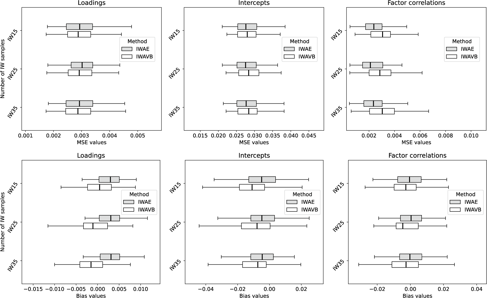
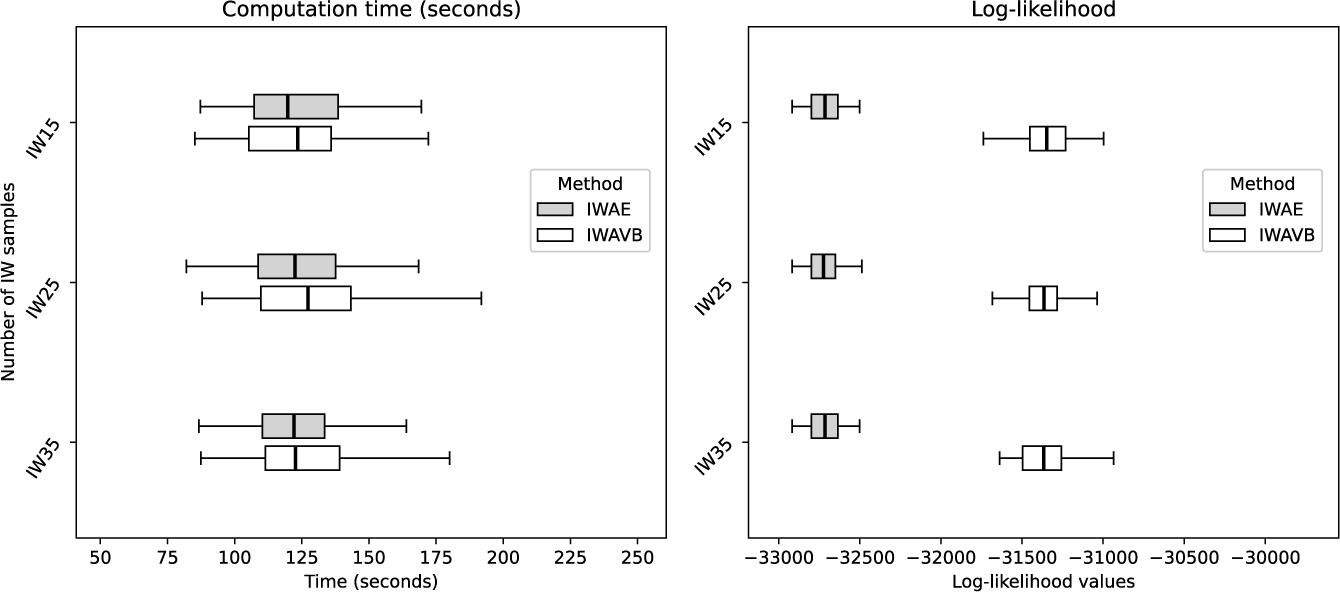
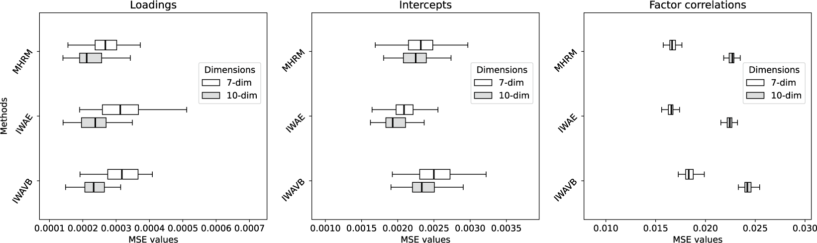
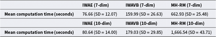
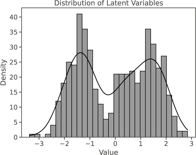
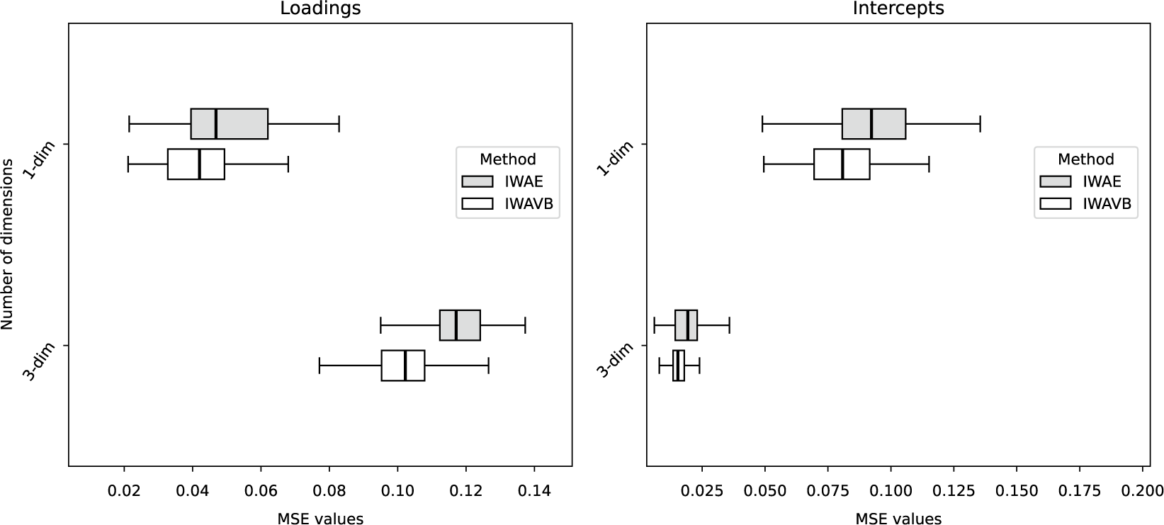
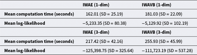
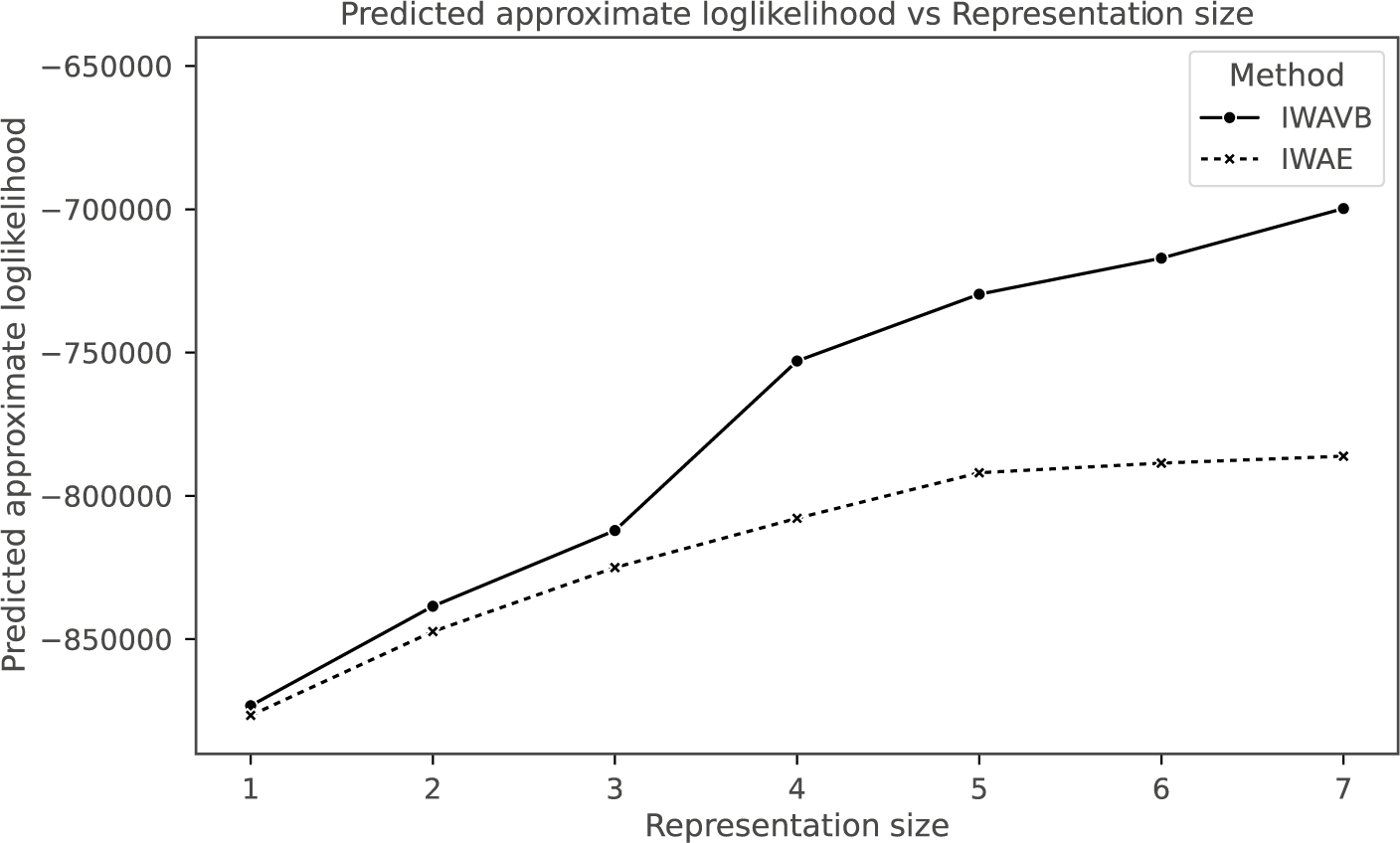
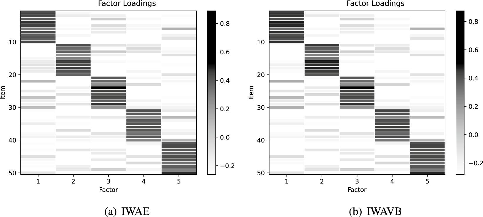
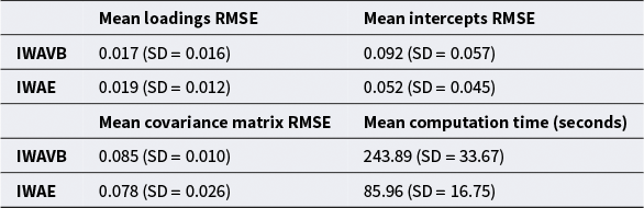

 Open access