Multivariate time series clustering analysis of the Global Dietary Database to uncover patterns in dietary trends (1990–2018)

Abstract

Objective:

Understanding country-level nutrition intake is crucial to global nutritional policies that aim to reduce disparities and relevant disease burdens. Still, there are limited numbers of studies using clustering techniques to analyse the recent Global Dietary Database (GDD). This study aims to extend an existing multivariate time series (MTS) clustering algorithm to allow for greater customisability and provide the first cluster analysis of the GDD to explore temporal trends in country-level nutrition profiles (1990–2018).

Design:

Trends in sugar-sweetened beverage intake and nutritional deficiency were explored using the newly developed programme ‘MTSclust’. Time series clustering algorithms are different from simple clustering approaches in their ability to appreciate temporal elements.

Setting:

Nutritional and demographical data from 176 countries were analysed from the GDD.

Participants:

Population representative samples of the 176 in the GDD.

Results:

In a three-class test specific to the domain, the MTSclust programme achieved a mean accuracy of 71·5 % (adjusted Rand Index [ARI] = 0·381) while the mean accuracy of a popular algorithm, DTWclust, was 58 % (ARI = 0·224). The clustering of nutritional deficiency and sugar-sweetened beverage intake identified several common trends among countries and found that these did not change by demographics. MTS clustering demonstrated a global convergence towards a Western diet.

Conclusion:

While global nutrition trends are associated with geography, demographic variables such as sex and age are less influential to the trends of certain nutrition intake. The literature could be further supplemented by applying outcome-guided methods to explore how these trends link to disease burdens.

Understanding the patterns of nutrition intake is important in providing evidence for stakeholders to develop appropriate policies for reducing associated disease burdens and disparities. While individual-level nutritional data analyses provide information about the impact on individuals’ health outcomes, country-level longitudinal data could provide a more in-depth understanding of how country characteristics, such as economic, cultural and geographical differences, relate to the observed trends in nutritional profiles.

However, country-level nutritional databases are made up of numerous nutritional variables and can therefore be extremely complex for interpretation. As such exploratory analyses can help individual governments or global health policy groups identify factors influential to existing disparities or disease burdens, or even encourage further ‘policy learning’^(1,2) and exchange of strategies between countries undergoing similar trends. A recent study⁽³⁾ explores worldwide multivariate dietary patterns by taking median values of time series, which almost completely disregards the temporal trends, while other studies that investigated country-level intake trends were limited to a single country⁽⁴⁾, a single nutritional variable⁽⁵⁾ or even a single nutritional variable within a single country⁽⁶⁾. Azzam et al.⁽⁷⁾ perform an exploratory analysis of data from food balance sheets to test whether there is a global convergence towards a Western diet, and they identify sixteen countries with consumption consistent with this. Their study collated consumption data into an index at each time point, and future studies could attempt to explore these trends over time in a time series manner. These examples highlight the gap in analysing longitudinal data from multiple countries.

There are vast amounts of data on nutritional intake, and to fully appreciate such data, computational and statistical methods are necessitated: clustering is a computational technique that could provide novel insights as to how nutritional profiles have evolved and identify groups of countries with similar intake trends or those that have trends distinct from any others. Longitudinal profiles could be analysed by directly applying standard clustering algorithms such as K-means⁽⁸⁾ or DBSCAN⁽⁹⁾ to snapshots of the data in a cross-sectional manner. Clustering is a form of unsupervised machine learning. Unsupervised machine learning involves analysing and grouping data without predefined labels, identifying hidden patterns or structures within the dataset. However, these standard clustering approaches would fail to leverage the temporal aspect available in nutritional datasets.

Multivariate time series (MTS) clustering is an unsupervised machine-learning method used to determine natural clusters of time series data. Unlike univariate time series clustering, this technique presents an attractive opportunity to extract value from multiple time series variables at once. More details regarding MTS clustering will be provided in the Literature Review section. MTS clustering was leveraged in a study of European countries with the aim of identifying similar consumption trends and a general dietary convergence⁽¹⁰⁾. However, their findings were limited due to the use of food balance sheets, which only capture a limited specificity of foods. In recent years, the Global Dietary Database (GDD) was developed, combining thousands of existing individual-level surveys to offer estimates of forty-seven intake variables between 1990 and 2018 for 188 countries. While this is a potentially extremely rich dataset for understanding how worldwide country-level intakes have evolved, no clustering technique, let alone MTS clustering, has yet been applied to the GDD. In addition, a study has pointed out that nutrition intake might be affected by the country level⁽¹¹⁾, but this finding has yet to be investigated using clustering techniques.

The nature of this paper’s methods appreciates the full temporal aspect of longitudinal data to capture trends over time. The novelty of this study is the application of these MTS clustering methods to the data-rich GDD. While this work is exploratory in nature, the findings may be of interest to global health governance, particularly for organisations like the WHO, in formulating region-specific nutrition policies and tracking progress towards global nutrition targets. Ultimately, this research contributes to a deeper understanding of global nutritional trends and further exploring these trends could pave the way for more effective strategies and nutrition policies to improve population health.

Aim

Considering the small number of available literatures on MTS clustering of nutritional profiles and the potential impact of findings in nutritional intake trends on global health policies, it is crucial that MTS clustering techniques must be applied to a more comprehensive database for identifying nutritional intake trends at the country level. To achieve this goal, this study will first develop a MTS clustering programme (‘MTSclust’) which extends an existing approach (‘DTWclust’)⁽¹²⁾ but is generalised to use any distance metric and modified for further customisability. The first aim is to assess the performance of this newly developed programme and compare it to another time series clustering algorithm.

The second aim is to explore trends in country-level nutritional profiles between 1990 and 2018 using two different clustering perspectives. In the first approach, MTSclust is applied in a bivariate manner to identify groups of countries with similar trends in sugar-sweetened beverage intake and nutritional deficiencies to understand whether these trends differ by demographics. In the second approach, MTSclust is applied in a high-dimensional manner with around fifty nutritional variables being included to generate a ‘World Nutrition Intake Trend Classification’ to identify groups of countries with similar nutritional profiles.

Literature review

Time series distance metrics

To compare any two time series, one can utilise a distance metric. There are several existing metrics, and these can be referred to as ‘similarity’ and ‘dissimilarity’ metrics although one must take care to invert the output depending on the use case⁽¹³⁾. The most basic cases include Euclidean distance, the popular Dynamic Time-Warping distance and the temporal correlation (CORT) dissimilarity⁽¹⁴⁾.

The Euclidean distance between two univariate time series, ${{\boldsymbol{X}}_T}$ and ${{\boldsymbol{Y}}_T}$ (both of length $m$ ), assumes a one-to-one mapping of points. It captures similarities in time series that directly overlap. Therefore, if ${{\boldsymbol{X}}_T}$ and ${{\boldsymbol{Y}}_T}$ contain identical trends but have a large time off-set, they would not be identified as similar. Z-score normalisation (standardisation) could be applied to the time series beforehand if the impact of magnitude is not of interest. The $i$ ^th point in one time series is compared to the $i$ ^th point of the other:

$${d_{EUCL}}\left( {{{\boldsymbol{X}}_T},{{\boldsymbol{Y}}_T}} \right) = \sqrt {\mathop \sum \limits_{i\,=\,1}^m {{\left( {{X_i} - {Y_i}} \right)}^2}}\;.$$

In contrast, dynamic time warping (DTW) distance can capture the similarity of trends that are offset (differing start and end) and of varying speeds (differing lengths of time or ‘skewed’). For the coupled observations ( ${X_{{a_i}}}$ , ${Y_{{b_i}}}$ ), DTW finds a mapping of the time series, $r$ , so that the distance between them is minimised while ${\boldsymbol{M}}$ is the set of all admissible sequences of $m$ index pairs of observations that (1) the beginning and end of the two time series are matched together, and (2) the sequence is monotonically increasing with all time series indexes appearing at least once:

$${d_{{\rm{DTW}}}}\left( {{{\boldsymbol{X}}_T},{{\boldsymbol{Y}}_T}} \right) = \mathop {\min }\limits_{r \in M} \left( {\mathop \sum \nolimits_{i\,=\,1}^m \left| {{X_{{a_i}}} - {Y_{{b_i}}}} \right|} \right)\;.$$

Another dissimilarity index is CORT⁽¹⁴⁾. This index incorporates time series raw value proximity as well as their temporal correlation behaviours. More details, including the formulae, are provided in the online supplementary material, Supplemental 1.

Dimension reduction

‘Curse of Dimensionality’ is one of the challenges that one might face when using machine learning approaches to analyse high-dimensional data⁽¹⁵⁾. For example, the K-means distance-based measure converges as the number of dimensions increases, which makes it less effective at distinguishing points. The aim of dimension reduction is to represent the data in a lower dimensional space whilst minimising information loss and further avoiding the ‘Curse of Dimensionality’⁽¹⁶⁾. However, this approach is also limited by the fact that multiple projections to a lower-dimensional space exist, and these sub-spaces could potentially have different clustering results. In this study, the dimensionality of MTS can refer to either the number of nutritional variables or the length of time series.

The simplest approach to dimension reduction is ‘Feature Selection’, which refers to the removal of unnecessary variables based on existing knowledge or statistical considerations⁽¹⁶⁾. Another common approach to reducing variables is principal component analysis, which transforms correlated variables into uncorrelated variables by projecting the original data onto the space spanned by the eigenvectors of the variables’ correlation matrix⁽¹⁷⁾.

To reduce the lengths of time series, segmentation can be utilised to extract the most distinguishing periods of a time series. It is useful for time series with long spans of inactivity⁽¹⁸⁾. Sliding window approaches can be adapted to reduce the resolution of time series. A similar outcome can be achieved using piecewise linear approximation. One could also represent the data using transformations such as the discrete wavelet or Fourier⁽¹⁹⁾ transformations which attempt to decompose features of the time series. In addition, clustering very large time series by extracting global characteristics, such as trend, seasonality, periodicity and serial correlation, is another strategy⁽¹⁸⁾.

Approaches

MTS clustering algorithms are often designed by combining time series distance metrics and dimension reduction. Regarding the application of DTW for MTS, an R package ‘DTWclust’ provides an implementation but failed to clearly state how it handles the multivariate case⁽²⁰⁾. Another DTW implementation written in Python handles the multivariate case by simply concatenating the variables into a univariate time series⁽²¹⁾. Given that DTW identifies similarities in two time series even if they are offset, the concatenation of variables in such a manner could therefore result in trends from different variables being accidentally matched.

On the other hand, a recently developed MTS clustering approach utilises common principal component analysis, which is a variation of principal component analysis assuming that multiple datasets share principal components, to represent the data in a lower dimensional space before clustering with K-mean⁽²²⁾. However, package source code was not provided, complicating the replication of their algorithm and performance tests. Meanwhile, spectral clustering utilises eigenvalues of variable similarities to perform dimensionality reduction before clustering, and a variation of this algorithm has been developed for time series although not for multivariate time series⁽²³⁾.

Furthermore, there have been recent developments in deep-learning approaches for MTS clustering⁽²⁴⁾. Many of these models can be considered ‘black-box’ models, meaning their decision-making to create outputs (clustering results) is not easily understandable. These models are more difficult to interpret. In many clustering applications, it is important to know what metrics are determining the outcome, especially given that clustering can be considered somewhat of an art, not an exact science⁽²⁵⁾.

One example of a recent deep-learning MTS approach is to utilise a variational AutoEncoder architecture to compress multiple time series variables into a single dimension for hierarchical clustering⁽²⁶⁾. In this case, interpretability may be difficult as it may not be clear which elements of the different time series variables are retained in the single-dimension representation. Variational AutoEncoders are a type of neural network architecture designed for unsupervised machine learning, particularly effective in dimensionality reduction and generative tasks⁽²⁷⁾. The encoder maps high-dimensional data (such as several nutritional variables) into a lower-dimensional space.

In most of the above cases, the target number of clusters is required. This can be guided by the intended use case, or via heuristics such as the Elbow, Silhouette or Gap method⁽²⁸⁾. Overall, the literature on MTS clustering is quickly evolving, but the reproducibility remains to be examined^(22,29) .

Evaluating clustering performance

Whilst there are several existing strategies to evaluate standard clustering algorithms, approaches specific to MTS are limited⁽³⁰⁾. Most clustering algorithms aim to output cluster assignments, and hence, the same performance metrics can be used, but complications arise when attempting to define the specific task to be evaluated: many of these algorithms are domain dependent so whilst evaluating using existing benchmarks may be the simplest approach, the same performance may not be observed when applied to the domain of interest⁽³⁰⁾.

Clustering algorithms aim to group observations based on their similarity. In most cases, clustering is applied to unlabelled data where no predefined categories or ‘ground truth’ labels exist, making it a purely unsupervised machine learning task. However, when labels are available, such as in datasets where the true class of each observation is known, clustering results can be evaluated in comparison to these labels. In such cases, the Rand Index (RI) is a metric that can be applied to evaluate clustering results. This metric is similar to accuracy and can be thought of as a measure of the proportion of correct assignments⁽³¹⁾. It can be computed as follows where TP, FN, FN, and TN are the numbers of true positive, false positives, false negatives and true negatives:

$${\rm{RI}} = {{\rm{\;}}{{{\rm{TP\;}} + {\rm{\;TN}}}}\over{{{\rm{TP\;}} + {\rm{\;FP\;}} + {\rm{\;FN\;}} + {\rm{\;TN}}}}}.$$

The adjusted Rand Index (ARI) is similar to the Rand Index but corrects for chance, which can make it a more appropriate evaluation metric. An ARI of 0 suggests clustering outputs are similar to random selection while an ARI close to 1 suggests the clustering outputs are better than random selection. A value below 0 suggests clustering outputs are worse than random selection. The formula for ARI can be found in the online supplementary material, Supplemental 1.

Methods

Data

Global Dietary Database

The GDD⁽³²⁾ includes country-level nutritional data from 1990 to 2015 at 5-year intervals (1990, 1995, 2000, 2005, 2010, 2015) and the data of 2018. In this database, forty-seven nutritional variables, which include thirteen macronutrients, eighteen micronutrients, five beverages and eleven foods, are available. In terms of demographic information, age, sex, education and urbanisation are provided. In this study, only age and sex were included in the analyses.

Nutritional deficiency

Disability-adjusted life years lost caused by nutritional deficiency were obtained from the Global Burden of Diseases Study⁽³³⁾. Each unit of disability-adjusted life years indicates 1 year of full health loss as a result of premature mortality and years lived with the disability. Data on disability-adjusted life years were available for all years between 1990 and 2019, for all countries of interest. This variable was sourced from various existing datasets and primary data collections, such as disease registries and household surveys. A disease meta-regression model is used to generate the estimates⁽³⁴⁾.

Income classifications

Historical income classifications between 1990 and 2018 are provided by the World Bank⁽³⁵⁾. For each year, countries are classified into one of four groups: (1) low income, (2) lower middle income, (3) upper middle income and (4) high income based on gross national income (GNI) per capita, in U.S. dollars. GNI is estimated by economists, and population size is estimated by the World Bank.

Data pre-processing

The GDD uses various data sources to generate estimated nutrition intakes; hence, it was complete and did not require further data imputation. Data for nutritional deficiency were obtained from a separate dataset: the Global Burden of Diseases Study⁽³³⁾. To ensure both datasets were in a compatible format, nutritional deficiency observations were dropped to match the years of interest as indicated in the GDD (retained years: 1990, 1995, 2000, 2005, 2010, 2015 and 2018). For income classifications, after extracting the years of interest, countries with one missing value were imputed by simply using the most recent value from other years (e.g. if 1990 was missing, then 1991 was used, not 1995).

Notably, since income classifications are time-dependent variables, to simplify the interpretability, countries that were originally labelled as lower middle income or upper middle income were first merged into a new middle income. Based on the income trends, countries were then classified into six groups: (1) constantly low income, (2) constantly middle income, (3) constantly high income, (4) increasing then decreasing income trend, (5) decreasing income trend and (6) increasing income trend. Because groups 4 and 5 have low sizes and would unnecessarily complicate the interpretation of the clustering performance, countries there were in either group 4 or 5 were removed. The final dataset comprised 176 countries.

Programme development

MTSclust algorithm

To address the first aim a newly implemented programme, ‘MTSclust’, was developed based on the DTW multivariate time series clustering algorithm⁽¹²⁾. The key difference is generalisation to allow for the use of any distance measure. MTSclust calculates dissimilarities in the univariate time series space and aggregates these into a single matrix which can be analysed by several standard (non-time series) clustering algorithms⁽³⁶⁾, which is a common technique for developing clustering algorithms and is similar to existing approaches^(37–39). Algorithm 1 provides the pseudo-code.

Algorithm 1: MTSclust

Inputs: Multivariate time series for N number of items; K target number of clusters

Output: Cluster assignments for N items

1. Initiate empty N × N matrix

2. For each time-series variable do

i. Calculate time series dissimilarity

ii. Add dissimilarity to the existing N × N matrix (optionally weighted)

3. Perform clustering on the N × N aggregated dissimilarity matrix from above, (e.g. using hierarchical or PAM; or optionally mapped to Cartesian space with MDS)

The time series dissimilarity matrix can be calculated using one of many existing measures such as the Euclidean, DTW, compression-based, correlation-based or partial autocorrelation metric⁽³⁷⁾. As discussed in the previous section, distance metric selection is highly dependent on use case⁽¹³⁾. In our study, the CORT distance metric would be an appropriate metric because it captures similarities in both temporal correlation behaviour and raw value proximity. Other potentially applicable distance metrics include CDM, DTWARP, EUCL and NCD, which are all provided in the TSclust R package⁽⁴⁰⁾.

It is crucial to highlight that not all sub-clustering algorithms are immediately compatible: for example, the K-means clustering algorithm⁽⁸⁾ processes Cartesian coordinates rather than a dissimilarity (distance) matrix. To use K-means, one could map the aggregated dissimilarity matrix to an abstract 2D space using a multidimensional scaling (MDS) algorithm, such as non-metric MDS⁽⁴¹⁾. MDS is a form of non-linear dimensionality reduction, and information loss is likely to happen⁽⁴²⁾. It is important to retain as much information as possible, hence why Hierarchical and PAM are used for sub-clustering in this study. The MTSclust programme allows for the weighting of particular time series variables, which could be used to prevent a variable of interest from being ‘drowned out’, an important consideration when dealing with high-dimensional multivariate data.

Performance comparison

For comparison, MTSclust was benchmarked against a popular algorithm ‘DTWclust’. Trends in income levels, which were defined based on World Bank Income Classifications, were selected as the labels to assess the performance of these algorithms. In addition, nutritional variables known to be correlated with income, including nutritional deficiency, sugar-sweetened beverages, added sugar, iodine, vitamin A and zinc, were selected as inputs. Three different test sets of income trends were utilised for the performance analysis: (1) low-income v. high-income, (2) low-income v. middle-income v. high-income and (3) low-income v. increasing income. The tests, which aim to differentiate countries by these trends, were repeated 1000 times for each variable, and the median accuracy for each algorithm was reported.

To evaluate the cluster performance, four measurements: accuracy (%), run-time (seconds), Rand Index and ARI were included in the performance metrics. The arbitrary cluster IDs had to be remapped to the known labels to obtain these metrics. A snippet of R code was developed for this project to find the optimal remapping by comparing the accuracy of all possible permutations of labels, allowing one to obtain performance metrics from cluster assignments.

Reference values were generated based on 1000 simulated randomised repeats of a dummy clustering algorithm. Such reference values would allow one to gain an understanding of how much better the clustering algorithms are than randomness, similar to the adjusted Rand Index.

Applying multivariate time series clustering algorithm to Global Dietary Database

To satisfy the second aim of this study, trends in sugar-sweetened beverage intake and nutritional deficiencies were explored. MTSclust was applied to the two variables using the CORT distance metric. This metric captures both Euclidean and temporal similarities in time series. The target number of clusters was defined as 4 (K = 4) to strike a balance between having too many clusters that complicate the interpretation and having too few that the respective clusters do not contain a common trend. The trends in generated clusters were then visually explored. Demographic-specific trends were explored by repeating the above using the stratified GDD data (sex and age).

In addition, trends in all nutritional variables were explored with MTSclust being applied to all forty-seven GDD intake variables plus the nutritional deficiency variable. Variables were equally weighted, and the CORT distance metric was used. The resultant cluster assignments could be loosely described as a ‘World Nutrition Intake Trend Classification’. This was created for four groups of countries (K = 4) and six groups of countries (K = 6) respectively.

Software

Data processing scripts were originally written in Python (using Google Colab, an online notebook lab space) as this can make use of powerful libraries such as Pandas for quick data wrangling of large datasets. The analysis stages were written in R as most of the key packages, such as DTWclust⁽²⁰⁾ and TSclust⁽⁴⁰⁾, were written in this language. Eventually, the data processing Python scripts were converted to R to increase interoperability with the analysis stages. Having a single codebase also makes it easier for other researchers to reproduce the analysis. A link to the GitHub code repository to reproduce this analysis is provided in online supplementary material, Supplemental 2. The ‘MTSclust’ programme is provided as an R package within the code files.

Application

Clustering performance comparison

Tuning DTWclust

Prior to comparing performance, DTWclust was tuned using a tune grid to find the optimal combination of parameters. Figure 1 demonstrates the performance of the sixteen combinations after each combination ran 1000 repeats with different seeds. The combinations were defined based on four parameters: (1) Manhattan distance or Euclidean distance, (2) distance being square rooted or not, (3) backtracking technique being applied or not and (4) data being normalised or not. In this violin plot, the red points indicate median accuracy for each set of 1000 runs with the values ranging from 0·694 to 0·748.

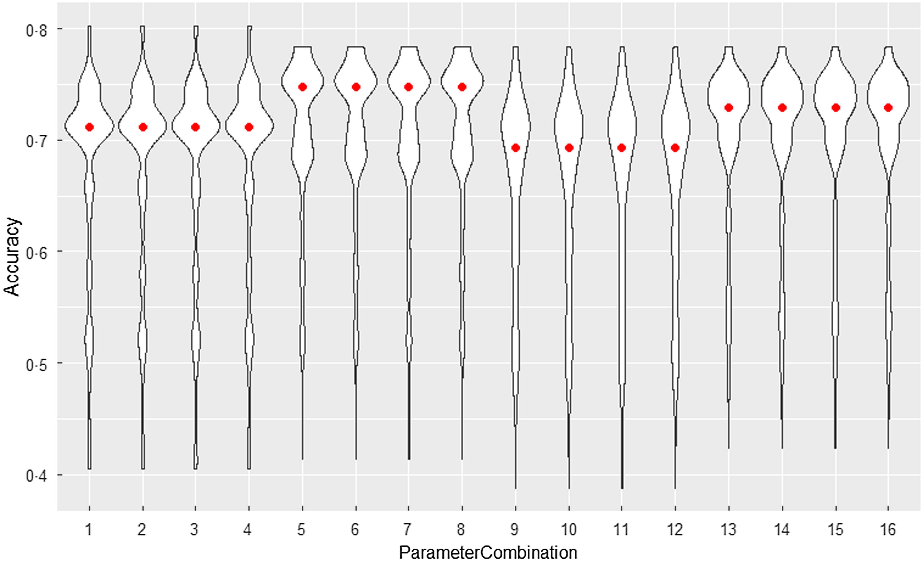
Figure 1. Violin plots for DTWclust tuning repeats.

The optimal parameter setting (combination 5) was to use the square-rooted Manhattan distance for the local cost matrix of DTW. As observed, the combinations in the violin plot appear to be in groups of four. This is because normalisation and backtracking had no effect and were therefore not applied.

Performance comparison

To assess how well MTSclust and DTWclust were able to partition countries into their income levels based on the five closely correlated nutrition variables (sugar-sweetened beverage, added sugar, iodine, Zn and vitamin A intake), each of these five bivariate sets of variables was clustered 1000 times. As described earlier, three different test sets of income trends were utilised. In addition, for the first test sets, the process was repeated across the male and female GDD datasets to ensure robustness. The results are summarised in Table 1.

Table 1. Performance on clustering with different numbers of classes

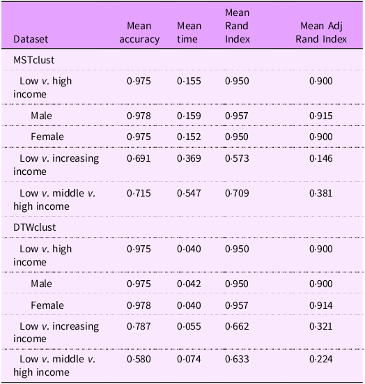
The performance analysis found that MTSclust in general performed better than ‘DTWclust’ in the three-class performance test with MTSclust achieving a mean accuracy of 71·5 % (ARI = 0·381) whereas DTWclust achieving 58·0 % (ARI = 0·224). Both algorithms performed well in two-class performance tests using high- and low-income class countries, both achieving 97·5 % (ARI = 0·90). In all test cases, MTSclust well exceeds the reference values. MTSclust is much slower: in the two-class test, it took on average 0·37 s, 3·88 times longer than DTWclust.

Results of applying multivariate time series clustering algorithm to Global Dietary Database

After validating the performance of MTSclust, this programme was then applied in a real-world setting. Clustering is first performed on two time series variables, which is also known as bivariate clustering. This is followed by an exploration of clustering on all forty-eight variables at once, known as the high-dimensional MTS clustering.

In the bivariate time-series clustering, sugar-sweetened beverage intake and nutritional deficiency were input variables for the clustering. ‘PAM’ and ‘CORT’ were used as the sub-clustering algorithm and the distance metric in MTSclust. In Figure 2, countries with similar trends in sugar-sweetened beverage intake and nutritional deficiency are clustered together. The clusters are loosely correlated with geography: Cluster 1 largely contains Latin American, Middle East and Southern Mediterranean countries; Cluster 2 largely contains South East Asian and Central African countries; Cluster 3 is ambiguous with countries scattered over several continents and Cluster 4 contains Western countries and the former Soviet region. It’s fair to say these clusters are not fully described by geography.

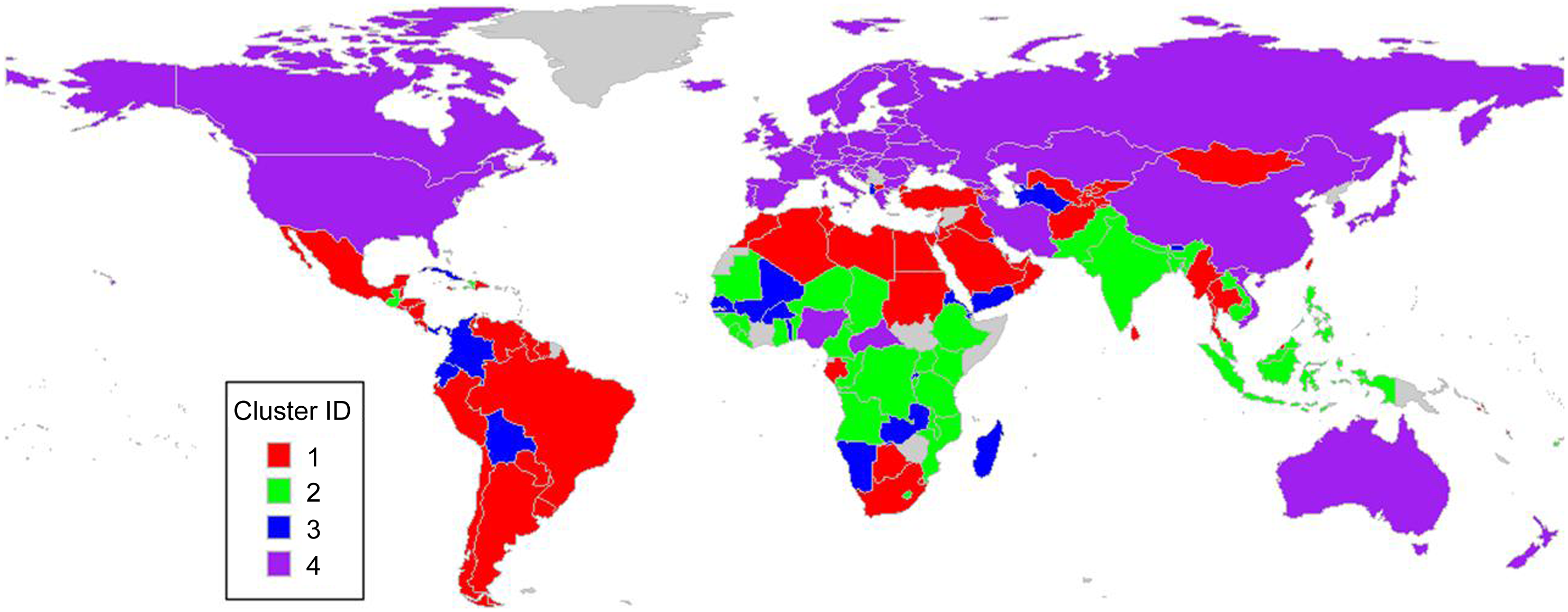
Figure 2. Map of bivariate clustering results (MTSclust).

To better understand the trends, the time series plots with each country coloured as per their cluster assignment are provided in Figure 3. In addition, given that the demographic-specific trends are also of interest, the datasets were stratified according to sex or age for analyses. The results demonstrated that some clusters are visually separable (see for example Cluster 3), but others are not (Figure 3(a) and (b)). This bivariate time series clustering identified four distinguishing trends among countries, as seen in these figures: Cluster 1 contained countries with increasing sugar-sweetened beverage intake whilst deficiency decreased. Cluster 2 contained countries with slightly increasing sugar-sweetened beverage intake and a steep decline in deficiency. Cluster 3 contained countries with highly erratic (and often very high) sugar-sweetened beverage intake whilst deficiency decreased. This erratic trend could be caused by the origin of the data: these are countries with small populations and in turn, a lower sample size which would increase the variation of estimates. Cluster 4 contained countries with constantly low sugar-sweetened beverage intake and low deficiency. These are largely developed countries in the northern hemisphere.

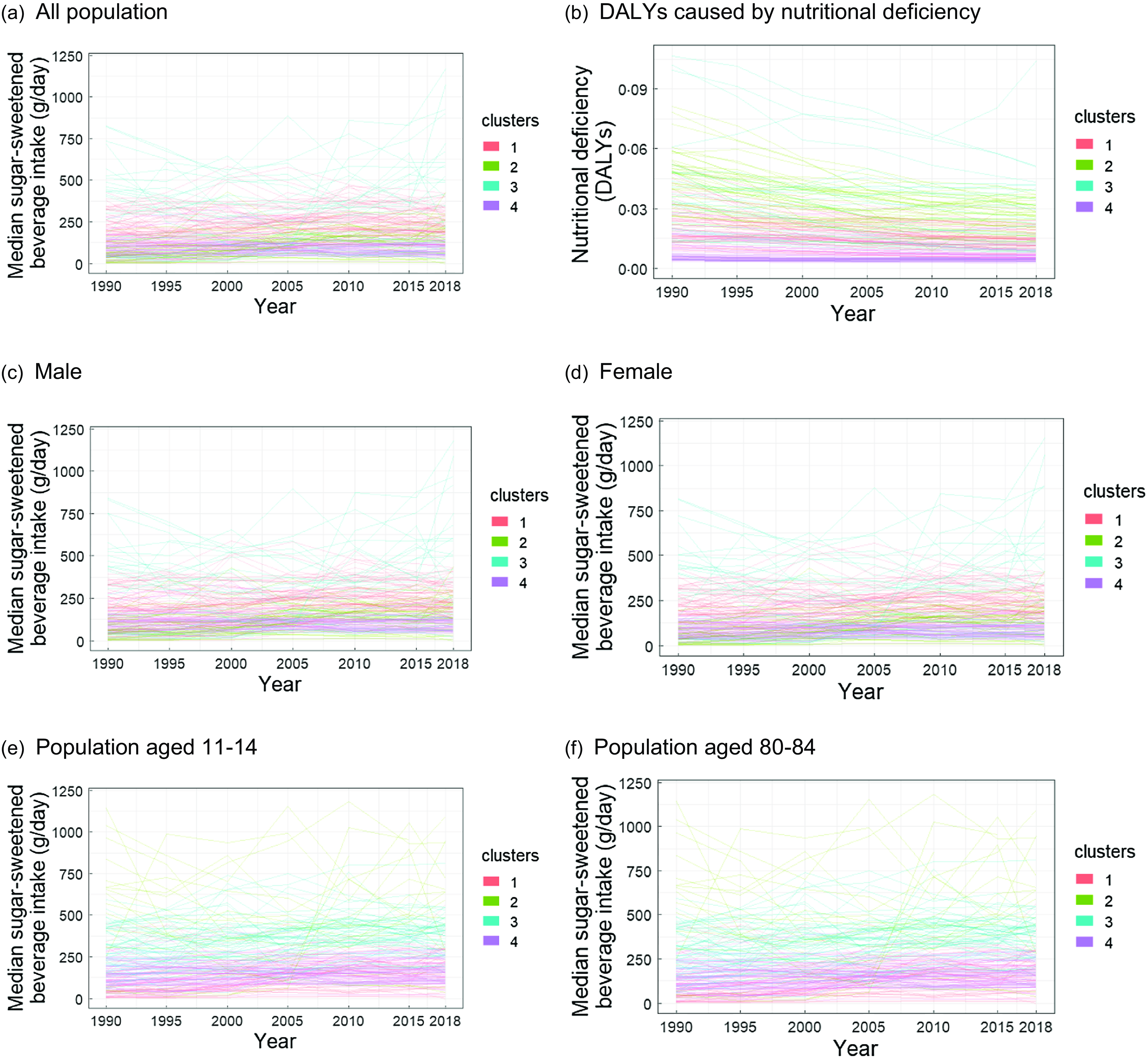
Figure 3. Time series plots of median sugar-sweetened beverage intake.

The methods identified no demographic-specific trends in these two variables sugar-sweetened beverage intake and nutritional deficiency) (Figure 3(c)–(f)). It could be said that these country-level trends between 1990 and 2018 do not seem to be dominated by sex or age. However, this finding could actually be caused by issues arising from data provenance: the GDD is comprised of estimates generated from multilevel Bayesian multilevel framework and relies on covariate information to support countries and demographics with limited individual-level intake data. It is also possible that these demographic-specific trends simply do not exist: perhaps in the long term, these demographic groups do indeed closely follow their country’s trends. In all graphs within Figure 3, the extremes (such as the very low or high values) tend to be clustered together. This is consistent with the choice of distance metric, CORT, which incorporates both raw-value proximity and trend behaviours (additional CORT details and formulae provided in online supplementary material, Supplemental 1).

The next analysis explores inter-country similarity based on trends within their entire nutritional profile (1990–2018): MTSclust with the CORT distance metric is applied to all forty-eight nutritional variables. As the clustering is performed on all variables, one could describe the output as a ‘World Nutrition Intake Trend Classification’ (Figure 4). As the figures demonstrated, the generated cluster assignments from the high-dimensional MTS clustering are highly correlated with geography. This is even the case when increasing the number of target clusters to six. Furthermore, the groupings of the K = 6 result are almost all subsets of the K = 4 result, suggesting that the clustering is stable. Cluster IDs 4 and 6 in the respective classifications are identical. The members of these groups are Bulgaria, Djibouti, Estonia, Israel, Lebanon, Mongolia and Palestine. These countries are diverse in terms of economics and geography, so it is a surprising grouping. This finding could suggest these countries have nutritional intake trends that are disparate relative to others: potentially a cluster grouping of outliers. For Figure 4(b) (K = 6 clusters), the groupings of clusters can be loosely described by geography as follows: Cluster 1 is dominated by African and South East Asian countries; Cluster 2 is similar to Cluster 1 with African and South East Asian countries; Cluster 3 is largely composed of former Soviet countries; Cluster 4 contains several coastal countries from the mediterranean, as well Latin America and a few coastal East Asian countries; Cluster 5 contains Western countries (North America, Europe and Australia) and Cluster 6 is not visually correlated to geography as described above.

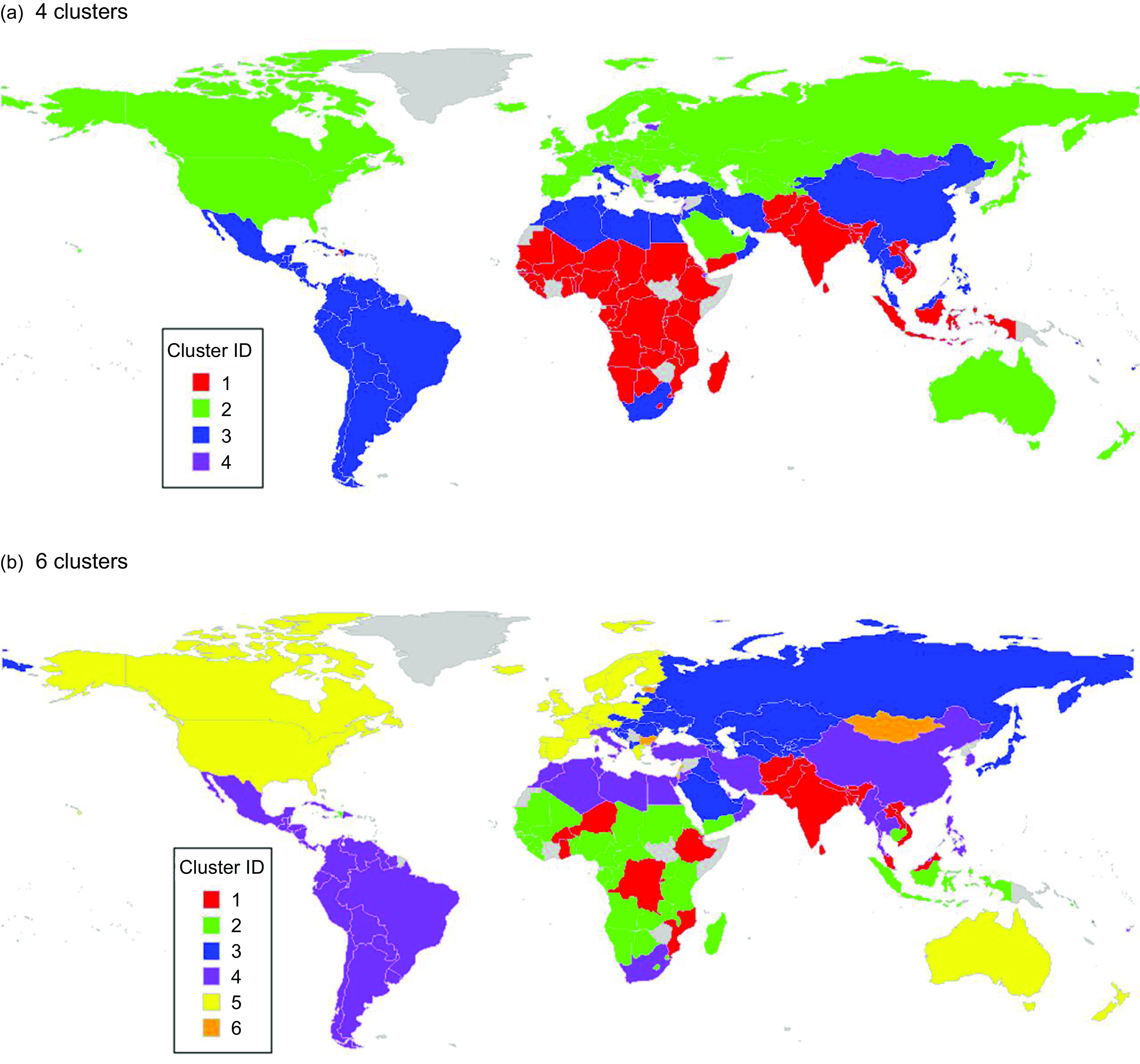
Figure 4. World Nutrition Intake Trend Classification by different numbers of clusters.

Discussion

This study investigated country-level nutritional trends and identified groups of countries with similar profiles using a variety of approaches including bivariate clustering and a high-dimensional approach. The bivariate time series clustering, based on nutritional deficiency and sugar-sweetened beverage intakes, identified four distinguishing trends among countries, but no demographic trend was identified. Whilst one can say that these country-level trends between 1990–2018 are not dominated by binary subgroups like sex or age, we should caveat that the lack of evidence to support them as potential effect modifiers could be due to insufficient statistical power. Future studies could attempt to perform a narrower and focused analysis of these particular country trends leveraging adequately powered analytical techniques such as regression analyses. On the other hand, the generated cluster assignments from the high-dimensional MTS clustering, which is the ‘World Nutrition Intake Trend Classification’, are highly correlated with geography. It is worth noticing that cluster IDs 4 and 6 in the respective classifications are almost identical, but they are diverse in terms of economics and geography, suggesting that this cluster is potentially a collection of countries with trends that are disparate relative to others. This finding therefore highlights the possible value in exploring clustering algorithms with outlier detection, such as DBSCAN and also K-value selection strategies.

Azzam et al.⁽⁷⁾ clustered consumption data from food balance sheets to test whether there is a global convergence towards a Western diet and they identified sixteen countries with consumption consistent with this. In contrast to our study, they explored food balance sheets and collated consumption data into an index at each time point. Despite this difference, all sixteen countries they identified were also grouped together in this project’s generated ‘World Nutrition Intake Trend Classification’ (Figure 4). In addition, this project identified a further thirty-four countries with similar trends (see Cluster 2 of Figure 4(a)). Similarly, almost all of the sixteen countries were also present in the K = 6 ‘World Nutrition Intake Trend Classification’, with the exception of Belgium, Czechia and Hungary (see ‘Cluster 5’ of Figure 4(b)).

Policy implications

The WHO classifies countries into six regions according to WHO’s planning, reporting and analysis needs⁽⁴³⁾. In a similar manner, the ‘World Nutrition Intake Trend Classification’, which was one of the outputs of this study, could potentially be used to subdivide regions for future nutrition-related policy, reporting and analysis. For instance, WHO specified six global nutrition targets for 2025 in 2012 and the United Nation listed zero hunger as one of the sustainable development goals (SDG) in 2015⁽⁴⁴⁾. While these global targets focus on nutrition, the relationship between economy and nutrition should also be investigated given that evidence has shown that countries with higher income levels had greater nutrition intake^(45,46) . The ‘World Nutrition Intake Trend Classification’ can, therefore, serve as an indicator to identify countries or regions with similar backgrounds for policy references and assessments. Regionalisation of nutrition policies in such a manner could help to ensure that interventions are tailored to the specific needs of different regions⁽⁴⁷⁾. Our findings demonstrate that nutritional patterns are not necessarily completely described by geographic location, so regionalisation defined by clustering may be a more targeted approach, recognising that nutritional challenges and patterns can vary substantially. Additionally, these methods could be utilised to support policy monitoring and evaluation: one could re-explore these subdivided regions in 10 years’ time, to potentially identify changes in countries between clusters, or larger structural shifts of the clusters. For the purpose of policy planning, one could also potentially use these clustering results to project trends into the near future. Regionalisation (facilitated by clustering) could allow for more efficient prioritisation of resources: by identifying regions with the most pressing nutritional needs or those where interventions are likely to have the greatest impact, policymakers can strategically allocate limited resources. Methods-wise, one could re-apply the MTS clustering on one of our clustering output sub-groups (such as Cluster 1 in Figure 4(a)) to try to granularly explore whether there are any unidentified differences within each cluster grouping.

Furthermore, one may also use the generated ‘World Nutrition Intake Trend Classification’ to support the creation of population health ‘policy learning networks’⁽⁴⁸⁾: countries undergoing similar trends in nutritional deficiency may benefit from sharing strategies and proposals to alleviate this. The entities that would benefit from such networks would be very niche, specifically, this would be of benefit to government bodies and non-governmental organisations (NGO) tackling nutritional deficiency and agricultural policy. These networks can facilitate the exchange of knowledge, experiences and best practices among countries facing similar nutritional challenges. By fostering collaboration and shared learning, policymakers can identify effective strategies and adapt them to their specific contexts. This can help to accelerate progress towards global nutrition targets. For instance, countries in the same cluster can share successful policies for reducing sugar-sweetened beverage consumption or improving access to a targeted nutritional intake variable. While this study focuses on novel applications of methodology, future studies could build upon these findings to perform more granular investigations into nutritional deficiencies in an outcome-guided manner.

Understanding global nutrition trends can be of interest to global health governance. By identifying groups of countries with similar nutritional profiles, policymakers can develop targeted interventions to improve nutrition and reduce disparities. For example, countries with high levels of sugar-sweetened beverage intake could implement policies to reduce consumption, such as taxes or marketing restrictions⁽⁴⁹⁾. Countries with high levels of nutritional deficiency could implement policies to improve access to nutritious foods, such as subsidies or education programmes.

Strengths and limitations

Regarding the developed clustering programme, a matrix of dissimilarities was created as part of the high-dimensional MTS cluster analysis, and one could convert this to Cartesian coordinates using MDS. This could potentially be used by future studies in a very specific case where one wishes to adjust for country-level nutrition intake trends. This adjustment helps to isolate the impact of specific interventions or policies on health, providing valuable insights for policymakers. For example, if researchers are studying the impact of a sugar-sweetened beverage tax on obesity rates, they could use the MDS matrix to adjust for the overall nutritional similarity between countries, ensuring that the observed effects are not simply due to pre-existing differences in dietary patterns.

This project presents the first cluster analysis of trends in the GDD. Other studies have analysed GDD trends although they are limited to single intake variables or particular countries⁽⁵⁰⁾. Specifically, this project leverages MTS clustering to ingest all forty-seven GDD intake variables in a single exploratory analysis. The newly developed programme, MTSclust, successfully identified intake trends against the backdrop of several nutritional studies which have failed to appreciate the temporal element of collected data^(7,10) . Moreover, this study conducted an analysis of nutritional profiles from two different perspectives, bivariate time series clustering and high-dimensional MTS clustering, allowing us to create a more comprehensive picture of nutrition trends. MTSclust and the accompanying analyses are thoroughly documented, enhancing the reproducibility of our findings. Furthermore, the design choice of MTSclust which leverages sub-clustering algorithms that can readily handle dissimilarity matrices, ensures less information is lost.

This study is not without limitations. The primary dataset (GDD) comprises purely country-level data; therefore, the scope of conclusions is immediately narrowed and is at risk of ecological fallacy, which refers to the error of making inferences about individuals using aggregate data. To draw further inferences about nutritional profiles and health outcomes, one should investigate at the individual level. A limitation of the MTSclust programme is that the variables are compartmented for the calculation of trend similarities. While this helps generate more interpretable trends, it misses out on identifying more complex intervariable trends. Multivariate time series clustering provides a promising opportunity to analyse high-dimensional datasets with numerous nutritional variables, uncovering hidden patterns in data which might otherwise be too complex to detect. These methods could be applied to datasets similar to the GDD: studies could explore similar types of nutrition data or even other global public health data. One could perform a more granular investigation of intra-country patterns of nutrition intake: for instance (with an appropriate dataset), one could attempt to explore how dietary patterns in British counties have evolved over time.

Conclusion

In this study, the newly developed MTSclust programme was applied to investigate global nutritional trends. The bivariate cluster analysis of sugar-sweetened beverage intake and nutritional deficiency successfully separated countries into four visually distinct groups of trends, although it did not identify any demographic-specific trends. The ‘World Nutritional Intake Classification’, generated through a high-dimensional cluster analysis, highlights how global nutritional trends (1990–2018) are closely related to geography.

In conclusion, this study can be the foundation for the application of outcome-guided clustering techniques to further investigate the links between nutritional profiles and health outcomes.