High-resolution spectral analysis of three high-latitude carbon stars

Abstract

We present the results of a detailed high-resolution spectroscopic analysis (SUBARU/HDS spectra, R$\sim$50 000) of three faint high-latitude carbon stars HE 1104$-$0957, HE 1205$-$0521, and HE 1244$-$3036. Our estimated metallicity for these objects is $-$2.96, $-$2.63, and $-$2.49, respectively. The surface chemical compositions of the objects are found to be characterised by enhanced carbon and heavy elements, such as Y, Ba, La, and Ce. Using the classification criteria for carbon-enhanced metal-poor (CEMP) stars the objects HE 1104$-$0957 and HE 1205$-$0521 could not be classified into any known CEMP sub-classes, whereas the object HE 1244$-$3036 is found to be likely a CEMP-s star. The observed abundance patterns in HE 1244$-$3036 are also found to match well with the yields of a 2 M$_{\odot}$ AGB star with [Fe/H] = $-$2.50. Although our kinematic analysis indicates that the objects belong to the halo population, the elemental abundance ratios of HE 1104$-$0957 and HE 1205$-$0521 do not match well with those of typical halo objects. Estimated elemental abundances are presented, and kinematic properties of the stars are discussed.

1. Introduction

The Galactic halo is one of the most primitive regions of the Milky Way galaxy and holds very old stellar populations that are as old as our Milky Way itself (Frebel 2018). The chemical compositions of Galactic halo stars can give insight into various stellar progenitors and help to better understand the nature of nucleosynthetic pathways at earlier times. These stars are believed to be formed from the remnants of the Population III stars and hence hold the fossil records of the nucleosynthesis products of the very first stars. Thus, the detailed surface chemical composition of these old halo stars can give insight into the early Galactic nucleosynthesis.

Many sky survey programs (Beers, Preston, & Shectman 1985, 1992; Beers 1999b,a; Wisotzki et al. 2000; Christlieb et al. 2001; De Silva et al. 2015; Majewski et al. 2017; Conroy et al. 2019; Buder et al. 2021; Cooper et al. 2023) were conducted to explore metal–poor stars in the Galactic halo. These surveys have shown that the fraction of metal–poor stars that show enhancement of carbon increases with decrease in metallicity (Cohen et al. 2005; Frebel et al. 2006; Carollo et al. 2012; Lee et al. 2013; Placco et al. 2014; Beers et al. 2017). These group of metal–poor stars that exhibit enhancement of carbon are called carbon–enhanced metal–poor (CEMP) stars.

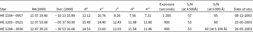
Table 1. Basic data of the programme stars.

$^{\ast}$ Simbad (2MASS survey Cutri et al. 2003)

CEMP stars comprise four primary subgroups: CEMP–s, CEMP–r/s, CEMP–r and CEMP–no (Beers & Christlieb 2005). Among these subgroups, CEMP–s stars are the metal–poor ([Fe/H] $\lt$ $-$ 1) counterparts of CH stars that are characterised by strong CH bands in their spectra. These stars exhibit enhancement of carbon and s–process elements. CEMP–r/s stars exhibit enhancement of both r– and s–process elements, CEMP–r stars show enhancement of r–process elements and CEMP–no stars do not show enhancement of heavy elements. The evolutionary states to which CH, CEMP–s and CEMP–r/s stars belong do not support the enhancement of carbon and other heavy elements observed in these stars. Many studies have shown that most of these stars exhibit radial velocity variations and are probably in binary systems (McClure & Woodsworth 1990; Preston & Sneden 2001; Hansen et al. 2016b; Jorissen et al. 2016). As per this concept, these stars might have accreted the nucleosynthesis products produced by their companion during their asymptotic giant branch (AGB) phase. In the course of studies on CH, CEMP–s, and CEMP–r/s stars, we have found observational evidence for AGB mass transfer for several of these objects (Purandardas & Goswami 2021; Goswami, Rathour, & Goswami 2021a; Shejeelammal & Goswami 2022). Continuing with these studies, in this work, we have presented results from high–resolution spectroscopic analysis of three faint high–latitude carbon stars that are potential metal–poor star candidates. Only limited studies are available for our programme stars (Koen & Eyer 2002; Goswami 2005; Beers et al. 2007; Limberg et al. 2021). We present for the first time a detailed high–resolution abundance analysis for these objects. We have presented the abundance analysis results for HE 1104 $-$ 0957 and HE 1244 $-$ 3036 using high–resolution spectra in Purandardas, Goswami, & Rengasamy (2024) and Dutta & Goswami (2024). In this work, we have scrutinised the potential progenitors of these objects using estimated elemental abundance ratios. Additionally, we have derived the orbital parameters, spatial velocity, galactic membership probabilities, and accretion histories while also checking the possibility of any internal mixing in these stars.

The paper is organised as follows: Observations and data reduction are presented in Section 2. Photometric temperatures of these objects are briefly discussed in Section 3, and in Section 4, we have discussed the estimation of stellar atmospheric parameters, including mass and age estimates. Section 5 presents abundance analysis and abundance uncertainties are discussed in Section 6. In Section 7, we present a detailed discussion on the abundance results and the kinematic analysis of the objects is presented in Section 8. Section 9 presents a discussion on the orbital properties and potential association of the programme stars with the Galactic Substructures. Some concluding remarks are presented in Section 10.

2. Observations and data reduction

The objects are selected from the list of faint high latitude carbon stars of Christlieb et al. (2001). The high–resolution spectra ( $R\sim 50 000)$ of the programme stars are acquired from the Japanese Virtual Observatory (JVO) portal http://jvo.nao.ac.jp/portal/v2/) operated by the National Astronomical Observatory of Japan (NAOJ), which provides reduced and wavelength–calibrated spectra. These spectra that are publicly available were obtained using the High Dispersion Spectrograph (HDS) of the 8.2 m Subaru Telescope. The spectra of HE 1104 $-$ 0957 and HE 1205 $-$ 0521 cover a wavelength range that extends from 4100 to 6850 Å. There exists a gap between 5440 and 5520 Å, which arises from the physical separation between the two EEV CCDs with 2 048 $\times$ 4 096 pixels with two by two on–chip binning. The wavelength coverage of the spectrum of HE 1244 $-$ 3036 is from 3510 to 5310 Å. Basic data of the programme stars are presented in Table 1. A few sample spectra of the programme stars are shown in Fig. 1 as examples.

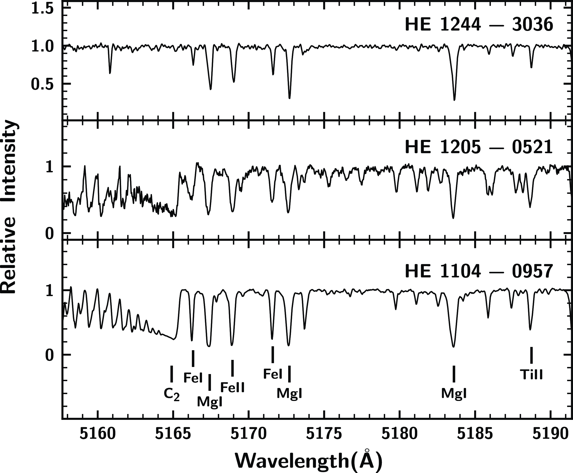
Figure 1. Sample spectra of the three programme stars in the wavelength region 5158–5191 Å are shown. Some features identified are marked on the spectra.

3. Photometric temperatures

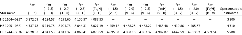
The photometric temperatures of the programme stars are derived using the calibration equations provided by Alonso, Arribas, & Martinez–Roger (1999). We have followed the same procedure as described in Goswami et al. (2006), Goswami, Aoki, & Karinkuzhi (2016) and Goswami, Rathour, & Goswami (2021a). This calibration equation connects $T_{\rm eff}$ with colours and metallicity of the star. The precision of the fits ranges from 40 K for (V–K) to 170 K for (J–H). The J, H, and K magnitudes of the programme stars are taken from 2MASS survey (Cutri et al. 2003). The photometric temperatures derived using the calibration equations of Alonso, Arribas, & Martinez–Roger (1999) for our programme stars are presented in Table 2.

We have also estimated the photometric temperatures of our programme stars using the Gaia photometry (Table 3). We have used the colour– $T_{\rm eff}$ calibration equation from Mucciarelli, Bellazzini, & Massari (2021) for estimating the temperature. The $T_{\rm eff}$ obtained this way has a typical dispersion of around 40–80 K for giants. Mucciarelli, Bellazzini, & Massari (2021) also noted that (BP–RP) should be preferred over other GAIA magnitude combinations, as the effects of contamination from unrelated light sources in the BP and RP bands tend to cancel out when subtracted. We have compared both the photometric temperatures with our spectroscopic estimates for each of the programme stars. We could see that the $T_{\rm eff}$ derived using the colours (J–K), and (BP–RP) match quite closely to the spectroscopic estimate in the case of HE 1104 $-$ 0957, i.e., the estimated spectroscopic temperature is 72 K higher than the 2MASS photometric temperature and 17 K higher than the Gaia (BP–RP) temperature. These differences lie well within the margin of errors. In the case of HE 1205–0521, we noticed that the estimated 2MASS and Gaia temperatures differ by about 329 K, and this difference is about 89 K in case of HE 1244 $-$ 3026. The reason for this large discrepancies in the photometric temperatures is not known at present. While 2MASS photometric temperature is closer to the spectroscopic estimate in case of HE 1205 $-$ 0521, the Gaia photometric temperature is closer to the spectroscopic estimate in case of HE 1244 $-$ 3026.

Table 2. Temperatures from Photometry.

Note. The numbers in the parentheses below $T_{\rm eff}$ indicate the metallicity values at which the temperatures are calculated. The temperatures calculated using the adopted metallicity of the stars are presented in columns 6, 10, and 13. Temperatures are given in Kelvin.

Table 3. Temperatures from GAIA-Photometry.

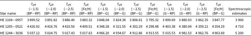
Note. The numbers in the parentheses below $T_{\rm eff}$ indicate the metallicity values at which the temperatures are calculated. The temperatures calculated using the adopted metallicity of the stars are presented in columns 5, 9, and 13. Temperatures are given in Kelvin.

Table 4. Derived atmospheric parameters of our programme stars.

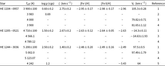
1. Our work, 2. Anders et al. (2022), 3. Gaia Collaboration et al. (2023), 4. Gaia Collaboration et al. (2018), 5. Limberg et al. (2021).

4. Spectroscopic stellar parameters

The radial velocity of the programme stars is calculated by measuring the shift in the observed wavelengths from the lab wavelengths. A good number of clean and unblended lines were selected for this estimation. The values of heliocentric radial velocities are presented in Table 4. The estimated radial velocities are compared with those reported in the published works for the programme stars. The comparison reveals significant variations in the radial velocities of the programme stars except HE 1205 $-$ 0521, suggesting that they may be part of binary systems.

We have derived the stellar atmospheric parameters of the programme stars from the equivalent width measurements of a good number of clean and unblended Fe I and Fe II lines (Table 5). Due to the very metal–poor nature of our programme stars, we were able to identify only a limited number of clean, unblended Fe I and Fe II lines for our analysis. We compiled a linelist for Fe I and Fe II, with the necessary line information sourced from linemake^a (Placco et al. 2021). These lines were then visually identified in the programme stars by overplotting the Arcturus spectrum, as it is a giant star, similar to our programme stars, which are also giants. We made use of MOOG (Sneden 1973, updated version 2019) for the analysis under the assumption of local thermodynamic equilibrium (LTE). We have generated the required model atmospheres using the Kurucz grid of model atmospheres with no convective overshooting http://cfaku5.cfa.hardvard.edu/.

We begin by establishing an initial stellar atmospheric model with estimated values for parameters such as effective temperature ( $T_{\rm eff}$ ), surface gravity (log g), and microturbulent velocity ( $\zeta$ ) as initial guess which are then refined through a series of iterations to derive the final stellar atmospheric parameters. The photometric temperature estimated from the J-K colour index is used as the initial value for $T_{\rm eff}$ because it is independent of metallicity. Given that the metallicity of the programme stars is unknown, this temperature serves as a reliable starting point for determining the final $T_{\rm eff}$ .

Table 5. Equivalent widths (in mÅ) of Fe lines used for deriving atmospheric parameters.

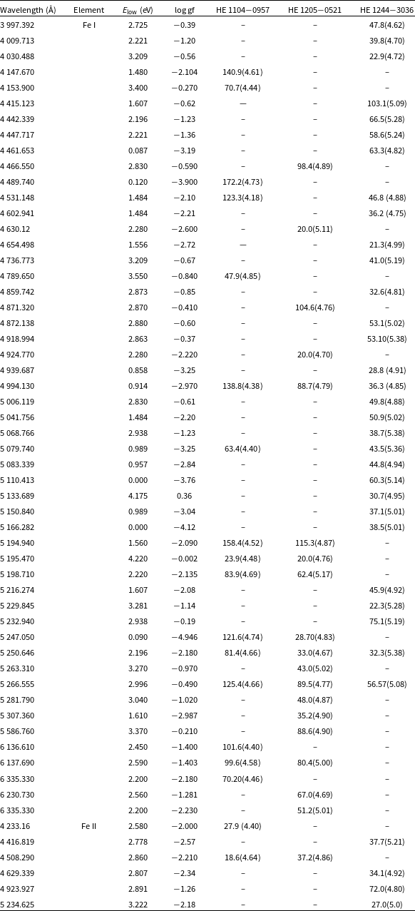
The number in the parenthesis gives the derived abundance ( ${\log}{\epsilon}(X)$ ) from the respective line.

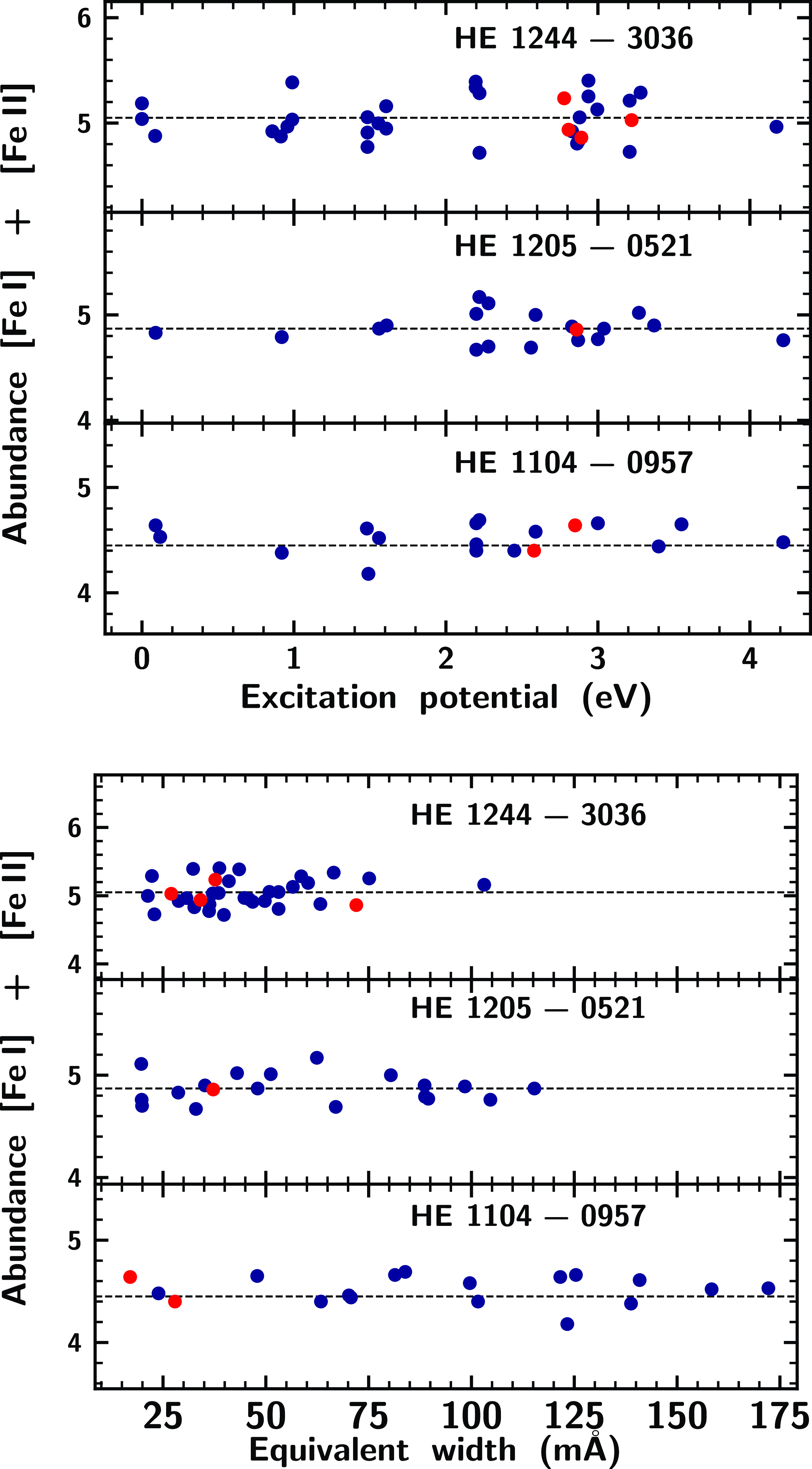
Figure 2. The iron abundances of programme stars as a function of excitation potential (top panel) and equivalent width (bottom panel). In all the panels, the blue-filled circles indicate Fe I lines and the red filled circles represent Fe II lines.

Next, we estimate an initial value for log g. The surface gravity of a star can be derived from its mass and parallax using the equation presented in Yang et al. (2016). To determine the mass, we place the programme stars on the Hertzsprung–Russell (H–R) diagram using evolutionary tracks from Girardi et al. (2000). The star’s luminosity is calculated from its parallax, while the $T_{\rm eff}$ derived from the J–K colour is used as the star’s temperature. Once these parameters are obtained, we can locate the star on the H–R diagram and estimate its mass. The log g is then derived using this mass of the star and the parallax, following the relation provided in Yang et al. (2016). This logg is used as the initial guess for deriving spectroscopic logg using model atmospheres.

Finally, we estimate an initial value for $\zeta$ by substituting the calculated log g into the relation between log g and $\zeta$ as given by Johnson et al. (2007). These initial guesses for log g and $\zeta$ are then used in iterative procedures to determine the final stellar atmospheric parameters, as explained below.

The final values of the stellar atmospheric parameters of the star are determined by a number of iterations in which the initial parameters are changed as follows: The temperature is changed until there exists no trend between the abundances of Fe I and Fe II lines and the corresponding excitation potential. Under this value of effective temperature, microturbulent velocity is changed in such a way that there is no trend between the abundances of Fe I and Fe II lines and the reduced equivalent width (W $_{\lambda}$ / $\lambda$ ), respectively (Fig. 2). Under these values of temperature and microturbulent velocity, log g is changed in a number of iterations in such a way that the abundances derived from Fe I and Fe II lines are nearly the same. The derived atmospheric parameters of the programme stars are presented along with their radial velocities in Table 4.

Although Fe I lines are subject to NLTE effects, we have taken comprehensive measures to ensure that our spectroscopic stellar parameters are reliable and robust. Our analysis is based on a carefully curated selection of Fe I and Fe II lines, avoiding blended or asymmetric features to minimise potential NLTE impacts. The derived parameters satisfy both ionisation equilibrium (Fe I/Fe II) and excitation equilibrium (trends with excitation potential), which are benchmarks of reliable atmospheric estimates. To validate our results, we compared the spectroscopically derived temperatures of our programme stars with photometric estimates using 2MASS and GAIA magnitudes, finding good agreement within error margins. Furthermore, as noted in Ezzeddine, Frebel, & Plez (2017), NLTE effects for Fe I are generally minimal in the metallicity and temperature ranges of our programme stars, further supporting the reliability of our results. These considerations demonstrate that our approach yields robust and trustworthy spectroscopic parameters, consistent with established methods and independent validations.

4.1 Mass and age

We could determine the mass and the age of our programme stars HE 1205 $-$ 0521, and HE 1244 $-$ 3036 from their locations on the H–R diagram (Fig. 3) using the evolutionary tracks and the isochrones from (Girardi et al. 2000) corresponding to $Z=0.0004$ . We could not determine the mass and age for HE 1104 $-$ 0957 as this object falls outside the available tracks and isochrones. The luminosity of the stars is determined using the relation,

\begin{equation*} \log(L/L_{\odot}) = (M_{\odot}-M_{\rm bol})/2.5\end{equation*}

Here M $_{\odot}$ represents the Sun’s bolometric magnitude, and

\begin{equation*} M_{\rm bol} = Mv+BC-Av\end{equation*}

Mv is determined using the equation,

\begin{equation*} Mv = V-(5\log(d))+5\end{equation*}

The visual magnitude V of the stars are adopted from different sources such as Limberg et al. (2021), Høg et al. (2000) and 2MASS survey, and the parallax values are adopted from Gaia (Gaia Collaboration et al. 2023). Bolometric corrections are estimated using the empirical calibrations of Alonso, Arribas, & Martinez–Roger (1999). Interstellar extinctions used for the determination of bolometric magnitude are estimated from the formula given in Schlafly & Finkbeiner (2011). Estimates of the mass and the age from the parallax method are presented in Table 6. We have also determined the log g of the programme stars from this mass, and compared it with the spectroscopic value of log g in Table 6.

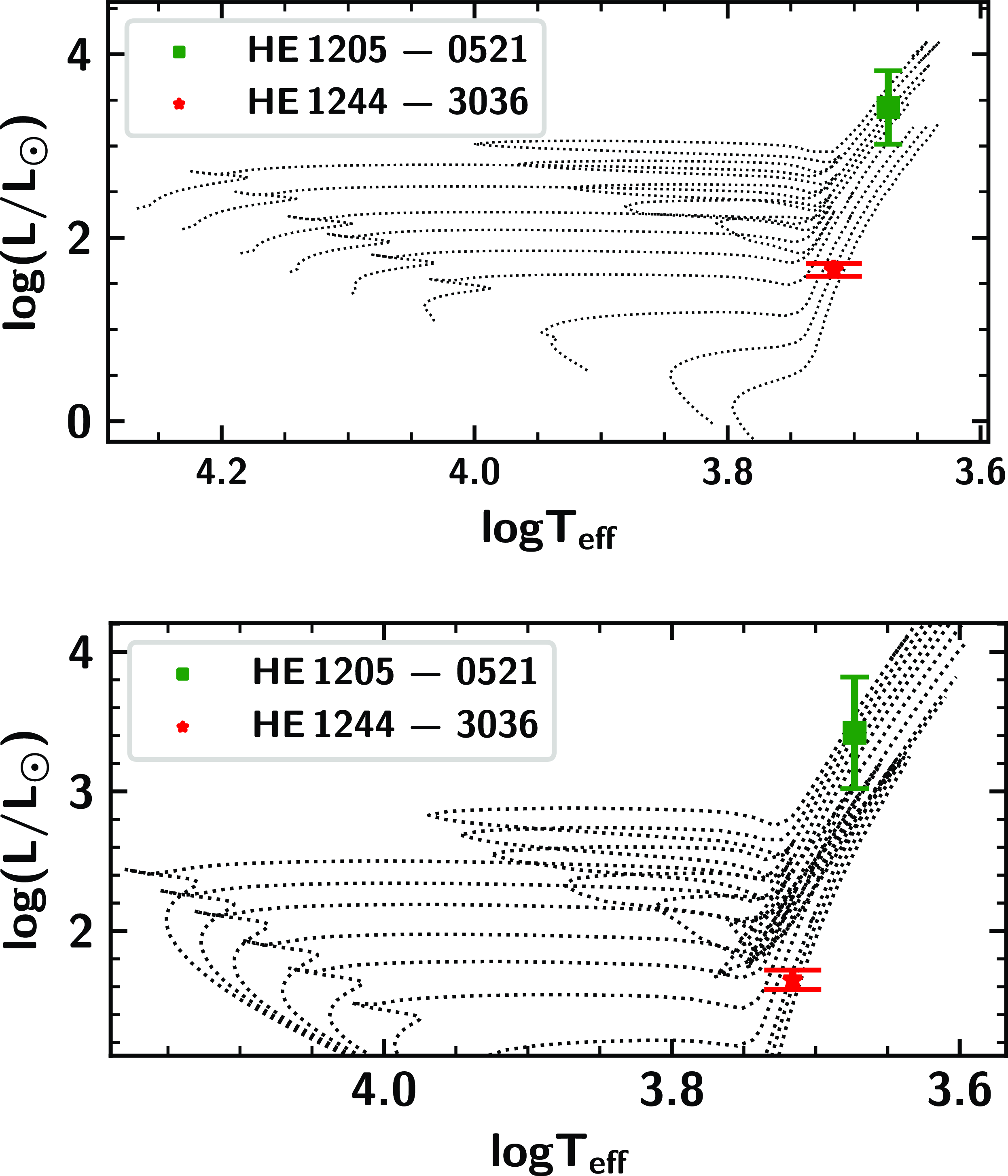
Figure 3. The locations of HE 1205 $-$ 0521, and HE 1244 $-$ 3036 in the H-R diagram are shown. The evolutionary tracks for 0.7, 0.9, 1.2, 1.6, 1.9, 2.2, 2.5, 3, and 3.5 M $_\odot$ are shown from bottom to top in the upper panel. The isochrone tracks for log(age) 10.25, 10.05, 9.85, 9.45, 9.15, 8.95, 8.8, 8.65, 8.54 and 8.45 are shown from bottom to top in the bottom panel.

5. Abundance analysis

We have used equivalent width measurements and spectrum synthesis calculations of clean and unblended lines for the determination of elemental abundances. The lines due to various elements are identified by over–plotting the Arcturus spectrum on the spectra of the programme stars. A master line list is then prepared, including the measured equivalent widths of the lines and other line information such as log gf and excitation potential values. The necessary atomic and molecular line data, including hyperfine structure details, were sourced from the linemake (Placco et al. 2021).

Abundances of the light elements C and N, $\alpha-$ elements such as Mg, Ca, Sc, and Ti, and Fe-peak elements such as Cr, Mn, Co, and Ni are estimated whenever possible. Abundances of neutron-capture elements Sr, Y, Zr, Ba, La, Ce, Pr, Nd, Sm, and Eu are also determined whenever the lines due to these elements could be measured. Spectrum synthesis calculation is performed to determine the abundances of the elements that show hyperfine splitting, such as Sc, V, Mn, Co, Ba, La, and Eu. The details of the abundance analysis are discussed in the following sub-sections, and the abundance results are presented in Table 7. The lines used for the determination of elemental abundances using equivalent width measurements are tabulated and presented as Appendix A.

5.1 Carbon, Nitrogen, and Oxygen

The spectrum synthesis calculation of O forbidden line [OI] 6363.8 Å (Fig. 4) is used to derive the abundance of O. We could derive the O abundance only in HE 1104 $-$ 0957 and HE 1205 $-$ 0521. Since the wavelength range of the spectra of HE 1244 $-$ 3036 does not include the O lines, we could not derive the O abundance in this object. Oxygen is found to be enhanced both in HE 1104 $-$ 0957 and HE 1205 $-$ 0521 with [O/Fe] $\sim$ 1.54 and 1.96, respectively.

Table 6. Estimates of log g using parallax method.

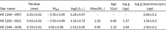
Table 7. Elemental abundances in HE 1104 $-$ 0957, HE 1205 $-$ 0521 and HE 1244 $-$ 3036.

$^{\rm a}$ Asplund et al. (2009), The number inside the parenthesis shows the number of lines used for the abundance determination.

The abundance of C in our programme stars is derived using the spectrum synthesis calculation of the C $_{2}$ band at 5165, and 5635 Å, and the CH band at 4315 Å (Fig. 5). Since the C $_{2}$ band is influenced by O, we have derived the abundance of O first, and then under this O abundance, we derived the C abundance. 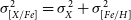In HE 1244 $-$ 3036, we could determine the C abundance only from the CH band as the C $_{2}$ bands are too weak to do the spectrum synthesis calculation. Carbon is enhanced in all three stars with [C/Fe] ranging from 1.06 to 2.15. We could estimate the carbon isotopic ratio only in HE 1205 $-$ 0521, which is found to be $\sim$ 15. Carbon isotopic ratio is determined from the spectrum synthesis calculation of the C $_{2}$ swan system around 4740 Å (Fig. 6)

Nitrogen abundance is determined from the spectrum synthesis of CN band at 3889 Å in HE 1244 $-$ 3036, and 4215 Å in the remaining two stars. CN 3889 Å band is outside the available spectral wavelength coverage for HE 1104 $-$ 0957 and HE 1205 $-$ 0521. The CN band at 4215 Å is saturated in HE 1244 $-$ 3036. Nitrogen is enhanced in all the three stars with [N/Fe] $\gt$ 1.0.

Figure 4. Synthesis of [OI] line around 6363 Å in HE 1104 $-$ 0957. The dotted line represents synthesised spectra, and the solid line indicates the observed spectra. Red short dashed line represents the synthetic spectra corresponding to $\Delta$ [O/Fe] = −0.2 and blue short dashed line corresponds to $\Delta$ [O/Fe] = +0.2

5.2 Mg, Ca, Sc, Ti, and V

Magnesium abundance is derived from the spectrum synthesis of the line Mg I 4571.10 Å in HE 1104 $-$ 0957 and HE 1205 $-$ 0521. We have employed spectrum synthesis calculation for the abundance estimate of Mg as only one good Mg I line is available for these two stars. Other lines found are broad and blended and not usable for equivalent width-based abundance estimations. Abundance of an element derived from the equivalent width measurement of a single line may not be accurate as different lines of the same element can give slightly different abundance values due to various reasons such as the line sensitivity to stellar parameters, blending, non-LTE effects, and line strength. Even if a line appears relatively unblended, small contributions from nearby features can introduce systematic errors into abundance measurements, particularly for weaker lines. Different lines of the same element might be affected differently by blending, causing small shifts in the derived abundance. Similarly, some lines may be more affected by deviations from LTE, particularly for elements like Fe, Na, and Mg. If some lines used in the abundance determination are more prone to non-LTE effects than others, this can introduce systematic differences in the final abundance. To mitigate this, it is advisable to use spectrum synthesis, when only one good line is available, as it accounts for blending and minimises deviations from the mean value. In cases where multiple clean, unblended lines are available, we determine the abundance by averaging results from several lines with different excitation potentials and present it alongside the standard deviation to quantify the error range.

Mg abundance in HE 1244 $-$ 3036 is determined using equivalent width measurements of four Mg I lines (Table A1). The abundance of Mg is determined by spectrum synthesis calculation of the line Mg I 5172.684 Å in HE 1104 $-$ 0957 and HE 1205 $-$ 0521. While it is found to be near solar in HE 1104 $-$ 0957, it is found to be slightly enhanced in HE 1244 $-$ 3036 with [Mg/Fe] $\sim$ 0.60. Calcium abundance is determined from the equivalent width measurements of two Ca I lines for HE 1104 $-$ 0957 and HE 1205 $-$ 0521, and five Ca I lines for HE 1244 $-$ 3036 (Table A1). While Ca abundance in HE 1104 $-$ 0957 is found to be near solar, the Ca abundances in the other two stars are in the range 0.27–0.29 with respect to iron.

In the programme stars, the abundance of Sc is derived using the spectrum synthesis calculation of the lines Sc II 5239.81 Å, considering their hyperfine contributions. While Sc abundance is found to be near solar in HE 1244 $-$ 3036, it is slightly enhanced in HE 1104 $-$ 0957 and HE 1205 $-$ 0521. Titanium abundance is determined from the equivalent width measurements of a number of Ti I and Ti II lines (Table A1). Titanium abundances in our programme stars are in the range 0.32 $\leq$ [Ti/Fe] $\leq$ 0.81. We could derive V abundance from the spectrum synthesis calculation of the line at 6216.354 Å only in HE 1104 $-$ 0957 with a value of $\sim$ 0.72 with respect to Fe. In the remaining two stars, the V I lines are found to be blended and not usable for abundance determination.

5.3 Cr, Mn, Co, and Ni

For the star HE 1104 $-$ 0957, Cr abundance is determined from the equivalent width measurements of two Cr I lines (Table A1). We have used the spectrum synthesis calculation of the line Cr I 5348.31 Å to derive the Cr abundance in HE 1205 $-$ 0521 and HE 1244 $-$ 3036 as this is the only good line of Cr available for these two stars. Chromium is found to be slightly enhanced in HE 1104 $-$ 0957 with [Cr/Fe] $\sim$ 0.76. In the remaining two stars, it is found to be near solar with values $-$ 0.09 and $-$ 0.1 respectively. We have used spectrum synthesis calculation of Mn I 4451.59 for the abundance determination of Mn in HE 1104 $-$ 0957 and HE 1244 $-$ 3036, considering their hyperfine contributions. We could not derive the Mn abundance in HE 1205 $-$ 0521 as no good lines were available. Mn is found to be slightly enhanced in HE 1104 $-$ 0957 with [Mn/Fe] $\sim$ 0.49.

We could determine the abundances of Co and Ni only in HE 1104 $-$ 0957. We have used spectrum synthesis calculation of the lines Co I 4792.85 Å, and Ni I 6128.97 Å for the abundance determination as only one line is available for each of these elements. In the other two stars, we could not find any good lines of Co I and Ni I for abundance determination.

5.4 Sr, Y, and Zr

We could determine the abundance of Sr only in HE 1244 $-$ 3036 as the only available line Sr II 4607.33 Å is found to be very weak and heavily blended in the remaining stars. Strontium is enhanced in HE 1244 $-$ 3036 with [Sr/Fe] $\sim$ 0.95. In HE 1104 $-$ 0957 and HE 1205 $-$ 0521, the abundance of Y is determined from the spectrum synthesis calculation of the lines Y II 4883.68 and 5289.81 Å, respectively. The Y abundance in HE 1244 $-$ 3036 is derived from the equivalent width measurements of two Y II lines (Table A1). It is found to be enhanced in all the three programme stars with [Y/Fe] $\gt$ 0.90.

Zirconium abundance is determined from the spectrum synthesis calculation of the line Zr II 4205.94 Å, in HE 1205 $-$ 0521, and for HE 1244 $-$ 3036 equivalent width measurements of three Zr II lines are used. Zr is found to be enhanced with [Zr/Fe] $\sim$ 1.68 and 1.08, respectively. We could not derive the Zr abundance in HE 1104 $-$ 0957 as the Zr lines are found to be very weak and contaminated.

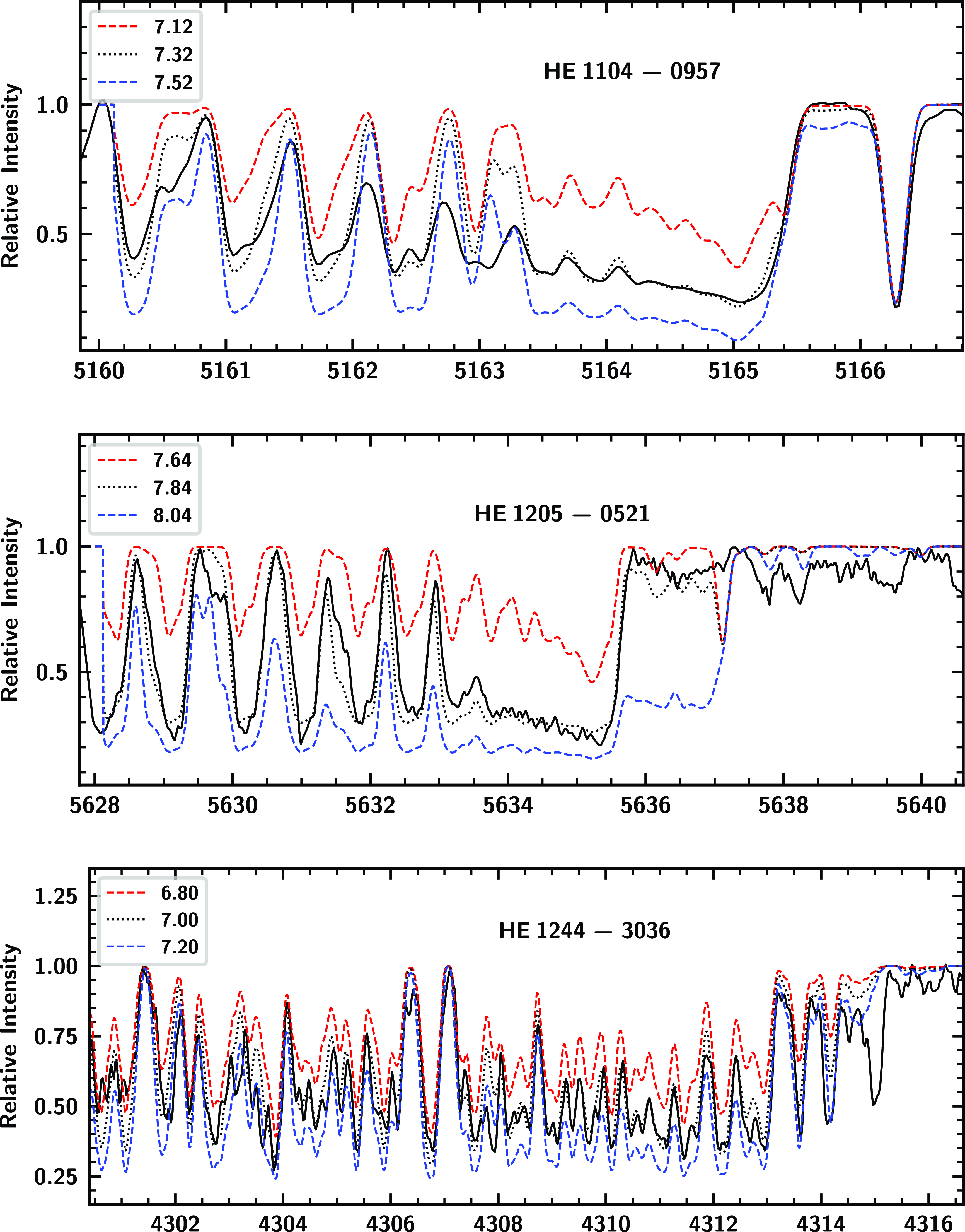
Figure 5. Synthesis of C $_{2}$ band around 5165, 5635 Å, and CH band around 4315 Å. The dotted line represents synthesised spectra, and the solid line indicates the observed spectra. Red short dashed line represents the synthetic spectra corresponding to $\Delta$ [C/Fe] = −0.2 and blue short dashed line corresponds to $\Delta$ [C/Fe] = +0.2

5.5 Ba, La, Ce, Pr, Nd, Sm, and Eu

We have derived the Ba abundance from the spectrum synthesis calculation of Ba II 4934.07 Å in HE 1244 $-$ 3036 (Figure 7). Ba II 5853.67 and 6141.73 Å are used for HE 1104 $-$ 0957 and HE 1205 $-$ 0521, respectively. In HE 1104 $-$ 0957, we could derive only the upper limit to the Ba abundance as the line is broad and blended, and [Ba/Fe] is found to be $\lt$ 0.90 in this star. In HE 1205 $-$ 0521, and HE 1244 $-$ 3036 Ba is found to be enhanced with [Ba/Fe] $\sim$ 1.01, and 2.14 respectively.

Spectrum synthesis calculation of the line La II 4921.78 Å is used to derive the abundance of La in HE 1104 $-$ 0957 and HE 1244 $-$ 3036, and the line La II 6390.48 Å is used in HE 1205 $-$ 0521. While La is enhanced in HE 1205 $-$ 0521 and HE 1244 $-$ 3036 with [La/Fe] $\gt$ 1.0, it is found to be only slightly enhanced in HE 1104 $-$ 0957 with [La/Fe] $\sim$ 0.38.

Spectrum synthesis calculation of Ce II 4562.359 Å is used in HE 1104 $-$ 0957, and Ce II 4483.890 Å in HE 1205 $-$ 0521 to derive the abundance of Ce. We have used the equivalent width measurements of nine Ce II lines to derive the Ce abundance in HE 1244 $-$ 3036. While HE 1205 $-$ 0521 and HE 1244 $-$ 3036 exhibit enhancement of Ce with [Ce/Fe] $\gt$ 1.0, HE 1104 $-$ 0957 exhibits an enhancement with [Ce/Fe] $\sim$ 0.87. We could derive Pr abundance only in HE 1104 $-$ 0957 and HE 1205 $-$ 0521 using the spectrum synthesis calculation of the lines Pr II 4175.62 and 5289.34 Å, respectively. No good lines of Pr II were detected in the spectrum of HE 1244 $-$ 3036. Pr is found to be enhanced in HE 1104 $-$ 0957 and HE 1205 $-$ 0521 with [Pr/Fe] $\sim$ 1.13 and 1.95, respectively.

Neodymium abundance in our programme stars is determined from the equivalent width measurements of a few Nd II lines (Table A1) except for HE 1205 $-$ 0512 for which no good lines of Nd were available for abundance determination. Nd is found to be enhanced in both HE 1104 $-$ 0957 and HE 1244 $-$ 3036. Samarium abundance in our programme stars is determined from the equivalent width measurement of a few Sm II lines (Table A1) except for HE 1205 $-$ 0521 for which we used the spectrum synthesis calculation of the line Sm II 4519.63 Å, the only one good line of Sm II available for HE 1205 $-$ 0521. Sm is found to be enhanced in all of the programme stars. We could derive Europium abundance only in HE 1104 $-$ 0957 and HE 1205 $-$ 0521 from the spectrum synthesis calculation of the lines Eu II 6437.64 and 6645.06 Å respectively. Since the Eu II line is slightly blended and broad, we could derive only an upper limit of Eu abundance ([Eu/Fe] $\lt$ 1.83) for HE 1104 $-$ 0957. The estimated Eu abundance in HE 1205 $-$ 0521 is found to be [Eu/Fe] $\sim$ 1.66. We could not derive Eu abundance in HE 1244 $-$ 3036 as the available Eu lines are found to be very weak and blended and not suitable for abundance estimation. We have included the necessary hyperfine contributions for the abundance estimation of Ba, La, and Eu.

We have determined the elemental abundance ratios such as [ls/Fe], [hs/Fe], and [hs/ls]. [ls/Fe] represents the average of the light s-process elements (Sr, Y, Zr with respect to iron) and [hs/Fe] represents the average of the heavy s-process elements (Ba, La, Ce, Nd with respect to iron). These estimates are presented in Table 8.

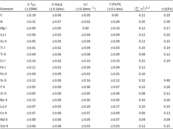
6. Abundance uncertainties

The total error in the derived elemental abundances includes random errors and systematic errors. The uncertainties in the line parameters, such as equivalent widths, line blending, and oscillator strength are the main causes of random errors. Systematic errors are produced by the uncertainties in the stellar atmospheric parameters. Uncertainties in the derived elemental abundances using equivalent width measurement and spectrum synthesis calculation are determined using the procedures as described in Shejeelammal, Goswami, & Shi (2021). The total uncertainties in the estimated elemental abundances, ${log}{\epsilon}(X)$ :

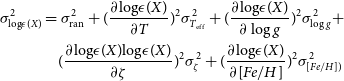(1) \begin{align}\sigma^{2}_{{\log}{\epsilon}(X)} &= \sigma^{2}_{\rm ran}+(\frac{\partial {\log}{\epsilon}(X)}{\partial T})^{2} \sigma_{T_{\rm eff}}^{2}+(\frac{\partial {\log}{\epsilon}(X)}{\partial \log g})^{2}\sigma^{2}_{\log g}+\nonumber\\&\quad(\frac{\partial {\log}{\epsilon}(X){\log}{\epsilon}(X)}{\partial \zeta})^{2}\sigma^{2}_{\zeta}+(\frac{\partial {\log}{\epsilon}(X)}{\partial [Fe/H]})^{2}\sigma^{2}_{[Fe/H])}\end{align}

where $\sigma^{2}_{\rm ran}$ = $\sigma_{s}/\sqrt{N}$ . $\sigma_{s}$ represents the standard deviation in the abundance of an element derived using N number of lines due to that element. The $\sigma$ ’s represent the uncertainties in the adopted stellar atmospheric parameters and are as follows: $T_{\rm eff}$ $\sim$ $\pm$ 100 K, log g $\sim$ $\pm$ 0.2 dex, $\zeta$ $\sim$ $\pm$ 0.2 km s $^{-1}$ , and [Fe/H] $\sim$ $\pm$ 0.1 dex. The uncertainty in [X/Fe] is determined using the relation :

(2) \begin{align}\sigma^{2}_{[X/Fe]} = \sigma^{2}_{X} + \sigma^{2}_{[Fe/H]} \end{align}

The differential elemental abundances (as given by equation (2)) for the object HE 1244 $-$ 3036 are given in Table 9. The error in the elemental abundances derived using the spectrum synthesis calculation is taken as 0.2 dex (indicated by ‘syn’ in Tables 7), which represents the minimum change in the abundance value required to produce well–distinguished synthetic spectra with respect to the best fits. The errors corresponding to the elemental abundances derived using the equivalent width measurements represent the standard deviation (Table 7).

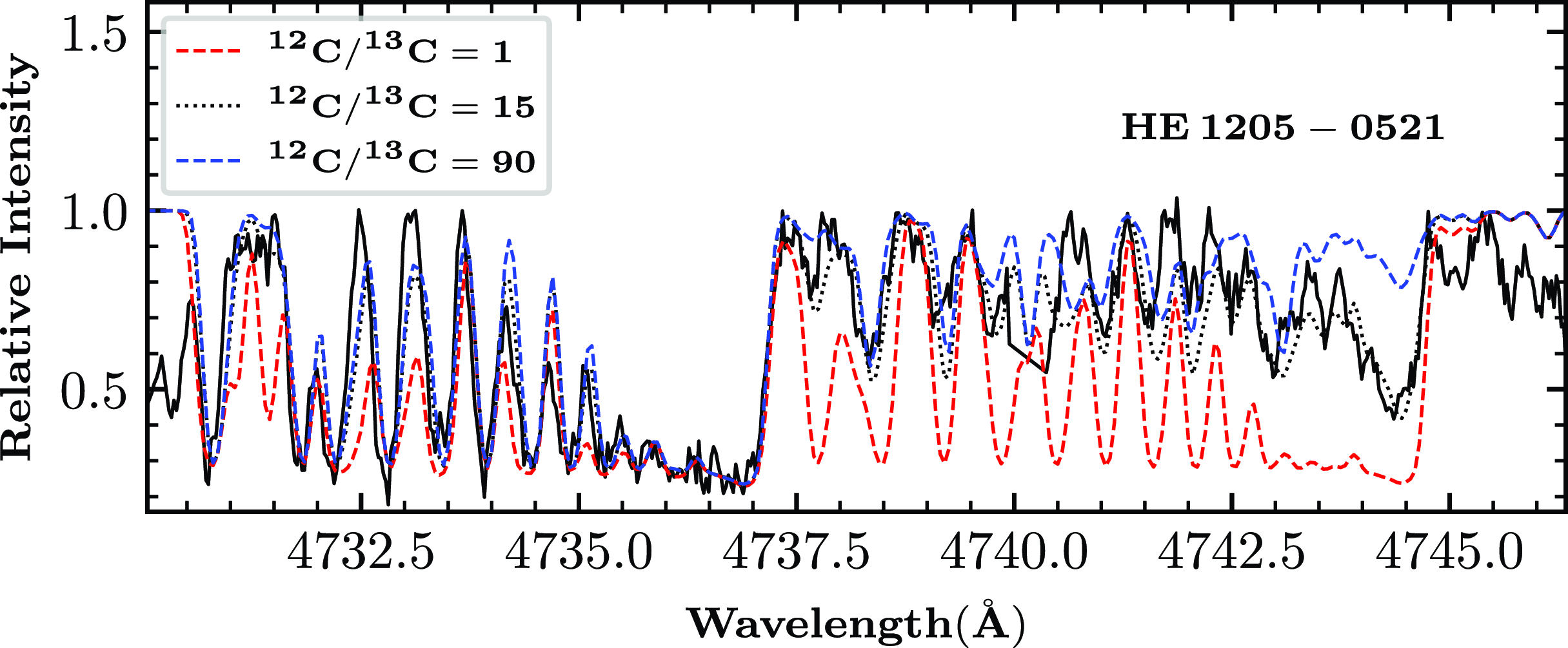
Figure 6. Spectral synthesis fits of the C $_{2}$ features around 4740 Å in HE 1205 $-$ 0521. The solid line indicates the observed spectra. Short and long dashed lines are shown to illustrate the sensitivity of the line strengths to the isotopic carbon abundance ratios

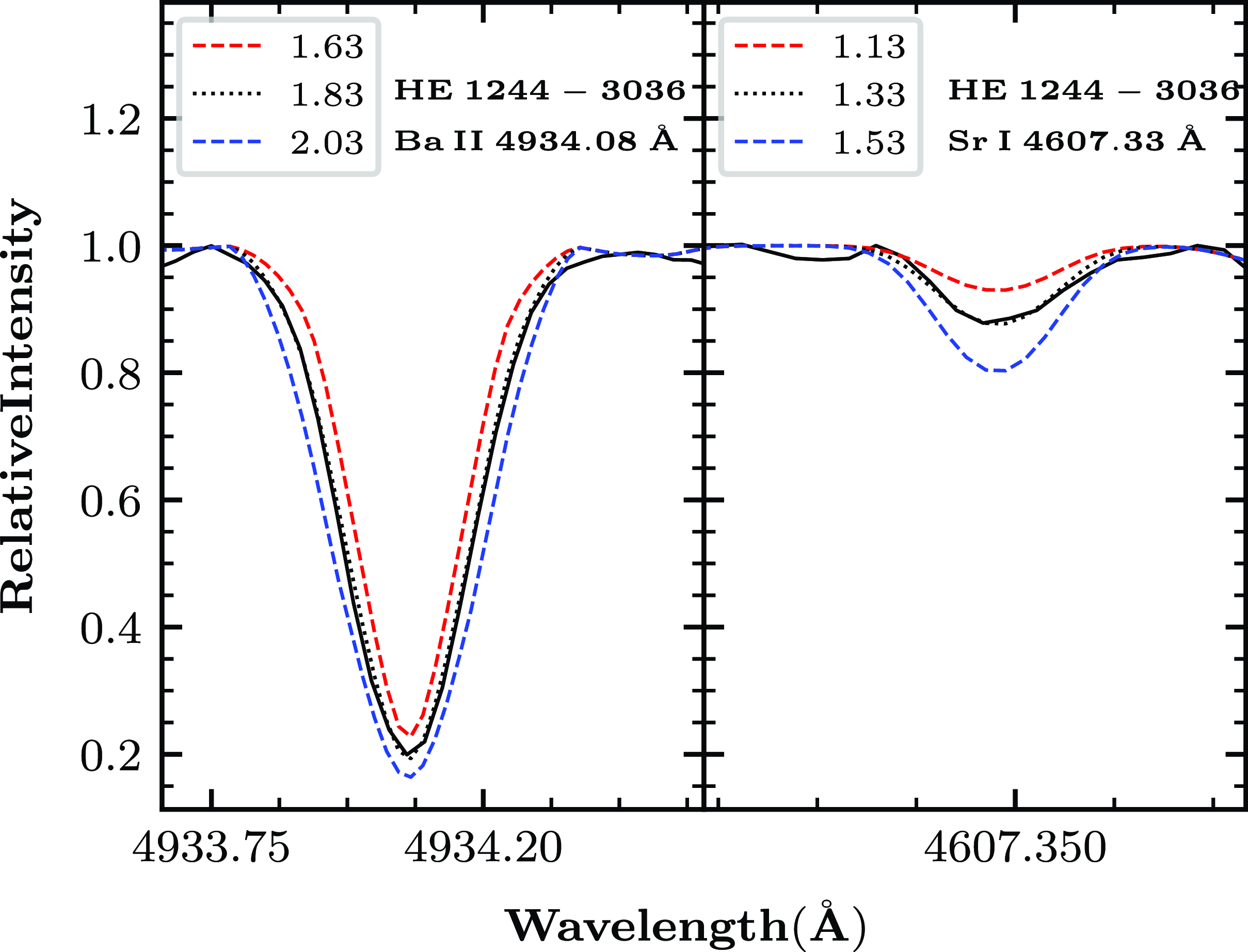
Figure 7. Synthesis of Ba II around 4934.08 Å, and Sr II around 4607.33 Å in HE 1244 $-$ 3036. The dotted line represents synthesised spectra, and the solid line indicates the observed spectra. Red short dashed line represents the synthetic spectra corresponding to $\Delta$ [X/Fe] = −0.2 and blue short dashed line corresponds to $\Delta$ [X/Fe] = +0.2.

Table 8. Estimates of [Fe/H], [ls/Fe], [hs/Fe], [hs/ls] and $^{12}$ C/ $^{13}$ C.

Table 9. Differential elemental abundances ( ${\log}{\epsilon}(X)$ ) derived for the object HE 1244 $-$ 3036.

7. Discussions

We have performed a detailed high–resolution spectroscopic analysis for three faint high latitude carbon stars HE 1104 $-$ 0957, HE 1205 $-$ 0521, and HE 1244 $-$ 3036 from the list of Christlieb et al. (2001). Based on a low–resolution (R 1300) spectroscopic analysis Goswami (2005) placed the objects HE 1104 $-$ 0957 and HE 1205 $-$ 0521 in the C–R stars category. However, our analysis based on high–resolution spectra shows that these two objects do not show the characteristic properties of typical C–R stars. On the contrary to C–R stars that normally show near solar abundances of heavy elements, these objects are found to show enhancement of heavy elements. Although carbon and neutron–capture elements in these objects are found to be enhanced and somewhat similar to the majority of CEMP stars, we could not place these two objects in any of the sub–classes of the CEMP stars, based on various elemental abundance ratios and using the classification criteria of CEMP stars (Beers & Christlieb 2005), and (Goswami, Rathour, & Goswami 2021a).

Based on our kinematic analysis (details provided in Section 8), we identify both programme stars as belonging to the Galactic halo. However, their chemical compositions differ significantly from those of typical halo stars. Interestingly, we find a strong match between the abundance patterns of our programme stars and those of stars in the Reticulum II galaxy (Figs. 8 and 9). This suggests that HE 1104 $-$ 0957 and HE 1205 $-$ 0521 may have originated in the Reticulum II galaxy and were subsequently accreted into the Milky Way during past accretion events. While this chemical match is compelling, it does not provide definitive evidence of origin, as other ultra-faint dwarf galaxies (UFDs) with similar enrichment histories could exhibit comparable abundance patterns. Furthermore, the proper motions of our programme stars do not align with those of Reticulum II stars. However, given the limited proper motion data available for Reticulum II stars, these constraints prevent us from drawing robust conclusions about a direct association. Towards this line, we have conducted a detailed chemodynamical analysis for our programme stars, and presented in Section 9 in greater detail.

As we could not estimate Eu abundance for the object HE 1244 $-$ 3036, the CEMP stars classification criteria involving Eu abundance could not be used to classify this object. However, the object is found to be a likely CEMP-s star, as the observed abundance pattern in HE 1244 $-$ 3036 is found to match well when compared with the yields of a 2 M $_{ \odot}$ AGB star with [Fe/H] = $-$ 2.50 as discussed in the following sections. The details of the possible progenitors of our programme stars, and the signatures of internal mixing are also discussed in the following sub-sections.

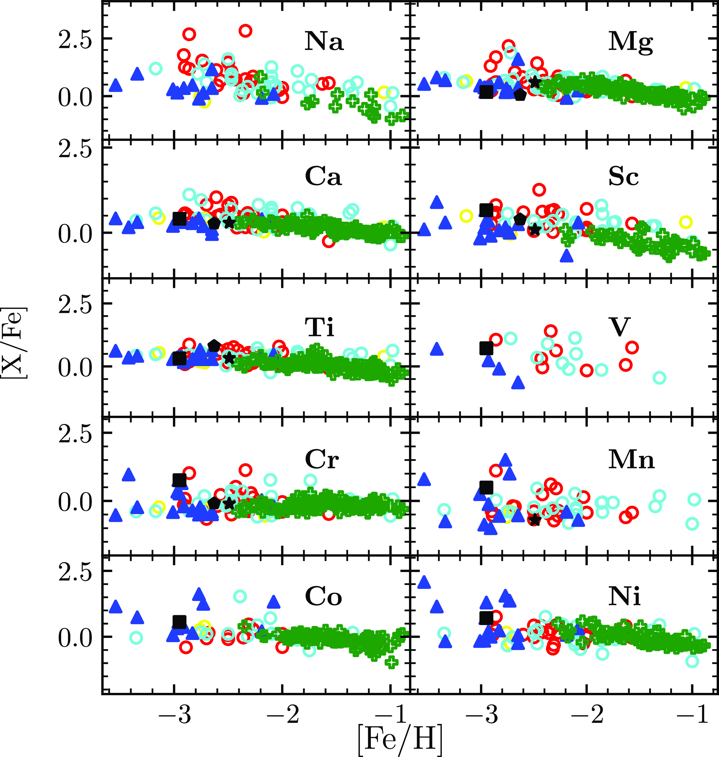
Figure 8. A comparison of the light elements abundance ratios with their counterparts observed in Galactic stars, Sculptor dwarf galaxy stars, and Reticulum galaxy stars. Comparisons are shown for elements for which data from prior works are available. Sculptor dwarf galaxy stars from Skúladóttir et al. (2017), Hill et al. (2019). The abundance values for CEMP–no stars used for the comparison are taken from Christlieb et al. (2004), Plez & Cohen (2005), Yong et al. (2013), Hansen et al. (2014), Bonifacio et al. (2015), Bessell et al. (2015) and Frebel (2018). The abundance values for CEMP–s and CEMP–r/s stars are taken from Lucatello et al. (2003), Barklem et al. (2005), Cohen et al. (2006), Goswami et al. (2006), Aoki et al. (2007), Karinkuzhi & Goswami (2015), Purandardas et al. (2019b,a), Shejeelammal, Goswami, & Shi (2021), Purandardas & Goswami (2021) and Goswami, Rathour, & Goswami (2021a). The symbols used are as follows: red circle = CEMP–rs, cyan circles = CEMP–s, yellow circles = CEMP–no, blue triangles = reticulum, black square = HE 1104–0957, black pentagon = HE 1205–0521, black star = HE1244–3036, green plus = sculptor dwarf galaxy.

Figure 9. Same as Fig. 8, but for heavy elements.

7.1 Locations of the programme stars in the A(C) vs. [Fe/H] diagram:

CEMP stars are found to exhibit bimodal distribution in the absolute carbon (A(C)) vs. metallicity ([Fe/H]) diagram (Spite et al. 2013; Bonifacio et al. 2015; Hansen et al. 2015; Yoon et al. 2016). In this diagram, Yoon et al. (2016) suggested a higher carbon band which peaks around A(C) $\sim$ 7.96 and a lower band peaking at A(C) $\sim$ 6.28. Yoon et al. (2016) classified the objects falling on this diagram into three groups: Group I, Group II, and Group III. The first group exhibits very weak dependence of A(C) on [Fe/H] and are mostly composed of CEMP–s and CEMP–r/s stars. A large fraction of them are confirmed binaries. The remaining two groups are composed of extremely metal–poor objects, including a significant proportion of CEMP–no stars. These two groups are found to be clustered around the lower carbon band. While Group II objects exhibit a clear dependence of A(C) on [Fe/H], Group III objects do not show any dependence of A(C) on [Fe/H]. Both these groups are found to be single stars without any evidence of binary companions.

We have examined the location of the programme stars in the A(C) vs. [Fe/H] diagram (Fig. 10). In order to locate our programme stars in the A(C) vs. [Fe/H] diagram, we applied a correction in the estimated carbon abundance using the public online tool by (Placco et al. 2014).^b The corrections applied to the estimated carbon abundance are 0.32 for HE 1104 $-$ 0957, 0.12 for HE 1205 $-$ 0521, and 0.02 for HE 1244 $-$ 3036, respectively. As a result, the corrected carbon values ( ${\log}{\epsilon}(c)$ $_{\rm corrected}$ ) are 7.64 for HE 1104 $-$ 0957, 8.07 for HE 1205 $-$ 0521, and 7.02 for HE 1244 $-$ 3036. From the location of our programme stars in the A(C) vs. [Fe/H] diagram, we found that HE 1104 $-$ 0957 and HE 1205 $-$ 0521 are Group I objects, and HE 1244 $-$ 3036 fall in the region where Group I and Group II objects overlap. Although many of the Group II objects are single stars, most of the Group I objects are known to be in binary systems.

We have also observed radial velocity variations in the programme stars by comparing our estimates with previously published radial velocities (Table 4). This suggests that the programme stars HE 1104 $-$ 0957 and HE 1244 $-$ 3036 are likely binaries. The enhancement of carbon and other heavy elements may therefore be attributed to binary mass transfer; this possibility is further examined and discussed in the following sub-sections.

Figure 10. Corrected A(C) vs. [Fe/H] diagram for the compilation of CEMP stars taken from Yoon et al. (2016). Cyan symbols indicate CEMP–r/s stars: binary stars are represented by circles, and stars with no information about the binary status are indicated by ‘star’ symbols. CEMP–s stars are represented using green symbols: open and filled circles indicate binary and single stars, respectively. Stars with no information about the binarity are represented using open triangles. Red symbols represent Group II CEMP–no stars: open and filled hexagons represent binary and single stars, respectively. Stars with no information about the binarity are presented using open squares. Group III CEMP–no stars are represented using red symbols: binary and single stars are represented by open and filled pentagons, respectively. Inverted triangles represent stars with no information about the binary status. The short dashed line represents [C/Fe] = 0.7.

7.2 Possible progenitors of the programme stars

The oxygen abundance and the [Sr/Ba] ratio are important indicators of the possible progenitors of a star (Choplin et al. 2017). Based on the analysis of four non–binary CEMP–s stars, Choplin et al. (2017) found that the observed surface chemical composition of three of them can be well explained using the models of fast–rotating massive stars (hereafter FRMS). Their analysis shows that the oxygen abundance of a star whose possible progenitor is an FRMS falls in the range between 1.5 and 2. Many studies have shown that most of the CEMP–s stars are in binary systems and their observed surface chemical composition is attributed to the binary companion (McClure & Woodsworth 1990; Preston & Sneden 2001; Hansen et al. 2016b; Jorissen et al. 2016). In this kind of CEMP stars that are in binary systems, the oxygen abundance falls in the range $-0.2$ $\lt$ [O/Fe] $\lt$ 1.2 (Karakas 2010). Thus, the oxygen abundance works as an useful indicator of the progenitor of a star. We could determine the abundance of oxygen only in HE 1104 $-$ 0957 and HE 1205 $-$ 0521. In both the stars, [O/Fe] $\gt$ 1.5, which indicates an FRMS as a possible progenitor for these objects. This also underscores the implausibility of AGB stars as the progenitors of these stars. This is verified by comparing the surface chemical compositions of these stars with that of the AGB stars at different metallicities and masses using FRANEC Repository of Updated Isotopic Tables & Yields (FRUITY) models (Cristallo et al. 2009, 2011, 2015) following the detailed procedure as discussed in Shejeelammal, Goswami, & Shi (2021) (the data are publicly available at http://fruity.oa-teramo.inaf.it/). We could not reproduce all of the observed elemental patterns of these stars with any of the available models. As we could not derive the abundance of Sr, we could not verify the above results based on the [Sr/Ba] ratio, which could also be used as an indicator if the progenitor of a star is an AGB companion or an FRMS. Studies by Frischknecht, Hirschi, & Thielemann (2012) showed that [Sr/Ba] $\gt$ 0 for massive rotating stars and [Sr/Ba] $\lt$ 0 for AGB stars, and this result is further supported by Choplin et al. (2017).

The [ls/hs] ratio is another important indicator of the progenitor of a star. While the AGB models predict [ls/hs] $\lt$ 0 (Abate et al. 2015), the models of FRMS predict [ls/hs] $\geq$ 0 (Choplin et al. 2017; Chiappini 2013; Cescutti et al. 2013). We could estimate the abundance of only Y in HE 1104 $-$ 0957 among the light s–process elements, and hence, it is not possible to find the [ls/Fe] ratio in this star to draw a robust conclusion. The estimated [ls/hs] ratio for HE 1205 $-$ 0521 is 0.36 which further confirms FRMS as the possible progenitor for this object.

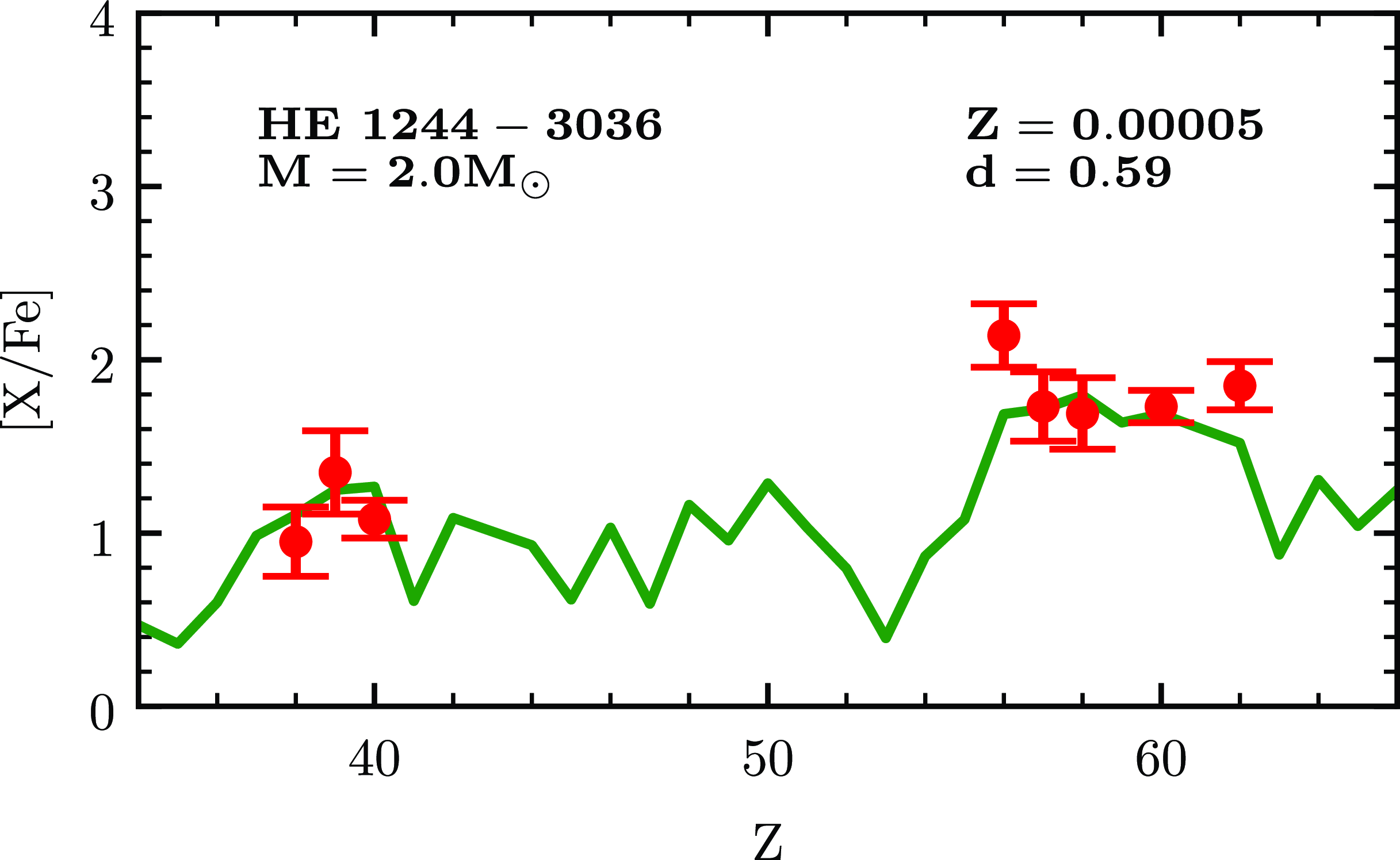
Figure 11. Best-fitting FRUITY model (solid green curve) for HE 1244 $-$ 3036. The points with error bars indicate the observed abundances.

The [O/Fe], as well as the [Sr/Fe] ratios in HE 1244 $-$ 3036, fall in the range expected for an AGB star. We have further confirmed this result by comparing the abundance patterns of HE 1244 $-$ 3036 with the model predictions of AGB stars provided by FRUITY models. For this star, the best fit is obtained for the model with metallicity, z = 0.00005, and mass, M = 2 M $_{\odot}$ (Fig. 11). This further confirms the binary nature of this star. The estimated value of [ls/hs] ratio (= $\,-0.59$ ) in this object again supports the binary mass transfer as the possible source of the observed surface chemical composition of this star.

Elemental abundance ratios like [Mg/C], [Sc/Mn], [C/Cr] and [Ca/Fe] can give insight into the pollution events that have made significant contributions to the surface chemical composition of the star. Based on the cosmological models, Hartwig et al. (2018) presented a number of diagnostic elements to identify stars formed from the gas polluted by the previous supernova. Their analysis results show that [Mg/C] $\lt$ $-1.0$ , [Sc/Mn] $\lt$ 0.50, [C/Cr] $\gt$ 0.50 and [Ca/Fe] $\gt$ 2 indicate mono–enrichment of a star. These ratios estimated for HE 1104 $-$ 0957 and HE 1205 $-$ 0521 indicate that they are mono–enriched. Various diagnostic elemental abundance ratios estimated in HE 1244 $-$ 3036 show that its surface composition is both mono– and multi–enriched, which does not fit with the results from Hartwig et al. (2018). This indicates that the different diagnostic elements in this star do not originate from the previous supernova, and it may be attributed to their binary companion.

7.3 Mixing diagnostic

As all of the programme stars are found to be luminous objects, the observed chemical compositions of the stars might have been altered by any extra–mixing processes (Gratton et al. 2000; Spite et al. 2005). Hence, we have examined whether the surface chemical compositions of the stars are modified by any mixing process using [C/N] and $^{12}C$ / $^{13}$ C ratios (Figs. 12, and 13). Based on [C/N] ratio, HE 1104 $-$ 0957 and HE 1244 $-$ 3036 are found to be well mixed. However, HE 1205 $-$ 0521 does not show any signature of mixing. Although [C/N] ratio can be used as an indicator of mixing, Spite et al. (2006) suggested that [C/N] ratio is not a reliable indicator of mixing due to significant variations in carbon and nitrogen abundances within the interstellar medium. In this context, $^{12}$ C/ $^{13}$ C can be used as a reliable indicator of mixing as it is high in primordial matter and is not sensitive to the choice of stellar atmospheric parameters. While $^{12}$ C/ $^{13}$ C $\lt$ 10 indicates internal mixing in the stars, any value of $^{12}$ C/ $^{13}$ C $\gt$ 10 shows that the star has not undergone any kind of internal mixing (Spite et al. 2006). However, we could not determine $^{12}$ C/ $^{13}$ C ratio in any of our programme stars except HE 1205 $-$ 0521. This star with $^{12}$ C/ $^{13}$ C $\sim$ 15 shows no signature of mixing based on the carbon isotopic ratio.

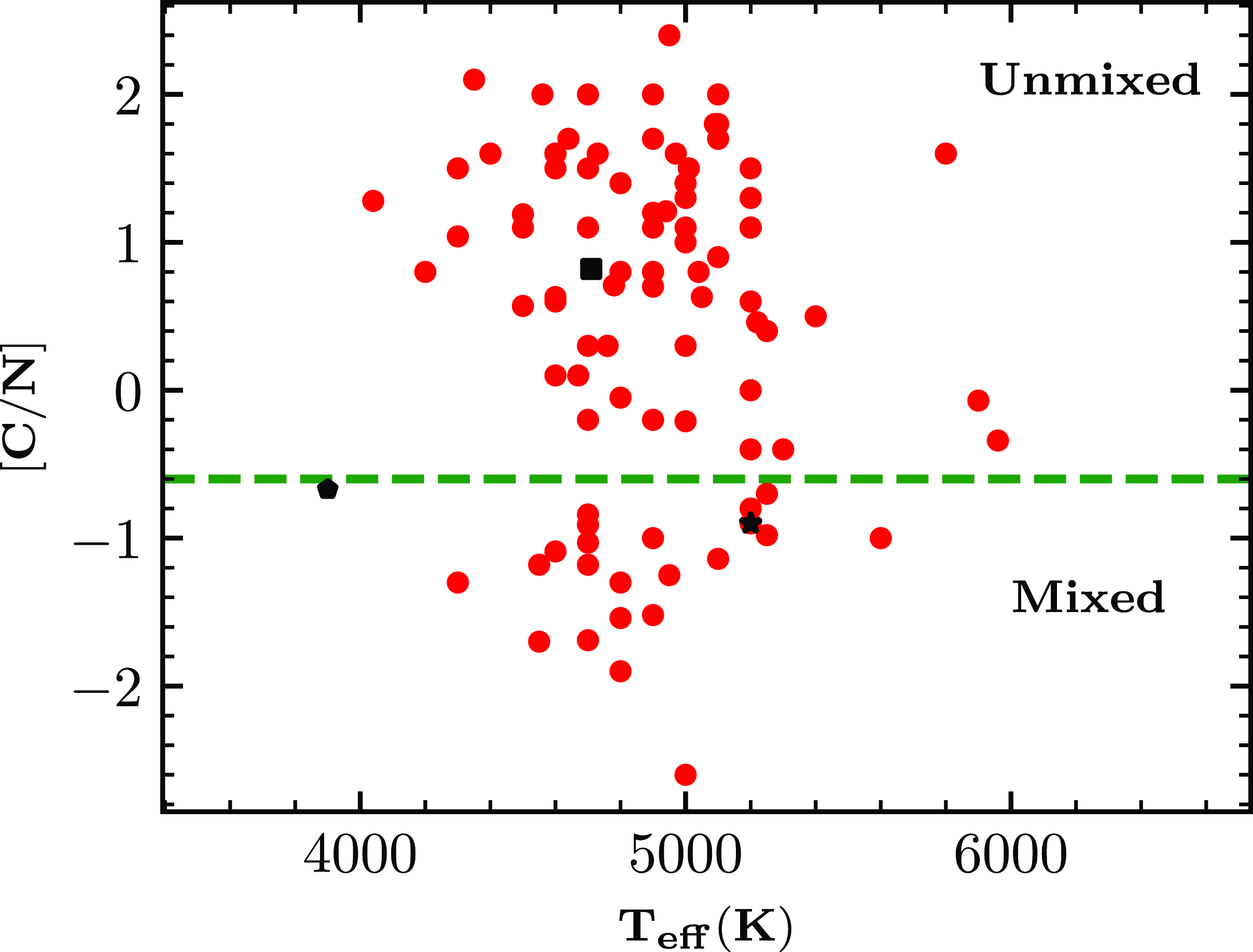
Figure 12. Positions of the programme stars in the [C/N] vs. $T_{\rm eff}$ diagram. Symbols used for the programme stars are the same as in previous Figures. Filled circles represent the stars from prior works (Spite et al. 2006; Aoki et al. 2007; Goswami, Aoki, & Karinkuzhi 2016; Hansen et al. 2016a; Hansen et al. 2019; Purandardas et al. 2019a,b; Goswami, Rathour, & Goswami 2021a; Shejeelammal, Goswami, & Shi 2021).

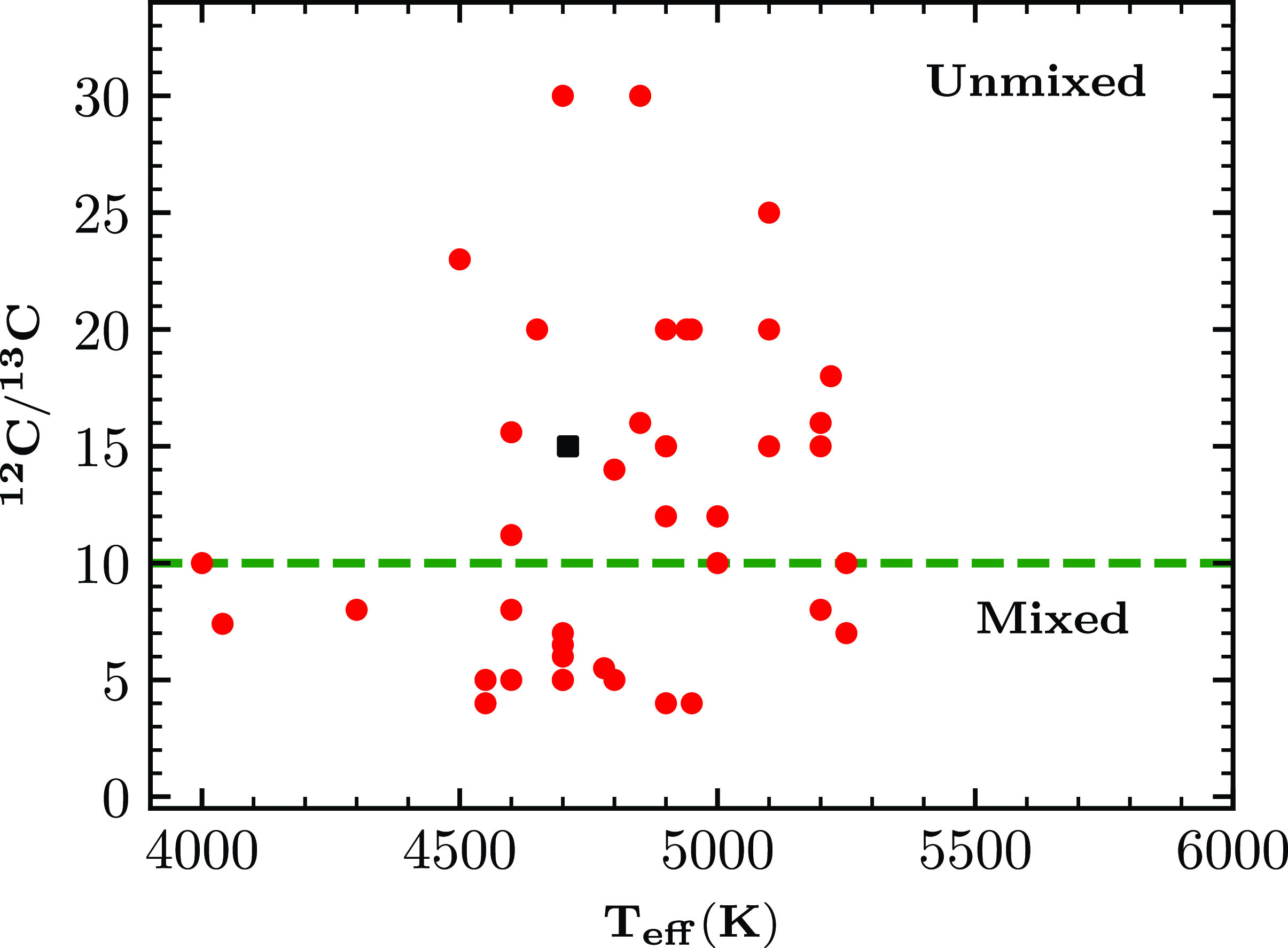
Figure 13. The location of HE 1205 $-$ 0521 (filled square) in the $^{12}$ C/ $^{13}$ C vs. $T_{\rm eff}$ diagram. The filled circles represent the stars from Spite et al. (2006) and Aoki et al. (2007).

Table 10. Spatial velocity and probability estimates for the programme stars.

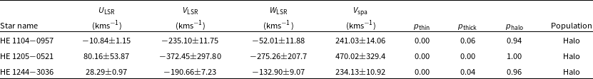
8. Kinematic analysis

Space velocities of the programme stars are estimated using the procedure as described in Bensby, Feltzing, & Lundström (2003). The space velocity with respect to the Local Standard of Rest (LSR) is expressed as:

\begin{align*}(U, V, W)_{LSR} =(U,V,W)+(U, V, W)_{\odot}\ \text{km}\ \text{s}^{-1}\end{align*}

where, $(U, V, W)_{\odot} =(11.1, 12.2, 7.3)$ km s $^{-1}$ (Schönrich, Binney, & Dehnen 2010), and

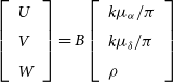\begin{align*}\left[\begin{array}{lll} & U & \\ & V & \\ & W &\end{array} \right] = B\left[\begin{array}{lll} & k\mu_{\alpha }/\pi & \\ & k\mu_{\delta }/\pi & \\& \rho &\end{array} \right]\end{align*}

where B = T.A, $k = 4.74057$ km s $^{-1}$ , $\mu _{\alpha }$ represents the proper motion in right ascension, in arcsec yr $^{-1}$ , $\mu _{\delta }$ is the proper motion in declination, in arcsec yr $^{-1}$ , $\rho$ represents the radial velocity in km s $^{-1}$ and $\pi$ is the parallax in arcsec.

The transformation matrix is given by:

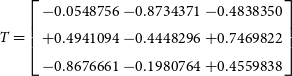\begin{align*}T = \left[\begin{array}{ccc}-0.0548756 & -0.8734371 & -0.4838350 \\+0.4941094 & -0.4448296 & +0.7469822 \\-0.8676661 & -0.1980764 & +0.4559838\end{array} \right]\end{align*}

Coordinate matrix A can be represented as:

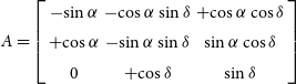\begin{align*}A = \left[\begin{array}{ccc}-\!\sin\alpha & -\!\cos\alpha \sin\delta & +\!\cos\alpha \cos\delta \\+\!\cos\alpha & -\!\sin\alpha \sin\delta & \sin\alpha \cos\delta \\0 & +\!\cos\delta & \sin\delta\end{array} \right]\end{align*}

Where $\alpha$ represents the right ascension and $\delta$ is the declination in degrees. Space velocities of the programme stars are estimated based on a right–handed coordinate system in which the three components of the space velocities are directed in such a way that, U is positive in the direction of Galactic centre, V is positive in the direction of Galactic rotation, and W is positive in the direction of the North Galactic Pole (Johnson & Soderblom 1987). The proper motion and parallax values required for the calculations of space velocities are taken from 2MASS survey (Cutri et al. 2003) and Gaia (Gaia Collaboration et al. 2023), respectively. The radial velocity of the star used in this calculation is our radial velocity estimate.

The total spatial velocity of a star is given by

$V_{spa}^{2}=U_{LSR}^{2}+V_{LSR}^{2}+W_{LSR}^{2}$

We have calculated the probability of our programme star’s membership in our galaxy following the procedures of Reddy, Lambert, & Allende Prieto (2006), Bensby, Feltzing, & Lundström (2003, 2004), and Mishenina et al. (2004). It is based on the assumption that the Galactic space velocities of these stars have Gaussian distributions.

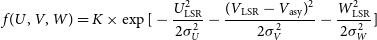\begin{align*}f(U,V,W) = K\times\exp[-\frac{U_{\rm LSR}^{2}}{2\sigma _{U}^{2}}-\frac{(V_{\rm LSR}-V_{\rm asy})^{2}}{2\sigma _{V}^{2}}-\frac{W_{\rm LSR}^{2}}{2\sigma _{W}^{2}}]\end{align*}

where

$K = \frac{1}{(2\pi) ^\frac{3}{2}\sigma _{U}\sigma _{V}\sigma _{W}}$

The values of the characteristic velocity dispersion $\sigma _{U}$ , $\sigma _{V}$ and $\sigma _{W}$ and the asymmetric drift $V_{\rm asy}$ are adopted from Reddy, Lambert, & Allende Prieto (2006). Our estimates show that all of these stars belong to the Halo population with a probability of $\gt$ 94%. The spatial velocities and the probability estimates for the programme stars are presented in Table 10. For HE 1205 $-$ 0521, the error in the estimated spatial velocity is significantly large due to the substantial uncertainty in its parallax measurement, which is around 67%. This level of uncertainty could similarly affect its galactic membership classification.

9. Orbital properties and potential associations of the programme stars with the Galactic Substructures

We have derived the orbital properties of our programme stars using the galpy (http://github.com/jobovy/galpy, Bovy et al. (2012)) python package for Galactic dynamics. We have used astrometric data such as $\alpha$ , $\delta$ , $\mu_{\alpha}$ , $\mu_{\delta}$ , and distance required for the calculations from Gaia DR3 (Gaia Collaboration et al. 2022). Additionally, we used our radial velocity estimates for the programme stars in the analysis. The Galactocentric distance of the sun is taken to be ro = 8 kpc, and the velocity at this distance is taken as 220 kms $^{-1}$ (Bovy et al. 2012). The vertical distance of the sun above the plane is set at zo = 20.8 pc (Bennett & Bovy 2019). The adopted solar motion with respect to the local standard of rest is (U, V, W) = (11.1, 12.2, 7.3) km s $^{-1}$ (Schönrich, Binney, & Dehnen 2010). The detailed procedure can be found in Shejeelammal & Goswami (2024).

We found that both HE 1104 $-$ 0957 and HE 1244 $-$ 3036 are bound to the galaxy based on the value of their energy (Table 11). Whereas HE 1205 $-$ 0521 has slightly higher energy than the rest of the stars, and it is found to be $E_{\rm tot}$ $\sim$ 0.13 km $^{2}\textit{s}^{-2}$ .

From the estimated values of $L_{z}$ and $V_{\phi}$ , we find that both HE 1104 $-$ 0957 and HE 1244 $-$ 3036 are in prograde motion ( $L_{z}$ , $V_{\phi}$ $\gt$ 0), and HE 1205 $-$ 0521 is in retrograde motion ( $L_{z}$ , $V_{\phi}$ $\lt$ 0). The estimated apocentric distances ( $r_{\rm apo}$ ) for HE 1104 $-$ 0957 and HE 1244 $-$ 3036 are 9.23 and 8.02 kpc, respectively, and hence they are probably in the inner–halo (6 $\leq r_{\rm apo}$ $\leq$ 13 kpc for the inner halo, Roederer et al. 2018). For HE 1205 $-$ 0521, the estimated $r_{\rm apo}$ $\sim$ 108.93 kpc, and it belongs to the outer halo ( $r_{\rm apo}$ $\sim$ 15–20kpc corresponds to the outer halo Carollo et al. 2007).

Table 11. Orbital parameters for the programme stars.

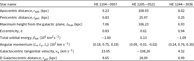
From our detailed chemodynamical analysis of the programme stars, we found that their kinematics deviate from those expected for typical in situ halo stars. Additionally, their chemical properties are inconsistent with those characteristic of in–situ halo stars. To further investigate, we compared their observed orbital properties with those of various Galactic substructures as outlined in Naidu et al. (2020). Although both HE 1104 $-$ 0957 and HE 1244 $-$ 3036 exhibit prograde motion and remain gravitationally bound to the Galaxy, HE 1205 $-$ 0521 displays retrograde motion and a positive total energy, suggesting that it is unbound. This higher, unbound energy poses a constraint for directly comparing the orbital parameters of this star with Galactic substructures based on $E_{\rm tot}$ .

When we compared the orbital parameters of HE 1104 $-$ 0957 and HE 1244 $-$ 3036 with the substructures identified by Naidu et al. (2020), we found a strong resemblance to the Gaia–Sausage–Enceladus (GSE). Although the metallicity distribution function (MDF) of GSE peaks around [Fe/H] $\sim$ –1.15 (Feuillet et al. 2021), it is found that GSE holds stars with metallicities as low as [Fe/H] $\sim$ –2.00 (Naidu et al. 2020). Naidu et al. (2021) provide evidence that GSE is enriched with r–process elements contributed by core–collapse supernovae (CCSNe) and neutron star mergers (NSMs), with CCSNe accounting for approximately 25% of the observed r–process elements. Based on these findings, we propose that the programme stars likely originated in GSE, with their r–process enhancement attributed to the contributions from these enrichment sources, as outlined by Naidu et al. (2021).

Interestingly, observational studies by Ji et al. (2016) have shown that stars in the Reticulum II galaxy exhibit extremely enhanced r-process abundances, consistent with a rare and prolific r-process event such as a neutron star merger. A comparison of the abundance patterns in our programme stars with those of stars in Reticulum II reveals a closer match, raising the possibility of a connection. However, due to uncertainties in the kinematics, we cannot definitively conclude that our programme stars are escapees from Reticulum II. Instead, considering neutron star mergers as a common r-process enrichment source for both GSE and Reticulum II, it is plausible that the programme stars originated in GSE and were enriched by a neutron star merger event (other than the FRMS/AGB progenitor as indicated by the elemental abundance ratios of the programme stars), consistent with the enrichment mechanisms shared by these substructures.

10. Conclusion

Results from the high–resolution spectroscopic analysis of three stars HE 1104 $-$ 0957, HE 1205 $-$ 0521, and HE 1244 $-$ 3036 selected from (Christlieb et al. 2001) are presented. Our analysis shows that the programme stars are very metal–poor and exhibit enhancement of carbon and neutron–capture elements. However, we could not assign any subclass of CEMP stars for HE 1104 $-$ 0957 and HE 1205 $-$ 0521, following the classification criteria for CEMP stars and classification schemes proposed by Beers & Christlieb (2005), and Goswami, Rathour, and Goswami (2021b).

Various elemental abundance ratios estimated in HE 1104 $-$ 0957 and HE 1205 $-$ 0521 show that these objects are mono-enriched with an indication of FRMS as the probable progenitor for these objects. Although, HE 1244 $-$ 3036 could not be classified according to CEMP star classification criteria as the abundance of Eu could not be estimated for this object; the elemental abundance ratios of the object indicate an AGB progenitor for this object based on various diagnostic elemental abundance ratios. The comparison of elemental abundances in this object with that of the AGB yields from FRUITY models further confirms that the AGB star is the progenitor of this object.

The programme stars show signatures of internal mixing based on [C/N] ratio except HE 1205 $-$ 0521. The carbon isotopic ratio is also a useful indicator of mixing. However, we could estimate $^{12}C$ / $^{13}$ C ratio only in HE 1205 $-$ 0521 which does not show any signatures of internal mixing.

We have also estimated the orbital parameters for our programme stars. From the estimated values of $L_{z}$ , and $V_{\phi}$ , we find that both HE 1104 $-$ 0957 and HE 1244 $-$ 3036 are in prograde motion ( $L_{z}$ , $V_{\phi}$ $\gt$ 0), and HE 1205 $-$ 0521 is in retrograde motion ( $L_{z}$ , $V_{\phi}$ $\lt$ 0). Although the estimated apocentric distances for HE 1104 $-$ 0957 and HE 1244 $-$ 3036 indicate that they are probably in the inner halo, the value estimated for HE 1205 $-$ 0521 shows that it belongs to the outer halo.

Although the programme stars are found to be halo objects, the observed abundance patterns do not show a good match with that expected for halo stars. Considering the abundance peculiarities, especially the enhanced r-process elements observed in these stars, we have made a comparison of the abundances of various elements with those of the Reticulum II stars. The abundance patterns strongly match those of stars in the Reticulum II galaxy, suggesting a possible origin in Reticulum II followed by accretion into the Milky Way. However, while this chemical similarity is compelling, the current proper motion data for Reticulum II stars are insufficient to confirm a direct association, as discussed in our detailed chemodynamical analysis (Section 9).

The orbital parameters of HE 1104 $-$ 0957 and HE 1244 $-$ 3036 strongly resemble those of the GSE, which hosts stars with metallicities as low as [Fe/H] $\sim$ $-$ 2.00 and r-process enrichment from CCSNe and NSMs. While the abundance patterns of our programme stars closely match those of Reticulum II, suggesting a possible link, kinematic uncertainties prevent a definitive conclusion. Instead, their r-process enrichment likely originated in GSE, consistent with neutron star merger events shared by both GSE and Reticulum II.