Existential Notation3 Logic

Abstract

In this paper, we delve into Notation3 Logic (N3), an extension of Resource Description Framework (RDF), which empowers users to craft rules introducing fresh blank nodes to RDF graphs. This capability is pivotal in various applications such as ontology mapping, given the ubiquitous presence of blank nodes directly or in auxiliary constructs across the Web. However, the availability of fast N3 reasoners fully supporting blank node introduction remains limited. Conversely, engines like VLog or Nemo, though not explicitly designed for Semantic Web rule formats, cater to analogous constructs, namely existential rules.

We investigate the correlation between N3 rules featuring blank nodes in their heads and existential rules. We pinpoint a subset of N3 that seamlessly translates to existential rules and establish a mapping preserving the equivalence of N3 formulae. To showcase the potential benefits of this translation in N3 reasoning, we implement this mapping and compare the performance of N3 reasoners like EYE and cwm against VLog and Nemo, both on native N3 rules and their translated counterparts. Our findings reveal that existential rule reasoners excel in scenarios with abundant facts, while the EYE reasoner demonstrates exceptional speed in managing a high volume of dependent rules.

Additionally to the original conference version of this paper, we include all proofs of the theorems and introduce a new section dedicated to N3 lists featuring built-in functions and how they are implemented in existential rules. Adding lists to our translation/framework gives interesting insights on related design decisions influencing the standardization of N3.

1 Introduction

Notation3 Logic ( $N_3$ ) is an extension of the Resource Description Framework (RDF) which allows the user to quote graphs, to express rules, and to apply built-in functions on the components of RDF triples (Woensel et al. 2023; Berners-Lee et al. 2008). Facilitated by reasoners like cwm (Berners-Lee 2009), Data-Fu (Harth and Käfer 2018), or EYE (Verborgh and De Roo 2015), $N_3$ rules directly consume and produce RDF graphs. This makes $N_3$ well-suited for rule exchange on the Web. $N_3$ supports the introduction of new blank nodes through rules, that is, if a blank node appears in the head ¹ of a rule, each new match for the rule body produces a new instance of the rule’s head containing fresh blank nodes. This feature is interesting for many use cases – mappings between different vocabularies include blank nodes, workflow composition deals with unknown existing instances (Verborgh et al. 2017) – but it also impedes reasoning tasks: from a logical point of view these rules contain existentially quantified variables in their heads. Reasoning with such rules is known to be undecidable in general and very complex on decidable cases (Baget et al. 2011; Krötzsch et al. 2019).

Even though recent projects like jen3 ² or RoXi (Bonte and Ongenae 2023) aim at improving the situation, the number of fast $N_3$ reasoners fully supporting blank node introduction is low. This is different for reasoners acting on existential rules, a concept very similar to blank-node-producing rules in $N_3$ , but developed for databases. Sometimes it is necessary to uniquely identify data by a value that is not already part of the target database. One tool to achieve that are labeled nulls which – just as blank nodes – indicate the existence of a value. This problem from databases and the observation that rules may provide a powerful, yet declarative, means of computing has led to more extensive studies of existential rules (Baget et al. 2011; Calì et al. 2010). Many reasoners like for example VLog (Carral et al. 2019) or Nemo (Ivliev et al. 2023) apply dedicated strategies to optimize reasoning with existential rules.

This paper aims to make existing and future optimizations on existential rules usable in the Semantic Web. We introduce a subset of $N_3$ supporting existential quantification but ignoring features of the language not covered in existential rules, like for example built-in functions or lists. We provide a mapping between this logic and existential rules: The mapping and its inverse both preserve equivalences of formulae, enabling $N_3$ reasoning via existential rule technologies. We discuss how the framework can be extended to also support lists – a feature of $N_3$ used in many practical applications, for example to support n-ary predicates. We implement the defined mapping in python and compare the reasoning performance of the existential rule reasoners Vlog and Nemo, and the $N_3$ reasoners EYE and cwm for two benchmarks: one applying a fixed set of rules on a varying size of facts, and one applying a varying set of highly dependent rules to a fixed set of facts. In our tests VLog and Nemo together with our mapping outperform the traditional $N_3$ reasoners EYE and cwm when dealing with a high number of facts while EYE is the fastest on large dependent rule sets. This is a strong indication that our implementation will be of practical use when extended by further features.

We motivate our approach by providing examples of $N_3$ and existential rule formulae, and discuss how these are connected, in Section 2. In Section 3 we provide a more formal definition of Existential $N_3$ ( ${N_3}^\exists$ ), introduce its semantics and discuss its properties. We then formally introduce existential rules, provide the mapping from ${N_3}^\exists$ into this logic, and prove its truth-preserving properties in Section 4. $N_3$ lists and the built-ins associated with them are introduced as $N_3$ primitives as well as their existential rule translations are subject to Section 5. In Section 6 we discuss our implementation and provide an evaluation of the different reasoners. Related work is presented in Section 7. We conclude our discussion in Section 8. Furthermore, the code needed for reproducing our experiments is available on GitHub (https://github.com/smennicke/n32rules).

This article is an extended and revised version of our work (Arndt and Mennicke 2023a) presented at Rules and Reasoning – 7th International Joint Conference (RuleML+RR) 2023. Compared to the conference paper, we include full proofs to all theorems and lemmas. Furthermore, we strengthen the statements of correctness of our translation (Theorem4.3 in Section 4), imposing stronger guarantees with effectively the same proofs as we had for the conference version, back then included in the technical appendix (Arndt and Mennicke 2023b) only. A discussion about the particular difference is appended to Theorem4.3. Finally, we extend our considerations by $N_3$ lists and respective built-ins (cf. Section 5).

2 Motivation

$N_3$ has been inroduced as a rule-based extension of RDF. As in RDF, $N_3$ knowledge is stated in triples consisting of subject, predicate, and object. In ground triples these can either be Internationalized Resource Identifiers (IRIs) or literals. The expression

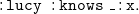
(1) \begin{equation} \mathtt {:lucy\;\;:knows\;\;:tom.} \end{equation}

means ³ that “lucy knows tom.” Sets of triples are interpreted as their conjunction. Like RDF, $N_3$ supports blank nodes, usually starting with _:, which stand for (implicitly) existentially quantified variables. The statement

(2) \begin{equation} \mathtt {:lucy\;\;:knows\;\;\_:x.} \end{equation}

means “there exists someone who is known by lucy.” $N_3$ furthermore supports implicitly universally quantified variables, indicated by a leading question mark (?), and implications which are stated using graphs, i.e., sets of triples, surrounded by curly braces ({}) as body and head connected via an arrow (= >). The formula

(3) \begin{equation} \mathtt {\{:lucy\;\;:knows\;\;?x\}= \gt \{?x\;\;:knows\;\;:lucy\}.} \end{equation}

means that “everyone known by Lucy also knows her.” Furthermore, $N_3$ allows the use of blank nodes in rules. These blank nodes are not quantified outside the rule like the universal variables, but in the rule part they occur in, that is either in its body or its head.

(4) \begin{equation} \mathtt {\{?x\;\;:knows\;\;:tom\}= \gt \{?x\;\;:knows\;\;\_:y.\;\;\_:y\;\;:name\;\;"Tom"\}.} \end{equation}

means “everyone knowing Tom knows someone whose name is Tom.”

This last example shows, that $N_3$ supports rules concluding the existence of certain terms which makes it easy to express them as existential rules. An existential rule is a first-order sentence of the form

(5) \begin{equation} \forall \mathbf{x}, \mathbf{y} .\,\varphi [\mathbf{x}, \mathbf{y}] \rightarrow \exists \mathbf{z} .\,\psi [\mathbf{y}, \mathbf{z}] \end{equation}

where $\mathbf{x}, \mathbf{y}, \mathbf{z}$ are mutually disjoint lists of variables, $\varphi$ and $\psi$ are conjunctions of atoms using only variables from the given lists, and $\varphi$ is referred to as the body of the rule while $\psi$ is called the head. Using the basic syntactic shape of (5) we go through all the example $N_3$ formulae (1)–(4) again and represent them as existential rules. To allow for the full flexibility of $N_3$ and RDF triples, we translate each RDF triple, just like the one in (1) into a first-order atom ${\textit {tr}}(\mathtt {:lucy}, \mathtt {:knows}, \mathtt {:tom})$ . Here, $\textit {tr}$ is a ternary predicate holding subject, predicate, and object of a given RDF triple. This standard translation makes triple predicates (e.g., $\mathtt {:knows}$ ) accessible as terms. First-order atoms are also known as facts, finite sets of facts are called databases, and (possibly infinite) sets of facts are called instances. Existential rules are evaluated over instances (cf. Section 4).

Compared to other rule languages, the distinguishing feature of existential rules is the use of existentially quantified variables in the head of rules (cf. $\mathbf{z}$ in (5)). The $N_3$ formula in (2) contains an existentially quantified variable and can, thus, be encoded as

(6) \begin{equation} \rightarrow \exists x.\ {\textit {tr}}(\mathtt {:lucy}, \mathtt {:knows}, x) \end{equation}

Rule (6) has an empty body, which means the head is unconditionally true. Rule (6) is satisfied on instances containing any fact ${\textit {tr}}(\mathtt {:lucy},\mathtt {:knows},\_)$ (e.g., ${\textit {tr}}(\mathtt {:lucy},\mathtt {:knows},\mathtt {:tim})$ so that variable $x$ can be bound to $\mathtt {:tim}$ ).

The implication of (3) has

(7) \begin{equation} \forall x .\ {\textit {tr}}(\mathtt {:lucy},\mathtt {:knows},x) \rightarrow {\textit {tr}}(x, \mathtt {:knows}, \mathtt {:lucy}) \end{equation}

as its (existential) rule counterpart, which does not contain any existentially quantified variables. Rule (7) is satisfied in the instance

\begin{equation*}{{\mathcal{I}}}_{1} = \{ {\textit {tr}}(\mathtt {:lucy}, \mathtt {:knows}, \mathtt {:tom}), {\textit {tr}}(\mathtt {:tom}, \mathtt {:knows},\mathtt {:lucy}) \}\end{equation*}

but not in

\begin{equation*}{\mathcal{K}}_{1} = \{ {\textit {tr}}(\mathtt {:lucy}, \mathtt {:knows}, \mathtt {:tom}) \}\end{equation*}

since the only fact in ${\mathcal{K}}_1$ matches the body of the rule, but there is no fact reflecting on its (instantiated) head (i.e., the required fact ${\textit {tr}}(\mathtt {:tom},\mathtt {:knows},\mathtt {:lucy})$ is missing). Ultimately, the implication (4) with blank nodes in its head may be transferred to a rule with an existential quantifier in the head:

(8) \begin{equation} \forall x.\ {\textit {tr}}(x, \mathtt {:knows}, \mathtt {:tom}) \rightarrow \exists y .\ \left ({\textit {tr}}(x, \mathtt {:knows}, y) \wedge {\textit {tr}}(y, \mathtt {:name}, \mathtt {"Tom"})\right )\text . \end{equation}

It is clear that rule (8) is satisfied in instance

\begin{equation*}{{\mathcal{I}}}_{2} = \{ {\textit {tr}}(\mathtt {:lucy},\mathtt {:knows},\mathtt {:tom}), {\textit {tr}}(\mathtt {:tom}, \mathtt {:name}, \mathtt {"Tom"}) \}\text .\end{equation*}

However, instance ${\mathcal{K}}_1$ does not satisfy rule (8) because although the only fact satisfies the rule’s body, there are no facts jointly satisfying the rule’s head.

Note, for query answering over databases and rules, it is usually not required to decide for a concrete value of $y$ (in rule (8)). Many implementations, therefore, use some form of abstraction: for instance, Skolem terms. VLog and Nemo implement the standard chase which uses another set of terms, so-called labeled nulls. Instead of injecting arbitrary constants for existentially quantified variables, (globally) fresh nulls are inserted in the positions existentially quantified variables occur. Such a labeled null embodies the existence of a constant on the level of instances (just like blank nodes in RDF graphs). Let $n$ be such a labeled null. Then ${{\mathcal{I}}}_{2}$ can be generalized to

\begin{equation*}{{\mathcal{I}}}_{3} = \{ {\textit {tr}}(\mathtt {:lucy},\mathtt {:knows},\mathtt {:tom}), {\textit {tr}}(\mathtt {:lucy},\mathtt {:knows},n), {\textit {tr}}(n, \mathtt {:name}, \mathtt {"Tom"}) \}\text ,\end{equation*}

on which rule (8) is satisfied, binding null $n$ to variable $y$ . ${{\mathcal{I}}}_{3}$ is, in fact, more general than ${{\mathcal{I}}}_{2}$ by the following observation: There is a mapping from ${{\mathcal{I}}}_{3}$ to ${{\mathcal{I}}}_{2}$ that is a homomorphism (see Subsection 4.1 for a formal introduction) but not vice versa. The homomorphism here maps the null $n$ (from ${{\mathcal{I}}}_{3}$ ) to the constant $\mathtt {:tom}$ (in ${\mathcal{I}}_{2}$ ). Intuitively, the existence of a query answer (for a conjunctive query) on ${\mathcal{I}}_{3}$ implies the existence of a query answer on ${\mathcal{I}}_{2}$ . Existential rule reasoners implementing some form of the chase aim at finding the most general instances (universal models) in this respect (Deutsch et al. 2008).

In the remainder of this paper, we further analyze the relation between $N_3$ and existential rules. First, we give a brief formal account of the two languages and then provide a correct translation function from $N_3$ to existential rules.

3 Existential N3

In the previous section we introduced essential elements of $N_3$ , namely triples and rules. $N_3$ also supports more complex constructs like lists, nesting of rules, and quotation. As these features are not covered by existential rules, we define a subset of $N_3$ excluding them, called existential $N_3$ ( ${N_3}^\exists$ ). This fragment of $N_3$ is still very powerful as it covers ontology mapping, one of N3’s main use cases. Many ontologies rely on patterns including auxiliary blank nodes. ${N_3}^\exists$ supports the production of these. ⁴ In practice, these mappings are often connected with build-in functions like calculations or string operations, ⁵ these are not covered yet, but could be added. A more difficult feature to add would be the support of so-called rule-producing rules: In N3 it is possible to nest rules into the head of other rules. While this technique does not yield more expressivity, it is commonly used to translate from RDF datasets to N3 rules (see e.g., Arndt et al. 2016). Such rule-producing rules can not be covered by existential rules as these only allow the derivation of facts.

We base our definitions on so-called simple $N_3$ formulae (Arndt 2019, Chapter 7), these are $N_3$ formulae which do not allow for nesting.

3.1 Syntax

${N_3}^\exists$ relies on the RDF alphabet. As the distinction is not relevant in our context, we consider IRIs and literals together as constants. Let $C$ be a set of such constants, $U$ a set of universal variables (starting with ?), and $E$ a set of existential variables (i.e., blank nodes). If the sets $C$ , $U$ , $E$ , and $\{\mathtt {\{}, \mathtt {\}}, \mathtt {= \gt }, \mathtt {.}\}$ are mutually disjoint, we call $\mathfrak{A}:=C \,\cup \, U \,\cup \, E \,\cup \, \{\mathtt {\{}, \mathtt {\}}, \mathtt {= \gt }, \mathtt {.}\}$ an $N_3$ alphabet. Figure 1 provides the syntax of ${N_3}^\exists$ over $\mathfrak{A}$ .

Fig. 1. Syntax of $\operatorname {N3}^\exists$ .

${N_3}^\exists$ fully covers RDF. RDF formulae are conjunctions of atomic formulae. Just as generalized RDF (Cyganiak et al. 2014), ${N_3}^\exists$ allows for literals and blank nodes to occur in subject, predicate, and object position. The same holds for universal variables which are not present in RDF. This syntactical freedom is inherited from full N3 and makes it possible to – among other things – express the rules for RDF/S (Hayes and Patel-Schneider 2014, Appendix A) and OWL-RL (Motik et al. 2009, Section 4.3) entailment via N3. As an example for that, consider the following rule ⁶ for inverse properties:

(9) \begin{equation} \mathtt {\{?p1\;\;owl:inverseOf\;\;?p2\;\;.\;\;?x\;\;?p1\;\;?y\;\;.\}= \gt \{?y\;\;?p2\;\;?x \}.} \end{equation}

If we apply this rule on triple (1) in combination with

(10) \begin{equation} \mathtt {:knows\;\;owl:inverseOf\;\;:isKnownBy.} \end{equation}

we derive

(11) \begin{equation} \mathtt {:tom\;\;:isKnownBy\;\;:lucy.} \end{equation}

Similar statements and rules can be made for triples including literals. We can for example declare that the :name from rule (4) is the owl:inverseOf of :isNameOf. ⁷ With rule (10) we then derive from

(12) \begin{equation} \mathtt {\_:x\;\;:name\;\;"Tom".} \end{equation}

that

(13) \begin{equation} \mathtt {"Tom"\;\;:isNameOf\;\;\_:x.} \end{equation}

In that sense the use of generalized RDF ensures that all logical consequences we are able to produce via rules can also be stated in the language. This principle of syntactical completeness is also the reason to allow literals and blank nodes in predicate position. As universals may occur in predicate position, this also needs to be the case for all other kinds of symbols.

Currently, there is one exception to our principle: The syntax above allows rules having new universal variables in their head like for example

(14) \begin{equation} \mathtt {\{:lucy\;\;:knows\;\;:tom\}= \gt \{?x\;\;:is\;\;:happy\}.} \end{equation}

which results in a rule expressing “if lucy knows tom, everyone is happy.” This implication is problematic: Applied on triple (1), it yields $\mathtt {? x\;\;:is\;\;:happy.}$ which is a triple containing a universal variable. Such triples are not covered by our syntax, the rule thus introduces a fact we cannot express. Therefore, we restrict ${N_3}^\exists$ rules to well-formed implications which rely on components. Components can be seen as direct parts ⁸ an N3 formula consists of. Let $f$ be a formula or an expression over an alphabet $\mathfrak{A}$ . The set ${\operatorname {comp}}(f)$ of components of $f$ is defined as:

• • If $f$ is an atomic formula or a triple expression of the form $t_1\, t_2\, t_3.$ , ${\operatorname {comp}}(f)=\{t_1,t_2,t_3\}$ .

• • If $f$ is an implication of the form $\mathtt {{e_{1}}= \gt {e_{2}}}.$ , then ${\operatorname {comp}}(f)=\{\mathtt {{e_1}, {e_2}}\}$ .

• • If $f$ is a conjunction of the form $f_1 f_2$ , then ${\operatorname {comp}}(f)={\operatorname {comp}}(f_1)\cup {\operatorname {comp}}(f_2)$ .

A rule $\mathtt {\{e}_1\mathtt {\}= \gt \{e}_2\mathtt {\}} .$ is called well-formed if $({\operatorname {comp}}(\mathtt {e}_2)\setminus {\operatorname {comp}}(\mathtt {e}_1))\cap U=\emptyset$ . For the remainder of this paper we assume all implications to be well-formed. Note that this definition of well-formed formulae is closely related to the idea of safety in logic programing. Well-formed rules are safe.

3.2 Semantics

In order to define the semantics of ${N_3}^\exists$ we first note, that in our fragment of $N_3$ all quantification of variables is only defined implicitly. The blank node in triple (2) is understood as an existentially quantified variable, the universal in formula (3) as universally quantified. Universal quantification spans over the whole formula – variable ?x occurring in body and head of rule (3) is universally quantified for the whole implication – while existential quantification is local – the conjunction in the head of rule (4) is existentially quantified there. Adding new triples as conjuncts to formula (4) like

(15) \begin{equation} \mathtt {:lucy\;\;:knows\;\;\_:y.\;\;\_:y\;\;:likes\;\;:cake. } \end{equation}

leads to the new statement that “lucy knows someone who likes cake” but even though we are using the same blank node identifier _:y in both formulae, the quantification of the variables in this formula is totally seperated and the person named “Tom” is not necessarily related to the cake-liker. With the goal to deal with this locality of blank node scoping, we define substitutions which are only applied on components of formulae and leave nested elements like for example the body and head of rule (3) untouched.

A substitution $\sigma$ is a mapping from a set of variables $X\subset U\cup E$ to the set of $N_3$ terms. We apply $\sigma$ to a term, formula or expression $x$ as follows:

• • $x \sigma = \sigma (x)$ if $x\in X$ ,

• • $(s\,p\,o) \sigma =(s\sigma )( p\sigma ) (o\sigma )$ if $x=s\,p\, o$ is an atomic formula or a triple expression,

• • $(f_1f_2) \sigma =(f_1\sigma )( f_2\sigma )$ if $x=f_1f_2$ is a conjunction,

• • $x \sigma = x$ else.

For formula $f=\mathtt {\_:x\;\;:p\;\;:o. \{\_:x\;\;:b\;\;:c\}= \gt \{\_:x\;\;:d\;\;:e\}.}$ , substitution $\sigma$ and $\mathtt {\_:x}\in \text{dom}(\sigma )$ , we get: $f\sigma =\sigma (\mathtt {\_:x}) \mathtt {:p\;\;:o. \{\_:x\;\;:b\;\;:c\}= \gt \{\_:x\;\;:d\;\;:e\}}$ . ⁹ We use the substitution to define the semantics of ${N_3}^\exists$ which additionally makes use of N3 interpretations $\mathfrak{I} = (\mathfrak{D},\mathfrak{a},\mathfrak{p})$ consisting of (1) a set $\mathfrak{D}$ , called the domain of $\mathfrak{I}$ ; (2) a mapping $\mathfrak{a}: C\rightarrow \mathfrak{D}$ , called the object function; (3) a mapping $\mathfrak{p}: \mathfrak{D} \rightarrow 2^{\mathfrak{D} \times \mathfrak{D}}$ , called the predicate function.

Just as the function IEXT in RDF’s simple interpretations (Hayes 2004), $N_3$ ’s predicate function maps elements from the domain of discourse to a set of pairs of domain elements and is not applied on relation symbols directly. This makes quantification over predicates possible while not exceeding first-order logic in terms of complexity. To introduce the semantics of ${N_3}^\exists$ , let $\mathfrak{I}=(\mathfrak{D},\mathfrak{a,p})$ be an $N_3$ interpretation. For an ${N_3}^\exists$ formula $f$ :

1. 1. If $W=\text{comp}(f)\cap E \neq \emptyset$ , then $\mathfrak{I}\models f$ iff $\mathfrak{I}\models f\mu$ for some substitution $\mu \;:\; W\rightarrow C$ .

2. 2. If $\text{comp}(f)\cap E=\emptyset$ :

1. (a) If $f$ is an atomic formula $t_1\, t_2\, t_3$ , then $\mathfrak{I} \models t_1\, t_2\, t_3$ . iff $(\mathfrak{a}(t_1),\mathfrak{a}(t_3))\in \mathfrak{p}(\mathfrak{a}(t_2))$ .

2. (b) If $f$ is a conjunction $f_1f_2$ , then $\mathfrak{I}\models f_1 f_2$ iff $\mathfrak{I}\models f_1$ and $\mathfrak{I}\models f_2$ .

3. (c) If $f$ is an implication, then $\mathfrak{I} \models \mathtt {{ e_1 } = \gt {e_2}}$ iff $\mathfrak{I} \models e_2\sigma$ if $\mathfrak{I} \models e_1\sigma$ for all substitutions $\sigma$ on the universal variables $\text{comp}(\mathtt {e}_1)\cap U$ by constants.

The semantics as defined above uses a substitution into the set of constants instead of a direct assignment to the domain of discourse to interpret quantified variables. This design choice inherited from $N_3$ ensures referential opacity of quoted graphs and means, in essence, that quantification always refers to named domain elements.

With that semantics, we call an interpretation $\mathfrak{M}$ model of a dataset $\Phi$ , written as $\mathfrak{M}\models \Phi$ , if $\mathfrak{M}\models f$ for each formula $f\in \Phi$ . We say that two sets of ${N_3}^\exists$ formulae $\Phi$ and $\Psi$ are equivalent, written as $\Phi \equiv \Psi$ , if for all interpretations $\mathfrak{M}$ : $\mathfrak{M}\models \Phi$ iff $\mathfrak{M}\models \Psi$ . If $\Phi =\{\phi \}$ and $\Psi =\{\psi \}$ are singleton sets, we write $\phi \equiv \psi$ omitting the brackets.

3.2.1 Piece normal form

${N_3}{}^\exists$ formulae consist of conjunctions of triples and implications. For our goal of translating such formulae to existential rules, it is convenient to consider sub-formulae seperately.

Below, we therefore define the so-called Piece Normal Form (PNF) for ${N_3}{}^\exists$ formulae and show that each such formula $f$ is equivalent to a set of sub-formulae $\Phi$ (i.e., $\Phi \equiv \phi$ ) in PNF. We proceed in two steps. First, we separate formulae based on their blank node components. If two parts of a conjunction share a blank node component, as in formula (15), we cannot split the formula into two since the information about the co-reference would get lost. However, if conjuncts either do not contain blank nodes or only contain disjoint sets of these, we can split them into so-called pieces: Two formulae $f_1$ and $f_2$ are called pieces of a formula $f$ if $f=f_1f_2$ and ${\operatorname {comp}}(f_1)\cap {\operatorname {comp}}(f_2)\cap E=\emptyset$ . For such formulae we know:

Lemma 3.1 (Pieces). Let $f=f_1f_2$ be an ${N_3}^\exists$ conjunction and let ${\operatorname {comp}}(f_1)\cap {\operatorname {comp}}(f_2)\cap E=\emptyset$ , then for each interpretation $\mathfrak{I}$ , $\mathfrak{I}\models f \text{ iff } \mathfrak{I}\models f_1 \text{ and } \mathfrak{I}\models f_2$ .

Proof.

1. 1. If ${\operatorname {comp}}(f)\cap E=\emptyset$ the claim follows immediately by point 2b in the semantics definition.

2. 2. If $W=\text{comp}(f)\cap E \neq \emptyset$ : ( $\Rightarrow$ ) If $\mathfrak{I}\models f$ then there exists a substitution $\mu \;:\;{\operatorname {comp}}(f)\cap E\rightarrow C$ such that $\mathfrak{I}\models f\mu$ , that is $\mathfrak{I}\models (f_1\mu )\,(f_2\mu )$ . According to the previous point that implies $\mathfrak{I}\models f_1\mu$ and $\mathfrak{I}\models f_2\mu$ and thus $\mathfrak{I}\models f_1$ and $\mathfrak{I}\models f_2$ . ( $\Leftarrow$ ) If $\mathfrak{I}\models f_1$ and $\mathfrak{I}\models f_2$ , then there exist two substitutions $\mu _1:{\operatorname {comp}}(f_1)\cap E\rightarrow C$ and $\mu _2:{\operatorname {comp}}(f_2)\cap E\rightarrow C$ such that $\mathfrak{I}\models f_1\mu _1$ and $\mathfrak{I}\models f_2\mu _2$ . As the domains of the two substitutions are disjoint (by assumption), we can define the substitution $\mu \;:\;{\operatorname {comp}}(f)\cap E\rightarrow C$ as follows:

   \begin{align*} \mu (v) = {\begin{cases} \mu _1(v) & \text{ if } v\in {\operatorname {comp}}(f_1) \\ \mu _2(v)& \, \text{else}\\ \end{cases}} \end{align*}
   Then $\mathfrak{I}\models f\mu$ and therefore $\mathfrak{I}\models f$ .

If we recursively divide all pieces into sub-pieces, we get a maximal set $F=\{f_1, f_2, \ldots , f_n\}$ for each formula $f$ such that $F\equiv \{f\}$ and for all $1 \leq i, j \leq n$ , $\text{comp}(f_{i})\cap \text{comp}(f_{j})\cap E \neq \emptyset$ implies $i=j$ .

Second, we replace all blank nodes occurring in rule bodies by fresh universals. The rule

\begin{equation*}\mathtt {\{\_:x\;\;:likes\;\;:cake\}= \gt \{:cake\;\;:is\;\;:good\}.}\end{equation*}

becomes

\begin{equation*}\mathtt {\{?y\;\;:likes\;\;:cake\}= \gt \{:cake\;\;:is\;\;:good\}.}\end{equation*}

Note that both rules have the same meaning, namely “if someone likes cake, then cake is good.” We generalize that:

Lemma 3.2 (Eliminating Existentials). Let $f= \mathtt {{e_1} = \gt { e_2}}$ and $g=\mathtt {{ e'_1 } = \gt { e_2}}$ be ${N_3}^\exists$ implications such that $e'_1=e_1\sigma$ for some injective substitution $\sigma \;:\;{\operatorname {comp}}(e_1)\cap E\rightarrow U\setminus {\operatorname {comp}}(e_1)$ of the existential variables of $e_1$ by universals. Then $f\equiv g$ .

Proof. We first note that ${\operatorname {comp}}(f)\cap E=\emptyset$ and ${\operatorname {comp}}(g)\cap E=\emptyset$ since both formulae are implications.

( $\Rightarrow$ ) We assume that $\mathfrak{M}\not \models g$ for some model $\mathfrak{M}$ . That is, there exists a substitution $\nu \;:\; ({\operatorname {comp}}(e'_1)\cup {\operatorname {comp}}(e_2))\cap U\rightarrow C$ such that $\mathfrak{M}\models e'_1 \nu$ and $\mathfrak{M}\not \models e_2\nu$ . We show that $\mathfrak{M}\models e_1\nu$ : As $(({\operatorname {comp}}(e_1)\cup {\operatorname {comp}}(e_2))\cap U)\subset (({\operatorname {comp}}(e'_1)\cup {\operatorname {comp}}(e_2))\cap U)$ , we know that ${\operatorname {comp}}(e_1\nu )\cap U =\emptyset$ . With the substitution $\mu := \nu \circ \sigma$ for the existential variables in $e_1\nu$ we get $\mathfrak{M}\models (e_1 \nu ) \sigma$ and thus $\mathfrak{M}\models (e_1 \nu )$ , but as $\mathfrak{M}\not \models (e_2 \nu )$ we can conclude that $\mathfrak{M}\not \models f$ .

( $\Leftarrow$ ) We assume that $\mathfrak{M}\not \models f$ . That is, there exists a substitution $\nu \;:\; ({\operatorname {comp}}(e_1)\cup {\operatorname {comp}}(e_2))\cap U\rightarrow C$ such that $\mathfrak{M}\models e_1 \nu$ and $\mathfrak{M}\not \models e_2\nu$ . As $\mathfrak{M}\models e_1 \nu$ , there exists a substitution $\mu \;:\;{\operatorname {comp}}(e_1\nu )\cap E\rightarrow C$ such that $\mathfrak{M}\models (e_1 \nu )\mu$ . With that we define a substitution $\nu ':({\operatorname {comp}}(e_1)\cup {\operatorname {comp}}(e_2))\cap U\rightarrow C$ as follows: $\nu ':U\rightarrow C$ as follows:

\begin{equation*}\nu '(v) = \begin{cases} \mu (\sigma ^{-1}(v)) & \text{ if } v\in range(\sigma ) \\ \nu (v)& \, \text{else} \end{cases}\end{equation*}

With that substitution we get $\mathfrak{M}\models e'_1\nu '$ but $\mathfrak{M}\not \models e_2\nu '$ and thus $\mathfrak{M}\not \models g$ .

For a rule $f$ we call the formula $f'$ in which all existentials occurring in its body are replaced by universals following Lemma 3.2 the normalized version of the rule. We call an ${N_3}{}^{\exists }$ formula $f$ normalized, if all rules occurring in it as conjuncts are normalized. Combining the findings of the two previous lemmas, we introduce the Piece Normal Form:

Definition 3.3 (Piece Normal Form). A finite set $\Phi = { f_1, f_2, \ldots , f_n }$ of ${N_3}{}^\exists$ formulae is in piece normal form (PNF) if all $f_i \in \Phi$ ( $1 \leq i \leq n$ ) are normalized and $n \in \mathbb{N}$ is the maximal number such that for $1 \leq i,j \leq n$ , ${\operatorname {comp}}(f_i) \cap {\operatorname {comp}}(f_j) \cap E \neq \emptyset$ implies $i = j$ . If $f_i \in \Phi$ is a conjunction of atomic formulae, we call $f_i$ an atomic piece.

We get the following result for ${N_3}^\exists$ formulae:

Theorem 3.4. For every well-formed ${N_3}^\exists$ formula $f$ , there exists a set $F =\{ f_{1}, f_{2}, \ldots , f_{k}\}$ of ${N_3}^\exists$ formulae such that $F\equiv \{f\}$ and $F$ is in piece normal form.

Proof. The claim follows immediately from Lemma 3.1 and Lemma 3.2.

Since the piece normal form $F$ of ${N_3}^\exists$ formula $f$ is obtained by only replacing variables and separating conjuncts of $f$ into the set form, the overall size of $F$ is linear in $f$ .

4 From N3 to existential rules

Due to Theorem3.4, we translate sets $F$ of ${N_3}^\exists$ formulae in PNF (cf. Definition 3.3) to sets of existential rules $\mathcal{T}(F)$ without loss of generality. As a preliminary step, we introduce the language of existential rules formally. Later on, we explain and formally define the translation function already sketched in Section 2. We close this section with a correctness argument, paving the way for existential rule reasoning for ${N_3}^\exists$ formulae.

4.1 Foundations of existential rule reasoning

As for $N_3$ , we consider a first-order vocabulary, consisting of countably infinite mutually disjoint sets of constants ( $\mathbf{C}$ ), variables ( $\mathbf{V}$ ), and additionally so-called (labeled) nulls ( $\mathbf{N}$ ). ¹⁰ As already mentioned in Section 2, we use the same set of constants as $N_3$ formulae, meaning ${\mathbf{C}} = C$ . Furthermore, let $\mathbf{P}$ be a (countably infinite) set of relation names, where each $p\in {\mathbf{P}}$ comes with an arity $\mathit{ar}(p)\in \mathbb{N}$ . $\mathbf{P}$ is disjoint from the term sets $\mathbf{C}$ , $\mathbf{V}$ , and $\mathbf{N}$ . We reserve the ternary relation name ${\textit {tr}}\in {\mathbf{P}}$ for our encoding of $N_3$ triples. If $p\in {\mathbf{P}}$ and $t_{1},t_{2},\ldots ,t_{\mathit{ar}(p)}$ is a list of terms (i.e., each $t_{i}\in {\mathbf{C}}\cup {\mathbf{N}}\cup {\mathbf{V}}$ ), $p(t_{1},t_{2},\ldots ,t_{\mathit{ar}(p)})$ is called an atom. We often use $\mathbf{t}$ to summarize a term list like $t_{1},\ldots ,t_{n}$ ( $n\in \mathbb{N}$ ), and treat it as a set whenever order is irrelevant. An atom $p(\mathbf{t})$ is ground if $\mathbf{t} \subseteq {\mathbf{C}}$ . An instance is a (possibly infinite) set $\mathcal{I}$ of variable-free atoms and a finite set of ground atoms ${\mathcal{D}}$ is called a database.

For a set of atoms ${\mathcal{I}}[A]$ and an instance $\mathcal{I}$ , we call a function $h$ from the terms occurring in ${\mathcal{I}}[A]$ to the terms in $\mathcal{I}$ a homomorphism from ${\mathcal{I}}[A]$ to $\mathcal{I}$ , denoted by $h \;:\; {\mathcal{I}}[A]\to {\mathcal{I}}$ , if (1) $h(c)=c$ for all $c\in {\mathbf{C}}$ (occurring in ${\mathcal{I}}[A]$ ), and (2) $p(\mathbf{t})\in {\mathcal{I}}[A]$ implies $p(h(\mathbf{t}))\in {\mathcal{I}}$ . If any homomorphism from ${\mathcal{I}}[A]$ to $\mathcal{I}$ exists, write ${\mathcal{I}}[A]\to {\mathcal{I}}$ . Please note that if $n$ is a null occurring in ${\mathcal{I}}[A]$ , then $h(n)$ may be a constant or null.

For an (existential) rule $r\colon \forall \mathbf{x}, \mathbf{y} .\ \varphi [\mathbf{x},\mathbf{y}] \rightarrow \exists \mathbf{z} .\ \psi [\mathbf{y},\mathbf{z}]$ (cf. (5)), rule body ( ${\textsf {body}(r)} := \varphi$ ) and head ( ${\textsf {head}(r)} := \psi$ ) will also be considered as sets of atoms for a more compact representation of the semantics. The notation $\varphi [\mathbf{x},\mathbf{y}]$ ( $\psi [\mathbf{y},\mathbf{z}]$ , resp.) indicates that the only variables occurring in $\varphi$ ( $\psi$ , resp.) are $\mathbf{x}\cup \mathbf{y}$ ( $\mathbf{y}\cup \mathbf{z}$ , resp.). A finite set of existential rules $\Sigma$ is called an (existential) rule program.

Let $r$ be a rule and $\mathcal{I}$ an instance. We call a homomorphism $h \;:\; {\textsf {body}(r)} \to {\mathcal{I}}$ a match for $r$ in $\mathcal{I}$ . Match $h$ is satisfied for $r$ in $\mathcal{I}$ if there is an extension $h^{\star }$ of $h$ (i.e., $h\subseteq h^{\star }$ ) such that $h^{\star }({\textsf {head}(r)})\subseteq {\mathcal{I}}$ . If all matches of $r$ are satisfied in $\mathcal{I}$ , we say that r is satisfied in $\mathcal{I}$ , denoted by ${\mathcal{I}}\models r$ . For a rule program $\Sigma$ and database ${\mathcal{D}}$ , instance $\mathcal{I}$ is a model of $\Sigma$ and ${\mathcal{D}}$ , denoted by ${\mathcal{I}} \models \Sigma ,{\mathcal{D}}$ , if ${\mathcal{D}}\subseteq {\mathcal{I}}$ and ${\mathcal{I}}\models r$ for each $r\in \Sigma$ .

Labeled nulls play the role of fresh constants without further specification, just like blank nodes in RDF or $N_3$ . The chase is a family of algorithms that soundly produces models of rule programs by continuously applying rules for unsatisfied matches. Rule heads are then instantiated and added to the instance. Existentially quantified variables are thereby replaced by (globally) fresh nulls in order to facilitate arbitrary constant injections. More formally, we call a sequence ${\mathcal{D}}^0 {\mathcal{D}}^1 {\mathcal{D}}^2 \ldots$ a chase sequence of rule program $\Sigma$ and database ${\mathcal{D}}$ if (1) ${\mathcal{D}}^0 = {\mathcal{D}}$ and (2) for $i \gt 0$ , ${\mathcal{D}}^i$ is obtained from ${\mathcal{D}}^{i-1}$ by applying a rule $r\in \Sigma$ for match $h$ in ${\mathcal{D}}^{i-1}$ (i.e., $h \;:\; {\textsf {body}(r)} \to {\mathcal{D}}^{i-1}$ is an unsatisfied match and ${\mathcal{D}}^i = {\mathcal{D}}^{i-1} \cup \{ h^{\star }({\textsf {head}(r)}) \}$ for an extension $h^{\star }$ of $h$ ). The chase of $\Sigma$ and ${\mathcal{D}}$ is the limit of a chase sequence ${\mathcal{D}}^0 {\mathcal{D}}^1 {\mathcal{D}}^2 \ldots$ , that is $\bigcup _{i\geq 0} {\mathcal{D}}^0$ . Although chase sequences are not necessarily finite, ¹¹ the chase always is a (possibly infinite) model ¹² (Deutsch et al. 2008). The described version of the chase is called standard chase or restricted chase.

We say that two rule programs $\Sigma _{1}$ and $\Sigma _{2}$ are equivalent, denoted $\Sigma _{1} {\mathrel {\leftrightarrows }} \Sigma _{2}$ , if for all instances $\mathcal{I}$ , ${\mathcal{I}}\models \Sigma _{1}$ if and only if ${\mathcal{I}}\models \Sigma _{2}$ . Equivalences of existential rules have been extensively studied in the framework of data exchange (Fagin et al. 2008; Pichler et al. 2011). Our equivalence is very strong and is called logical equivalence in the data exchange literature. For an alternative equivalence relation between rule programs, we could have equally considered equality of ground models (i.e., those models that are null-free). Let us define this equivalence as follows: $\Sigma _{1} {\mathrel {\leftrightarrows }}_{g} \Sigma _{2}$ if for each ground instance $\mathcal{I}$ , ${\mathcal{I}}\models \Sigma _{1}$ if and only if ${\mathcal{I}}\models \Sigma _{2}$ . The following lemma helps simplifying the proofs concerning the correctness of our transformation ¹³ function later on.

Lemma 4.1. $\mathrel {\leftrightarrows }$ and ${\mathrel {\leftrightarrows }}_{g}$ coincide.

Proof. Of course, ${\mathrel {\leftrightarrows }}\subseteq {\mathrel {\leftrightarrows }}_{g}$ holds since since the set of all ground models of a rule program is a subset of all models of that program.

Towards showing ${\mathrel {\leftrightarrows }}_{g}\subseteq {\mathrel {\leftrightarrows }}$ , assume rule programs $\Sigma _{1}$ and $\Sigma _{2}$ such that $\Sigma _{1}{\mathrel {\leftrightarrows }}_{g}\Sigma _{2}$ , but . Then there is a model ${\mathcal{I}}[M]$ of $\Sigma _{1}$ , such that (or vice versa), implying that for some rule $r\in \Sigma _{2}$ there is a match $h$ in ${\mathcal{I}}[M]$ but for no extension $h^{\star }$ , we get $h^{\star }({\textsf {head}(r)})\subseteq {\mathcal{I}}[M]$ . As $\Sigma _{1}{\mathrel {\leftrightarrows }}_{g} \Sigma _{2}$ , ${\mathcal{I}}[M]$ cannot be a ground instance and, thus, contains at least one null.

Claim: Because of ${\mathcal{I}}[M]$ , there is a ground instance ${\mathcal{I}}[M]_{g}$ , such that ${\mathcal{I}}[M]_{g}\models \Sigma _{1}$ and . But then ${\mathcal{I}}[M]_{g}$ constitutes a counterexample to the assumption that $\Sigma _{1}{\mathrel {\leftrightarrows }}_{g} \Sigma _{2}$ . Thus, the assumption would be disproven.

In order to show the claim, we construct ${\mathcal{I}}[M]_{g}$ from ${\mathcal{I}}[M]$ by replacing every null $n$ in ${\mathcal{I}}[M]$ by a (globally) fresh constant $c_{n}$ . Since there might not be enough constants – ${\mathcal{I}}[M]$ may already use all countably infinite constants $c\in {\mathbf{C}}$ – we take a little detour: although the set of constants in use might be infinite in ${\mathcal{I}}[M]$ , the number of constants used inside the rule programs $\Sigma _{1}$ and $\Sigma _{2}$ is finite. ¹⁴ Create instance ${\mathcal{I}}[M]''$ from ${\mathcal{I}}[M]$ by replacing all constants $c$ not part of $\Sigma _{1}$ or $\Sigma _{2}$ by fresh nulls $n_{c}$ . Once again, ${\mathcal{I}}[M]$ may already use up all nulls $n\in {\mathbf{N}}$ . So we have to take yet another detour from ${\mathcal{I}}[M]$ to ${\mathcal{I}}[M]'$ as follows:

Let $\gamma \;:\; {\mathbf{N}}\to \mathbb{N}$ be a (necessarily injective) enumeration of $\mathbf{N}$ . Define $\eta \;:\; {\mathbf{C}}\cup {\mathbf{N}}\to {\mathbf{C}}\cup {\mathbf{N}}$ by (1) $\eta (c):=c$ for all $c\in {\mathbf{C}}$ and (2) $\eta (n):= \eta ^{-1}(2\cdot \eta (n))$ . Then ${\mathcal{I}}[M]'$ is produced by applying $\eta$ to ${\mathcal{I}}[M]$ . Note, for each number $k\in \mathbb{N}$ , $\eta ^{-1}(2k+1)$ is not a null in ${\mathcal{I}}[M]'$ . Since $\eta$ is an isomorphism between ${\mathcal{I}}[M]$ and ${\mathcal{I}}[M]'$ , we get that ${\mathcal{I}}[M]\models \Sigma$ if and only if ${\mathcal{I}}[M]'\models \Sigma$ for all rule programs $\Sigma$ . Recall that isomorphic models preserve all first-order sentences (see, e.g., Ebbinghaus et al. 1994). Hence, ${\mathcal{I}}[M]'\models \Sigma _{1}$ and .

Next we construct ${\mathcal{I}}[M]''$ from ${\mathcal{I}}[M]'$ by function $\omega$ mapping the terms occurring in ${\mathcal{I}}[M]'$ to ${\mathbf{C}}\cup {\mathbf{N}}$ , such that (1) $\omega (c)=c$ if $c$ is a constant occurring in $\Sigma _{1}\cup \Sigma _{2}$ , (2) $\omega (d)$ is a fresh null $n_{d}$ if $d$ is a constant not occurring in $\Sigma _{1}\cup \Sigma _{2}$ , and (3) $\omega (n)=n$ otherwise. $\omega$ exists because the number of nulls in use by ${\mathcal{I}}[M]'$ is countably infinite. Note that $\omega$ is injective and $\omega ({\mathcal{I}}[M]')={\mathcal{I}}[M]''$ uses only finitely many constants. Once again we show that ${\mathcal{I}}[M]'\models \Sigma$ if and only if ${\mathcal{I}}[M]''\models \Sigma$ for arbitrary rule programs $\Sigma$ , implying that ${\mathcal{I}}[M]''\models \Sigma _{1}$ and :

Let $r\in \Sigma$ with match $h$ in ${\mathcal{I}}[M]'$ . If $h$ is satisfied in ${\mathcal{I}}[M]'$ , then there is an extension $h^{\star }$ , such that $h^{\star }({\textsf {head}(r)})\subseteq {\mathcal{I}}[M]'$ . By definition of $\omega$ and, thus, the construction of ${\mathcal{I}}[M]''$ , $\omega \circ h$ is a match for $r$ in ${\mathcal{I}}[M]''$ and $\omega \circ h^{\star }$ its extension with $\omega \circ h^{\star }({\textsf {head}(r)})\subseteq {\mathcal{I}}[M]''$ . The converse direction uses the the same argumentation, now from ${\mathcal{I}}[M]''$ to ${\mathcal{I}}[M]'$ , using the fact that $\omega$ is injective.

From ${\mathcal{I}}[M]''$ we can finally construct ground instance ${\mathcal{I}}[M]_{g}$ by $\nu$ mapping all (finitely many) constants $c$ in ${\mathcal{I}}[M]''$ to themselves and every null $n$ in ${\mathcal{I}}[M]''$ to a fresh constant $c_{n}$ . It holds that ${\mathcal{I}}[M]''\models \Sigma$ if and only if $\nu ({\mathcal{I}}[M]'')={\mathcal{I}}[M]_{g} \models \Sigma$ (for all rule programs $\Sigma$ ) by a similar argumentation as given in the step from ${\mathcal{I}}[M]'$ to ${\mathcal{I}}[M]''$ above. Thus, ${\mathcal{I}}[M]_{g}\models \Sigma _{1}$ and , which completes proof.

4.2 The translation function from N3 to existential rules

The translation function $\mathcal{T}$ maps sets $F = \{ f_{1}, \ldots , f_{k} \}$ of ${N_3}^\exists$ formulae in PNF to existential rule programs $\Sigma$ . Before going into the intricates of $\mathcal{T}$ for every type of piece, consider the auxiliary function ${\mathbb{T}} \;:\; C\cup E\cup U \to {\mathbf{C}}\cup {\mathbf{V}}$ mapping $N_3$ terms to terms in our rule language (cf. previous subsection):

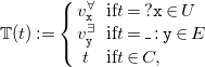\begin{align*} {\mathbb{T}}(t) := \left \{ \begin{array}{ccl} {v_{\mathtt {x}}^{\forall }} && \text{if}t=\mathtt {? x}\in U \\ {v_{\mathtt {y}}^{\exists }} && \text{if}t=\mathtt {\_:y}\in E \\ t && \text{if} t\in C, \end{array}\right . \end{align*}

where ${v_{\mathtt {x}}^{\forall }},{v_{\mathtt {y}}^{\exists }}\in {\mathbf{V}}$ and $t\in {\mathbf{C}}$ (recall that $C={\mathbf{C}}$ ). While variables in $N_3$ belong to either $E$ or $U$ , this separation is lost under function $\mathbb{T}$ . For enhancing readability of subsequent examples, the identity of variables preserves this information by using superscripts $\exists$ and $\forall$ . Function $\mathbb{T}$ naturally extends to triples $g = \mathtt {t^{1} t^{2} t^{3}}$ : ${\mathbb{T}}(g):={\textit {tr}}({\mathbb{T}}(t^{1}), {\mathbb{T}}(t^{2}), {\mathbb{T}}(t^{3}))$ . We provide the translation for every piece $f_{i}\in F$ ( $1\leq i\leq k$ ) and later collect the full translation of $F$ as the union of its translated pieces.

4.2.1 Translating atomic pieces

If $f_{i}$ is an atomic piece, $f_{i} = \mathtt {g_{1} g_{2} \ldots g_{l}}$ for some $l\geq 1$ and each $g_{j}$ ( $1\leq j\leq l$ ) is an atomic formula. The translation of $f_{i}$ is the singleton set $\mathcal{T}(f_{i})=\{ \rightarrow \exists \mathbf{z} .\ {\mathbb{T}}(g_{1})\wedge {\mathbb{T}}(g_{2})\wedge \ldots \wedge {\mathbb{T}}(g_{l}) \}$ , where $\mathbf{z}$ is the list of translated existential variables (via $\mathbb{T}$ ) from existentials occurring in $f_i$ . For example, the formula in (15) constitutes a single piece $f_(15)$ which translates to

\begin{equation*}\mathcal{T}(f_(15)) = \left \{ \rightarrow \exists {v_{\mathtt {\mathtt {y}}}^{\exists }} .\ {\textit {tr}}(\mathtt {:lucy},\mathtt {:knows},{v_{\mathtt {\mathtt {y}}}^{\exists }}) \wedge {\textit {tr}}({v_{\mathtt {\mathtt {y}}}^{\exists }},\mathtt {:likes},\mathtt {:cake}) \right \}\text .\end{equation*}

4.2.2 Translating rules

For rule-shaped pieces $f_{i} = \mathtt {\{e_1\}= \gt \{e_2\}}$ , we also obtain a single existential rule. Recall that our PNF ensures all variables in $e_{1}$ to be universals and all universal variables in $e_{2}$ to also occur in $e_{1}$ . If $e_{1} = \mathtt {g_{1}^{1} g_{1}^{2} \cdots g_{1}^{m}}$ and $e_{2} = \mathtt {g_{2}^{1} g_{2}^{2} \cdots g_{2}^{n}}$ , $\mathcal{T}(f_{i}):=\{ \forall \mathbf{x} .\ \bigwedge _{j=1}^{m} {\mathbb{T}}(g_{1}^{j}) \rightarrow \exists \mathbf{z} .\ \bigwedge _{j=1}^{n} {\mathbb{T}}(g_{2}^{j}) \}$ where $\mathbf{x}$ and $\mathbf{z}$ are the lists of translated universals and existentials, respectively. Applying $\mathcal{T}$ to the $N_3$ formula in (4), which is a piece according to Definition 3.3, we obtain

\begin{equation*}\mathcal{T}(f_(4)) = \left \{ \forall {v_{\mathtt {\mathtt {x}}}^{\forall }}.\ {\textit {tr}}({v_{\mathtt {\mathtt {x}}}^{\forall }}, \mathtt {:knows}, \mathtt {:tom}) \rightarrow \exists {v_{\mathtt {\mathtt {y}}}^{\exists }} .\ {\textit {tr}}({v_{\mathtt {\mathtt {x}}}^{\forall }}, \mathtt {:knows}, {v_{\mathtt {\mathtt {y}}}^{\exists }}) \wedge {\textit {tr}}({v_{\mathtt {\mathtt {y}}}^{\exists }}, \mathtt {:name}, \mathtt {"Tom"}) \right \}\text ,\end{equation*}

which is the same rule as given in (8) up to a renaming of (bound) variables.

4.2.3 Translating the PNF

For a set $F = \{f_{1}, f_{2}, \ldots , f_{k}\}$ of ${N_3}^\exists$ formulae in PNF, $\mathcal{T}(F)$ is the union of all translated constituents (i.e., $\mathcal{T}(F) := \bigcup _{i=1}^{k} \mathcal{T}(f_{i})$ ). Please note that $\mathcal{T}$ does not exceed a polynomial overhead in its input size.

4.3 Correctness of the translation

Let $F$ be a set of ${N_3}^\exists$ formulae in PNF. Its translation $\mathcal{T}(F)$ provides the following soundness guarantee: For every ground model ${\mathcal{I}}[M]$ of $\mathcal{T}(F)$ , there is an interpretation of $F$ that is itself a model.

Theorem 4.2. Let $F$ be a set of ${N_3}^\exists$ formulae in PNF and ${\mathcal{I}}[M]$ a ground instance. Define the canonical interpretation of ${\mathcal{I}}[M]$ by $\mathfrak{I}({\mathcal{I}}[M]) = (C, \mathfrak{a}, \mathfrak{p})$ such that

• • $\mathfrak{a}(t) := t$ for all $t\in C$ and

• • $\mathfrak{p}(p) := \{ (s,o) \mid {\textit {tr}}(s,p,o)\in {\mathcal{I}}[M] \}$ for all $p\in C$ .

${\mathcal{I}}[M]$ is a model of $\mathcal{T}(F)$ if and only if $\mathfrak{I}({\mathcal{I}}[M])$ is a model of $F$ .

Proof. By induction on the number $k$ of pieces in $F = \{ f_{1}, f_{2}, \ldots , f_{k} \}$ :

Base: For $k=1$ , $F = \{ f \}$ and $f$ is either (a) an atomic piece or (b) a rule, being the cases we need to distinguish.

1. (a) $\mathcal{T}(F)=\mathcal{T}(f)=\{ \rightarrow \exists \mathbf{z} .\ \bigwedge _{i=1}^{n} {\textit {tr}}(s_{i}, p_{i}, o_{i}) \}$ . Every model of $\mathcal{T}(F)$ satisfies its single rule, meaning that if ${\mathcal{I}}[M]$ is a model, there is a homomorphism $h^{\star }$ from $\mathcal{A} = \{ {\textit {tr}}(s_{i},p_{i},o_{i}) \mid 1\leq i\leq n \}$ to ${\mathcal{I}}[M]$ . From ${\mathcal{I}}[M]$ we get $\mathfrak{I}({\mathcal{I}}[M])=(C,\mathfrak{a},\mathfrak{p})$ with $(s_{i},o_{i})\in \mathfrak{p}(p_{i})$ for all $i\in \{ 1,\ldots ,n \}$ . We need to show that $\mathfrak{I}({\mathcal{I}}[M])$ is a model for $F$ (i.e., for $f$ ).

   If $f$ contains existentials (i.e., $\text{comp}(f)\cap E = W$ is nonempty), we need to find a substitution $\mu \;:\; W \to C$ such that $\mathfrak{I}({\mathcal{I}}[M]) \models f\mu$ . Define $\mu \;:\; W \to C$ alongside $h^{\star }$ : $\mu (\mathtt {\_:y})=h^{\star }({v_{\mathtt {y}}^{\exists }})$ for each $\mathtt {\_:y}\in W$ . For each atomic formula $g_{j} = \mathtt {s_{j} p_{j} o_{j}}$ of $f$ , we get $\mathfrak{I}({\mathcal{I}}[M]) \models g_{j}\mu$ since ${\textit {tr}}(h^{\star }(s_{j}),h^{\star }(p_{j}),h^{\star }(o_{j}))\in {\mathcal{I}}[M]$ implies $(h^{\star }(s_{j}),h^{\star }(o_{j}))\in \mathfrak{p}(h^{\star }(p_{j}))$ and, thus, $(\mathfrak{a}(s_{j}\mu ),\mathfrak{a}(o_{j}\mu ))\in \mathfrak{p}(\mathfrak{a}(p_{j}\mu ))$ . This argument holds for every atomic formula $g_{j}$ of $f$ , implying $\mathfrak{I}({\mathcal{I}}[M])\models F$ . The converse direction uses the same argumentation backwards, constructing $h^{\star }$ from $\mu$ . If $f$ does not contain any existentials, then $f$ is itself an atomic formula and the result follows as the special case $n=1$ .

2. (b) If $F = \{ f \}$ and $f= \mathtt {\{e_1\}= \gt \{e_2\}}$ , then $\mathcal{T}(F)=\{ \forall \mathbf{x} .\ \varphi \rightarrow \exists \mathbf{z} .\ \psi \}$ where $\varphi$ and $\psi$ are translated conjunctions from $e_{1}$ and $e_{2}$ .

   Let $\mathfrak{I}({\mathcal{I}}[M])$ be a model of $F$ . To show that ${\mathcal{I}}[M]$ is a model of $\mathcal{T}(F)$ , it suffices to prove, for each match $h$ of the rule, the existence of an extension $h^{\star }$ (of $h$ ), such that $h^{\star }(\psi )\subseteq {\mathcal{I}}[M]$ . Let $h$ be a match for the body of the rule and the body of the rule is a conjunction of atoms. Define $\sigma$ with $\sigma (\mathtt {? x}):= h({v_{\mathtt {x}}^{\forall }})$ for each universal variable in $e_{1}$ . $\sigma$ is a substitution such that $\mathfrak{I}({\mathcal{I}}[M])\models e_{1}\sigma$ . In order to prove this claim, let $\mathtt {s p o}$ be a triple in $e_{1}$ . Hence, ${\textit {tr}}(s, p, o)\in \varphi$ and, by the choice of $h$ , ${\textit {tr}}(h(s), h(p), h(o))\in {\mathcal{I}}[M]$ . This implies that $(h(s), h(o))\in \mathfrak{p}(h(p))$ , which also implies $(s\sigma , o\sigma )\in \mathfrak{p}(p\sigma )$ . As this argument holds for all triples in $e_{1}$ , the claim follows. Please note that, as in case (a), this reasoning can be converted to construct a match $h$ from a substitution $\sigma$ .

   Since $\mathfrak{I}({\mathcal{I}}[M])$ is a model of $f$ , there is a substitution $\mu \;:\; \text{comp}(e_{2})\cap E \to C$ , such that $\mathfrak{I}({\mathcal{I}}[M])\models e_{2}\sigma \mu$ . Define $h^{\star } := h \cup \{ w\mapsto \mu (w) \mid w\in \text{comp}(e_{2})\cap E \}$ . It holds that $h^{\star }$ satisfies match $h$ since for each atomic formula $\mathtt {s_{i} p_{i} o_{i}}$ of $e_{2}$ , we get $\mathfrak{a}(\mu (\sigma (s_{i})),\mu (\sigma (o_{i})))\in \mathfrak{p}(\mathfrak{a}(\mu (\sigma (p_{i}))))$ implying ${\textit {tr}}(\mu (\sigma (s_{i})), \mu (\sigma (p_{i}), \mu (\sigma (o_{i}))))\in {\mathcal{I}}[M]$ and $h^{\star }({\mathbb{T}}(x))=\mu (\sigma (x))$ ( $x\in \{ s_{i}, p_{i}, o_{i} \}$ ) providing a match for ${\textit {tr}}({\mathbb{T}}(s_{i}), {\mathbb{T}}(p_{i}), {\mathbb{T}}(o_{i}))$ (part of the head $\psi$ ). As this argument holds for all atomic formulae of $e_{2}$ , match $h$ is satisfied via $h^{\star }$ . As before, the construction can be inverted, obtaining $\mu$ from $h^{\star }$ and $\sigma$ from $h$ , which completes the proof for this case.

Step: Let $F = \{ f_{1}, f_{2}, \ldots , f_{k}, f_{k+1} \}$ be a set of ${N_3}^\exists$ formulae in PNF. By induction hypothesis, ${\mathcal{I}}[M]$ is a model of $\mathcal{T}(\{ f_{1}, f_{2}, \ldots , f_{k} \})$ if and only if $\mathfrak{I}({\mathcal{I}}[M])$ is a model of $\{ f_{1}, f_{2}, \cdots , f_{k} \}$ . Also by induction hypothesis, ${\mathcal{I}}[M]$ is a model of $\mathcal{T}(\{ f_{k+1} \})$ iff $\mathfrak{I}({\mathcal{I}}[M])$ is a model of $\{ f_{k+1} \}$ . Thus, ${\mathcal{I}}[M]$ is a model of $\mathcal{T}(F)$ if and only if it is a model of $\mathcal{T}(\{ f_{1} f_{2} \cdots f_{k} \})$ and of $\mathcal{T}(\{ f_{k+1} \})$ if and only if $\mathfrak{I}({\mathcal{I}}[M])$ is a model of $\{ f_{1} f_{2} \cdots f_{k} \}$ and of $\{ f_{k+1} \}$ if and only if $\mathfrak{I}({\mathcal{I}}[M])$ is a model of $F$ .

Consequently, the only (ground) models $\mathcal{T}(F)$ has are models of the original set of ${N_3}^\exists$ formulae $F$ . To complete the correctness argument, $\mathcal{T}(F)$ can have only those models relating to the ones of $F$ , which is also true by the following theorem.

Theorem 4.3. Let $\mathfrak{M}$ be an $N_3$ interpretation, then there exists an instance ${\mathcal{I}}[M]$ such that for each set $F$ of ${N_3}^\exists$ formulae in PNF

\begin{equation*}\mathfrak{M}\models F \text{ if and only if } \mathfrak{I}({\mathcal{I}}[M])\models F\end{equation*}

(cf. Theorem 4.2 ).

Proof. For $\mathfrak{M}=({\mathfrak{D}},\mathfrak{a},\mathfrak{p})$ , define $\mathfrak{M}_g=(C,\mathfrak{b},\mathfrak{q})$ such that (a) $\mathfrak{b}$ is the identity on $C$ (i.e., $\mathfrak{b}(c)=c$ for all $c \in C$ ) and (b) $\mathfrak{q}(p) := \{ (s,o) \mid (\mathfrak{a}(s),\mathfrak{a}(o))\in \mathfrak{p}(\mathfrak{a}(p)) \}$ for all $p\in C$ . Based on $\mathfrak{M}_g$ , we can define instance ${\mathcal{I}}[M] := \{ {\textit {tr}}(s,p,o) \mid (s,o)\in \mathfrak{q}(p) \}$ .

Since $\mathfrak{I}({\mathcal{I}}[M]) = \mathfrak{M}_g$ , it remains to be shown that $\mathfrak{M}\models F$ if and only if $\mathfrak{M}_g \models F$ . We proceed by induction on (the number of pieces) $|F|=k$ .

Base: If $k=1$ , then $F = \{ f \}$ and two cases arise: (a) $f$ is an atomic piece $\mathtt {g_1 \cdots g_l}$ (for some $l \geq 1$ ) and (b) $f$ is an $N_3$ rule $\mathtt {\{e_1\}= \gt \{e_2\}}$ .

1. (a) $\mathfrak{M}\models f$ if and only if $\mathfrak{M}\models f\mu$ for some $\mu \;:\; \text{comp}(f)\cap E \to C$ if and only if for each atomic formula $g_i = \mathtt {s_i p_i o_i}$ in $f$ , $(\mathfrak{a}(\mu (s_i)),\mathfrak{a}(\mu (o_i)))\in \mathfrak{p}(\mathfrak{a}(\mu (p_i)))$ (by the semantics of ${N_3}^\exists$ ) if and only if $(\mathfrak{b}(\mu (s_i)),\mathfrak{b}(\mu (o_i)))\in \mathfrak{q}(\mathfrak{b}(\mu (p_i)))$ (by construction of $\mathfrak{M}_g$ ) if and only if $\mathfrak{M}_g\models f\mu$ if and only if $\mathfrak{M}_g\models f$ (by the semantics of ${N_3}^\exists$ ).

2. (b) $\mathfrak{M}\models f$ if and only if, for each substitution $\sigma \;:\; U \to C$ with $\mathfrak{M}\models e_{1}\sigma$ , there is a substitution $\mu \;:\; \text{comp}(e_2) \cap E \to C$ such that $\mathfrak{M}\models e_{2}\sigma \mu$ .

   For respective substitutions $\sigma \;:\; U \to C$ and $\mu \;:\; \text{comp}(e_{2})\cap E \to C$ , $\mathfrak{M}\models e_{1}\sigma$ if and only if $(\mathfrak{a}(\sigma (s)),\mathfrak{a}(\sigma (o)))\in \mathfrak{p}(\mathfrak{a}(\sigma (p)))$ for each atomic formula $\mathtt {s p o}$ in $e_{1}$ (by the semantics of ${N_3}^\exists$ ) if and only if $(\mathfrak{b}(\sigma (s)),\mathfrak{b}(\sigma (o)))\in \mathfrak{q}(\mathfrak{b}(\sigma (p)))$ for each atomic formula $\mathtt {s\;p\;o}$ of $e_{1}$ if and only if $\mathfrak{M}_g\models e_{1}\sigma$ .

   The same argument can be used to argue for $\mathfrak{M}\models e_{2}\sigma \mu$ if and only if $\mathfrak{M}_g\models e_{2}\sigma \mu$ . Thus, for each $\sigma \;:\; U \to C$ for which $\mathfrak{M}\models e_{1}\sigma$ there is a substitution $\mu \;:\; \text{comp}(e_{2})\cap E \to C$ such that $\mathfrak{M}\models e_{2}\sigma \mu$ and we obtain $\mathfrak{M}_g\models e_{1}\sigma$ and $\mathfrak{M}_g\models e_{2}\sigma \mu$ , and vice versa.

Step: For $F=\{ f_{1}, \ldots , f_{k}, f_{k+1} \}$ , the induction hypothesis applies to $F'=\{ f_{1}, \ldots , f_{k} \}$ and $F'' = \{ f_{k+1} \}$ :

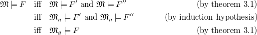\begin{align*} \mathfrak{M}\models F\quad & \text{iff}\quad \mathfrak{M}\models F' \text{ and } \mathfrak{M}\models F'' &\text{(by theorem 3.1)}\\ &\text{iff}\quad \mathfrak{M}_g\models F' \text{ and } \mathfrak{M}_g\models F'' & \text{(by induction hypothesis)}\\ & \text{iff}\quad \mathfrak{M}_g\models F & \text{ (by theorem 3.1)} \end{align*}

In the conference version of this paper, we have shown the following result to justify correctness of $\mathcal{T}$ , relating equivalent $N_3$ formulae to their translations.

Corollary 4.4 (Theorem 2 (Arndt and Mennicke 2023a)). For sets of ${N_3}^\exists$ formulae $F$ and $G$ in PNF, $F {\mathrel {\equiv }} G$ if and only if $\mathcal{T}(F) {\mathrel {\leftrightarrows }} \mathcal{T}(G)$ .

This kind of correctness argument has been coined to the term of full abstraction (Gorla and Nestmann 2016).

Proof. Let $F$ and $G$ be sets of ${N_3}^\exists$ formulae in PNF. The proof disects the statement in its two logical parts:

• Soundness ( $\Rightarrow$ ) Assume $F {\mathrel {\equiv }} G$ . We need to show that $\mathcal{T}(F) {\mathrel {\leftrightarrows }} \mathcal{T}(G)$ . Let ${\mathcal{I}}[M]$ be a ground model of $\mathcal{T}(F)$ . Then by Theorem4.2, $\mathfrak{I}({\mathcal{I}}[M])$ is a model of $F$ . By assumption ( $F {\mathrel {\equiv }} G$ ), $\mathfrak{I}({\mathcal{I}}[M])$ is a model of $G$ and, again by an application of Theorem4.2, we get that ${\mathcal{I}}[M]$ must be a model of $\mathcal{T}(G)$ . Hence, $\mathcal{T}(F) {\mathrel {\leftrightarrows }}_g \mathcal{T}(G)$ which implies $\mathcal{T}(F) {\mathrel {\leftrightarrows }} \mathcal{T}(G)$ by Lemma 4.1. The converse direction, starting from ground models of $\mathcal{T}(G)$ , uses the inverse argumentation.

• Completeness ( $\Leftarrow$ ) We prove the contrapositive: implies . Assume . Then there is a model $\mathfrak{M}$ such that $\mathfrak{M} \models F$ and , or vice versa. Since the cases are symmetric, without loss of generality, assume $\mathfrak{M} \models F$ and and suppose, towards a contradiction, that $\mathbf{(\star )}$ $\mathcal{T}(F) {\mathrel {\leftrightarrows }} \mathcal{T}(G)$ . By Theorem4.3, there is an instance ${\mathcal{I}}[M]$ such that $\mathfrak{M} \models H$ if and only if $\mathfrak{I}({\mathcal{I}}[M]) \models H$ for arbitrary sets $H$ of ${N_3}^\exists$ formulae in PNF. Thus, $\mathfrak{I}({\mathcal{I}}[M]) \models F$ and $\mathbf{(\star \star )}$ . By Theorem4.2, we get that ${\mathcal{I}}[M] \models \mathcal{T}(F)$ and, by assumption $\mathbf{(\star )}$ , ${\mathcal{I}}[M] \models \mathcal{T}(G)$ . But then Theorem4.2 allows for the conclusion that $\mathfrak{I}({\mathcal{I}}[M]) \models G$ , contradicting $\mathbf{(\star \star )}$ . Therefore, the assumption $\mathbf{(\star )}$ is false, meaning .

In the conference version of this paper, Corollary 4.4 originated from the attempt to evade trivial and/or unexpectedly simple yet undesirable transformations, which our transformation function $\mathcal{T}$ does not belong to because it possesses even stronger guarantees as proven in Theorems4.2 and 4.3. For instance, consider a translation $\mathcal{T}_0$ mapping all sets of ${N_3}^\exists$ formulae in PNF to some fixed set of rules $\Sigma _0$ (e.g., $\Sigma _0 = \emptyset$ ). This translation is surely sound since the image of $\mathcal{T}_0$ consists of the single set of rules $\Sigma _0$ , being trivially equivalent to itself. On the other hand, requiring completeness rules out $\mathcal{T}_0$ as a good transformation, since also non-equivalent $N_3$ formulae map to the same (i.e., equivalent) rule program.

While $\mathcal{T}_0$ can be ruled out as trivially incomplete by Corollary 4.4, undesirable transformations are still in reach: Consider an arbitrary enumeration of equivalence classes of sets of ${N_3}^\exists$ formulae in PNF $\mathfrak{F}_1, \mathfrak{F}_2, \mathfrak{F}_3, \ldots$ and for each of these classes a first (e.g., the lexicographically smallest) element $\mathbf{1^{st}}(\mathfrak{F}_i)$ . Define $\mathcal{T}_1(F) := \mathcal{T}(\mathbf{1^{st}}(\mathfrak{F}_{i+1}))$ if $F \in \mathfrak{F}_i$ . $\mathcal{T}_1$ is sound and complete in the sense of Corollary 4.4, but fails in having stronger guarantees on the relationship between the different semantic worlds. $\mathcal{T}_1(F)$ may end up with a rule program that speaks about a completely different vocabulary – in consequence, completely different subjects – than $F$ does. Even worse, the correctness of $\mathcal{T}_1$ does not even require the intermediate transformation $\mathcal{T}$ to be correct in any way: different equivalence classes must just be associated with (semantically) different rule programs.

$\mathcal{T}_0$ is incomplete with respect to Corollary 4.4. $\mathcal{T}_1$ on the other hand satisfies Corollary 4.4 but it does not share the same strong characteristics of $\mathcal{T}$ proven in Theorems4.2 and 4.3: Models of translated formulas cannot easily be converted into models of the original $N_3$ formula, making such transformations hard to use in contexts in which we want to employ existential rule reasoning as alternatives to existing $N_3$ reasoners. In retrospect, the connection between $N_3$ models and models of existential rules through $\mathcal{T}$ turns out to be much deeper than captured by Corollary 4.4 alone. This depth has been exploited within the proof of Corollary 4.4 that used to be available in our technical appendix (Arndt and Mennicke 2023b) only. Nevertheless, most parts of the original proofs are kept and allow for the stronger statements we now describe by Theorems4.2 and 4.3. The new and stronger formulation is meaningful to reasoning since all reasoning results can be translated back-and-forth through $\mathcal{T}$ . It is the combination of Theorems 4.2 and 4.3 and Corollary 4.4 that makes our function $\mathcal{T}$ a useful contribution. Note that similar (and further) issues regarding full abstraction have been uncovered in other communities before (Gorla and Nestmann 2016; Parrow 2016).

Apart from correctness of $\mathcal{T}$ and the close connection between $N_3$ models and models of transformed ${N_3}^\exists$ formulae, we have no further guarantees. As ${N_3}^\exists$ reasoning does not necessarily stop, there is no need for termination of the chase over translated rule programs. We expect that the similarity between the identified $N_3$ fragment of ${N_3}^\exists$ and existential rules allows for the adoption of sufficient conditions for finite models, for instance, by means of acyclicity (see Cuenca Grau et al. 2013 for a survey).

5 Reasoning with lists

So far, we discussed ${N_3}^{\exists }$ as a fragment of $N_3$ which can directly be mapped to existential rules. In this section, we detail how ${N_3}^{\exists }$ and our translation to existential rules can be extended towards supporting lists. Lists is a very important concept in $N_3$ . We first explain them in more detail and provide their semantics. Then we explain how lists and list functions can be covered by existential rules. We finish the section by discussing different ways to implement list functions in $N_3$ .

5.1 $N_3$ lists

Before introducing them formally, we explain the role of lists in Notation3 Logic by examples. $N_3$ is based on RDF, but, in contrast to RDF, N3 treats lists as first-class citizens. To illustrate this, we take a closer look at the following triple containing a list:

(16) \begin{equation} \mathtt {:lucy\;\;:likes (:cake\;\;:chocolate\;\;:tea).} \end{equation}

Stating that lucy likes cake, chocolate and tea. If we understand the above as an example of RDF-turtle (Beckett et al. 2014), the list-notation ( ) is syntactic sugar for:

(17) \begin{align} & \mathtt {:lucy\;\;:likes\;\;\_:l1. }\\ & \mathtt {\_:l1 rdf:first\;\;:cake; rdf:rest\;\;\_:l2.}\nonumber \\ &\mathtt {\_:l2 rdf:first\;\;:chocolate; rdf:rest\;\;\_l3.}\nonumber \\ &\mathtt {\_:l3 rdf:first\;\;:tea; rdf:rest rdf:nil.} \nonumber \end{align}

According to RDF semantics the predicates rdf:first and rdf:rest are properties whose domain is the class of lists, for rdf:rest the range is the class of lists and rdf:nil is itself a list. Their meaning is not specified any further.

In $N_3$ , the list in (16) itself is understood as a resource and not just as syntactic sugar for (17). The predicates rdf:first and rdf:rest have a more specific meaning: they stand for the relation between a list and its first element, a list and its rest list, that is the list, we obtain if we remove the first element, respectively. The rule

(18) \begin{equation} \mathtt {\{ \;(:a\;\;:b\;\;:c)\;\; rdf:first\;\;?x;\;\;rdf:rest\;\;?y\}= \gt \{?x\;\;:and\;\;?y\}.} \end{equation}

for example, yields

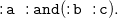(19) \begin{equation} \mathtt { :a\;\;:and (:b\;\;:c).} \end{equation}

The constant rdf:nil stands for the empty list and can also be written as ( ).

If we define the semantics in a naive way, $N_3$ ’s view of lists is not fully compatible with the (syntactic sugar) view of RDF. Suppose, we have a new triple stating the food preferences of Tom (which coincide with Lucy’s preferences):

(20) \begin{equation} \mathtt {:tom\;\;:likes\;\;(:cake\;\;:chocolate\;\;:tea).} \end{equation}

If we apply the $N_3$ rule

(21) \begin{equation} \mathtt {\{?x\;\;:likes\;\;?z.\;\;?y\;\;:likes\;\;?z\}= \gt \{?x\;\;:sharesPreferencesWith\;\;?y\}.} \end{equation}

on triple (20) and (16), we retrieve ¹⁵ that

(22) \begin{equation} \mathtt {:lucy\;\;:sharesPreferencesWith\;\;:tom.} \end{equation}

Now, we replace (20) by the first-rest combination it stands for, namely

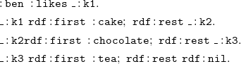(23) \begin{align} & \mathtt {:ben\;\;:likes\;\;\_:k1. } \\ & \mathtt {\_:k1\;\;rdf:first\;\;:cake;\;\;rdf:rest\;\;\_:k2.}\nonumber \\ &\mathtt {\_:k2 rdf:first\;\;:chocolate;\;\;rdf:rest\;\;\_:k3.}\nonumber \\ &\mathtt {\_:k3\;\;rdf:first\;\;:tea;\;\;rdf:rest\;\;rdf:nil.} \nonumber \end{align}

If we again apply rule (21), but this time on the list representations (17) and (23), it is not evident that we get triple (22) as a result. The lists are represented by blank nodes _:l1 and _:k1, and it is not immediately clear that these refer to the same list. The original informal $N_3$ specification overcomes the problems caused by the different representations by providing the following three axioms (Berners-Lee et al. 2008; Berners-Lee and Connolly 2011):

Existence of Lists All lists exist. That is, the triple [rdf:first :a; rdf:rest rdf:nil]. does not carry any new information.

Uniqueness of Lists Two lists having the same rdf:first-element and also the same rdf:rest-element are equal. If we add the notion of equality ¹⁶ (=): {?L1 rdf:first ?X; rdf:rest ?R. ?L12 rdf:first ?X; rdf:rest ?R.} = > {?L1 = ?L2}.

Functionality The predicates rdf:first and rdf:rest are functional properties. If we again add equality (=): {?S rdf:first ?O1, ?O2.}= > {?O1 = ?O2}. {?S rdf:rest ?O1, ?O2.}= > {?O1 = ?O2}.

The first axiom guarantees that there is no new informaion added when translating from the native list notation (16) to the first-rest noation (17). The second and the third are important for the other direction, and, in a modified version, also for the purposes of our research which is to express $N_3$ lists and list predicates by means of existential rules. We will come back to that in Subsection 5.2.

Before introducing the non-basic list predicates, we provide the syntax and semantics of the extension of ${N_3}{}^{\exists }$ with basic lists. We start with the syntax and extend the grammar provided in Figure 1 as follows:

• • the set $\mathtt {t}$ of term additionally contains the empty list () and the concept (l) of list terms, with

  \begin{align*} \mathtt {l\;\;::= }&\\ & \mathtt {t}\\ & \mathtt {l\;\;t} \end{align*}

• • the set $\mathtt {n}$ of N3 terms additionally contains the concept (k) of N3 list terms, with

  \begin{align*} \mathtt {k\;\;::= }&\\ & \mathtt {n}\\ & \mathtt {k\;\;n} \end{align*}

We further need to extend the application of a substitution introduced in Subsection 3.2 by $\mathtt {(t}_1 \ldots \mathtt {t}_n\mathtt {)}\sigma = \mathtt {(t}_1\sigma \ldots \mathtt {t}_n\sigma \mathtt {)}$ if $x= \mathtt {(t}_1 \ldots \mathtt {t}_n\mathtt {)}$ is a list, and the object function $\mathfrak{a}$ of N3 interpretations $\mathfrak{I}=(\mathfrak{D}, \mathfrak{a}, \mathfrak{p})$ as follows: If $\mathtt {t}=\mathtt {(t}_1 \ldots \mathtt {t}_n\mathtt {)}$ then $\mathfrak{a}(\mathtt {t})=(\mathfrak{a} (\mathtt {t}_1) \ldots \mathfrak{a}(\mathtt {t}_n))$ . If $\mathtt {t}=\mathtt {()}$ then $\mathfrak{a}(\mathtt {t})=()$ .

Note, that with our extension the domain $\mathfrak{D}$ of a model for a graph containing a list term also needs to contain a list of domain elements. However, the number of lists necessarily contained in $\mathfrak{D}$ is determined by the number of lists which can be produced using the alphabet. It is countable and does not depend on $\mathfrak{D}$ itself. If $\mathfrak{D}$ contains all lists which can be constructed using the interpretations of the $N_3$ terms, then axiom 1 (existence of lists) is fulfilled.

We finish the definition of the semantics of ${N_3}{}^{\exists }$ with basic lists as follows:

Given an $N_3$ alphabet which contains the list constants rdf:first and rdf:rest, and an $N_3$ Interpretation $\mathfrak{I}=(\mathfrak{D}, \mathfrak{a}, \mathfrak{p})$ . We say that $\mathfrak{I}$ is a model according to the simple list semantics of a formula $\phi$ , written as $\mathfrak{I}\models _{sl} \phi$ iff $\mathfrak{I}\models \phi$ and for triples containing rdf:first or rdf:rest in predicate position:

• • $\mathfrak{I}\models _{sl} s\ \mathtt {rdf:first}\ o.$ iff $\mathfrak{a}(s)=(s_1 \ldots s_n)$ and $\mathfrak{a}(o)=s_1$

• • $\mathfrak{I}\models _{sl} s\ \mathtt {rdf:rest}\ o.$ iff $\mathfrak{a}(s)=(s_1 \, s_2\ldots s_n)$ and $\mathfrak{a}(o)=( s_2\ldots s_n)$

Note that with this definition, we also fulfill the two missing axioms stated above. The syntactic list structure maps to a list structure in the domain of discourse. This domain list can only have one first element and only one rest list, and it is fully determined by these two parts.

In addition to rdf:first and rdf:rest, $N_3$ contains a few more special predicates which make it easier to handle lists. In our list-extension of ${N_3}{}^\exists$ we include ¹⁷ list:last, list:in, list:member, list:append, and list:remove: list:last is used to relate a list to its last argument ¹⁸ ((:a :b :c) list:last :c.), list:member defines the relation between a list and its member ( (:a :b :c) list:member :a, :b, :c.), list:in is the inverse of list:member (:b list:in (:a :b :c).), list:append expresses that the list in object position is the combination of the two lists in subject position (((:a :b) (:c :d)) list:append (:a :b :c :d).), and by list:remove we express that the object list is the list we get by removing all occurrences of the second argument of the subject list of the first argument of the subject list (((:a :b :a :c) :a) list:remove (:b :c).).

Note, that $N_3$ built-ins are not defined as functions but as relations. As a consequence of that, they can be used in different ways. We illustrate this on the predicate list:append. If we write the following rule

(24) \begin{equation} \mathtt {\{((:a\;\;:b)\;(:c\;\;:d))\;list:append\;?x\}= \gt \{:result\;\;:is\;?x\}.} \end{equation}

a reasoner will retrieve

(25) \begin{equation} \mathtt {:result\;\;:is\;(:a\;\;:b\;\;:c\;\;:d).} \end{equation}

But we can also write a rule like

(26) \begin{equation} \mathtt {\{(?x\;?y)\;list:append\;(:a\;\;:b\;\;:c)\}= \gt \{?x\;\;:and\;?y\}.} \end{equation}

which yields

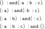\begin{align*} & \mathtt {()\;\;:and (:a\;\;:b\;\;:c).}\\ & \mathtt {(:a)\;\;:and (:b\;\;:c).}\\ & \mathtt {(:a\;\;:b)\;\;:and (\;\;:c).}\\ & \mathtt {(:a\;\;:b\;\;:c)\;\;:and\;\;().} \end{align*}

Additionally, it is possible that only one of the two variables in the subject list is instantiated, with

(27) \begin{equation} \mathtt {\{((:a\;\;:b)\;\;?y)\;\;list:append\;\;(:a\;\;:b\;\;:c)\}= \gt \{:we\;\;:get\;\;?y\}.} \end{equation}

for example, we get

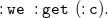(28) \begin{equation} \mathtt {:we\;\;:get\;\;(:c).} \end{equation}

On a practical level, however, this understanding of built-ins as relations comes with some limitations. If the presence of a built-in predicate causes a rule to produce infinitely many results, like it is the case with

(29) \begin{equation} \mathtt {\{?x\;\;list:last\;\;:c\}= \gt \{:we\;\;:get\;\;?x\}.} \end{equation}

where all possible lists having :c as last element need to be produced, reasoning engines normally ignore the rule. ¹⁹ We will define the full meaning of built-in predicates in our semantics, but our translation to existential rules provided in the next section will only focus on built-in predicates producing a limited number of solutions.

We now come to the semantics of list predicates. Given an $N_3$ alphabet which contains the list constants rdf:first, rdf:rest, list:in, list:member, list:append, list:last and list:remove, and an $N_3$ Interpretation $\mathfrak{I}=(\mathfrak{D}, \mathfrak{a}, \mathfrak{p})$ . We say that $\mathfrak{I}$ is a model according to list semantics of a formula $\phi$ , written as $\mathfrak{I}\models _l \phi$ iff $\mathfrak{I}\models _{sl}\phi$ and the following conditions hold:

• • $\mathfrak{I}\models _l s\ \mathtt {list:in}\ o.$ iff $\mathfrak{a}(o)=(o_1 \ldots o_n)$ and $\mathfrak{a}(s)= o_i$ for some $i$ with $1 \leq i \leq n$ ,

• • $\mathfrak{I}\models _l s\ \mathtt {list:member}\ o.$ if $\mathfrak{a}(s)=(s_1 \ldots s_n)$ and $\mathfrak{a}(o)= s_i$ for some $i$ with $1 \leq i \leq n$ ,

• • $\mathfrak{I}\models _l s\ \mathtt {list:append}\ o.$ iff $\mathfrak{a}(s)=((a_1 \ldots a_n)(b_1 \ldots b_m))$ , $0\leq n$ , $0\leq m$ , and $\mathfrak{a} (o)=(a_1 \ldots a_n \, b_1 \ldots b_m)$ ,

• • $\mathfrak{I}\models _l s\ \mathtt {list:last}\ o$ iff $\mathfrak{a}(s)=(s_1 \ldots s_n)$ and $\mathfrak{a}(o)=s_n$ ,

• • $\mathfrak{I}\models _l s\ \mathtt {list:remove}\ o$ iff $\mathfrak{a}(s)=((a_1 \ldots a_n)\, b)$ and $\mathfrak{a} (o)=(a_i)_{a_i\neq b}$

In the next section we discuss how lists and list predicates can be modeled with existential rules.

5.2 Implementing N3 lists in exitential rules

We model lists alongside the RDF representation of the previous subsection, sticking to the criteria imposed by N3, predominantly uniqueness of lists and functionality. For readability purposes we subsequently diverge from using our triple predicate $\textit {tr}$ for predicates concerning lists. Instead of ${\textit {tr}}(x, \mathtt {rdf:first}, y)$ we use an auxiliary binary predicate $\textit {first}$ and write $\textit {first}(x,y)$ . Similarly we use $\textit {rest}(x,y)$ to denote ${\textit {tr}}(x,\mathtt {rdf:rest}, y)$ . For technical reasons, we use a unary predicate $\textit {list}$ to identify all those objects that are lists. Before modeling lists and their functions, let us formulate the criteria based on the three predicates: A model ${\mathcal{I}}[M]$ of rule set $\Sigma$ and database ${\mathcal{D}}$ satisfies

Uniqueness of Lists if for all lists $l_1$ and $l_2$ (i.e., $\textit {list}(l_1), \textit {list}(l_2) \in {\mathcal{I}}[M]$ ), $\textit {first}(l_1, x), \textit {first}(l_2, x)\in {\mathcal{I}}[M]$ and $\textit {rest}(l_1, r), \textit {rest}(l_2, r) \in {\mathcal{I}}[M]$ implies $l_1 = l_2$ ;

Functionality if for all lists $l$ (i.e., $\textit {list}(l) \in {\mathcal{I}}[M]$ ), $\textit {first}(l, x), \textit {first}(l, y) \in {\mathcal{I}}[M]$ implies $x=y$ , and $\textit {rest}(l, x), \textit {rest}(l, y)\in {\mathcal{I}}[M]$ implies $x=y$ .

Towards Existence of Lists, we ensure existence of the empty list:

(30) \begin{eqnarray} & \rightarrow & \textit {list}(\mathtt {rdf:nil}) \end{eqnarray}

Given that many rule reasoners operate via materialization of derived facts, we should not fully implement the Existence of Lists criterion since materializing all lists certainly entails an infinite process. Instead, we create lists on-demand. The binary getList predicate expects a list element $x$ (to be added) and a list $l$ , and creates a new list with first element $x$ and rest $l$ :

(31) \begin{eqnarray} \textit {getList}(x, l) \wedge \textit {list}(l) & \rightarrow & \exists l' .\ \textit {list}(l') \wedge \textit {first}(l', x) \wedge \textit {rest}(l', l) \end{eqnarray}

With this interface in place, we replicate example (16) as follows:

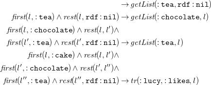\begin{align*} & \rightarrow \textit {getList}(\mathtt {:tea}, \mathtt {rdf:nil}) \\ \textit {first}(l, \mathtt {:tea}) \wedge \textit {rest}(l, \mathtt {rdf:nil}) & \rightarrow \textit {getList}(\mathtt {:chocolate}, l) \\ \textit {first}(l, \mathtt {:chocolate}) \wedge \textit {rest}(l, l') \wedge \\ \textit {first}(l', \mathtt {:tea}) \wedge \textit {rest}(l', \mathtt {rdf:nil}) & \rightarrow \textit {getList}(\mathtt {:tea}, l) \\ \textit {first}(l, \mathtt {:cake}) \wedge \textit {rest}(l, l') \wedge \\ \textit {first}(l', \mathtt {:chocolate}) \wedge \textit {rest}(l', l'') \wedge \\ \textit {first}(l'', \mathtt {:tea}) \wedge \textit {rest}(l'', \mathtt {rdf:nil})& \rightarrow {\textit {tr}}(\mathtt {:lucy}, \mathtt {:likes}, l) \end{align*}

This rather cumbersome encoding implements Uniqueness of Lists. Towards a much simpler encoding, suppose we only take the following rule obtaining the same list as above:

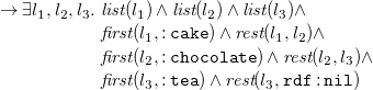(32) \begin{equation} \begin{array}{rcl} & \rightarrow \exists l_1, l_2, l_3 . & \textit {list}(l_1) \wedge \textit {list}(l_2) \wedge \textit {list}(l_3) \wedge \\ && \textit {first}(l_1, \mathtt {:cake}) \wedge \textit {rest}(l_1, l_2) \wedge \\ && \textit {first}(l_2, \mathtt {:chocolate}) \wedge \textit {rest}(l_2, l_3) \wedge \\ && \textit {first}(l_3, \mathtt {:tea}) \wedge \textit {rest}(l_3, \mathtt {rdf:nil}) \end{array} \end{equation}

The rule itself can now be combined with other rules as well as the previous one. However, uniqueness can be violated when the restricted chase is used for reasoning. Recall from Subsection 4.1 that the restricted chase creates new facts (by instantiating rule heads) only if the rule matches are not yet satisfied. Suppose we create an alternative list that is the same as before but replaces :cake for :cookies:

(33) \begin{equation} \begin{array}{rcl} & \rightarrow \exists l_1, l_2, l_3 . & \textit {list}(l_1) \wedge \textit {list}(l_2) \wedge \textit {list}(l_3) \wedge \\ && \textit {first}(l_1, \mathtt {:cookies}) \wedge \textit {rest}(l_1, l_2) \wedge \\ && \textit {first}(l_2, \mathtt {:chocolate}) \wedge \textit {rest}(l_2, l_3) \wedge \\ && \textit {first}(l_3, \mathtt {:tea}) \wedge \textit {rest}(l_3, \mathtt {rdf:nil}) \end{array} \end{equation}

While the list created by rule (33) is surely distinct from the one created through rule application of (32), they also obtain different sublists. After a restricted chase over rule set {(32), (33) } and the empty database, we get two distinct lists $l$ and $l'$ such that $\textit {first}(l, \mathtt {:tea})$ , $\textit {first}(l', \mathtt {:tea}), \textit {rest}(l,\mathtt {rdf:nil}), \textit {rest}(l',\mathtt {rdf:nil})$ , contradicting Uniqueness of Lists. The reason for this is that the application condition of the restricted chase checks whether the head of the rule is already satisfied. If not, the full head is instantiated with (globally) fresh nulls in place of the existentially quantified variables. Our encoding via rule (31) overcomes this issue by step-wise introducing new list elements. If a sublist already exists, rule creation is not triggered redundantly.

Theorem 5.1. Let ${\mathcal{D}}$ be a database, $\Sigma$ a rule set, and $\mathcal{I}$ the restricted chase of $\Sigma$ and ${\mathcal{D}}$ . If the only rules in $\Sigma$ using predicates list, first, or rest in their heads are those of (30) and (31), then $\mathcal{I}$ satisfies (a) Uniqueness of Lists and (b) Functionality .

Proof. Functionality follows from the fact that the only rule introducing first- and rest-atoms is (31) and, thereby, uniquely determines first and rest elements for a list term. Thus, predicates first and rest are functional.

Regarding Uniqueness of Lists, we observe that only rule (31) introduces lists together with their (functional) first and rest atoms. Hence, if there were two lists $l_1$ and $l_2$ with the same first and rest elements, then the respective chase sequence ${\mathcal{D}}^0 {\mathcal{D}}^1 {\mathcal{D}}^2 \ldots$ contains a member $\mathcal{D}^i$ in which (without loss of generality) $l_1$ is contained. Furthermore, there is a later instance ${\mathcal{D}}^j$ ( $j \gt i$ ) in which $l_2$ is not yet contained but is about to be added to ${\mathcal{D}}^{j+1}$ . But rule (31) is already satisfied in ${\mathcal{D}}^j$ for the respective first/rest elements. Thus, $l_2$ will never be instantiated by the restricted chase and can, thus, not be part of the chase.

Before we get into the intricates of appending two or more lists, let us briefly show the rules for implementing list:last and list:in (and list:member as the inverse of list:in), represented by binary predicate symbols last and isIn.

(34) \begin{eqnarray} \textit {first}(l, x) \wedge \textit {rest}(l, \mathtt {rdf:nil}) & \rightarrow & \textit {last}(x, l) \end{eqnarray}

(35) \begin{eqnarray} \textit {rest}(l, l') \wedge \textit {last}(y, l') & \rightarrow & \textit {last}(y, l) \end{eqnarray}

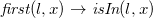(36) \begin{eqnarray} \textit {first}(l, x) & \rightarrow & \textit {isIn}(l, x) \end{eqnarray}

(37) \begin{eqnarray} \textit {rest}(l, l') \wedge \textit {isIn}(l', y) & \rightarrow & \textit {isIn}(l, y) \end{eqnarray}

Note, these rules are sufficient for creating all necessary facts to obtain the required results. Regarding list concatenation via list:append, we introduce the ternary predicate append with the appended list in the first position and the two constituent lists in second and last. First, every list $l$ prepended by the empty list yields itself:

(38) \begin{eqnarray} \textit {list}(l) \rightarrow \textit {append}(l, \mathtt {rdf:nil}, l) \end{eqnarray}

Second, if we append lists $l_1$ and $l_2$ to get $l_3$ (i.e., $\textit {append}(l_3, l_1, l_2)$ ), and $x$ is the first element of $l_2$ , then $l_3$ can also be obtained by appending $x$ to $l_1$ , and the result to the rest of $l_2$ . Therefore, we need an auxiliary set of rules that appends a single element $x$ to a list $l$ :

(39) \begin{eqnarray} \textit {append}(l_3, l_1, l_2) \wedge \textit {first}(l_2, x) & \rightarrow & \textit {getAppendS}(l_1, x) \end{eqnarray}

(40) \begin{eqnarray} \textit {getAppendS}(l, x) \wedge \textit {rest}(l, l') & \rightarrow & \textit {getAppendS}(l', x) \end{eqnarray}

Rule (39) requests a new list that starts with the same elements as $l_1$ and appends the additional element $x$ . Rule (40) recursively pushes the request through the list. Once, the empty list (rdf:nil) is reached, appending the element $x$ is the same as prepending it to rdf:nil:

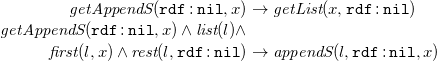(41) \begin{equation} \begin{array}{rcl} \textit {getAppendS}(\mathtt {rdf:nil}, x) & \rightarrow & \textit {getList}(x, \mathtt {rdf:nil}) \\ \textit {getAppendS}(\mathtt {rdf:nil}, x) \wedge \textit {list}(l) \wedge \\ \textit {first}(l, x) \wedge \textit {rest}(l, \mathtt {rdf:nil}) & \rightarrow & \textit {appendS}(l, \mathtt {rdf:nil}, x) \\ \end{array} \end{equation}

These rules create a fresh list with first element $x$ and rest rdf:nil if necessary. Predicate appendS stands for append singleton and, therefore, $\textit {appendS}(l, l', x)$ tells that list $l$ is the result of appending $x$ to list $l'$ . The recursive step is implemented as follows:

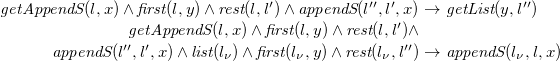(42) \begin{equation} \begin{array}{rcl} \textit {getAppendS}(l, x) \wedge \textit {first}(l, y) \wedge \textit {rest}(l, l') \wedge \textit {appendS}(l'', l', x) & \rightarrow & \textit {getList}(y, l'') \\ \textit {getAppendS}(l, x) \wedge \textit {first}(l, y) \wedge \textit {rest}(l, l') \wedge \\ \textit {appendS}(l'', l', x) \wedge \textit {list}(l_{\nu }) \wedge \textit {first}(l_{\nu }, y) \wedge \textit {rest}(l_{\nu }, l'') & \rightarrow & \textit {appendS}(l_{\nu }, l, x) \end{array} \end{equation}

So if a list $l$ shall be appended by singleton $x$ and we already know that for the rest of $l$ (i.e., $l'$ ) there is a version with appended $x$ (i.e., $l''$ ), then $l$ appended by $x$ is the new list formed by the first element of $l$ (i.e., $y$ ) and $l''$ as rest.

Last, appending two lists can also be requested via rules. Once more, we use a predicate for this request, namely getAppend. This predicate is an interface for users (i.e., other rules) to create lists beyond predicate getList. Such requests are served by the following rules:

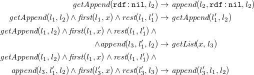\begin{eqnarray*} \textit {getAppend}(\mathtt {rdf:nil}, l_2) & \rightarrow & \textit {append}(l_2, \mathtt {rdf:nil}, l_2) \\ \textit {getAppend}(l_1, l_2) \wedge \textit {first}(l_1, x) \wedge \textit {rest}(l_1, l_1') & \rightarrow & \textit {getAppend}(l_1', l_2) \\ \textit {getAppend}(l_1, l_2) \wedge \textit {first}(l_1, x) \wedge \textit {rest}(l_1, l_1') \wedge \\ \wedge \textit {append}(l_3,l_1', l_2) & \rightarrow & \textit {getList}(x, l_3) \\ \textit {getAppend}(l_1, l_2) \wedge \textit {first}(l_1, x) \wedge \textit {rest}(l_1, l_1') \wedge \\ \textit {append}(l_3,l_1', l_2) \wedge \textit {first}(l_3', x) \wedge \textit {rest}(l_3', l_3) & \rightarrow & \textit {append}(l_3', l_1, l_2) \end{eqnarray*}

The remove functionality can be implemented in a similar fashion. Note that none of the additionally instantiated rules for list built-ins use predicates list, first, or rest in their heads. Thus, Theorem5.1 still holds in rule sets using built-in functions. Throughout the rest of this subsection we aim at showing how the framework implements the examples given throughout Subsection 5.1 as well as an example of list usage inside $N_3$ rules.

5.2.1 Appending lists

First, recall the following $N_3$ rule (cf. (24)):

\begin{equation*} \mathtt {\{((:a\;\;:b) (:c\;\;:d)) list:append ?x\}= \gt \{:result\;\;:is\;\;?x\}.} \end{equation*}

For the implementation of this rule, we need to make sure the constant lists (the operands of list:append) exist:

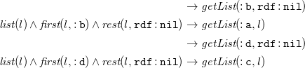\begin{eqnarray*} & \rightarrow & \textit {getList}(\mathtt {:b}, \mathtt {rdf:nil}) \\ \textit {list}(l) \wedge \textit {first}(l, \mathtt {:b}) \wedge \textit {rest}(l, \mathtt {rdf:nil}) & \rightarrow & \textit {getList}(\mathtt {:a}, l) \\ & \rightarrow & \textit {getList}(\mathtt {:d}, \mathtt {rdf:nil}) \\ \textit {list}(l) \wedge \textit {first}(l, \mathtt {:d}) \wedge \textit {rest}(l, \mathtt {rdf:nil}) & \rightarrow & \textit {getList}(\mathtt {:c}, l) \end{eqnarray*}

After these rules have been used, the lists in example (24) are guaranteed to exist. Next, we can request to append the two lists matched within the rule:

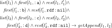\begin{eqnarray*} \textit {list}(l_1) \wedge \textit {first}(l_1, \mathtt {:a}) \wedge \textit {rest}(l_1, l_1') \wedge && \\ \textit {first}(l_1', \mathtt {:b}) \wedge \textit {rest}(l_1', \mathtt {rdf:nil}) \wedge && \\ \textit {list}(l_2) \wedge \textit {first}(l_2, \mathtt {:c}) \wedge \textit {rest}(l_2, l_2') \wedge && \\ \textit {first}(l_2',\mathtt {:d}) \wedge \textit {rest}(l_2', \mathtt {rdf:nil}) & \rightarrow & \textit {getAppend}(l_1, l_2) \end{eqnarray*}

After this rule we are guaranteed to have all lists in place for implementing our rule.

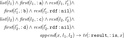\begin{eqnarray*} \textit {list}(l_1) \wedge \textit {first}(l_1, \mathtt {:a}) \wedge \textit {rest}(l_1, l_1') \wedge && \\ \textit {first}(l_1', \mathtt {:b}) \wedge \textit {rest}(l_1', \mathtt {rdf:nil}) \wedge && \\ \textit {list}(l_2) \wedge \textit {first}(l_2, \mathtt {:c}) \wedge \textit {rest}(l_2, l_2') \wedge && \\ \textit {first}(l_2',\mathtt {:d}) \wedge \textit {rest}(l_2', \mathtt {rdf:nil}) \wedge && \\ \textit {append}(x, l_1, l_2) & \rightarrow & {\textit {tr}}(\mathtt {:result}, \mathtt {:is}, x) \end{eqnarray*}

Second, we reconsider rule (26):

\begin{equation*} \mathtt {\{(?x\;\;?y) list:append (:a\;\;:b\;\;:c)\}= \gt \{?x\;\;:and\;\;?y\}.} \end{equation*}

In this example we need to ensure the resulting list exists. Our rule framework (especially rules (38)–(42)) takes care of disecting the list into its fragment. Thus, the example rule can be implemented, once the list (:a :b :c) has been created as before, by

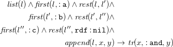\begin{eqnarray*} \textit {list}(l) \wedge \textit {first}(l, \mathtt {:a}) \wedge \textit {rest}(l, l') \wedge && \\ \textit {first}(l', \mathtt {:b}) \wedge \textit {rest}(l', l'') \wedge && \\ \textit {first}(l'', \mathtt {:c}) \wedge \textit {rest}(l'', \mathtt {rdf:nil}) \wedge && \\ \textit {append}(l, x, y) & \rightarrow & {\textit {tr}}(x, \mathtt {:and}, y) \end{eqnarray*}

5.2.2 List creation in rules

Last, we consider an $N_3$ rule that identifies two lists in its body and creates a new list based on some elements identified within the list. The following rule identifies two lists, one with three elements (?x, ?y, and ?z) and one with two elements (?a and ?b), and then creates a new list with first element ?y and a rest list with the singleton element ?b:

(43) \begin{equation} \mathtt {\{:s\;\;:p\;\;(?x\;\;?y\;\;?z).\;\;:k\;\;:l\;\;(?a\;\;?b)\}= \gt \{:h\;\;:i\;\;(?y\;\;?b)\}.} \end{equation}

This rule needs splitting into creating the list for the result and then creating the output triple:

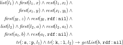\begin{eqnarray*} \textit {list}(l_1) \wedge \textit {first}(l_1, x) \wedge \textit {rest}(l_1, x_l) \wedge \\ \textit {first}(x_l, y) \wedge \textit {rest}(x_l, y_l) \wedge \\ \textit {first}(y_l, z) \wedge \textit {rest}(y_l, \mathtt {rdf:nil}) \wedge \\ \textit {list}(l_2) \wedge \textit {first}(l_2, a) \wedge \textit {rest}(l_2, a_l) \wedge \\ \textit {first}(a_l, b) \wedge \textit {rest}(a_l, \mathtt {rdf:nil}) \wedge \\ {\textit {tr}}(\mathtt {:s}, \mathtt {:p}, l_1) \wedge {\textit {tr}}(\mathtt {:k}, \mathtt {:l}, l_2) & \rightarrow & \textit {getList}(b, \mathtt {rdf:nil}) \\ \end{eqnarray*}

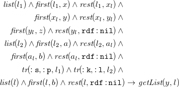\begin{eqnarray*} \textit {list}(l_1) \wedge \textit {first}(l_1, x) \wedge \textit {rest}(l_1, x_l) \wedge \\ \textit {first}(x_l, y) \wedge \textit {rest}(x_l, y_l) \wedge \\ \textit {first}(y_l, z) \wedge \textit {rest}(y_l, \mathtt {rdf:nil}) \wedge \\ \textit {list}(l_2) \wedge \textit {first}(l_2, a) \wedge \textit {rest}(l_2, a_l) \wedge \\ \textit {first}(a_l, b) \wedge \textit {rest}(a_l, \mathtt {rdf:nil}) \wedge \\ {\textit {tr}}(\mathtt {:s}, \mathtt {:p}, l_1) \wedge {\textit {tr}}(\mathtt {:k}, \mathtt {:l}, l_2) \wedge \\ \textit {list}(l) \wedge \textit {first}(l, b) \wedge \textit {rest}(l, \mathtt {rdf:nil}) & \rightarrow & \textit {getList}(y, l) \\ \end{eqnarray*}

\begin{eqnarray*} \textit {list}(l_1) \wedge \textit {first}(l_1, x) \wedge \textit {rest}(l_1, x_l) \wedge \\ \textit {first}(x_l, y) \wedge \textit {rest}(x_l, y_l) \wedge \\ \textit {first}(y_l, z) \wedge \textit {rest}(y_l, \mathtt {rdf:nil}) \wedge \\ \textit {list}(l_2) \wedge \textit {first}(l_2, a) \wedge \textit {rest}(l_2, a_l) \wedge \\ \textit {first}(a_l, b) \wedge \textit {rest}(a_l, \mathtt {rdf:nil}) \wedge \\ {\textit {tr}}(\mathtt {:s}, \mathtt {:p}, l_1) \wedge {\textit {tr}}(\mathtt {:k}, \mathtt {:l}, l_2) \wedge \\ \textit {list}(l') \wedge \textit {first}(l', b) \wedge \textit {rest}(l', \mathtt {rdf:nil}) \wedge \\ \textit {list}(l) \wedge \textit {first}(l, y) \wedge \textit {rest}(l, l') & \rightarrow & {\textit {tr}}(\mathtt {:h}, \mathtt {:i}, l) \end{eqnarray*}

This construction may become complicated if several list built-ins are co-dependent.

5.3 $N_3$ list predicates as syntactic sugar

As detailed in the previous section, $N_3$ list predicates can be expressed by means of existential rules if the reasoning is performed under similar premises as the restricted chase. This is particularly interesting in the context of Notation3 Logic: it is well-known that list predicates list:in, list:member, list:append, list:last, and list:remove introduced in Subsection 5.1 are syntactic sugar, and, therefore, can be expressed using rules in combination with the predicates rdf:first and rdf:rest. Typically these rules are only written for reasoners supporting backward-chaining, that is, with algorithms performing reasoning starting from the goal and following rules from head to body until some factual evidence is found. ²⁰

For better illustration, consider the following $N_3$ rules implementing list:append: ²¹

(44) \begin{align} \mathtt {\{(()\;\;?x)\;\;list:append\;\;?x\}\lt =}& \mathtt {\{ \}. } \end{align}

(45) \begin{align} \mathtt {\{(?x\;\;?y)\;\;list:append\;\;?z\}\lt =}& \mathtt {\{?x\;\;rdf:first\;\;?a.\;\;?x\;\;rdf:rest\;\;?r.}\\ &\mathtt { ?z\;\;rdf:first\;\;?a.\;\;?z\;\;rdf:rest\;\;?q. }\notag \\ &\mathtt { (?r\;\;?y)\;\;list:append\;\;?q\;\;\} }.\end{align}

If these rules are used in backward-chaining, they get triggered by each execution of a rule containing a triple with the predicate list:append. If we, for example, would like to get all instances of the triple :result :is ?x. which can be derived by rule (24), the triple in the body of the rule triggers rule (45), to test whether there is evidence for the triple ((:a :b) (:c :d)) list:append ?x. The rule is again followed in a backwards direction yielding:

(46) \begin{align} & \mathtt { (:a\;\;:b) rdf:first\;\;:a;\;\;rdf:rest\;\;(:b).}\\ &\mathtt { ?x\;\;rdf:first\;\;:a;\;\;rdf:rest\;\;?q. }\nonumber \\ &\mathtt { ((:b)\;\;(:c\;\;:d))\;\;list:append\;\;?q. }.\nonumber \end{align}

The triples in the first line of this example got instantiated according to the semantics of rdf:first and rdf:rest. This istantiation also caused the triples in the following two lines to partially instantiated. Since there is not enough information to instantiate the triples from the second line, a (backward) reasoner would continue with the last triple which again has list:append in predicate position. Rule (45) is called again. This time we retrieve:

(47) \begin{align} & \mathtt { (:b)\;\;rdf:first\;\;:b;\;\;rdf:rest\;\;().}\\ &\mathtt { ?q\;\;rdf:first\;\;:b;\;\;rdf:rest\;\;?q2. } \nonumber \\ &\mathtt { (() (:c\;\;:d)) list:append ?q2. }.\nonumber \end{align}

Again following the rules backwards, we can apply rule (44) to get a value for ?q2:

\begin{equation*} \mathtt { (()\;\;(:c\;\;:d))\;\;list:append (:c\;\;:d). } \end{equation*}

With this information, we get a binding for ?q in (47):

\begin{align*} & \mathtt { (:b)\;\;rdf:first\;\;:b;\;\;rdf:rest\;\;().}\\ &\mathtt { (:b\;\;:c\;\;:d)\;\;rdf:first\;\;:b;\;\;rdf:rest\;\;(:c\;\;:d). } \\ & \mathtt { (()\;(:c\;\;:d))\;list:append\;(:c\;\;:d). }. \end{align*}

Subsequently, we obtain a new binding ?x in (46):

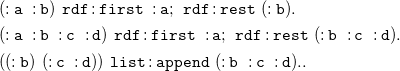\begin{align*} & \mathtt { (:a\;\;:b)\;\;rdf:first\;\;:a;\;\;rdf:rest\;\;(:b).}\\ &\mathtt { (:a\;\;:b\;\;:c\;\;:d)\;\;rdf:first\;\;:a;\;\;rdf:rest\;\;(:b\;\;:c\;\;:d ). } \\ &\mathtt { ((:b)\;\;(:c\;\;:d))\;\;list:append\;\;(:b\;\;:c\;\;:d). }. \end{align*}

This produces :we :get (:a :b :c :d). as a solution. The backward-chaining process produces triples on-demand: only if a rule premise depends on the information, a backward rule is called to retrieve it, and this allows us to have infinitely large models which we do not materialize during reasoning.

In the $N_3$ community, this and other examples are normally used to argue that $N_3$ reasoners should support backwards-reasoning as a way to only produce triples when these are needed to find instances for a goal. Following the findings of the previous subsection, it is not true that we necessarily need backward rules to support triple production on-demand. Instead of writing rule (44) and (45), we can also add the triple (:a :b) :getAppend (:c :d). to our initial rule (24). With the following rules, we retrieve the same result as above:

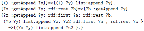
These rules follow the structure of the rules in the previous subsection with the exception that we do not need list constructors in $N_3$ . If we apply our rules to the fact above, we sucessively construct the triples (() (:c :d)) list:append (:c :d)., ((:b) (:c :d)) list:append (:b :c :d)., and ((:a :b) (:c :d)) list:append (:a :b :c :d).. These can then directly be used in rules. In more complicated cases, where the arguments of the predicate list:append do not appear partially instantiated in rule bodies, the relevant instances of the fact ?x :getAppend ?y. need to be constructed via rules just as it is the case for existential rules. As $N_3$ follows the axioms introduced in Subsection 5.1, the first-rest interpretation of RDF lists is equivalent to $N_3$ ’s representation of lists as first-class citizens. As a consequence, the rules actually work for all examples introduced above. Similarly, the other list predicates can be written by means of rdf:first and rdf:rest, and handled via backward-chaining or, alternatively, with some version of the chase.

Note, the backward rules handling list:append can be mimicked by splitting them in several forward rules acting on a getter triple, that is, a triple causing the production of the required instance of the predicate. We additionally need rules producing the required instances of that getter triple, at which point we need to be careful considering dependencies between triples. However, the mechanism introduced in the previous subsection provides us with a possibility to do reasoning on-demand in a purely forward manner.

6 Evaluation

The considerations provided above allow us to use existential rule reasoners to perform ${N_3}{}^\exists$ reasoning. We would like to find out whether our finding is of practical relevance, that is whether we can identify datasets on which existential rule reasoners, running on the rule translations, outperform classical $N_3$ reasoners provided with the original data.

In order to do this we have implemented $\mathcal{T}$ as a python script that takes an arbitrary ${N_3}^\exists$ formula $f$ , constructs its set representation $F$ in PNF, and produces the set of rules $\mathcal{T}(F)$ . This script and some additional scripts to translate existential rules (with at most binary predicates) to ${N_3}^\exists$ formulae are available on GitHub. Our implementation allows us to compare $N_3$ reasoners with existential rule reasoners, performance-wise. As existential rule reasoners we chose VLog (Carral et al. 2019), a state-of-the-art reasoning engine designed for working with large piles of input data, and Nemo (Ivliev et al. 2023), a recently released rust-based reasoning engine. As $N_3$ reasoners we chose cwm (Berners-Lee 2009) and EYE (Verborgh and De Roo 2015) which – due to their good coverage of $N_3$ features – are most commonly used. All experiments have been performed on a laptop with 11th Gen Intel Core i7-1165G7 CPU, 32 GB of RAM, and 1TB disk capacity, running a Ubuntu 22.04 LTS.

6.1 Datasets

We performed our experiments on two datasets: Lubm from the Chasebench (Benedikt et al. 2017) provides a fixed set of 136 rules and varies in the number of facts these rules are applied; the Deep Taxonomy (DT) benchmark developed for the WellnessRules project (Boley et al. 2009) consists of one single fact and a varying number of mutually dependent rules.

The Chasebench is a benchmarking suite for existential rule reasoning. Among the different scenaria in Chasebench we picked Lubm for its direct compatibility with $N_3$ : all predicates in Lubm have at most arity $2$ . Furthermore, Lubm allows for a glimpse on scalability since Lubm comes in different database sizes. We have worked with Lubm 001, 010, and 100, roughly referring to dataset sizes of a hundred thousand, one million and ten million facts. We translated Lubm data and rules into a canonical $N_3$ format. Predicate names and constants within the dataset become IRIs using the example prefix. An atom like $\textit {src_advisor}(\textit {Student441},\textit {Professor8})$ becomes the triple $\mathtt {:Student441\;\;:src\_advisor\;\;:Professor8.}$ . For atoms using unary predicates, like $\textit {TeachingAssistent}(\textit {Student498})$ , we treat $\mathtt {:TeachingAssistent}$ as a class and relate $\mathtt {:Student498}$ via $\mathtt {rdf:type}$ to the class. For any atom $A$ , we denote its canonical translation into triple format by $t(A)$ . Note this canonical translation only applies to atoms of unary and binary predicates. For the existential rule

\begin{equation*}\forall \mathbf{x} .\ B_{1} \wedge \ldots \wedge B_{m} \rightarrow \exists \mathbf{z} .\ H_{1} \wedge \ldots \wedge H_{n}\end{equation*}

we obtain the canonical translation by applying $t$ to all atoms, respecting universally and existentially quantified variables (i.e., universally quantified variables are translated to universal $N_3$ variables and existentially quantified variables become blank nodes):

\begin{equation*}\mathtt {\{} t(B_{1})\mathtt {.} \cdots t(B_{m})\mathtt {.} \mathtt {\}}\mathtt {= \gt }\mathtt {\{} t(H_{1})\mathtt {.} \cdots t(H_{n})\mathtt {.} \mathtt {\}}\text .\end{equation*}

All $N_3$ reasoners have reasoned over the canonical translation of data and rules which was necessary because of the lack of an $N_3$ version of Lubm. Since we are evaluating VLog’s and Nemo’s performance on our translation $\mathcal{T}$ , we converted the translated Lubm by $\mathcal{T}$ back to existential rules before reasoning. Thereby, former unary and binary atoms were turned into triples and then uniformly translated to $\textit {tr}$ -atoms via $\mathcal{T}$ .

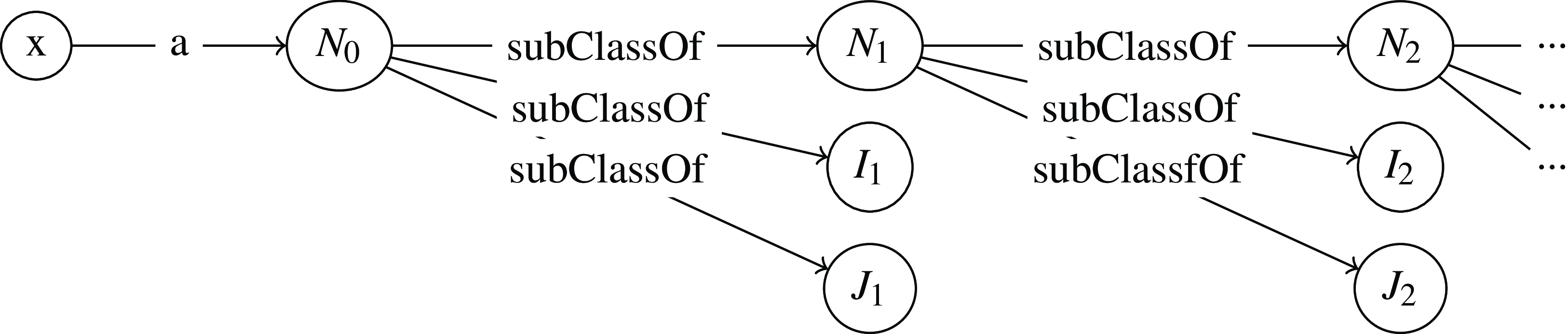
Fig. 2. Structure of the deep taxonomy benchmark.

The Deep Taxonomy benchmark simulates deeply nested RDFS-subclass reasoning. ²² It contains one individual which is member of a class. This class is subclass of three other classes of which one again is subclass of three more classes and so on. Figure 2 illustrates this idea. The benchmark provides different depths for the subclass chain and we tested with the depths of 1,000 and 100,000. The reasoning tests for the membership of the individual in the last class of the chain. For our tests, the subclass declarations were translated to rules, the triple $\mathtt {:N0\;\;rdfs:subClassOf\;\;:N1.}$ became

{ ?x a :N0.}= > { ?x a :N1.}.

This translation also illustrates why this rather simple reasoning case is interesting: we have a use case in which we depend on long chains of rules executed after each other. The reasoner EYE allows the user to decide per rule whether it is applied using forward- or backward-reasoning, at least if the head of the rule does not contain blank nodes. For this dataset, we evaluated full backward- and full forward-reasoning, separately.

6.2 Results

Table 1 presents the running times of the four reasoners and additionally gives statistics about the sizes of the given knowledge base (# facts) and the rule set (# rules). For DT we display two reasoning times for EYE, one produced by only forward reasoning (EYE-fw), one for only backward-reasoning (EYE-bw). Note, that for the latter, the reasoner does not produce the full deductive closure of the dataset, but answers a query instead. As Lubm contains rules with blank nodes in their haeds, full backward reasoning was not possible in that case, the table is left blank. EYE performs much better than VLog and Nemo for the experiments with DT. Its reasoning time is off by one order of magnitude. Conversely, VLog and Nemo could reason over all the Lubm datasets while EYE has thrown an exception after having read the input facts. The reasoning times of VLog are additionally significantly lower than the times for EYE. While Nemo shows a similar runtime on DT as VLog, it is slower on Lubm. However, we may be quite optimistic regarding its progress in runtime behavior, as Nemo already shows better running times on the original Lubm datasets. The reasoner cwm is consistently slower than the other three and from Lubm 010 on. All reasoners tried to find the query answers/deductive closures for at least ten minutes (i.e., — in Table 1 indicates a time-out).

Table 1. Experimental results

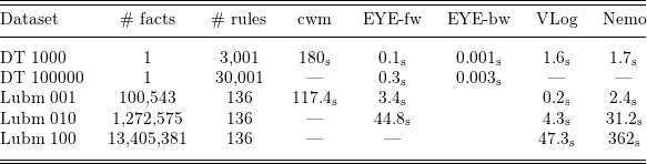
6.3 Discussion

In all our tests we observe a very poor performance of cwm which is not surprising, given that this reasoner has not been updated for some time. The results for EYE, VLog and Nemo are more interesting as they illustrate the different strengths of the reasoners.

For very high numbers of rules compared to the amount of data, EYE performs much better than VLog and Nemo. The good results of 0.1 and 0.3 s can even be improved by using backward reasoning. This makes EYE very well-suited for use cases where we need to apply complex rules on datasets of low or medium size. This could be interesting in decentralized set-ups such as policy-based access control for the Solidproject. ²³ On the other hand we see that VLog and Nemo perform best when provided with large datasets and lower numbers of rules. This could be useful use cases involving bigger datasets in the Web like Wikidata or DBpedia. ²⁴

From the perspective of this paper, these two findings together show the relevance of our work: we observed big differences between the tools’ reasoning times and these differences depended on the use cases. In other words, there are use cases which could benefit from our translation and we thus do not only make the first steps towards having more $N_3$ reasoners available but also broaden the scope of possible $N_3$ applications.

7 Related work

When originally proposed as a W3C member submission (Berners-Lee and Connolly 2011), the formal semantics of $N_3$ was only introduced informally. As a consequence, different systems, using $N_3$ , interpreted concepts like nested formulae differently (Arndt et al. 2019). Since then, the relation of $N_3$ to other Web standards has been studied from a use-case perspective (Arndt 2019) and a W3C Community group has been formed (Woensel et al. 2023), which recently published the semantics of $N_3$ without functions (Arndt and Champin 2023). Even with these definitions, the semantic relation of the logic to other standards, especially outside the Semantics Web, has not been studied thoroughly.

For $N_3$ ’s subset RDF, (De bruijn and Heymans 2007) provide a translation to first-order logic and F-Logic using similar embeddings (e.g., a tenary predicate to represent triples) to the ones in this paper, but do not cover rules. Boley (2016) supports $N_3$ in his RuleML Knowledge-Interoperation Hub providing a translation of $N_3$ to PSOA RuleML. This can be translated to other logics. But the focus is more on syntax than on semantics.

In Description Logics (DL), rewritings in rule-based languages have their own tradition (see, e.g., Carral and Krötzsch (2020) for a good overview of existing rewritings and their complexity, as well as more references). The goal there is to (1) make state-of-the-art rule reasoners available for DLs and, thereby, (2) use a fragment of a rule language that reflects on the data complexity of the given DL fragment. Also practical tools have been designed to capture certain profiles of the Web Ontology Language (OWL), like the Orel system (Krötzsch et al. 2010) and, more recently, DaRLing (Fiorentino et al. 2020). To the best of our knowledge, a rewriting for $N_3$ as presented in this paper did not exist before. Also, existential rule reasoning engines have not been compared to the existing $N_3$ reasoners.

8 Conclusion

In this paper we studied the close relationship between $N_3$ rules supporting blank node production and existential rules. $N_3$ without special features like built-in functions, nesting of rules, or quotation can be directly mapped to existential rules with ternary predicates. In order to show that, we defined a mapping between ${N_3}^\exists$ – $N_3$ without the aforementioned features – and existential rules. We argued that this mapping and its inverse preserve the equivalence and non-equivalence between datasets. This result allows us to trust the reasoning results when applying the mapping in practice, that is, when (1) translating ${N_3}^\exists$ to existential rules, (2) reasoning within that framework, and (3) using the inverse mapping to transfer the result back into $N_3$ .

We applied that strategy and compared the reasoning times of the $N_3$ reasoners cwm and EYE with the existential rule reasoners VLog and Nemo. The goal of that comparison was to find out whether there are use cases for which $N_3$ reasoning can benefit from the findings on existential rules. We tested the reasoners on two datasets: DT consisting of one single fact and a varying number of mutually dependent rules and Lubm consisting of a fixed number of rules and a varying number of facts. EYE performs better on DT while VLog and Nemo showed their strength on Lubm. We see that as an indication that for use cases of similar nature, that is, reasoning on large numbers of facts, our approach could be used to improve reasoning times. More generally, we see that reasoners differ in their strengths and that, by providing the reversible translation between ${N_3}^\exists$ and existential rules, we increase the number of reasoners (partly) supporting $N_3$ and the range of use cases the logic can support in practice. We see our work as an important step towards fully establishing rule-based reasoning in the Semantic Web.

Of course, $N_3$ also contains constructs and built-in predicates which are not supported (yet) by our translation. In order to test how extensible our framework is, we provided strategies to also cover lists and their built-in predicates in the translation. Lists were constructed using nulls, which made reasoning with them dependent on the chase applicable. We provided rules to mimic the list-append function of $N_3$ under the standard chase, which is also implemented in some $N_3$ reasoners. The existential rules version of the append function came with rules that allow for list construction on-demand. This on-demandness is very interesting in many situations and, maybe even more important, believed by the $N_3$ community to only be possible employing backward reasoning. In that sense we also contribute to the ongoing discussion in that community whether the intended reasoning direction should be part of the semantics, which we would clearly argue against.

As many $N_3$ use cases rely on more powerful $N_3$ predicates and logical features such as support for graph terms and nested rules, future work should include the extension of our translation towards full coverage of $N_3$ . As a direct candidate, we would like to investigate the intricate consequences of non-monotonic reasoning in the presence of existentially quantified variables (Ellmauthaler et al. 2022). Another direction of future work is to investigate the differences and similarities we found in our evaluation in more detail: while showing differences in their performance, the reasoners produced the exact same result sets (modulo isomorphism) when acting on rules introducing blank nodes. That is, the different reasoning times do not stem from handling of existentially quantified rule heads but from other optimization techniques. Fully understanding these differences will help the $N_3$ and the existential rules communities to further improve their tools. In that context, it would also be interesting to learn if EYE’s capability to combine forward and backward reasoning could improve the reasoning times for data sets including existentially quantified rule heads.

We thus hope that our research on existential $N_3$ will spawn further investigations of powerful data-centric features in data-intensive rule reasoning as well as significant progress in tool support towards these features. Ultimately, we envision a Web of data and rule exchange, fully supported by the best tools available as converging efforts of the $N_3$ community, the existential rule reasoning community, and possibly many others.