Three Is a Crowd: Information and Electoral Coordination in Argentina

Abstract

Successful coordination around a Duvergerian equilibrium requires accurate and consistent information about parties’ expected electoral support. In practice, such information is often unreliable and rarely available at the local level, thus hindering voters’ coordination. In this paper, we leverage Argentina’s Open, Mandatory, and Simultaneous Primary Elections as a large-scale survey of voter preferences. Using data from 135 municipalities in the province of Buenos Aires (2011–23), we show that a narrower margin between the top-two placed parties in the primary increases both turnout and the proportion of positive votes in the general election, while decreasing electoral fragmentation. We further show that the second-placed party in the primary is substantially more likely to win the election than the third-placed one. Also consistent with theory, these effects are more pronounced (a) in concurrent elections; (b) in smaller municipalities; and (c) when the second-placed party is closer to the first-placed one.

Electors soon realize that their votes are wasted if they continue to give them to the third party: whence their natural tendency to transfer their vote to the less evil of its two adversaries in order to prevent the success of the greater evil.

— Duverger (1951) [1967], quoted in Fey (1997: 135–6)

Introduction

How does electoral competitiveness affect voter mobilization and electoral outcomes? Parties, brokers, and voters would like to exert more effort in those races where a few additional votes can make a difference between success and defeat. But if they do not know which these races are, they may spend scarce resources on elections that they are going to lose (or win) anyway (Shachar and Nalebuff 1999). Similarly, voters who dislike a given option must agree on which alternative to support against it. Otherwise, they may end in a non-Duvergerian equilibrium, splitting their votes between two losing parties that they all prefer to the election winner (Cox 1997; Fey 1997).

In practice, voters, party strategists, and donors are hampered by the fact that precise information about parties’ electoral strength is hard to come by. Surveys can be unreliable (Kenett et al. 2018), and their cost restricts them to high-level elections (Fredén et al. 2022). Candidates, brokers, and activists may get a sense of how well they are doing from what they hear ‘in the street’, but such perceptions are vulnerable to confirmation biases, preference falsification, and information bubbles. In any case, researchers cannot measure these perceptions.

But what if voters had fine-grained information about parties’ relative strengths? Would knowing that an election is likely to be competitive – rather than decided in a landslide – affect participation and voting behavior? In this paper we exploit the Open, Mandatory, and Simultaneous Primary Elections (henceforth EPAOS, after its Spanish initials) to study how variation in electoral competitiveness affected municipal elections in the province of Buenos Aires, Argentina, between 2011 and 2023. Unlike typical intraparty primaries, EPAOS function more like ‘mock’ elections that take place 9–11 weeks before the general election, using the same voting roll. Participation is mandatory for both parties and voters, who can only choose a single list within a single party (including the only official list if a party features no internal competition). All parties whose combined vote total reaches 1.5 per cent of positive votes ¹ – that is, votes for parties, excluding blank and null ballots from the denominator – qualify to participate in the general election. Since barely a quarter of parties field two or more lists, in practice the EPAOS function less as a primary than as a major survey of electoral preferences at the municipal level. This allows us, for the first time, to examine how voters behave in a setting with systematic and easily accessible information on parties’ relative strengths. ²

We document three main results. First, the increase in turnout and positive votes (that is, excluding blank and null ballots) between the primary and the general election is larger when the distance between the leading and trailing parties in the primary is small. Second, the closer the primary result, the more likely voters are to abandon third- and lower-placed parties in favor of the two largest political forces. Third, and consistent with the second-placed party becoming the focal alternative against the top-placed one (Anagol and Fujiwara 2016; Cox 1997; Fey 1997), the second-placed party in the primary is much more likely to win the general election than the third-placed one. Finishing first rather than second, in contrast, provides no comparable advantage.

These effects are much stronger in concurrent elections (in which the mayor is elected via plurality and half of the local council via proportional representation using a fused ballot) than in midterm ones (in which only half of the local council is up for election). Mayors are stronger political players, and furthermore the use of a fused ballot in concurrent elections – that is, voters must cast a whole party ticket; they cannot support a mayor from one party and a list of councilors from another – means that the mayoral race dominates voters’ choices. This is consistent with the expectation that incentives to co-ordinate and mobilize are stronger under plurality rule and in higher-stakes elections (Cox 1997, ch. 4; Feierherd and Lucardi 2022; Shachar and Nalebuff 1999). The results are also stronger in small municipalities, where fewer vote changes are needed to alter the outcome. And consistent with a coordination story, the advantage of finishing second rather than third is larger when the second-placed party is closer to the first-placed one – that is, when the second-placed party has a better chance of winning.

While we cannot adjudicate between the relative role of elites vis-à-vis voters on mobilization and coordination, the evidence we have suggests that voters’ role is relatively more important. Finding stronger results in smaller districts is consistent with voters believing that they are more likely to make a difference in smaller electorates – individuals only have one vote, but elites in larger districts may mobilize a comparable share of voters as their peers in smaller places. More importantly, actions by elites are more likely to affect turnout, which is directly observable, than actual voter behavior, which is secret (Nichter 2008). Yet our results show that closeness in the primary matters more for positive votes – that is, for voters switching from blank or null ballots to actual party ballots – than for turning out. Finally, the fact that few parties drop out between the primary and the general election further highlights the importance of voters’ decisions.

Our paper contributes to a large body of literature on the role of information on voting behavior. Most importantly, we provide a direct test of the empirical expectations of established theories of voter coordination (Cox 1997; Fey 1997; Forsythe et al. 1993). ³ Consistent with Alvarez and Nagler (2000) and Plutowski et al. (2021), we find that when voters receive information about parties’ relative standings, they become more inclined to support the two largest parties in order to avoid wasting their votes. Unlike Abramson et al. (2010), however, we find less strategic voting in proportional representation than in first-past-the-post elections.

In contrast to previous studies that show a first-place effect in the lab (Hix et al. 2017), in two-round elections in France (Granzier et al. 2023), or in municipal elections in Brazil (Lucardi et al. 2023), but in line with previous results from India (Chatterjee and Kamal 2021), Swiss referenda (Bursztyn et al. 2024), or two-round presidential elections around the world (Lucardi et al. 2023), we find no evidence that finishing first in the primary confers an electoral advantage in the general election. However, our finding that finishing second rather than third in the primary confers an advantage in the general election is consistent with Anagol and Fujiwara’s (2016) model, in which anti-incumbent voters face a coordination problem that can be solved by looking at candidate rankings from previous elections. Our results are also consistent with studies showing how information can affect individual voter behavior, both in the lab (Agranov et al. 2018; Forsythe et al. 1993; Fredén et al. 2022) and in real-world presidential elections in Argentina (Weitz-Shapiro and Winters 2019), Brazil (Plutowski et al. 2021), or Mexico (Castro Cornejo 2022).

We also extend the ‘closeness and turnout’ literature (see Blais 2006 and Aytaç and Stokes 2019, ch. 2 for reviews). Intuitively, turnout should be higher when an election is expected to be close, as the chance that an additional vote may make a difference on the outcome is larger (Shachar and Nalebuff 1999). But the expected closeness of an election is hard to measure. Previous authors have taken advantage of national-level polls coupled with mail-in ballots measured daily (Bursztyn et al. 2024), as well as two-round elections in Bavaria (Arnold 2018), France (Fauvelle-Aymar and François 2006; Indridason 2008), Hesse (Garmann 2014), Hungary (Simonovits 2012), Italy (De Paola and Scoppa 2014), and Norway (Fiva and Smith 2017), to show that the closer the margin between the leading and trailing candidate in the first round, the higher the turnout in the run-off. This limits samples to relatively competitive contests and reduces the number of alternatives to two. In contrast, we examine the full set of municipalities in the sample, and in a multiparty context.

Background: Elections in the Province of Buenos Aires

The Party System

With nearly 40 per cent of Argentina’s population, the Province of Buenos Aires (PBA) is the largest unit in Argentina’s federation and a central battleground in national politics. Its 135 municipalities vary significantly in size and influence: in 2011, the population of La Matanza (890,000 registered voters) and Lomas de Zamora (451,000) exceeded that of several Argentine provinces, while the smallest municipality had just 1,701 registered voters. ⁴

Argentina’s party system has long been defined by a persistent divide between Peronists and non-Peronists – two broad, heterogeneous, and highly factionalized camps that have shaped the country’s politics since the 1940s. But while the two major political vehicles for these camps – the Peronist Partido Justicialista (PJ) and the non-Peronist Unión Cívica Radical (UCR) – have historically dominated, voter backlashes and internal crises have periodically created openings for third-party competition, and rival factions have sometimes opted to compete outside the main party structures.

After regaining control of the province in 1987, the PJ established one of the largest clientelistic networks in the country (Levitsky 2001; Palermo and Novaro 1996), which persisted despite significant transformation in the provincial and national party systems (Calvo and Escolar 2005; Leiras 2007). The 2001 economic crisis was especially dramatic for the non-Peronist space (Lupu 2016; Torre 2003), as some of the most popular UCR politicians left the party to create their own forces, while new challengers emerged on the center-right. Controlling the presidency allowed the PJ to remain relatively united in Buenos Aires (Cherny et al. 2010), while the UCR formed a coalition with Propuesta Republicana (PRO), a center-right party founded after 2001, to beat the PJ in 2015, 2017, and 2021. The rise of Javier Milei’s La Libertad Avanza (LLA) in 2023 introduced a new political force, but this party has struggled to establish a solid organizational structure in Buenos Aires and remains weak at the municipal level.

Yet despite losing the national presidency in 1999, 2015, and 2023, the PJ only relinquished control of the provincial governorship during 2015–19. Its dominance is especially marked in the Conurbano, the densely populated industrial belt surrounding the City of Buenos Aires that is home to ≈ 75 per cent of the province’s population. Nonetheless, competitive races in the Conurbano are not uncommon, especially in years when the non-Peronist camp has an attractive presidential candidate. And the UCR remains a strong competitor in the province’s Interior – a region comprising a rural hinterland and mid-sized cities – where elections are highly contested between both major parties.

In sum, municipal elections in Buenos Aires are characterized by intense electoral competition, driven by both the presence of third-party forces and episodic splits within the two major parties. While the PJ and UCR (plus allies) typically secure around 80 per cent of the vote (see the bottom left panel of Figure A2 in the Appendix) and the margin between the first- and second-placed party in the general election ranges between 15 percentage points in midterms to 18 percentage points in concurrent elections (see Table A1(b)), the largest party often falls short of an outright majority, many races are decided by narrow margins – 18.7 per cent by less than 5 percentage points and 35.2 per cent by less than 10 percentage points – and the effective number of parties measured by the Golosov index (Golosov 2010) ranges between 2.2 and 2.8 on average (Figure A2). Third parties rarely win mayoral elections – just 8 per cent, compared to the PJ’s 56.1 per cent and the UCR’s 35.9 per cent – but they can tip the balance in favor of (or against) one of the two major parties, making coordination essential.

Electoral Rules

Municipalities are governed by a mayor and between 6 and 24 councilors. All municipal authorities serve four-year periods and first faced term limits in 2025. Local councils are renewed by halves every two years: in concurrent years (2011, 2015, 2019, and 2023), both the mayor and half of the council are elected simultaneously; two years later, the other half of the council is elected in a midterm election (2013, 2017, and 2021). Mayors are elected by plurality rule, whereas council seats are allocated using the largest remainders method with a Hare quota. The combination of small districts (see Figure A1) with a high threshold (one Hare quota) means that the two or three largest parties often capture most of the seats. In addition, in concurrent elections voters are forced to support a mayor and a list of councilors from the same party, further advantaging large parties.

Voting is mandatory; sanctions are rarely enforced, but turnout is generally upwards of 75 per cent (see Figure 1). Between 2005 and 2023, municipal elections always took place on the same day as national and provincial races. Thus, while mayors are well-known and important political players, municipal elections are often shadowed by presidential and gubernatorial contests. This logic is strengthened by an electoral technology that discourages split-ticket voting (Barnes et al. 2017): parties print their own ballots, and often distribute very long sheets of paper listing the party’s candidates for all offices. While voters may physically cut these in order to vote for different parties for different offices, many simply vote for all the candidates aligned with the presidential (or gubernatorial) candidate of their choice. The point is that voters probably pay more attention to national and provincial elections than to municipal ones, and therefore our estimates should be interpreted as a lower bound.

Figure 1. Evolution of the main variables over time: margins between the most voted parties on top; outcomes in the middle and below. The wider vertical lines indicate concurrent elections.

Between 2011 and 2023, the EPAOS significantly altered electoral dynamics at the national, provincial, and municipal levels (Vallejo 2025). These were promoted by the national government shortly after narrowly losing the 2009 midterms, with the twin goals of democratizing intraparty life by weakening the nominating power of party elites and improving representation through reduced electoral fragmentation (Abal Medina et al. 2023). ⁵ Shortly afterwards, many provinces, including Buenos Aires, adopted a very similar system for provincial and municipal elections. ⁶ Citing the need to reduce public spending, the government of Javier Milei negotiated with the opposition to waive the primaries for the 2025 election; this means that the law remains in the books and in principle the primaries will be employed again in 2027. The province of Buenos Aires quickly followed suit.

The primaries take place between 9 and 11 weeks before the general election. Only parties whose combined vote share surpasses 1.5 per cent of positive votes are entitled to contest the general election. Voting is mandatory, with voters restricted to selecting a single party and a single list, including the sole official list if the voter’s preferred party features no internal competition. ⁷ Only the most popular (or the only) list of each party may advance to the general election. Intraparty competition is thus allowed but not mandated: just 23.3 per cent of parties in our sample featured a competitive primary, and in half of those cases the most voted faction won by an intraparty margin of at least 25 percentage points. ⁸ During the period of analysis, provincial and national primaries always took place on the same day, following similar rules (though see note 6).

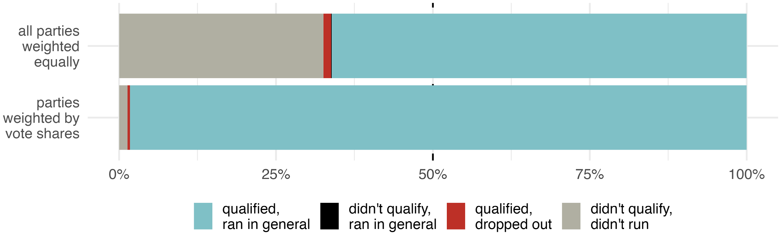
Roughly a third of parties fail to pass the 1.5 per cent barrier, but their combined vote share falls below 2.5 per cent of positive votes (see Figure 2). Voluntarily dropping out is rare: just 1.8 per cent of the 4,421 parties that surpassed the threshold withdrew from the race. ⁹ The EPAOS are thus quite different from run-off systems, in which the election may be decided in the first round or in a second round that is restricted to the top two (sometimes the top three or top four) vote-getters. The point is that EPAOS work more as a comprehensive and easily available pre-election poll than a mechanism for filtering out parties: the combination of mandatory participation with a structured format serves to forecast the frontrunner, the most viable challenger, and the distribution of electoral support among parties more generally. Parties generally retain their primary-election ranking in the general election or move at most just one position up or down (see Figure A3). But this also means that primary results are not fate, and voters and party elites have room for adjusting their behavior and strategies.

Figure 2. Proportion of parties participating in the primary that contested the general election. ‘Qualified’ means that a party obtained at least 1.5 per cent of positive votes in the primary.

Information, Electoral Participation, and Strategic Coordination

Seventy years ago, Duverger (1951) [1967] noted that voters’ awareness of the ‘mechanical’ effect of electoral rules may induce them to abandon parties with little chance of being elected, giving rise to what he called the ‘psychological’ effect of electoral systems. This phenomenon is rooted in the desire to avoid wasting votes. Deriving Duverger’s propositions from a coordination game, Cox (1997, ch. 4) showed that in single-member districts, a Duvergerian equilibrium in which only the top two parties receive a meaningful number of votes requires four assumptions: (a) that small-party supporters are not indifferent between the top-two placed options; (b) that parties and voters seek to maximize their seat share in the current election (rather than sometime in the future); (c) that there is no obvious winner; and (d) that ‘the identity of the trailing and front-running candidates is common knowledge’ (Cox 1997, 78; see also Myatt 2007, 264–5).

The first two assumptions are not information-related and are reasonable for a non-trivial proportion of the electorate in the province of Buenos Aires. However, assumptions (c) and (d) are highly information-sensitive. It is in this context that results from the EPAOS, which provide perfect information about party strength for all parties a couple of months before the general election, can make a difference. ¹⁰ On the one hand, the perceived closeness between the top-placed parties may affect the incentives to both turn out to vote and to do so strategically. Intuitively, the closer the race, the more likely that the effort of turning out will affect the outcome (Shachar and Nalebuff 1999), and that voting for a second-best alternative will prevent the victory of the most disliked option (Cox 1997). Closeness may also heighten emotional engagement – by amplifying enthusiasm, anxiety, or anger – which lowers the psychological cost of voting (Aytaç and Stokes 2019). The implication is that electoral participation should go up, and electoral fragmentation should go down, as the expected competitiveness of the general election increases (Blais 2006). It follows that:

• H ₁. Electoral participation. A smaller margin between the first- and the second-placed party in the primary will increase both (a) turnout and (b) the proportion of positive votes (excluding blank and null ballots) in the general election.

• H ₂. Electoral concentration. A smaller margin between the first- and the second-placed party in the primary will (a) increase the combined vote share of the top-two placed parties and (b) decrease the effective number of parties in the general election.

In addition, primary results also provide information about parties’ ranks: which is placed first, second, and so on. Ranks matter for two analytically distinct reasons. The first is the coordination mechanism central to Duvergerian theory: in order to vote strategically, voters must agree on which are the most viable options. Voters who prefer the third- (or lower-) placed alternative but intensely dislike the frontrunner may strategically shift to the second-placed party (Cox 1997; Fey 1997). For these voters, the runner-up becomes the focal alternative: the option that everyone perceives (and everyone perceives that everyone else perceives, and so on) as the most viable challenger to the frontrunner (Anagol and Fujiwara 2016). Conversely, third-party supporters who dislike the runner-up more than the frontrunner may instead desert to the frontrunner – not out of a desire of supporting the winner, but because a vote for the frontrunner offers the best chance to beat their least-preferred competitor. In both cases, the incentives to abandon the third-placed party intensify as the race between the top-two-placed parties tightens.

Therefore, finishing third rather than second – even by a single vote – should be especially costly: it generates the expectation that the runner-up is the most viable challenger against the frontrunner, prompting voters who dislike it to support the second-placed party instead of the third-placed one (Cox 1997). Thus, other things equal, finishing second rather than third in the primary should provide a boost in the general election:

• H ₃. Focalness. The third-placed party in the primary will (a) suffer an electoral penalty in the general election vis-à-vis the second-placed one, and (b) this penalty will increase the closer the race is between the first- and second-placed parties.

A second, distinct mechanism is rooted not in coordination but in the psychology of ranks: voters may favor higher-ranked options simply because of their position. This may reflect a heuristic through which voters interpret rank as a signal of inherent quality, even if substantive differences between the n ^th- and n + 1^th-placed options are minimal (Anagol and Fujiwara 2016). Another possibility is a bandwagon effect: voters may align with the frontrunner not because they see it as better, but because of the instrumental or psychological benefits of supporting the likely winner. Both experimental studies (Agranov et al. 2018; Hix et al. 2017) and observational evidence (Anagol and Fujiwara 2016; Granzier et al. 2023; Lucardi et al. 2023; Morton et al. 2015) show a tendency to prefer the first-placed party, though this tendency is far from universal (Bursztyn et al. 2024; Chatterjee and Kamal 2021), and weakens or disappears in polarized contests (Granzier et al. 2023; Lucardi et al. 2023). In any case, this mechanism predicts a positive effect of finishing first rather than second, but not necessarily of finishing second rather than third, or third rather than fourth, etc. Therefore:

• H ₄. Bandwagon effect. The first-placed party in the primary will enjoy an electoral boost in the general election.

We finally consider heterogeneous effects. The predictions from Duverger’s (1951 [1967]) propositions are starkest for plurality elections in which there is a single office at stake, and therefore voting for a third party results in a wasted ballot. Under proportional representation (PR), in contrast, voting for a third party does not necessarily mean wasting one’s vote. Municipal elections in Buenos Aires alternate between midterm elections, in which only councilors are elected by PR, and concurrent ones, in which the mayor and half of the local council are elected using a fused ballot – that is, voters are forced to select a mayor and councilors from the same party. Therefore, in concurrent elections, strategic behavior tends to follow the logic of the mayoral race, transforming the entire election into a de facto plurality contest. The fact that mayors are more visible political figures and that the fused vote attaches councilors’ electoral fates to that of their mayoral candidate further reinforces this logic. Even if voters are not aware of the incentives provided by the electoral rules, they certainly see the mayoral election as the highest-stakes one, and the implication is the same. To be sure, this distinction is less stark in practice than in theory; in real-life midterm elections, mayors are often ‘in the background’, promoting their party’s candidates and thus their own support in the local council (Feierherd and Lucardi 2022). To the extent that this is the case, however, we should observe fewer differences between concurrent and midterm elections than if mayors were not involved; in other words, our results should be interpreted as a lower bound.

We also expect to see stronger effects in smaller municipalities. Intuitively, a single individual is more likely to be pivotal in a small district than in a large one (Shachar and Nalebuff 1999). Thus, voters in smaller districts should be more sensitive to electoral closeness and party rankings, either because they realize that by themselves, or because party elites are more persuasive in their mobilization efforts when fewer votes are needed to alter the outcome. ¹¹ In contrast, the bandwagoning logic does not depend on the probability of being pivotal, and thus should not change based on municipality size. Accordingly:

• H ₅. Heterogeneous effects. The relationships predicted in H₁−H₃ should be stronger (a) in concurrent election years and (b) in smaller municipalities.

Closeness, Coordination, and Concentration

Graphical Analysis

Figure 1 shows the evolution over time of both the two margins of interest (1 v. 2 and 2 v. 3) as well as the outcome variables: turnout; the proportion of positive votes; the combined vote share of the two largest parties; and the Golosov (2010) index. ¹² On average, the leading party surpasses the trailing one by 17 percentage points, with substantial variation between municipalities. The difference is somewhat larger in the primary. In contrast, the 2 v. 3 difference increases in the general election, especially during 2001–17, when there was more uncertainty about the identity of the second-placed party. Both turnout and the proportion of positive votes are noticeably lower in the primary.

The combined vote share of the two largest parties and the Golosov index indicate that electoral fragmentation is larger in the primary, especially between 2011 and 2017. This is consistent with voters using primary results to identify, and vote for, the two frontrunners.

Figure 3 examines how the margin between the leading and trailing parties in the primary affects the change in outcome variables between the primary and the general. A closely fought primary increases both turnout and the share of positive votes, though the first relationship is limited to concurrent elections. A smaller margin between the two most voted parties also increases support for the two largest parties: in concurrent years, their combined vote share increases by 4.2 percentage points if they received the same number of votes, but this decreases by 0.13 percentage points for every percentage point difference between them (see Figure 3(c)). In midterm years, the effect is smaller (3.4 and minus 0.093 percentage points, respectively), but still substantial. In very close elections there are between 0.33 and 0.38 fewer effective parties, but this number increases by 0.012–0.013 for every percentage-point difference between the frontrunner and the runner-up.

Figure 3. Primary closeness and change in outcome values between the primary and the general.

Regression Analysis

By looking at the change between the primary and the general election, the plots in Figure 3 account for the fact that outcome values in a given municipality-year may be abnormally high (or low) for reasons that have already manifested in the primary. An alternative strategy is to include municipality and year fixed effects, and thus we estimate models of the form

(1) $$y_{m,t}^{\rm{G}} = \beta \cdot {\rm{margin}}_{m,t}^{\rm{P}} + {\mu _m} + {\delta _t} + {\varepsilon _{m,t}},$$

where $$y_{m,t}^{\rm{G}}$$ is the outcome (in levels) measured in the general election in municipality m in election year t, $${\rm{margin}}_{m,t}^{\rm{P}}$$ is the percentage point difference between the leading and trailing parties in the primary, and μ _m and δ _t are municipality and election year fixed effects, respectively. Since the set of parties participating in the primary and the general election may differ, when computing vote percentages and victory margins in the primary we only include the vote totals of the parties that qualified to take part in the general election (that is, that surpassed the 1.5 per cent threshold) in the denominator. ¹³ To account for floor and ceiling effects, in some specifications we control for the outcome value in the primary, $$y_{m,t}^{\rm{P}}$$ . We cluster standard errors by municipality. All data come from the province’s electoral authority. ¹⁴

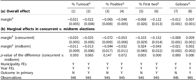
Table 1(a) shows the overall effect for the entire sample. For every percentage point increase in the margin between the leading and trailing parties in the primary, turnout in the general election goes down by 0.021 percentage points – 0.022 if controlling for the lagged outcome – both statistically significant estimates. These effects may seem comparatively small (cf. Arnold 2018; De Paola and Scoppa 2014; Fauvelle-Aymar and François 2006; Garmann 2014; Indridason 2008; Simonovits 2012), but this is likely due to the baseline turnout already being high. ¹⁵ The effect on positive votes in columns (3) and (4) is also negative and significant, but between two and three times larger in size. This is confirmed by the standardized estimates reported in Appendix Table A3: the effect of a (within-municipality) ¹⁶ standard deviation increase in the margin of victory in the primary is two to three times larger for positive votes than for turnout.

Table 1. Between-party closeness in the primary and general election outcomes

Note: Ordinary least squares (OLS) regression estimates. Each panel–column combination reports a different specification. The outcome is always measured in the general election. margin^P is the difference between the percentage of votes of the leading and trailing parties in the primary election, including only parties that classified to the general election in the denominator. Panel (b) reports separate marginal effects for concurrent and midterm elections; the ‘p-value of the difference’ indicates whether these are statistically different from each other. Standard errors clustered by municipality in parentheses.

Where do these additional votes go? Columns (5) and (6) show that for every percentage point increase in the margin between the leading and trailing parties, the combined vote percentage of the two largest parties goes down by between 0.07 and 0.12 percentage points, depending on whether the outcome in the primary is included as a control. Surprisingly, column (7) indicates that this results in a smaller Golosov index – that is, lower electoral concentration in the general election as the primary becomes less competitive – but column (8) indicates that when accounting for the level of concentration in the primary, the sign switches and the effect becomes positive as expected. The standardized results in Appendix Table A3(a) lead to similar conclusions.

Panel (b) compares concurrent v. midterm elections. To make the results more intuitive, we report the marginal effects of the margin of victory in concurrent and midterm elections, as well as the p-values for the difference between the two. The results are much larger – and more likely to be significant – in concurrent elections. That said, the difference in the marginal effect between concurrent and midterm years is only statistically significant at conventional levels for the combined vote share of the largest parties and the Golosov index. Using council size as a proxy for municipality size, Table A2(d) in the Appendix further shows that voters in small districts are more responsive to electoral closeness: in municipalities with six councilors, the impact of closeness on turnout is two to three times larger than in the overall sample. This effect diminishes almost monotonically with increasing council size and becomes negligible in municipalities with 16 or more councilors. The relationship between council size and positive votes is less predictable, however, and there is no clear pattern between council size and the magnitude of the estimated effect for the other two outcomes. The standardized estimates in Appendix Table A3 also support this interpretation.

Robustness

Table A4 in the Appendix shows that for all the variables of interest, the value observed in the primary is a much better predictor than the values from the general elections that took place two or four years before. Looking at the change in the outcome variable between the primary and the general election (Table A5), measuring vote percentages in the primary without removing parties that did not pass the 1.5 per cent threshold from the denominator (Table A6), or taking the natural logarithm of raw votes or the Golosov index instead of vote percentages (Table A7) does not change our findings either. Accounting for intraparty competition in the primary by either (a) splitting the sample depending on which of the top two parties had multiple lists (Table A8) or (b) defining the explanatory variable as the margin between the biggest factions within each of the top two parties (Table A9) also produces similar findings. Neither the incumbent party’s distance to a majority in the council (Table A10) nor district magnitude (Table A11) change the result for midterm elections. ¹⁷

Party Ranks and Coordination

Identification

Determining if a party does better in the general election solely by virtue of having finished in a higher-ranked position in the primary is problematic insofar as better-ranked parties are more popular, nominate more attractive candidates, or control more resources. We thus employ a regression discontinuity (RD) design, comparing parties who finished first instead of second (or second instead of third) by a small margin. Following Calonico et al. (2014), we estimate this effect non-parametrically, fitting a separate regression at each side of the cutoff point of zero and weighting observations close to the cutoff more heavily. For a given outcome variable, we choose the bandwidth that minimizes the estimates’ asymptotic mean squared error (MSE). Since we include two observations for every election, both the density of the running variable and all election-specific characteristics are perfectly balanced by design. We cluster the standard errors by election year to account for the dependency across observations.

Graphical Evidence

The regression discontinuity plots in Figure 4 show the relationship between a party’s margin of victory in the primary and its probability of winning or its vote percentage in the general election. The plots on the left show that the larger the first-placed party’s margin, the more likely it is to win the election and the higher its expected vote share, but there is no visible ‘jump’ at the discontinuity: finishing first in the primary does not confer an electoral advantage of its own in the general election. In contrast, the plot in the top right corner shows that there is an advantage of finishing second: the third-placed party rarely wins the election, but the second-placed one emerges as winner between 10 per cent and 20 per cent of the time, and the difference begins to show up right at the discontinuity. There is no visible effect for vote shares, however. Figures A9 and A10 in the Appendix suggest that these results are driven by concurrent elections and small municipalities.

Figure 4. Mimicking variance regression discontinuity plots with quantile-spaced bins (Calonico et al. 2015) showing the relationship between the margin in the primary and the probability of winning (top) or the expected vote share (bottom) in the general election.

RD Results

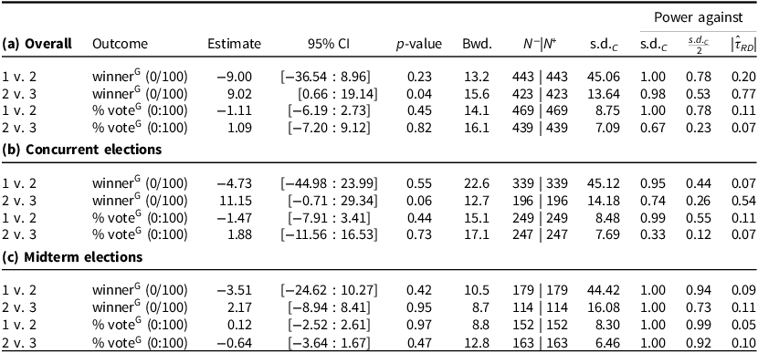
Table 2(a) presents the results for the full sample. Finishing first in the primary has a negative and sizable – minus 9 percentage points – effect on the probability of winning the general election. The estimate is not statistically significant, probably due to low statistical power: as the last three columns of the table show, we generally have 80 per cent power to find an effect as large as a standard deviation of the outcome in the control group (s.d. _C ) and sometimes one half as large (s.d. _C /2), but our RD estimates (|τ̂ _RD |) are usually much smaller than that.

Table 2. Regression discontinuity (RD) estimates: effect of primary ranking on general election outcomes

Note: Sharp (conventional) RD estimates, with robust confidence intervals (CIs) and p-values based on the MSE-optimal bandwidth proposed by Calonico et al. (2014), using a triangular kernel and clustering the standard errors by election year. The running variable is the primary election margin between the first- and second-placed parties (odd-numbered rows) or the second- and third-placed ones (even-numbered rows). Only parties that classified to the general election are included in the denominator. The last three columns report how much statistical power the model has to detect an effect that is as large as (a) a standard deviation of the outcome variable in the control group (s.d. _C ); (b) half as much; or (c) equal in absolute value to the one we actually estimated (|τ̂ _RD |).

In any case, the first-place advantage documented in municipal elections in Brazil (Lucardi et al. 2023) or in legislative elections in France and other European countries (Granzier et al. 2023) does not extend to Buenos Aires. But in line with Anagol and Fujiwara’s (2016) findings for Brazil, Canada, and India, finishing second instead of third provides a 9 percentage point increase in the probability of winning the general election (p=0.04). The estimates for vote shares go in the expected direction – a 1.1 percentage point decrease and increase, respectively – though the small effect sizes and insufficient power means that neither effect is significant. Finding stronger regression discontinuity estimates for winning probabilities than for vote shares is common (see Granzier et al. 2023; Lucardi et al. 2023). On the one hand, we are comparing higher- and lower-ranked parties with very similar vote percentages, and thus even a small change in vote shares may translate into an appreciable increase in winning probabilities. Alternatively, if only a few cases experience large increases in vote shares, the (local) average treatment effect – which is what we estimate – on vote shares may not be that large, but the impact on winning probabilities can be substantial.

The next two panels of Table 2 indicate that the (insignificant) effect of finishing first instead of second does not vary with the electoral calendar, but the second-placed advantage is five times as large in concurrent (11.2 percentage points) than in midterm (2.2 percentage points) years, with a p-value of 0.06 despite the much smaller sample size. This is consistent with theoretical expectations founded on the higher visibility and winner-takes-all nature of mayoral elections vis-à-vis midterm ones. Appendix Table A13 shows that the second-place advantage is larger in the Interior and in small municipalities, with highly significant effect sizes of 14.5 and 20.3 percentage points, respectively. The results for vote shares remain insignificant. This is consistent with expectations, but given the substantial overlap between a municipality’s location and its size – the Interior is home to 88 per cent of small municipalities but just 41 per cent of large ones; 74 per cent of the Interior’s municipalities (but only 20 per cent of the Conurbano’s) are small – we cannot determine if these results are driven by municipality size per se or by the political and demographic differences between the Conurbano and the Interior.

We also expect a larger electoral advantage of finishing second (rather than third) when the first-placed party is within reach – that is, when there is no obvious winner. Figure 5 shows that this is indeed the case: when the distance between the first- and second-placed parties is small – less than 7 percentage points – the premium of finishing second rather than third is around 50 percentage points, far more than the 9 percentage points reported in Table 2(a). Adding less competitive elections reduces this advantage almost monotonically. Figure 5(b) shows that the second-placed party receives a 3–5 percentage point boost to its vote share when it is close to the first-placed party, though these estimates are not significant.

Figure 5. Sharp regression discontinuity (RD) estimates (points) and 95 per cent robust confidence intervals (CIs) (vertical lines) showing the effect of finishing second (rather than third) in the primary on (a) the probability of winning and (b) the vote percentage in the general election, depending on the distance between the leading and trailing party in the primary. The red horizontal lines display the RD estimates and CIs reported in Table 2(a).

Robustness

Again, calculating the running variable using all parties that contested the primary rather than just the ones surpassing the 1.5 per cent threshold does not change the results, though the reduction in power leads to mostly insignificant estimates (Table A14). Another concern is that while we have perfect balance for election-level characteristics, the parties (and candidates) that fall above or below the threshold may differ, for instance in terms of incumbency, alignment with the president (or the provincial governor), or whether they faced a competitive primary. Figure A8 documents some imbalance, especially for party ID characteristics. ¹⁸ This may be due to chance: with 112 tests, we expect 5.6 significant estimates due solely to chance, and find a total of 10. The difference is not worrisome, and in any case Table A15 shows that controlling for all variables included in the balance checks does not change the results. Using a coverage error rate (CER)-optimal instead of a MSE-optimal bandwidth (Table A16) or fitting second-order polynomials (Table A17) produces similar estimates, though the latter are much more variable. The effect of finishing first rather than second is sensitive to bandwidth choice: it begins negative at small bandwidths and then becomes zero or positive, depending on the outcome, though the estimates are never significant. In contrast, the estimate for finishing second rather than third remains pretty stable over bandwidths ranging between 5 and 35 percentage points, though the coefficients are sometimes insignificant (Figure A11).

Documenting Voters’ Attention in Municipal Races

To what extent are these results actually capturing strategic mobilization, rather than just picking up some correlated, but different, phenomena? Insofar as (a) voters care more about national or provincial elections than local ones, and (b) the electoral technology used in Buenos Aires discourages split-ticket voting (Barnes et al. 2017), outcomes for national, provincial, and municipal elections will be correlated. In particular, if voters first make a decision about the national or provincial race and then vote similarly in the municipal one, the previous results may be an artifact of the fact that municipal, provincial, and national elections are held on the same day.

In this section, we offer evidence against this possibility. As Argentina’s largest province, elections in Buenos Aires receive substantial media attention. National newspapers like Clarín, La Nación, Página/12, and Perfil typically provide detailed infographics and interactive maps through which readers can easily access electoral results, even at the local level. Local media like La Noticia 1, El Día, and Radio Provincia offer thorough local-level reporting both before and after election day. Figure 6 validates this interest using Google Trends to measure the relative popularity of the Spanish terms for ‘president’, ‘governor’, ‘mayor’, and ‘councilor’ between 1 January and 31 December of each election year. ¹⁹ Search popularity clearly peaks around the primary and the general elections. Consistent with the assumption that voters do not care much about the local council, interest in ‘councilor’ is low throughout the year and only peaks modestly in some midterm years (2013 and 2017). Searches for ‘mayor’, in contrast, clearly peak around the primary and the general election, but only in concurrent years. Interest in ‘governor’ is comparable to that of ‘mayor’, only without the peaks, while searches for ‘president’ are naturally much more numerous and peak both at election time and when a new president assumes office. While illustrative, these trends support the assumption that voters are informed about the competitiveness of the local race, especially in concurrent elections. Further strengthening this claim, Figure A6 in the Appendix shows that the list of top 10 searches in the seven days immediately after the primary is populated by election- and politician-related terms.

Figure 6. Relative popularity of the Spanish terms for ‘president‘, ‘governor’, ‘mayor’, and ‘councilor’ in Google searches in the province of Buenos Aires, 2011–23. The dashed vertical line indicates the primary election date.

For a more systematic test, we used precinct-level data from 2013 to 2023 to construct a ‘municipal’, ‘provincial’, and ‘national’ version of each of our explanatory and dependent variables. ²⁰ The former are defined as before (though using provisional precinct-level data; see note 20); the latter are similarly constructed, but using results from provincial and municipal elections. For example, margin^P _provincial is the percentage point difference between the two parties that received the most votes in the provincial primary in a given municipality – which may not correspond to the two most voted-for parties in the province. margin^P _national and the outcome variables are similarly defined. ²¹

Figure A7 in the Appendix shows that with the exception of turnout, the within-municipality correlation between these variables is positive, but not overwhelmingly so. If anything, results for provincial and national elections are much more strongly correlated between them than with municipal values. A higher correlation for turnout makes sense, as voters who show up at an election precinct are counted as voting for all offices simultaneously; the only way to participate in one election but not another is if voter rolls are not identical – in particular, foreigners who are permanent residents may vote in municipal elections but not in national or provincial ones.

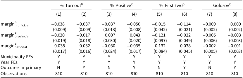
The weaker correlation for the other variables suggests that the transmission between different levels of election is not automatic. Indeed, the ‘horse race’ regressions in Table 3 show that when the margin of victory in the municipal, provincial, and national election are included simultaneously, only the former have a meaningful and statistically significant impact on the outcome; the latter are smaller in magnitude, insignificant, or have the wrong sign. Furthermore, the point estimates for the municipal margin differ little from those of Table 1(a) – with the exception of turnout, where the effect is much larger. In other words: municipal primary results do a good job at explaining municipal outcomes in the general election, but results from the provincial and national primaries do not. Furthermore, the last two panels of Appendix Table A12 show that the latter do not even do a good job of explaining outcomes in the provincial or national election. This is not surprising: while being the most voted candidate in the municipal race determines who will govern a district, in the gubernatorial and presidential races a vote in any municipality is as good as any other: coordination should arise at the provincial (or national) level, not at the municipal one. For the same reason, the municipal margin in the primary has little effect on the outcomes in the provincial or national races, with the exception of turnout. As we just noted, this happens because voting in the municipal but not the provincial or national election is only possible for foreigners with permanente residency. Importantly for our purposes, however, rather than provincial or national mobilization mechanically explaining the correlations observed in Table 1, it is municipal elections affecting turnout in these races ‘from the bottom up’.

Table 3. Between-party closeness in the primary and general election outcomes – ‘Horse race’ between variables measured at the municipal, provincial, and national levels

Note: OLS regression estimates. Each column reports a different specification. The outcome always corresponds to the municipal results measured in the general election. margin^P is the difference between the percentage of votes of the leading and trailing parties in the primary election, including only parties that classified to the general election in the denominator; the municipal, provincial, and national subscripts indicate to which election the values correspond. Standard errors clustered by municipality in parentheses.

As a final check, in Appendix Table A19 we report regression discontinuity estimates like those of Table 2(a) separately for the municipal, provincial, and national races. ²² The municipal results are very similar to the original ones – in fact, they are actually a bit stronger, but this is entirely due to the fact that we do not have data for 2011 (see note 20). The provincial and national estimates reported in panels (b) and (c), in contrast, are much closer to zero in absolute value, sometimes have the opposite sign, and always fall short of statistical significance even at the 0.10 level.

Conclusion

Unlike media coverage, opinion polls, personal networks, or simply ‘vibes’, which can be biased, too expensive, consciously motivated, or manipulated, the EPAOS provide information about parties’ electoral strength that is both widely accessible and immune to the distortions commonly seen in other tools. In this paper, we show that voters in Buenos Aires use them to make marginal decisions regarding whether to turn out and cast a positive ballot, as well as for whom to vote.

The effects we find are subject to alternative interpretations regarding both who is behind these participation efforts – individual voters v. partisan elites – and whether they reflect a strategic coordination or a naive preference for higher-ranked options. While we cannot give a definitive answer, our findings are consistent with the claim that they are driven by (a) individual voters (b) coordinating behind more viable alternatives. Finding a stronger effect for positive votes – which, unlike turnout, cannot be observed by party operatives (Nichter 2008) – is consistent with voters, rather than elites, making the relevant decisions. So is the fact that many hopeless parties contest the primary (compare the weighted v. the unweighted values in Figure 2), that voluntary dropouts are rare, and that the incumbent party’s distance to a council majority does not matter. The finding that the frontrunner in the primary is disadvantaged (though the effect is not significant), while the runner-up enjoys a boost, fits nicely with a coordination story. The Google Trends data (Figure 6), the ‘horse race’ results from Table 3, and individual-level data from the 2015 presidential election (Weitz-Shapiro and Winters 2019) show that Argentine voters are informed and sophisticated enough to distinguish between different levels of election as well as to infer the identity of the second-placed candidate from primary results.

That said, the fact that voters pay more attention to the national president than to the local mayor (see Figure 6) introduces the issue of the scope conditions of our argument and findings: in what contexts should information matter for electoral engagement and coordination? The existing literature has paid particular attention to electoral rules (Cox et al. 2016; Figueroa 2025; Fiva and Hix 2021) as well as the ideological configuration between the top-placed alternatives (Tsebelis 1988; Willis and Indridason 2025) and the degree of polarization between them (Granzier et al. 2023; Lucardi et al. 2023; Murias Muñoz and Meguid 2021). Our findings suggest that (perceptions of) the distribution of votes between parties also plays a crucial role, and highlight the importance of measuring these accurately before election day, for example with high-quality polls (as in Bursztyn et al. 2024).

On the other hand, at least during the period of interest, most municipalities had a ‘two-and-a-half’ party system: even in midterm years, the two largest parties regularly captured almost 80 per cent of the vote, and the average value of the Golosov index was 2.6 (see Table A1(b) in the Appendix). ²³ When just two parties run most of the show, however, we should expect a substantial amount of coordination to be already ‘baked in’ in the primary, as voters anticipate which parties are the most likely to finish first or second – though the precise margin may be quite uncertain. To the extent that a more fragmented party system increases uncertainty regarding which parties will finish first or second, on the other hand, the information provided by a primary system like the one we study here should have a stronger effect on voter coordination.