Evaluating hyperspectral and machine learning approaches to classify biocontrol-induced damage on water hyacinth (Pontederia crassipes)

Abstract

Water hyacinth (Pontederia crassipes Mart.) is a free-floating aquatic plant native to South America that has spread to nearly 50 countries, becoming one of the world’s most invasive aquatic weeds. In Florida, the biocontrol agents Neochetina eichhorniae and Neochetina bruchi were released in 1970s, while Megamelus scutellaris was released in 2010. Assessing the impact of these biocontrol agents is crucial in evaluating efficacy, distribution, and overall progress in management efforts. The traditional survey and monitoring methods used to evaluate the impact of biocontrol present numerous challenges in data acquisition, especially in remote areas and aquatic habitats. This study aimed to detect damage caused by Neochetina spp. and M. scutellaris on P. crassipes using hyperspectral remote sensing. Plants were exposed to varying levels of Neochetina spp. and M. scutellaris herbivory for 2 and 4 wk under laboratory conditions. After the exposure period, the plants were scanned using a visible and near-infrared hyperspectral imaging system. Two classification algorithms, partial least-squares discriminant analysis (PLS-DA) and support vector machine (SVM) were employed for classification. SVM achieved high classification accuracy at both low and high damage levels, with overall training and validation accuracies of 84.9% and 78.79%, respectively, while PLS-DA only achieved high classification accuracy at high damage levels, with overall training and validation accuracies of 56.3% and 60.38%. Based on the observed performance metrics, both algorithms demonstrated improved classification accuracy as damage increased over time. The results indicated that hyperspectral remote sensing can be used to monitor and assess biocontrol agents damage on P. crassipes.

Management Implications

The application of hyperspectral remote sensing in detecting biocontrol damage provides a promising approach for managing Pontederia crassipes (water hyacinth). The two classification algorithms employed, partial least-squares discriminant analysis (PLS-DA) and support vector machine (SVM), achieved high classification accuracy, with an overall accuracy of 80.77%. Based upon qualitative and observed differences in performance metrics, both models improved in classification as biocontrol damage increased over time, suggesting the model’s ability to learn from patterns and relationships in the data. This study demonstrates that integrating hyperspectral remote sensing with machine learning algorithms offers a promising approach for monitoring and assessing the impact of biocontrol agents. Hyperspectral remote sensing has the potential to help managers monitor and assess the impact of biocontrol on P. crassipes and may provide solutions to the challenges and limitations associated with traditional methods in aquatic systems.

Introduction

Pontederia crassipes Mart., commonly known as water hyacinth, is a free-floating plant that produces purple flowers. It is native to South America but has spread to nearly 50 countries and has become one of the world’s most invasive aquatic weeds (Ilo et al. 2020; Penfound and Earle 1948). Pontederia crassipes causes extensive damage by covering large water bodies, altering aquatic habitat by reducing dissolved oxygen and light penetration, and blocking access to agricultural and recreational activities (Villamagna and Murphy 2010). In Lake Okeechobee, FL, USA, P. crassipes has been a problem since 1905, forming dense mats that impede access to navigation and reduce flood control (Langeland and Jacono 2012).

In the United States, four biocontrol agents were released for the control of P. crassipes. Two weevils, Neochetina eichhorniae and Neochetina bruchi (Coleoptera: Curculionidae), a moth, Niphograpta albiguttalis (Lepidoptera: Crambidae), and a planthopper, Megamelus scutellaris (Hemiptera: Delphacidae) were released in 1972, 1974, 1977, and 2010, respectively (Winston et al. 2014). Also existing in Florida are two generalist herbivores, Samea multiplicalis (Lepidoptera: Crambidae) and Elophila obliteralis (Lepidoptera: Crambidae), whose host range includes P. crassipes (Knopf and Habeck 1976). Additionally, Orthogalumna terebrantis (Acarina: Galumnidae), a gallery-forming mite native to South America, was adventively introduced into United States and now occurs in Louisiana and Florida (Bennett 1970; Cordo and DeLoach 1976).

Assessing the impact of biocontrol agents on their target species is an important part of a biocontrol program, as it identifies problems in areas where agents are underperforming and justifies continued funding for biocontrol (Maron et al. 2010). This strengthens control by allowing for the use of additional agents or the development of alternative control strategies (Maron et al. 2010; Reid et al. 2008). Among herbivores on P. crassipes, Neochetina spp. and M. scutellaris have proven to be highly damaging. For example, in Florida, USA, N. eichhorniae caused a 58.2% reduction in plant biomass and a 97.3% reduction in inflorescences (Tipping et al. 2014). Another study reported that M. scutellaris caused 66.9% reduction in biomass (Tipping et al. 2011). Despite this significant reduction in biomass, P. crassipes coverage remained high at 71.1% (Tipping et al. 2014). The persistence in coverage may be attributed to low insect density, with M. scutellaris averaging 10 insects m⁻² (Goode et al. 2021), whereas in South Africa, a study on inundative releases of M. scutellaris reported an average of 6,000 insects m⁻², decreasing P. crassipes coverage from greater than 37% to less than 6% over two consecutive years (Coetzee et al. 2022).

Detecting and monitoring both Neochetina spp. and M. scutellaris infestation levels is imperative in understanding their interactions and efficacy in managing P. crassipes. However, the traditional survey and monitoring methods used in assessing the impact of biocontrol presents numerous challenges in data acquisition, especially in remote areas and aquatic habitats (Rew et al. 2006). Traditional methods rely on ground-based visual surveys such as physical searches via transects, grids, or points (Rew et al. 2006; Zuberi et el. 2014). These methods are costly and time-consuming in large areas (Dube et al. 2014; Rodgers et al. 2018). Additionally, observer errors in detecting, identifying, and estimating the cover of a species may exist (Lepš and Hadincová 1992). The use of hyperspectral remote sensing provides potential solutions for the limitations of traditional methods. Hyperspectral sensors allow the estimate and spatial mapping of constituent chemistries of canopies, allowing for the tracking of fine-scale changes in plant responses to biotic and abiotic stressors at landscape scales (Lassalle 2021). Laboratory-based hyperspectral studies are an important first step in understanding the application and potential of remote sensing in detecting and monitoring the impact of biocontrol on invasive species. It also allows for the control of environmental variables that could confound spectral signature and establish a high-quality spectral library. The aim of this study is to detect damage caused by Neochetina spp. and M. scutellaris on P. crassipes using hyperspectral remote sensing and classification algorithms under laboratory conditions.

Materials and Methods

Plant Preparation

Pontederia crassipes plants were collected from wild populations at Ten Mile Creek Preserve (27.4048°N, 80.3991°W), Fort Pierce, FL. The plants were soaked in soapy water for 1 h using Dawn Professional® (Procter & Gamble, Cincinnati, OH) soap at a concentration of 5 ml L⁻¹ of water and were rinsed with tap water to remove any surface insects or other arthropods. Plants were then placed in aquatic tanks (Rubbermaid® stock tank (Newell Brands, Atlanta, GA), 1.29 by 0.78 by 0.63 m) that were filled with water, in a screenhouse at the Biological Control Research and Containment Laboratory, University of Florida, Indian River Research and Education Center (IRREC), Fort Pierce, FL. An organic mosquito dunk (Summit Mosquito Dunks®) (Summit Chemical Company, Baltimore, MD) was placed in the rearing tank to prevent mosquito larva growth. The active ingredient of the mosquito dunk used, Bacillus thuringiensis israelensis (Bti), is specific to mosquitos and other dipterans and has no effect on any of the biocontrol agents used in this study. A fertilizer floater (made from shade cloth and a pool noodle) was used to distribute fertilizer to floating plants. A mixture of Osmocote® (Israel Chemicals Ltd., Tel Aviv, Israel) fertilizer and iron chelate (12-9-15 Osmocote® at a rate of 0.31 g L⁻¹ water; sequestrene 330Fe chelated iron [10%, powder] at a rate of 0.02 g L⁻¹ water) (Goode et al. 2022), was placed into the fertilizer floater, and the floater was released into the aquatic tank. Fertilizer was replaced in the floater every 3 mo. The tanks were sprayed with safer soap (M-Pede®, Gowan Company, Yuma, AZ) at a concentration of 20 ml L⁻¹ every 2 wk to keep any insects off the plants. The plants were allowed to grow and reproduce vegetatively in the tank. Young plants were then collected and carefully inspected for the presence of larvae or feeding damage, and only insect-free plants were used in the experiment.

Insect Rearing

Adult Neochetina spp. weevils were collected from wild populations at Ten Mile Creek Preserve, Fort Pierce, FL, before the start of the experiment. The two species were not distinguished from each other, as both are well established in Florida. All weevils collected were kept in colonies in small aquatic tanks (11 by 12 by 16 cm) with P. crassipes plants for use in experimentation. Megamelus scutellaris were collected from laboratory colony, from the USDA-ARS Invasive Plant Research Laboratory, Fort Lauderdale, FL, and brought to the IRREC. Megamelus scutellaris were placed on insect-free P. crassipes plants in small tanks, and the same rate of fertilizer noted earlier was applied. All M. scutellaris were reared on P. crassipes plants in small tanks under laboratory conditions, and adults were collected for the experiment.

Impact of Insect Feeding in the Lab

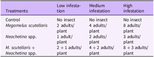
To produce P. crassipes plants with the low, medium, and high levels of impact from Neochetina spp. and M. scutellaris to use in the hyperspectral remote sensing experiments, a randomized complete block design with four treatments and six replications was used. The insect densities corresponding to each impact level (Table 1) were based on field observations and a preliminary study we conducted. Insect-free P. crassipes plants, with short, bulbous, and spongy petioles were collected from the rearing tanks and were soaked in soapy water and rinsed with clean water as described earlier. Three plants of similar size were randomly selected and assigned to a treatment (Table 1). The plants were placed in a small tank filled with 5 L of water. Two drops of Aqua Blue^TM (Pond Champs, Fort Wayne, IN) were added to the water to prevent algal growth, and a mixture of Osmocote® fertilizer and iron chelate was placed loosely in the tanks. An artificial light source (KingLED King Plus 2000W Full Spectrum, Guangzho KingLED Lighting Technology Company, Guangzho, China ) was installed at the top of the study area to provide illumination from evening (6:00 PM) until morning (6:00 AM). The insects were added to the plants following the assigned treatment and allowed to feed and reproduce for 2 or 4 wk before hyperspectral scanning. All insects remained in place until the scan was completed.

Table 1. Treatments with number of adults released per plant^a.

^a Three plants of similar size were placed in each tank before insect release.

Plant Scanning

Plant scanning was conducted at the Agricultural and Biological Engineering Department of the University of Florida, Gainesville, FL, using a Scanning Plant IoT Facility (SPOT). SPOT is a multifunctional high-throughput plant phenotyping platform (Lantin et al. 2023). It has three main sensors: (1) an imaging spectrometer (Nano-Hyperspec®, VNIR, 400–1000 nm, Headwall Photonics, Bolton, MA), (2), a thermal camera (FLIR Vue Pro R, Teledyne FLIR, Wilsonville, OR), and (3) a LiDAR camera (RealSense^TM LiDAR Camera L515, Intel, Santa Clara, CA). SPOT’s imaging spectrometer collects imaging data at high spectral resolution (∼2 nm), allowing for discrimination of plant responses to various stressors (Lantin et al. 2023). SPOT is equipped with four incandescent bulbs that are fixed relative to the imaging sensor to provide uniform lightning across the Nano-Hyperspec’s field of view. SPOT is equipped with a Spectralon® reflectance panel (Spectral Evolution, Haverhill, MA) for enabling relative radiometric calibration of collected imagery. All sensors are mounted pointing nadir (directly downward) above the scanning region.

For this experiment, three plants (one replicate) were placed in a 50.8 by 38.1 by 17.78 cm plastic container (Polypropylene Traex® ColorMate™, United States Plastic Corp., Lima, OH ), containing 3 L of water to allow them to float, simulating natural field conditions. For each scan, the plastic plant container was placed under SPOT along the X scanning direction and the Spectralon® reflectance panel was placed at the start of the scan position with its height adjusted to the average height of the canopy using a tripod. Once scans were obtained, the imagery were converted to apparent at-surface reflectance and processed as described in the following section.

Image Processing

The raw imagery obtained from the SPOT facility was processed to analysis-ready data for assessing plant damage. The images were first converted from digital numbers to at-sensor radiance using the factory calibration coefficients supplied with the sensor. Subsequently, radiance spectral values were divided by reference reflectance spectral values collected from the Spectralon® panel to convert imagery to apparent at-surface reflectance. All radiometric calibrations were performed using SpectraView v. 64.5.5.1 (Headwall Photonics).

Once images had been preprocessed, we extracted reference spectra from the images by visually identifying pixels signifying healthy plants, non-insect damage, biocontrol damage, and background regions. Reference spectra were extracted from all treatments, and given the limited dataset for each infestation level, treatments were grouped and classification was performed at the treatment level.

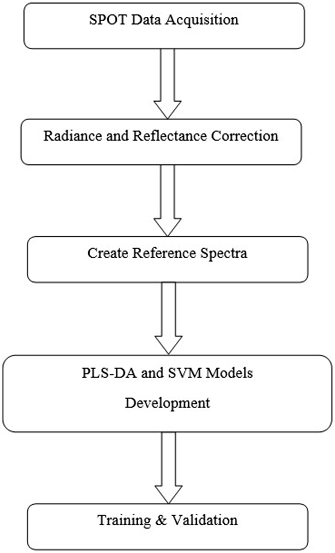
The reference spectra were then used to classify the pixels into different classes using partial least-squares discriminant analysis (PLS-DA) and support vector machine (SVM) algorithms. All analyses were conducted using the R statistical computing environment, R v. 4.3.0 (R Core Team 2023). We followed a standardized image processing workflow depicted in Figure 1.

Figure 1. Image processing flowchart, from data acquisition and processing through model training and validation. PLS-DA, partial least-squares discriminant analysis; SPOT, Scanning Plant IoT Facility; SVM, support vector machine.

Classification Algorithms and Statistical Analysis

Hyperspectral classification algorithms PLS-DA and SVM were used to classify changes in spectra caused by feeding damage between the two biocontrol agents. PLS-DA is an algorithm used for discriminatory variable selection as well as predictive and descriptive modeling. It is derived from the classical partial least-squares regression (PLSR) method for constructive predictive models (Wold et al. 2001). PLS-DA is capable of handling complex data and can resolve spectral and spatial similarities and reduce background effect across species (Peerbhay et al. 2013). PLS-DA has been used in discriminating forest species (Sibiya et al. 2021), crop disease (Shi et al. 2018), and mapping of invasive species (Lottering et al. 2020) and is especially relevant for spectroscopy applications, as it accounts for multicollinearity between predictors.

SVM is a supervised learning model used for classification and regression (Mountrakis et al. 2011). SVM offers a classification technique that uses a geometric criterion rather than a purely statistical criterion (Melgani and Bruzzone 2004) and can handle small training datasets, producing higher classification accuracy (Perna and Burrows 2005). SVM employs the structural risk minimization approach for class member discrimination, which reduces classification error on unseen data without making previous assumptions about the data’s probability distribution (Mountrakis et al. 2011). For the classification, the data were split into 80% for training and 20% for validation, and both PLS-DA and SVM models were trained and validated using the training and validation sets.

We also employed partial least-squares (PLS) and principal component analysis (PCA) to discriminate between Neochetina spp. and M. scutellaris damage by examining clustering of samples according to spectral variation. PLS and PCA are dimensionality reduction techniques that transform data from high-dimensional space to low-dimensional space (James et al. 2013). PLS uses between-groups sums-of-squares and cross-products matrices for dimensionality reduction, while PCA depends on the sample variance/covariance matrix (Barker and Rayens 2003).

Results and Discussion

Visual Observation of Megamelus scutellaris and Neochetina spp. Damage on Pontederia crassipes after 2 and 4 Weeks of Exposure

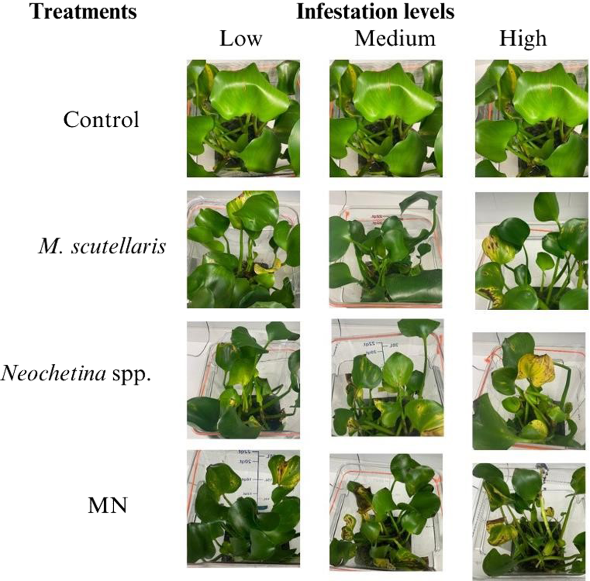
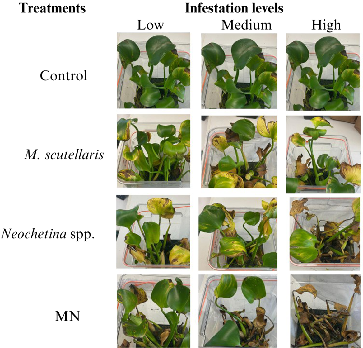
Pontederia crassipes plants were assessed through visual observation, and damage was classified based on severity: none (0% damage), mild (1% to 25%), moderate (26% to 50%), and severe (>50%). Plants exposed to M. scutellaris, Neochetina spp., or the combination of M. scutellaris and Neochetina spp. showed moderate to severe damage after 2 and 4 wk of exposure. After 2 wk of exposure, the combined treatment of M. scutellaris and Neochetina spp. at high infestation showed more damage than either of the treatments alone. In all treatments, plants produced new leaves that were fresh and buoyant (Figure 2). However, after 4 wk of exposure, all biocontrol treatments across all infestation levels showed severe damage, with yellowish, brown, and black discoloration, and lost vigor and buoyancy. Mortality was observed in plants at high infestation levels of Neochetina spp. (3 adults per plant) and the combined treatment of M. scutellaris and Neochetina spp. (Figure 3). Plants in the control treatment appeared healthy, vigorous, and buoyant, with new growing leaves and a few old leaves showing yellowish hues resulting from senescence.

Figure 2. Damaged Pontederia crassipes plants exposed for 2 wk to varying levels of Megamelus scutellaris, Neochetina spp., and their combination (MN). Note that an image of the same plant is shown in the control row for illustrative purposes.

Figure 3. Damaged Pontederia crassipes plants exposed for 4 wk to varying levels of Megamelus scutellaris, Neochetina spp., and their combination (MN). Note that an image of the same plant is shown in the control row for illustrative purposes.

Under field conditions, feeding damage typically becomes apparent after several weeks and increases over time (Jones et al. 2018). This pattern is likely due to the abundance of host plants and low insect density. In contrast, the controlled setup of this study amplified the effects of feeding, as limited plant biomass and close proximity of the insects to each other and to their food source accelerated visible damage.

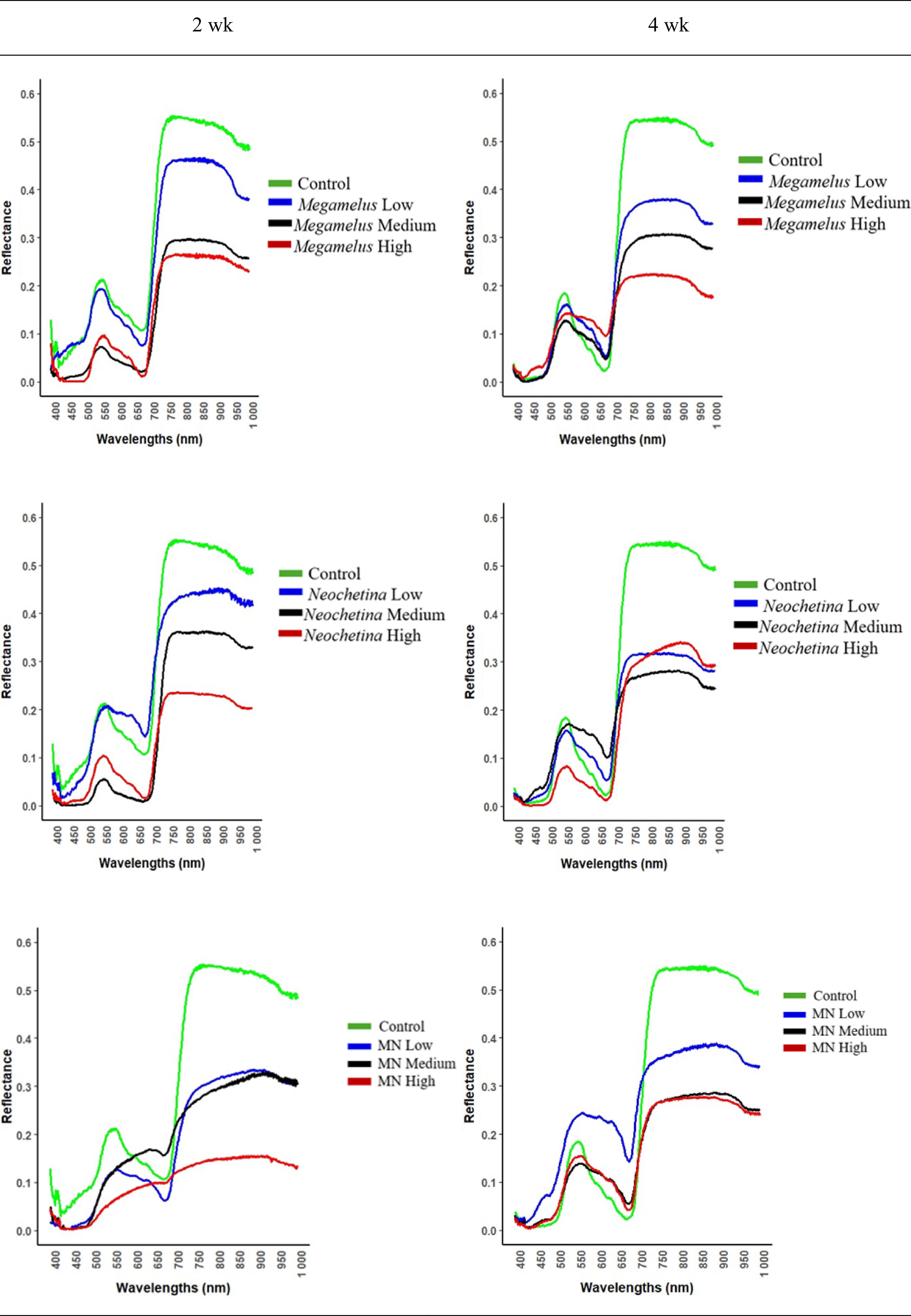
Spectral Reflectance of Megamelus scutellaris and Neochetina spp. Damage on Pontederia crassipes after 2 and 4 Weeks of Exposure

The spectral reflectance observed across all biocontrol treatments demonstrated a consistent trend after 2 and 4 wk of exposure (Figure 4). In an examination of the spectral reflectance of individual treatments, the control and low infestations generally exhibited higher spectral reflectance compared with medium and high infestations. However, for the combined treatment at 2 wk of exposure, the low and medium infestations showed similar spectral reflectance, while the medium and high levels showed similar spectral reflectance after 4 wk of exposure.

Figure 4. Spectral reflectance of Megamelus scutellaris and Neochetina spp. damage on Pontederia crassipes. Left: 2 wk of exposure; right: 4 wk of exposure. MN, combined treatment of M. scutellaris and Neochetina spp.

When all treatments at 2 and 4 wk of exposure were compared (Figure 4), the control treatment consistently exhibited higher spectral reflectance in the near-infrared region (∼750 to 900 nm), suggesting healthier plant tissue. However, these differences were less pronounced in the red region (∼650 to 700 nm), particularly during the 4 wk of exposure. In contrast, biocontrol treatments at high infestation levels showed stronger absorption in the blue region (400 to 550 nm), indicating stress and potential changes in foliar biochemistry due to damage caused by biocontrol agents.

PLS-DA and SVM Classification

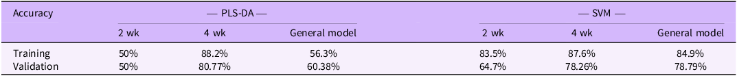
The classification was performed at treatment level using PLS-DA and SVM algorithms. Training and validation accuracy were initially obtained separately for the 2 wk and 4 wk data, and the data were later combined to assess accuracy for the general model. Given the limited dataset for each infestation level, treatments were grouped, and classification was performed at the treatment level. The overall classification accuracies for the models are presented in Table 2. Results indicated varying levels of effectiveness between the two classification algorithms across different time periods. The results showed that SVM outperformed PLS-DA for the 2 wk of exposure and the general model, which combines data from the 2 and 4 wk of exposure. SVM achieved higher training and validation accuracy for the 2 wk of exposure and the general model compared with PLS-DA. However, after the 4 wk of exposure, PLS-DA achieved higher training and validation accuracy than SVM. Due to a limited sample size, statistical analysis was not performed to assess the significance of the difference. Overall, the performance of SVM and PLS-DA was almost equal, demonstrating the effectiveness of both methods for classification. The training and validation values increased qualitatively over time, reflecting increasing skill in detection as the infestation progressed.

Table 2. Partial least-squares discriminant analysis (PLS-DA) and support vector machine (SVM) training and validation accuracy for 2 and 4 wk of exposure and the general model^a.

^a The general model integrates both datasets for a comprehensive accuracy assessment.

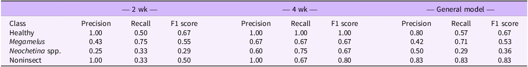
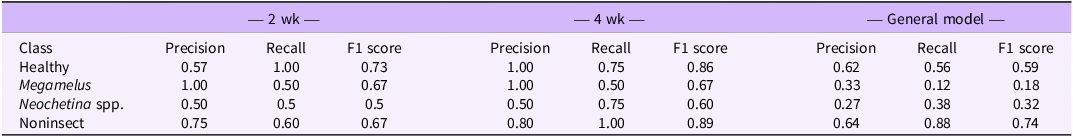
To better understand the model performance for each damage class, we further analyzed per-class precision, recall, and F1 score. The per-class performance metrics indicated how well the model predicts each damage class: healthy, M. scutellaris, Neochetina spp., and non-insect damage. The results for PLS-DA (Table 3) and SVM (Table 4) demonstrated strong predictive power, with both models performing well across all classes. The performance qualitatively improved from 2 wk of exposure to 4 wk of exposure but declined in the general model, a trend also observed in overall classification accuracy. A trade-off between precision and recall was also observed, where high precision comes at the cost of recall and vice versa, highlighting the importance of considering the F1 score as a balanced performance metric.

Table 3. Per-class precision, recall, and F1 scores for partial least-squares discriminant analysis (PLS-DA) models based on 2 and 4 wk of exposure and the general model^a.

^a The general model integrates both datasets for a comprehensive assessment of classification performance.

Table 4. Per-class precision, recall, and F1 scores for support vector machine (SVM) models based on 2 and 4 wk of exposure and the general model^a.

^a The general model integrates both datasets for a comprehensive assessment of classification performance.

The classification results for SVM (Table 2) demonstrated the robustness of the algorithm in classifying biocontrol damage on P. crassipes. SVM outperformed PLS-DA in accuracy, even at lower damage levels (training: 83.5%; validation: 64.7%), while PLS-DA only achieved high classification accuracy at high biocontrol damage (training: 88.2%; validation: 80.77%). The results align with the findings of Abu-Khalaf and Salman (2014). The performance of PLS-DA at low damage levels may be affected by the low signal-to-noise ratios, making it difficult to distinguish subtle differences between classes. However, as damage increases, the signal improves, enhancing classification performance (Ruiz-Perez et al. 2020). Both PLS-DA and SVM effectively classify images with high accuracy due to their robustness. PLS-DA is effective in handling multicollinearity in high-dimensional data with small sample size, provides high prediction, and is robust to noise (Dumancas and Bello 2015), while SVM is flexible and exhibits strong generalization capabilities, making it an effective tool for classification (Wang and He 2004). Studies have reported the effectiveness of PLS-DA and SVM in classifying different levels of insect herbivory (Huang et al. 2014; Wang et al. 2023) and plant disease severity (Abu-Khalaf and Salman 2014). For example, Wang et al. (2023) employed four spectral data processing techniques (Savitzky-Golay smoothing, multiplicative scatter correction, first derivative, and standard normal variate transformatio) and three classification algorithms (SVM, logistic regression, and PLS-DA) to identify and classify insect-infested maize (Zea mays L.) seeds, achieving highest classification accuracy of 0.86 and 0.88 for PLS-DA and SVM, respectively. Ekramirad et al. (2022) classified codling moth, Cydia pomonella (Lepidoptera: Tortricidae) infestation in apple cultivars using four classification algorithms and reported PLS-DA as having the highest classification accuracy. In this study, training and validation accuracy for both models qualitatively increases as damage to P. crassipes increased over time. This suggests that as biocontrol damage increased, the model’s ability to learn also improved, thereby enhancing classification accuracy. The ability of classification algorithms to improve accuracy over time has also been reported in previous studies. For example, Agjee et al. (2016), used random forest (RF) to detect biocontrol efficacy in P. crassipes and reported a reduction in RF error by 19.79% between week 1 and week 5. Similarly, Furuya et al. (2021) employed different algorithms, including SVM, to detect insect damage in maize and reported an improvement from day 1 to day 5, with the highest classification achieved on day 5. These findings demonstrated the ability of classification algorithms to learn from pattern and relationship over time. In P. crassipes, studies have shown that biocontrol damage increases with time (Coetzee et al. 2022), resulting in significant physiological and morphological stress that alters the spectral reflectance of the plant (Agjee et al. 2015).

Performance of PLS-DA and SVM Model versus Number of PCA Components

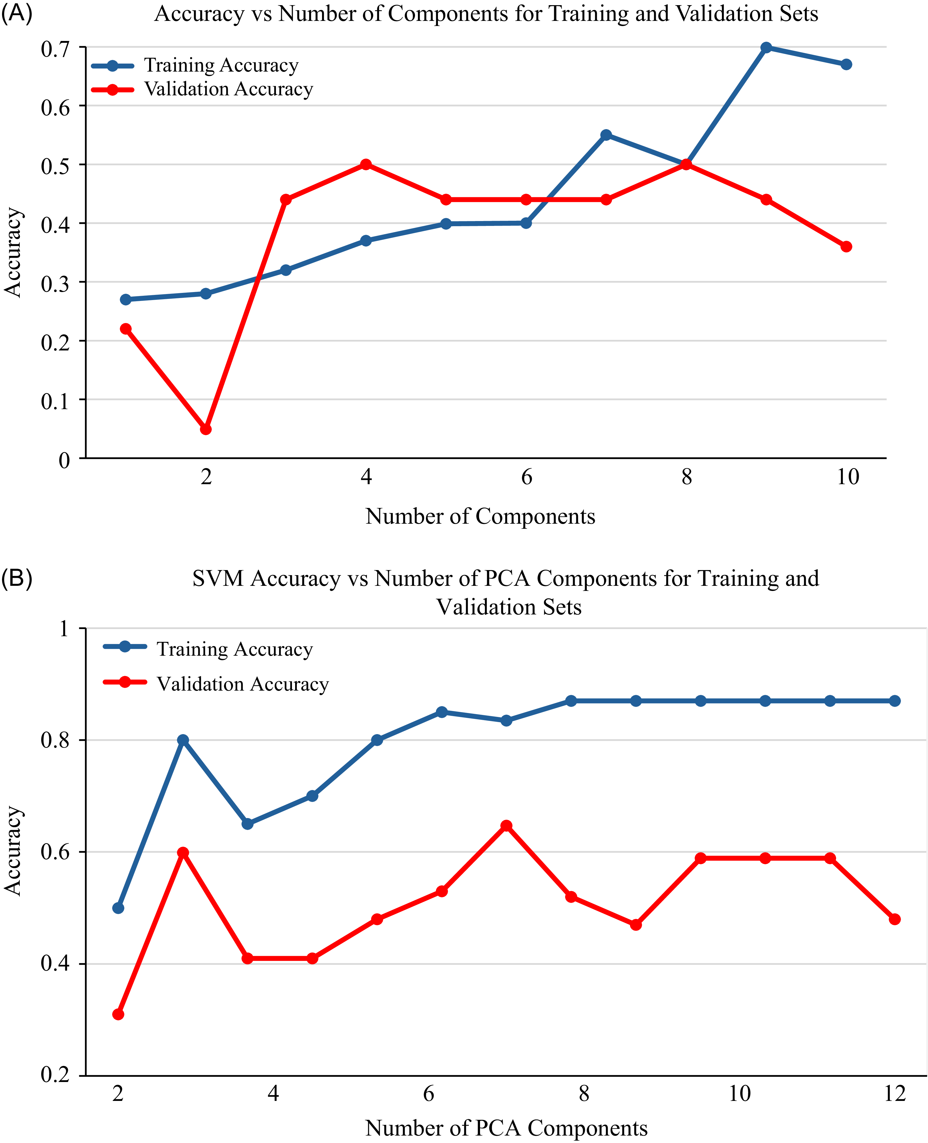
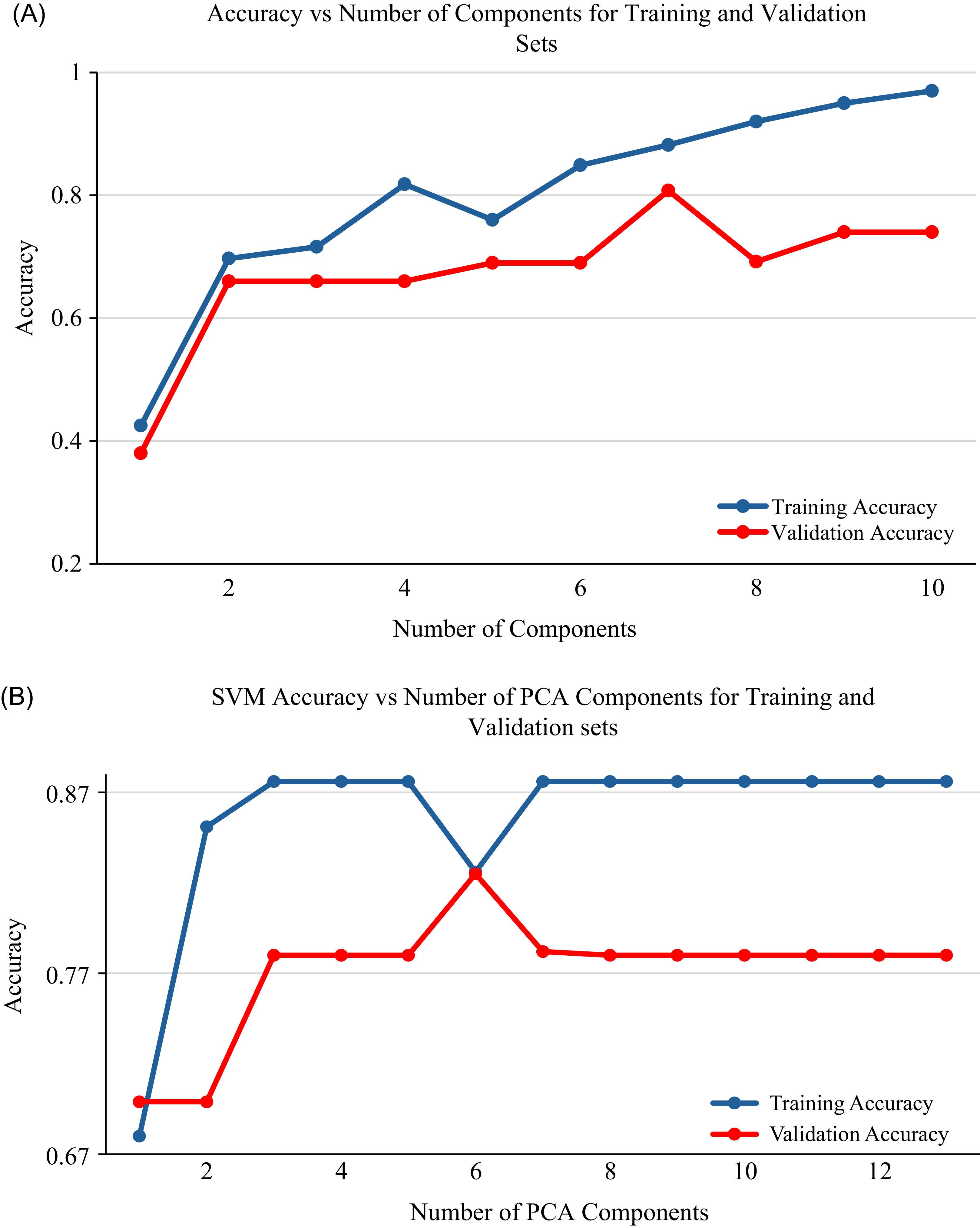
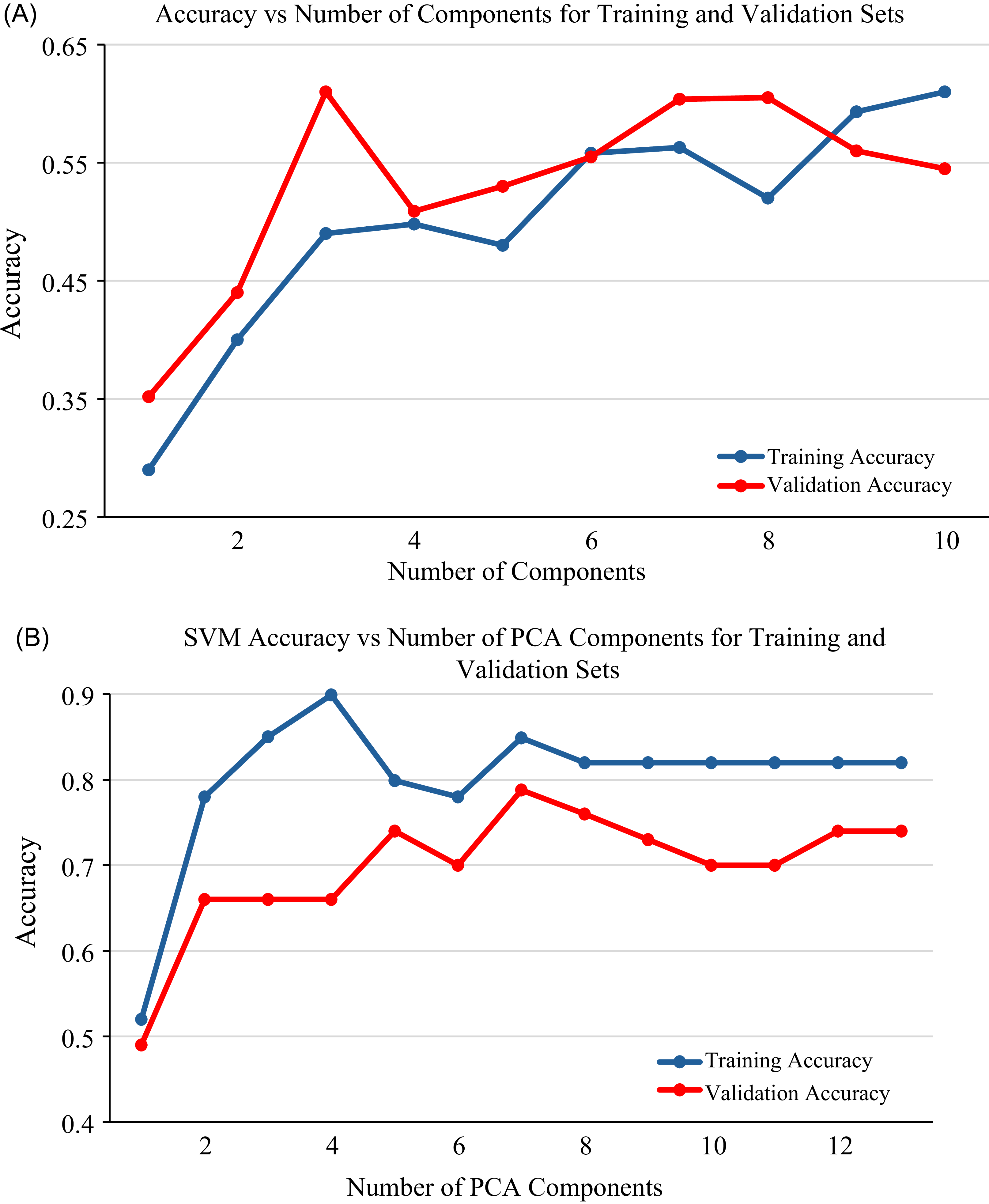
Training and validation accuracy of PLS-DA and SVM models in relation to the number of PCA components are presented for 2 wk of exposure (Figure 5), 4 wk of exposure (Figure 6), and the general model (Figure 7). Both the PLS-DA and SVM models demonstrated a consistent trend, in which training and validation accuracy fluctuate as the number of components increases. Initially, the accuracy of the models increased with an increase in the number of components from 1 to 8, demonstrating the benefit of an increase in components and the ability to capture relevant patterns. However, when the number of components increases above eight, the training accuracy tends to stabilize, indicating a potential for overfitting if more components were to be added. For both models, seven principal components were identified as optimal, providing the highest accuracy and low variance. An exception to this was observed for the PLS-DA model at 2 wk of exposure, in which eight principal components showed the highest accuracy and low variance. While the increase in number of components can improve classification (Vrigazova 2021), there is a maximum number of components beyond which accuracy declines (Bonab and Can 2019). This highlights the intricate relationship between accuracy, the number of components, and model complexity.

Figure 5. Training and validation accuracy vs. number of principal component analysis (PCA) components for 2 wk exposure: (A) partial least-squares discriminant analysis (PLS-DA) and (B) support vector machine (SVM).

Figure 6. Training and validation accuracy vs. number of principal component analysis (PCA) components for 4 wk of exposure: (A) partial least-squares discriminant analysis (PLS-DA) and (B) support vector machine (SVM).

Figure 7. Training and validation accuracy vs. number of principal component analysis (PCA) components for the general models: (A) partial least-squares discriminant analysis (PLS-DA) and (B) support vector machine (SVM). The general model integrates both datasets for a comprehensive accuracy assessment.

PCA transforms spectral data into uncorrelated principal components, capturing the most variance in the data (Bro and Smilde 2014). It is an effective technique that highlights significant patterns and analyzes spectral relationships (Bro and Smilde 2014; Jolliffe and Cadima 2016). Each principal component can be analyzed independently, providing an overview of the data structure and demonstrating the relationship between the objects (Kamruzzaman et al. 2013). In this study, principal components 7 and 8 provided the highest training and validation accuracy for both PLS-DA and SVM. The training and validation accuracy show a consistent pattern, in which accuracy fluctuates as the number of components increases and then declines with a continued increase in the number of components. This pattern demonstrated how well the models fit as the number of components varies. The effectiveness of PCA can vary across different studies. For example, Aigbokhan et al. (2022) and Salata and Grillenzoni (2021) reported that the first several components contain the most relevant information and provide high classification accuracy, while others, such as Zheng and Rakovski (2021), argued that omitting lower-order components can reduce classification accuracy. The findings of this study highlight the effectiveness of PCA in both dimensionality reduction and classification, emphasizing that the selection of principal components should be based on research objectives and other relevant factors.

PLS and PCA Data Analysis

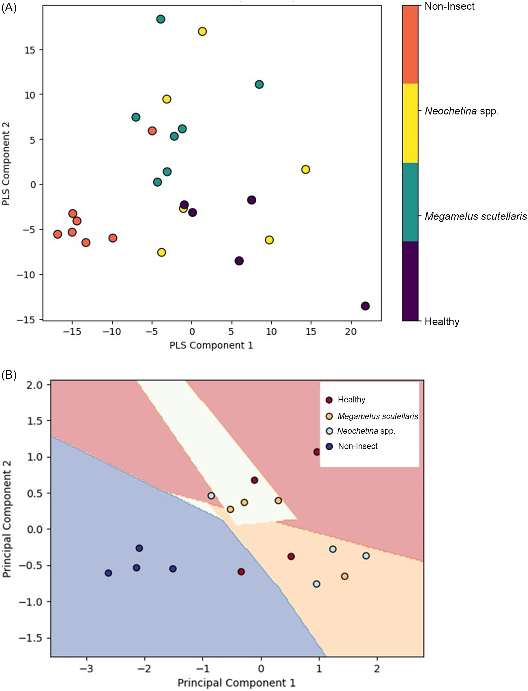
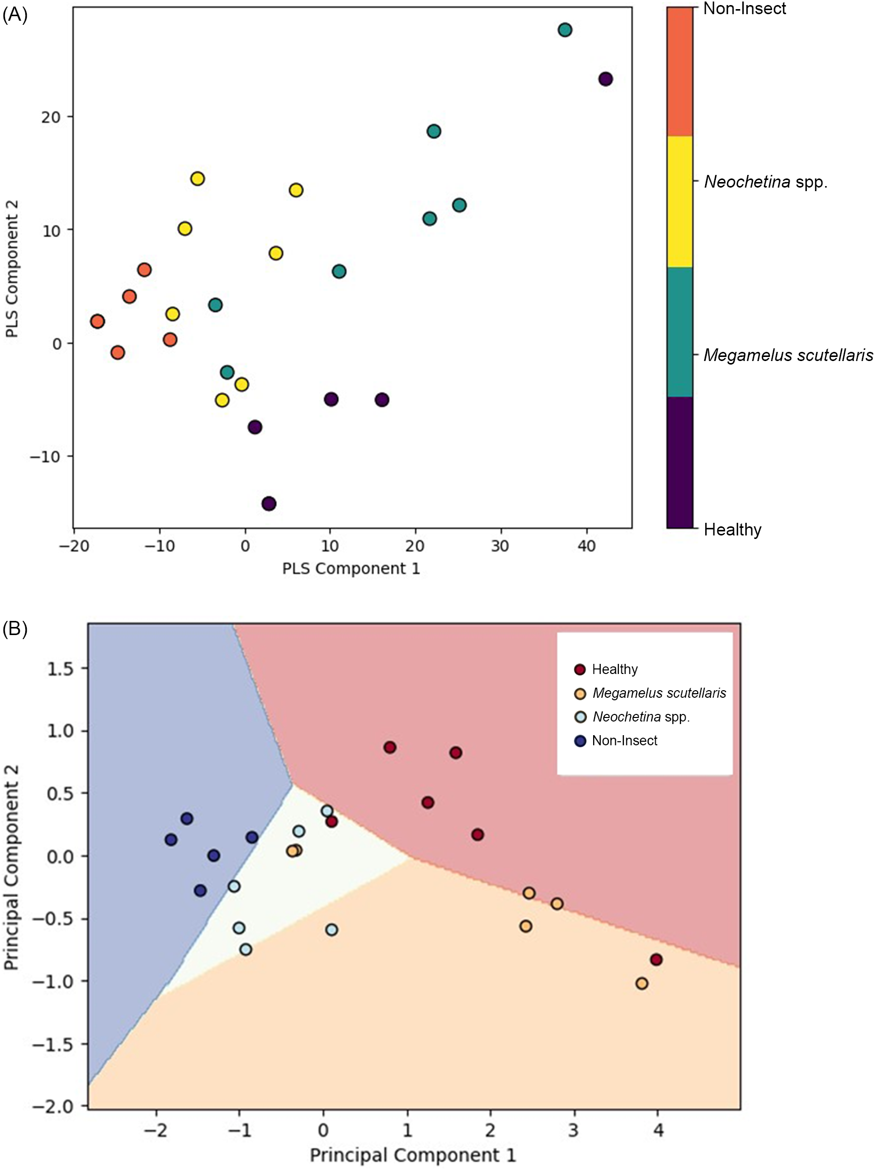
PLS and PCA were used to visualize and analyze spectral data. PLS was integrated with PLS-DA, while PCA was integrated with SVM to highlight properties, grouping, and similarities and to identify contrast by determining the most significant direction based on the spectral feature of the sample (Barker and Rayens 2003; Kamruzzaman et al. 2013). The spectral data were converted into score and loading vectors using PLS analysis and PCA (Barker and Rayens 2003; Huang et al. 2014). PLS-PLSDA and PCA-SVM were performed separately for 2 wk of exposure (Figure 8), 4 wk of exposure (Figure 9), and the general model (Figure 10). Both models indicate that each class was located in distinct region in the plot. The non-insect damage and healthy classes are clustered closely in their respective regions, while Neochetina spp. and Megamelus scutellaris are scattered. The non-insect classes are regions collected from old leaves that display yellowish hues not caused by insect damage, while the healthy classes are taken from control plants with no signs of damage. The non-insect classes were included to reduce the risk of misclassifying natural leaf aging as insect-related damage. The scattering observed in Neochetina spp. and M. scutellaris classes reflects the heterogeneity and varying infestation levels within these groups. Additionally, there was some minor overlap between the two classes in both models, particularly in the general model, highlighting the challenges faced in accurately classifying these classes. Overall, PLS outperformed PCA, demonstrating clearer separation and less overlap among classes, suggesting the effectiveness of PLS in using correlation between independent variables and dependent variables to enhance classification performance.

Figure 8. Score plots for 2 wk of exposure: (A) partial least squares (PLS) and (B) principal component analysis (PCA).

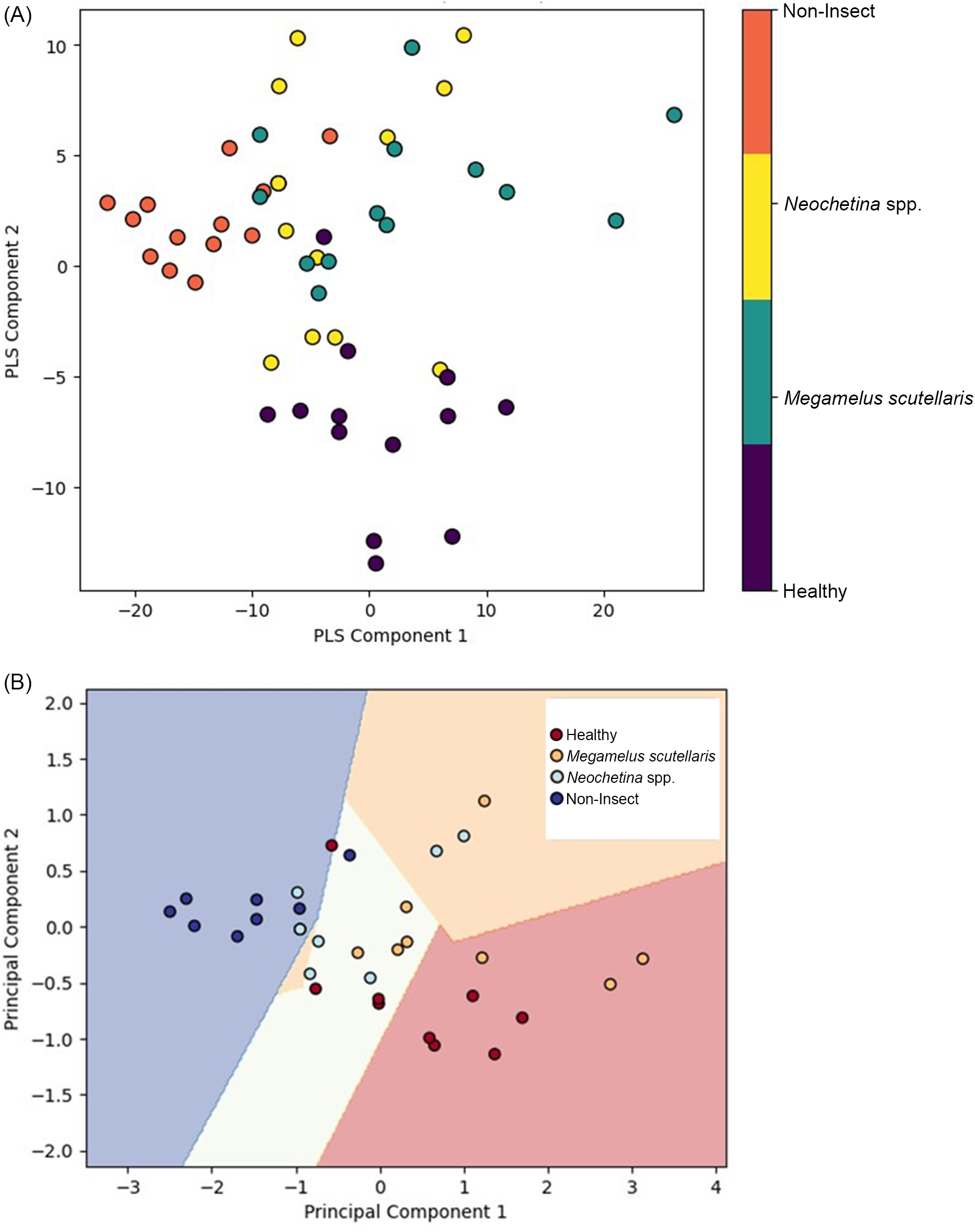
Figure 9. Score plots for 4 wk of exposure: (A) partial least squares (PLS) and (B) principal component analysis (PCA).

Figure 10. Score plots for the general model: (A) partial least squares (PLS) and (B) principal component analysis (PCA). The general model integrates both datasets for a comprehensive accuracy assessment.

The results of the PLS analysis and PCA showed qualitatively similar patterns for 2 wk, 4 wk, and the general model. The score plots illustrate the relationship between samples and the differences in performance between the models. The non-insect and healthy classes are clustered together, suggesting homogeneity in features, while Neochetina spp. and M. scutellaris are more scattered, indicating variability in infestation levels. PLS demonstrates a clearer separation compared with PCA. This has also been reported by Kemsley (1996) and Barker and Rayens (2003). However, as variability increases, PCA may lose important classification information (Barker and Rayens 2003; Zheng and Rakovski 2021). Additionally, score plots show some overlap between the Neochetina spp. and M. scutellaris classes in both models. The variability and overlap observed may result from different infestation levels, similarities, and low damages at lower infestations levels. However, as damage increases over time, discrimination between the classes improves.

In comparison with traditional methods, which are labor-intensive, costly, and time-consuming, hyperspectral remote sensing provides high spectral resolution (Arasumani et al. 2021), enabling early detection and discrimination of varying levels of biocontrol damage. This laboratory study lays the groundwork for identifying unique spectral signatures under a controlled environment. The limited dataset and reliance on qualitative metrics in this study may have affected the robustness of the findings. Future research should expand upon this study and address these limitations by employing larger datasets, incorporating quantitative measures, and utilizing techniques such as cross-validation or bootstrapping and hyperspectral sensors mounted on unmanned aerial vehicles (UAVs) for field-based detection.