1 - Introduction

Summary

In this introductory chapter, we briefly go over the definitions of terms and tools we need for data analysis. Among the tools, MATLAB is the software package to use. The other tool is mathematics. Although much of the mathematics are not absolutely required before using this book, a person with a background in the relevant mathematics will always be better positioned with insight to learn the data analysis skills for real applications.

About Chapter 1

In this introductory chapter, we briefly go over the definitions of terms and tools we need for data analysis. Among the tools, MATLAB is the software package to use. The other tool is mathematics. Although much of the mathematics are not absolutely required before using this book, a person with a background in the relevant mathematics will always be better positioned with insight to learn the data analysis skills for real applications.

1.1 Some Definitions and Concepts

1.1.1 About Data

In most parts of this book, by data we specifically mean a time series or a set of time series – numbers or vectors in a sequence obtained through time from measurements, numerical model simulations, or predictions using certain methods or algorithms from computation by some theory or formula. In other words, data here are generally a series of numbers (usually real numbers) or a series of vectors that are lined up in time, i.e. each element in the series (either a number or a vector) is associated with an independent time stamp. Occasionally, we discuss data without an explicit time stamp (e.g. coastline data). Here, a vector is a group of independent numbers or variables such as the velocity components $u,v,w$ defined in a three-dimensional space and time. A vector can also be a more abstract collection of variables with different units, e.g. the so-called phase space in statistical physics in which the instantaneous state of a system with $n$ particles is described by the coordinates of all n particles and the velocities of the $n$ particles ($x_1$, $y_1$, $z_1$, … , $x_n$, $y_n$, $z_n$, $u_1$, $v_1$, $w_1$, … , $u_n$, $v_n$, $w_n$). This kind of vector is often seen in empirical orthogonal function (EOF) analysis. When a time series is discussed, we either imply that there is a series of time stamps associated with a series of numbers or vectors, or the data include explicitly the time stamps with a series of numbers or vectors.

Occasionally, data might be complex number time series with real and imaginary parts (the imaginary part is the product of a real number and $i=\sqrt{-1}$). In this book, we mostly work with real number time series. However, we will also work with complex number series in two subjects, especially the first subject: (1) Fourier analysis (Davis, 1963): when we do Fourier analysis and fast Fourier Transform for a time series, complex numbers are often introduced for operational computation purposes, although in theory that is not absolutely needed; (2) rotary spectrum analysis: in oceanography, for two-dimensional flow velocity vector time series, we sometimes use a technique called rotary spectrum analysis, which is a special kind of Fourier analysis for vector time series to examine the spectra of velocity in terms of the cyclonic and anticyclonic rotations. In this kind of analysis, the horizontal velocity components are expressed in a complex form for mathematical convenience ($w=u+iv,i=\sqrt{-1}$), taking advantage of the Fourier series in exponential form using the Euler formula $e^{ix}=\cos x+i\sin x$.

1.1.2 Function vs. Discrete Series of Numbers

Data are collected at discrete time instances and/or locations. For that reason, we sometimes use the phrases digital data and discrete data. Digital data is perhaps used more often to mean that data are saved in a “digital” form in a computer. In the context of discussion here, there is no difference between a data file saved in a computer and a data file with numbers written on a piece of paper. The point is that time series data are not “continuous” in the mathematical sense. However, we use a lot of theories and results from mathematical work on continuous functions. Of course, a continuous function is simply an idealized simplification and cannot be realized in real life, particularly in scientific data. No matter how fast one samples, there is always a finite sampling interval, and the data is discrete rather than continuous.

This intrinsic discontinuous nature of data does not really affect our application of mathematical results derived from studies on continuous functions. However, we sometimes do say something like “this time series has a discontinuity.” That can be concluded by a quick eye-ball observation of the data file or a more sophisticated and objective computer-based scan of the data with certain criteria. This is, unfortunately, subjective. There may be an unusual outlier in the data that appears to be unreal due to instrument failure or some unexpected influence of other environmental factors. For example, say a water-level sensor is deployed at the bottom of an estuary, measuring the water level at an hourly interval. A storm arrives, and some strong waves unexpectedly push the instrument into a 5 m deeper water despite the fact that the instrument may be heavy and would not move under normal conditions. The data file would record at the next hourly data point an increase of 5 m in water level. The sudden jump is obviously “discontinuous.” Of course, if the instrument is securely installed, this jump may not happen. But the reality is not always ideal. An instrument normally considered to be securely mounted may not be secure anymore if there is a record-breaking storm. The judgment of whether there is a discontinuity in a data file depends on the nature of the data under study and the experience of the person who does the analysis. Usually, a quick QA/QC with defined rules would be able to find “discontinuity” points in the given time series data.

1.1.3 Time Series vs. Spatial Series

Can numbers in space rather than in time be included in the analysis for either theoretical or application purposes? In general, yes. For instance, using the Fourier Transform as an example, instead of having variations expressed in time that can be converted into the frequency domain, a series of real numbers for different positions in space (i.e. spatial series) can be converted into the wavenumber domain. A spatial series can be in a one-dimensional, two-dimensional, or three-dimensional space, and thus the wavenumber can be either a scalar or a vector.

Our focus here in this book is time series, although at times we discuss the analysis of spatial data or space–time mixed data. In a sense, when one understands clearly time series analysis, it should become easier to understand spatial series analysis. Of course, these two types of data can be very different. One cannot simply use the time series analysis methods on spatial series without considering their differences. For one difference, a time series is ordered naturally from a start time (earlier) to an end time (later). Data in space, however, are not necessarily ordered “naturally.” For example, for data defined on a rectangular grid, we could order the data according to the rows, or columns, or any other peculiar way. After all, spatial data may not be always given on a nice, rectangular grid. The data points could be totally random in distribution.

Full coverage of the analysis of spatial data is not within the scope of this book. In this book, we only include some aspects of the techniques dealing with data obtained in space, such as those obtained from a moving platform. Strictly speaking, they are not necessarily a pure spatial series – they are data mixed in time and space because a moving vessel’s speed is limited.

It should be noted that we will discuss a method of analysis, the empirical orthogonal function or EOF analysis, which involves data mixed in time and space, or a collection of time series defined at different locations. As an example, a series of satellite images for the same region falls into this category – for each image, it presents a spatial series, but for each position in the region, there is a time series provided by the sequence of the images.

1.1.4 The Time Stamps and Time Intervals

When we are working with time series, the order of the sequence of numbers is important because that provides information about variations in time (e.g. an event or a trend) that determine the rate of change in time. We are interested in the variations, though the average values can be important as one parameter. How a measured or simulated variable would change with time (or space, for spatial series) is what we are often interested in.

To calculate the rate of change in time, we must have information about the unit of time and time intervals of the data. Therefore, a time series of temperature, for instance, is not just a series of temperature values but also a series of time values with a proper unit that goes side-by-side with the temperature values that are measured or defined at those times.

For time series data, the time intervals between data points can vary. It is more convenient in many applications that the time series data are obtained at constant time intervals. This is often the case with modern instruments that collect data automatically with a built-in microprocessor or mini-computer and data logger. In this case, and also in the case of model output of time series data, some data files might ignore explicit time stamps; however, information about time intervals and start time with proper units must be provided either inside the data file or separately, depending on the designer of the data collection device or the programmer of a computer model and nature of data (e.g. whether a uniformly spaced time series data or not).

Many of the data analysis techniques are directly applicable only to uniformly spaced data with constant time intervals. Otherwise, some treatment such as interpolations or resampling needs to be done first. There are some exceptions to this. For one example, the general least squares method does not require that data points are equally spaced in time. A specific example in oceanography is the tidal harmonic analysis, which does not require that the data have constant time intervals. Harmonic analysis is based on the least squares method. The following is an example of time series of velocity vector at 2-minute intervals.

Year	Month	Day	Hour	Minute	Second	VE (cm/s)	VN (cm/s)
2016	04	05	21	32	56	−1.1	1.1
2016	04	05	21	34	56	−2.6	2.8
2016	04	05	21	36	56	−5.1	4.0
2016	04	05	21	38	56	−10.4	8.5
2016	04	05	21	40	56	−8.3	7.9
2016	04	05	21	42	56	−5.5	4.8
2016	04	05	21	44	56	−5.0	3.7
2016	04	05	21	46	56	−4.8	3.7
2016	04	05	21	48	56	−13.2	9.8
2016	04	05	21	50	56	−10.9	7.4
2016	04	05	21	52	56	−6.7	3.9
2016	04	05	21	54	56	−4.6	2.7
2016	04	05	21	56	56	−3.0	1.1
2016	04	05	21	58	56	−2.7	0.4
…

Each line corresponds to one record of data from observations at a given time instance. Here the time stamps (the first six columns) are provided. The last two columns give the east and north components of velocity in cm/s. Alternatively, the data could have been provided without the first six columns, but the starting time and time intervals have to be provided for the time series data to be meaningful. For observational data, it is probably better to have the time stamps included explicitly for each record to avoid mistakes because real observations, especially the raw data files, often have gaps for various reasons. If the time stamp is not explicitly included in a data file for each record (or each sample), a single gap can mess up the entire dataset by introducing misalignment in time. With proper time stamps, after reliable quality control of the data, the gaps could be filled. For constant interval data, inclusion of the time stamps will make the data file larger. If data file size is to be minimized, the time stamps can be omitted, given that the start time and time interval are provided in the data file or with the data file. This is often practiced for saving numerical model output files, which can be extremely large.

1.1.5 Oceanographic and Other Data

By oceanographic data, we intend to limit our discussion to data of oceanic origin, i.e. those obtained from the ocean or coastal and estuarine waters. This, however, should not be taken too narrowly as far as the data analysis techniques are concerned. Generally speaking, the methods discussed in this book can be applied to data from other disciplines. For instance, the fundamental methods of analysis for atmospheric data should be very similar, if not the same. There would be no essential differences. The atmospheric and oceanic time series data sometimes need to be analyzed together, e.g. for storm surge problems, in which the atmosphere provides the forcing (air pressure, wind stress, precipitation), while ocean and coastal waters respond to the forcing. Oceanographic data do indeed have some unique aspects that are pertinent mainly, if not only, to the ocean dynamics. For example, tides occur in the ocean, and we will discuss the tidal analysis (i.e. the abovementioned harmonic analysis). Although there is a tidal signal in the atmosphere known as the atmospheric tide, harmonic analysis is usually meant for the ocean only. The technique, however, is applicable to the atmospheric tide as well.

1.1.6 The Tool We Use: MATLAB

MATLAB is a commercial software package that is suitable for calculations and related visualizations of vectors (one-dimensional), matrices (two-dimensional), and arrays (one-, two-, or multidimensional). Although the methods of analysis are independent of the computer programs that implement them, we use MATLAB exclusively in this book. It has many choices of mathematical tools. For example, it has specialized tools for Signal Processing and Wavelet Analysis Toolboxes, which we may need to use at some point in this book. MATLAB is easy to learn and use, and yet has lots of powerful capabilities. Alternative computer languages and or software packages also exist, e.g. IDL, R, C, C++, FORTRAN, Python, etc. Many resources on these computer languages are available online or in publications, but we only use MATLAB throughout this book for consistency and simplicity.

1.2 Background Knowledge

To learn the materials in this book well, some background knowledge in mathematics and physics and related basic skills are preferred, though a high-level skill of any of these subjects is not necessarily required. The subjects of study, particularly in terms of the techniques in this book, are quite broad. Background knowledge includes linear algebra, calculus, Fourier theorem, numerical analysis, and some basics of statistics. In addition, oceanographic data analysis is often aimed at the resolution of dynamical processes in the ocean. Therefore, some background knowledge in e.g. physics, fluid dynamics, and tidal theory would also help to understand some of the techniques (e.g. rotary spectrum analysis and tidal harmonic analysis). Assumptions are made here that the readers have some basic background knowledge of these subjects, but efforts have been made to provide enough information as standalone materials. Some selected basic information and review of background theories are provided in the book for convenience. Intuitive interpretations may be provided for a better understanding when some background information is discussed.

1.2.1 Linear Algebra

Linear algebra is a branch of mathematics dealing with arrays of numbers. A time series of a quantity is itself a special case of an array. Linear algebra includes theories and methods of solving linear sets of equations. This provides the basis for many data analysis techniques, such as linear regression, Fourier Transform, and harmonic analysis. Knowledge in linear algebra makes it much easier to work with matrix operations, which are the major backbone of MATLAB. MATLAB is best suited for working with vector, matrices, and arrays. Linear algebra with matrix operations greatly simplifies the mathematical expression of concepts. These simplifications are implemented by the design of MATLAB language, while inside MATLAB the computer is directed to do the heavy lifting for detailed calculations. With a combination of the two (simplified concepts and MATLAB), our brain power can be reserved for interpretation of the results instead of the details of the actual calculations.

1.2.2 Calculus

Calculus is an important branch of mathematics about the rate of change of functions (differentiation) and the inverse calculations of differentiation (integration). It is the mathematical backbone of almost all disciplines in modern physics. Calculus is fundamental to many theories and techniques of analysis and number crunching, in many ways. This can be seen mainly in two examples in this book: one is Fourier Transform, in which the basic knowledge of integration and linear independence of base functions will help greatly. Similarly, the least squares method is also based on the theory of calculus. The optimal solution of the Fourier coefficients or best fit in the least squares method is a great product of calculus. Another example of the application of calculus is Taylor series expansion, which is very useful in laboratory experiments for error estimations. The beauty of Taylor series expansion is that it can approximate an arbitrary differentiable function to any accuracy (at least in theory) by a polynomial, which is one of the simplest general functions one can find. In addition, the theories for the empirical orthogonal function and wavelet analysis are also based on calculus. Without calculus, none of these techniques would have been invented.

1.2.3 Fourier Theorem

Fourier theorem is the basis for the technique we discuss extensively in this book: the Fourier analysis. Although we will provide relatively complete, albeit brief, coverage of the theory, it will help if the readers have learned the subject before. The importance of Fourier theorem to time series analysis can be compared to that of Newton’s Second Law to mechanics. This may be an overstatement, but the point is, Fourier theorem provides a great leap in understanding the characteristics of a function – in our case, a function of time. The theorem basically guarantees that, except for a peculiar function with infinite discontinuity points, a general (arbitrary) piece-wise continuous function that only has a finite number of finite-range jumps can be expressed (decomposed) in terms of a series of sine and cosine functions of different scales. Here, scales are either in terms of frequency for time series or wavenumber for spatial series.

In the case of a time function, if the length of time of the function is finite (which is usually the case, because no real observations can be infinitely long, except in idealized thought experiments), the series of sine and cosine functions generally are discrete in terms of the scales (discrete frequencies or wavenumbers), although there are infinite numbers of them. These (infinite number of) discrete sine and cosine functions are called the base functions. The series itself is called the Fourier series. The Fourier theorem tells us that such an infinite Fourier series converges to the original function in an averaged sense. Here, “average” means the average of the right and left limits of the function at one point, obtained by approaching from the right of the point and that the left of the point. In other words, at any point (or time, for time function) where the function has a finite discontinuity, the Fourier series converges to the average of the two points on both sides of the jump – i.e. the middle of the jump. If the function at the point is continuous, these two limits are the same. That is, if the function is continuous, the Fourier series will converge to the function at that point.

The Fourier theorem also helps us to understand the effect of finite sampling, such as the highest frequency that can be resolved (i.e. the Nyquist frequency), the frequency resolution, and the artificial oscillations or Gibbs Effect. The properties of the Fourier series allow a wide applicability and an extension into the Fourier Transform.

1.2.4 Numerical Analysis

Numerical analysis deals with some practical methods and techniques of calculations using computers, such as root finding from a nonlinear equation, interpolation and techniques using polynomials, numerical differentiation, numerical integration, calculations in linear algebra, and numerical solutions for ordinary differential equations. An example of relevance to time series analysis in this book is an understanding of interpolations, although we will not discuss the theories of interpolations; we will, rather, rely on just MATLAB’s built-in functions for interpolations. Interpolations are oftentimes among the first steps of data processing, before conducting a Fourier Transform or spectrum analysis for a time series obtained from actual measurements from the ocean (or anywhere else). As mentioned earlier, observations usually contain gaps. Interpolations are useful for filling “small” data gaps, in which the gaps between adjacent data points are much smaller than the minimum useful time scales. For large data gaps, interpolation may introduce significant errors. How do we determine if a gap is really “small”? This depends on the problem under discussion. It depends on the significant time scales contained in the signal, time intervals, number of gaps, and length of the gaps. Although actual situations can have an infinite number of possibilities, the decision is usually based on common sense. For instance, for a problem with tidal variations of water level, we have a time series with 10-minute time intervals. For this time series, if there are six consecutive missing data points in a row within a tidal cycle (12-hour period for a semi-diurnal, tide-dominated case), the gap would not pose a major problem; a simple interpolation would fill the data gap without altering the information in any significant way, meaning no major influence on the spectrum or temporal properties. However, if the time interval is 1 hour and there are six consecutive data points missing (e.g. a 6-hour data gap), the time series property and spectrum after an interpolation for that 6-hour gap would be highly questionable. That, of course, also depends on how we do the interpolation: Are we using a linear interpolation, or are we using some functions for the interpolation? The problem with a function is that for real world observations, if data are missing, there is no way we know exactly what happened during the time when valid data were not recorded. Any function used for interpolation is subjective and can never be verified, because what we do not know is exactly whether there was any “event” during the time with missing data. If we have additional information, e.g. observations from an adjacent position, then the story will be completely different, as then we might be able to assume a certain relationship for the interpolation based on the additional information.

1.2.5 Statistics

Statistics is needed here and there in the book. Statistics, however, can arguably be a double sword in this context. On the one hand, statistics is often needed for analysis on real data because of the intrinsic random nature of observations: real data are functions affected by random processes, at least to some extent. The random processes include intrinsic characteristics of the physical processes, such as chaos in the dynamics or random errors in measurements and systematic errors in instruments. On the other hand, many of the mathematical tools are developed first, without considering the random nature of numbers at all, i.e. only deterministic functions are considered. As we all know, calculus is presented originally and mostly with the differentiations and integrations of deterministic functions rather than random functions. Fourier Transform was also originally developed without any consideration of the randomness of functions. When these mathematical operations are applied to real data, however, the effects of randomness may have to be considered. This will make the problem a little more complicated, but we have to admit that there are some uncertainties, and any estimate will need to take that into account. Having said these, this book is not a statistics book. Some of the analysis will be easier to understand without considering randomness in the beginning. The statistical aspects can be better understood after one has grasped the basics of the techniques developed for deterministic functions.

1.3 About Wind, Current, and Wave Directions in 2-D

In oceanographic data analysis, we often work with two-dimensional vector time series data such as wind, current, and wave, when the vertical components of wind, current, and wave are not considered. Here we discuss and contrast the definitions of directions of two-dimensional wind, current, and ocean waves. It can be confusing as to what the definitions of directions of the two-dimensional wind, current, and wave are. Although two-dimensional wind and currents are vectors that can be expressed in two components (for the horizontal two-dimensional wind and current velocities), they are routinely reported with a magnitude and direction. The direction of wind and that of currents are, however, opposite in definition. It can be confusing and therefore is important that the definitions of these directions are well understood by the data users.

Wind velocity is a vector which tells us where an air parcel at a given location and time is moving to. In theory, wind velocity should have three components in a Cartesian coordinate: the vertical wind velocity component and two horizontal components. The vertical component, however, is not routinely reported unless for special studies of cloud physics, precipitation mechanism, and small-scale atmospheric processes in the troposphere. For this reason, when we talk about the wind direction, we are referring only to that of the horizontal wind velocity. This is the same for current velocity and waves. When the ocean current direction is mentioned, we usually mean that of the horizontal velocity. The direction of propagation of internal waves can be at an angle to the surface. Here we are only referring to the direction of surface waves.

1.3.1 Examples of Wind Data

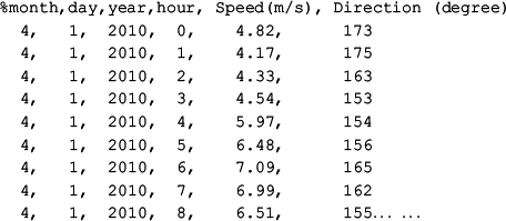
The following shows some sample hourly (horizontal) wind data from an offshore station at (90°32ʹ W, 29°3.2ʹ N) obtained in April 2010.

%month,day,year,hour, Speed(m/s), Direction (degree)
  4,   1,  2010,  0,    4.82,      173
  4,   1,  2010,  1,    4.17,      175
  4,   1,  2010,  2,    4.33,      163
  4,   1,  2010,  3,    4.54,      153
  4,   1,  2010,  4,    5.97,      154
  4,   1,  2010,  5,    6.48,      156
  4,   1,  2010,  6,    7.09,      165
  4,   1,  2010,  7,    6.99,      162
  4,   1,  2010,  8,    6.51,      155… …

The first line is a comment line in MATLAB and is self-explanatory: it explains the data in the following rows and columns, which include time (the first four columns), wind speed in meters per second (the fifth column), and wind direction in degrees (the last column). For wind speed, there should be no vagueness, as it is the wind speed relative to the Earth. For wind direction, there are two questions: what is the reference direction of wind with 0 degrees and how is the angle measured – clockwise or counterclockwise?

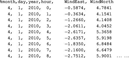
Before we answer these questions, let us look at the following wind data from the same location and same time:

%month,day,year,hour,    WindEast, WindNorth
   4,  1,  2010,  0,     −0.5874,    4.7841
   4,  1,  2010,  1,     −0.3634,    4.1541
   4,  1,  2010,  2,     −1.2660,    4.1408
   4,  1,  2010,  3,     −2.0611,    4.0452
   4,  1,  2010,  4,     −2.6171,    5.3658
   4,  1,  2010,  5,     −2.6357,    5.9198
   4,  1,  2010,  6,     −1.8350,    6.8484
   4,  1,  2010,  7,     −2.1600,    6.6479
   4,  1,  2010,  8,     −2.7512,    5.9001  … …

The only thing different here is that the wind data are provided as the east and north components, rather than the wind speed and wind direction. Both types of wind data are commonly used. Perhaps it is more common to use the speed and direction in observational data and east and north components from model output. Indeed, the standard weather data reported by NOAA and other agencies usually use the first format. The everyday weather forecast on TV and radio uses the wind speed and direction, rather than the east and north components. We say that “the wind tomorrow is predicted to be from the northeast with a maximum speed of 10 knots or 5 m/s,” but not that “the wind tomorrow is predicted to have an east component of negative 7 knots and a north component of negative 7 knots,” which would be awkward and inconvenient if not confusing for the general public.

1.3.2 Definition of Direction of Wind

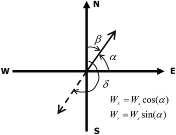
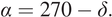
As an international standard, the wind direction is defined as the direction from which the wind comes (therefore, wind direction is the opposite of the wind velocity vector). In some literature, including handbooks, the definition of direction of wind stops here; however, this is incomplete, because this definition does not tell us how the direction is counted – clockwise or counterclockwise – and from where, i.e. what is the 0 direction? To complete the definition, the wind direction is the direction in degrees from which the wind is coming, and the angle is counted from true north (0 degrees is defined from true north) and clockwise (Fig. 1.1). Wind direction is presented as a number in degrees from 0 to 359.9. With this definition, a 45-degree wind is from the northeast. If the wind direction is 90 degrees, it is coming from the east, while 180 degrees is from the south and going to the north.

Figure 1.1 Definition of wind direction. The dashed line with an arrow indicates the wind direction, while the solid line with an arrow shows the wind velocity vector.

1.3.3 Converting between Wind Speed and Direction to Wind Velocity Components

To derive the east and north wind components from the wind data with wind speed and direction, we notice that from Fig. 1.1, the wind direction $\delta$ and the wind velocity vector direction $\alpha$ have the relationship

$\alpha =270-\delta .$(1.1)

This is the angle mapping for wind between wind direction (measured clockwise) and the angle of wind vector relative to the east direction (measured counterclockwise).

The wind vector’s east and north components are then determined by

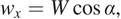$w_x=W\cos \alpha ,$(1.2)

$w_y=W\sin \alpha ,$(1.3)

in which $w_x$, $w_y$, and $W$ are the wind velocity components in the $x$ and $y$ directions and wind velocity magnitude, respectively. Here the positive $x$ and $y$ directions are the east and north directions, respectively.

1.3.4 Definition of Direction of Ocean Current

The direction of ocean current is defined as the direction to which the ocean water goes. Therefore, the ocean current direction is the same as the velocity vector. The ocean current direction is also counted from the north (0 degrees to the north) and measured clockwise. Again, here we are also just referring to the horizontal velocity.

1.3.5 Converting between Current Speed and Direction to Current Velocity Components

Ocean current data is very similar to wind data, such that the data can be given as either current speed and direction (where it goes to) or the east and north components of the horizontal flow vector. We can still use Fig. 1.1 to derive the equations. The only difference is that the ocean current direction is the direction to which it goes, and therefore $\beta$ in Fig. 1.1 is the direction of the ocean current. The corresponding equation to map the angles is

$\alpha =90-\beta .$(1.4)

This is the angle mapping for current between the current direction (measured clockwise) and the direction of current vector relative to the east direction (measured counterclockwise).

The east and north components of the current velocity are determined by

$u=U\cos \alpha ,$(1.5)

$v=U\sin \alpha ,$(1.6)

in which $u$, $v$, and $U$ are the current velocity components in the $x$ and $y$ directions and flow speed, respectively. Here the $x$ and $y$ directions are the east and north directions, respectively.

The following shows some sample data for current obtained from Caminada Pass of Barataria Bay in speed-direction format:

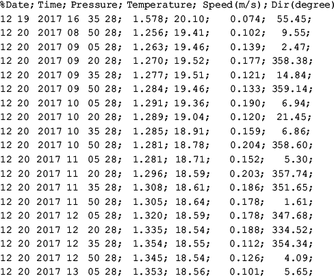
%Date; Time; Pressure; Temperature;  Speed(m/s); Dir(degree)
12 19 2017 16 35 28;  1.578; 20.10;    0.074;  55.45; 
12 20 2017 08 50 28;  1.256; 19.41;    0.102;   9.55; 
12 20 2017 09 05 28;  1.263; 19.46;    0.139;   2.47; 
12 20 2017 09 20 28;  1.270; 19.52;    0.177; 358.38; 
12 20 2017 09 35 28;  1.277; 19.51;    0.121;  14.84; 
12 20 2017 09 50 28;  1.284; 19.46;    0.133; 359.14; 
12 20 2017 10 05 28;  1.291; 19.36;    0.190;   6.94; 
12 20 2017 10 20 28;  1.289; 19.04;    0.120;  21.45; 
12 20 2017 10 35 28;  1.285; 18.91;    0.159;   6.86; 
12 20 2017 10 50 28;  1.281; 18.78;    0.204; 358.60; 
12 20 2017 11 05 28;  1.281; 18.71;   0.152;   5.30; 
12 20 2017 11 20 28;  1.296; 18.59;   0.203; 357.74; 
12 20 2017 11 35 28;  1.308; 18.61;   0.186; 351.65; 
12 20 2017 11 50 28;  1.305; 18.64;   0.178;   1.61; 
12 20 2017 12 05 28;  1.320; 18.59;   0.178; 347.68; 
12 20 2017 12 20 28;  1.335; 18.54;   0.188; 334.52; 
12 20 2017 12 35 28;  1.354; 18.55;   0.112; 354.34; 
12 20 2017 12 50 28;  1.345; 18.54;   0.126;   4.09; 
12 20 2017 13 05 28;  1.353; 18.56;   0.101;   5.65;

Like wind data, ocean current data can be presented in either speed–direction format or east–north format, for the horizontal velocity. It should be noted that it is more common to have the vertical velocity component measured in ocean current data than in the wind data. An acoustic Doppler current profiler (ADCP) usually measures the three-dimensional velocity components, except for the two-beam models, which only measure the horizontal components. Unlike horizontal velocity, the direction of the vertical velocity component is either up or down so there is no question about the definition of direction in the vertical.

1.3.6 Definition of Directions of Waves

For wave data, the definition is similar to that of wind: the direction of waves is defined as that from which the waves are coming. The units are degrees from true north, increasing clockwise, with north as the reference or 0 degrees. Not all wave data have information about the wave direction. Commonly reported wave data include the wave height, wave period, significant wave height or the average of the highest one-third of the wave height, etc. Only the directional wave data include the information about wave direction. Directional wave data are relatively rare. In addition to these wave data formats, spectral wave data are another format, which includes information for different frequencies. In the following, some sample directional wave data are shown. The data are obtained from the National Data Buoy Center (NDBC, www.ndbc.noaa.gov/dwa.shtml).

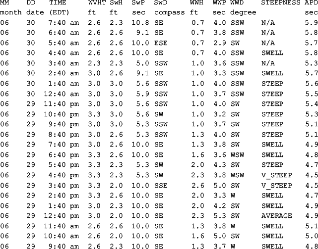
MM    DD TIME WVHT SwH SwP SwD WWH  WWP WWD STEEPNESS APD
month date (EDT)  ft ft sec compass ft  sec degree           sec
06    30   7:40 am  2.6  2.3  10.8 SE      0.7  4.0 SSW    N/A      5.9
06    30   6:40 am  2.6  2.6   9.1 SE      0.7  3.8 SSW    N/A      5.8
06    30   5:40 am  2.6  2.6  10.0 ESE     0.7  2.9 SW     N/A      5.7
06    30   4:40 am  2.6  2.6  10.0 SE      0.7  4.0 SSW    SWELL    5.8
06    30   3:40 am  2.3  2.3   5.0 SSW     1.0  3.6 SSW    N/A      5.3
06    30   2:40 am  3.0  2.6   9.1 SE      1.0  3.3 SSW    SWELL     5.7
06    30   1:40 am  3.0  3.0   5.6 SSW     1.0  4.0 SSW    STEEP     5.6
06    30  12:40 am  3.0  3.0   5.9 SSW     1.0  3.7 SSW    STEEP     5.5
06    29  11:40 pm  3.0  3.0   5.6 SSW     1.0  4.0 SW     STEEP     5.4
06    29  10:40 pm  3.3  3.0   5.6 SW      1.0  3.2 SW     STEEP     5.3
06    29   9:40 pm  3.0  3.0   5.3 SSW     1.0  3.7 SW     STEEP     5.1
06    29   8:40 pm  3.0  2.6   5.3 SSW     1.3  4.0 SW     STEEP     5.1
06    29   7:40 pm  3.0  2.6  10.0 SE      1.3  3.8 SW     SWELL     4.9
06    29   6:40 pm  3.3  2.6  10.0 SE      1.6  3.6 WSW    SWELL     4.8
06    29   5:40 pm  3.3  2.3   5.3 SW      2.0  4.3 SW     STEEP     4.7
06    29   4:40 pm  3.3  2.3   5.3 SW      2.3  3.8 WSW    V_STEEP   4.5
06    29   3:40 pm  3.3  2.0  10.0 SSE     2.6  5.0 SW     V_STEEP   4.5
06    29   2:40 pm  3.3  2.6  10.0 SE      2.0  3.3 W      SWELL     4.7
06    29   1:40 pm  3.0  2.3  10.0 SE      2.0  4.2 SW     SWELL     4.9
06    29  12:40 pm  3.0  2.0  10.0 SE      2.3  5.3 SW     AVERAGE   4.9
06    29  11:40 am  2.6  2.6  10.0 SE      1.3  3.8 W      SWELL     5.1
06    29  10:40 am  2.6  2.0  10.0 SE      1.6  5.0 SW     SWELL     5.0
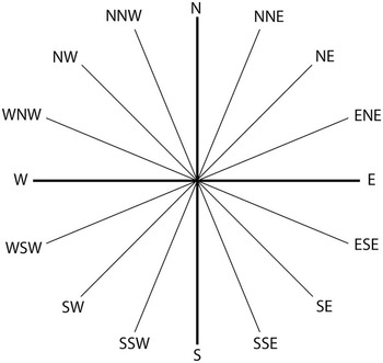
06    29   9:40 am  2.6  2.3  10.0 SE      1.3  3.7 W      SWELL     4.8

Here, the first two columns give the month and date. The third column is Eastern Daylight Time. Depending on the time of the year, it could be the Eastern Standard Time. The time zone may also be different, depending on the location of the buoy. A commonly accepted practice, however, is to use the world time (UTC, or previously GMT), but for some reason, this specific station used the Eastern time.

The next column is the significant wave height (WVHT): the average height in feet of the highest one-third of the waves during the one-hour sampling period. The fifth column is the swell height (SwH) in feet. It is the average of the highest one-third of the swells. It may be estimated as a function of wave periods or frequencies. Swell waves are waves with longer wavelength and period (compared to wind-waves) propagated into the region and not generated by local wind. The sixth column is the swell period (SwP) – the peak period in seconds. If more than one swell is present, this is the period of the swell containing the maximum energy. The seventh column is the swell direction (SwD), which is the direction from which the swells are coming. The direction is given (Fig. 1.2) on a 16-direction compass scale or 16-point compass scale, i.e. the North (N), North-Northeast (NNE), Northeast (NE), East-Northeast (ENE), East (E), East-Southeast (ESE), Southeast (SE), South-Southeast (SSE), South (S), South-Southwest (SSW), South-West (SW), West-Southwest (WSW), West (W), West-Northwest (WNW), Northwest (NW), and North-Northwest (NNW). Sometimes, the direction of winds or waves can be presented with an 8-point compass scale or 32-point compass scale. They can also be presented with digital values. The eighth column is the wind-wave height (WWH), which is the average height of the highest one-third of the wind-waves. Wind-waves are those waves generated by the local wind. The ninth column is the wind-wave period (WWP), which is the peak period in seconds of the wind-waves. The tenth column is the wind-wave direction (WWD), which is the direction from which the wind-waves are coming. Likewise, the direction is given on a 16-direction compass scale. The eleventh column is the steepness of the waves with just a few scales: very steep, steep, average, or swell. The last column is the dominant wave period (AVP) in seconds – the period with maximum energy, which is either the swell period or the wind-wave period.

Figure 1.2 The 16-point compass scale for wind and wave.

1.3.7 Rotation of Coordinate System for Wind or Current Vectors

Sometimes we need to rotate a coordinate system, in which vectors will be expressed with different coordinates. For example, we may need to compute the along shelf and across shelf wind velocity or ocean current velocity components on a continental shelf, or along-channel and across channel flow velocity components at a tidal inlet. A simple transformation performed by a rotation of the coordinate system can accomplish this.

Assume that vector $\overrightarrow{OP}$ has coordinates $(x,y)$ in the original coordinate system. The coordinate system is then rotated by an angle of $\theta$. The coordinates of point $P$ are $\left(x^{\prime },y^{\prime }\right)$ in the new system. There is a relationship between $(x,y)$ and $\left(x^{\prime },y^{\prime }\right)$, as shown below (Fig. 1.3):

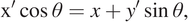$x^{\prime }\cos \theta =x+y^{\prime }\sin \theta ,$(1.7)

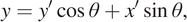$y=y^{\prime }\cos \theta +x^{\prime }\sin \theta ,$(1.8)

which lead to

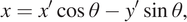$x=x^{\prime }\cos \theta -y^{\prime }\sin \theta ,$(1.9)

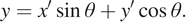$y=x^{\prime }\sin \theta +y^{\prime }\cos \theta .$(1.10)

This is a mathematical transform between the coordinates of the two systems. The inverse transform is

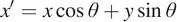$x^{\prime }=x\cos \theta +y\sin \theta$(1.11)

$y^{\prime }=-x\sin \theta +y\cos \theta .$(1.12)

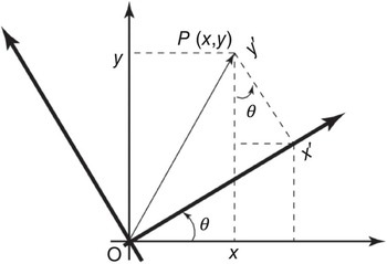
Figure 1.3 Coordinate system rotation and variable transform.

Review Questions for Chapter 1

(1) Can any real observational data be a continuous function of time?

(2) How can one determine if an observed time series contains a “jump”?

(3) Does it matter if a time series is ordered in time?

(4) What is calculus? What does it do? Why calculus is important?

(5) For time series data, do they have to be equally spaced in time (or have constant time intervals)?

(6) Contrast time series and data distributed in space (“space series”). Are there any differences or similarities?

(7) Assume that a collection of hourly time series data for wind has been obtained for a length of 1 year from Station 1. The time interval is generally 1 hour with some gaps. If the data have a few randomly distributed 2-hour gaps, 5-hour gaps, 8-hour gaps, 1-day gaps, and 3-day gaps, would you be comfortable using the data? Further assume that there is a station (Station 2) 30 km away with data from the same period but also with similar gaps. As the gaps are randomly distributed, the gaps from Station 2 are generally not the same as those from Station 1. You may want to do interpolations to fill the (short) gaps and, alternatively, use the data from Station 2 to fill the (longer) gaps as a last resort. For obvious reasons, you want to minimize the use of Station 2 data. Make a decision about how you would like to fill the data gaps (which gaps to fill with interpolations and which with replacement data from Station 2) and provide your reasoning.

(8) Wind direction is defined as the direction from which the wind comes relative to true north, measured clockwise. When wind direction is measured, however, it is often first measured relative to magnetic north. What do you think one should do to convert the wind direction to that relative to true north?

(9) Current velocity and wind velocity measurements often rely on an electronic magnetic sensor (or electronic compass) which senses the Earth’s magnetic field and determines the magnetic north. The installation of an electronic compass requires that it is away from powerlines, steel, or magnets. Why?

Exercises for Chapter 1

(1) If the wind direction were measured counterclockwise, with everything else being the same, how would you modify the equations for the east and north component of the wind velocity?

(2) If the 0 wind direction were defined from the east and measured clockwise, how would you modify the equations for the east and north component of the wind velocity?

(3) If the 0 wind direction were defined from the east and measured counterclockwise, how would you modify the equations for the east and north components of the wind velocity?