


1. Introduction
In recent years, extensive research has been carried out to explore alternative divertor configurations (ADCs) to the single-null (SN) configuration considered for ITER, where high core plasma performance can be maintained while ensuring that heat flux levels at the targets remain within material constraints (Soukhanovskii et al. Reference Soukhanovskii2013; Reimerdes et al. Reference Reimerdes2020; Militello et al. Reference Militello2021). Among various ADCs, the double-null (DN) configuration is particularly interesting (Brunner et al. Reference Brunner, Kuang, LaBombard and Terry2018; Wenninger et al. Reference Wenninger2018). For instance, the presence of two X-points enables power control through two radiation fronts. Furthermore, DN configurations facilitate easier access to the H-mode (Meyer et al. Reference Meyer2005) and allow for the safe installation of external heating systems on the quiescent high-field side (HFS) region due to its magnetic disconnection from the turbulent low-field side (LFS) (Smick, LaBombard & Hutchinson Reference Smick, LaBombard and Hutchinson2013; LaBombard et al. Reference LaBombard2017).
Double-null configurations can be combined with operation in negative triangularity (NT) scenarios (Kikuchi et al. Reference Kikuchi2015), which have recently emerged as a promising alternative to the H-mode operation in positive triangularity (PT) (Kikuchi et al. Reference Kikuchi2015). Experimental observations from various tokamaks have shown that NT L-mode plasmas can achieve H-mode-like confinement due to the reduced turbulence (Austin et al. Reference Austin2019; Coda et al. Reference Coda2021) with intrinsic edge-localized-mode-free scenarios (Austin et al. Reference Austin2019; Marinoni et al. Reference Marinoni2019; Coda et al. Reference Coda2021; Happel et al. Reference Happel, Pütterich, Told, Dunne, Fischer, Hobirk, McDermott, Plank and the2023). Moreover, recent numerical studies, including gyrokinetic (Balestri et al. Reference Balestri2024; Giannatale et al. Reference Giannatale, Bottino, Brunner, Murugappan and Villard2024; Mariani et al. Reference Mariani2024; Marinoni et al. Reference Marinoni, Austin, Candy, Chrystal, Haskey, Porkolab, Rost and Scotti2024) and fluid modelling (Riva et al. Reference Riva2017; Lim et al. Reference Lim, Giacomin, Ricci, Coelho, Février, Mancini, Silvagni and Stenger2023; Muscente et al. Reference Muscente, Innocente, Ball and Gorno2023; Tonello et al. Reference Tonello2024), provide evidence of reduced plasma turbulence when NT is considered. These findings underscore the viability of NT plasmas as an effective solution for power handling in fusion devices compared with PT H-mode plasmas.
In this work, we investigate the effects of triangularity on the scape-off layer (SOL) plasma turbulence in DN L-mode plasmas. We first observe that the decrease of the bad curvature area and the associated reduction of the interchange drive induce a reduction of SOL plasma turbulence in NT plasmas. Second, we compare the characteristic pressure length scale $L_p$
between NT and PT plasmas, and find that NT plasmas exhibit a reduced
$L_p$
between NT and PT plasmas, and find that NT plasmas exhibit a reduced $L_p$
, consistent with their lower turbulence levels. Third, a comparison of the up–down power-sharing asymmetry between the predictive scaling law derived in Lim et al. (Reference Lim, Ricci, Stenger, Lucca, Durr-Legoupil-Nicoud, Février, Theiler and Verhaegh2024) and numerical measurement demonstrates that NT–DN plasmas exhibit less up–down asymmetry, mainly due to the combined effects of a non-negligible inner heat flux and a reduced heat flux crossing the separatrix. Finally, we perform a three-dimensional analysis of the blob dynamics using a blob detection and tracking technique, comparing the behaviour of blobs in NT and PT plasmas. In particular, we derive a theoretical scaling law for blob size and velocity that includes the effects of plasma shaping, and find that NT plasmas are characterised by smaller blob sizes and slower propagation velocities, in qualitative agreement with the numerical observations. Ultimately, our analysis enables us to assess the potential advantages of NT plasmas in DN configuration for power handling.
$L_p$
, consistent with their lower turbulence levels. Third, a comparison of the up–down power-sharing asymmetry between the predictive scaling law derived in Lim et al. (Reference Lim, Ricci, Stenger, Lucca, Durr-Legoupil-Nicoud, Février, Theiler and Verhaegh2024) and numerical measurement demonstrates that NT–DN plasmas exhibit less up–down asymmetry, mainly due to the combined effects of a non-negligible inner heat flux and a reduced heat flux crossing the separatrix. Finally, we perform a three-dimensional analysis of the blob dynamics using a blob detection and tracking technique, comparing the behaviour of blobs in NT and PT plasmas. In particular, we derive a theoretical scaling law for blob size and velocity that includes the effects of plasma shaping, and find that NT plasmas are characterised by smaller blob sizes and slower propagation velocities, in qualitative agreement with the numerical observations. Ultimately, our analysis enables us to assess the potential advantages of NT plasmas in DN configuration for power handling.
In the present study, we leverage previous turbulent simulations in DN scenarios (Lim et al. Reference Lim, Ricci, Stenger, Lucca, Durr-Legoupil-Nicoud, Février, Theiler and Verhaegh2024) performed using the GBS code. These simulations identified that the power-sharing asymmetry between upper and lower outer targets is determined by the interplay between poloidal diamagnetic drifts, which enhance the asymmetry, and radial turbulent transport, which tends to reduce it, in both balanced and unbalanced DN configurations. We expand this analysis by examining the effects of triangularity on SOL plasma turbulence in DN L-mode plasmas, varying plasma resistivity, heating power and triangularity.
The structure of the present paper is as follows. Section 2 introduces the GBS model, while § 3 describes the numerical set-up parameters and the magnetic equilibria used for NT and PT plasma simulations in DN configurations. Section 4 presents the numerical results, highlighting the reduction of SOL plasma turbulence and comparing analytical estimates for the pressure gradient length with nonlinear GBS simulations. Section 5 discusses the inner–outer and upper–lower power asymmetry at the DN targets between NT and PT plasmas. Section 6 focuses on the blob analysis, illustrating the differences between NT and PT plasmas, and derives an analytical scaling law for blob size and velocity that accounts for plasma shaping effects. Finally, § 7 summarises the conclusions.
2. Numerical model
The investigations presented in this work are based on the three-dimensional drift-reduced Braginskii equations (Zeiler et al. Reference Zeiler1997) implemented in the GBS code (Ricci et al. Reference Ricci, Halpern, Jolliet, Loizu, Mosetto, Fasoli, Furno and Theiler2012; Giacomin et al. Reference Giacomin2022). GBS uses a coordinate system independent of the magnetic field, allowing for the study of various magnetic configurations, such as the snowflake (Giacomin, Stenger & Ricci Reference Giacomin, Stenger and Ricci2020), NT (Riva et al. Reference Riva2017; Lim et al. Reference Lim, Giacomin, Ricci, Coelho, Février, Mancini, Silvagni and Stenger2023), DN (Beadle & Ricci Reference Beadle and Ricci2020; Lim et al. Reference Lim, Ricci, Stenger, Lucca, Durr-Legoupil-Nicoud, Février, Theiler and Verhaegh2024) and non-axisymmetric (Coelho et al. Reference Coelho, Loizu, Ricci and Giacomin2022) configurations. It is therefore an ideal tool for investigating the effects of plasma shaping on turbulence.
In the present study, we focus on an axisymmetric magnetic field in the electrostatic limit without including the interaction between plasma and neutrals, although these are implemented in GBS (Giacomin et al. Reference Giacomin2022). As a result, the GBS model equations can be reformulated as follows:
 \begin{align} \frac {\partial n}{\partial t} = -\frac {\rho _*^{-1}}{B}[\phi , n] + \frac {2}{B}[C(p_e)-nC(\phi)]-\boldsymbol{\nabla} _\parallel (nv_{\parallel e}) + D_n {\nabla} ^2_\perp n + s_n, \end{align}
 \begin{align} \frac {\partial \varOmega }{\partial t} &= -\frac {\rho _*^{-1}}{B} \boldsymbol{\nabla }\boldsymbol{\cdot }[\phi , \omega ] -\boldsymbol{\nabla }\boldsymbol{\cdot }\big (v_{\parallel i} \boldsymbol{\nabla} _\parallel \omega \big ) + B^2 \boldsymbol{\nabla} _\parallel j_\parallel + 2B C(p_e + \tau p_i) + \frac {B}{3}C(G_i)\nonumber \\&\quad + D_\varOmega {\nabla} _\perp ^2 \varOmega , \end{align}
 \begin{align} \frac {\partial v_{\parallel i}}{\partial t} = -\frac {\rho _*^{-1}}{B}[\phi , v_{\parallel i}]-v_{\parallel i} \boldsymbol{\nabla} _\parallel v_{\parallel i} - \frac {1}{n}\boldsymbol{\nabla} _\parallel (p_e + \tau p_i) -\frac {2}{3n}\boldsymbol{\nabla} _\parallel G_i + D_{v_{\parallel i}}{\nabla} _\perp ^2 v_{\parallel i}, \end{align}
 \begin{align} \frac {\partial v_{\parallel e}}{\partial t} &= -\frac {\rho _*^{-1}}{B}[\phi , v_{\parallel , e}] - v_{\parallel e}\boldsymbol{\nabla} _\parallel v_{\parallel e} + \frac {m_i}{m_e}\!\Bigg (\!\nu j_\parallel + \boldsymbol{\nabla} _\parallel \phi -\frac {1}{n}\boldsymbol{\nabla} _\parallel p_e-0.71 \boldsymbol{\nabla} _\parallel T_e -\frac {2}{3n}\boldsymbol{\nabla} _\parallel G_e \!\Bigg ) \nonumber \\ & \quad + D_{v_{\parallel e}}{\nabla} _\perp ^2 v_{\parallel e}, \end{align}
 \begin{align} \frac {\partial T_i}{\partial t} &=-\frac {\rho _*^{-1}}{B}[\phi , T_i] - v_{\parallel i}\boldsymbol{\nabla} _\parallel T_i + \frac {4}{3}\frac {T_i}{B}\Bigg [C(T_e) + \frac {T_e}{n}C(n)-C(\phi ) \Bigg ] -\frac {10}{3}\tau \frac {T_i}{B}C(T_i) \nonumber \\ &\quad + \frac {2}{3}T_i\Bigg [(v_{\parallel i}-v_{\parallel e})\frac {\boldsymbol{\nabla} _\parallel n}{n}-T_i \boldsymbol{\nabla} _\parallel v_{\parallel e}\Bigg ] + 2.61\nu n (T_e -\tau T_i)+ \boldsymbol{\nabla} _\parallel ( \chi _{\parallel i}\boldsymbol{\nabla} _\parallel T_i) \nonumber \\ &\quad + D_{T_i}{\nabla} _\perp ^2 T_i + s_{T_i}, \end{align}
 \begin{align} \frac {\partial T_e}{\partial t} &= -\frac {\rho _*^{-1}}{B}[\phi , T_e] - v_{\parallel e}\boldsymbol{\nabla} _\parallel T_e + \frac {2}{3}T_e\Bigg [0.71 \frac {\boldsymbol{\nabla} _\parallel j_\parallel }{n}-\boldsymbol{\nabla} _\parallel v_{\parallel e}\Bigg ] -2.61\nu n (T_e-\tau T_i) \nonumber \\ &\quad+ \frac {4}{3}\frac {T_e}{B}\Bigg [\frac {7}{2}C(T_e)+\frac {T_e}{n}C(n)-C(\phi ) \Bigg ] + \boldsymbol{\nabla} _\parallel (\chi _{\parallel e}\boldsymbol{\nabla} _\parallel T_e) + D_{T_e}{\nabla} _\perp ^2 T_e + s_{T_e}. \end{align}
Here $p_{e,i}=nT_{e,i}$
are the electron and ion pressures,
$p_{e,i}=nT_{e,i}$
are the electron and ion pressures, $D_f\nabla_\perp f^2$
denotes the artificial diffusion terms,
$D_f\nabla_\perp f^2$
denotes the artificial diffusion terms, $G_e$
and
$G_e$
and $G_i$
are the gyroviscous terms, and
$G_i$
are the gyroviscous terms, and $s_n, s_{T_{i}}$
and
$s_n, s_{T_{i}}$
and $s_{T_e}$
are prescribed particle and heat source terms.
$s_{T_e}$
are prescribed particle and heat source terms.
The above equations are coupled with the Poisson equation, which avoids the Boussinesq approximation
 \begin{align} \boldsymbol{\nabla }\boldsymbol{\cdot }(n\boldsymbol{\nabla} _\perp \phi) = \varOmega - \tau {\nabla} _\perp ^2 p_i, \end{align}
where $\varOmega =\boldsymbol{\nabla }\boldsymbol{\cdot }\omega$
is the scalar vorticity, with the polarization vector
$\varOmega =\boldsymbol{\nabla }\boldsymbol{\cdot }\omega$
is the scalar vorticity, with the polarization vector $\omega=n\nabla_\perp \phi + \tau \nabla_\perp p_i$
.
$\omega=n\nabla_\perp \phi + \tau \nabla_\perp p_i$
.
In (2.1)–(2.7), the plasma variables are normalised with respect to the reference values at the separatrix. Specifically, the plasma density, $n$
, the ion and electron temperatures,
$n$
, the ion and electron temperatures, $T_i$
and
$T_i$
and $T_e$
, the ion and electron parallel velocities,
$T_e$
, the ion and electron parallel velocities, $v_{\parallel i}$
and
$v_{\parallel i}$
and $v_{\parallel e}$
, and the electric potential,
$v_{\parallel e}$
, and the electric potential, $\phi$
, are normalised to
$\phi$
, are normalised to $n_0$
,
$n_0$
, $T_{i0}$
,
$T_{i0}$
, $T_{e0}$
,
$T_{e0}$
, $c_{s0}=\sqrt {T_{e0}/m_i}$
and
$c_{s0}=\sqrt {T_{e0}/m_i}$
and $T_{e0}/e$
, respectively, where
$T_{e0}/e$
, respectively, where $m_i$
is the ion mass and
$m_i$
is the ion mass and $e$
is the elemantary charge. Perpendicular lengths are normalised to the ion sound Larmor radius
$e$
is the elemantary charge. Perpendicular lengths are normalised to the ion sound Larmor radius $\rho _{s0}=c_{s0}/\varOmega _{ci}$
, where
$\rho _{s0}=c_{s0}/\varOmega _{ci}$
, where $\varOmega _{ci}=eB/m_i$
is the ion cyclotron frequency and
$\varOmega _{ci}=eB/m_i$
is the ion cyclotron frequency and $B$
is the magnetic-field strength. Parallel lengths are normalised to the tokamak major radius,
$B$
is the magnetic-field strength. Parallel lengths are normalised to the tokamak major radius, $R_0$
. Time is normalised to
$R_0$
. Time is normalised to $R_0/c_{s0}$
.
$R_0/c_{s0}$
.
The dimensionless parameters that govern the plasma dynamics in (2.1)–(2.7) include the normalised ion Larmor radius $\rho _*=\rho _{s0}/R_0$
, the ratio of ion to electron temperature
$\rho _*=\rho _{s0}/R_0$
, the ratio of ion to electron temperature $\tau =T_{i0}/T_{e0}$
and the normalised ion and electron viscosities
$\tau =T_{i0}/T_{e0}$
and the normalised ion and electron viscosities $\eta _{0i}=0.96 n T_i \tau _i$
and
$\eta _{0i}=0.96 n T_i \tau _i$
and $\eta _{0e}=0.73 n T_e \tau _e$
, respectively, where
$\eta _{0e}=0.73 n T_e \tau _e$
, respectively, where $\tau _{e,i}$
represent the electron and ion collision times. The normalised ion and electron parallel thermal conductivities are defined as
$\tau _{e,i}$
represent the electron and ion collision times. The normalised ion and electron parallel thermal conductivities are defined as
 \begin{align} \chi _{\parallel i} = \bigg (\frac {1.94}{\sqrt {2\pi }}\sqrt {m_i} \frac {(4\pi \epsilon _0)^2}{e^4} \frac {c_{s0}}{R_0}\frac {T_{e0}^{3/2}\tau ^{5/2}}{\varLambda _c n_0} \bigg ) T_i^{5/2} \end{align}
and
 \begin{align} \chi _{\parallel e} = \bigg (\frac {1.58}{\sqrt {2\pi }}\frac {m_i}{\sqrt {m_e}}\frac {(4\pi \epsilon _0)^2}{e^4} \frac {c_{s0}}{R_0}\frac {T_{e0}^{3/2}}{\varLambda _c n_0} \bigg ) T_e^{5/2}, \end{align}
where $\epsilon_0$
is the vacuum permittivity.
$\epsilon_0$
is the vacuum permittivity.
The normalised Spitzer resistivity is defined as $\nu =e^2n_0R_0/(m_ic_{s0}\sigma _\parallel )=\nu _0 T_e^{-3/2}$
, with
$\nu =e^2n_0R_0/(m_ic_{s0}\sigma _\parallel )=\nu _0 T_e^{-3/2}$
, with
 \begin{align} \sigma _\parallel = \Bigg (1.96\frac {n_0 e^2 \tau _e}{m_e}\Bigg )n = \Bigg (\frac {5.88}{4\sqrt {2\pi }} \frac {(4\pi \epsilon _0)^2}{e^2}\frac {T_{e0}^{3/2}}{\varLambda _c \sqrt {m_e}}\Bigg )T_e^{3/2}, \end{align}
and
 \begin{align} \nu _0 =\frac {4\sqrt {2\pi }}{5.88} \frac {e^4}{(4\pi \epsilon _0)^2}\frac {\sqrt {m_e}R_0 n_0 \varLambda _c}{m_i c_{s0}T_{e0}^{3/2}}, \end{align}
where $\varLambda _c$
is the Coulomb logarithm.
$\varLambda _c$
is the Coulomb logarithm.
The differential geometrical operators used in (2.1)–(2.7) are defined as follows:
 \begin{align} [\phi ,f] &= \boldsymbol{b} \boldsymbol{\cdot }(\boldsymbol{\nabla }\phi \times \boldsymbol{\nabla }f), \end{align}
 \begin{align} \mathcal{C}(f) &= \frac {B}{2}\bigg ( \boldsymbol{\nabla }\times \frac {\boldsymbol{b}}{B}\bigg ) \boldsymbol{\cdot }\boldsymbol{\nabla }f, \end{align}
 \begin{align} \boldsymbol{\nabla} _\parallel f &= \boldsymbol{b} \boldsymbol{\cdot }\boldsymbol{\nabla }f, \end{align}
 \begin{align} {\nabla} _\perp ^2 f &=\boldsymbol{\nabla }\boldsymbol{\cdot }\big [(\boldsymbol{b}\times \boldsymbol{\nabla }f)\times \boldsymbol{b}\big ]. \end{align}
These correspond to the $E \times B$
convective term, where
$E \times B$
convective term, where $\boldsymbol{E}=-\boldsymbol{\nabla} \phi$
is the electric field, the curvature operator, the parallel gradient and the perpendicular Laplacian of a scalar function
$\boldsymbol{E}=-\boldsymbol{\nabla} \phi$
is the electric field, the curvature operator, the parallel gradient and the perpendicular Laplacian of a scalar function $f$
. To compute these differential operators, the non-field-aligned cylindrical coordinates
$f$
. To compute these differential operators, the non-field-aligned cylindrical coordinates $(R, \varphi , Z)$
are used, where
$(R, \varphi , Z)$
are used, where $R$
represents the radial distance from the torus axis of symmetry,
$R$
represents the radial distance from the torus axis of symmetry, $Z$
the vertical coordinate and
$Z$
the vertical coordinate and $\varphi$
the toroidal angle. An axisymmetric magnetic field is considered, expressed as
$\varphi$
the toroidal angle. An axisymmetric magnetic field is considered, expressed as $\boldsymbol{B}=RB_\varphi \boldsymbol{\nabla }\varphi + \boldsymbol{\nabla }\varphi \times \boldsymbol{\nabla }\psi$
, where
$\boldsymbol{B}=RB_\varphi \boldsymbol{\nabla }\varphi + \boldsymbol{\nabla }\varphi \times \boldsymbol{\nabla }\psi$
, where $\psi (R,Z)$
is the poloidal magnetic flux. Note that these operators depend on the sign of the normalised magnetic field
$\psi (R,Z)$
is the poloidal magnetic flux. Note that these operators depend on the sign of the normalised magnetic field $\boldsymbol{b}=\boldsymbol{B}/B$
, which determines whether the magnetic drifts are directed toward the lower X-point (favourable direction) or away from it (unfavourable).
$\boldsymbol{b}=\boldsymbol{B}/B$
, which determines whether the magnetic drifts are directed toward the lower X-point (favourable direction) or away from it (unfavourable).
The gyroviscous terms are defined as
 \begin{eqnarray} G_i=-\eta _{0i}\Bigg [2\boldsymbol{\nabla} _\parallel v_{\parallel i} + \frac {1}{B}C(\phi ) + \frac {1}{enB}C(p_i) \Bigg ], \end{eqnarray}
and
 \begin{eqnarray} G_e=-\eta _{0e}\Bigg [2\boldsymbol{\nabla} _\parallel v_{\parallel e} + \frac {1}{B}C(\phi )-\frac {1}{enB}C(p_e) \Bigg ]. \end{eqnarray}
To improve the numerical stability of the simulation, artificial diffusion terms $D_f{\boldsymbol{\nabla}} _\perp ^2 f$
are introduced on the right-hand sides of (2.1)–(2.7).
$D_f{\boldsymbol{\nabla}} _\perp ^2 f$
are introduced on the right-hand sides of (2.1)–(2.7).
To mimic the ionisation process and ohmic heating within the core, toroidally uniform density and temperature sources are applied inside the last closed flux surface (LCFS). These sources are expressed as follows:
 \begin{align} s_n &= s_{n0}\exp {\Bigg [ -\frac {(\psi (R,Z)-\psi _n)^2}{\varDelta _n^2}\Bigg ]}, \end{align}
 \begin{align} s_T &= \frac {s_{T0}}{2}\Bigg [\tanh \Bigg (-\frac {\psi (R,Z)-\psi _T}{\varDelta _T}\Bigg )+1\Bigg ], \end{align}
where $\psi _n$
and
$\psi _n$
and $\psi _T$
represent the flux function values inside the LCFS, determining the radial position of the sources terms, while
$\psi _T$
represent the flux function values inside the LCFS, determining the radial position of the sources terms, while $\varDelta _n$
and
$\varDelta _n$
and $\varDelta _T$
set their radial widths.
$\varDelta _T$
set their radial widths.
Boundary conditions that satisfy the Bohm–Chodura criterion are implemented at the magnetic pre-sheath entrance (Loizu et al. Reference Loizu, Ricci, Halpern and Jolliet2012). By neglecting the gradients of density and electrostatic potential in directions tangent to the wall, these boundary conditions take the following form:
 \begin{align} v_{\parallel i}&=\pm \sqrt {T_e+\tau T_i}, \end{align}
 \begin{align} v_{\parallel e}&=\pm \sqrt {T_e + \tau T_i}\exp {\Bigg ( \xi - \frac {\phi }{T_e}\Bigg )}, \end{align}
 \begin{align} \partial _Z n &= \mp \frac {n}{\sqrt {T_e+\tau T_i}}\partial _Z v_{\parallel i}, \end{align}
 \begin{align} \partial _Z \phi &= \mp \frac {T_e}{\sqrt {T_e + \tau T_i}}\partial _Z v_{\parallel i}, \end{align}
 \begin{align} \partial _Z T_e &= \partial _Z T_i = 0, \end{align}
 \begin{align} \omega &= -\frac {T_e}{T_e + \tau T_i}\big[(\partial _Z v_{\parallel i})^2 \pm \sqrt {T_e + \tau T_i} \partial ^2_Z v_{\parallel i}\big]. \end{align}
In these equations, the $\pm$
sign indicates whether the magnetic field line enters (top sign) or leaves (bottom sign) the wall, and
$\pm$
sign indicates whether the magnetic field line enters (top sign) or leaves (bottom sign) the wall, and $\xi = \log \sqrt {m_i/(2\pi m_e)}\simeq 3$
. For the left and right domain boundaries, the electric potential is defined as
$\xi = \log \sqrt {m_i/(2\pi m_e)}\simeq 3$
. For the left and right domain boundaries, the electric potential is defined as $\phi =\xi T_e$
, and the derivatives normal to the wall are set to vanish for all other quantities.
$\phi =\xi T_e$
, and the derivatives normal to the wall are set to vanish for all other quantities.
3. Simulation set-up
The poloidal magnetic flux, $\psi (R,Z)$
, is evaluated assuming a Gaussian-like current centred at the magnetic axis, along with additional current-carrying wires (C1–C8) positioned outside the simulation box (see figure 1). While the position of these coils remains fixed throughout this study, the coil currents are adjusted to achieve different values of triangularity, while maintaining a constant elongation. We note that the positions of the magnetic axis in NT and PT plasmas are chosen to prevent the strike points from falling too close to the corner of the simulation box, which could introduce numerical artefacts. Therefore, they are not consistent with the Shafranov shift.
$\psi (R,Z)$
, is evaluated assuming a Gaussian-like current centred at the magnetic axis, along with additional current-carrying wires (C1–C8) positioned outside the simulation box (see figure 1). While the position of these coils remains fixed throughout this study, the coil currents are adjusted to achieve different values of triangularity, while maintaining a constant elongation. We note that the positions of the magnetic axis in NT and PT plasmas are chosen to prevent the strike points from falling too close to the corner of the simulation box, which could introduce numerical artefacts. Therefore, they are not consistent with the Shafranov shift.
For all GBS simulations presented in this study, we adopt a parameter set-up for DN configurations similar to that described in Lim et al. (Reference Lim, Ricci, Stenger, Lucca, Durr-Legoupil-Nicoud, Février, Theiler and Verhaegh2024). Specifically, we consider a numerical grid defined by $(N_R, N_Z, N_\varphi )=(240,320, 80)$
for a simulation with domain size
$(N_R, N_Z, N_\varphi )=(240,320, 80)$
for a simulation with domain size $(L_R, L_Z)=(600\rho _{s0}, 800\rho _{s0})$
and a time step of
$(L_R, L_Z)=(600\rho _{s0}, 800\rho _{s0})$
and a time step of $\Delta t=10^{-5}R_0/c_{s0}$
. We use
$\Delta t=10^{-5}R_0/c_{s0}$
. We use $\rho _*=\rho _{s0}/R_0=1/700$
, corresponding to approximately one third the size of the Tokamak à Configuration Variable (TCV) tokamak (Reimerdes et al. Reference Reimerdes2022). The radial width and position of the source terms are set to (
$\rho _*=\rho _{s0}/R_0=1/700$
, corresponding to approximately one third the size of the Tokamak à Configuration Variable (TCV) tokamak (Reimerdes et al. Reference Reimerdes2022). The radial width and position of the source terms are set to ( $\varDelta _n, \varDelta _T) = (500, 700)$
and
$\varDelta _n, \varDelta _T) = (500, 700)$
and $(\psi _n, \psi _T)=(140, 160)$
in (2.18)–(2.19), as illustrated in the shaded region of figure 1. The heating source amplitude,
$(\psi _n, \psi _T)=(140, 160)$
in (2.18)–(2.19), as illustrated in the shaded region of figure 1. The heating source amplitude, $s_{T0}$
, is applied equally to both ion and electron species.
$s_{T0}$
, is applied equally to both ion and electron species.

Figure 1. Examples of magnetic equilibria of NT and PT plasmas in DN configurations used for the nonlinear GBS simulations. The black crosses mark the positions of the current-carrying coils (C1–C8) used to generate different values of $\delta$
. The red solid line represents the separatrix. The red shaded region indicates the area where the heating source is applied and, similarly, the green shaded region represents the density source, mimicking the ionisation processes occurring inside the separatrix. The magnetic axis positions are adjusted to prevent the divertor targets from lying at the simulation box corner, which could cause numerical artefacts.
$\delta$
. The red solid line represents the separatrix. The red shaded region indicates the area where the heating source is applied and, similarly, the green shaded region represents the density source, mimicking the ionisation processes occurring inside the separatrix. The magnetic axis positions are adjusted to prevent the divertor targets from lying at the simulation box corner, which could cause numerical artefacts.
To explore the effects of triangularity on plasma turbulence in DN configurations, we carry out a parametric scan by varying the total triangularity evaluated at the separatrix, more precisely, we consider $\delta = \{\pm 0.3, \pm 0.4, \pm 0.5\}$
, plasma resistivity
$\delta = \{\pm 0.3, \pm 0.4, \pm 0.5\}$
, plasma resistivity $\nu _0=\{0.1, 0.3, 1.0\}$
and the amplitude of heating power
$\nu _0=\{0.1, 0.3, 1.0\}$
and the amplitude of heating power $s_{T0}=\{ 0.05, 0.15, 0.3\}$
across both NT and PT plasmas, while maintaining a constant elongation
$s_{T0}=\{ 0.05, 0.15, 0.3\}$
across both NT and PT plasmas, while maintaining a constant elongation $\kappa =1.6$
. We note that, according to (2.11), a variation of the plasma resistivity is equivalent to a variation of the plasma density. To reduce the computational cost of these simulations and allow for an extensive parametric scan, we use a mass ratio of
$\kappa =1.6$
. We note that, according to (2.11), a variation of the plasma resistivity is equivalent to a variation of the plasma density. To reduce the computational cost of these simulations and allow for an extensive parametric scan, we use a mass ratio of $m_i/m_e=200$
. This reduced ion-to-electron mass ratio does not significantly affect the results of nonlinear simulations in L-mode plasmas scenarios, as plasma resistivity dominates over inertial effects when
$m_i/m_e=200$
. This reduced ion-to-electron mass ratio does not significantly affect the results of nonlinear simulations in L-mode plasmas scenarios, as plasma resistivity dominates over inertial effects when $\nu _0\gt (m_e/m_i)\gamma$
, with
$\nu _0\gt (m_e/m_i)\gamma$
, with $\gamma$
denoting the growth rate. To facilitate the analysis, we keep the plasma parameters
$\gamma$
denoting the growth rate. To facilitate the analysis, we keep the plasma parameters $\tau =T_{i0}/T_{e0}=1$
,
$\tau =T_{i0}/T_{e0}=1$
, $\eta _{0e}=\eta _{0i}=1$
and
$\eta _{0e}=\eta _{0i}=1$
and $ \chi _{\parallel e}=\chi _{\parallel i}=1$
, constant throughout our study. The safety factor is adjusted to
$ \chi _{\parallel e}=\chi _{\parallel i}=1$
, constant throughout our study. The safety factor is adjusted to $q_0 \simeq 1$
at the magnetic axis and
$q_0 \simeq 1$
at the magnetic axis and $q_{95}\simeq 4$
at the tokamak edge in both NT and PT plasmas. Additionally, the reference toroidal magnetic field
$q_{95}\simeq 4$
at the tokamak edge in both NT and PT plasmas. Additionally, the reference toroidal magnetic field $B_T$
is set for all simulations such that the ion-
$B_T$
is set for all simulations such that the ion- $\boldsymbol{\nabla }B$
drift is away from the lower X-point.
$\boldsymbol{\nabla }B$
drift is away from the lower X-point.
We use the simulation with parameters $\nu _0=0.3, s_{T0}=0.15$
and
$\nu _0=0.3, s_{T0}=0.15$
and $\delta =\pm 0.5$
as the reference case. Within the selected ranges for plasma resistivity and heating source amplitude, plasma turbulence is driven by resistive ballooning modes (RBMs) (Mosetto et al. Reference Mosetto2013; Giacomin & Ricci Reference Giacomin and Ricci2020). These modes are destabilised by the magnetic field curvature and the plasma pressure gradient (Zeiler et al. Reference Zeiler1997). The dominant RBMs in the SOL region are equivalent to those observed in tokamak L-mode operation (Fundamenski et al. Reference Fundamenski, Garcia, Naulin, Pitts, Nielsen, Rasmussen, Horacek, Graves and contributors2007; Mosetto et al. Reference Mosetto2013; Giacomin & Ricci Reference Giacomin and Ricci2020), and expected in NT plasma scenarios (Kikuchi et al. Reference Kikuchi2019).
$\delta =\pm 0.5$
as the reference case. Within the selected ranges for plasma resistivity and heating source amplitude, plasma turbulence is driven by resistive ballooning modes (RBMs) (Mosetto et al. Reference Mosetto2013; Giacomin & Ricci Reference Giacomin and Ricci2020). These modes are destabilised by the magnetic field curvature and the plasma pressure gradient (Zeiler et al. Reference Zeiler1997). The dominant RBMs in the SOL region are equivalent to those observed in tokamak L-mode operation (Fundamenski et al. Reference Fundamenski, Garcia, Naulin, Pitts, Nielsen, Rasmussen, Horacek, Graves and contributors2007; Mosetto et al. Reference Mosetto2013; Giacomin & Ricci Reference Giacomin and Ricci2020), and expected in NT plasma scenarios (Kikuchi et al. Reference Kikuchi2019).
The simulations are carried out until they reach a quasi-steady state, where the input power is balanced by perpendicular transport and losses at the vessel wall, and by averaging the plasma quantities over a time window of $10t_0$
. From now on, we denote time and toroidally averaged values with an overline and fluctuations with a tilde, such that
$10t_0$
. From now on, we denote time and toroidally averaged values with an overline and fluctuations with a tilde, such that ${f}=\bar {{f}}+\tilde {{f}}$
for a generic quantity
${f}=\bar {{f}}+\tilde {{f}}$
for a generic quantity $f$
.
$f$
.
4. Estimation of the pressure gradient length
The pressure gradient length in the near SOL, $L_{p}=-p_e/\boldsymbol{\nabla }p_e$
, is governed by the extent of SOL plasma cross-field transport and is associated with the power fall-off decay length
$L_{p}=-p_e/\boldsymbol{\nabla }p_e$
, is governed by the extent of SOL plasma cross-field transport and is associated with the power fall-off decay length $\lambda _q$
at the outer targets (Giacomin et al. Reference Giacomin2021; Lim et al. Reference Lim, Giacomin, Ricci, Coelho, Février, Mancini, Silvagni and Stenger2023). The theoretical scaling law for estimating
$\lambda _q$
at the outer targets (Giacomin et al. Reference Giacomin2021; Lim et al. Reference Lim, Giacomin, Ricci, Coelho, Février, Mancini, Silvagni and Stenger2023). The theoretical scaling law for estimating $L_p$
, which includes shaping parameters in the SN configuration, was derived in Lim et al. (Reference Lim, Giacomin, Ricci, Coelho, Février, Mancini, Silvagni and Stenger2023) and validated against DN configurations, demonstrating its applicability to both configurations (Lim et al. Reference Lim, Ricci, Stenger, Lucca, Durr-Legoupil-Nicoud, Février, Theiler and Verhaegh2024). As shown in Lim et al. (Reference Lim, Giacomin, Ricci, Coelho, Février, Mancini, Silvagni and Stenger2023), NT configurations exhibit a steeper plasma pressure profile than PT configurations due to a lower level of turbulence and associated transport.
$L_p$
, which includes shaping parameters in the SN configuration, was derived in Lim et al. (Reference Lim, Giacomin, Ricci, Coelho, Février, Mancini, Silvagni and Stenger2023) and validated against DN configurations, demonstrating its applicability to both configurations (Lim et al. Reference Lim, Ricci, Stenger, Lucca, Durr-Legoupil-Nicoud, Février, Theiler and Verhaegh2024). As shown in Lim et al. (Reference Lim, Giacomin, Ricci, Coelho, Février, Mancini, Silvagni and Stenger2023), NT configurations exhibit a steeper plasma pressure profile than PT configurations due to a lower level of turbulence and associated transport.
In this section, we compare the electron pressure, $p_e$
, obtained from nonlinear simulations, between NT and PT plasmas. In addition, we verify that SOL turbulence in the L-mode plasmas considered in the present study is mainly driven by RBMs, which is a key assumption underlying the analytical derivation of
$p_e$
, obtained from nonlinear simulations, between NT and PT plasmas. In addition, we verify that SOL turbulence in the L-mode plasmas considered in the present study is mainly driven by RBMs, which is a key assumption underlying the analytical derivation of $L_p$
. Finally, we compare the
$L_p$
. Finally, we compare the $L_p$
values derived from the analytical expression with those obtained from nonlinear simulations.
$L_p$
values derived from the analytical expression with those obtained from nonlinear simulations.

Figure 2. Equilibrium electron pressure, $p_e$
, for (a) the NT and (b) PT configurations, and snapshots of turbulent fluctuations for (c) the NT and (d) PT configurations. The reference simulations with
$p_e$
, for (a) the NT and (b) PT configurations, and snapshots of turbulent fluctuations for (c) the NT and (d) PT configurations. The reference simulations with $\nu _0=0.3$
,
$\nu _0=0.3$
, $s_{T0}=0.15$
, using
$s_{T0}=0.15$
, using $\delta =-0.5$
for (a) and (c) and
$\delta =-0.5$
for (a) and (c) and $\delta =+0.5$
for (b) and (d) are considered. Four solid lines are positioned in front of each divertor target, labelled as lower outer (LO), upper outer (UO), lower inner (LI) and upper inner (UI), where the target heat flux is evaluated.
$\delta =+0.5$
for (b) and (d) are considered. Four solid lines are positioned in front of each divertor target, labelled as lower outer (LO), upper outer (UO), lower inner (LI) and upper inner (UI), where the target heat flux is evaluated.
Figure 2 illustrates equilibrium and typical snapshots of the fluctuations of the electron pressure, $p_e$
, in NT and PT plasmas, where the wall geometry is modelled as rectangular, and the divertor targets are represented by flat plates placed at the ends of the separatrix. Similar to the SN configurations (Lim et al. Reference Lim, Giacomin, Ricci, Coelho, Février, Mancini, Silvagni and Stenger2023), NT plasmas exhibit a relatively higher equilibrium pressure,
$p_e$
, in NT and PT plasmas, where the wall geometry is modelled as rectangular, and the divertor targets are represented by flat plates placed at the ends of the separatrix. Similar to the SN configurations (Lim et al. Reference Lim, Giacomin, Ricci, Coelho, Février, Mancini, Silvagni and Stenger2023), NT plasmas exhibit a relatively higher equilibrium pressure, $\bar {p}_e$
, and reduced fluctuation levels,
$\bar {p}_e$
, and reduced fluctuation levels, $\widetilde {p}_e$
, in the SOL region compared with PT plasmas. The fluctuating components show that, in both NT and PT plasmas, turbulence develops inside the separatrix and propagates from the near to the far SOL regions due to the presence of blobs, eventually reaching the outer boundary of the simulation domain. The presence of a secondary X-point in DN configurations results in a quiescent plasma at the HFS region that is magnetically disconnected from the turbulent LFS region.
$\widetilde {p}_e$
, in the SOL region compared with PT plasmas. The fluctuating components show that, in both NT and PT plasmas, turbulence develops inside the separatrix and propagates from the near to the far SOL regions due to the presence of blobs, eventually reaching the outer boundary of the simulation domain. The presence of a secondary X-point in DN configurations results in a quiescent plasma at the HFS region that is magnetically disconnected from the turbulent LFS region.
The lower fluctuation levels in NT plasmas are associated with a reduction in interchange-driven instabilities within the bad curvature region (Lim et al. Reference Lim, Giacomin, Ricci, Coelho, Février, Mancini, Silvagni and Stenger2023). This reduction occurs mainly because particle trajectories remain longer in the bad curvature region of PT plasmas, making RBMs more susceptible to destabilisation in this region (Riva et al. Reference Riva2017). In NT plasmas, the poloidal length of the separatrix in the bad curvature region is shorter ( $\sim\! 500\rho _{s0}$
) compared with PT cases (
$\sim\! 500\rho _{s0}$
) compared with PT cases ( $\sim\! 700\rho _{s0}$
), which further suppresses the development of RBMs. The steeper pressure gradient (lower
$\sim\! 700\rho _{s0}$
), which further suppresses the development of RBMs. The steeper pressure gradient (lower $L_p$
) observed in NT plasmas results from this reduced turbulence, while the net stabilisation is governed by geometric effects such as reduced curvature drive, enhanced shear and shaping.
$L_p$
) observed in NT plasmas results from this reduced turbulence, while the net stabilisation is governed by geometric effects such as reduced curvature drive, enhanced shear and shaping.
To verify the hypothesis that RBMs dominate our L-mode plasmas and that the suppressed turbulence in NT plasmas is linked to a reduction in interchange instabilities, we remove the curvature operator in the vorticity equation, (2.2), which constitutes the RBM drive, and compare its impact on SOL plasma turbulence. Figure 3 presents two-dimensional snapshots of density fluctuations in NT and PT plasmas with and without the RBM drive. First, consistent with figure 2, PT plasmas display higher levels of density fluctuations compared with NT plasmas (figures 3(a) and 3(c)). Second, we observe a significant disappearance of the fluctuating structures in both the near and far SOL regions when the RBM drive is removed (figures 3(b) and 3(d)). This suggests that the simulations carried out in the L-mode plasma conditions considered here are dominated by RBMs, which is the primary assumption behind the analytical derivations that follow, particularly for the $L_p$
gradient length.
$L_p$
gradient length.

Figure 3. Two-dimensional snapshots of density fluctuations from the reference simulations: (a) NT with RBM drive, (b) NT without RBM drive, (c) PT with RBM drive, (d) PT without RBM drive. The curvature operator in the vorticity equation from (2.2) is zeroed out, removing the RBM drive.
The analytical derivation of $L_p$
is based on a gradient removal theory (Ricci, Rogers & Brunner Reference Ricci, Rogers and Brunner2008; Ricci & Rogers Reference Ricci and Rogers2013), where the local flattening of the plasma pressure profile provides the main mechanism for the saturation of the growth of linear instabilities that drive turbulence. The value of
$L_p$
is based on a gradient removal theory (Ricci, Rogers & Brunner Reference Ricci, Rogers and Brunner2008; Ricci & Rogers Reference Ricci and Rogers2013), where the local flattening of the plasma pressure profile provides the main mechanism for the saturation of the growth of linear instabilities that drive turbulence. The value of $L_p$
is then determined by balancing perpendicular turbulent transport with parallel losses at the divertor targets. A detailed derivation of
$L_p$
is then determined by balancing perpendicular turbulent transport with parallel losses at the divertor targets. A detailed derivation of $L_p$
can be found in Lim et al. (Reference Lim, Giacomin, Ricci, Coelho, Février, Mancini, Silvagni and Stenger2023). The analytical expression for the
$L_p$
can be found in Lim et al. (Reference Lim, Giacomin, Ricci, Coelho, Février, Mancini, Silvagni and Stenger2023). The analytical expression for the $L_p$
estimate in DN configurations, which accounts for elongation and triangularity effects, is given by
$L_p$
estimate in DN configurations, which accounts for elongation and triangularity effects, is given by
 \begin{align} L_{p} \sim \mathcal{C}(\kappa , \delta , q) \bigg [ \rho _* (\nu _0 \bar {n} q^2)^2 \bigg (\frac {L_\chi \bar {p}_e}{S_p}\bigg )^{4} \bigg ]^{1/3}, \end{align}
where $q$
is the safety factor at the tokamak edge,
$q$
is the safety factor at the tokamak edge, $L_\chi \simeq \pi a (0.45 + 0.55\kappa ) + 1.33a\delta$
is an approximation of the poloidal length of the separatrix,
$L_\chi \simeq \pi a (0.45 + 0.55\kappa ) + 1.33a\delta$
is an approximation of the poloidal length of the separatrix, $a$
is the tokamak minor radius,
$a$
is the tokamak minor radius, $\kappa$
is the plasma elongation, and
$\kappa$
is the plasma elongation, and $S_p$
represents the volume-integrated power source within the separatrix (Lim et al. Reference Lim, Giacomin, Ricci, Coelho, Février, Mancini, Silvagni and Stenger2023). The curvature operator,
$S_p$
represents the volume-integrated power source within the separatrix (Lim et al. Reference Lim, Giacomin, Ricci, Coelho, Février, Mancini, Silvagni and Stenger2023). The curvature operator, $\mathcal{C}(\kappa , \delta , q)$
, defined at the outer midplane
$\mathcal{C}(\kappa , \delta , q)$
, defined at the outer midplane $(\theta =0)$
where RBMs are mostly destabilised, is expressed as
$(\theta =0)$
where RBMs are mostly destabilised, is expressed as
 \begin{align} \mathcal{C}(\kappa , \delta , q) = 1-\frac {\kappa -1}{\kappa +1}\frac {3q}{q+2} + \frac {\delta q}{1+q} + \frac {(\kappa -1)^2(5q-2)}{2(\kappa +1)^2(q+2)} + \frac {\delta ^2}{16}\frac {7q-1}{1+q}. \end{align}
The analytical $L_p$
scaling law in (4.1) has been validated against experimental multi-machine datasets, focusing also on plasma shaping effects within SN configurations (Lim et al. Reference Lim, Giacomin, Ricci, Coelho, Février, Mancini, Silvagni and Stenger2023), demonstrating its reliability in predicting
$L_p$
scaling law in (4.1) has been validated against experimental multi-machine datasets, focusing also on plasma shaping effects within SN configurations (Lim et al. Reference Lim, Giacomin, Ricci, Coelho, Février, Mancini, Silvagni and Stenger2023), demonstrating its reliability in predicting $\lambda _q$
across both NT and PT plasmas. The
$\lambda _q$
across both NT and PT plasmas. The $L_p$
estimate was applied to DN configurations (Lim et al. Reference Lim, Ricci, Stenger, Lucca, Durr-Legoupil-Nicoud, Février, Theiler and Verhaegh2024) and will be used to estimate
$L_p$
estimate was applied to DN configurations (Lim et al. Reference Lim, Ricci, Stenger, Lucca, Durr-Legoupil-Nicoud, Février, Theiler and Verhaegh2024) and will be used to estimate $\lambda _q$
for both upper and lower outer targets.
$\lambda _q$
for both upper and lower outer targets.

Figure 4. Comparison of the pressure gradient length, $L_p$
, between the analytical scaling law in (4.1) and the nonlinear GBS simulations. A scan of plasma resistivity
$L_p$
, between the analytical scaling law in (4.1) and the nonlinear GBS simulations. A scan of plasma resistivity $\nu _0$
, heating power
$\nu _0$
, heating power $s_{T0}$
and triangularity
$s_{T0}$
and triangularity $\delta$
is carried out for both NT and PT plasmas. The
$\delta$
is carried out for both NT and PT plasmas. The $R^2$
-score of the comparison is, approximately,
$R^2$
-score of the comparison is, approximately, $0.728$
.
$0.728$
.
Figure 4 compares the analytical $L_p$
estimate derived in (4.1) with the
$L_p$
estimate derived in (4.1) with the $L_p$
values obtained from nonlinear GBS simulations. The
$L_p$
values obtained from nonlinear GBS simulations. The $L_p$
values are calculated by considering the value of
$L_p$
values are calculated by considering the value of $p_e$
at the separatrix and evaluating its gradient over a radial interval extending
$p_e$
at the separatrix and evaluating its gradient over a radial interval extending $ 40\rho _{s0}$
, centred at the separatrix. The analytical scaling law captures the
$ 40\rho _{s0}$
, centred at the separatrix. The analytical scaling law captures the $L_p$
trend with an
$L_p$
trend with an $R^2$
-score of 0.728. According to the analytical expression in (4.1),
$R^2$
-score of 0.728. According to the analytical expression in (4.1), $L_p$
increases with plasma resistivity
$L_p$
increases with plasma resistivity $\nu _0$
and decreases with input heating power
$\nu _0$
and decreases with input heating power $s_{T0}$
. This relationship aligns with previous findings that higher resistivity and lower heating power enhance turbulence fluctuations and cross-field transport (Giacomin & Ricci Reference Giacomin and Ricci2020), which flattens the pressure profile in the near SOL and results in higher
$s_{T0}$
. This relationship aligns with previous findings that higher resistivity and lower heating power enhance turbulence fluctuations and cross-field transport (Giacomin & Ricci Reference Giacomin and Ricci2020), which flattens the pressure profile in the near SOL and results in higher $L_p$
values. As shown in figure 2, reduced fluctuation levels in NT result in smaller
$L_p$
values. As shown in figure 2, reduced fluctuation levels in NT result in smaller $L_p$
and, overall,
$L_p$
and, overall, $L_p$
increases with
$L_p$
increases with $\delta$
.
$\delta$
.
5. Target heat load and in–out and up–down asymmetries
Experimental observations from various tokamaks report a pronounced in–out power load asymmetry (Liu et al. Reference Liu2014, Reference Liu2016; Du et al. Reference Du2017), as well as an up–down asymmetry (Morel, Counsell & Helander Reference Morel, Counsell and Helander1999; Petrie et al. Reference Petrie2001; De Temmerman et al. Reference De Temmerman, Kirk, Nardon and Tamain2011; Brunner et al. Reference Brunner, Kuang, LaBombard and Terry2018; Février et al. Reference Février2021). Several key mechanisms have been suggested to explain these power-sharing asymmetries, including cross-field drifts (Cohen & Ryutov Reference Cohen and Ryutov1999; Rognlien, Porter & Ryutov Reference Rognlien, Porter and Ryutov1999; Rensink et al. Reference Rensink, Allen, Porter and Rognlien2000; Rubino et al. Reference Rubino2020), ballooning modes (Du et al. Reference Du2015), Pfirsch-Schlüter flows (Schaffer et al. Reference Schaffer1997; Asakura et al. Reference Asakura2004), flux compression between the two separatrices (Osawa et al. Reference Osawa, Moulton, Newton, Henderson, Lipschultz and Hudoba2023) and variations in recycling rates at the divertor targets (Rensink et al. Reference Rensink, Allen, Porter and Rognlien2000).
Recent work with DN configurations using GBS suggests that the interplay between poloidal diamagnetic drift and radial turbulent transport is a key factor in determining the up–down power asymmetry, along with the magnetic imbalance (Lim et al. Reference Lim, Ricci, Stenger, Lucca, Durr-Legoupil-Nicoud, Février, Theiler and Verhaegh2024). More precisely, poloidal diamagnetic drift tends to increase the up–down asymmetry, while radial turbulent transport reduces it. Negative triangularity plasmas with DN configurations operating in L-mode scenarios (Kikuchi et al. Reference Kikuchi2019) exhibit stronger plasma turbulence and associated cross-field transport than H-mode discharges, which might reduce up–down power load asymmetry, a beneficial effect for the operation of a fusion power plant.
To estimate the effects of triangularity on power load distribution, we analyse the lower outer (LO) and lower inner (LI) targets, while the upper ones behave similarly by DN symmetry, as shown in figure 2. These plates are located midway between the X-point and the wall to avoid numerical artefacts near the walls. The heat flux at the upper outer (UO) and upper inner (UI) targets is evaluated similarly.

Figure 5. Percentage of the heat flux at the (a) LO and (b) LI targets for NT (blue) and PT (red) plasmas. The parallel heat flux $q_\parallel$
is time averaged over a time interval of 10
$q_\parallel$
is time averaged over a time interval of 10 $t_0$
, where
$t_0$
, where $t_0=R_0/c_{s0}$
. A scan of plasma resistivity, heating power and triangularities is considered.
$t_0=R_0/c_{s0}$
. A scan of plasma resistivity, heating power and triangularities is considered.
Figure 5 presents the time-integrated parallel heat flux reaching the LO and LI targets, for simulations carried out with different values of plasma resistivity $\nu _0$
, input heating power
$\nu _0$
, input heating power $s_{T0}$
and triangularity
$s_{T0}$
and triangularity $\delta$
. Consistent with previous results (Lim et al. Reference Lim, Ricci, Stenger, Lucca, Durr-Legoupil-Nicoud, Février, Theiler and Verhaegh2024), the magnetic disconnection between the quiescent HFS and the turbulent LFS causes less than
$\delta$
. Consistent with previous results (Lim et al. Reference Lim, Ricci, Stenger, Lucca, Durr-Legoupil-Nicoud, Février, Theiler and Verhaegh2024), the magnetic disconnection between the quiescent HFS and the turbulent LFS causes less than $90\,\%$
of the total heat flux to reach the outer targets in both NT and PT plasmas. More precisely, across all values of
$90\,\%$
of the total heat flux to reach the outer targets in both NT and PT plasmas. More precisely, across all values of $\nu _0$
and
$\nu _0$
and $s_{T0}$
, PT plasmas (red) exhibit a larger heat flux at the outer target compared with NT plasmas (blue). Indeed, PT plasmas are characterised by a negligible inner heat flux, less than 5 %, whereas NT plasmas present a more significant inner heat flux, up to 10 %. Consequently, the in–out power asymmetry decreases in NT plasmas, while it becomes more pronounced in PT plasmas.
$s_{T0}$
, PT plasmas (red) exhibit a larger heat flux at the outer target compared with NT plasmas (blue). Indeed, PT plasmas are characterised by a negligible inner heat flux, less than 5 %, whereas NT plasmas present a more significant inner heat flux, up to 10 %. Consequently, the in–out power asymmetry decreases in NT plasmas, while it becomes more pronounced in PT plasmas.
The non-negligible power load at the inner targets in NT plasmas can be attributed to both geometrical factors and cross-field turbulent transport. First, as illustrated in figure 2, the longer separatrix at the HFS in NT plasmas leads to an increased heat flux crossing the HFS separatrix. Second, the reduced levels of cross-field turbulent transport at the LFS in NT plasmas contribute to a considerable power load at the inner targets, thereby reducing in–out power asymmetry in NT plasmas. Indeed, previous studies on the EAST tokamak and BOUT++ simulations (Liu et al. Reference Liu2012, Reference Liu2014) have shown that in–out power asymmetry scales with the power crossing the separatrix, $P_{\textrm {SOL}}$
. This suggests that enhanced SOL turbulence leads to a stronger in–out power asymmetry, consistent with the behaviour observed in the PT plasmas considered in this study.
$P_{\textrm {SOL}}$
. This suggests that enhanced SOL turbulence leads to a stronger in–out power asymmetry, consistent with the behaviour observed in the PT plasmas considered in this study.
We now turn our attention to the up–down power-sharing asymmetry. We apply the predictive analytical scaling law derived in Lim et al. (Reference Lim, Ricci, Stenger, Lucca, Durr-Legoupil-Nicoud, Février, Theiler and Verhaegh2024) to evaluate the up–down asymmetry at the outer targets in DN configurations, exploring the effects of plasma triangularity. In balanced DN configurations with an inter-separatrix distance of $\delta R=0$
considered here, the scaling law proposed in Lim et al. (Reference Lim, Ricci, Stenger, Lucca, Durr-Legoupil-Nicoud, Février, Theiler and Verhaegh2024) reduces to
$\delta R=0$
considered here, the scaling law proposed in Lim et al. (Reference Lim, Ricci, Stenger, Lucca, Durr-Legoupil-Nicoud, Février, Theiler and Verhaegh2024) reduces to
 \begin{align} \lvert q_{\parallel , \textrm {LO}} - q_{\parallel , \textrm {UO}}\rvert =q_{\textrm {asym}} &= q_\psi \alpha _d K, \end{align}
with
 \begin{align} \alpha _d = \rho _*^{3/4} \bar {n}^{-3/2} \bar {p}_e L_p^{-1/4} \nu _0^{-1/2}q^{-1}, \end{align}
where $q_\psi$
is the heat flux crossing the separatrix in the LFS region,
$q_\psi$
is the heat flux crossing the separatrix in the LFS region, $\alpha _d$
is a dimensionless diamagnetic parameter that includes the effects of both diamagnetic drift and turbulence and
$\alpha _d$
is a dimensionless diamagnetic parameter that includes the effects of both diamagnetic drift and turbulence and $K$
is a numerical coefficient used to account for the order of magnitude estimates considered and determined by fitting simulations and experimental results.
$K$
is a numerical coefficient used to account for the order of magnitude estimates considered and determined by fitting simulations and experimental results.
The parameter $\alpha _d$
in (5.1) represents the competing effects of diamagnetic drift and turbulence in generating up–down heat asymmetry. Given the dominant RBM nature of turbulence in our simulations, we define
$\alpha _d$
in (5.1) represents the competing effects of diamagnetic drift and turbulence in generating up–down heat asymmetry. Given the dominant RBM nature of turbulence in our simulations, we define $\alpha _d=\lvert \boldsymbol{v}_d \rvert k_{\textrm {RBM}}/\gamma _{\textrm {RBM}}$
with
$\alpha _d=\lvert \boldsymbol{v}_d \rvert k_{\textrm {RBM}}/\gamma _{\textrm {RBM}}$
with $\boldsymbol{v}_d$
the diamagnetic velocity and the characteristic wavenumber and the growth rate of the RBMs, being defined as
$\boldsymbol{v}_d$
the diamagnetic velocity and the characteristic wavenumber and the growth rate of the RBMs, being defined as $k_{\textrm {RBM}}=1/\sqrt {\bar {n}\nu q^2 \gamma _{\textrm {RBM}}}$
and
$k_{\textrm {RBM}}=1/\sqrt {\bar {n}\nu q^2 \gamma _{\textrm {RBM}}}$
and $\gamma _{\textrm {RBM}}=\sqrt {(2\bar {T}_e)/(\rho _* L_p)}$
, respectively. We approximate
$\gamma _{\textrm {RBM}}=\sqrt {(2\bar {T}_e)/(\rho _* L_p)}$
, respectively. We approximate $\lvert \boldsymbol{v}_d \rvert \simeq \bar {p}_e/(\bar {n} L_p)$
. Higher
$\lvert \boldsymbol{v}_d \rvert \simeq \bar {p}_e/(\bar {n} L_p)$
. Higher $\alpha _d$
values indicate more pronounced asymmetry-driving mechanisms.
$\alpha _d$
values indicate more pronounced asymmetry-driving mechanisms.

Figure 6. Comparison of the heat flux asymmetry between the analytical scaling law in (5.1) and the nonlinear GBS simulations. We set $K=3.43$
for all the simulations, and obtain an
$K=3.43$
for all the simulations, and obtain an $R^2$
-score of 0.74.
$R^2$
-score of 0.74.
Figure 6 compares the heat flux asymmetry, $q_{\rm {asym}}$
, predicted by the analytical scaling law in (5.1), with the results from nonlinear GBS simulations. We set the prefactor
$q_{\rm {asym}}$
, predicted by the analytical scaling law in (5.1), with the results from nonlinear GBS simulations. We set the prefactor $K=3.43$
, determined using linear regression methods, whereas in Lim et al. (Reference Lim, Ricci, Stenger, Lucca, Durr-Legoupil-Nicoud, Février, Theiler and Verhaegh2024), the prefactor was set to
$K=3.43$
, determined using linear regression methods, whereas in Lim et al. (Reference Lim, Ricci, Stenger, Lucca, Durr-Legoupil-Nicoud, Février, Theiler and Verhaegh2024), the prefactor was set to $K = 2.84$
. The difference is due to the variation in the parameter spaces explored in these works. Overall, the scaling law effectively captures the trend of heat asymmetry observed across various simulations. Consistent with Lim et al. (Reference Lim, Ricci, Stenger, Lucca, Durr-Legoupil-Nicoud, Février, Theiler and Verhaegh2024), increasing
$K = 2.84$
. The difference is due to the variation in the parameter spaces explored in these works. Overall, the scaling law effectively captures the trend of heat asymmetry observed across various simulations. Consistent with Lim et al. (Reference Lim, Ricci, Stenger, Lucca, Durr-Legoupil-Nicoud, Février, Theiler and Verhaegh2024), increasing $\nu _0$
and decreasing
$\nu _0$
and decreasing $s_{T0}$
lead to a reduction of the up–down heat asymmetry, as a consequence of the decrease in
$s_{T0}$
lead to a reduction of the up–down heat asymmetry, as a consequence of the decrease in $\alpha _d$
of (5.1).
$\alpha _d$
of (5.1).
The clear difference in heat asymmetry between NT and PT plasmas is highlighted in figure 6, with PT plasmas showing more pronounced heat asymmetry. This behaviour is described by (5.1), where $q_{\textrm {asym}}$
is directly proportional to the heat flux crossing the separatrix in the LFS region,
$q_{\textrm {asym}}$
is directly proportional to the heat flux crossing the separatrix in the LFS region, $q_\psi$
, as well as the dimensionless diamagnetic parameter,
$q_\psi$
, as well as the dimensionless diamagnetic parameter, $\alpha _d$
. The reduced up–down heat asymmetry at the outer targets in NT plasmas can be attributed to two main factors. First, the scaling law in (5.1) does not account for inner heat loads. However, NT plasmas exhibit a non-negligible amount of inner heat load, which decreases the up–down asymmetry at the outer targets. Second, the heat flux crossing the separatrix in the LFS region is smaller in NT plasmas compared with PT plasmas, further reducing the observed up–down asymmetry. Consequently, although the smaller
$\alpha _d$
. The reduced up–down heat asymmetry at the outer targets in NT plasmas can be attributed to two main factors. First, the scaling law in (5.1) does not account for inner heat loads. However, NT plasmas exhibit a non-negligible amount of inner heat load, which decreases the up–down asymmetry at the outer targets. Second, the heat flux crossing the separatrix in the LFS region is smaller in NT plasmas compared with PT plasmas, further reducing the observed up–down asymmetry. Consequently, although the smaller $L_p$
in NT plasmas leads to a larger
$L_p$
in NT plasmas leads to a larger $\alpha _d$
, the combined effects of the inner heat load and reduced
$\alpha _d$
, the combined effects of the inner heat load and reduced $q_\psi$
eventually result in the mitigated up–down heat asymmetry at the outer targets observed in figure 6.
$q_\psi$
eventually result in the mitigated up–down heat asymmetry at the outer targets observed in figure 6.
It is important to note that the up–down asymmetry, $q_{\textrm {asym}}$
, depends on the magnetic imbalance. Achieving an ideal equal distribution between UO and LO targets in future fusion devices may therefore require proper control of the DN magnetic imbalance.
$q_{\textrm {asym}}$
, depends on the magnetic imbalance. Achieving an ideal equal distribution between UO and LO targets in future fusion devices may therefore require proper control of the DN magnetic imbalance.
6. Blob dynamics
Blobs are coherent plasma structures that originate in the edge region and move toward the far SOL (Myra et al. Reference Myra, DIppolito, Stotler, Zweben, LeBlanc, Menard, Maqueda and Boedo2006a ; Zweben et al. Reference Zweben, Boedo, Grulke, Hidalgo, LaBombard, Maqueda, Scarin and Terry2007; DIppolito, Myra & Zweben Reference DIppolito, Myra and Zweben2011). Experimental observations clearly show that blobs typically form at the outer midplane (OMP) in the LFS, where the curvature-driven interchange instabilities are present (Rudakov et al. Reference Rudakov2002; Zweben et al. Reference Zweben, Boedo, Grulke, Hidalgo, LaBombard, Maqueda, Scarin and Terry2007). This suggests a link between RBMs and blob formation, as well as the effect of triangularity on the blob dynamics.
To investigate the blob dynamics (Angus, Krasheninnikov & Umansky Reference Angus, Krasheninnikov and Umansky2012; Walkden, Dudson & Fishpool Reference Walkden, Dudson and Fishpool2013; Easy et al. Reference Easy, Militello, Omotani, Dudson, Havlíčková, Tamain, Naulin and Nielsen2014), three-dimensional simulations have been carried out using various codes, such as BOUT++ (Russell et al. Reference Russell, DIppolito, Myra, Nevins and Xu2004), GBS (Nespoli et al. Reference Nespoli, Furno, Labit, Ricci, Avino, Halpern, Musil and Riva2017; Paruta et al. Reference Paruta, Beadle, Ricci and Theiler2019) and GRILLIX (Ross et al. Reference Ross, Stegmeir, Manz, Groselj, Zholobenko, Coster and Jenko2019; Zholobenko et al. Reference Zholobenko, Pfennig, Stegmeir, Body, Ulbl and Jenko2023). Despite the extensive studies, the effect of triangularity on the blob dynamics has yet to be investigated.
In this section, we present a three-dimensional blob analysis from nonlinear GBS simulations for PT and NT plasmas. We begin by applying blob detection techniques to identify blobs, as well as their sizes and velocities. The detected blobs are then compared with the two-region model (Myra et al. Reference Myra, Russell and DIppolito2006b ) to elucidate the main mechanisms behind the blob dynamics. Finally, we derive a new analytical scaling law for blob size and radial blob velocity by including the effects of triangularity, explaining the observed trends from the nonlinear GBS simulations.
6.1. Blob detection and tracking
To detect and track the motion of blobs in the GBS simulation, we use an image processing algorithm (van der Walt et al. Reference van der Walt2014). We detect blobs as structures that meet the condition $n_{\rm {blobs}}(R, Z, t) \gt \bar {n}(R, Z) + 2.5 \sigma _n(R, Z)$
, where
$n_{\rm {blobs}}(R, Z, t) \gt \bar {n}(R, Z) + 2.5 \sigma _n(R, Z)$
, where $\sigma _n$
is the standard deviation of the density. Consistent with previous GBS works in Nespoli et al. (Reference Nespoli, Furno, Labit, Ricci, Avino, Halpern, Musil and Riva2017) and Paruta et al. (Reference Paruta, Beadle, Ricci and Theiler2019), once detected, a blob is tracked from one time frame to the next. However, in contrast to Nespoli et al. (Reference Nespoli, Furno, Labit, Ricci, Avino, Halpern, Musil and Riva2017) and Paruta et al. (Reference Paruta, Beadle, Ricci and Theiler2019) and for the sake of simplicity, we do not account for merging and splitting events.
$\sigma _n$
is the standard deviation of the density. Consistent with previous GBS works in Nespoli et al. (Reference Nespoli, Furno, Labit, Ricci, Avino, Halpern, Musil and Riva2017) and Paruta et al. (Reference Paruta, Beadle, Ricci and Theiler2019), once detected, a blob is tracked from one time frame to the next. However, in contrast to Nespoli et al. (Reference Nespoli, Furno, Labit, Ricci, Avino, Halpern, Musil and Riva2017) and Paruta et al. (Reference Paruta, Beadle, Ricci and Theiler2019) and for the sake of simplicity, we do not account for merging and splitting events.
We focus our analysis on blob size and velocity, highlighting the differences between NT and PT plasmas in DN configurations, considering only blobs located outside the separatrix, as shown by the grey-shaded region in figure 7. Blobs are approximated as circles, centred at the blob centre of mass location. The blob velocity is then determined by evaluating the distance travelled by the centre of mass during the blob analysis time window, $t_{\rm {blobs}}$
.
$t_{\rm {blobs}}$
.

Figure 7. Two-dimensional snapshot of blob detection in NT and PT plasmas. Blobs that meet the threshold condition in the LFS region outside the separatrix (grey region) are detected, with their contours outlined as solid white lines. The centre of mass of each detected blob is marked with a cyan dot.
Figure 7 shows the result of the blob detection technique on a typical snapshot of the density fluctuations in a poloidal plane. The contours of regions that meet the blob conditions defined above are highlighted, with the centre of mass of each blob identified. Figure 7 reveals that triangularity affects the blob properties. Blobs in PT plasmas are larger than those in NT plasmas and extend across the entire LFS region, reaching the divertor region. In contrast, blobs in NT plasmas are mostly localised near the OMP. This observation confirms the reduced blob transport to the first wall in NT plasmas, as experimentally observed in TCV discharges (Han et al. Reference Han2021).
The results of the blob detection methods applied over a period of $10 t_0$
are summarised in table 1, detailing the average number of blobs, their average radius and their average radial velocity. Confirming the findings in figure 7, PT plasmas exhibit larger blob sizes and higher propagation velocities compared with NT plasmas, which instead exhibiting a greater number of blobs. Blob size and propagation velocities are found to follow the intensity of background turbulence; more precisely, these quantities increase with
$10 t_0$
are summarised in table 1, detailing the average number of blobs, their average radius and their average radial velocity. Confirming the findings in figure 7, PT plasmas exhibit larger blob sizes and higher propagation velocities compared with NT plasmas, which instead exhibiting a greater number of blobs. Blob size and propagation velocities are found to follow the intensity of background turbulence; more precisely, these quantities increase with $\nu _0$
and decrease with
$\nu _0$
and decrease with $s_{T0}$
. The effect of triangularity affects the blob velocity more significantly than their size. A detailed analysis of these observations is provided below.
$s_{T0}$
. The effect of triangularity affects the blob velocity more significantly than their size. A detailed analysis of these observations is provided below.
Table 1. Blob detection results for both PT and NT plasmas with the average number of blobs, average radius and average velocity. The radius and velocity are normalised to $\rho _{s0}$
and
$\rho _{s0}$
and $c_{s0}$
, respectively.
$c_{s0}$
, respectively.

6.2. Two-region model for blob analysis
A large number of theoretical investigations have focused on the understanding of the blob dynamics (see, e.g. Krasheninnikov Reference Krasheninnikov2001, Yu & Krasheninnikov Reference Yu and Krasheninnikov2003, Aydemir Reference Aydemir2005, DIppolito et al. Reference DIppolito, Myra and Zweben2011). An estimate of the radial velocity of blobs in different regimes was first presented in Myra et al. (Reference Myra, Russell and DIppolito2006b
), providing an analogy with an electrical circuit. The regimes are identified depending on the current restoring the quasi-neutrality, which balances the magnetic curvature and gradient drift responsible for the charge separation driving the $E \times B$
radial motion. This analysis identifies four different regimes of blob motion, defined by two parameters: the normalised cross-section size
$E \times B$
radial motion. This analysis identifies four different regimes of blob motion, defined by two parameters: the normalised cross-section size $\varTheta$
, and the effective collisionality parameter
$\varTheta$
, and the effective collisionality parameter $\varLambda$
. These parameters are defined as follows:
$\varLambda$
. These parameters are defined as follows:
 \begin{align} \varTheta =\hat {a}^{5/2}, \end{align}
and
 \begin{align} \varLambda = \frac {\nu _{ei} L_1^2}{\rho _s \varOmega _{ce} L_2}. \end{align}
Here, $\nu _{ei}$
is the electron-to-ion collision frequency at the OMP,
$\nu _{ei}$
is the electron-to-ion collision frequency at the OMP, $L_1$
represents the connection length from the OMP to the X-point,
$L_1$
represents the connection length from the OMP to the X-point, $L_2$
is the connection length from the X-point to the outer target and
$L_2$
is the connection length from the X-point to the outer target and $\hat {a}$
is the normalised radial blob size defined as follows:
$\hat {a}$
is the normalised radial blob size defined as follows:
 \begin{align} \hat {a}=\frac {a_b R^{1/5}}{L_\parallel ^{2/5}\rho _s^{4/5}}, \end{align}
where $a_b$
is the blob size and
$a_b$
is the blob size and $L_\parallel$
is the parallel connection length to the outer divertor target.
$L_\parallel$
is the parallel connection length to the outer divertor target.
The four different regimes – (i) the sheath-connected regime $(C_s)$
, (ii) the connected ideal-interchange regime
$(C_s)$
, (ii) the connected ideal-interchange regime $(C_i)$
, (iii) the resistive X-point regime and (iv) the resistive ballooning (RB) regime. Each regime exhibits a distinct velocity scaling that is separated in terms of the normalised radial blob size,
$(C_i)$
, (iii) the resistive X-point regime and (iv) the resistive ballooning (RB) regime. Each regime exhibits a distinct velocity scaling that is separated in terms of the normalised radial blob size, $\hat {a}$
, defined in (6.3), and the normalised blob velocity
$\hat {a}$
, defined in (6.3), and the normalised blob velocity
 \begin{align} \hat {v}= \frac {v_R}{ ({2 L_\parallel \rho _s^2/R^3})^{1/5} c_s}, \end{align}
where $v_R$
is the radial velocity of the blobs (Aydemir Reference Aydemir2005; Yu, Krasheninnikov & Guzdar Reference Yu, Krasheninnikov and Guzdar2006).
$v_R$
is the radial velocity of the blobs (Aydemir Reference Aydemir2005; Yu, Krasheninnikov & Guzdar Reference Yu, Krasheninnikov and Guzdar2006).

Figure 8. Identification of four different regimes of the blob dynamics in the ( $\varTheta ,\varLambda$
) diagram. Individual blobs detected in the simulations are shown with semi-transparent markers in the background, while the average values are indicated by solid markers.
$\varTheta ,\varLambda$
) diagram. Individual blobs detected in the simulations are shown with semi-transparent markers in the background, while the average values are indicated by solid markers.
Figure 8 illustrates the result of the regime identification for the detected blobs in the $(\varTheta , \varLambda )$
diagram. Blobs are predominantly found in the RB regime, corresponding to L-mode plasma conditions with high plasma resistivity
$(\varTheta , \varLambda )$
diagram. Blobs are predominantly found in the RB regime, corresponding to L-mode plasma conditions with high plasma resistivity $\nu _0$
, resulting in high values of
$\nu _0$
, resulting in high values of $\varLambda$
. These observations are consistent with those in TCV experiments, where most blobs are found in the RB regime (Tsui et al. Reference Tsui2018). Increasing plasma resistivity tends to increase both
$\varLambda$
. These observations are consistent with those in TCV experiments, where most blobs are found in the RB regime (Tsui et al. Reference Tsui2018). Increasing plasma resistivity tends to increase both $\varLambda$
and
$\varLambda$
and $\varTheta$
, whereas increasing input heating power tends to decrease both, aligning with the experimental observations from the TCV tokamak (Offeddu et al. Reference Offeddu2022).
$\varTheta$
, whereas increasing input heating power tends to decrease both, aligning with the experimental observations from the TCV tokamak (Offeddu et al. Reference Offeddu2022).
The differences between NT and PT plasmas are also evident in figure 8. First, NT plasmas exhibit larger values of collisionality ( $\varLambda$
), pointing out that blobs are less connected to the sheath due to reduced parallel current closure, compared with the PT case. This is further demonstrated in figure 7, where no blobs extend to the divertor region, in contrast to PT plasmas, where a few are detected in this region. Second, PT plasmas present larger values of cross-section size (
$\varLambda$
), pointing out that blobs are less connected to the sheath due to reduced parallel current closure, compared with the PT case. This is further demonstrated in figure 7, where no blobs extend to the divertor region, in contrast to PT plasmas, where a few are detected in this region. Second, PT plasmas present larger values of cross-section size ( $\varTheta$
), indicating larger sizes. The main physical mechanism driving the differences between NT and PT plasmas can be explained by the two-region model (Myra et al. Reference Myra, Russell and DIppolito2006b
), which is the main focus of § 6.3.
$\varTheta$
), indicating larger sizes. The main physical mechanism driving the differences between NT and PT plasmas can be explained by the two-region model (Myra et al. Reference Myra, Russell and DIppolito2006b
), which is the main focus of § 6.3.
6.3. Derivation of the analytical blob scaling law including plasma shaping effects
The previous results highlight the effect of triangularity on blob properties, indicating that NT plasmas are characterised by smaller and slower blobs but are more numerous compared with PT plasmas. The physical mechanisms behind these differences can be understood based on the reduction of the interchange drive in NT configurations, similar to the reduction of the $L_p$
described in § 4.
$L_p$
described in § 4.
Following the analytical derivation in Paruta et al. (Reference Paruta, Beadle, Ricci and Theiler2019), we start from the GBS density and vorticity equations, (2.1) and (2.2), to deduce the blob properties. It follows that
 \begin{align} \frac {\partial \omega _1}{\partial t} + \frac {R_0}{\rho _{s0}}[\phi _1, \omega _1] &= \frac {1}{n_1}\boldsymbol{\nabla} _\parallel j_{\parallel 1} + \frac {2 T_{1}}{n_1} \mathcal{C}(n_1), \end{align}
 \begin{align} \frac {\partial n_1}{\partial t} + \frac {R_0}{\rho _{s0}}[\phi _1, n_1] &=0 , \end{align}
 \begin{align} \frac {\partial \omega _2}{\partial t} + \frac {R_0}{\rho _{s0}}[\phi _2, \omega _2] &= \frac {1}{n_2}\boldsymbol{\nabla} _\parallel j_{\parallel 2}, \end{align}
 \begin{align} \frac {\partial n_2}{\partial t} + \frac {R_0}{\rho _{s0}}[\phi _2, n_2] &=0, \end{align}
where the indices 1 and 2 represent the OMP and target regions, and $\mathcal{C}$
is the curvature operator at the OMP. In the density equation, the parallel gradient and magnetic curvature and gradient terms are neglected because they are smaller compared with the
$\mathcal{C}$
is the curvature operator at the OMP. In the density equation, the parallel gradient and magnetic curvature and gradient terms are neglected because they are smaller compared with the $\boldsymbol{E} \times \boldsymbol{B}$
drift term. In the vorticity equation, the parallel gradient terms associated with the polarisation current are also neglected. Furthermore, the curvature operator is neglected in the target region. In (6.5)–(6.8), the curvature operator
$\boldsymbol{E} \times \boldsymbol{B}$
drift term. In the vorticity equation, the parallel gradient terms associated with the polarisation current are also neglected. Furthermore, the curvature operator is neglected in the target region. In (6.5)–(6.8), the curvature operator $\mathcal{C}$
in the upstream region represents the driving mechanism for charge separation.
$\mathcal{C}$
in the upstream region represents the driving mechanism for charge separation.
To make analytical progress, we replace the curvature operator in (6.5) with (4.2), and the Poisson bracket terms are rewritten as advective $\boldsymbol{E} \times \boldsymbol{B}$
terms,
$\boldsymbol{E} \times \boldsymbol{B}$
terms, $[\phi , \omega ] = \boldsymbol{v}_E \boldsymbol{\cdot }\boldsymbol{\nabla }\omega$
. The two-region model outlined in (6.5)–(6.8) can then be rewritten as follows:
$[\phi , \omega ] = \boldsymbol{v}_E \boldsymbol{\cdot }\boldsymbol{\nabla }\omega$
. The two-region model outlined in (6.5)–(6.8) can then be rewritten as follows:
 \begin{align} &\bigg (\frac {\partial }{\partial t} + \rho _*^{-1}\boldsymbol{v}_{E,1} \boldsymbol{\cdot }\boldsymbol{\nabla }\bigg ) {\nabla} _\perp ^2 \phi _1 = \frac {1}{\nu L_1^2} \frac {\phi _1 - \phi _2}{n_1} + \frac {2\rho _s^2}{n_{1}}\frac {\partial n_1}{\partial Z} \mathcal{C}(q, \kappa , \delta ), \end{align}
 \begin{align} &\bigg ( \frac {\partial }{\partial t} + \rho _*^{-1} \boldsymbol{v}_{E,1} \boldsymbol{\cdot }\boldsymbol{\nabla }\bigg ) n_1 =0, \end{align}
 \begin{align} &\bigg (\frac {\partial }{\partial t} + \rho _*^{-1} \boldsymbol{v}_{E,2} \boldsymbol{\cdot }\boldsymbol{\nabla }\bigg ) {\nabla} _\perp ^2 \phi =-\frac {1}{\nu L_1 L_2} \frac {\phi _1 - \phi _2}{n_2} + \frac {\phi _2 - \phi _f}{\rho _s L_2}, \end{align}
 \begin{align} &\bigg (\frac {\partial }{\partial t} + \rho _*^{-1} \boldsymbol{v}_{E,2} \boldsymbol{\cdot }\boldsymbol{\nabla }\bigg ) n_2 =0. \end{align}
Equations (6.9)–(6.12) are identical to (A5–A8) in Appendix A of Paruta et al. (Reference Paruta, Beadle, Ricci and Theiler2019), except that the curvature operator is now replaced by (4.2) to include plasma shaping parameters in the blob analysis, which allow us to derive scaling laws for blob size and velocity that account for the effects of $\delta$
on the blob dynamics.
$\delta$
on the blob dynamics.
Since the derivation procedure of the scaling of blob size and velocity is identical to the one reported in Appendix A of Paruta et al. (Reference Paruta, Beadle, Ricci and Theiler2019), we directly present the final analytical scaling laws for these parameters
 \begin{align} a^* & \propto \mathcal{C}(q, \delta , \kappa )^{1/5}a^*_{\text{ref}}, \end{align}
 \begin{align} v^* & \propto \mathcal{C}(q, \delta , \kappa )^{1/2}v^*_{\text{ref}}, \end{align}
where $a^{*}_{\textrm {ref}}$
and
$a^{*}_{\textrm {ref}}$
and $v^{*}_{\textrm {ref}}$
are the reference scaling law for blob size and velocity, defined in (A26) and (A29) of Paruta et al. (Reference Paruta, Beadle, Ricci and Theiler2019), as follows:
$v^{*}_{\textrm {ref}}$
are the reference scaling law for blob size and velocity, defined in (A26) and (A29) of Paruta et al. (Reference Paruta, Beadle, Ricci and Theiler2019), as follows:
 \begin{align} a^*_{\text{ref}} &= \bigg ({2 \rho _s^4 L_2^2} \frac {\Delta n_1}{\bar {n}_{1}} \rho _*^{-1}\bigg )^{1/5}, \end{align}
 \begin{align} v^*_{\text{ref}}&= \rho _s \bigg (\frac {\pi }{4} \frac {\delta n_1^5}{\Delta n_1^2 \bar {n}^3_{1}}\rho _s^2 L_2 \rho _*^2 \bigg )^{1/5}. \end{align}
These expressions are derived under the assumptions $\kappa =1$
and
$\kappa =1$
and $\delta =0$
, where
$\delta =0$
, where $\Delta n$
represents an estimate of the radial variation of the blob density. Equations (6.13)–(6.14) extend the scaling laws in (6.15)–(6.16) to include the effects of plasma shaping, revealing that plasma shaping is expected to have a more significant impact on velocity than on size. This conclusion is consistent with the findings in table 1, where variations in velocity are more pronounced than differences in blob size when triangularity is varied.
$\Delta n$
represents an estimate of the radial variation of the blob density. Equations (6.13)–(6.14) extend the scaling laws in (6.15)–(6.16) to include the effects of plasma shaping, revealing that plasma shaping is expected to have a more significant impact on velocity than on size. This conclusion is consistent with the findings in table 1, where variations in velocity are more pronounced than differences in blob size when triangularity is varied.

Figure 9. Theoretical scaling laws for blob size and radial velocity, derived in (6.13)–(6.14) as a functions of $\delta$
, for different values of
$\delta$
, for different values of $\kappa$
. The values of size and radial velocity are normalised to the reference scaling laws for blob size,
$\kappa$
. The values of size and radial velocity are normalised to the reference scaling laws for blob size, $a^*_{\text{ref}}$
, and blob velocity,
$a^*_{\text{ref}}$
, and blob velocity, $v^*_{\text{ref}}$
, defined in (6.15)–(6.16), for the case with
$v^*_{\text{ref}}$
, defined in (6.15)–(6.16), for the case with $\kappa =1$
and
$\kappa =1$
and $\delta =0$
.
$\delta =0$
.
Note that the size and velocity scaling laws derived in (6.13)–(6.14) are order-of-magnitude estimates obtained from a simplified two-region model that assumes locally homogeneous backgrounds and reduced geometry. Accordingly, the scaling laws are used to interpret the trends due to plasma shaping rather than to provide one-to-one predictions for the nonlinear simulations. Indeed, the scalings reproduces qualitatively the main trends observed in nonlinear GBS simulations, as shown in figure 9. The effect of triangularity becomes more pronounced as $\kappa$
increases. In the present simulations with
$\kappa$
increases. In the present simulations with $\kappa =1.6$
, the analytical scaling law predicts more than a 40 % difference in blob velocity and more than a 20 % difference in size between NT (
$\kappa =1.6$
, the analytical scaling law predicts more than a 40 % difference in blob velocity and more than a 20 % difference in size between NT ( $\delta =-0.5$
) and PT (
$\delta =-0.5$
) and PT ( $\delta =+0.5$
) discharges. Along with the nonlinear blob analysis in table 1, these observations support that NT plasmas benefit from mitigated first-wall erosion due to their reduced blob size and slower propagation velocity.
$\delta =+0.5$
) discharges. Along with the nonlinear blob analysis in table 1, these observations support that NT plasmas benefit from mitigated first-wall erosion due to their reduced blob size and slower propagation velocity.
7. Conclusion
The effects of NT on SOL plasma turbulence and the blob dynamics in L-mode DN plasmas are investigated using global, nonlinear, three-dimensional, flux-driven, two-fluid GBS simulations. To explore the impact of triangularity under a range of conditions, we perform a parameter scan, varying triangularity, plasma resistivity and input heating power for both NT and PT plasmas.
First, consistent with previous studies in SN configurations (Lim et al. Reference Lim, Giacomin, Ricci, Coelho, Février, Mancini, Silvagni and Stenger2023), NT configurations exhibit reduced SOL plasma turbulence with respect to PT discharges. The physical mechanism underlying this reduction is the same as the one observed in SN configurations; i.e. the reduction of interchange drive in the bad curvature region. The comparison of the analytical $L_p$
estimate with nonlinear GBS simulations confirms a reduction of
$L_p$
estimate with nonlinear GBS simulations confirms a reduction of $L_p$
in the near SOL region in NT plasmas.
$L_p$
in the near SOL region in NT plasmas.
Second, our investigations of the heat load at the targets and the power-sharing asymmetry consistently show that NT plasmas exhibit mitigated heat load at the outer targets across all simulations, while a non-negligible amount of heat flux is directed to the inner targets, thereby reducing the in–out power asymmetry. The enhanced inner target heat load in NT plasmas results from both the longer separatrix at the HFS and the reduced cross-field transport at the LFS. The comparison of the up–down power-sharing asymmetry between the predictive power-scaling law derived in Lim et al. (Reference Lim, Ricci, Stenger, Lucca, Durr-Legoupil-Nicoud, Février, Theiler and Verhaegh2024) and the numerical simulations confirms that NT plasmas display reduced up–down asymmetry at the outer targets compared with PT plasmas. This reduction is due to the non-negligible inner heat loads and the decreased heat flux crossing the separatrix in the LFS region.
Finally, a blob detection technique is used to investigate the effect of triangularity on the blob dynamics. The analysis reveals that NT plasmas feature smaller sizes and slower propagation velocities, which are associated with the reduced RBMs in the SOL region. Applying the two-region model to the blobs detected from nonlinear simulations shows that the majority of blobs belong to the RB regime. By introducing elongation and triangularity effects in the two-region model for blob motion, we generalise the analytical scaling law previously derived in Paruta et al. (Reference Paruta, Beadle, Ricci and Theiler2019), obtaining qualitative agreement with the findings from nonlinear GBS simulations.
Overall, NT plasmas in DN configurations exhibit several advantages with respect to PT plasmas, including suppressed plasma fluctuation, mitigated power loads at the outer targets, reduced power-sharing asymmetry and decreased wall interactions with blobs, thereby highlighting the benefits of using NT plasmas in L-mode operation. At the same time, the reduced pressure gradient length $L_p$
in NT scenarios is associated with a narrower power-decay length
$L_p$
in NT scenarios is associated with a narrower power-decay length $\lambda _q$
, which poses a challenge for power exhaust by potentially increasing peak heat fluxes at the divertor targets. It should be also noted that the omission of plasma–neutral interactions and detailed divertor geometry may affect the target heat load in NT and PT plasmas, as well as influence blob–wall interactions and boundary plasma turbulence. Future work will address these effects by considering plasma detachment and more realistic divertor geometries, such as baffled divertors, to fully assess the viability of NT plasmas in DN configurations for power handling.
$\lambda _q$
, which poses a challenge for power exhaust by potentially increasing peak heat fluxes at the divertor targets. It should be also noted that the omission of plasma–neutral interactions and detailed divertor geometry may affect the target heat load in NT and PT plasmas, as well as influence blob–wall interactions and boundary plasma turbulence. Future work will address these effects by considering plasma detachment and more realistic divertor geometries, such as baffled divertors, to fully assess the viability of NT plasmas in DN configurations for power handling.
Acknowledgments
Editor Won Ho Choe thanks the referees for their advice in evaluating this article.
Funding
This work has been carried out within the framework of the EUROfusion Consortium, via the Euratom Research and Training Programme (Grant Agreement No 101052200 EUROfusion) and funded by the Swiss State Secretariat for Education, Research and Innovation (SERI). This research is also supported by the National Research Foundation, Singapore. Views and opinions expressed are, however, those of the author(s) only and do not necessarily reflect those of the European Union, the European Commission or SERI. Neither the European Union nor the European Commission nor SERI can be held responsible for them. The simulations presented herein were carried out in part on the CINECA Marconi supercomputer under the TSVV-1 and TSVV-2 projects. We acknowledge EuroHPC Joint Undertaking for awarding the project ID EHPC-EXT-2023E01-019 access to LUMI at CSC, Finland.
Declaration of interests
The authors report no conflicts of interest.


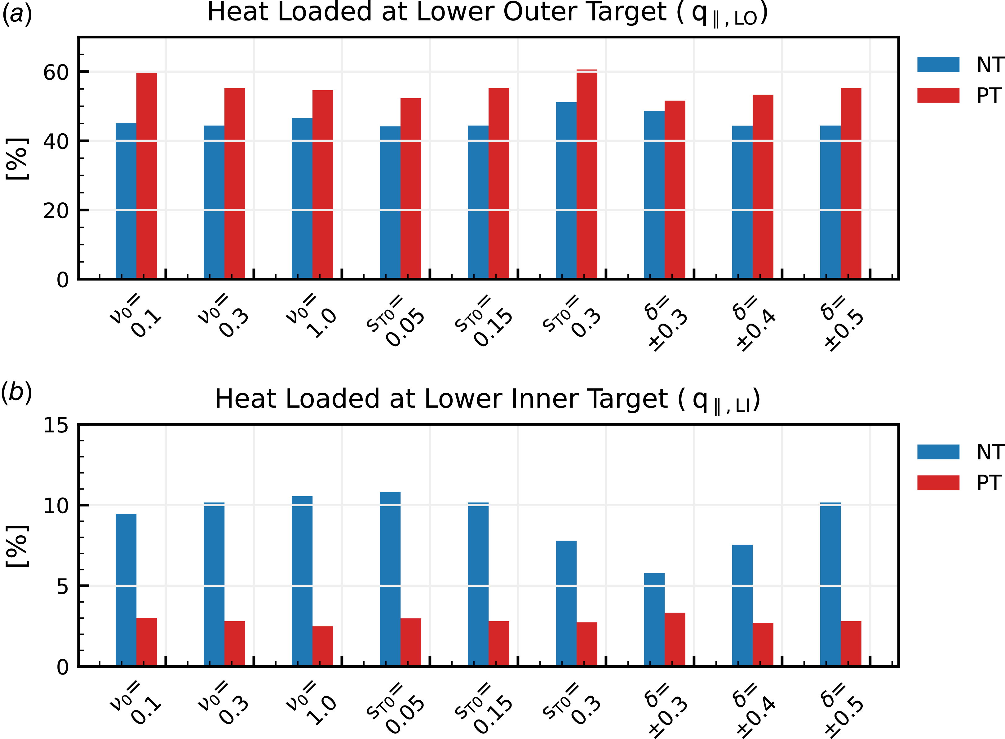


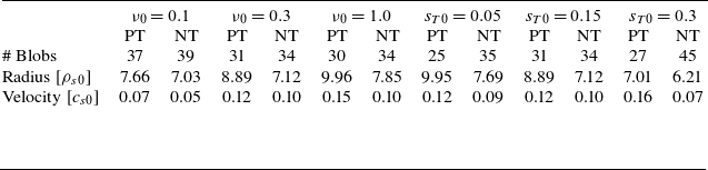


 Open access