1 - Fundamentals of Wireless Power Transfer

Summary

This chapter introduces the principles and mechanisms behind wireless power transfer (WPT), focusing on inductive power transfer systems. It begins with the historical development of WPT and then delves into the fundamental aspects of inductive power transfer, including general configurations. The chapter provides a detailed examination of theoretical models, such as the loosely coupled transformer model, T-model, and M-model, and compares their effectiveness. It further explores compensation networks, including series and parallel types, and discusses transmission performance metrics such as output power, transfer efficiency, and their interrelationships. This comprehensive overview establishes the foundational knowledge necessary for understanding advanced WPT systems.

Wireless power transfer (WPT) is a revolutionary technique that enables power to be supplied to airborne loads in a non-contact manner. It has the advantages of electrical isolation, safety, and flexibility [1]. The technology has received extensive attention from academia and industry and is widely used in electric vehicles [2, 3], unmanned aerial vehicles (UAVs) [4–6], wireless motors [7], [8], and household equipment [9, 10]. For UAVs, since flight times are typically only about 30 minutes [11] and are in dire need of extension, WPT offers an attractive solution versus physically replacing drone batteries. The origins of WPT can be traced back to the late nineteenth century, about 100 years ago.

1.1 The Origins of Wireless Power Transfer

In the late nineteenth century, Nikola Tesla first proposed WPT technology and developed a wireless lighting system that used inductive and capacitive near-field coupling. He gave public demonstrations and lectures on the technology at Columbia College, lighting Geissler tubes and incandescent bulbs from across the stage [12]. In order to realize WPT at that time, an ‘oscillating transformer’ was applied to generate high-voltage, low-current, and high-frequency alternating current, which later became known as a ‘Tesla coil’. Nikola Tesla observed that the transfer distance could be extended when the receiver’s inductor and capacitor (LC) circuit was adjusted to resonate together on the LC circuit of the transmitter [13] – that is, resonant inductive coupling.

In 1901, Tesla built a famous tower in Shoreham, New York, known as the Walden Clifford Tower, using an investment of $150,000. The purpose of this tower was to wirelessly transmit electricity and for use in experiments in transatlantic radio broadcasting. The project stalled by 1905 due to Tesla’s financial problems and a lack of new investment.

Over the next few decades, although Tesla worked on it with the help of a number of different investors, the WPT technology was not commercialized as a full-fledged product due to the limitations of the period in terms of semiconductor materials, power electronics, and manufacturing. Although this research on WPT did not continue in the early twentieth century, Tesla opened up a whole new field of research, and thus he is known as the father of wireless power transfer [14].

After nearly a century of stagnation in WPT technology, in 2007, at the US Massachusetts Institute of Technology (MIT), Professor Marin Soljacic and his research team succeeded in lighting a 60 W electric bulb from about 2 m away, with a transmission efficiency of 40%. They used two 30 cm radius primary and pickup resonator coils and adjusted the resonant frequency of the primary circuit so that both coils resonated at 10 MHz. By exploiting this magnetic field resonance (i.e. the principle of magnetic coupling resonance), they succeeded in lighting the bulb. This method not only makes up for the short transmission distance defects of inductive non-contact WPT technology, and improves the transmission distance to the metre range, it also greatly reduces the impact of energy transmission on the environment due to its low electromagnetic radiation. These researchers published their results in Science in 2007 [15]; the news attracted widespread attention in the academic community and set off a new round of WPT technology research.

1.2 Inductive Power Transfer

Wireless power transfer utilizes a transmitter to generate an electromagnetic field to transmit energy via non-contact means through space, such as air, to a receiving device, thus enhancing the versatility and reliability of electronic equipment. WPT can be mainly categorized into two types based on the different transmission distances: close-field and far-field power transfer (also known as near-field and long-field power transfer, respectively).

Close-field transmission mainly consists of capacitive power transfer (CPT) and inductive power transfer (IPT). For near-field transmission, inductive coupling between coils or capacitive coupling between capacitor plates is utilized to transmit power over short distances, which can be used in electric vehicles, UAVs, and household equipment. Far-field transmission mainly includes acoustic, optical, and microwave WPT, where power is transmitted through beams of electromagnetic radiation. It is used in space technology and military applications, such as for energy transfer between space stations and spacecraft. Although a larger transfer distance can be achieved by this means, the transmitter needs to be aimed at the receiver. Currently, IPT has the most promising development and application prospects, which we explore further below.

1.2.1 Fundamentals

Researchers around the world have extensively studied the IPT system, dividing it into transmitting and receiving components, as illustrated in Fig. 1.1. The generation of a high-frequency AC signal can be achieved using the DC power supply and an inverter, which is driven using the pulse width modulation (PWM) output. By utilizing electromagnetic induction, the transmitting current is transferred from the primary coil to the coupling pickup coil without a cable connection, which provides greater safety and flexibility [16]. Employing the principle of magnetic resonance, a suitable compensation topology is used for the primary and pickup coils so that the circuits satisfy the resonance state – that is, the magnetic coupling resonance (MCR) is realized, which ensures medium-distance WPT.

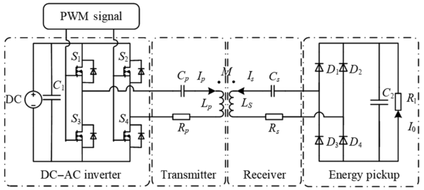
Figure 1.1 Inductive power transfer.

Figure 1.1Long description

The block diagram shows a wireless power transfer system starting from a P W M signal that drives four switches in an H - bridge D C - A C inverter. This is connected to a transmitter coil L p, in series with a capacitor C p and a resistor R p, transferring energy via mutual inductance M to a receiver coil L s in series with its own capacitor C s and resistor R s. The receiver output is connected to an energy pickup circuit with diodes D 1 to D 4, forming a full-bridge rectifier, followed by a load resistor R l through which current I D C flows. Labels also indicate A C current paths I p and I s.

Using the principle of magnetic resonance from the physical world, in 2007 Professor Marin Soljacic of MIT designed some experiments to verify the MCR system – that is, to ensure the transmitting resonator resonates at the same frequency as the receiving resonator. He discovered that electrical energy can be transmitted between these resonators. This famous WPT experiment effectively verified the MCR mechanism at a distance of 2 m and transmission power of 60 W [15]. In order to further analyse and enhance the transfer efficiency and range of this WPT system, other scholars have expanded upon the theoretical analysis by modelling and analysing the system using equivalent circuits and Neumann’s formula [17]. For a typical application of wireless energy transmission (e.g. a hovering UAV wireless charging system), a novel estimation scheme of mutual inductance has been designed based on high-order circuit topology, and a constant-current controller has been designed to ensure constant output current control without receiver-side current feedback [18]. High-order compensation topologies are employed in this context to achieve load-independent constant-current output characteristics.

In some of the literature, magnetically induced WPT systems have been categorized into two types: the IPT system and the MCR system. The IPT system is described as a type of WPT between transmitter and receiver coils in close proximity by means of magnetic coupling based on the transformer principle. The MCR WPT system ensures that the transmitting and receiving mechanisms are in a common resonance state, and utilizes the energy coupling principle to realize WPT over medium distances. In IPT systems the actual compensating capacitance is used to resonate with the coil, while MCR systems use the designed parasitic capacitor to balance and compensate for the impedance. The fundamentals and operating principles of the two categories are essentially identical, but the quality factor (Q) of the coil is usually higher in the MCR system to ensure greater coupling [19]. Therefore, instead of distinguishing between these two systems in this book, the more representative IPT system is used to illustrate the magnetic induction-based WPT system.

Figure 1.2 shows the principle behind the IPT system, where the AC voltage is supplied to the load side in a non-contact manner through the transmitting and receiving coils. The specific power transfer process is described as follows:

1. 1. A high-frequency inverter is used to convert the DC voltage generated from a DC power source into a high-frequency AC voltage (from tens of kilohertz [20, 21] to a few megahertz [22]), which is the input to the WPT system.

2. 2. The AC voltage is input to the coil inductor and compensation capacitor of the primary side at resonance, while the alternating current flowing through the transmitting coil produces an alternating induced magnetic field.

3. 3. The alternating induced magnetic field of a given frequency produced by the transmitting coil induces an alternating inductive voltage of the identical frequency in the receiving coil through weak coupling.

4. 4. After capacitive compensation, rectification, and filtering on the receiving side, the induced AC voltage is transformed into a DC voltage and transmitted to the power-using equipment.

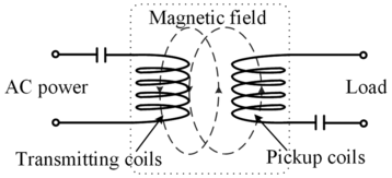
Figure 1.2 The principle of IPT.

Figure 1.2Long description

This simplified conceptual diagram shows two sets of coils, transmitting coils on the left connected to an A C power source, and pickup coils on the right connected to a load. A magnetic field is shown flowing from the transmitting to the pickup coils, indicating inductive coupling. This represents wireless energy transfer via magnetic induction.

From the above elaboration, it can be seen that the principle of the IPT system is familiar to traditional transformer theory. So what are the differences between them? In the following, we discuss four important characteristics of IPT systems that differ from transformers.

Lesser Coupling Coefficients

Due to the existence of a transfer distance between the two coils in this IPT system, the resulting leakage inductance is generally hundreds of times greater than that of a transformer. The larger air gap also greatly reduces the magnetic flux, resulting in a lower mutual inductance coefficient M and a weaker coupling coefficient in this IPT system [23]. Therefore, to obtain higher Q coils and enhance the system coupling coefficient, the optimized design of the coupling coils and the reasonable selection of compensation topology are key difficulties in the IPT system.

Hollow-Core Inductor

In IPT systems, power transfer between the primary and pickup devices can be realized by magnetic coupling between inductors, most of which are hollow inductors in order to avoid core-induced energy loss. The difference is that transformer windings usually use cores to form the magnetic circuit of the system to minimize energy loss due to magnetic leakage. Therefore, whether or not a core is used as the magnetic circuit can be a critical factor in distinguishing a conventional transformer from an IPT system.

Phase Difference

For an ideal transformer, if we ignore losses such as leakage inductance, the transmitter and receiver currents may be the equal or reverse of each other; for an IPT system the phase difference of the transmitter- and receiver-side currents can usually be about 90 degrees because of the impedance adjustment of the compensation capacitors.

System Disturbances and Parasitic Parameters

As the transfer distance between coils, angular/lateral misalignment, and load values fluctuate, the intrinsic and reflective values of an IPT system vary dramatically, resulting in dynamic changes in output power and efficiency. Furthermore, in common high-frequency IPT systems it is important to note that parasitic resistors and parasitic capacitors have a significant impact on the system transfer capability. Therefore, how to maintain great transfer efficiency and robust output behaviour in the presence of complicated parametric disturbances and parasitic parameters is a key challenge for IPT systems.

This section has provided a comprehensive overview of the IPT principle, including the system components and the differences in the principle relative to conventional transformers. The general configuration of IPT systems is described next.

1.2.2 General Configuration

As shown in Fig. 1.3, a common IPT system configuration uses only one transmitter and one receiver, with typical components including: primary-side energy supply, transmitter-side compensated topology, magnetic coupler, receiver-side compensated topology, and receiver device.

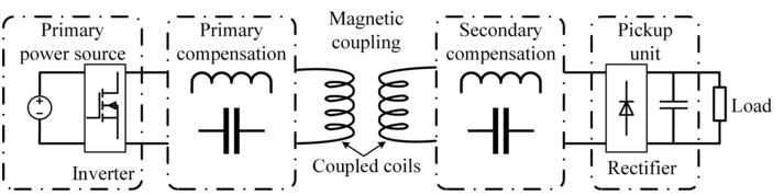
Figure 1.3 Configuration of an IPT system.

Figure 1.3Long description

This schematic diagram breaks down a wireless power system into five labeled blocks, Primary power source and inverter, shows a voltage source connected to an inverter.Primary compensation, a capacitor compensating the transmitting coil. Magnetic coupling, coupled coils, transmitting and receiving coils aligned for inductive power transfer. Secondary compensation, another capacitor used for tuning the receiving side. Pickup unit and rectifier, includes a rectifier circuit that converts A C to D C, which then powers the load. Arrows indicate the flow of power from left, input to right, output.

Primary-Side Power Source

An inverter is the key component for converting DC voltage into the high-frequency AC voltage used in IPT systems. Half- or full-bridge class D inverters have been widely used in low- and medium-power IPT systems for their simple parameter setup and ease of control. However, since the surge voltage flowing through the switching tubes is generally double that of the input voltage, the switching tubes face the risk of breakdown at high voltages. To address this problem, the parallel and cascaded inverters can be adopted to achieve increased output power with improved flexibility [24]. It is worth noting that the combination of signal generator and power amplifier can also generate an AC input voltage to power the IPT system; this has lower total harmonic distortion (THD) but poorer efficiency performance.

Primary/Secondary-Side Compensation Topology

A specially designed compensation topology can eliminate the large leakage inductive reactance in the IPT loosely coupled system by means of several LC resonant tanks, minimizing the primary-side voltage-ampere (VA) rating and maximizing the receiver-side efficiency [25, 26]. In the primary and secondary resonant circuits, the coil inductances resonate with the capacitances of the capacitors. Meanwhile, the LC resonant circuit filters out harmonics in other frequency bands and modulates the transmitter current to a sinusoidal waveform.

Common compensation topologies are series or parallel compensation, and some high-order topologies such as the LCC topology can be used to achieve a constant load-independent output under parametric disturbances, or to implement soft-switching techniques to maximize the transmission efficiency of the IPT system. In high-frequency IPT systems, MOSFETs (metal-oxide-semiconductor field-effect transistors) are often used for inverter switching components, and the implementation of soft-switching techniques can effectively reduce switching power loss and thus greatly improve the overall transfer efficiency.

In conclusion, a proper selection of the compensation network and the optimal parameter design of the LC compensation topology can greatly benefit the transfer properties of the IPT system.

Magnetic Coupling

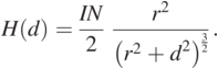
Figure 1.4 illustrates a simplified solenoidal magnetic coupling system in an IPT system. Here, r is the coil radius and d is the transmission distance. According to the Biot–Savart theorem, the strength of the electromagnetic force at a point is:

$H\left(d\right)=\frac{\mathit{\text{IN}}}{2}\frac{r^2}{{\left(r^2+d^2\right)}^{\frac{3}{2}}}.$(1.1)

Based Eq. (1.1), the magnetic field strength is enhanced along with the increase of the primary current I or the increase of the number of turns N of the coil. Theoretically, the higher the magnetic field strength of the WPT system, the higher the output power, but the calculation of r, d, and the magnetic field strength is complicated. In the plot shown in Fig. 1.5, the horizontal coordinate is the ratio of d to r and the vertical coordinate is the normalized magnetic field strength. It can be seen that the normalized magnetic field strength increases slowly and then decreases sharply as the horizontal coordinate d/r increases. Based on Eq. (1.1), it can be found that at the peak of the magnetic field, the ratio of transmission distance d to radius r is 1/sqrt(2). Therefore, transmission performance is better when the transfer distance is the radius of the transmitting coil.

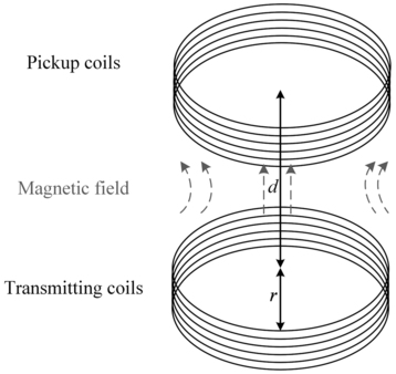
Figure 1.4 A simplified magnetic coupling system.

Figure 1.4Long description

A 3D schematic illustrates a pair of circular coils, the transmitting coils at the bottom and the pickup coils at the top. The coils are aligned vertically with a separation distance labeled as d. Curved arrows between the coils depict the magnetic field lines rising from the transmitting coil and entering the pickup coil, illustrating the principle of inductive energy transfer. Both coils are shown as multi-turn windings.

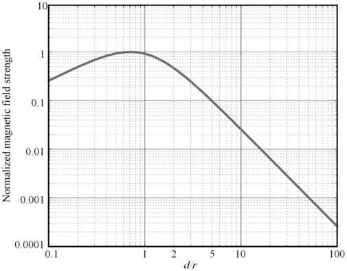
Figure 1.5 The system magnetic field strength.

Figure 1.5Long description

The graph presents a log–log plot of normalized magnetic field strength, y-axis against relative distance d r, x-axis. The curve rises initially, reaching a peak near d r = 1, then declines steeply. The x-axis spans from 0.1 to 100, and the y-axis from 0.0001 to 10. The trend illustrates that magnetic field strength is highest at a certain proximity and drops rapidly as the coils are placed further apart, indicating optimal spacing for inductive coupling.

Receiver Unit

Generally, a rectifier bridge is used to transform the AC current to DC current on the receiving side, followed by a filter capacitor to reduce the voltage ripple. In addition, the DC–DC converter may be required to stabilize the load voltage or current, depending on the required load voltage or current of the power-using equipment. The converter can also be adjusted with a switching duty cycle to be applied as an impedance transformer.

1.3 Theoretical Modelling

Figure 1.3 shows the structure of a single-transmitter and single-receiver IPT system, where the loosely coupled transmitter-side and receiver-side coils are not mechanically or electrically connected, but rather the power is transmitted through an induced magnetic field. Therefore, magnetic coupling is the key component of the IPT system required to realize power transmission. Here, we begin by describing the basic fundamentals of loosely coupled transformers.

1.3.1 The Model for Loosely Coupled Transformers

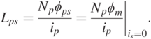
For practical loosely coupled transformer systems, a large leakage inductance and leakage flux are generated because of the long transfer distance of the coupling coils. Figure 1.6 shows a coupled transformer with leakage flux, where the flux distribution of the coupling coils is depicted.

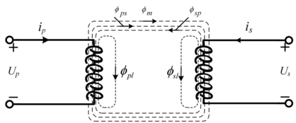
Figure 1.6 A schematic diagram of loosely coupled transformers.

Figure 1.6Long description

This schematic shows two coils, the left coil is labeled with voltage U p, current i p, and the right coil with voltage U s, current i s. The magnetic flux paths are shown with dashed lines, phi p l, phi p s, and phi m. The magnetic coupling between coils is denoted via the shared flux phi m, while leakage fluxes phi p l and phi s l represent uncoupled parts.

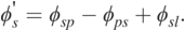
In Figure 1.6 ${\varphi }_{\mathit{ps}}$ represents the flux produced by the primary coil passing through the pickup coil, and ${\varphi }_{\mathit{pl}}$ represents the flux passing elsewhere; similarly, ${\varphi }_{\mathit{sp}}$ represents the flux generated by the pickup coil passing through the primary coil and ${\varphi }_{\mathit{sl}}$ represents the flux passing elsewhere. In addition, U_p, I_p, U_s, and I_s represent the primary current voltage and the secondary current voltage, respectively; ${\varphi }_m$ represents the shared flux:

${\varphi }_m={\varphi }_{\mathit{ps}}-{\varphi }_{\mathit{sp}}.$(1.2)

In this case, the equivalent magnetic flux produced in the primary coil is:

${\varphi }_p^{’}={\varphi }_{\mathit{ps}}-{\varphi }_{\mathit{sp}}+{\varphi }_{\mathit{pl}}.$(1.3)

In a similar way, the equivalent magnetic flux produced in the pickup coil is:

${\varphi }_s^{’}={\varphi }_{\mathit{sp}}-{\varphi }_{\mathit{ps}}+{\varphi }_{\mathit{sl}}.$(1.4)

Therefore, the primary-side input voltage and charging voltage are:

$\begin{array}{l}{U}_p=N_p\frac{d{\varphi }_p^{’}}{\mathit{dt}}=N_p\frac{d\left({\varphi }_{\mathit{pl}}+{\varphi }_{\mathit{ps}}-{\varphi }_{\mathit{sp}}\right)}{\mathit{dt}}=L_{\mathit{pl}}\overrightarrow{i_p}+\left(L_{\mathit{ps}}\overrightarrow{i_p}-\frac{L_{\mathit{sp}}\overrightarrow{i_s}}{n}\right),\\ U_s=N_s\frac{d{\varphi }_s^{’}}{\mathit{dt}}=N_s\frac{d\left({\varphi }_{\mathit{sl}}+{\varphi }_{\mathit{sp}}-{\varphi }_{\mathit{ps}}\right)}{\mathit{dt}}=L_{\mathit{sl}}\overrightarrow{i_s}+\left(L_{\mathit{sp}}\overrightarrow{i_s}-{\mathit{nL}}_{\mathit{ps}}\overrightarrow{i_p}\right).\end{array}$(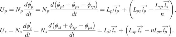1.5)

Here, N_p and N_s are the turns of the primary and secondary windings. In addition, the relative inductance and turns ratio n can be indicated as:

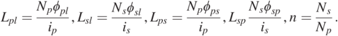
$L_{\mathit{pl}}=\frac{N_p{\varphi }_{\mathit{pl}}}{i_p},L_{\mathit{sl}}=\frac{N_s{\varphi }_{\mathit{sl}}}{i_s},L_{\mathit{ps}}=\frac{N_p{\varphi }_{\mathit{ps}}}{i_p},L_{\mathit{sp}}\frac{N_s{\varphi }_{\mathit{sp}}}{i_s},n=\frac{N_s}{N_p}.$(1.6)

In this case, the equation of the transformer magnetic circuit is expressed in the following way:

$N_p{i}_p=N_s{i}_s=\mathrm{\Re }{\varphi }_m,$(1.7)

where $\mathrm{\Re }$ is the magnetoresistance of the coil. Following this, L_ps can be recalculated as:

$L_{\mathit{ps}}=\frac{N_p{\varphi }_{\mathit{ps}}}{i_p}={\left.\frac{N_p{\varphi }_m}{i_p}\right|}_{i_s=0}.$(1.8)

By substituting Eq. (1.7) into Eq. (1.8), L_ps is expressed as:

$L_{\mathit{ps}}=\frac{N_p^2}{\mathrm{\Re }}.$(1.9)

Similarly, L_sp can be derived as:

$L_{\mathit{sp}}=\frac{N_s^2}{\mathrm{\Re }}.$(1.10)

According to Eqs. (1.9) and (1.10), the relationship of L_sp and L_ps can be expressed as:

$L_{\mathit{sp}}=n^2{L}_{\mathit{ps}}.$(1.11)

By substituting Eq. (1.11) into Eq. (1.5), it can be concluded that:

$\begin{array}{l}{U}_p=L_{\mathit{pl}}\overrightarrow{i_p}+\left(L_{\mathit{ps}}\overrightarrow{i_p}-\frac{L_{\mathit{sp}}\overrightarrow{i_s}}{n}\right)=L_{\mathit{pl}}\overrightarrow{i_p}+L_{\mathit{ps}}\left(\overrightarrow{i_p}-n\overrightarrow{i_s}\right),\\ U_s=L_{\mathit{sl}}\overrightarrow{i_s}+\left(L_{\mathit{sp}}\overrightarrow{i_s}-{\mathit{nL}}_{\mathit{ps}}\overrightarrow{i_p}\right)=L_{\mathit{sl}}\overrightarrow{i_s}-{\mathit{nL}}_{\mathit{ps}}\left(\overrightarrow{i_p}-n\overrightarrow{i_s}\right),\\ U_m=L_{\mathit{ps}}\left(\overrightarrow{i_p}-n\overrightarrow{i_s}\right).\end{array}$(1.12)

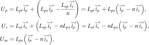
Therefore, the circuit in Fig. 1.7 is constructed according to Eq. (1.12), which is composed of an ideal transformer.

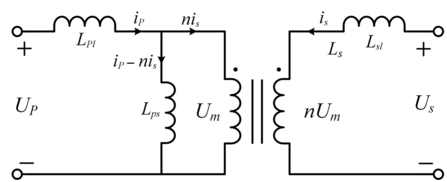
Figure 1.7 A loosely coupled transformer model.

Figure 1.7Long description

The circuit shows a transformer equivalent model separated into two parts. The left side represents the primary with source voltage U p, primary current i p, and leakage inductance L p l. A magnetizing branch with inductance L p m connects to magnetizing voltage U m. The secondary side has induced voltage U m, current i s, and inductors L s and L s l representing secondary leakage and winding inductance. Turns ratio n and current ratio eta i are labeled, showing how energy is transferred from the primary to the secondary.

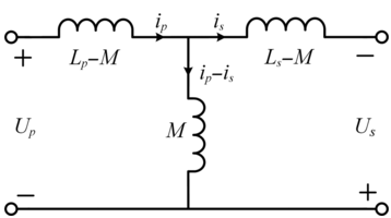
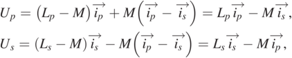
1.3.2 T-model

The T-model is illustrated in Fig. 1.8. It is called the T-model because the three inductors in its topology are similar to the letter T. The following equation is satisfied: M = nL_ps, L_p = L_pl + L_ps, L_s = L_sl + L_sp. By replacing Eq. (1.11) into Eq. (1.12), we obtain:

$\begin{array}{l}{U}_p=L_{\mathit{pl}}\overrightarrow{i_p}+L_{\mathit{ps}}\left(\overrightarrow{i_p}-n\overrightarrow{i_s}\right)=\left(L_{\mathit{pl}}+L_{\mathit{ps}}-{\mathit{nL}}_{\mathit{ps}}\right)\overrightarrow{i_p}+{\mathit{nL}}_{\mathit{ps}}\left(\overrightarrow{i_p}-\overrightarrow{i_s}\right)=\left(L_p-M\right)\overrightarrow{i_p}+M\left(\overrightarrow{i_p}-\overrightarrow{i_s}\right),\\ U_s=L_{\mathit{sl}}\overrightarrow{i_s}+\left(L_{\mathit{sp}}\overrightarrow{i_s}-{\mathit{nL}}_{\mathit{ps}}\overrightarrow{i_p}\right)=\left(L_{\mathit{sl}}+L_{\mathit{sp}}-{\mathit{nL}}_{\mathit{ps}}\right)\overrightarrow{i_s}-{\mathit{nL}}_{\mathit{ps}}\left(\overrightarrow{i_p}-\overrightarrow{i_s}\right)=\left(L_s-M\right)\overrightarrow{i_s}-M\left(\overrightarrow{i_p}-\overrightarrow{i_s}\right).\end{array}$(1.13)

Figure 1.8 The T-model for one-to-one transmission.

Figure 1.8Long description

This schematic illustrates a mutual inductance model for a transformer. The primary side includes voltage U p, current i p, and inductance L p - M. The secondary has voltage U s, current i s, and inductance L s - M. The mutual inductance M links both coils, with the central branch carrying current i p i s.

1.3.3 M-model

The M-model (Fig. 1.9) is a common theoretical model applied to IPT systems. According to Eq. (1.13), the theoretical formulation of the M-model is derived as:

$\begin{array}{l}{U}_p=\left(L_p-M\right)\overrightarrow{i_p}+M\left(\overrightarrow{i_p}-\overrightarrow{i_s}\right)=L_p\overrightarrow{i_p}-M\overrightarrow{i_s},\\ U_s=\left(L_s-M\right)\overrightarrow{i_s}-M\left(\overrightarrow{i_p}-\overrightarrow{i_s}\right)=L_s\overrightarrow{i_s}-M\overrightarrow{i_p},\end{array}$(1.14)

where M represents the mutual inductance of coils:

$M={\mathit{nL}}_{\mathit{ps}}.$(1.15)

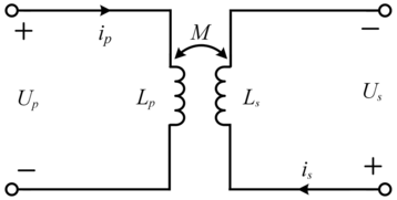
Figure 1.9 M-model for one-to-one transmission.

Figure 1.9Long description

The circuit shows a transformer with mutual inductance M between two inductors, primary coil with inductance L p and voltage U p, and secondary coil with inductance L s and voltage U s. Currents i p and i s flow in opposite directions in the two windings.

1.4 Compensation Network

Because of the high-leakage inductive reactance of IPT systems, without matching the compensation capacitors both the transmitter and receiver sides will consume a lot of power, thus reducing the system’s power factor. Therefore, reactive power compensation is extremely important to improve the system transfer efficiency.

In general, capacitive compensation is a common method of removing inductive reactance in IPT systems. It is based on the principle of utilizing capacitors in a well-designed compensation network to resonate with the coil self-inductance, hence eliminating the system reactive power. Typically, the compensation circuits can be categorized into two forms, series type and parallel type, based on the connection between the capacitors and inductors.

1.4.1 Series Type

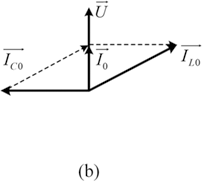
For the RLC circuit illustrated in Fig. 1.10(a), the equivalent impedance Z_s is:

$Z_s=R+\mathit{j\omega L}+\frac{1}{\mathit{j\omega C}}=R+j\left(\mathit{\omega L}-\frac{1}{\mathit{\omega C}}\right)=R+\mathit{jX}=\left|Z\right|\angle \phi ,$(1.16)

where X is the imaginary part of Z_s. Setting X = 0, ${\omega }_0$ is determined as:

${\omega }_0=\frac{1}{\sqrt{\mathit{LC}}}.$(1.17)

f₀ can be expressed as:

$f_0=\frac{1}{2\pi \sqrt{\mathit{LC}}}.$(1.18)

Figure 1.10

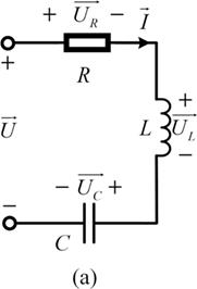
(a) Series-type circuit;

Figure 1.10(a)Long description

A series R L C circuit includes a voltage source U, a resistor R, an inductor L, and a capacitor C, connected in series. The voltage drops are labeled as U R, U L and U C. Arrows indicate current direction I. Polarity is marked for each component, the capacitor is charged with negative on the top and positive on the bottom. Voltage sum relations are suggested by U R plus U L minus U C = U.

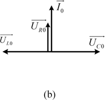
(b) series resonance vector.

Figure 1.10(b)Long description

This phasor diagram shows three orthogonal vectors, U R 0 pointing right, U C 0 pointing downward, and U L 0 pointing upward. The phasors visually represent the voltage drops across components in the R L C circuit from the previous diagram. The resultant phasor U is the sum of these components and indicates the total applied voltage.

According to Eqs. (1.17) and (1.18), the series resonance is characterized as follows. The voltage across the inductor (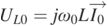$U_{L0}=j{\omega }_{0}L\overrightarrow{I_0}$) and the voltage across the capacitor (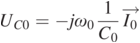$U_{C0}=-j{\omega }_0\frac{1}{C_0}\overrightarrow{I_0}$) have the same amplitude and opposite phase. Thus, the LC resonant tank is equivalent to a short circuit and all voltages are supplied to the resistor, as shown in Fig. 1.10(b).

The quality factor (Q) of a resonant circuit can be defined by the ratio of the resonant inductor voltage or resonant capacitor voltage to the supply voltage:

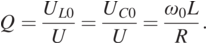$Q=\frac{U_{L0}}{U}=\frac{U_{C0}}{U}=\frac{{\omega }_{0}L}{R}.$(1.19)

1.4.2 Parallel Type

The IPT system with parallel capacitor compensation is illustrated in Fig. 1.11(a). Z_p is expressed as:

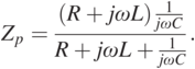$Z_p=\frac{\left(R+\mathit{j\omega L}\right)\frac{1}{\mathit{j\omega C}}}{R+\mathit{j\omega L}+\frac{1}{\mathit{j\omega C}}}.$(1.20)

Assuming Im{Z_p} = 0, ${\omega }_0$ is obtained by:

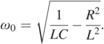${\omega }_0=\sqrt{\frac{1}{\mathit{LC}}-\frac{R^2}{L^2}}.$(1.21)

Figure 1.11

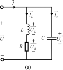
(a) Parallel-type circuit;

Figure 1.11(a)Long description

The diagram shows a parallel R L C circuit with an A C voltage source U applied across all components. Branches include, inductor L, resistor R, and capacitor C. Current splits into I L, I R and I C respectively. Voltage drops U L, U R and U C are marked. The direction of total current I entering the junction is shown at the top. Voltages across all branches are equal due to parallel configuration.

(b) parallel resonance vector.

Figure 1.11(b)Long description

This phasor diagram represents the vector addition of current components in a parallel R L C circuit. I C points upward, I L points downward, and the total current I lies at an angle, formed by summing these components. The resultant vector I shows the combined effect of inductive and capacitive currents relative to the applied voltage.

Equation (1.21) needs to satisfy $R<\sqrt{\frac{L}{C}}$. f₀ can be expressed as:

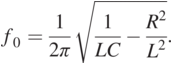$f_0=\frac{1}{2\pi }\sqrt{\frac{1}{\mathit{LC}}-\frac{R^2}{L^2}}.$(1.22)

Figure 1.11(b) illustrates the parallel-type vector map. Some higher-order topologies have been applied to achieve the desired output characteristics, such as constant current.

Because of the advantages of the simplicity of the structure and independence of the parameter design, this chapter focuses on the primary-side series–secondary-side series (SS) compensation network for the transmission performance.

1.5 Transmission Performance

This section analyses the transmission performance of the most common SS compensated network for single-transmitter–single-receiver IPT systems, focusing on the output power, output efficiency, and their influencing factors.

1.5.1 Output Power

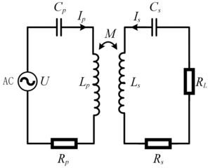
The IPT system in SS topology is shown in Fig 1.12. Its circuit equations are:

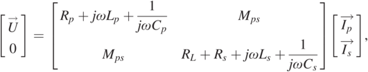$\left[\begin{array}{c}\overrightarrow{U}\\ 0\end{array}\right]=\left[\begin{array}{cc}{R}_p+\mathit{j\omega }{L}_p+\frac{1}{\mathit{j\omega }{C}_p}& M_{\mathit{ps}}\\ M_{\mathit{ps}}& R_L+R_s+\mathit{j\omega }{L}_s+\frac{1}{\mathit{j\omega }{C}_s}\end{array}\right]\left[\begin{array}{c}\overrightarrow{I_p}\\ \overrightarrow{I_s}\end{array}\right],$(1.23)

where L, C, and R, subscripted as p or s, are the transmitting and receiving inductance, compensation capacitance, and coil internal resistance, respectively. The system load and mutual inductance between the coupling coils are R_L and M_ps, respectively.

Figure 1.12 A simplified IPT system with SS compensation network.

Figure 1.12Long description

This schematic shows a full wireless power transfer model with coupled inductors. An A C voltage source feeds into the primary loop, which includes a capacitor C p, inductor L p, and resistor R p. The primary coil couples magnetically, via mutual inductance M with the secondary loop, which includes inductor L s, capacitor C s, and resistor R s. Arrows label the current in each loop as I p and I s, and the mutual coupling allows power transfer from primary to secondary.

When the system impedance is matched, Eq. (1.24) can be derived:

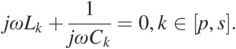$\mathit{j\omega }{L}_k+\frac{1}{\mathit{j\omega }{C}_k}=0,k\in \left[p,s\right].$(1.24)

Replacing Eq. (1.24) into Eq. (1.23), the current I_p and $\overrightarrow{I_s}$ are derived as:

$\begin{array}{l}{I}_p=\frac{U}{R_p+\frac{{\omega }^2{M}_{\mathit{ps}}^2}{R_s+R_L}}=\frac{U}{Z_{\mathit{\text{in}}}},\\ \overrightarrow{I_s}=\frac{-\mathit{j\omega }{M}_{\mathit{ps}}U}{R_p\left(R_s+R_L\right)+{\omega }^2{M}_{\mathit{ps}}^2}.\end{array}$(1.25)

The reflected impedance Z_r from the receiver to the transmitter can be calculated as:

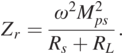$Z_r=\frac{{\omega }^2{M}_{\mathit{ps}}^2}{R_s+R_L}.$(1.26)

According to Eq. (1.25), the input power P_in and the output power P_L are derived as:

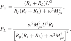$\begin{array}{l}{P}_{\mathit{\text{in}}}=\frac{\left(R_s+R_L\right)U^2}{R_p\left(R_s+R_L\right)+{\omega }^2{M}_{\mathit{ps}}^2},\\ P_L=\frac{{\omega }^2{M}_{\mathit{ps}}^2{U}^2{R}_L}{{\left[R_p\left(R_s+R_L\right)+{\omega }^2{M}_{\mathit{ps}}^2\right]}^2}.\end{array}$(1.27)

Here, the optimal load R_Lpmax of the largest output power is obtained as:

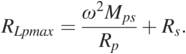$R_{\mathit{\text{Lpmax}}}=\frac{{\omega }^2{M}_{\mathit{ps}}}{R_p}+R_s.$(1.28)

Then, by substituting Eq. (1.28) into Eq. (1.27), the largest output power P_Lmax is obtained:

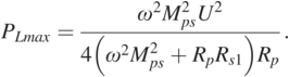$P_{\mathit{\text{Lmax}}}=\frac{{\omega }^2{M}_{\mathit{ps}}^2{U}^2}{4\left({\omega }^2{M}_{\mathit{ps}}^2+R_p{R}_{s1}\right)R_p}.$(1.29)

1.5.2 Transfer Efficiency

It is worth noting that the transfer efficiency of an IPT system is one of its key metrics. According to Eq. (1.27), the transfer efficiency η is obtained as:

$\eta =\frac{P_L}{P_{\mathit{\text{in}}}}=\frac{{\omega }^2{M}_{\mathit{ps}}^2{R}_L}{\left[R_p\left(R_s+R_L\right)+{\omega }^2{M}_{\mathit{ps}}^2\right]\left(R_s+R_L\right)}.$(1.30)

The optimal load R_Lηmax of the greatest efficiency is obtained as:

$R_{\mathit{\text{Lηmax}}}=R_{s1}\sqrt{1+\frac{{\omega }^2{M}_{\mathit{ps}}^2}{R_p{R}_s}}.$(1.31)

Then, based on Eqs. (1.31) and (1.30), the greatest efficiency is obtained as:

${\eta }_{\mathit{max}}=1-\frac{2}{\sqrt{1+\frac{{\omega }^2{M}_{\mathit{ps}}^2}{R_p{R}_s}}+1}.$(1.32)

Therefore, according to Eq. (1.32), it can be found that to obtain a larger transfer efficiency, it is theoretically possible to reduce the coil internal resistance and increase the coupling effect of the coils.

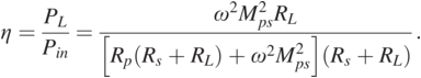
1.5.3 The Relationship between Output Power and System Efficiency

To further illustrate the coupling between output power and system efficiency, Fig. 1.13 shows the efficiency and normalized load power against Z_r/R_p. It can be seen that the normalized load power initially rises rapidly then falls slightly with increasing values of Z_r/R_p. It is worth noting that the maximum output power is reached when Z_r/R_p = 1 is satisfied. In addition, the transfer efficiency rises nonlinearly as Z_r/R_p increases, eventually approaching 1.

Figure 1.13 Efficiency and normalized load power versus Z_r/R_p.

Figure 1.13Long description

This graph plots two curves against the x-axis labeled Z r by R p, load-to-resistance ratio, ranging from 0 to 12. The y-axis shows values from 0 to 1. The solid line represents the normalized delivered power P d by P L max, which peaks early and declines. The dashed line represents efficiency, which increases rapidly and then levels off. The plot illustrates that while power transfer peaks at a certain load ratio, efficiency continues to rise with increased load impedance.