


Nomenclature
- $t$
$t$
-
time, s
-
$\theta$
-
aircraft pitch, rad
-
$\text{ }\!\!\Lambda\!\!\text{ }$
-
wing symmetric sweep, positive forward, rad
-
$\text{ }\!\!\Gamma\!\!\text{ }$
-
wing symmetric dihedral, positive upward, rad
-
$\text{ }\!\!\Phi\!\!\text{ }$
-
wing symmetric incidence angle, positive upward, rad
-
$\alpha$
-
local effective angle-of-attack, rad
-
${{\beta }_{e}}$
-
elevator deflection, rad
-
$U$
-
airspeed, m/s
-
$\mathbf{U}$
-
airspeed vector, m/s
-
${{b}_{c}}$
-
semichord, m
-
${{c}_{c}}$
-
chord, m
-
$\rho$
-
air density, 1.2 kg/m3
-
${{C}_{i}}$
-
aerodynamic coefficient
- Re
-
Reynolds number
-
${{\tau }_{i}}$
-
Goman-Khrabrov delay parameter
-
$p$
-
Goman-Khrabrov mixing parameter
-
${{p}_{0}}$
-
Goman-Khrabrov quasistatic mixing function
-
${{a}_{i}}$
, …,
${{e}_{i}}$
-
aerodynamic coefficient fitting parameters
-
$S\!\left( \cdot \right)$
-
logistic function
-
$\phi$
-
location of logistic curve halfway point
-
$m$
-
logistic curve gradient parameter
-
$M$
-
width of one-sided Gaussian
-
$w$
-
height of one-sided Gaussian
-
$k$
-
normalised parameter for elevator deflection
-
$\kappa$
-
local reduced frequency
-
$r$
-
local reduced pitch rate
-
$\text{ }\!\!\Omega\!\!\text{ }$
-
local frequency of aerofoil motion, rad/s
-
${{F}_{\text{prop}}}$
-
thrust force, N
- T/W
-
thrust-to-weight ratio of UAV
-
$\mathbf{z}$
-
first-order system state
-
$\boldsymbol{\upsilon }$
-
control input vector
-
$\mathbf{p}$
-
vector of mixing parameters
-
$\boldsymbol{\alpha }$
-
vector of angles of attack
-
${{\text{B}}_{i}}\!\left( \cdot \right)$
,
${{\text{T}}_{i}}\!\left( \cdot \right)$
-
first-order system matrix functionals
-
$\mathbf{f}\!\left( \cdot \right)$
-
first-order system vector function
-
${\boldsymbol{\mathcal{Q}}_{\text{A}}}\!\left( \cdot \right)$
-
aerodynamic model function
-
$\mathbf{L}$
,
$\mathbf{D}$
,
$\mathbf{M}$
-
lift, drag, moment force vectors
-
$\overset{}{\hat{\mathbf{L}}}\,$
,
$\overset{}{\widehat{\mathbf{D}}}\,$
,
$\overset{}{\widehat{\mathbf{M}}}\,$
-
lift, drag, moment force unit vectors
-
$\text{I}$
-
identity matrix
-
${{\!\left[ \cdot \right]}_{\text{IV}}}$
-
Iverson bracket


Subscripts:
-
$l$
-
leading edge of aerofoil
-
$t$
-
trailing edge of aerofoil
-
$L$
-
lift
-
$D$
-
drag
-
$M$
-
pitching moment
-
$\alpha$
-
coefficient with respect to angle-of-attack
-
$\text{sep}$
-
separated flow
-
$\text{att}$
-
attached flow
-
$\text{sym}$
-
symmetric component of model
-
$\text{ref}$
-
reference value


1.0 Introduction
Birds, bats and other flying animals show manoeuvrability far beyond the performance of current unmanned aerial vehicles (UAVs) of comparable scale. Manoeuvres such as stall turns [Reference Altenbach1–Reference Tian, Iriarte-Diaz, Middleton, Galvao, Israeli, Roemer, Sullivan, Song, Swartz and Breuer3], whiffling [Reference Pete, Kress, Dimitrov and Lentink4, Reference Marchant and Higgins5], zero-airspeed rolling [Reference Warrick and Dial6] and ballistic braking [Reference Ando and Shiraishi7–Reference Jackson9] are enabled by complex wing morphing, and defy the performance limits of conventional UAVs. In addition, displays of aggression (agonistic behaviour) and predator-prey interaction by these animals involve close-quarters body reorientations [Reference Simmons and Mendelsohn10], extreme evasive manoeuvres [Reference Hedenstrom and Rosén11], and swarm coordination [Reference Brighton, Zusi, McGowan, Kinniry, Kloepper and Taylor12]. Many flying animals could indeed be characterised as supermanoeuvrable, as per by Herbst [Reference Herbst13] and Gal-Or [Reference Gal-Or14]: showing controlled post-stall manoeuvrability, and the ability to rapidly reorient themselves independent of their flight trajectory. However, existing supermanoeuvrable aircraft and UAVs have derived their capability not from bioinspiration, but from advances in thrust vectoring technology [Reference Gal-Or14, Reference Joyce15] and the study of unstable airframes [Reference Erickson16, Reference Ericsson17]. Biomimetic supermanoeuvrability has remained an understudied topic until recently [Reference Pons and Cirak18–Reference Fei, Tu, Zhang and Deng20], but with increasing interest in autonomous dogfighting UAVs [Reference Han, Cheng and Lv21, Reference Wang, Zheng, Tai, Liu and Yue22], enhancing UAV manoeuvrability is increasingly relevant.
Biomechanical studies have revealed several distinct mechanisms by which animals achieve extreme flight manoeuvrability. At smaller spatial scales, including in insects and hummingbirds, manoeuvrability is typically achieved by thrust vectoring: altering the kinematics of a high-frequency wingbeat, which also provides the majority of the lift force required to maintain flight [Reference Taylor23, Reference Walker and Taylor24]. As such, this mechanism of manoeuvrability requires flapping-wing propulsion, and cannot be isolated from it. However, at larger spatial scales, it is possible to partially distinguish between flapping-wing propulsion and morphing-wing supermanoeuvrability, as separate but related phenomena. For instance, flying squirrels, which are without any form of propulsion, show capability for supermanoeuvres such as stall turning and ballistic braking [Reference Jackson9, Reference Harris and Maloney25–Reference Bishop and Brim-Deforest27]. Several species of birds can carry out zero-airspeed rolling and perching manoeuvres without flapping motion [Reference Warrick and Dial6, Reference Carruthers, Thomas, Walker and Taylor28], and perform other manoeuvres such as stall turning in timescales under a single wingbeat cycle [Reference Kane, Fulton and Rosenthal29]. Aldridge [Reference Aldridge30] concluded from a lift coefficient analysis that several species of bats turn without beating their wings, and evolutionary studies indicate that in the lineage of birds, flight manoeuvrability evolved before a strong power stroke [Reference Evangelista, Cam, Huynh, Kwong, Mehrabani, Tse and Dudley31]. Together, these results suggest that, even without flapping-wing propulsion, wing morphing can enable forms of extreme post-stall manoeuvrability.
A pertinent question is thus whether biomimetic and/or conventional forms of supermanoeuvrability could be achieved in a biomimetic morphing-wing UAV. Within existing literature on biomimetic morphing-wing control, there is an emphasis on small morphing motions over conventional or near-conventional flight envelopes (lower angles of attack), with the goal of providing improved alternatives to conventional control surfaces [Reference Harvey, Gamble, Bolander, Hunsaker, Joo and Inman32, Reference Weisshaar33]–including in efficiency [Reference Montgomery, Hunsaker and Joo34], noise [Reference Kamliya Jawahar, Zang and Azarpeyvand35], and control authority [Reference Harvey, Gamble, Bolander, Hunsaker, Joo and Inman32, Reference Bourdin, Gatto and Friswell36, Reference Bourdin, Gatto and Friswell37]. Other studies in configuration morphing have explored biomimetic planform changes to suit different flight regimes (mission morphing) [Reference Barbarino, Bilgen, Ajaj, Friswell and Inman38, Reference Gatto39]. In this work, we demonstrate in simulation that there is untapped potential for a third form of biomimetic morphing: larger morphing motions enabling strongly transient post-stall manoeuvring. We provide case study simulations of an illustrative biomimetic morphing-wing UAV, of scale c. 1 m, equipped six degree-of-freedom (6-DOF) wing rotation control (asymmetric sweep, dihedral and incidence). We develop and integrate a suite of state-of-the-art Goman-Khrabrov dynamic stall models into the multibody dynamics of this UAV. These GK models account for 360° angle-of-attack by merging trailing-edge with leading-edge models, enabling simulation of extreme post-stall manoeuvres; and include a GK model parameterised by a control surface deflection, enabling simulation of dynamic stall over the stabilisers.
Using a novel open-loop strategy, based on optimisation of morphing configuration nonlinear longitudinal stability, we study two key forms of pitch-axis supermanoeuvrability: a rapid nose-pointing-and-shooting (RaNPAS) manoeuvre, a classical supermaneovure available to many high-performance jet aircraft [Reference Gal-Or14, Reference Ericsson17]; and a biomimetic ballistic transition manoeuvre, used by several flying and gliding animals for landing on vertical walls [Reference Ando and Shiraishi7–Reference Jackson9]. In both cases, several forms of wing morphing allow these manoeuvres to be performed in an illustrative UAV which is flight-dynamically stable at the level-flight position; and which is equipped with a thrust-to-weight ratio of only 0.5. These results are resilient to the fidelity of aerodynamic modelling–across both a strongly hysteretic dynamic stall model, and a quasisteady aerodynamic model–indicating the broad applicability of control based on nonlinear longitudinal stability. Our results demonstrate the potential of wing morphing to enable both classical supermanoeuvrability as well as extreme manoeuvres derived from biological behaviour; and our novel stability-based open-loop control strategy provides a basis for future exploration more complex yaw-axis and multi-axis supermanoeuvrability in morphing UAVs.
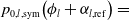
Table 1. Hybrid system properties with comparisons: n/a, and n/spec denote data not available and not relevant to be specified, respectively


Figure 1. Illustration of the case study biomimetic morphing-wing UAV. (A) Morphing degrees of freedom of the case study system: wing incidence, sweep and dihedral, all independently controllable on both wings. (B) Dogfighting context of a RaNPAS manoeuvre: the ability to significantly alter the UAV field of view, independent of the flight path. (C) An illustrative mesh of aerodynamic section models for the UAV lifting surface and fuselage.
2.0 UAV platform and modelling framework
2.1 Case study platform
As a case study, we consider the biomimetic morphing-wing UAV platform described in Ref. [Reference Pons and Cirak18], of scale c. 1 m. The platform is equipped with 6-DOF wing morphing: asymmetric sweep, dihedral and incidence. This is a maximally actuated configuration to allow significant DOFs to be identified over the course of this study. It is also equipped with a generic axial thruster for propulsion. Airframe parameters are presented in Table 1, and a scale rendering in Fig. 1A, indicating the active morphing DOFs. The platform is approximately equivalent in scale to several larger birds (e.g. the Greylag goose, Anser anser) as well as several existing morphing-wing uncrewed aerial vehicles (e.g. the NextGen MFX-1). It also is deliberately designed to be conservative: wing masses are comparatively large, to account for wing strengthening to allow high angle-of-attack manoeuvring, and lifting surface chords are comparatively small. Figure 1B illustrates a hypothetical RaNPAS manoeuvre in this platform, with applications in dogfighting UAVs, cf. [Reference Gal-Or14].
2.2 Multibody dynamic modelling framework
To model this case study UAV under strongly transient post-stall manoeuvres, we extend a previous flight dynamic modelling framework [Reference Pons and Cirak18, Reference Pons and Cirak45]. This previous framework modelled the UAV via a 12-DOF nonlinear state-space representation in the form:
 \begin{align} {{\text{B}}_{1}}\!\left( \mathbf{z},\boldsymbol{\upsilon } \right)\!\dot{\mathbf{z}}=\mathbf{f}\!\left( \mathbf{z},\boldsymbol{\upsilon } \right) -{{\text{B}}_{0}}\!\left( \mathbf{z},\boldsymbol{\upsilon } \right)\!\mathbf{z}\text{,}\end{align}
with a set of morphing and control parameters $\boldsymbol{\upsilon }$
; a state variable
$\boldsymbol{\upsilon }$
; a state variable $\mathbf{z}\in {{\mathbb{R}}^{12}}$
which encodes the reference rotational and translational positions and velocities of the system; and functionals
$\mathbf{z}\in {{\mathbb{R}}^{12}}$
which encodes the reference rotational and translational positions and velocities of the system; and functionals ${{\text{B}}_{1}}$
,
${{\text{B}}_{1}}$
, ${{\text{B}}_{0}}$
, and
${{\text{B}}_{0}}$
, and $\mathbf{f}$
describing the UAV flight dynamics. These functionals account for the multibody dynamics arising from wing morphing, under the assumption of ideal actuation–detailed definitions are given in the Supplementary material. Within
$\mathbf{f}$
describing the UAV flight dynamics. These functionals account for the multibody dynamics arising from wing morphing, under the assumption of ideal actuation–detailed definitions are given in the Supplementary material. Within $\mathbf{z}$
, the UAV’s orientation is encoded in Euler angles: the gimbal lock problem at the Euler angle pole is bypassed via a pole-switching routine, in which two alternative Euler angle parameterisations maintain non-singularity over the complete orientation space [Reference Pons46]. The aerodynamics of the UAV are modelled via a mesh of local aerodynamic section models over each of its lifting surfaces, and the fuselage (Fig. 1C). The dependency of the UAV multibody dynamic model (Equation (12)) on this local aerodynamic model,
$\mathbf{z}$
, the UAV’s orientation is encoded in Euler angles: the gimbal lock problem at the Euler angle pole is bypassed via a pole-switching routine, in which two alternative Euler angle parameterisations maintain non-singularity over the complete orientation space [Reference Pons46]. The aerodynamics of the UAV are modelled via a mesh of local aerodynamic section models over each of its lifting surfaces, and the fuselage (Fig. 1C). The dependency of the UAV multibody dynamic model (Equation (12)) on this local aerodynamic model, ${\boldsymbol{\mathcal{Q}}_{\text{A}}}\!\left( \mathbf{z},\boldsymbol{\upsilon } \right)$
, may be represented as:
${\boldsymbol{\mathcal{Q}}_{\text{A}}}\!\left( \mathbf{z},\boldsymbol{\upsilon } \right)$
, may be represented as:
 \begin{align} {{\text{B}}_{1}}\!\left( \mathbf{z},\boldsymbol{\upsilon },{\boldsymbol{\mathcal{Q}}_{\mathbf{A}}}\!\left( \mathbf{z},\boldsymbol{\upsilon } \right) \right)\!\dot{\mathbf{z}}=\mathbf{f}\!\left( \mathbf{z},\boldsymbol{\upsilon },{\boldsymbol{\mathcal{Q}}_{\mathbf{A}}}\!\left( \mathbf{z},\boldsymbol{\upsilon } \right) \right) -{{\text{B}}_{0}}\!\left( \mathbf{z},\boldsymbol{\upsilon },{\boldsymbol{\mathcal{Q}}_{\mathbf{A}}}\!\left( \mathbf{z},\boldsymbol{\upsilon } \right) \right)\!\mathbf{z}\text{.}\end{align}
2.3 Section-model aerodynamic framework
In prior work [Reference Pons and Cirak18] we developed and validated a quasisteady section-model (i.e. blade-element model) framework for the UAV aerodynamics, ${\boldsymbol{\mathcal{Q}}_{\text{A}}}\!\left( \mathbf{z},\boldsymbol{\upsilon } \right)$
, following Ananda and Selig [Reference Ananda and Selig47, Reference Selig48]. This section-model framework comprised a mesh of aerodynamic computation points (stations), with associated section models, defined across the complete UAV airframe: wings, fuselage and empennage. For each station, the kinematics of morphing and full-UAV motion together define a local flow velocity vector, which, under polar decomposition yields a local station angle-of-attack
${\boldsymbol{\mathcal{Q}}_{\text{A}}}\!\left( \mathbf{z},\boldsymbol{\upsilon } \right)$
, following Ananda and Selig [Reference Ananda and Selig47, Reference Selig48]. This section-model framework comprised a mesh of aerodynamic computation points (stations), with associated section models, defined across the complete UAV airframe: wings, fuselage and empennage. For each station, the kinematics of morphing and full-UAV motion together define a local flow velocity vector, which, under polar decomposition yields a local station angle-of-attack $\alpha$
, and airspeed vector
$\alpha$
, and airspeed vector $\mathbf{U}$
within the local aerofoil section plane. Note that no additional quasisteady corrections (e.g. in
$\mathbf{U}$
within the local aerofoil section plane. Note that no additional quasisteady corrections (e.g. in $\dot{\alpha }$
) are added to this local angle-of-attack. The spanwise component of the local flow velocity vector was neglected, thereby neglecting finite-span effects. Based on these kinematics, we compute the local station lift force (
$\dot{\alpha }$
) are added to this local angle-of-attack. The spanwise component of the local flow velocity vector was neglected, thereby neglecting finite-span effects. Based on these kinematics, we compute the local station lift force ( $\mathbf{L}$
), drag force (
$\mathbf{L}$
), drag force ( $\mathbf{D}$
), and pitching moment (
$\mathbf{D}$
), and pitching moment ( $\mathbf{M}$
) vectors, as:
$\mathbf{M}$
) vectors, as:
 \begin{align} \mathbf{L}&=\rho {{U}^{2}}{{b}_{c}}{{C}_{L}}\!\left( \alpha , \boldsymbol{\upsilon } \right)\!\overset{}{\hat{\mathbf{L}}}\,\text{,}\nonumber \\\mathbf{D}&=\rho {{U}^{2}}{{b}_{c}}{{C}_{D}}\!\left( \alpha , \boldsymbol{\upsilon } \right)\!\overset{}{\widehat{\mathbf{D}}}\,\text{,}\nonumber \\\mathbf{M}&=\rho {{U}^{2}}b_{c}^{2}{{C}_{M}}\!\left( \alpha , \boldsymbol{\upsilon } \right)\!\overset{}{\widehat{\mathbf{M}}}\,\text{,}\end{align}
via local semichord ${{b}_{c}}$
, air density
${{b}_{c}}$
, air density $\rho$
, aerodynamic coefficient functions accounting for control surface deflections
$\rho$
, aerodynamic coefficient functions accounting for control surface deflections ${{C}_{L}}\!\left( \alpha , \boldsymbol{\upsilon } \right)$
(etc.), and appropriate force unit vectors
${{C}_{L}}\!\left( \alpha , \boldsymbol{\upsilon } \right)$
(etc.), and appropriate force unit vectors $\overset{}{\hat{\mathbf{L}}}\,$
(etc.) oriented according to
$\overset{}{\hat{\mathbf{L}}}\,$
(etc.) oriented according to $\mathbf{U}$
. Aerodynamic forces and moments were then integrated across the airframe to yield
$\mathbf{U}$
. Aerodynamic forces and moments were then integrated across the airframe to yield ${\boldsymbol{\mathcal{Q}}_{\text{A}}}\!\left( \mathbf{z},\boldsymbol{\upsilon } \right)$
, and results were validated based on stability derivative data for the Pioneer RQ-2 airframe.
${\boldsymbol{\mathcal{Q}}_{\text{A}}}\!\left( \mathbf{z},\boldsymbol{\upsilon } \right)$
, and results were validated based on stability derivative data for the Pioneer RQ-2 airframe.
This prior quasisteady model is insufficient to model pitch-axis RaNPAS–as per previous studies of transient pitch-axis manoeuvrability in UAVs [Reference Mi, Zhan and Lu49, Reference Reich, Eastep, Altman and Albertani50]. For UAV flight simulation under strongly unsteady flow (local reduced frequency 0.01 $\lt \kappa \lt $
0.5), one of several higher-fidelity approaches are required: (i) fully three-dimensional computational fluid dynamics (CFD) simulations [Reference Lankford, Mayo and Chopra51, Reference Dwivedi and Damodaran52]; (ii) phenomenological dynamic stall and lift hysteresis models, such as the Goman-Khrabrov (GK) [Reference Goman and Khrabrov53] model, integrated into the section model framework [Reference Mi, Zhan and Lu49, Reference Reich, Eastep, Altman and Albertani50, Reference Wickenheiser and Garcia54–Reference Wickenheiser and Garcia56]; and (iii) model-reduction and machine-learning (ML) techniques [Reference Li, Kou and Zhang57–Reference Wang, Qian and He59]–applied to higher-fidelity data to generate an accurate surrogate aerodynamic model. In this work, we utilise a GK dynamic stall model, accounting for strongly transient effects arising from aerofoil pitching motion during the pitching manoeuvres we will study. GK models have been previously utilised in the study of other agile and morphing-wing UAVs [Reference Reich, Eastep, Altman and Albertani50, Reference Feroskhan and Go55]. In Section 3, we detail the construction of a suite of GK models for this UAV.
$\lt \kappa \lt $
0.5), one of several higher-fidelity approaches are required: (i) fully three-dimensional computational fluid dynamics (CFD) simulations [Reference Lankford, Mayo and Chopra51, Reference Dwivedi and Damodaran52]; (ii) phenomenological dynamic stall and lift hysteresis models, such as the Goman-Khrabrov (GK) [Reference Goman and Khrabrov53] model, integrated into the section model framework [Reference Mi, Zhan and Lu49, Reference Reich, Eastep, Altman and Albertani50, Reference Wickenheiser and Garcia54–Reference Wickenheiser and Garcia56]; and (iii) model-reduction and machine-learning (ML) techniques [Reference Li, Kou and Zhang57–Reference Wang, Qian and He59]–applied to higher-fidelity data to generate an accurate surrogate aerodynamic model. In this work, we utilise a GK dynamic stall model, accounting for strongly transient effects arising from aerofoil pitching motion during the pitching manoeuvres we will study. GK models have been previously utilised in the study of other agile and morphing-wing UAVs [Reference Reich, Eastep, Altman and Albertani50, Reference Feroskhan and Go55]. In Section 3, we detail the construction of a suite of GK models for this UAV.
3.0 Goman-khrabrov (GK) aerodynamic modelling
3.1 GK model formulation
To account for the transient effects of UAV pitching, we implement a novel Goman-Khrabrov (GK) model into the flight dynamic framework of Sections 2.2 and 2.3, extending both state-of-the-art GK models [Reference Mi, Zhan and Lu49, Reference Feroskhan and Go55], and the quasisteady model of this UAV [Reference Pons and Cirak18]. For each lifting surface station model within the aerodynamic mesh, the aerodynamic coefficients for force or moment $i$
(
$i$
( ${{C}_{i}}$
) as a function of effective angle-of-attack (
${{C}_{i}}$
) as a function of effective angle-of-attack ( $\alpha$
) are defined by the mixing function:
$\alpha$
) are defined by the mixing function:
 \begin{align} {{C}_{i}}\!\left( \alpha \right) =p{{C}_{i,\text{att}}}\!\left( \alpha \right)+\left( 1-p \right)\!{{C}_{i,\text{sep}}}\!\left( \alpha \right)\!\text{,}\end{align}
where ${{C}_{i,\text{att}}}\!\left( \alpha \right)$
and
${{C}_{i,\text{att}}}\!\left( \alpha \right)$
and ${{C}_{i,\text{sep}}}\!\left( \alpha \right)$
are the aerodynamic coefficient functions for hypothetical cases of local attached and separated flow, respectively. Note that Equation (4) applies independently for each lifting surface station model; but for readability we will omit indexing across each station. The three forces (
${{C}_{i,\text{sep}}}\!\left( \alpha \right)$
are the aerodynamic coefficient functions for hypothetical cases of local attached and separated flow, respectively. Note that Equation (4) applies independently for each lifting surface station model; but for readability we will omit indexing across each station. The three forces ( $i$
) of relevance are lift (
$i$
) of relevance are lift ( $L$
), drag (
$L$
), drag ( $D$
), and pitching moment (
$D$
), and pitching moment ( $M$
). Parameters
$M$
). Parameters ${{p}_{i}}$
are local dynamic mixing parameters, loosely connected to the location of the separation point along the aerofoil chord [Reference Williams, Reißner, Greenblatt, Müller-Vahl and Strangfeld60], and governed by the first-order differential equation:
${{p}_{i}}$
are local dynamic mixing parameters, loosely connected to the location of the separation point along the aerofoil chord [Reference Williams, Reißner, Greenblatt, Müller-Vahl and Strangfeld60], and governed by the first-order differential equation:
 \begin{align} {{\tau }_{1}}\dot{p}\!\left( \alpha \right) ={{p}_{0}}\!\left( \alpha -{{\tau }_{2}}\dot{\alpha } \right) -p\alpha \text{, } \end{align}
where $\alpha$
and
$\alpha$
and $\dot{\alpha }$
are the local angle-of-attack and corresponding rate;
$\dot{\alpha }$
are the local angle-of-attack and corresponding rate; ${{\tau }_{1}}$
and
${{\tau }_{1}}$
and ${{\tau }_{2}}$
are delay parameters; and
${{\tau }_{2}}$
are delay parameters; and ${{p}_{0}}\!\left( \alpha \right)$
are mixing functions representing the transition between attached and separated flow. To implement this model, we must identify the quasistatic functions
${{p}_{0}}\!\left( \alpha \right)$
are mixing functions representing the transition between attached and separated flow. To implement this model, we must identify the quasistatic functions ${{C}_{i,\text{att}}}\!\left( \alpha \right)$
,
${{C}_{i,\text{att}}}\!\left( \alpha \right)$
, ${{C}_{i,\text{sep}}}\!\left( \alpha \right)$
and
${{C}_{i,\text{sep}}}\!\left( \alpha \right)$
and ${{p}_{0}}\!\left( \alpha \right)$
and the transient delay parameters
${{p}_{0}}\!\left( \alpha \right)$
and the transient delay parameters ${{\tau }_{1}}$
and
${{\tau }_{1}}$
and ${{\tau }_{2}}$
for the case study UAV aerofoils (Table 1). The three quasistatic functions are identifiable based only on quasisteady aerodynamic coefficient data (when
${{\tau }_{2}}$
for the case study UAV aerofoils (Table 1). The three quasistatic functions are identifiable based only on quasisteady aerodynamic coefficient data (when $p = {{p}_{0}}$
), whereas the transient delay parameters are only identifiable with transient aerodynamic data.
$p = {{p}_{0}}$
), whereas the transient delay parameters are only identifiable with transient aerodynamic data.
3.2 Wing parameter identification
Quasisteady aerodynamic data for the two aerofoils (ST50W, ST50H) in the case study UAV have been previously obtained by Selig [Reference Selig61] (Fig. 2), and these data permit the identification of quasistatic GK model functions. Beginning with the wing aerofoil: nonlinear least-squares curve fitting indicates that it is poorly approximated by the flat-plate aerofoil models that are traditionally used in the GK modelling [Reference Reich, Eastep, Altman and Albertani50, Reference Wickenheiser and Garcia56], but well-approximated by extended models [Reference Williams, Reißner, Greenblatt, Müller-Vahl and Strangfeld60, Reference Williams, An, Iliev, King and Reißner62, Reference Luchtenburg, Rowley, Lohry, Martinelli and Stengel63]. For separated flow, we use:
 \begin{align} {{C}_{L,\text{sep}}}\!\left( \alpha \right)&={{a}_{L}}\,\textrm{sgn}\, \alpha \sin \!\left( {{b}_{L}}\left| \alpha +{{c}_{L}} \right|+{{d}_{L}} \right) +{{e}_{L}}\text{,}\nonumber \\{{C}_{D,\text{sep}}}\!\left( \alpha \right)&={{a}_{D}}\!\sin \!\left( {{b}_{D}}\left| \alpha \right|+{{c}_{D}} \right) +{{d}_{D}}\text{,}\nonumber \\{{C}_{M,\text{sep}}}\!\left( \alpha \right)&={{a}_{M}}\,\textrm{sgn}\, \alpha \sin \!\left( {{b}_{M}}\left| \alpha +{{c}_{M}} \right|+{{d}_{M}} \right) +{{e}_{M}}\text{,}\end{align}
for all $\alpha$
, with model parameters
$\alpha$
, with model parameters ${{a}_{i}}$
to
${{a}_{i}}$
to ${{e}_{i}}$
, and where
${{e}_{i}}$
, and where $\textrm{sgn} \cdot$
is the signum function. For attached flow, the difference in geometry between the aerofoil leading and trailing edge necessitates that we treat these edges separately:
$\textrm{sgn} \cdot$
is the signum function. For attached flow, the difference in geometry between the aerofoil leading and trailing edge necessitates that we treat these edges separately:
 \begin{align}\begin{array}{l@{\quad}l} {{C}_{L,\text{att,}l}}\!\left( {{\alpha }_{l}} \right) ={{C}_{L\alpha ,l}}{{\alpha }_{l}}\text{,} & {{C}_{L,\text{att,}t}}\!\left( {{\alpha }_{t}} \right) ={{C}_{L\alpha ,t}}{{\alpha }_{t}}\text{,} \\{{C}_{M,\text{att,}l}}\!\left( {{\alpha }_{l}} \right) =0\text{,} & {{C}_{M,\text{att,}t}}\!\left( {{\alpha }_{t}} \right) ={{C}_{M\alpha ,t}}{{\alpha }_{t}}\text{,} \\{{C}_{D,\text{att,}l}}\!\left( {{\alpha }_{l}} \right) =0\text{,} & {C_{D,{\textrm{att,}}t}} \!\left( {{\alpha _t}} \right) = 0, \end{array} \end{align}
where ${\alpha _l}$
and
${\alpha _l}$
and ${\alpha _t}$
are the leading and trailing edge angles of attack, representing a partition of the full domain,
${\alpha _t}$
are the leading and trailing edge angles of attack, representing a partition of the full domain, $\left| \alpha \right| \lt $
180
$\left| \alpha \right| \lt $
180 $^\circ $
, into
$^\circ $
, into $\left| \alpha \right| \le $
90
$\left| \alpha \right| \le $
90 $^\circ $
and
$^\circ $
and $\left| {\left| \alpha \right| - {\textrm{180}}^\circ } \right| \le $
. 90
$\left| {\left| \alpha \right| - {\textrm{180}}^\circ } \right| \le $
. 90 $^\circ $
, the latter of which is mapped back to
$^\circ $
, the latter of which is mapped back to $\left| \alpha \right| \le $
90
$\left| \alpha \right| \le $
90 $^\circ $
again. Three of the attached flow models are observably zero (Equation (7), Fig. 2). The effect of aileron deflection is not considered, as this control function will be achieved by incidence morphing.
$^\circ $
again. Three of the attached flow models are observably zero (Equation (7), Fig. 2). The effect of aileron deflection is not considered, as this control function will be achieved by incidence morphing.

Figure 2. Quasisteady aerodynamic coefficient data for the wing aerofoil (ST50W), as a function of angle-of-attack ( $\alpha $
), reconstructed from the quasistatic GK attached and separated flow models, compared to the original semi-empirical data [Reference Selig61].
$\alpha $
), reconstructed from the quasistatic GK attached and separated flow models, compared to the original semi-empirical data [Reference Selig61].
Model parameters for Equations (6) and (7) are identified via a nonlinear least-squares approach applied to selections of clearly attached and separated flow. Data-driven estimates of ${p_0}$
can then be obtained by solving
${p_0}$
can then be obtained by solving $p = {p_0}$
in Equation (4) using aerodynamic source data. Figure 3 shows the results of this process: for the leading edge (
$p = {p_0}$
in Equation (4) using aerodynamic source data. Figure 3 shows the results of this process: for the leading edge ( ${\alpha _l}$
), compared to the compared to a traditional arctangent expression for
${\alpha _l}$
), compared to the compared to a traditional arctangent expression for ${p_0}\!\left( \alpha \right)$
, as per Wickenheiser and Garcia [Reference Wickenheiser and Garcia56] and Reich et al. [Reference Reich, Eastep, Altman and Albertani50]:
${p_0}\!\left( \alpha \right)$
, as per Wickenheiser and Garcia [Reference Wickenheiser and Garcia56] and Reich et al. [Reference Reich, Eastep, Altman and Albertani50]:
 \begin{align} {p_{0,l}}\!\left( {{\alpha _l}} \right) = \left\{\begin{array}{c@{\quad}c}1 & {}{\left| {{\alpha _l}} \right| \lt 7^\circ } \\{ - 0.3326\,{{\tan }^{ - 1}}\!\left( {\left| {{\alpha _l}} \right| + 16} \right) + 0.5} & {}{7^\circ \le \left| {{\alpha _l}} \right| \le 37^\circ } \\0 & {}{\left| {{\alpha _l}} \right| \gt 37^\circ .}\end{array} \right.\end{align}


Note that ${\tan ^{ - 1}}\!\left( \cdot \right)$
is here taken to output a value in radians. For the trailing edge, we modify this expression to account for earlier and faster separation:
${\tan ^{ - 1}}\!\left( \cdot \right)$
is here taken to output a value in radians. For the trailing edge, we modify this expression to account for earlier and faster separation:
 \begin{align} {p_{0,t}}\!\left( {{\alpha _t}} \right) = \left\{ \begin{array}{c@{\quad}c}1 {}& {\left| {{\alpha _t}} \right| \lt 4^\circ } \\{ - 0.3326\,{{\tan }^{ - 1}}\!\left( {1.6\left| {{\alpha _t}} \right| + 16} \right) + 0.5} & {}{4^\circ \le \left| {{\alpha _t}} \right| \le 21^\circ } \\0 & {}{\left| {{\alpha _t}} \right| \gt 21^\circ .}\end{array} \right.\end{align}
Quasisteady aerodynamic coefficient data for the ST50W wing may then be reconstructed for comparison. Figure 2 shows this data alongside the GK reconstruction using the arctangent ${p_0}$
(Equations (8) and (9). The result is overall very good: the separated and attached flow regimes are modelled well. Discrepancies are observed in trailing edge transition in drag and moment coefficients: as can be seen in Fig. 3, trailing edge drag and moment appear to behave according to different
${p_0}$
(Equations (8) and (9). The result is overall very good: the separated and attached flow regimes are modelled well. Discrepancies are observed in trailing edge transition in drag and moment coefficients: as can be seen in Fig. 3, trailing edge drag and moment appear to behave according to different ${p_0}\!\left( \alpha \right)$
functions. However, defining three independent mixing functions would be overfitting these data, and would break the physical interpretability of
${p_0}\!\left( \alpha \right)$
functions. However, defining three independent mixing functions would be overfitting these data, and would break the physical interpretability of $p$
as a mixing parameter.
$p$
as a mixing parameter.
3.3 Stabiliser parameter identification
The aerodynamic data for the stabiliser aerofoil (ST50H) [Reference Selig61], is dependent on the stabiliser control surface (elevator/rudder) deflection. To begin, we assume that control-surface motion can be modelled quasistatically (i.e. that this motion induces no flow). The dataset from Selig [Reference Selig61] contains aerodynamic coefficient data at seven different elevator deflections ( $ - $
50
$ - $
50 $^\circ $
,
$^\circ $
, $ - $
30
$ - $
30 $^\circ $
,
$^\circ $
, $ - $
15
$ - $
15 $^\circ $
, 0
$^\circ $
, 0 $^\circ $
, 15
$^\circ $
, 15 $^\circ $
, 30
$^\circ $
, 30 $^\circ $
, 50
$^\circ $
, 50 $^\circ $
); but only four are unique (e.g.
$^\circ $
); but only four are unique (e.g. ${\beta _e} \in \!\left[ { - {\textrm{50}},\;{\textrm{0}}} \right]{{^\circ }}$
) due to the symmetric aerofoil profile: downwards aerofoil motion at downwards control surface deflection is equivalent to upwards motion at upwards deflection. For each element of the unique set
${\beta _e} \in \!\left[ { - {\textrm{50}},\;{\textrm{0}}} \right]{{^\circ }}$
) due to the symmetric aerofoil profile: downwards aerofoil motion at downwards control surface deflection is equivalent to upwards motion at upwards deflection. For each element of the unique set ${\beta _e} \in \!\left[ { - {\textrm{50}},\;{\textrm{0}}} \right]{{^\circ }}$
, we identify separated flow models of the form:
${\beta _e} \in \!\left[ { - {\textrm{50}},\;{\textrm{0}}} \right]{{^\circ }}$
, we identify separated flow models of the form:
 \begin{align} {C_{L,{\textrm{sep}}}}\!\left( \alpha \right) &= {a_L}\,{\mathop{\textrm{sgn}}} \!\left( {\alpha + {c_L}} \right)\!\sin \!\left( {{b_L}\left| {\alpha + {c_L}} \right| + {d_L}} \right) + {e_L}{\textrm{,}}\nonumber \\{C_{D,{\textrm{sep}}}}\!\left( \alpha \right) &= \left\{ {\begin{array}{c@{\quad}c}{{a_D}\cos \!\left( {{b_D}\left| {\alpha + {c_D}} \right| + {d_D}} \right) + {e_D}{\textrm{,}}} & {}{{\beta _e} = 0}\\{{a_D}\sin \!\left( {{b_D}\alpha + {c_D}} \right) + {d_D}{\textrm{,}}} & {}{{\textrm{o}}{\textrm{.w}}{\textrm{.,}}}\end{array}} \right. \nonumber \\{C_{M,{\textrm{sep}}}}\!\left( \alpha \right) &= {a_M}\,{\mathop{\textrm{sgn}}} \!\left( {\alpha + {c_M}} \right)\!\sin \!\left( {{b_M}\left| {\alpha + {c_M}} \right| + {d_M}} \right) + {e_M}{\textrm{,}}\end{align}
and attached-flow models as per Equation (7). The key difference between stabiliser (Equation (10)) and wing (Equation (6)) models is the simpler sinusoid drag model for the stabiliser at nonzero ${\beta _e}$
: the complexity of the coefficient data does not permit identification of more complex models. We use a nonlinear least-squares approach to identify model parameters for Equation (7) across the unique
${\beta _e}$
: the complexity of the coefficient data does not permit identification of more complex models. We use a nonlinear least-squares approach to identify model parameters for Equation (7) across the unique ${\beta _e}$
. This identification is fully automated except for a manual indication of the location of areas of attached and separated flow for identification. The Supplementary Material presents the four unique identified models in each aerodynamic coefficient.
${\beta _e}$
. This identification is fully automated except for a manual indication of the location of areas of attached and separated flow for identification. The Supplementary Material presents the four unique identified models in each aerodynamic coefficient.
We then identify the mixing parameter functions, ${p_0}\!\left( \alpha \right)$
. Figure 4 shows data-driven estimates of
${p_0}\!\left( \alpha \right)$
. Figure 4 shows data-driven estimates of ${p_0}\!\left( \alpha \right)$
obtained by solving Equation (4) for
${p_0}\!\left( \alpha \right)$
obtained by solving Equation (4) for $p = {p_0}$
in the vicinity of transition. Estimates are available for
$p = {p_0}$
in the vicinity of transition. Estimates are available for ${C_L}$
at the leading and trailing edge, and
${C_L}$
at the leading and trailing edge, and ${C_M}$
at the trailing edge–areas where the attached flow model is nonzero. In Fig. 4, these estimates are presented with respect to the reference angles of attack,
${C_M}$
at the trailing edge–areas where the attached flow model is nonzero. In Fig. 4, these estimates are presented with respect to the reference angles of attack, ${\alpha _{l,{\textrm{ref}}}}$
and
${\alpha _{l,{\textrm{ref}}}}$
and ${\alpha _{t,{\textrm{ref}}}}$
: these values are the centre-points of the attached flow regions, specified manually, and nonzero for nonzero
${\alpha _{t,{\textrm{ref}}}}$
: these values are the centre-points of the attached flow regions, specified manually, and nonzero for nonzero ${\beta _e}$
. A notable feature of these results is their asymmetry, with long tails at negative
${\beta _e}$
. A notable feature of these results is their asymmetry, with long tails at negative $\alpha $
(for
$\alpha $
(for ${\beta _e} \lt $
0). This is likely a physical effect. At positive
${\beta _e} \lt $
0). This is likely a physical effect. At positive $\alpha $
values (for
$\alpha $
values (for $_e \lt $
0), large stall peaks are observed, whereas at negative
$_e \lt $
0), large stall peaks are observed, whereas at negative $\alpha $
there is a flat plateau: physically, this could arise from flow reattachment effects when both the control surface and the aerofoil are inclined upwards (
$\alpha $
there is a flat plateau: physically, this could arise from flow reattachment effects when both the control surface and the aerofoil are inclined upwards ( ${\beta _e} \lt $
0,
${\beta _e} \lt $
0, $\alpha \gt $
0), leading to a state in which the control surface is itself at lower angle-of-attack. The arctangent sigmoid used in previous GK models [Reference Reich, Eastep, Altman and Albertani50] cannot capture this asymmetry. In its place we propose a new GK sigmoid function, based on the logistic function. Its symmetric form, for the leading edge (
$\alpha \gt $
0), leading to a state in which the control surface is itself at lower angle-of-attack. The arctangent sigmoid used in previous GK models [Reference Reich, Eastep, Altman and Albertani50] cannot capture this asymmetry. In its place we propose a new GK sigmoid function, based on the logistic function. Its symmetric form, for the leading edge ( ${\alpha _l}$
), is:
${\alpha _l}$
), is:
 \begin{align} {p_{0,l,{\textrm{sym}}}}\!\left( {{\alpha _l}} \right) = S\!\left( {\frac{1}{{{m_l}}}\!\left( {\left| {{\alpha _l} - {\alpha _{l,{\textrm{ref}}}}} \right| - {\phi _l}} \right)\!} \right)\!{\textrm{, }}S\!\left( x \right) = \frac{1}{{1 + \exp \!\left( x \right)\!}}{\textrm{,}}\end{align}
where $S\!\left( x \right)$
is the logistic function and
$S\!\left( x \right)$
is the logistic function and ${\alpha _{l,{\textrm{ref}}}}$
is the centre point of the attached flow region (specified manually). The shift parameter
${\alpha _{l,{\textrm{ref}}}}$
is the centre point of the attached flow region (specified manually). The shift parameter ${\phi _l}$
is the location of the halfway point, i.e.
${\phi _l}$
is the location of the halfway point, i.e. ${p_{0,l,{\textrm{sym}}}}\!\left( {{\phi _l} + {\alpha _{l,{\textrm{ref}}}}} \right) = $
0.5. The width parameter
${p_{0,l,{\textrm{sym}}}}\!\left( {{\phi _l} + {\alpha _{l,{\textrm{ref}}}}} \right) = $
0.5. The width parameter ${m_l}$
governs the gradient at this point. The interpretable nature of these parameters is an aid to identification. To account for asymmetry in angle-of-attack, we add a one-sided Gaussian term to Equation (11), yielding the completed
${m_l}$
governs the gradient at this point. The interpretable nature of these parameters is an aid to identification. To account for asymmetry in angle-of-attack, we add a one-sided Gaussian term to Equation (11), yielding the completed ${p_{0,l}}$
:
${p_{0,l}}$
:
 \begin{align} {p_{0,l}}\!\left( {{\alpha _l}} \right) &= \left( {1 - {p_{0,{\textrm{sym}}}}\!\left( {{\alpha _l}} \right)} \right)\!G\!\left( {{\alpha _l}} \right) + {p_{0,i,{\textrm{sym}}}}\!\left( {{\alpha _l}} \right)\!{\textrm{,}}\nonumber \\G\!\left( {{\alpha _l}} \right) &= {M_l}\exp \!\left( { - {{\left( {\frac{{{\alpha _l} - {\alpha _{l,{\textrm{ref}}}} + {\phi _l}}}{{{w_l}}}} \right)\!}^2}} \right)\!{\left[ {{\alpha _l} - {\alpha _{l,{\textrm{ref}}}} \lt 0} \right]_{{\textrm{IV}}}}{\textrm{,}}\end{align}
where ${w_l}$
governs the width of the one-sided Gaussian function, and the parameter
${w_l}$
governs the width of the one-sided Gaussian function, and the parameter ${M_l}$
its height.
${M_l}$
its height. ${\phi _l}$
is the parameter identified in Equation (11), and
${\phi _l}$
is the parameter identified in Equation (11), and ${\!\left[ \cdot \right]_{{\textrm{IV}}}}$
is the Iverson bracket [Reference Graham, Knuth and Patashnik64], such that
${\!\left[ \cdot \right]_{{\textrm{IV}}}}$
is the Iverson bracket [Reference Graham, Knuth and Patashnik64], such that ${\!\left[ s \right]_{{\textrm{IV}}}} = $
1 if
${\!\left[ s \right]_{{\textrm{IV}}}} = $
1 if $s$
is true, and
$s$
is true, and ${\!\left[ s \right]_{{\textrm{IV}}}} = $
0 if
${\!\left[ s \right]_{{\textrm{IV}}}} = $
0 if $s$
is false. This addition maintains smoothness (
$s$
is false. This addition maintains smoothness ( ${C^\infty }$
) over the halfspaces
${C^\infty }$
) over the halfspaces ${\alpha _l} \gt {\alpha _{l,{\textrm{ref}}}}$
and
${\alpha _l} \gt {\alpha _{l,{\textrm{ref}}}}$
and ${\alpha _l} \lt {\alpha _{l,{\textrm{ref}}}}$
.
${\alpha _l} \lt {\alpha _{l,{\textrm{ref}}}}$
.

Figure 4. Unfiltered approximations to ${p_0}\!\left( \alpha \right)$
derived from stabiliser aerofoil (ST50H) leading edge (L.E.) and trailing edge (T.E.) aerodynamic data, against the associated logistic sigmoid fit.
${p_0}\!\left( \alpha \right)$
derived from stabiliser aerofoil (ST50H) leading edge (L.E.) and trailing edge (T.E.) aerodynamic data, against the associated logistic sigmoid fit.
Table 2. Fitted model parameters for the logistic ${p_0}$
functions
${p_0}$
functions


Figure 5. Quasisteady aerodynamic coefficient data for the stabiliser aerofoil (ST50H), as a function of both angle-of-attack ( $\alpha $
) and control surface deflection (
$\alpha $
) and control surface deflection ( ${\beta _e}$
), reconstructed from the quasistatic GK attached and separated flow models, and compared to the original data.
${\beta _e}$
), reconstructed from the quasistatic GK attached and separated flow models, and compared to the original data.
In the case of the trailing edge ( ${\alpha _t}$
), discrepancy between the empirical
${\alpha _t}$
), discrepancy between the empirical ${p_0}$
estimates computed from
${p_0}$
estimates computed from ${C_L}$
and
${C_L}$
and ${C_M}$
precludes identification of an asymmetric
${C_M}$
precludes identification of an asymmetric ${p_{0,t}}$
. We instead use the same symmetric form as in Equation (11), with parameters
${p_{0,t}}$
. We instead use the same symmetric form as in Equation (11), with parameters ${m_t}$
and
${m_t}$
and ${\phi _t}$
:
${\phi _t}$
:
 \begin{align} {p_{0,t,{\textrm{sym}}}}\!\left( {{\alpha _t}} \right) = S\!\left( {\frac{1}{{{m_t}}}\!\left( {\left| {{\alpha _t} - {\alpha _{t,{\textrm{ref}}}}} \right| - {\phi _t}} \right)\!} \right)\!{\textrm{,}}\end{align}
For identification, all ${p_0}$
parameters (for both leading and trailing edge) are manually estimated for
${p_0}$
parameters (for both leading and trailing edge) are manually estimated for ${\beta _e} = $ $ - $
50° and
$ - $
50° and ${\beta _e} = $
0°; and models at the internal surface-deflection points are generated by linear interpolation. Table 2 shows the identified parameters, including the interpolation index (
${\beta _e} = $
0°; and models at the internal surface-deflection points are generated by linear interpolation. Table 2 shows the identified parameters, including the interpolation index ( $k \in \!\left[ {{\textrm{0, 1}}} \right]$
for
$k \in \!\left[ {{\textrm{0, 1}}} \right]$
for ${\beta _e} \in \!\left[ { - {\textrm{50}},\;{\textrm{0}}} \right]{{^\circ }}$
), and Fig. 4 the identified
${\beta _e} \in \!\left[ { - {\textrm{50}},\;{\textrm{0}}} \right]{{^\circ }}$
), and Fig. 4 the identified ${p_0}\!\left( \alpha \right)$
functions. The parameter interpolation is linear and two-point (
${p_0}\!\left( \alpha \right)$
functions. The parameter interpolation is linear and two-point ( $k \in \!\left\{ {{\textrm{0, 1}}} \right\}$
), with the exception of
$k \in \!\left\{ {{\textrm{0, 1}}} \right\}$
), with the exception of ${M_l}$
, which shows a rising trend with
${M_l}$
, which shows a rising trend with $k$
but must be zero at
$k$
but must be zero at $k = $
1 to preserve symmetry. To account for this effect, we use a non-monotonic piecewise-linear profile (Table 2). For both edges, the complete set of identified models can be extended to
$k = $
1 to preserve symmetry. To account for this effect, we use a non-monotonic piecewise-linear profile (Table 2). For both edges, the complete set of identified models can be extended to ${\beta _e} \gt $
0 by symmetry, and estimated quasisteady coefficient profiles can be reconstructed using the relevant sigmoid
${\beta _e} \gt $
0 by symmetry, and estimated quasisteady coefficient profiles can be reconstructed using the relevant sigmoid ${p_0}$
expressions and the separated- and attached-flow models. Figure 5 shows the GK reconstruction of the ST50H quasisteady aerodynamic coefficients as a function of elevator deflection and
${p_0}$
expressions and the separated- and attached-flow models. Figure 5 shows the GK reconstruction of the ST50H quasisteady aerodynamic coefficients as a function of elevator deflection and $\alpha $
, compared with the original results of Selig [Reference Selig61]. As can be seen, a good agreement is observed, despite some variation in the laminar-turbulent transition zones. The primary limitations of the model remain the discrepancy in identified separation point between the lift and moment coefficient data.
$\alpha $
, compared with the original results of Selig [Reference Selig61]. As can be seen, a good agreement is observed, despite some variation in the laminar-turbulent transition zones. The primary limitations of the model remain the discrepancy in identified separation point between the lift and moment coefficient data.
3.4 Transient delay parameter identification
With the quasistatic components of the GK models for both UAV aerofoils fully identified, the remaining task is to identify the transient delay parameters ${\tau _1}$
and
${\tau _1}$
and ${\tau _2}$
. For comparison, Table 3 presents a range of delay parameters identified in the literature for several aerofoils. The variation across reported values is large: e.g. for the NACA0009 factor of 2 variation (in
${\tau _2}$
. For comparison, Table 3 presents a range of delay parameters identified in the literature for several aerofoils. The variation across reported values is large: e.g. for the NACA0009 factor of 2 variation (in ${\tau _2}$
) is observed, and for the NACA0018 a factor of 7 (in
${\tau _2}$
) is observed, and for the NACA0018 a factor of 7 (in ${\tau _1}$
). These results indicate that a precise identification of the delay parameters is sensitive to the dataset–contributing factors could include wind-tunnel/wall effects, surface roughness and CFD modelling choices. Additionally, this is consistent with the observation that these delay parameters determine the aerofoil behaviour in the laminar-turbulent transition, including the case of attached flow at angles of attack below quasisteady stall: both factors are sensitive to modelling and dataset specifics. Note also that, while data remains sparse, GK models can in theory account for a range of motions that lead to dynamic stall: not only pure pitching motion, but pure plunging [Reference Chiereghin, Cleaver and Gursul66] and gust encounters [Reference Sedky, Jones and Lagor67]. Identified delay values for NACA0012 under these latter conditions is included in Table 3. Recently progress has been made on unifying and generalising GK-type models [Reference Ayancik and Mulleners72], but the complete range of variation in identified delay values across the literature remains unexplained.
${\tau _1}$
). These results indicate that a precise identification of the delay parameters is sensitive to the dataset–contributing factors could include wind-tunnel/wall effects, surface roughness and CFD modelling choices. Additionally, this is consistent with the observation that these delay parameters determine the aerofoil behaviour in the laminar-turbulent transition, including the case of attached flow at angles of attack below quasisteady stall: both factors are sensitive to modelling and dataset specifics. Note also that, while data remains sparse, GK models can in theory account for a range of motions that lead to dynamic stall: not only pure pitching motion, but pure plunging [Reference Chiereghin, Cleaver and Gursul66] and gust encounters [Reference Sedky, Jones and Lagor67]. Identified delay values for NACA0012 under these latter conditions is included in Table 3. Recently progress has been made on unifying and generalising GK-type models [Reference Ayancik and Mulleners72], but the complete range of variation in identified delay values across the literature remains unexplained.
Table 3. GK delay parameters reported in the literature; conditions are for pitching motion unless otherwise noted

In addition, CFD simulations of the ST50W aerofoil are described in Ref. (Reference Pons46). From Table 3–in particular, NACA0009–and these CFD simulations, we estimate ${\tau _1} = {\tau _2} = $
2.3
${\tau _1} = {\tau _2} = $
2.3 ${c_c}/U$
. Two upper bounds on this estimate, in terms of motion transience, are defined. The maximum permissible reduced frequency is
${c_c}/U$
. Two upper bounds on this estimate, in terms of motion transience, are defined. The maximum permissible reduced frequency is $\kappa = {b_c}{{\Omega }}/U = $
0.5, where
$\kappa = {b_c}{{\Omega }}/U = $
0.5, where ${b_c}$
is the local section semichord, and
${b_c}$
is the local section semichord, and ${{\Omega }}$
is the frequency (in rad/s) of aerofoil motion. The maximum permissible reduced pitch rate is
${{\Omega }}$
is the frequency (in rad/s) of aerofoil motion. The maximum permissible reduced pitch rate is $r = {b_c}\dot \alpha /U = $
0.13, where
$r = {b_c}\dot \alpha /U = $
0.13, where $\dot \alpha $
is the local section pitch rate. Beyond these two limits, aerodynamic added mass becomes significant, and this is not accounted for in the GK model. Based on the reported range of Reynolds numbers (Re) over which GK models have been developed, we estimate Re
$\dot \alpha $
is the local section pitch rate. Beyond these two limits, aerodynamic added mass becomes significant, and this is not accounted for in the GK model. Based on the reported range of Reynolds numbers (Re) over which GK models have been developed, we estimate Re $ = U{c_c}/\nu = $ ${\textrm{1}}{{\textrm{0}}^{\textrm{6}}}$
as maximum permissible Reynolds number. Practically, to retain GK model validity, this limits the UAV airspeed to below 100 m/s; and, for more common manoeuvres at airspeed 40 m/s, the UAV pitch rate
${\textrm{1}}{{\textrm{0}}^{\textrm{6}}}$
as maximum permissible Reynolds number. Practically, to retain GK model validity, this limits the UAV airspeed to below 100 m/s; and, for more common manoeuvres at airspeed 40 m/s, the UAV pitch rate $\dot \alpha $
to 70 rad/s. In Section 6 we will assess simulated manoeuvres against these validity limits in reduced pitch rate and reduced frequency. We note also that there are several open questions with regard to how to integrate GK dynamic stall models into a flight simulation context [Reference Pons46]: most significantly, exactly how the delay parameters should be taken to scale with local station airspeed (
$\dot \alpha $
to 70 rad/s. In Section 6 we will assess simulated manoeuvres against these validity limits in reduced pitch rate and reduced frequency. We note also that there are several open questions with regard to how to integrate GK dynamic stall models into a flight simulation context [Reference Pons46]: most significantly, exactly how the delay parameters should be taken to scale with local station airspeed ( $U$
), given that this airspeed will vary. We take these delay parameters to scale with
$U$
), given that this airspeed will vary. We take these delay parameters to scale with $U$
, according to the dimensional relation
$U$
, according to the dimensional relation ${\tau _1} = {\tau _2} = $
2.3
${\tau _1} = {\tau _2} = $
2.3 ${c_c}/U$
, but further research is required to establish this relationship with confidence.
${c_c}/U$
, but further research is required to establish this relationship with confidence.
3.5 Combined multibody-GK model framework
The completed GK model defines the aerodynamic force function ${{\boldsymbol{\mathcal{Q}}}_{\textrm{A}}}\!\left( {{\textrm{z}},{{\upsilon }}} \right)$
in the system dynamics (Equation (2)). The combination of GK and multibody-dynamic models for the case-study UAV led to the nonlinear state-space model:
${{\boldsymbol{\mathcal{Q}}}_{\textrm{A}}}\!\left( {{\textrm{z}},{{\upsilon }}} \right)$
in the system dynamics (Equation (2)). The combination of GK and multibody-dynamic models for the case-study UAV led to the nonlinear state-space model:
 \begin{align} \!\left[ {\begin{array}{l@{\quad}l}{{{\bf{B}}_1}\!\left( {{\bf{z}},{\boldsymbol{\upsilon }}} \right)\!} & {}\\ & {}{{{\textrm{T}}_1}\!\left( {{\bf{z}},{\boldsymbol{\upsilon }}} \right)\!}\end{array}} \right]\!\left[ {\begin{array}{c}{{\dot{\bf z}}}\\{{\dot{\bf p}}}\end{array}} \right] = \left[ {\begin{array}{c}{{\bf{f}}\!\left( {{\bf{z}},{\bf{p}},{\boldsymbol{\upsilon }}} \right)\!}\\{{\boldsymbol{p}_0}\!\left( {{\boldsymbol{\alpha }}\!\left( {{\bf{z}},{\boldsymbol{\upsilon }}} \right) - {{\textrm{T}}_2}\!\left( {{\bf{z}},{\boldsymbol{\upsilon }}} \right)\!{\dot{\bf \alpha }}\!\left( {{\bf{z}},{\boldsymbol{\upsilon }}} \right)\!} \right)\!}\end{array}} \right] + \left[ {\begin{array}{l@{\quad}l}{ - {{\textrm{B}}_0}\!\left( {{\bf{z}},{\boldsymbol{\upsilon }}} \right)\!} {}& \\ & {}{\textrm{I}}\end{array}} \right]\!\left[ {\begin{array}{c}{\bf{z}}\\{\bf{p}}\end{array}} \right],\end{align}
where the terms in ${\bf{p}}$
and
${\bf{p}}$
and ${\dot{\bf p}}$
represent the flow attachment dynamics (Equation (5)) over all lifting surfaces (
${\dot{\bf p}}$
represent the flow attachment dynamics (Equation (5)) over all lifting surfaces ( $p$
now becoming
$p$
now becoming ${p_j}$
for mesh station
${p_j}$
for mesh station $j$
), and the terms in
$j$
), and the terms in ${\bf{z}}$
and
${\bf{z}}$
and ${\dot{\bf z}}$
represent the UAV multibody dynamics (Equation (2)). The addition of the flow attachment dynamics significantly increases the size of the state space. In Section 4.4 we perform a mesh convergence study over a relevant manoeuvre trajectory to determine an appropriate mesh resolution for the lifting surface aerodynamic stations.
${\dot{\bf z}}$
represent the UAV multibody dynamics (Equation (2)). The addition of the flow attachment dynamics significantly increases the size of the state space. In Section 4.4 we perform a mesh convergence study over a relevant manoeuvre trajectory to determine an appropriate mesh resolution for the lifting surface aerodynamic stations.

Figure 6. Comparison of GK model predictions with CFD data for a swept wing of finite span, NACA0012 aerofoil, from Hammer et al. [Reference Hammer, Garmann and Visbal73]. A scale render shows the swept wing, matching the aspect ratio (AR) = 4 geometry reported by Hammer et al. [Reference Hammer, Garmann and Visbal73], alongside histories of the wing lift coefficient, wing drag coefficient, and wing pitching moment coefficient about the local quarter-chord. The GK model consistently overpredicts the strength of hysteresis in the aerodynamic profiles–providing a bound on the strength of hysteresis in the case-study UAV.
3.6 Comparison with CFD data for a swept wing of finite span
The completed state-space model (Equation (15)) integrates GK modelling with wing morphing about multiple axes–including in sweep and dihedral. Previous GK-based flight dynamic models have not considered these morphing axes [Reference Feroskhan and Go55, Reference Wickenheiser and Garcia56]. To study the fidelity of GK modelling under sweep morphing, we compare GK model predictions with the CFD results of Hammer et al. [Reference Hammer, Garmann and Visbal73] for a NACA0012 30° swept wing of finite span undergoing dynamic stall. The wing planform is illustrated in Fig. 6. Hammer et al. [Reference Hammer, Garmann and Visbal73] prescribe incidence motion:
 \begin{align} \theta \!\left( t \right) = {\theta _0} + {{\Delta }}\theta \!\left( {1 - \cos \!\left( {\frac{{2\kappa Ut}}{{{c_{{\textrm{swept}}}}}}} \right)\!} \right)\!{\textrm{,}}\end{align}
for minimum incidence angle ${\theta _0} = $
4°, incidence amplitude
${\theta _0} = $
4°, incidence amplitude ${{\Delta }}\theta = $
9°, reduced frequency
${{\Delta }}\theta = $
9°, reduced frequency $\kappa = \pi /{\textrm{16}}$
, airspeed
$\kappa = \pi /{\textrm{16}}$
, airspeed $U$
, and swept-wing chord
$U$
, and swept-wing chord ${c_{{\textrm{swept}}}}$
. From Equation (13) we infer that the angular frequency of pitching oscillation is
${c_{{\textrm{swept}}}}$
. From Equation (13) we infer that the angular frequency of pitching oscillation is ${{\Omega }} = 2\kappa U/{c_{{\textrm{swept}}}} = \pi U/8{c_{{\textrm{swept}}}}$
, which we match to an arbitrary dimensional wing scale, since our GK model has no Reynolds number dependence. Figure 6 compares CFD and GK model predictions in wing lift, drag and moment coefficient (with reference area
${{\Omega }} = 2\kappa U/{c_{{\textrm{swept}}}} = \pi U/8{c_{{\textrm{swept}}}}$
, which we match to an arbitrary dimensional wing scale, since our GK model has no Reynolds number dependence. Figure 6 compares CFD and GK model predictions in wing lift, drag and moment coefficient (with reference area ${c_{{\textrm{swept}}}} \times $
wingspan, and reference chord
${c_{{\textrm{swept}}}} \times $
wingspan, and reference chord ${c_{{\textrm{swept}}}}$
). Several notable features are observed–with the caveat that the NACA0012 and ST50W aerofoils differ.
${c_{{\textrm{swept}}}}$
). Several notable features are observed–with the caveat that the NACA0012 and ST50W aerofoils differ.
First, the GK model generally overpredicts the strength of hysteresis in the aerodynamic coefficients. The peak lift coefficient is predicted relatively well, though the earlier timing of this peak leads to a wider hysteresis loop. This overprediction reflects the choice of delay parameters ( ${\tau _1}$
and
${\tau _1}$
and ${\tau _2}$
, which, as per Section 3.4, are sensitive) and provides a useful bound on the real hysteresis strength in the case study UAV. That is, by comparing simulation results between the GK model and quasistatic model, we can be assured that realistic behaviour lies between these two simulation extremes. Second, the GK model predicts a region of negative drag, due partly to thrust forces from the pitching-induced changes in angle-of-attack. These thrust forces are not necessarily non-physical–as regions of negative drag are observed in certain dynamic stall conditions [Reference Kerho74–Reference Weaver, McAlister and Tso76]–though they do not occur in the dataset of Hammer et al. [Reference Hammer, Garmann and Visbal73]. This suggests that future refinement of GK drag modelling (Fig. 2) is in order.
${\tau _2}$
, which, as per Section 3.4, are sensitive) and provides a useful bound on the real hysteresis strength in the case study UAV. That is, by comparing simulation results between the GK model and quasistatic model, we can be assured that realistic behaviour lies between these two simulation extremes. Second, the GK model predicts a region of negative drag, due partly to thrust forces from the pitching-induced changes in angle-of-attack. These thrust forces are not necessarily non-physical–as regions of negative drag are observed in certain dynamic stall conditions [Reference Kerho74–Reference Weaver, McAlister and Tso76]–though they do not occur in the dataset of Hammer et al. [Reference Hammer, Garmann and Visbal73]. This suggests that future refinement of GK drag modelling (Fig. 2) is in order.
4.0 Classical RaNPAS capabilities
4.1 Open-loop control of nonlinear longitudinal stability
Gal-Or’s [Reference Gal-Or14] classification of rapid nose-pointing-and-shooting (RaNPAS) capability includes the supermanoeuvre commonly referred to as the cobra. This is a pitch-axis supermanoeuvre which involves tilting the UAV backwards from level flight to beyond 90° pitch angle, and then forwards to level flight again, while maintaining approximately constant altitude [Reference Ericsson17]. At a minimum, generating a cobra manoeuvre via open-loop wing morphing requires at least three morphing configurations: (1) an initial trim configuration; (2) a configuration to generate the moment required to pitch the UAV up to the partially inverted position; and (3) a configuration to pitch the UAV down from the partially inverted position, and back to trim. The initial trim configuration (1) is computable via existing trimming methods [Reference Pons and Cirak18]. However, identifying candidates for configurations (2) and (3) is challenging, given the large configuration space. To identify these candidates, we develop a novel strategy based on optimisation of the UAV’s nonlinear longitudinal stability, as follows.

Figure 7. Static longitudinal stability profile of several candidate pitch-up configurations: (A) with all morphing DOF enabled; (B) with only sweep ( ${{\Lambda }}$
) and incidence (
${{\Lambda }}$
) and incidence ( $\alpha $
) DOF enabled; (C) with only the incidence DOF enabled. The key feature of these profiles is the degree to which a positive (upwards) pitch acceleration is maintained at high angles of attack: the longer a positive acceleration is maintained, the greater the maximum attainable angle-of-attack during a RaNPAS manoeuvre. For each configuration, the airframe is rendered at a constant representative high angle-of-attack.
$\alpha $
) DOF enabled; (C) with only the incidence DOF enabled. The key feature of these profiles is the degree to which a positive (upwards) pitch acceleration is maintained at high angles of attack: the longer a positive acceleration is maintained, the greater the maximum attainable angle-of-attack during a RaNPAS manoeuvre. For each configuration, the airframe is rendered at a constant representative high angle-of-attack.
Firstly, as a pitch-axis manoeuvre, the control space is constrained by symmetry about this plane. Available morphing degrees of freedom are the symmetric dihedral ${{\Gamma }}$
, the symmetric sweep
${{\Gamma }}$
, the symmetric sweep ${{\Lambda }}$
, and the symmetric incidence
${{\Lambda }}$
, and the symmetric incidence ${{\Phi }}$
. Other available control degrees of freedom are the elevator deflection
${{\Phi }}$
. Other available control degrees of freedom are the elevator deflection ${\beta _e}$
, and propulsive force
${\beta _e}$
, and propulsive force ${F_{{\textrm{prop}}}}$
. For physical feasibility, some of these degrees of freedom should be constrained: we enforce control limits on the elevator deflection (
${F_{{\textrm{prop}}}}$
. For physical feasibility, some of these degrees of freedom should be constrained: we enforce control limits on the elevator deflection ( $\left| {{\beta _e}} \right| \lt $
0.87 rad, 50°) and wing sweep (
$\left| {{\beta _e}} \right| \lt $
0.87 rad, 50°) and wing sweep ( $\left| {{\Lambda }} \right| \lt $
1.171 rad, 67°). Secondly, for the initial manoeuvre design phase we utilise this UAV’s quasisteady aerodynamic model: the purpose of this initial simplification is to permit a characterisation of the UAV’s nonlinear longitudinal static stability characteristics, which we will optimise to generate candidate control configurations. Thirdly, in order to automatically identify candidate morphing configurations for the RaNPAS manoeuvre, we define objective functions related to the intended behaviour of the configuration. Multiple objective functions are available. For the pitch up configuration (2), one option is the UAV point pitch acceleration at a given angle-of-attack,
$\left| {{\Lambda }} \right| \lt $
1.171 rad, 67°). Secondly, for the initial manoeuvre design phase we utilise this UAV’s quasisteady aerodynamic model: the purpose of this initial simplification is to permit a characterisation of the UAV’s nonlinear longitudinal static stability characteristics, which we will optimise to generate candidate control configurations. Thirdly, in order to automatically identify candidate morphing configurations for the RaNPAS manoeuvre, we define objective functions related to the intended behaviour of the configuration. Multiple objective functions are available. For the pitch up configuration (2), one option is the UAV point pitch acceleration at a given angle-of-attack, $\ddot{\theta}(\theta)$
. Others include the pitch acceleration integral
$\ddot{\theta}(\theta)$
. Others include the pitch acceleration integral $(\!\int\!\theta(\theta)d\theta)$
, and the location of the roots of the UAV’s nonlinear longitudinal static stability profile:
$(\!\int\!\theta(\theta)d\theta)$
, and the location of the roots of the UAV’s nonlinear longitudinal static stability profile: $\theta\;:\;\ddot{\theta}=0$
. We refer to this root as a quasi-trim state: this state is momentarily at pitch equilibrium
$\theta\;:\;\ddot{\theta}=0$
. We refer to this root as a quasi-trim state: this state is momentarily at pitch equilibrium $(\ddot{\theta} = 0)$
. However, it is not at equilibrium in translational degrees of freedom (airspeed, or altitude), and so will eventually deviate from an orientation equilibrium as changes in airspeed and altitude/altitude rate propagate to changes in pitch dynamics. The process may be analogised with fast-slow behaviour in dynamical systems [Reference Witelski and Bowen77]. Quasi-trim states will be of significant relevant to our characterisation of pitch-axis supermanoeuvrability.
$(\ddot{\theta} = 0)$
. However, it is not at equilibrium in translational degrees of freedom (airspeed, or altitude), and so will eventually deviate from an orientation equilibrium as changes in airspeed and altitude/altitude rate propagate to changes in pitch dynamics. The process may be analogised with fast-slow behaviour in dynamical systems [Reference Witelski and Bowen77]. Quasi-trim states will be of significant relevant to our characterisation of pitch-axis supermanoeuvrability.
As an initial objective function for the pitch-up state (2), we use the point pitch acceleration at a pitch value of 0.8 rad (46°). Figure 7 shows several morphing configurations generated by nonlinear least-squares optimisation. Configurations A-C indicate pitch stability plots for optimal configurations with (A) all degrees of freedom active, (B) sweep and incidence active and (C) only incidence active. The associated wing configuration is rendered alongside. Note that the UAV airspeed is $U = $
30 m/s, and thrust is
$U = $
30 m/s, and thrust is ${F_{{\textrm{prop}}}} = $
10 N, following [Reference Pons and Cirak18, Reference Pons46] and cf. Table 1. In the case of (A), however, note that significant additional pitch-up moment can be generated by the offset between the propulsive force axis and the centre of mass due to the upwards wing dihedral. Parameter values for these configurations are given in Table 4; values in bold type are located on their respective constraint limits–indicating the effect of these constraints on the configuration performance. For example, in all states the elevator is at its control limit, and it is self-evident that increased elevator control effectiveness will result in greater pitch control effectiveness at low angle-of-attack. However, at very high angles of attack (
${F_{{\textrm{prop}}}} = $
10 N, following [Reference Pons and Cirak18, Reference Pons46] and cf. Table 1. In the case of (A), however, note that significant additional pitch-up moment can be generated by the offset between the propulsive force axis and the centre of mass due to the upwards wing dihedral. Parameter values for these configurations are given in Table 4; values in bold type are located on their respective constraint limits–indicating the effect of these constraints on the configuration performance. For example, in all states the elevator is at its control limit, and it is self-evident that increased elevator control effectiveness will result in greater pitch control effectiveness at low angle-of-attack. However, at very high angles of attack ( $ \gt $
1 rad) the elevator ceases to have a significant effect on the system pitch dynamics, and morphing controls must take over. In the fully actuated system (A), the sweep degree of freedom is at its control limit, indicating that improvements in sweep control effectiveness (e.g. via larger wing chord) would lead to greater pitch control effectiveness. However, the
$ \gt $
1 rad) the elevator ceases to have a significant effect on the system pitch dynamics, and morphing controls must take over. In the fully actuated system (A), the sweep degree of freedom is at its control limit, indicating that improvements in sweep control effectiveness (e.g. via larger wing chord) would lead to greater pitch control effectiveness. However, the ${{\Lambda }}$
-
${{\Lambda }}$
- $\alpha $
system, case (B), is not at any control limits, indicating that more complex effects are also at play, for example the balance between the lift- and drag-generated pitch-up moment, and the optimisation trade-off that increased sweep represents for these two moments.
$\alpha $
system, case (B), is not at any control limits, indicating that more complex effects are also at play, for example the balance between the lift- and drag-generated pitch-up moment, and the optimisation trade-off that increased sweep represents for these two moments.
As per Fig. 7 and Table 4, forms of wing morphing associated with a high pitch-up rate include positive dihedral, forward wing sweep and mild upwards wing inclination. Upwards wing inclination increases wing lift, but too much reduces the drag-induced pitch-up moment at high angles of attack. Positive dihedral, in combination with forward sweep, induces a drag-based pitch-up drag moment even at lower angles of attack. In addition, forward sweep shifts the aerodynamic centre further forward, increasing its pitching moment about the centre of mass (which is less strongly affected by the sweep motion)–analogous with sweep-based control in birds [Reference Harvey, Baliga, Wong, Altshuler and Inman78]. The result is that the UAV’s stable pitch quasi-trim configuration (the pitch equilibrium $\ddot{\theta} = 0$
) is shifted to a very to a high angle-of-attack–in (B), even to a partially inverted position. However, while (B) has a quasi-trim configuration at the highest angle-of-attack, the strength of its attraction is significantly weaker than that of configuration (A), as indicated by the pitch acceleration gradient at the quasi-trim configuration. Configuration (A) is thus likely to allow the cobra manoeuvre to be carried out more rapidly. Note that the use of forward sweep in does have the disadvantage of decreasing the aeroelastic divergence speed of the wings [Reference Bisplinghoff, Ashley and Halfman79], limiting the flight envelope of these forward-swept configurations.
$\ddot{\theta} = 0$
) is shifted to a very to a high angle-of-attack–in (B), even to a partially inverted position. However, while (B) has a quasi-trim configuration at the highest angle-of-attack, the strength of its attraction is significantly weaker than that of configuration (A), as indicated by the pitch acceleration gradient at the quasi-trim configuration. Configuration (A) is thus likely to allow the cobra manoeuvre to be carried out more rapidly. Note that the use of forward sweep in does have the disadvantage of decreasing the aeroelastic divergence speed of the wings [Reference Bisplinghoff, Ashley and Halfman79], limiting the flight envelope of these forward-swept configurations.
Table 4. Parameters for optimal pitch-up configurations; values in bold type are located on their respective constraint limits


Figure 8. Static longitudinal stability profile of several candidate pitch-down configurations: (A) with all morphing DOF enabled; (B) with only sweep ( ${{\Lambda }}$
) and incidence (
${{\Lambda }}$
) and incidence ( $\alpha $
) DOF enabled; (C) with only the incidence DOF enabled; (D) the initial trim configuration. The key feature of these profiles is the strength of the negative (downwards) pitch acceleration at high angles of attack (
$\alpha $
) DOF enabled; (C) with only the incidence DOF enabled; (D) the initial trim configuration. The key feature of these profiles is the strength of the negative (downwards) pitch acceleration at high angles of attack ( $ \gt $
90°): the greater the negative pitch acceleration, the more likely that the UAV can recover from high angle-of-attack states. For each configuration, the airframe is rendered at a constant representative high angle-of-attack.
$ \gt $
90°): the greater the negative pitch acceleration, the more likely that the UAV can recover from high angle-of-attack states. For each configuration, the airframe is rendered at a constant representative high angle-of-attack.
For the pitch-down configuration (3) analogous objective functions are available; though the relevant pitch angles for pitch acceleration minimisation are higher ( $ \gt $
1 rad), because pitch-down motion must begin from this state. Figure 8 shows optimal configurations to minimise the point pitch acceleration at 1.4 rad (80°) pitch, and Table 5 shows their parameter values. Configurations A-C are the optimal configurations for (A) all degrees of freedom active, (B) sweep and incidence active and (C) only incidence active. Configuration (D) is an example trim configuration, at zero sweep and fuselage angle-of-attack 0.08 rad (4.6°). Similar aerodynamic effects to those in Fig. 7 are observed. Backward sweep moves the aerodynamic centre rearwards, and the presence of anhedral allows the maximum wing surface area to be inclined into the flow, for maximum restoring drag moment. In these cases (configuration A, B), the wing incidence is kept flat to make use of this restoring drag moment; however, when only incidence motion is available (configuration C), inclining the lifting surface into the local airflow to reduce its drag is the better option. The tail then provides all the available restoring moment. Configuration C has the additional benefit of generating significant lift at high angles of attack, reducing the burden on the propulsion system. The trim configuration itself generates moderate pitch-down acceleration; but as per Fig. 8 this acceleration can be doubled in the presence of wing morphing.
$ \gt $
1 rad), because pitch-down motion must begin from this state. Figure 8 shows optimal configurations to minimise the point pitch acceleration at 1.4 rad (80°) pitch, and Table 5 shows their parameter values. Configurations A-C are the optimal configurations for (A) all degrees of freedom active, (B) sweep and incidence active and (C) only incidence active. Configuration (D) is an example trim configuration, at zero sweep and fuselage angle-of-attack 0.08 rad (4.6°). Similar aerodynamic effects to those in Fig. 7 are observed. Backward sweep moves the aerodynamic centre rearwards, and the presence of anhedral allows the maximum wing surface area to be inclined into the flow, for maximum restoring drag moment. In these cases (configuration A, B), the wing incidence is kept flat to make use of this restoring drag moment; however, when only incidence motion is available (configuration C), inclining the lifting surface into the local airflow to reduce its drag is the better option. The tail then provides all the available restoring moment. Configuration C has the additional benefit of generating significant lift at high angles of attack, reducing the burden on the propulsion system. The trim configuration itself generates moderate pitch-down acceleration; but as per Fig. 8 this acceleration can be doubled in the presence of wing morphing.
4.2 Flight simulation of a 3DOF-morphing cobra manoeuvre
With candidate pitch-up and pitch-down configurations identified, we simulate several differing forms of cobra manoeuvre. We start with the simplest to define: the UAV begins at an initial trim state; then changed to the 3DOF (all-DOF) pitch-up configuration, as per Fig. 7 and Table 4; and then returns to the original trim state. The only free variables are the timings of the configuration changes, which we define manually. Figure 9 shows the flight simulation results for a simple cobra manoeuvre of this form, including the UAV flight path, its control and orientation history, and its acceleration history compared with the quasistatic states (Figs 7 and 8). This simulation is performed under the full GK aerodynamic model. The initial and final near-trim state is the trim state at pitch 0.08 rad and airspeed 30 m/s; with the system initialised at pitch 0.08 rad and airspeed 40 m/s. The time-scales of the morphing motion are 500 ms in the near-trim state, 100 ms transition, 50 ms in the trim-up state and then an immediate return to the near-trim state. This discontinuous control path is then smoothed strongly via a Laplacian smoother, leading to the final control commands of Fig. 9.
Table 5. Parameters for optimal pitch-down configurations. Values in bold type are located on their respective constraint limits


Figure 9. Flight simulation results for a simple 3DOF-morphing cobra manoeuvre at T/W = 0.25, under a quasisteady aerodynamic model. (A) flight path with UAV rendered every 50 ms (0 $ \le t \le $
2.5 s); (B) control and orientation history; (C) forward velocity history; and (D) acceleration history compared with the quasistatic acceleration profiles are shown. The UAV configuration sequence is: near-trim → optimal pitchup → near-trim.
$ \le t \le $
2.5 s); (B) control and orientation history; (C) forward velocity history; and (D) acceleration history compared with the quasistatic acceleration profiles are shown. The UAV configuration sequence is: near-trim → optimal pitchup → near-trim.
The manoeuvre is successful: the UAV reaches a nose-up state ( $\theta = $
1.56 rad) within half a second of the control onset, losing 19 m/s of airspeed in the process (a reduction of 46%). The UAV then regains airspeed as it transitions into a shallow dive, though not without pitch-down overshoot–it reaches a pitch-down peak of
$\theta = $
1.56 rad) within half a second of the control onset, losing 19 m/s of airspeed in the process (a reduction of 46%). The UAV then regains airspeed as it transitions into a shallow dive, though not without pitch-down overshoot–it reaches a pitch-down peak of $ - $
0.46 rad (
$ - $
0.46 rad ( $ - $
26°). The manoeuvre is roughly altitude neutral, as altitude gain due to the vertical thrust component at peak pitch offsets altitude loss during dive recovery. Finally, we compare the dynamic pitch acceleration history of the UAV to the quasistatic nonlinear longitudinal stability profiles of the control configurations (Fig. 9D). During the early pitch-up manoeuvre, the quasistatic pitch-up configuration profile predicts the dynamic profile relatively well, but, by the point of peak pitch, the dynamic profiles differ significantly–a difference attributable to dynamic effects and airspeed loss. Despite the difference, the manoeuvre is performed successfully, indicating that heuristics based on longitudinal stability profiles can be a successful strategy for designing supermanoeuvres in biomimetic UAVs.
$ - $
26°). The manoeuvre is roughly altitude neutral, as altitude gain due to the vertical thrust component at peak pitch offsets altitude loss during dive recovery. Finally, we compare the dynamic pitch acceleration history of the UAV to the quasistatic nonlinear longitudinal stability profiles of the control configurations (Fig. 9D). During the early pitch-up manoeuvre, the quasistatic pitch-up configuration profile predicts the dynamic profile relatively well, but, by the point of peak pitch, the dynamic profiles differ significantly–a difference attributable to dynamic effects and airspeed loss. Despite the difference, the manoeuvre is performed successfully, indicating that heuristics based on longitudinal stability profiles can be a successful strategy for designing supermanoeuvres in biomimetic UAVs.
4.3 Flight simulation of a 2DOF-morphing cobra manoeuvre
The 3DOF-morphing cobra manoeuvre studied in Section 4.2 is high-performance, but this level of morphing complexity may not be feasible in all UAVs: we are interested in reducing the morphing complexity required to successfully perform a cobra manoeuvre. Considering the candidate configurations studied in Section 4.1 (Figs 7 and 8), we observe that the sweep-incidence ( ${{\Lambda }}$
-
${{\Lambda }}$
- $\alpha $
) morphing combination can achieve similar levels of pitch-up and pitch-down strength to the full 3DOF combination. In particular, the addition of sweep morphing shifts the quasi-trim point of the pitch-up configuration (Fig. 7) to a point at greater than 90° pitch. Physically, this corresponds to forward motion of the UAV aerodynamic centre, generating strong pitch-up moment. In manoeuvre design terms, this bodes well for the use of sweep-incidence morphing for the generating the required initial pitch-up moment. However, simply chaining together the sweep-incidence candidate states given in Section 4.1 does not lead to a successful manoeuvre: the pitch-up moment is insufficient to bring the UAV to beyond 90° pitch.
$\alpha $
) morphing combination can achieve similar levels of pitch-up and pitch-down strength to the full 3DOF combination. In particular, the addition of sweep morphing shifts the quasi-trim point of the pitch-up configuration (Fig. 7) to a point at greater than 90° pitch. Physically, this corresponds to forward motion of the UAV aerodynamic centre, generating strong pitch-up moment. In manoeuvre design terms, this bodes well for the use of sweep-incidence morphing for the generating the required initial pitch-up moment. However, simply chaining together the sweep-incidence candidate states given in Section 4.1 does not lead to a successful manoeuvre: the pitch-up moment is insufficient to bring the UAV to beyond 90° pitch.
To resolve this issue, we add another manoeuvre component. Previous analysis of this case study morphing-wing UAV [Reference Pons and Cirak18, Reference Pons46] revealed the existence of a space of morphed trim states across pitch and yaw: a space of states, at different fuselage orientations, that each could represent a steady level flight state. To reduce the pitch-up moment requirement in the main stage of the manoeuvre, we use these morphed trim states to bring the UAV up to its maximum trim state pitch of 0.5 rad (29°) (Fig. 10), over a short duration. From this point we use the candidate pitch-up and pitch-down configurations of Section 4.1 to generate a cobra manoeuvre. This approach is successful: Fig. 10 shows the resulting set of cobra manoeuvres that can be achieved at differing initial airspeeds. In general, these manoeuvres show better performance than the manoeuvre in Fig. 9: they have a greater peak pitch angle (up to 1.95 rad), minimal pitch-down overshoot during the recovery phase (down to only $ - $
0.096 rad), and smaller altitude loss. However, they are less rapid, with the peak pitch point occurring within two seconds of the control onset: a consequence of the initial trim-state alteration. This manoeuvre highlights the significance of trim space analysis, as per [Reference Pons and Cirak18, Reference Pons46], to the study of biomimetic supermanoeuvrability: trim space manoeuvres, or quasistatic NPAS (QNPAS), can form an important component in rapid NPAS (RaNPAS).
$ - $
0.096 rad), and smaller altitude loss. However, they are less rapid, with the peak pitch point occurring within two seconds of the control onset: a consequence of the initial trim-state alteration. This manoeuvre highlights the significance of trim space analysis, as per [Reference Pons and Cirak18, Reference Pons46], to the study of biomimetic supermanoeuvrability: trim space manoeuvres, or quasistatic NPAS (QNPAS), can form an important component in rapid NPAS (RaNPAS).

Figure 10. Flight simulation results for a 2DOF-morphing cobra manoeuvre at T/W = 0.25, with varying initial airspeed, and using the full GK aerodynamic model. (A) flight path with UAV rendered every 200 ms (0 $ \le t \le $
4 s); (B) control and orientation history; (C) forward velocity history. The UAV configuration sequence is: near-trim at
$ \le t \le $
4 s); (B) control and orientation history; (C) forward velocity history. The UAV configuration sequence is: near-trim at $\alpha $
= 0 rad → trim at
$\alpha $
= 0 rad → trim at $\alpha $
= 0.4 rad → optimal pitchup → trim at
$\alpha $
= 0.4 rad → optimal pitchup → trim at $\alpha $
= 0.4 rad → near-trim at
$\alpha $
= 0.4 rad → near-trim at $\alpha $
= 0 rad. Beyond
$\alpha $
= 0 rad. Beyond $t = $
3 s, the response of the UAV (a shallow dive) is simulated without changes in control, as an illustration of the post-manoeuvre recovery process. In reality, beyond
$t = $
3 s, the response of the UAV (a shallow dive) is simulated without changes in control, as an illustration of the post-manoeuvre recovery process. In reality, beyond $t = $
3 s is the region in which conventional manual or automatic closed-loop flight control would be expected to be reactivated, to purse whatever post-manoeuvre objective is relevant.
$t = $
3 s is the region in which conventional manual or automatic closed-loop flight control would be expected to be reactivated, to purse whatever post-manoeuvre objective is relevant.
4.4 Aerodynamic mesh convergence under RaNPAS
As alluded to in Section 2.3, while our section model aerodynamic framework neglects spanwise flow and the effects of finite span, it accounts for spanwise variation in local induced airspeed, and induced angle-of-attack. For this reason, it is necessary to determine the number of lifting surface stations (per lifting surface) that resolves this spanwise variation with sufficient accuracy. Figure 11 illustrates a convergence study of the aerodynamic mesh for the 3DOF-morphing cobra controls of Fig. 9, under the GK aerodynamic model. Manoeuvre simulations are run independently for a several numbers of stations per lifting surface (equal for all lifting surfaces). As metrics of convergence, we select the minimum body pitch and minimum forward velocity over the manoeuvre. A mesh with five stations per surface leads to errors of below 0.5% in the convergence metrics with respect to their estimated asymptotic values: we assess this mesh to be sufficiently convergent, and use it in Figs 9 and 10 and following simulations. The resulting state-space aerodynamic system ( ${\bf{p}}$
,
${\bf{p}}$
, ${\dot{\bf p}}$
) has 25 degrees of freedom, in addition to the 12 degrees of freedom of the first-order multibody dynamics model (
${\dot{\bf p}}$
) has 25 degrees of freedom, in addition to the 12 degrees of freedom of the first-order multibody dynamics model ( ${\bf{z}}$
,
${\bf{z}}$
, ${\dot{\bf z}}$
).
${\dot{\bf z}}$
).

Figure 11. Convergence study for the aerodynamic mesh for the 3DOF-morphing cobra controls of Fig. 9, under the GK aerodynamic model. Illustrated are the effect of the number of stations per lifting surface (equal for all lifting surfaces) on the body pitch angle (A) and forward velocity profiles (B) of the simulation. The minimum body pitch and minimum forward velocity over the manoeuvre are selected as metrics of convergence–noting, that these metrics represent a compounded error over several components of the manoeuvre. The selected mesh (as in Fig. 9) has five stations per surface, leading to errors of below 0.5% in these metrics w.r.t. to their estimated asymptotic values.
5.0 Biomimetic ballistic transition capabilities
5.1 Open-loop control
To date, biomechanical studies have not identified any forms of animal post-stall manoeuvrability that directly parallel the RaNPAS supermanoeuvres studied in Section 4. This may be a result of the close association between RaNPAS and equipment or morphology based on field-of-view (cannon, etc.) rather than on direct contact (beaks, talons, etc.). In animals, the absence of field-of-view weapons would be expected to render true RaNPAS manoeuvres of minimal utility. Nevertheless, some forms of animal manoeuvre show correspondences with more general forms of NPAS capability, though their motivation is not primarily to effect orientation changes. One such manoeuvre is the ballistic transition, observed in a variety of gliding mammals [Reference Ando and Shiraishi7–Reference Jackson9]. The ballistic transition manoeuvre is a cobra manoeuvre with no pitch-down configuration: the objective is to decrease the airspeed of the animal, or UAV, in preparation for an impact landing on a vertical surface. As such, manoeuvre design for a ballistic transition manoeuvre in our biomimetic UAV can proceed along fundamentally the same lines as Section 4.1. We utilise a simple modification of the cobra controls: we generate a pitch-up moment via a 2DOF ( ${{\Lambda }}$
-
${{\Lambda }}$
- $\alpha $
) morphing pitch-up configuration (Table 4, Fig. 7), but rather than transitioning subsequently to a pitch-down configuration, the UAV transitions to a neutral configuration which maintains high pitch angle at decreasing airspeed until the point of impact. One convenient near-neutral configuration is same pitch-up state but with zero incidence and elevator deflection (i.e. only forward sweep). In a manoeuvre of maximum simplicity, this state may be maintained until impact landing–as we will now simulate.
$\alpha $
) morphing pitch-up configuration (Table 4, Fig. 7), but rather than transitioning subsequently to a pitch-down configuration, the UAV transitions to a neutral configuration which maintains high pitch angle at decreasing airspeed until the point of impact. One convenient near-neutral configuration is same pitch-up state but with zero incidence and elevator deflection (i.e. only forward sweep). In a manoeuvre of maximum simplicity, this state may be maintained until impact landing–as we will now simulate.
5.2 Flight simulation
Figure 12 shows a simulation of a ballistic transition manoeuvre in the biomimetic UAV, under the GK aerodynamic model, and utilising the 2DOF (sweep-incidence, ${{\Lambda }}$
-
${{\Lambda }}$
- $\alpha $
) sequence of control configurations studied in Fig. 7. The objective is a low-velocity impact landing on the vertical surface of a building, 45 m away, starting at forward velocity of 60 m/s. The effect of a varying constant thrust value (0.2
$\alpha $
) sequence of control configurations studied in Fig. 7. The objective is a low-velocity impact landing on the vertical surface of a building, 45 m away, starting at forward velocity of 60 m/s. The effect of a varying constant thrust value (0.2 $ \lt $
T/W
$ \lt $
T/W $ \lt $
1) is shown. For all the simulated thrust values, the ballistic transition manoeuvre is successful, for a single set of control timings: the UAV lands in an almost exact vertical position, with both the horizontal and vertical velocity
$ \lt $
1) is shown. For all the simulated thrust values, the ballistic transition manoeuvre is successful, for a single set of control timings: the UAV lands in an almost exact vertical position, with both the horizontal and vertical velocity $ \lt $
12 m/s. Even in the worst case, T/W
$ \lt $
12 m/s. Even in the worst case, T/W $ = $
0.2, the system kinetic energy is reduced by 94% at the point of impact, with near-zero altitude change. The primary effect of T/W is to increase the altitude gain through the manoeuvre, reducing the system kinetic energy via transfer to gravitational potential. Maximal levels of kinetic energy dissipation (up to 97.5%) are thus associated with maximal available thrust (at least, up to T/W
$ = $
0.2, the system kinetic energy is reduced by 94% at the point of impact, with near-zero altitude change. The primary effect of T/W is to increase the altitude gain through the manoeuvre, reducing the system kinetic energy via transfer to gravitational potential. Maximal levels of kinetic energy dissipation (up to 97.5%) are thus associated with maximal available thrust (at least, up to T/W $ = $
1). However, the effect of T/W on the aerodynamic energy dissipation is only secondary, as evidenced by the total energy trends: optimal total energy dissipation occurs at T/W
$ = $
1). However, the effect of T/W on the aerodynamic energy dissipation is only secondary, as evidenced by the total energy trends: optimal total energy dissipation occurs at T/W $ = $
0.6, but the variation is not large. The use of altitude gain for kinetic energy is useful but (i) may not be permissible for impact landing in confined environments, and (ii) may be achievable through finer morphing control at lower T/W. We note also that the use of forward sweep, and the corresponding reduction in wing aeroelastic divergence speed, is likely to limit the initial airspeed of the manoeuvre: a more versatile manoeuvre sequence is to use incidence morphing (and, if available, dihedral) for initial airspeed reduction before a sweep morphing phase. Aeroelastic tailoring is also an option to increase the divergence speed, cf. [Reference Fraihat and Ajaj80].
$ = $
0.6, but the variation is not large. The use of altitude gain for kinetic energy is useful but (i) may not be permissible for impact landing in confined environments, and (ii) may be achievable through finer morphing control at lower T/W. We note also that the use of forward sweep, and the corresponding reduction in wing aeroelastic divergence speed, is likely to limit the initial airspeed of the manoeuvre: a more versatile manoeuvre sequence is to use incidence morphing (and, if available, dihedral) for initial airspeed reduction before a sweep morphing phase. Aeroelastic tailoring is also an option to increase the divergence speed, cf. [Reference Fraihat and Ajaj80].

Figure 12. Flight simulation results for a 2DOF-morphing ballistic transition manoeuvre with initial velocity 60 m/s, under varying initial thrust (T/W). The UAV configuration sequence is: trim → pitchup → stabilisation state. (A) UAV flight paths, overlaid on an illustrative scenario involving landing on a building. (B) Body pitch angle histories and control histories, indicating the varying point of impact landing. (C) Horizontal and vertical velocity histories. (D) Relative kinetic energy history, indicating that in the best case (T/W = 1), the impact landing occurs with only 2.5% of the UAV’s initial kinetic energy.
6.0 Effects of aerodynamic model fidelity
6.1 Model fidelity effects for a cobra manoeuvre
The simulations in Sections 4 and 5 were performed with the extended GK dynamic stall model (Section 3), which captures dynamic stall effects on all UAV lifting surfaces. We ask three questions regarding the role of dynamic stall effects in these manoeuvres. Firstly, given that the GK model approximates real transient aerodynamics, how are the manoeuvres of Sections 4 and 5 influenced by aerodynamic model fidelity? And secondly: where are these manoeuvres located within the windows of quasisteady and GK model validity outlined in Section 3.4? Considering first the 3DOF cobra manoeuvre of Section 4.2, Fig. 13 illustrates flight simulation results (pitch angle and flight path) for three different aerodynamic models: (i) the quasisteady model based on original source data; (ii) the GK-reconstructed quasisteady model, with $p = {p_0}$
(Sections 3.2 and 3.3); and (iii) the transient GK model. Figure 13 also illustrates wing- and stabiliser-tip lift coefficient histories, and includes an assessment of the full transient GK simulation in terms of reduced frequency (
$p = {p_0}$
(Sections 3.2 and 3.3); and (iii) the transient GK model. Figure 13 also illustrates wing- and stabiliser-tip lift coefficient histories, and includes an assessment of the full transient GK simulation in terms of reduced frequency ( $\kappa = {b_c}{{\Omega }}/U$
) and reduced pitch rate (
$\kappa = {b_c}{{\Omega }}/U$
) and reduced pitch rate ( $r = {b_c}\dot \alpha /U$
), with validity thresholds noted.
$r = {b_c}\dot \alpha /U$
), with validity thresholds noted.

Figure 13. Aerodynamic model fidelity results for a simple 3DOF-morphing cobra manoeuvre at T/W = 0.25: simulations with the quasisteady (QS) aerodynamic model; with the GK-reconstructed quasisteady aerodynamic model; and with the full GK model (lift, drag, moment). (A) Flight path; (B) orientation history; (C) wingtip lift coefficient; (D) horizontal stabiliser tip lift coefficient; (E) angle-of-attack power spectrum, indicating the approximate limits of QS and GK model validity; (F) reduced pitch rate profile, indicating the approximate limits of QS and GK model validity (critical reduced pitch rate, ${r^*}$
). As can be seen, the manoeuvre lies within the limits of GK model validity; and, despite lying partly outside the limits of QS model validity, is well-approximated in simulation.
${r^*}$
). As can be seen, the manoeuvre lies within the limits of GK model validity; and, despite lying partly outside the limits of QS model validity, is well-approximated in simulation.
As can be seen in Fig. 13, the cobra manoeuvre in this biomimetic UAV is remarkably resilient to aerodynamic model fidelity: while dynamic stall causes significant changes in the manoeuvre lift coefficient peaks, these changes do not fundamentally alter the manoeuvre. A pair of explanations for this resilience are available. (i) The cobra manoeuvre may show high levels of stability in simulation, arising from the planar nature of the manoeuvre–eliminating the possibility of roll drift. This may explain why the large but short-timescale lift peaks arising from delayed separation do not significantly perturb the manoeuvre. And (ii) the symmetric nature of the hysteresis loop (with delayed stall and delayed reattachment) may serve to self-cancel in a sufficiently stable system. The planar assumption obviously neglects more complex transient effects arising from asymmetric forebody separation [Reference Xu, Liu, Jiang and Qian81, Reference Ma, Deng, Rong and Wang82]: these effects would require a closed-loop control response. There is significant scope for further high-fidelity modelling of the aerodynamics of case study UAV, but our results indicate that pitch-axis supermanoeuvrability is, in broad terms, achievable via wing morphing; and illustrate the utility of methods based on nonlinear longitudinal stability for exploring the complex space of manoeuvres and morphing configurations even under strongly transient conditions.
6.2 Model fidelity effects for the ballistic transition manoeuvre
We perform the same analysis on a ballistic transition manoeuvre, as per Section 5. Taking the highest-performance manoeuvre at T/W = 1, we perform the same three simulations: (i) with the quasisteady aerodynamic model based on original source data; (ii) with the GK-reconstructed quasisteady model, with $p = {p_0}$
(Sections 3.2 and 3.3); and (iii) with the full transient GK model. Figure 14 shows the results of these simulations, including an assessment of the full transient GK simulation in terms of reduced frequency and reduced pitch rate, with thresholds for GK and quasisteady model validity noted. The same relatively brief differences in lift coefficient peak (due to lift hysteresis) are present, but in the ballistic transition manoeuvre, they have a more notable effect. Lift hysteresis effects alter the aerodynamic behaviour of both the wings and horizontal stabiliser during the pitch-up segment of the manoeuvre (0
$p = {p_0}$
(Sections 3.2 and 3.3); and (iii) with the full transient GK model. Figure 14 shows the results of these simulations, including an assessment of the full transient GK simulation in terms of reduced frequency and reduced pitch rate, with thresholds for GK and quasisteady model validity noted. The same relatively brief differences in lift coefficient peak (due to lift hysteresis) are present, but in the ballistic transition manoeuvre, they have a more notable effect. Lift hysteresis effects alter the aerodynamic behaviour of both the wings and horizontal stabiliser during the pitch-up segment of the manoeuvre (0 $ \le t \le $
0.5); an alteration which then propagates to significant changes in the UAV flight path, and its kinetic energy at the point of impact landing.
$ \le t \le $
0.5); an alteration which then propagates to significant changes in the UAV flight path, and its kinetic energy at the point of impact landing.

Figure 14. Aerodynamic model fidelity results for a ballistic transition manoeuvre at T/W = 1: simulations with the quasisteady (QS) aerodynamic model; with the GK-reconstructed quasisteady aerodynamic model; and with the full GK model (lift, drag, moment). (A) Flight path; (B) orientation history; (C) relative kinetic energy history; (D) wingtip lift coefficient; (E) horizontal stabiliser tip lift coefficient; (F) angle-of-attack power spectrum, indicating the approximate limits of QS and GK model validity; (G) reduced pitch rate profile, indicating the approximate limits of QS and GK model validity. As can be seen, the manoeuvre lies within the limits of GK model validity; and, despite lying partly outside the limits of QS model validity, is well-approximated in simulation.
These changes are particularly interesting because the manoeuvre unsteadiness, as measured by the reduced pitch rate, is not extreme–only straying into the region in which the quasisteady model is expected to be invalid ( $r \geq $
0.0017). While the ballistic transition manoeuvre remains achievable under changing model fidelity, it is less resilient to these chans, perhaps due to the absence of any pitch-down manoeuvre segment which might serve as a self-cancellation mechanism. This highlights the importance of considering dynamic stall effects when designing and controlling ballistic transition manoeuvres in biomimetic and other UAVs–and, of improving dynamic stall model fidelity. Further out-of-plane effects, such as asymmetric forebody separation, may also be at work, and would likely require closed-loop control. Asymmetric forebody separation in morphing-wings UAVs is an interesting topic for future research: existing studies, focusing on crewed combat aircraft, typically consider delta wing geometries [Reference Xu, Liu, Jiang and Qian81–Reference Bernhardt and Williams84], rather than the morphing configuration used in this UAV.
$r \geq $
0.0017). While the ballistic transition manoeuvre remains achievable under changing model fidelity, it is less resilient to these chans, perhaps due to the absence of any pitch-down manoeuvre segment which might serve as a self-cancellation mechanism. This highlights the importance of considering dynamic stall effects when designing and controlling ballistic transition manoeuvres in biomimetic and other UAVs–and, of improving dynamic stall model fidelity. Further out-of-plane effects, such as asymmetric forebody separation, may also be at work, and would likely require closed-loop control. Asymmetric forebody separation in morphing-wings UAVs is an interesting topic for future research: existing studies, focusing on crewed combat aircraft, typically consider delta wing geometries [Reference Xu, Liu, Jiang and Qian81–Reference Bernhardt and Williams84], rather than the morphing configuration used in this UAV.
Finally, we observe that, in the ballistic transition manoeuvre, the reduced frequency ( $\kappa $
) is not a completely reliable metric of lifting surface aerodynamic transience: the UAV airspeed changes significantly, leading to significant uncertainty in the value of the appropriate local airspeed (
$\kappa $
) is not a completely reliable metric of lifting surface aerodynamic transience: the UAV airspeed changes significantly, leading to significant uncertainty in the value of the appropriate local airspeed ( $U$
) used in the reduced frequency calculation (
$U$
) used in the reduced frequency calculation ( $\kappa = {b_c}{{\Omega }}/U$
). Figure 14 shows coarse estimates based on maximum and minimum airspeed across the manoeuvre. As a result of the time-frequency uncertainty principle (Gabor limit) [Reference Cohen85], it is impossible to locate spectral components of a signal (
$\kappa = {b_c}{{\Omega }}/U$
). Figure 14 shows coarse estimates based on maximum and minimum airspeed across the manoeuvre. As a result of the time-frequency uncertainty principle (Gabor limit) [Reference Cohen85], it is impossible to locate spectral components of a signal ( ${{\Omega }}$
) precisely in time (
${{\Omega }}$
) precisely in time ( $t$
, and therefore
$t$
, and therefore $U$
), and thus impossible to provide exact manoeuvre time-histories for reduced frequency
$U$
), and thus impossible to provide exact manoeuvre time-histories for reduced frequency $\kappa $
. However, improved estimates may be available via the use of short-time Fourier transforms [Reference Durak and Arikan86].
$\kappa $
. However, improved estimates may be available via the use of short-time Fourier transforms [Reference Durak and Arikan86].
7.0 Discussion and conclusion
In this work, we have demonstrated a biomimetic mechanism for enabling both classical and bio-inspired pitch-axis supermanoeuvrability in a UAV. Pitch-axis RaNPAS, in the form of the cobra manoeuvre, is demonstrated in multiple manoeuvre variants and across two levels of aerodynamic model fidelity (GK, and quasistatic). Doing so required integration of state-of-the-art GK modelling strategies, accounting for 360° angle-of-attack and including parametric dependencies on control surface deflection. This demonstration of RaNPAS in simulation provides an impetus for considering the role of supermanoeuvrability in autonomous dogfighting, with the potential to improve dogfighting performance both by introducing novel manoeuvres and by confounding adversary manoeuvre predictive tracking [Reference Xi, Kou, Li, Lv and Li87]. In addition, we demonstrated that open-loop control of UAV nonlinear longitudinal stability was an effective method for exploring the wide space of pitch-axis post stall manoeuvres–a strategy with the potential to enable efficient exploration of further manoeuvres within this context. Our results raise several further lines of research, and open questions. The possibility of morphing-wing supermanoeuvrability raises the question of the relative advantages of thrust-vectoring vis-à-vis morphing-wing mechanisms. Are there manoeuvres which are possible via one of these mechanisms, but not the other? We can identify several contexts in which morphing-wing supermanoeuvrability might be preferable: this mechanism does not rely on thrust to effect orientation changes, and thus requires relatively low UAV thrust-to-weight ratios–commensurate with lower-performance UAVs currently in use. Furthermore, variants of these manoeuvres are likely to be possible without propulsion (while gliding), or in flapping-wing micro-air-vehicles (FW-MAVs). The open-loop method demonstrated in this paper, based on control of the UAV longitudinal stability profile, could be generalised to FW-MAVs.
In addition, in this work we also explored the connection between classical supermanoeuvrability and bio-inspired flight manoeuvrability: we demonstrated how a bio-inspired flight manoeuvre–ballistic transition–is available in the same UAV, and can be generated via the same forms of open-loop control of nonlinear longitudinal stability. Indeed, in this UAV, the ballistic transition is found to be related to the classical cobra: both can be achieved via a common pool of morphing configurations. This opens the possibility of further translation of forms of bio-inspired manoeuvrability to UAVs: for instance, UAVs capable of rapid landing on vertical or inverted surfaces. In this work, we focused on pitch-axis manoeuvrability, but further study of manoeuvrability along other flight axes–including stall turns [Reference Altenbach1–Reference Tian, Iriarte-Diaz, Middleton, Galvao, Israeli, Roemer, Sullivan, Song, Swartz and Breuer3], and zero-airspeed rolling manoeuvres [Reference Warrick and Dial6]–is relevant. The intersection between classical supermanoeuvrability, bio-inspired flight manoeuvrability and morphing-wing aircraft is a cross-disciplinary topic with the potential to advance our understanding of aerial manoeuvrability; and to lead to new designs of UAV.
Supplementary material
The supplementary material for this article can be found at https://doi.org/10.1017/aer.2025.10104.
Acknowledgements
AP was supported by the Cambridge Commonwealth Trust, Commonwealth Prince of Wales Scholarship.
Competing interests
The authors declare that they have no known competing financial interests or personal relationships that could have appeared to influence the work reported in this paper.
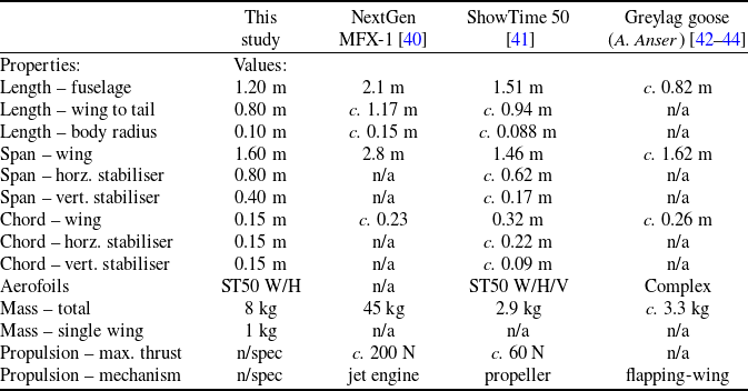

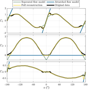

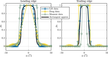


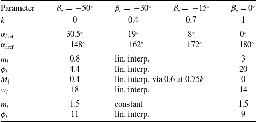

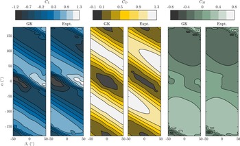


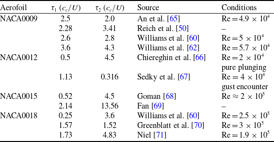
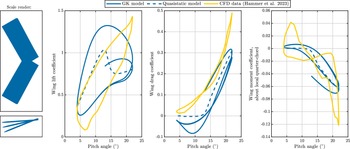
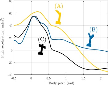


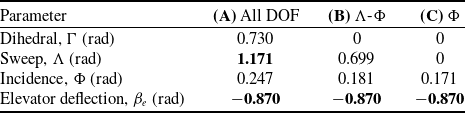
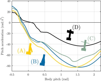


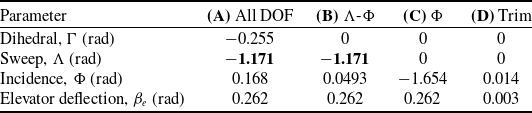


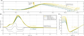


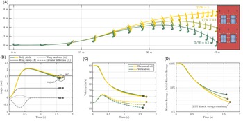


 Open access