


1. Introduction
Antarctic sea ice is a crucial factor in the climate and local marine ecosystems (Massom and Stammerjohn, Reference Massom and Stammerjohn2010). Since the 1970s, Antarctic sea ice extent underwent a period of slow increase until 2015 followed by a rapid decrease (Comiso and others, Reference Comiso, Parkinson, Gersten and Stock2008; Liu and Curry, Reference Liu and Curry2010). The extent broke its minimum low record in the Austral summers of 2017, 2022 and 2023 with an area of 2.11, 1.92 and 1.79 million km2, respectively (Gilbert and Holmes, Reference Gilbert and Holmes2024). Antarctic land-fast sea ice (LFSI) is attached to the shore, grounded icebergs and ice shelves. It has a longer lifetime than drift ice, and it can extend offshore up to hundreds of kilometres (Massom and others, Reference Massom, Hill, Lytle, Worby, Paget, Allison, Jeffries and Eicken2001b; Fraser, Reference Fraser2021, Reference Fraser2023). LFSI is first-year ice (FYI), apart from Fjords where second-year sea ice (SYI) has been found (Massom and others, Reference Massom, Hill, Lytle, Worby, Paget, Allison, Jeffries and Eicken2001b).
Investigations of land-fast ice, particularly in Prydz Bay, East Antarctica have been carried out extensively in the past. Under the Antarctic Fast Ice Network (AFIN) initiative (Heil and others, Reference Heil, Gerland and Granskog2011), the year-round logistic support provided by the Chinese Zhongshan station and other stations in the vicinity of Prydz Bay made sustainable snow and sea ice field experiments possible. The studies have focused on the impact of atmosphere conditions and seasonal oceanic heat flux on land-fast ice evolution (Heil and others, Reference Heil, Allison and Lytle1996; Heil, Reference Heil2006; Lei and others, Reference Lei, Li, Cheng, Zhang and Heil2010), local sea ice physical properties (Tang and others, Reference Tang, Qin, Ren and Kang2006; Yang and others, Reference Yang2016a) and seasonal and interannual land-fast ice mass balance (Li and others, Reference Li, Lei, Heil, Cheng, Ding, Tian and Li2023). Modelling studies have been carried out to understand the role of oceanic heat flux and albedo in the ice mass balance (Yang and others, Reference Yang, Zhijun, Leppäranta, Cheng, Shi and Lei2016b; Zhao and others, Reference Zhao, Yang, Shu, Shen, Tian, Hao and Zhao2021), the patterns of FYI and SYI during austral late autumn and early winter (Zhao and others, Reference Zhao, Cheng, Yang, Vihma and Zhang2017), the role of snow on land-fast ice evolution (Zhao and others, Reference Zhao2019a), sensitivity of parameterization in sea ice models (Liu and others, Reference Liu2022) and the internal structure of land-fast ice (Zhao and others, Reference Zhao2022b).
Snow cover on sea ice reveals large spatial variability (Massom and others, Reference Massom2001a; Webster and others, Reference Webster2018). In the Weddell Sea, the average annual snow depth is 0.5 m, with maximums up to 1.0 m (Eicken and others, Reference Eicken, Lange and Wadhams1994). Snow continues to accumulate throughout the year, with an average net accumulation of approximately 0.34 m (Arndt and Paul, Reference Arndt and Paul2018; Nicolaus and others, Reference Nicolaus2021). In contrast, in the Prydz Bay in the Indian Ocean sector, the average annual snow depth is only 0.2 m (Lei and others, Reference Lei, Li, Cheng, Zhang and Heil2010). Snow is a good insulator and limits ice growth but also protects the ice from melting (Maykut and Untersteiner, Reference Maykut and Untersteiner1971; Maykut, Reference Maykut and Untersteiner1986; Fichefet and others, Reference Fichefet, Tartinville and Goosse2000). On the other hand, snow may contribute to ice thickness by transforming into snow–ice and superimposed ice due to flooding, melt-freeze cycles and liquid precipitation (Shirasawa and others, Reference Shirasawa, Leppäranta, Saloranta, Kawamura, Polomoshnov and Surkov2005). For snow–ice formation, snow needs to be thick enough to push the ice surface below the sea level, causing flooding of seawater that forms slush for the source of snow–ice. Snow meltwater and rainwater act as the sources of superimposed ice. Frozen slush contributes to 5–25% of the total ice thickness in Antarctic seas (Jeffries and others, Reference Jeffries, Morris, Weeks and Worby1997; Haas and others, Reference Haas, Thomas and Bareiss2001; Massom and others, Reference Massom, Hill, Lytle, Worby, Paget, Allison, Jeffries and Eicken2001b).
In Prydz Bay, the LFSI is primarily seasonal and categorized as first-year ice (FYI). This means that the ice typically forms in March (austral early winter) and disintegrates by the end of December (austral early summer) (Lei and others, Reference Lei, Li, Cheng, Zhang and Heil2010). However, under certain conditions, a portion of the FYI LFSI may persist over summer and become SYI. The thermal regimes of FYI and SYI LFSI differ significantly. These differences can be identified through vertical ice temperature profiles, which influence ice growth rates, thermal inertia and cold content (the energy required to raise the ice temperature to the melting point).
We aim to answer the following questions: (1) How does precipitation impact the seasonal cycle of land-fast FYI and SYI?, (2) How does the initial ice condition impact the seasonal cycle of land-fast FYI and SYI? and (3) Can we find new knowledge to quantify snow and ice interaction on a local scale?
We used thermistor string data of snow and ice temperature, and borehole snow and ice thickness measurements over FYI and SYI LFSI from May to November 2019. Based on operational meteorological observations, ERA5 atmospheric reanalysis products, and a numerical sea ice model, snow and ice layer growth and interactions have been investigated. We go beyond Zhao and others (Reference Zhao, Cheng, Yang, Vihma and Zhang2017) investigation of the FYI and SYI transition process in March by investigating a longer period variation of FYI and SYI.
2. Data and method
2.1. Research site and climatological condition
The research site is in the coastal area of the Chinese Antarctic Zhongshan station (69°22ʹ24ʹʹS, 76°22ʹ40ʹʹ E) in the Prydz Bay (Fig. 1). The annual mean air temperature is − 9.9°C (Weigang and others, Reference Weigang, Wenqian, Maifeng, Jingkai and Xinfeng2022). The highest and lowest air temperatures recorded in history were 9.8°C and −45.7°C (Bian and others, Reference Bian, Ma, Lu and Lu2010; Yang and others, Reference Yang, Zhang and Li2010; Turner and others, Reference Turner, Marshall, Clem, Colwell, Phillips and Lu2020). Easterly and southeasterly winds prevail year-round in the region (Li and others, Reference Li, Lei, Heil, Cheng, Ding, Tian and Li2023), and wind speed shows clear annual variations with high values in Austral winter and low values in Austral summer. Wind affects the spatial distribution of snow in the Fjord along the direction of the prevailing wind (Yang and others, Reference Yang2016a; Zhao and others, Reference Zhao2019a). Precipitation at Zhongshan Station is predominantly solid, typically associated with cyclonic or storm events. Near the coastline, strong winds frequently drive the snow away from the ice, leaving the surface almost bare. In contrast, more than 1 km offshore, snow depth can reach 0.2–0.4 m (Yu and others, Reference Yu, Yang, Vihma, Jagovkina, Liu, Sun and Li2018; Zhao and others, Reference Zhao2019a). Affected by the prevailing wind from the continent, the local air is dry and the annual average humidity is 54%.
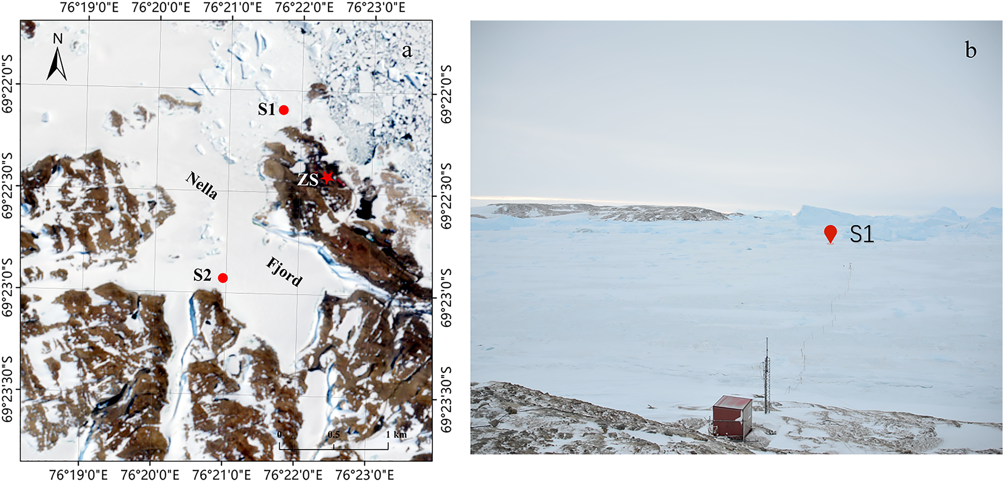
Figure 1. Research site. (a) Sentinel-2 satellite image (19 December 2019) of the Zhongshan station (red star), S1 (FYI) and S2 (multi-year ice: SYI) mark the observation sites of the thermistor-string based ice mass balance buoys and borehole snow depth and ice thickness. (b) Photograph taken in August 2019 looking toward Nella Fjord from the top of Tiane ridge, S2 is on the left outside of the photo frame.
The coastal area is predominantly covered by LFSI, extending 60–100 km in winter and 20–40 km in summer north of Zhongshan Station (Zhao and others, Reference Zhao2020). FYI grows from March to August, reaching a maximum thickness of about 1.7 m by October–November (Li and others, Reference Li, Lei, Heil, Cheng, Ding, Tian and Li2023). Ocean currents underneath LFSI are influenced by regional winds, sea ice distribution and inflow of ice-melt water (Hu and others, Reference Hu, Zhao, Heil, Qin, Ma, Hui and Cheng2023). The primary water masses in Prydz Bay and adjacent seas include Antarctic Surface Water, Prydz Bay Shelf Water, Circumpolar Deep Water and Antarctic Bottom Water. Temperature and salinity variations are most pronounced in the surface waters during summer months, while the warmer waters of the circumpolar deep layer remain relatively stable (Vaz and Lennon, Reference Vaz and Lennon1996; Yabuki and others, Reference Yabuki, Suga, Hanawa, Matsuoka, Kiwada and Watanabe2006).
2.2. In situ observations
As an active component of the AFIN program, snow and sea ice measurements off Zhongshan station are mandatory under the umbrella of the Chinese National Antarctic Research Expedition (CHINARE) voyages. The CHINARE 2019 expedition marked the 35th voyage. Two thermistor string-based ice mass balance buoys were deployed. They comprised temperature sensors, a data acquisition device and a power supply unit (Zuo and others, Reference Zuo, Dou and Lei2018). The temperature sensors were DS18B20, manufactured by DALLAS. The measurement range is between −55°C and 125°C with an accuracy of ± 0.5°C (Fezari and Al Dahoud, Reference Fezari and Al Dahoud2019). The length of the thermistor chains was 3 m and the sensor spacing was 3 cm. The data acquisition device included a clock module, a master control chip and an SD memory card. Once deployed, data are collected at a pre-set interval and stored in an SD card. The temperature chains were deployed in the boreholes so that the upper sensors were in the air, the chains extended through the snow and ice and the lowest sensors were in the water. The power supply unit delivers 3.3 V to the sensors and data acquisition device. Due to the low temperatures at the site, the power supply unit was equipped with a solar panel that charged the batteries when exposed to sufficient sunlight, ensuring stable long-term operation of the system.
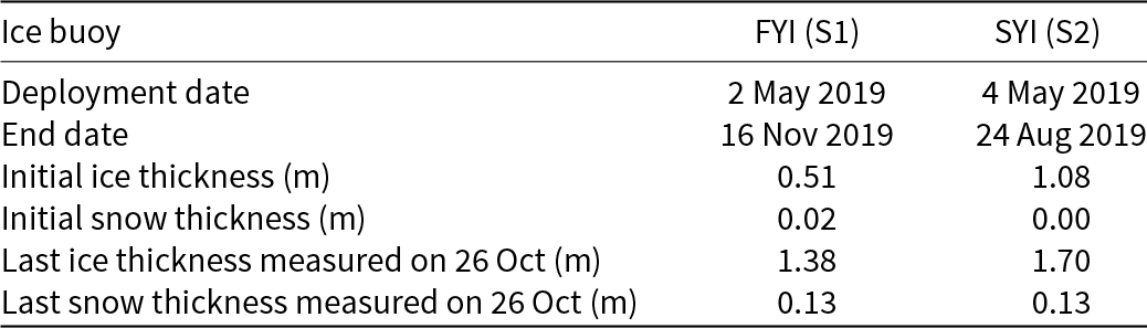
Two ice buoys were deployed on 2 and 4 May 2019 at the sites S1 (76.362°E, 69.368°S) and S2 (76.349°E, 69.382°S) (Table 1). S1 was located at the mouth of Nella Fjord, 1 km northwest of Zhongshan Station, usually covered by FYI between early March and late November. S2 was located inside Nella Fjord, where the ice is predominantly multi-year ice due to the terrain orientation (Zhao and others, Reference Zhao2020). The distance between the two sites was 1.6 km. The vertical temperature profiles were sampled every 2 h. Due to technical issues, the thermistor chain at S2 ended recording on August 24, while the thermistor chain at S1 worked continuously until November 16 when the buoy was recovered.
Table 1. Information on ice buoy deployment
Snow depth and ice thickness were measured manually by drilling boreholes using a 5 cm diameter auger. Three to five ice holes were drilled within a 10-m radius each time. Ice thickness was measured with an ice gauge from the boreholes, and snow depth was measured with a stainless-steel ruler at three sites located 1 to 5 m from each ice hole. In total, 30 and 29 sets of manual observations were collected at S1 and S2, respectively. The accuracy of the snow depth and ice thickness measurements is ± 0.5 cm.
The meteorological data were obtained from the Zhongshan automatic weather station (AWS): 10 m air temperature, 10 m wind speed and direction and relative humidity. Precipitation is not measured at Zhongshan Station but daily accumulated precipitation is available at the Russian Progress Station, 1 km east of Zhongshan Station.
2.3. ERA5 reanalysis data
The fifth generation of the European Centre for Medium-Range Weather Forecasts (ECMWF ERA5) reanalysis data provides global climate and weather information from 1940 to the present (Hersbach and others, Reference Hersbach2023). It utilizes ECMWF’s 4D-Var data assimilation and the Integrated Forecasting System (IFS), incorporating models and observations worldwide. Released in 2017, ERA5 replaced the ERA-Interim reanalysis data, offering higher spatial and temporal resolution. ERA5 is accessible as an online download service, updated daily with a delay of approximately 5 days (Hersbach and others, Reference Hersbach2023). We extracted 10 m wind speed, 10 m air temperature, relative humidity, incident shortwave radiation, atmospheric longwave radiation and precipitation. The original ERA5 products have a spatial resolution of 0.25° × 0.25° and a temporal resolution of 3 h. In this study, a bilinear spatial interpolation was used to increase the spatial resolution to 0.125° × 0.125°. The nearest point to Zhongshan station was picked up, and a temporal linear interpolation was applied to obtain a time series with a 1-h time step.
2.4. HIGHTSI model configuration
The one-dimensional high-resolution thermodynamic snow and ice model (HIGHTSI) was applied in the study (Launiainen and Cheng, Reference Launiainen and Cheng1998). HIGHTSI solves the heat conduction equation for the snow and ice layers separately. The upper boundary is the surface skin temperature coupled with the surface heat balance. The surface temperature is solved by Newton’s iteration method from the surface heat balance. The lower boundary of ice is fixed at the freezing temperature of seawater (−1.8°C) in this study, and the boundary moves due to melting and freezing as quantified by the upward oceanic heat flux and the conductive flux into the ice. Surface and sub-surface melting is calculated from the surface heat balance and solar heat absorption within snow and ice layers (Cheng and others, Reference Cheng, Vihma and Launiainen2003; Zhao and others, Reference Zhao2022b). Snow accumulation resulted from precipitation, and part of the snow layer may form slush with sea water, melt water, or rain and turn into snow–ice or superimposed ice (Leppäranta, Reference Leppäranta1983; Shirasawa and others, Reference Shirasawa, Leppäranta, Saloranta, Kawamura, Polomoshnov and Surkov2005). Snow-depth changes also due to snow metamorphosis. Ice growth slows down due to the insulation of snow (Wang and others, Reference Wang, Cheng, Wang, Gerland and Pavlova2015) or steps up due to the formation of snow–ice (the snow was heavy enough to overcome the buoyancy of ice, and was mixed with seawater to form slush that was subsequently refrozen) and superimposed ice (snow meltwater percolated deep down to the snow–ice interface and refroze) (Cheng and others, Reference Cheng, Vihma and Launiainen2003).
In the HIGHTSI model, the prognostic variables are temperature distribution and snow depth, slush, snow–ice, superimposed ice and congelation ice. The snow depth accumulation is converted from snowfall (given as snow water equivalent, SWE) with a fixed snow density, and snow melting is calculated by the surface heat balance. Slush, snow–ice and superimposed ice are modelled directly as described above, and congelation ice is formed or melted at ice bottom. We assume snow–ice and superimposed ice were formed at the snow–ice interface and these components are integrated with congelation ice to form the total ice thickness. For simplicity, we assumed superimposed ice formation occurred at the onset snow melt so that meltwater drains down to ice surface to act as the source. The density of accumulated snow is parameterized according to Anderson (Reference Anderson1976), and the density of slush is calculated as a function of density of snow, ice and water (Saloranta, Reference Saloranta2000). The basic equations and parameters of the model are summarized in a supplemental file (Table S1), with the applied values of the parameters provided in Table A1.
The essential atmospheric forcing data are wind speed ( ${V_a}$), air temperature ( ${T_a}$), relative humidity ( ${R_h}$), precipitation ( $Prec$) and downward shortwave ( ${Q_s}$) and longwave radiative ( ${Q_l}$) fluxes. In this study, ${V_a}$ ${T_a}$ and ${R_h}$ came from AWS observations, and $Prec$, ${Q_s}$ and ${Q_l}$ were ERA5. Preliminary modelling trials revealed that the ERA5 precipitation overestimated snow accumulation. ERA5 data interpolated to 0.125° resolution are not always well representative in a local study in a strongly heterogeneous terrain. The uncertainties of ERA5 precipitation over the Antarctic have been investigated by Roussel and others (Reference Roussel, Lemonnier, Genthon and Krinner2020) who found that the ERA5 precipitation errors in areas of complex topography can be up to 50 %. Therefore, we applied 50% reduced precipitation (0.39 mm day−1) as the model input (Yu and others, Reference Yu, Yang, Vihma, Jagovkina, Liu, Sun and Li2018). This setup has been justified for multidecadal simulations of Canadian Arctic land-fast ice where snow drift was strong (Wang and others, Reference Wang, Zhao, Cheng, Hui, Su and Cheng2024).
In situ observations have indicated that the oceanic heat flux  ${F_w}$ has an annual cycle in Prydz Bay (Heil and others, Reference Heil, Allison and Lytle1996; Lei and others, Reference Lei, Li, Cheng, Zhang and Heil2010; Yang and others, Reference Yang, Zhijun, Leppäranta, Cheng, Shi and Lei2016b). The highest values appear during the late Austral summer and early autumn, i.e. after summer ice breakup and beginning of new ice season. When ice is formed in March, ${F_w}$ decreases drastically and remains small until November when ice starts to melt and sunlight warms the water beneath sea ice. For model simulation during the cold season, we used the fixed value of 6 W m−2 (Zhao and others, Reference Zhao, Cheng, Yang, Vihma and Zhang2017).
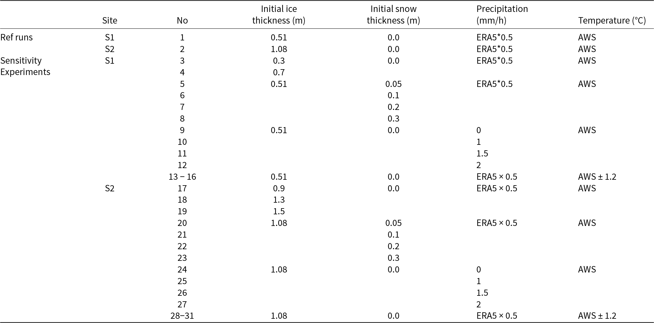
To fulfill the objectives, we designed modelling experiments as follows: (a) Two reference runs, Ref (S1) and Ref (S2), applying the observed initial condition of S1 and S2. The meteorological and oceanic boundary conditions were the same. (b) Sensitivity experiments for snow depth and initial ice thickness (Table 2). Sensitivity experiments on snow, snow–ice and superimposed ice formation have been done before (Zhao and others, Reference Zhao2019a), and here we went further by using more realistic model conditions. The impacts of initial snow and ice thickness, temperature and snowfall on snow and ice mass balance were also investigated. The initial temperature was linearly interpolated between air temperature and freezing temperature at ice bottom. The model simulations started on 4 May and lasted until 30 November.
Table 2. Summary of the modelling experiments
2.5. Analytical ice growth model
During cold conditions, ice growth can be estimated using an analytical quasi-steady model (Leppäranta, Reference Leppäranta1993), known as the Zubov’s law:
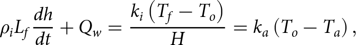 \begin{equation}{\rho _i}{L_f}\frac{{dh}}{{dt}} + {Q_w} = \frac{{{k_i}\left( {{T_f} - {T_o}} \right)}}{H} = {k_a}\left( {{T_o} - {T_a}} \right),\end{equation}
 where  ${\rho _i}$ is the sea ice density at the basal layer, ${L_f}$ is the latent heat of freezing, $h$ is the ice thickness, $t$ is time, ${k_i}$ is the thermal conductivity of sea ice, ${T_f}$ is the sea water freezing point, ${T_o}$ is the ice surface temperature, ${T_a}$ is air temperature, ${k_a}$ is air-ice exchange coefficient and ${Q_w}$ is the oceanic heat flux. Given the initial condition $h\left( 0 \right) = {h_0}$ and ${Q_w} = 0$, we have:
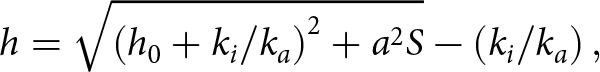 \begin{equation}h = \sqrt {{{\left( {{h_0} + {k_i}/{k_a}} \right)}^2} + {a^2}S} - \left( {{k_i}/{k_a}} \right),\end{equation}
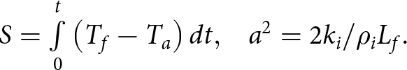 \begin{equation}S = \mathop {\smallint} \limits_0^t \left( {{T_f} - {T_a}} \right)dt,\,\,\,\,\,{a^2} = 2{k_i}/{\rho _i}{L_f}.\end{equation}
 Here  $S$ is the freezing-degree-days (FDD) in °C day, ${{{\rho }}_i}$, ${{\text{L}}_f}$, and ${{\text{k}}_{\text{i}}}$ were set to 910 kg m−3, 333.4 kJ kg−1 and 2.2 W m−1 °C−1, respectively, and ${{\text{k}}_{\text{i}}}/{{\text{k}}_{\text{a}}}$ was set to 10 cm.
3. Results and discussion
3.1. Meteorological conditions
The scatter plot comparison of  ${V_a}$, ${T_a}$ and ${R_h}$ between AWS and ERA5 is given in Figure 2. For wind speed, the agreement was reasonable (R 2 = 0.50). The mean AWS and ERA5 values were 5.2 m s−1 and 5.3 m s−1, respectively. The time series of AWS wind speed (Figure A1) indicated five peaks larger than 15 m s−1 between May and November, and ERA5 reproduced such high events. For weak winds (< 5 m s−1), ERA5 tended to overestimate the values, while the opposite was true for high winds. The easterly wind direction dominated in the study period (Figure 3) in line with the climatological wind conditions (Zhao and others, Reference Zhao2019b; Li and others, Reference Li, Lei, Heil, Cheng, Ding, Tian and Li2023).
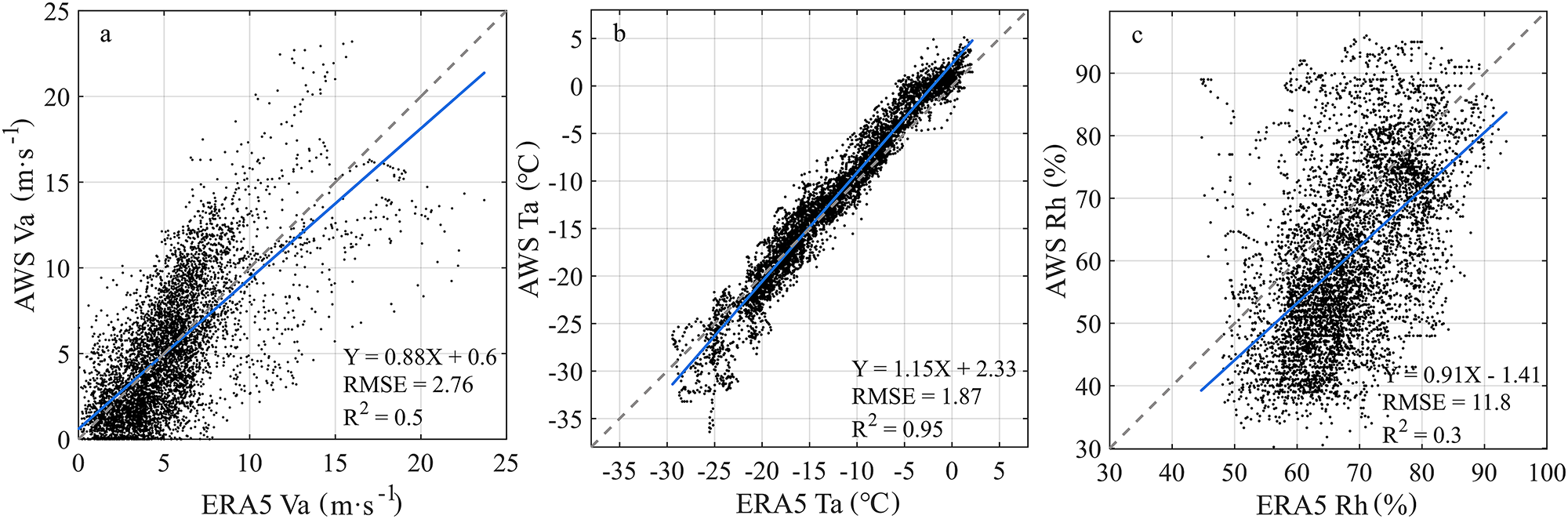
Figure 2. The scatter plot of AWS and ERA5 data during the investigation period; wind speed (a), air temperature (b) and relative humidity (c).
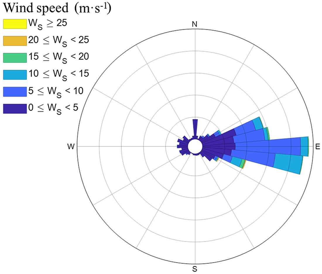
Figure 3. Wind rose diagram based on the data collected from AWS from 1 May 2019, to 31 Dec 2019. The colours represent different wind speed intervals.
The correlation between AWS and ERA5 air temperature was high (0.97), but ERA5 tended to overestimate/underestimate low/high temperatures. During the study period, for  ${T_a}$ < − 20°C ERA5 showed a warm bias of 2.1°C, while for ${T_a}$ > − 5°C, ERA5 had a cold bias of 2°C. Overall, ERA5 had a cold bias of 0.54°C with a root mean square error (RMSE) of 2.3°C. In the melting period between November and January, ERA5 air temperature revealed 2.1°C cold bias. The observed and ERA5-modeled humidity values were scattered. On average, the ERA5 relative humidity was 7.53 ± 0.15% lower than the AWS recordings.
3.2. Snow and sea ice observations
Snow depth and ice thickness observed at S1 and S2 both showed similar, distinguished features (Figure 4a). Over the entire observation period, the mean snow depths were 0.12 m and 0.14 m at S1 and S2, respectively, and the difference is attributed to surface topography and wind conditions. During the survey period, there were three peaks in snow depth where increase was associated with heavy snowfall while decrease was due to snow drift by strong wind (Figure 4b).
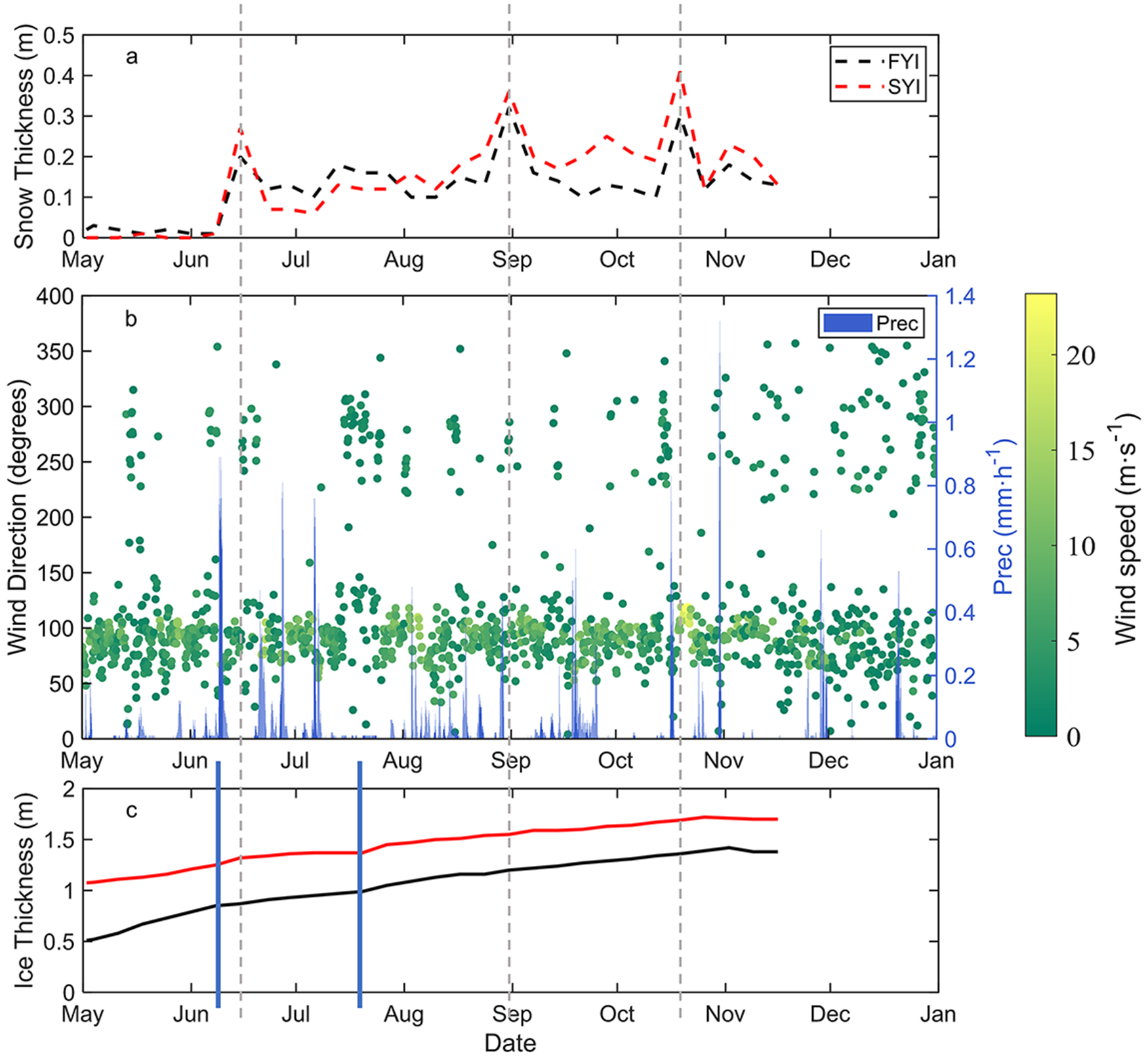
Figure 4. (a) Snow depth at S1 and S2, (b) wind speed and direction by AWS, hourly precipitation from ERA5 and (c) ice thickness at S1 and S2. The vertical grey dashed lines mark the snow episodes (maximum snow accumulation), and the blue bars mark the moments when snow started to accumulate (left) and ice growth rate changed (right).
Initial ice thicknesses at S1 and S2 differed from each other (Figure 4c), which resulted in different ice growth rates. Before snow accumulation, ice grew at S1 by 9.2 mm/day, nearly twice as fast as at S2 (4.7 mm day−1). When the first major snow accumulation event began on 10 June, the ice growth rate for FYI slowed to 3 mm day−1, while the SYI site showed an increase in the ice growth rate to 10 mm day−1 until the snow depth reached its maximum peak on 15 June. The decrease in the ice growth rate at S1 was due to the immediate snow insulation effect. The observed increase in the ice growth rate (calculated from two successive in situ visits) at S2 in response to snow accumulation can only be explained by snow–ice formation. During this period, the ice thickness was 1.28 m, assuming snow and ice densities of 300 kg m−3 and 900 kg m−3, respectively. A snow-flooding event (required to form slush for snow–ice formation) would necessitate a minimum snow depth of about 0.44 m. However, the maximum observed snow depth was only 0.26 m on 15 June, it was too thin to facilitate snow–ice formation. Thus, this apparent ice thickness increase is likely attributable to measurement bias or heterogeneity in the SYI bottom (Zhao and others, Reference Zhao, Cheng, Vihma, Lu, Han and Shu2022a). From 15 June onward, the ice growth rates were 3.4 mm day−1 (close to the ice growth rate between 10 and 15 June) for FYI and 2.9 mm day−1 for SYI, respectively, until 20 July, when both stabilized at an almost constant rate of 3.5 mm day−1. Thus, FYI responded stronger to initial snow accumulation than SYI. The ice temperature buoys worked well during this period (cf. Fig. 7). The temperature gradient represented the ice growth in good agreement with the borehole observations. The details are given in the following section.
3.3. Snow and ice modelling
3.3.1. Control runs
The modelled snow depth at S1 and S2 were almost the same since we applied the same ERA5 precipitation (50%) as the external forcing (Fig. 5). The simulated snow depth could not reproduce large snowfall events on June 15, August 31 and October 19 because the HIGHTSI model does not include snow drift which was evident in the observations. The modelled onset of snow melting agreed with observations indicating a good simulation of the surface energy balance. The modelled snow depth was in agreement with observations at S2 since the site was inside the narrow fjord surrounded by hills (Fig. 1a) where snow drift was limited. The modelled mean and maximum snow depths were 0.11 m and 0.24 m at both sites, and the corresponding observed mean and maximum values were 0.12 m and 0.32 m for S1 and 0.14 m and 0.41 m for S2, respectively. The modelled mean and maximum snow depths were 92% and 75% of the observed values at S1, and 79% and 59% of the observed values at S2.
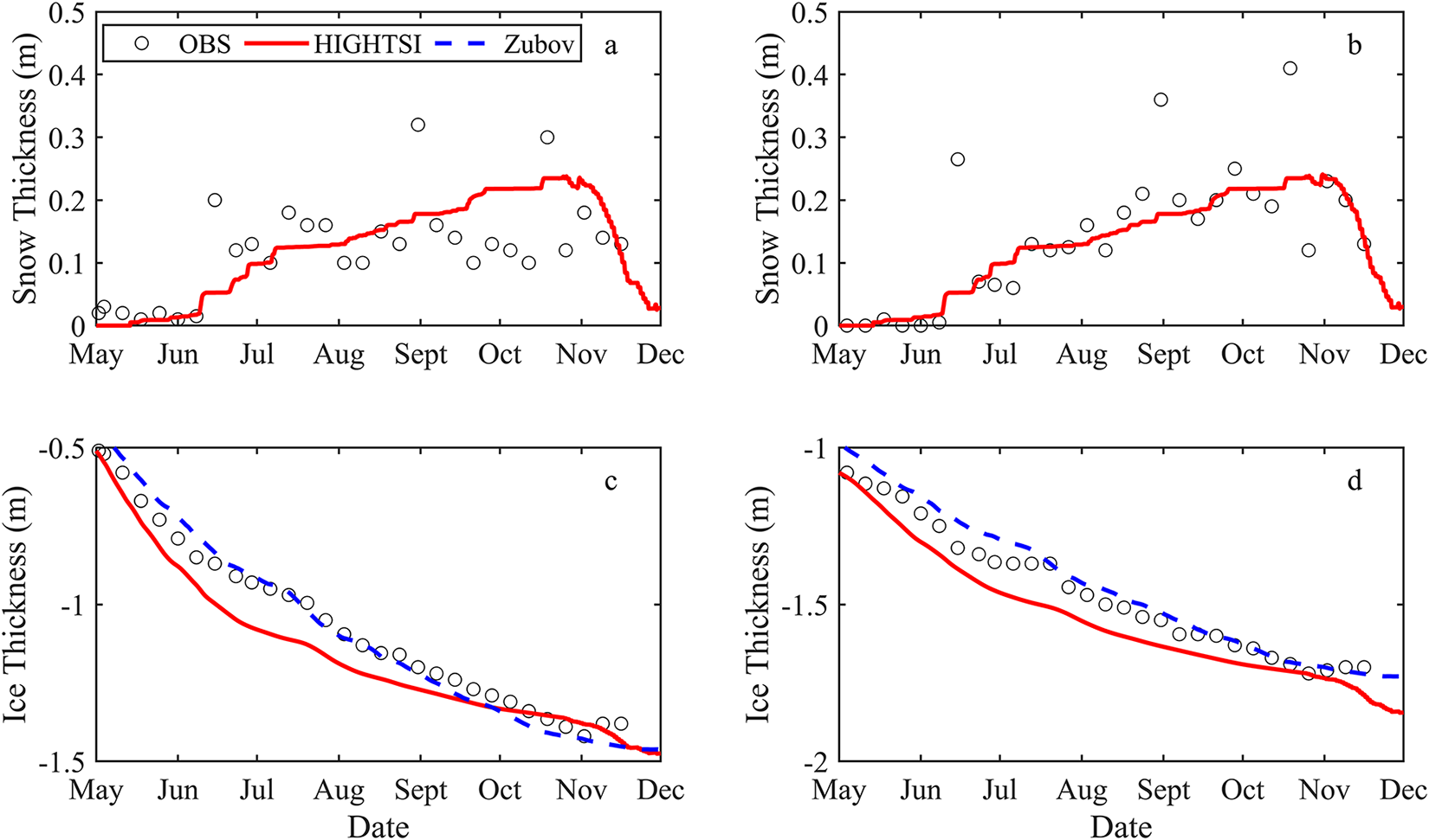
Figure 5. Time series of snow depth and ice thickness at S1 (a, c) and S2 (b, d) sites. The solid lines are for HIGHTSI model (red) and Zubov analytical model (blue), and the circles are observed values.
The agreement between the observations and model is better for ice thickness at both sites than for snow depth. By the end of the simulation, ice thickness at S1 and S2 reached 1.47 and 1.84 m, respectively, when the modelled FYI and SYI thickness had increased by 0.96 and 0.76 m, respectively. The bias (positive in both cases) and RMSE of the model results were, respectively, 0.08 m, 0.09 m for S1 and 0.07 m, 0.08 m for S2. The overestimation of ice thickness between late May and early October for both model runs may be attributed to the model’s failure to catch up with the heavy snowfall events in June, August and October. The analytical model (blue lines in Fig. 5) indicated a better fit of the ice thickness: the bias and RMSE were 0.04 m, 0.05 m for S1 and 0.03 m, 0.04 m for S2, respectively.
3.3.2. Growth rate
The modelled ice growth rate reproduced the periods (defined by blue bars in Fig. 4c) of the observed ice growth characteristic nicely (Fig. 6). Before snow accumulation, the growth rate was higher in FYI (11.2 mm day−1) than in SYI (6.9 mm day−1). Once the snow accumulation started, growth slowed. First, FYI grew slightly faster (4.4 mm day−1) than SYI (3.9 mm day−1), and from 19 July their growth rates were the same (1.9 mm day−1). The mean and maximum values were 0.44 cm day−1 and 1.0 cm day−1 for observations and 0.46/0.43 cm day−1 and 1.57/1.08 cm day−1 for HIGHTSI/Zubov model at S1. The corresponding values at S2 were 0.32 cm day−1 and 0.6 cm day−1 for observations, and 0.36/0.31 cm day−1 and 0.86/0.65 cm day−1 for HIGHTSI/Zubov model.
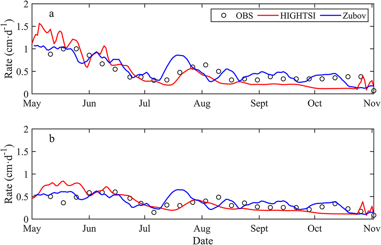
Figure 6. The observed and modelled sea ice growth rate at (a) S1 and (b) S2 sites. The hourly ice growth rate was smoothed by a 5-day moving average.
3.3.3. Surface temperature
The HIGHTSI model captures well the surface temperature evolution (Fig. 7). It tends to overestimate the cold peaks. The discrepancy between the observed and modelled surface temperature is related to the accuracy of snow depth.
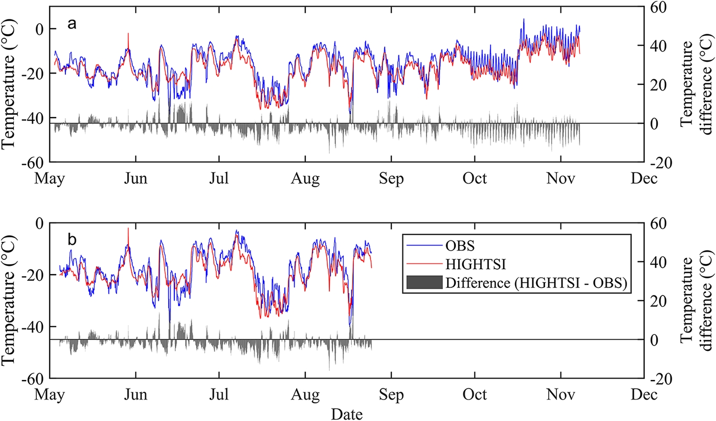
Figure 7. Observed and modeled surface temperature and the differences (mod−obs) for S1(a) and S2 (b) sites. The observed surface temperature was extracted by linear interpolation based on snow depth (or ice thickness), and readings from the thermistor sensors of ice-tethered buoys closest to the surface).
3.3.4. Ice temperature
The modelled temperature showed comparable patterns with the observations (Fig. 8). Based on observed snow condition and vertical ice temperature patterns, the modelling period was divided into five stages: Snow-free stage I, Rapid snow accumulation stage II, Cold period III, Warm-up period IV and Snow melting period V. Two types of correlation coefficients were calculated. The correlation coefficient between temperature profile (Corr (p)) refers to the correlation between modelled and observed average vertical temperature profile for a given period. The temporal correlation coefficient (Corr (t)) refers to the correlation between modelled and observed vertically averaged ice temperature over the entire ice layer. The adjustment time scale of the temperature profile is  ${h^2}\rho c/k\ 10$ day in the diffusion process.
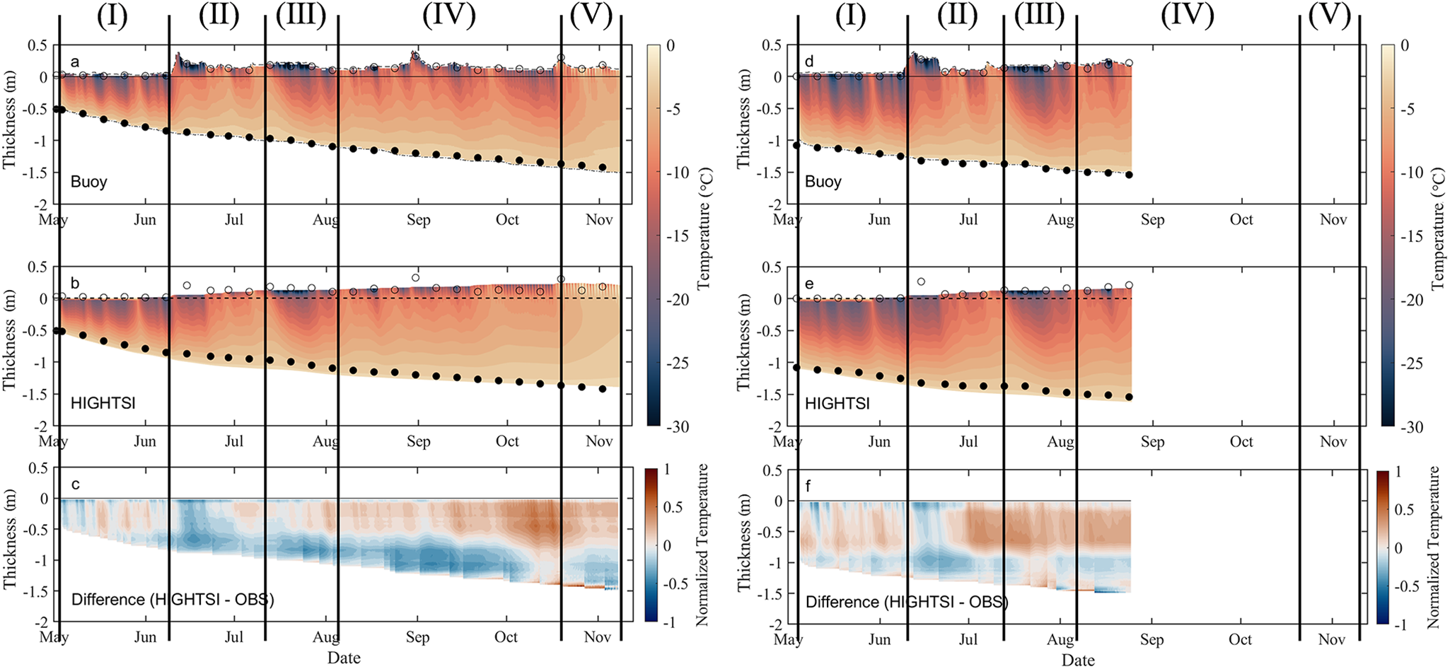
Figure 8. Observed and modelled ice temperature and their difference at site S1 (a, b, c) and S2 (d, e, f). The circles and black dots are manually observed snow depths and ice thickness, respectively. Note different time windows for S1 and S2.
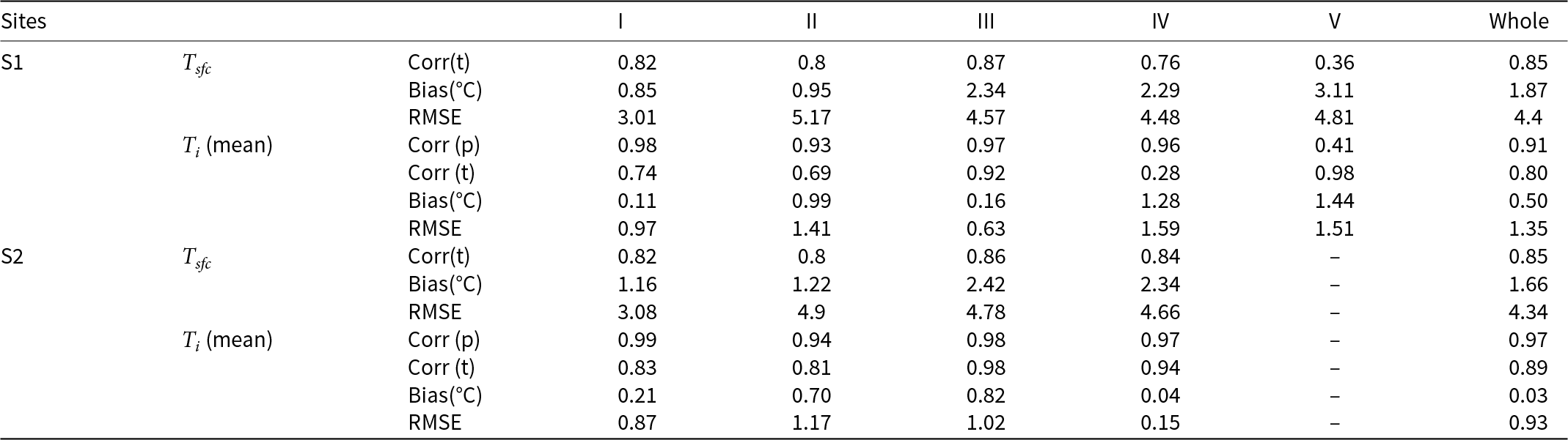
The results of the HIGHTSI model fit are shown in Table 3. The outcome was good in free conditions (Stage I) while snow accumulation in Stage II introduced strong insulation effect damping of the upward conductive heat flux. Because of the poor snow-depth simulation, the agreement between observed and modelled ice temperature was reduced. Stage III was dominated by a strong cold outbreak, when air temperature dropped below −30°C with the mean value of −22°C (Figure A1), and snow depth remained stable. The simulated ice temperature was improved. In Stage IV, the error of modelled ice temperature was larger at S1 than at S2 because the modelled snow depth was essentially identical for both sites, whereas the observed snow depths were different. In Stage V, the ice temperature increased and the ice growth period ended. For both sites, the correlation coefficients between temperature profiles were higher than the temporal correlation coefficients.
Table 3. Statistics of modelled temperature fit in five stages;  ${T_{sfc}}$ and ${T_i}$ represent the surface temperature and mean ice temperature, respectively
The ice temperature data allows us to estimate the first-order cold content ( $CC$) of ice, i.e. the amount of energy required to raise the temperature of ice to the melting point (Parajuli and others, Reference Parajuli, Nadeau, Anctil and Alves2021). $CC$ is defined as:
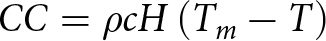 \begin{equation}CC = \rho cH\left( {{T_m} - T} \right)\end{equation}
 where  $\rho $ is the density, $c$ is the specific heat, $H$ is the thickness, $T$ is the mean temperature and ${T_m}$ is the melting temperature. The sea ice density is assumed constant (910 kg m−3), and the specific heat of sea ice is a function of ice temperature and salinity (Ono, Reference Ono1967). In Prydz Bay, the average ice salinity is 4 psu (Lei and others, Reference Lei, Li, Cheng, Zhang and Heil2010).
Applying average ice temperature, the modelled and observed cold content are estimated (Fig. 9). The correlation coefficient between the observed and modelled average normalized ice temperature was 0.91 for S1 and 0.97 for S2. The large discrepancy in ice temperature was associated with snow depth in mid-June and early October. The underestimation of snow thickness in the simulations resulted in increased temperature in the upper ice layer. In the period 2 May–24 August, the mean CC for S1 and S2 were 21.01 MJ m−2 and 32.78 MJ m−2, respectively.
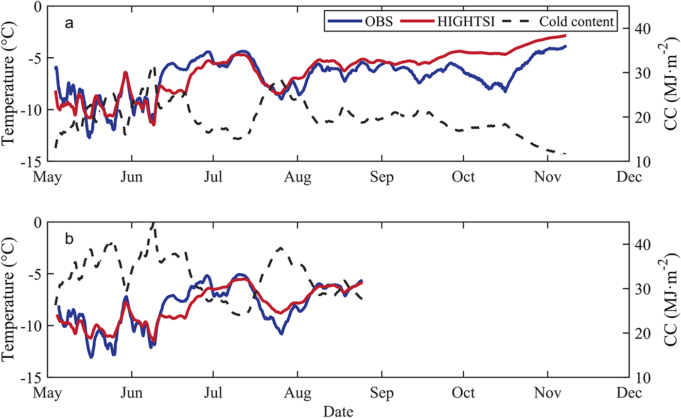
Figure 9. Observed and modelled average ice temperature and estimated cold content during the simulation period when ice-tethered buoys observations are available for s1(a) and s2(b). see figure legend for calculated components.
The ice temperature profiles were compared at six selected time instants (Fig. 10). The model could reproduce a vertical temperature gradient with the mean values of 9.4°C m−1 and 9.6°C m−1 for S1 and S2, respectively, while the corresponding observed values were 7.7°C m−1 and 5.2°C m−1. During the simulation period, a linear temperature profile dominated. As long as sunlight was weak, nonlinearities were caused by thermal inertia. In Figure 10, ice was gaining heat in profiles a, b, e, f, losing heat in profile d, while profile c was linear, in steady state. The biased modelled temperatures in b and f were caused by the biased snow depth (c.f. Fig. 8). In late October, the increasing solar radiation (Zhao and others, Reference Zhao, Cheng, Vihma, Lu, Han and Shu2022a) added on the nonlinearity of ice temperature profiles in both observed and modelled cases.
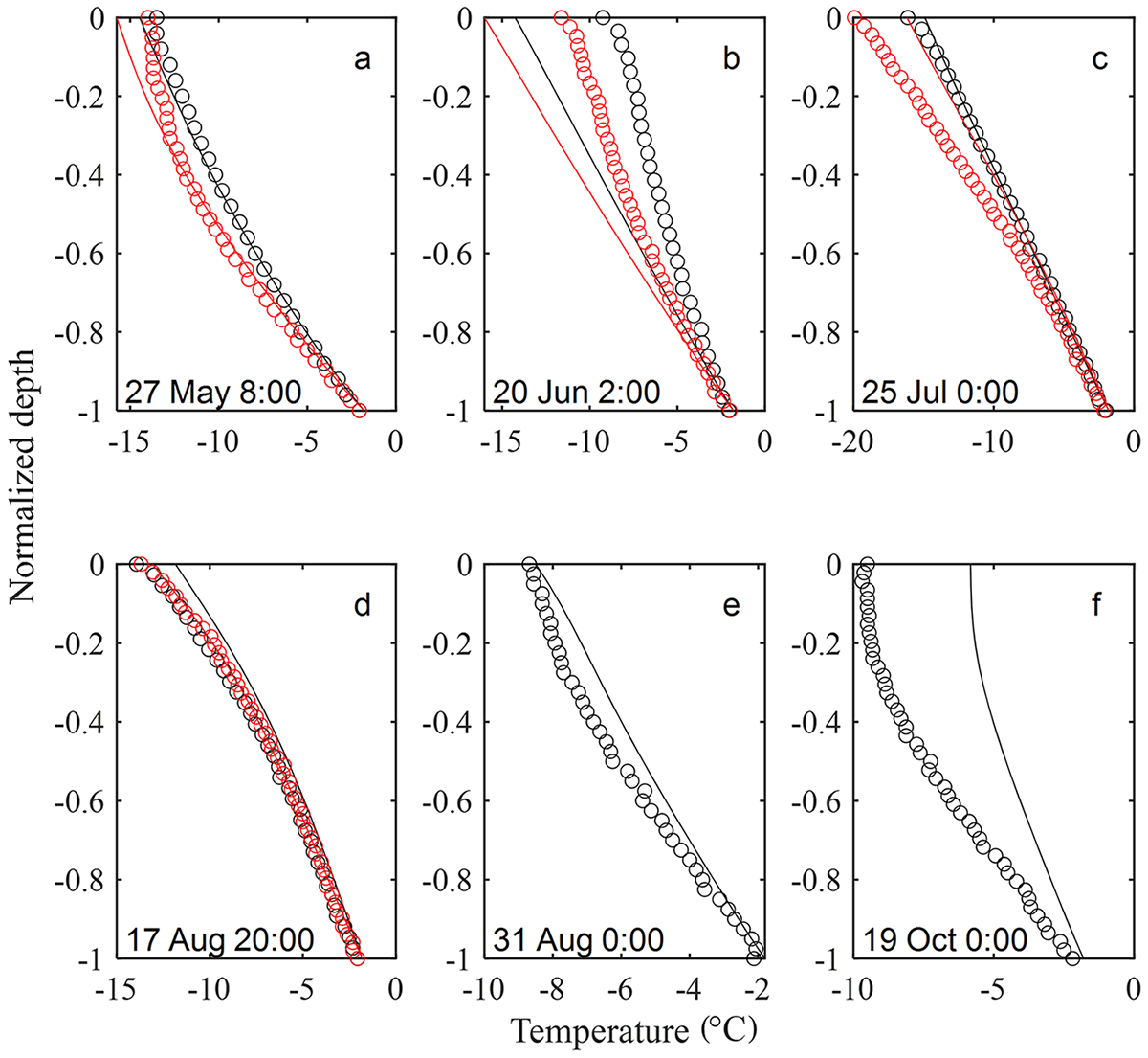
Figure 10. Selected ice temperature profiles. The solid lines are model results for S1 (red) and S2 (black), and the circles are observations for S1 (red) and S2 (black). the profiles are normalized to [−1,0] where 0 is ice surface and −1 is ice bottom.
3.4. Sensitivity modelling experiments
The sensitivity study examines how the modelled snow and ice layers react to initial and weather conditions. The sensitivity can be in general studied using the differential method which gives the sensitivity of  $F\left( {{p_1}, \ldots ,{p_m}} \right)$ to ${p_i}$ as $\delta F = \left( {\partial F/\partial {p_i}} \right)\delta {p_i}$ (e.g., Fichefet and Maqueda (Reference Fichefet and Maqueda1997); Yang and others, (Reference Yang2016a); Leppäranta (Reference Leppäranta2023)). Here, we considered the maximum-modelled snow depth, ice thickness, snow–ice and superimposed ice, as well as the net ice thickness budget.
For analytical model, according to the Eq. (2), ignoring the constant  ${k_i}/{k_a}$, the maximum ice thickness is ${h_{max}} = \sqrt {{h_0}^2 + {a^2}{S_{max}}} $ and the sensitivity is
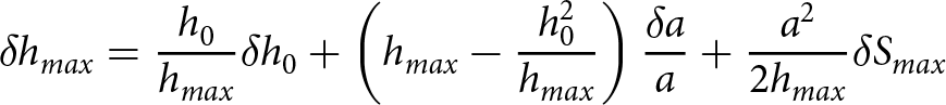 \begin{equation}\delta {h_{max}} = \frac{{{h_0}}}{{{h_{max}}}}\delta {h_0} + \left( {{h_{max}} - \frac{{h_0^2}}{{{h_{max}}}}} \right)\frac{{\delta a}}{a} + \frac{{{a^2}}}{{2{h_{max}}}}\delta {S_{max}}\end{equation}
 The sensitivity to  ${h_0}$ is small for small ${h_0}$ and approaches $\delta {h_0}$ for ${h_0} \to {h_{max}}.$ The sensitivity to $a$ is proportional to ${h_{max}}$ when ${h_0} \to 0$; for example, if a climatic mean of $a$ is used, then $\delta a/a \approx 0.2$, and $\delta {h_{max}} \approx 0.2 \cdot {h_{max}}$ (Fig. 11).
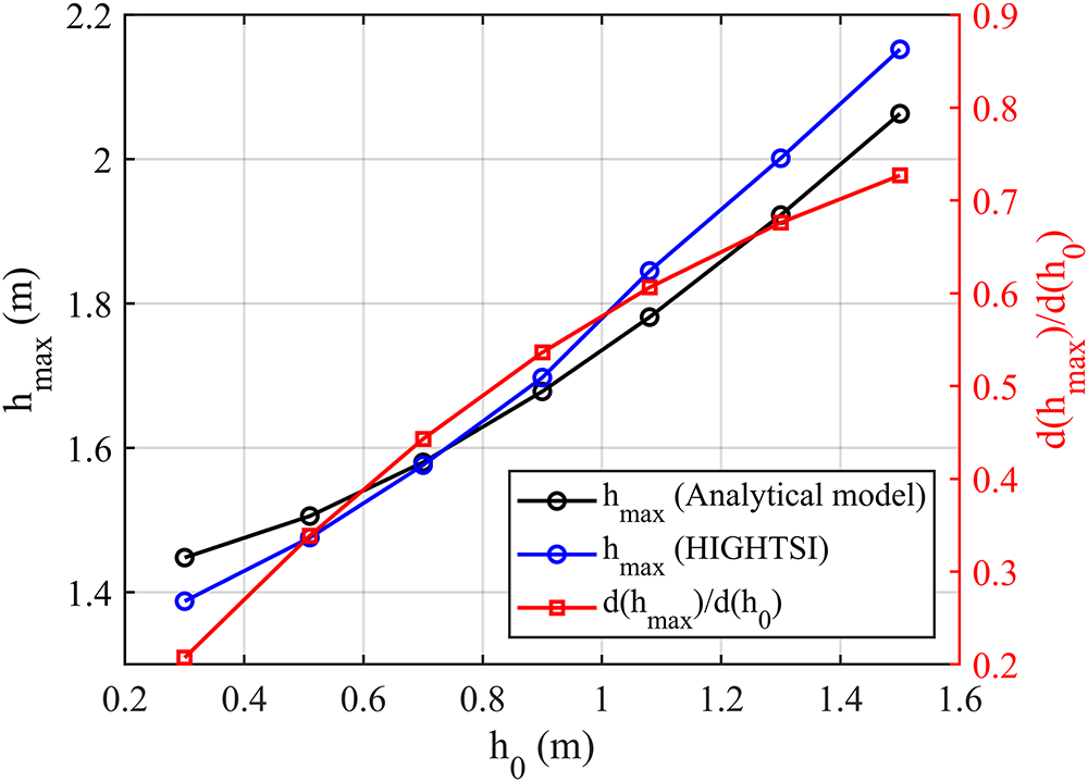
Figure 11. Model maximum ice thickness vs. initial ice thickness by Zubov and HIGHTSI models in the simulation period, and the sensitivity of the Zubov model to the initial ice thickness (red line).
The sensitivity of the HIGHTSI maximum ice thickness is proportional to the initial ice thickness (Fig. 12a), similar with the scaling analyses by Zubov model (Eq. 5). In this case, the initial ice thickness does not affect the modelled snow depth because there was no slush formation, and the modelled average snow depth remained unchanged as well as for the source-superimposed ice in melt–freeze cycles. The maximum FYI and SYI thicknesses are inversely related to the initial snow depth (Fig. 12b) due to the strong insulation effect of snow. The initial snow depth was too small to trigger snow–ice formation. The modelled maximum thickness of superimposed ice was proportional to the increase of initial snow depth because thicker snow generates more surface melting.
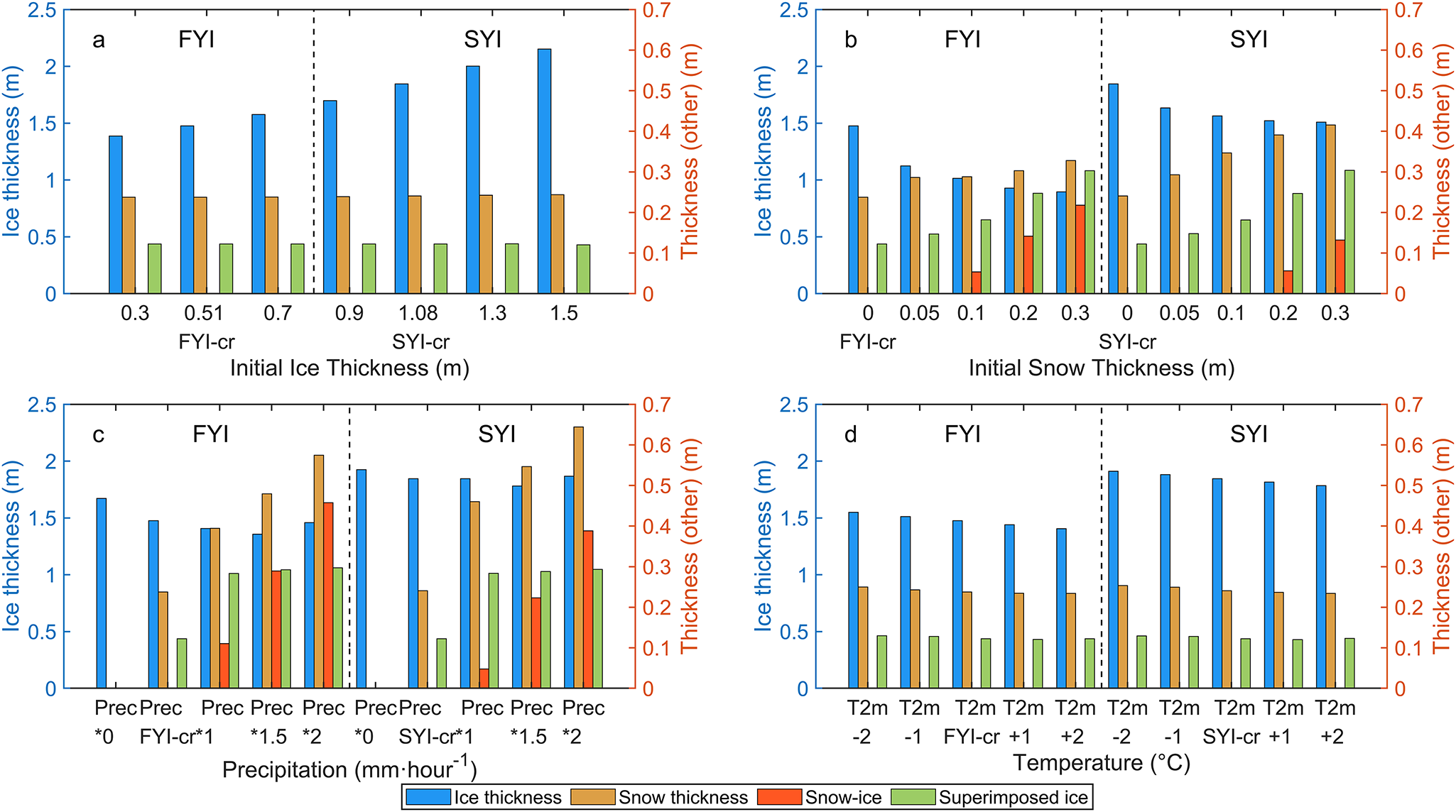
Figure 12. Modelled maximum snow depth and ice thickness in sensitivity experiments (Table 2) in response to (a) the initial ice thickness; (b) initial snow depth; (c) total precipitation and (d) air temperature. The simulations were made from 1 May to 31 Dec 2019. The ice thickness is presented on the left y-axis, while all other values (snow depth, snow-ice and accumulated superimposed ice) are shown on the right y-axis.
Increasing precipitation created more insulation that reduced the maximum ice thickness (Fig. 12c). With enough precipitation, snow–ice formation process was triggered. Snow–ice and also superimposed ice formation could overcome the snow insulation effect, and as a result, the maximum ice thickness started to slightly increase. Air temperature change has a negative linear effect on the maximum ice thickness (Eq. 5, Fig. 12d). Also, a higher air temperature brought a thinner snow cover and superimposed ice layer and vice versa.
Figure 13 illustrates the sensitivity of ice thickness to initial conditions and forcing (see Table 2 for more information of the model experiments). We focus on ice growth season between 2 May and 28 October. Ice growth was inversely related to the initial ice thickness (Fig. 13a); in the Zubov solution, the sensitivity is  $\delta \left( {D{H_i}} \right) = - \left( {D{H_i}/{H_{max}}} \right)\delta {h_0}$. Ice growth has an inverse relation to increasing initial snow depth (Fig. 13b). Also, due to the inverse relationship between conductive flux and snow depth, one would expect to see much more significant differences in ice growth for the exact change in snow depth when snow is thin, i.e. ice thickness growth is more sensitive to the thin snow. The more initial snow depth, the more snow–ice formation occurs. The impact of less precipitation is dominated by the insulation effect, while more precipitation increases the ice growth due to snow–ice formation (Fig. 13c). An increase of air temperature generates higher FYI growth than SYI growth (Fig. 13d).
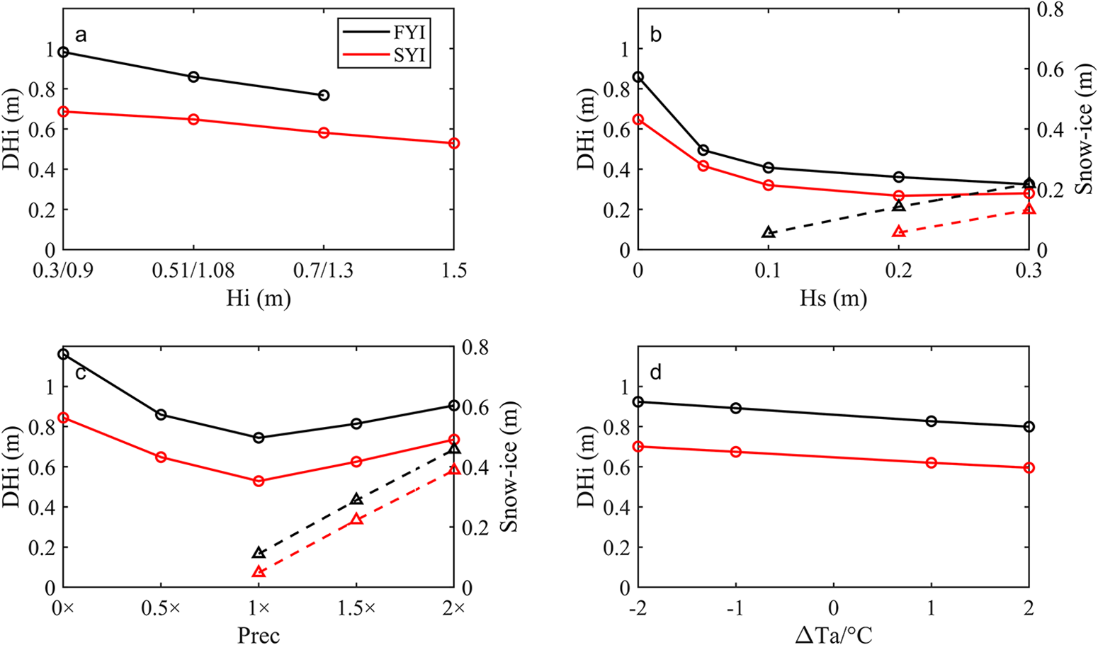
Figure 13. The sensitivity of ice growth during the freezing period (2 May–28 Oct) to (a) initial ice thickness; (b) initial snow depth; (c) precipitation and (d) air temperature. In panels (b) and (c), dashed lines (right-axis scale) show the sensitivity of snow–ice formation to initial snow depth and precipitation. The pair numbers in (a) x-axis represent the initial ice thickness for FYI and SYI, respectively.
3.5. Discussion
To our knowledge, this is the first time two thermistor-string-based ice mass balance buoys have worked simultaneously in FYI and SYI sites in Prydz Bay for such a long period. The buoys were deployed close to the coast for easy maintenance. Ideally, the buoys should have been deployed further offshore as the weather conditions change drastically along the fetch from the in-land ice sheet toward the marginal sea ice zone. The variability of air temperature near the coast is much weaker than over the inland ice sheet (Ding, Reference Ding2022). Measurements offshore would be more representative of the marine weather conditions, particularly for snow depth. We recommend ice mass balance buoys be deployed 10 km from the coast in the future to better monitor snow and ice interaction processes.
We have demonstrated the good performance of the snow and ice thermodynamic model HIGHTSI. The CICE-based single column Icepack (Version 1.1.0) can simulate equally well Prydz Bay sea ice thermodynamic mass balance using ERA5 reanalysis products (Hao and others, Reference Hao, Wang and Sun2024). Snow accumulation, however, was liable for errors in both studies. Excessive precipitation led to overestimated snow depth (Hao and others, Reference Hao, Wang and Sun2024), and with 50% ERA5 precipitation the overall snow depth simulation was improved. However, snow drift cannot be reproduced by thermodynamic modelling alone. The impact of wind on snow accumulation is urgently needed in snow and ice modelling.
S1 and S2 sites were 1.6 km apart. In this scale, the surface heterogeneity such as surface roughness and snow distribution can be large (Leonard and Maksym, Reference Leonard and Maksym2011; Jutras, Reference Jutras2016; van Tiggelen, Reference van Tiggelen2021), which would affect thermodynamic patterns of sea ice. Even over a distance of 100 m, the surface stage of FYI and SYI differ from each other (Zhao and others, Reference Zhao, Cheng, Yang, Vihma and Zhang2017).
The model sensitivity experiments showed that the initial snow depth and ice thickness alter their seasonal variations. Thin FYI has a stronger thermodynamic response to weather forcing compared with thick SYI, and seasonal variation of sea ice growth was affected by the snow accumulation. A previous study found that the growth of FYI and melting of SYI can happen simultaneously side-by-side and eventually reach the same ice thickness under snow freezing condition (Zhao and others, Reference Zhao, Cheng, Yang, Vihma and Zhang2017). Also, in the presence of snow cover, both observed and modelled ice thickness showed differences by the end of the observations/simulations, but the differences were getting smaller compared with the differences at the initial state. FYI and SYI growth rates tended to be close to each other. This is justified especially when the ice is thick and the effect of snow accumulation in reducing the ice growth becomes less important (Merkouriadi and others, Reference Merkouriadi, Cheng, Hudson and Granskog2020). Strong easterly winds were the dominant factor determining the redistribution of precipitation, which affects the local snow depth and thus the LFSI growth. Near the Zhongshan Station, large-scale snowfall events rarely occur before June, which is consistent with the observations at the Russian Progress Station about 1 km Southeast of Zhongshan (Yu, Reference Yu, Yang, Vihma, Jagovkina, Liu, Sun and Li2018).
Melting season was excluded from this study. However, many processes occur in the melting season making temperature observations and modelling more challenging (Liu, Reference Liu2021; Hao and others, Reference Hao, Wang and Sun2024). Overall, Antarctic LFSI thickness is decreasing, and the multi-year LFSI is shifting toward seasonal (Fraser, Reference Fraser2023). Updates of large-scale-coupled sea ice–ocean model may result in thinner and more deformed sea ice in the coastal region (Äijälä, Reference Äijälä2024). With progressing global warming, snowfall in Antarctica is expected to increase (Nicola and others, Reference Nicola, Notz and Winkelmann2023).
4. Conclusion
Snow depth, ice thickness and ice temperature patterns over land-fast ice in Prydz Bay were investigated by in situ observations and modelling in May–November 2019. We focused on the evolution of FYI and SYI and snow during the ice growth season. Precipitation (snowfall) played an important role in thermodynamic ice growth at the early stage of snow accumulation. Bare FYI grew at a rate of 9.2 mm day−1, twice as fast as SYI (4.7 mm day−1). After the first snow accumulation, the insulation effect of snow was stronger on thin FYI than on thick SYI. When the snow depth reached a steady average thickness over 15 cm, the ice growth rates for FYI and SYI tended to be close to each other assuming that the heat flux under the ice was homogeneous and atmospheric forcing was the same. This conclusion is valid from both field observations and thermodynamic modelling.
The effect of wind on snow accumulation remains a challenge for the thermodynamic modelling. On a seasonal scale, the thickness difference between FYI and SYI LFSI decreases over time. For both sites, the discrepancy between the observed and modelled ice temperature was large when the error of modelled snow depth was large. Strong easterly wind potentially generated more snow accumulation over SYI than FYI. The sensitivity modelling experiments revealed that the initial snow depth and the precipitation (snowfall) during the study period were the key factors that complicated the snow and ice interaction rather than the initial ice thickness and air temperature. More attention should be paid to the snow–ice interaction in a regional scale or the coastal LFSI around the Pan-Antarctic.
Supplementary material
The supplementary material for this article can be found at https://doi.org/10.1017/jog.2025.10064.
Acknowledgements
This study was financially supported by the National Natural Science Foundation of China (grant nos. 42276251, 42211530033). J.Z. was supported by the Taishan Scholars Program. B.C. was supported by European Union’s Horizon2020 research and Innovation Framework Programme PolarRES project (grant no. 101003590).
Competing interests
The authors declare that they have no conflict of interest.
Appendix A. Other parameters
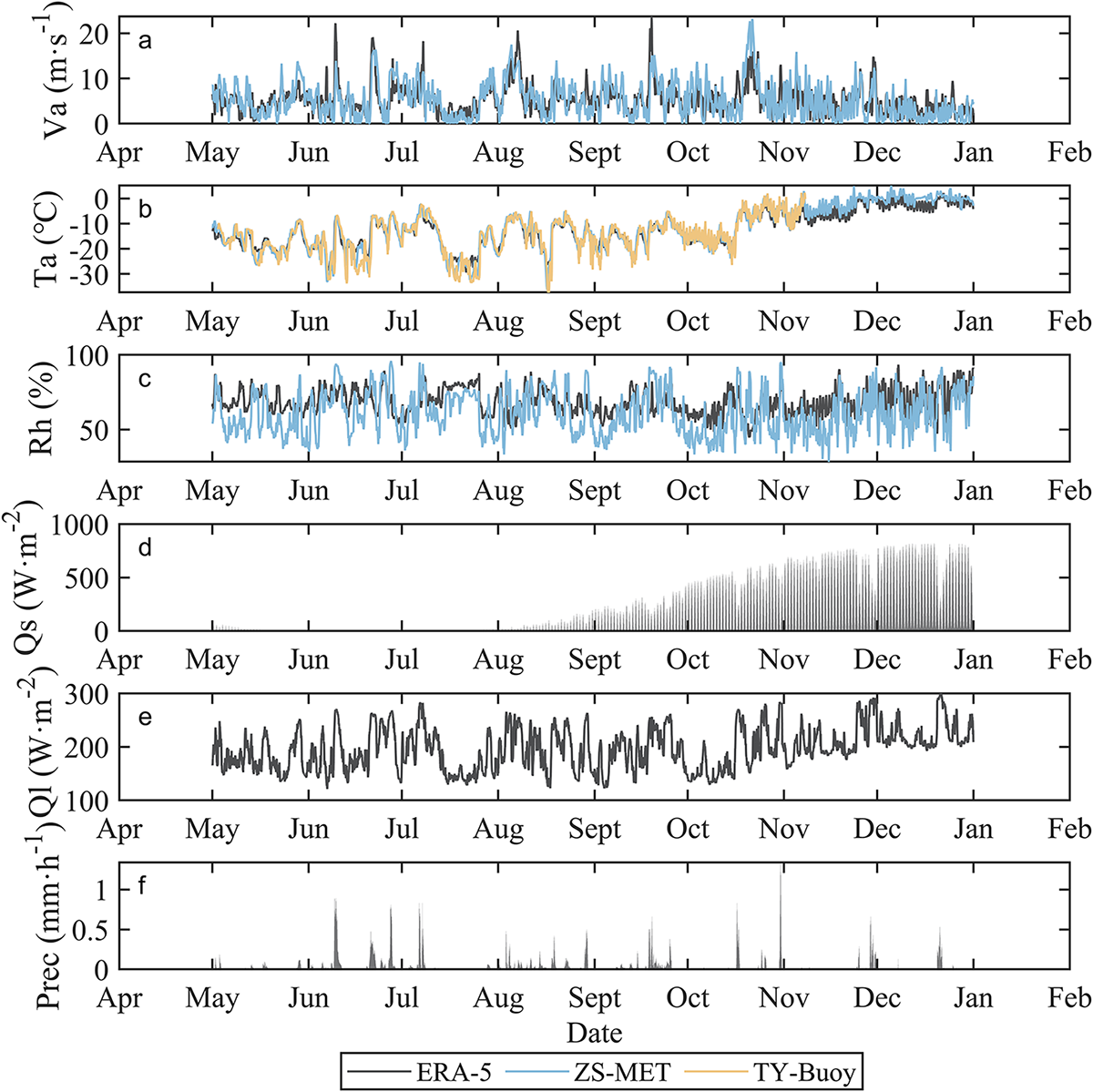
Figure A1. Time series of meteorological parameters applied for model experiments. The  ${V_a}$ ${T_a}$ and ${R_h}$ are AWS observations, and $Prec$, ${Q_s}$ and ${Q_l}$ are ERA5 results.
Table A1. Model parameters based on in situ observations and literature applied in this study
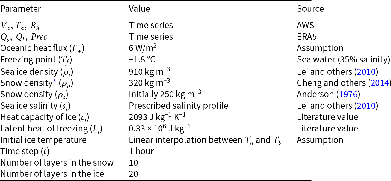
* Snow density used to convert precipitation to snow depth.


 Open access