


1. Introduction
We are concerned with extension of the powerful nonlinear steepest descent method due to Deift and Zhou [Reference Deift and Zhou8] (aka the Riemann-Hilbert problem approach) for the study of the long-time behaviour of the solution to the Cauchy problem for the Korteweg-de Vries (KdV) equation (see e.g. [Reference Ablowitz and Clarkson1],[Reference Novikov, Manakov, Pitaevskii and Zakharov20])
 \begin{equation}
\partial _{t}q-6q\partial _{x}q+\partial _{x}^{3}q=0,
\end{equation}
\begin{equation}
\partial _{t}q-6q\partial _{x}q+\partial _{x}^{3}q=0,
\end{equation} \begin{equation}
q\left( x,0\right) =q\left( x\right) ,
\end{equation}
\begin{equation}
q\left( x,0\right) =q\left( x\right) ,
\end{equation} with certain slowly decaying (long-range) initial profiles q. Note that [Reference Deift and Zhou8] deals with the modified KdV (mKdV) for  $q\left(
x\right) $ from the Schwarz class, which of course assumes rapid decay. A comprehensive treatment of the KdV case is offered in [Reference Grunert and Teschl12] where decay and smoothness assumptions are relaxed to
$q\left(
x\right) $ from the Schwarz class, which of course assumes rapid decay. A comprehensive treatment of the KdV case is offered in [Reference Grunert and Teschl12] where decay and smoothness assumptions are relaxed to
 \begin{equation}
\int_{\mathbb{R}}\left( 1+\left\vert x\right\vert \right) \left( \left\vert
q\left( x\right) \right\vert +\left\vert q^{\prime }\left( x\right)
\right\vert +\left\vert q^{\prime \prime }\left( x\right) \right\vert
+\left\vert q^{\prime \prime \prime }\left( x\right) \right\vert \right)
\mathrm{d}x \lt \infty \text{.}
\end{equation}
\begin{equation}
\int_{\mathbb{R}}\left( 1+\left\vert x\right\vert \right) \left( \left\vert
q\left( x\right) \right\vert +\left\vert q^{\prime }\left( x\right)
\right\vert +\left\vert q^{\prime \prime }\left( x\right) \right\vert
+\left\vert q^{\prime \prime \prime }\left( x\right) \right\vert \right)
\mathrm{d}x \lt \infty \text{.}
\end{equation}It seems plausible (but we do not have any reference) that conditions on the derivatives may be further relaxed at the expense of technical complications but the condition
 \begin{equation}
\int_{\mathbb{R}}\left( 1+\left\vert x\right\vert \right) \left\vert q\left(
x\right) \right\vert \mathrm{d}x \lt \infty\text{\ (short-range)},
\end{equation}
\begin{equation}
\int_{\mathbb{R}}\left( 1+\left\vert x\right\vert \right) \left\vert q\left(
x\right) \right\vert \mathrm{d}x \lt \infty\text{\ (short-range)},
\end{equation} is crucially important to run the underlying inverse scattering transform (IST) (see e.g. [Reference Marchenko and Iacob17]). In our [Reference Grudsky and Rybkin10],[Reference Rybkin21] we extend the IST to q’s with essentially arbitrary behavior at  $-\infty$ Footnote 1 but still require a sufficiently fast decay at $+\infty$. This should not come as a surprise since the KdV is a strongly unidirectional equation (solitons run to the right and radiation waves run to the left) which should translate into different contributions from the behavior of the data q at $\pm\infty$. We emphasize that relaxation of the condition (1.4) leads to a multitude of serious complications that can be resolved only in some particular cases and not surprisingly long-time asymptotic behaviour of the corresponding KdV solutions is out of reach in general. Our goal is to shed some light on this difficult situation but we need first to fix our terminology.
Associate with q the full line (self-adjoint) Schrodinger operator  $
\mathbb{L}_{q}=-\partial _{x}^{2}+q(x)$. For its spectrum
$
\mathbb{L}_{q}=-\partial _{x}^{2}+q(x)$. For its spectrum  $\sigma \left(
\mathbb{L}_{q}\right) $ we have
$\sigma \left(
\mathbb{L}_{q}\right) $ we have
 \begin{equation*}
\sigma \left( \mathbb{L}_{q}\right) =\sigma _{\mathrm{d}}\left( \mathbb{L}
_{q}\right) \cup \sigma _{\mathrm{ac}}\left( \mathbb{L}_{q}\right) \text{,}
\end{equation*}
\begin{equation*}
\sigma \left( \mathbb{L}_{q}\right) =\sigma _{\mathrm{d}}\left( \mathbb{L}
_{q}\right) \cup \sigma _{\mathrm{ac}}\left( \mathbb{L}_{q}\right) \text{,}
\end{equation*} where the discrete component  $\sigma _{\mathrm{d}}\left( \mathbb{L}
_{q}\right) =\{-\kappa _{n}^{2}\}$ is finite and for the absolutely continuous one has
$\sigma _{\mathrm{d}}\left( \mathbb{L}
_{q}\right) =\{-\kappa _{n}^{2}\}$ is finite and for the absolutely continuous one has  $\sigma _{\mathrm{ac}}\left( \mathbb{L}_{q}\right)
=[0,\infty )$. There is no positive singular continuous spectrum. The Schr ödinger equation
$\sigma _{\mathrm{ac}}\left( \mathbb{L}_{q}\right)
=[0,\infty )$. There is no positive singular continuous spectrum. The Schr ödinger equation
 \begin{equation}
\mathbb{L}_{q}\psi =k^{2}\psi,
\end{equation}
\begin{equation}
\mathbb{L}_{q}\psi =k^{2}\psi,
\end{equation} has two (linearly independent) Jost solutions  $\psi ^{\left( \pm \right)
}(x,k)$, i.e. solutions satisfying
$\psi ^{\left( \pm \right)
}(x,k)$, i.e. solutions satisfying
 \begin{equation}
\psi ^{\left( \pm \right) }(x,k)\sim \mathrm{e}^{\pm \mathrm{i}
kx},\;\partial _{x}\psi ^{\left( \pm \right) }(x,k)\sim \pm \mathrm{i}k\psi
^{\left( \pm \right) }(x,k),\text{\ \ }x\rightarrow \pm \infty ,
\end{equation}
\begin{equation}
\psi ^{\left( \pm \right) }(x,k)\sim \mathrm{e}^{\pm \mathrm{i}
kx},\;\partial _{x}\psi ^{\left( \pm \right) }(x,k)\sim \pm \mathrm{i}k\psi
^{\left( \pm \right) }(x,k),\text{\ \ }x\rightarrow \pm \infty ,
\end{equation} that are analytic in the upper half-plane and continuous to the real line. Since q is real,  $\overline{\psi ^{\left( +\right) }}$ also solves (1.5) and one can easily see that the pair
  $\{\psi ^{\left( +\right) },
\overline{\psi ^{\left( +\right) }}\}$ forms a fundamental set for (1.5). Hence
$\{\psi ^{\left( +\right) },
\overline{\psi ^{\left( +\right) }}\}$ forms a fundamental set for (1.5). Hence  $\psi ^{\left( -\right) }$ is a linear combination of
  $\{\psi
^{\left( +\right) },\overline{\psi ^{\left( +\right) }}\}$. We write this fact as follows (
$\{\psi
^{\left( +\right) },\overline{\psi ^{\left( +\right) }}\}$. We write this fact as follows ( $k\in \mathbb{R}$)
 \begin{equation}
T(k)\psi ^{\left( -\right) }(x,k)=\overline{\psi ^{\left( +\right) }(x,k)}
+R(k)\psi ^{\left( +\right) }(x,k),\text{(basic scattering identity)}
\end{equation}
\begin{equation}
T(k)\psi ^{\left( -\right) }(x,k)=\overline{\psi ^{\left( +\right) }(x,k)}
+R(k)\psi ^{\left( +\right) }(x,k),\text{(basic scattering identity)}
\end{equation}where T and R are called the transmission and (right) reflection coefficient respectively. The identity (1.7) is totally elementary but serves as a basis for inverse scattering theory. As is well-known (see, e.g. [Reference Marchenko and Iacob17]), the triple
 \begin{equation}
S_{q}=\{R,(\kappa _{n},c_{n})\},
\end{equation}
\begin{equation}
S_{q}=\{R,(\kappa _{n},c_{n})\},
\end{equation} where  $c_{n}=\left\Vert \psi ^{\left( +\right) }(\cdot ,\mathrm{i}\kappa
_{n})\right\Vert ^{-1}$, determines q uniquely and is called the scattering data for
$c_{n}=\left\Vert \psi ^{\left( +\right) }(\cdot ,\mathrm{i}\kappa
_{n})\right\Vert ^{-1}$, determines q uniquely and is called the scattering data for  $\mathbb{L}_{q}$.
Among initial data (aka potentials) that are not subject to (1.3) Wigner–von Neumann (WvN) type potentials
 \begin{equation}
q\left( x\right) =(A/x)\sin \left( 2\omega x+\delta \right) +O\left(
x^{-2}\right) ,x\rightarrow \pm \infty ,
\end{equation}
\begin{equation}
q\left( x\right) =(A/x)\sin \left( 2\omega x+\delta \right) +O\left(
x^{-2}\right) ,x\rightarrow \pm \infty ,
\end{equation} where  $A,\omega ,\delta $ are real constants, play a particularly important role due to their physical relevance. Note that q’s satisfying 1.9 are in L 2 and therefore, due to the famous Bourgain’s result [Reference Bourgain4], the Cauchy problem for the KdV equation (1.1)-(1.2) is well-posed. Moreover, the scattering theory can be developed along the same lines with its short-range counterpart except. The main feature of WvN type potentials is the important fact that if
  $
\gamma =\left\vert A/\left( 4\omega \right) \right\vert \gt 1/2$ then for some boundary condition at x = 0 the half-line Schrodinger operator with a potential of the form 1.9 has a positive bound state at energy ω 2. An explicit example to this effect was constructed in the seminal paper by WvN [Reference von Neumann and Winger25]. Certain q’s subject to 1.9 support a positive (embedded) bound state in the full line context (see e.g. [Reference Rybkin23] and the literature cited therein) but it is never the case for potentials restricted to a half-line. If ω 2 is not an embedded bound state then the energy ω 2 is commonly referred as to a WvN resonance. It is shown in [Reference Klaus14] that the Jost solutions
$
\gamma =\left\vert A/\left( 4\omega \right) \right\vert \gt 1/2$ then for some boundary condition at x = 0 the half-line Schrodinger operator with a potential of the form 1.9 has a positive bound state at energy ω 2. An explicit example to this effect was constructed in the seminal paper by WvN [Reference von Neumann and Winger25]. Certain q’s subject to 1.9 support a positive (embedded) bound state in the full line context (see e.g. [Reference Rybkin23] and the literature cited therein) but it is never the case for potentials restricted to a half-line. If ω 2 is not an embedded bound state then the energy ω 2 is commonly referred as to a WvN resonance. It is shown in [Reference Klaus14] that the Jost solutions  $\psi
^{\left( \pm \right) }(x,k)$ blow up to the order
$\psi
^{\left( \pm \right) }(x,k)$ blow up to the order  $\gamma =\left\vert
A/\left( 4\omega \right) \right\vert $ at ±ω and for this reason ω could be called a spectral singularity of order γ, the term that is more common in the soliton community. At such a point,
$\gamma =\left\vert
A/\left( 4\omega \right) \right\vert $ at ±ω and for this reason ω could be called a spectral singularity of order γ, the term that is more common in the soliton community. At such a point,  $
T\left( \pm \omega \right) =0$ and therefore [Reference Marchenko and Iacob17] one of the (necessary) condition guaranteeing that the triple (1.8) is indeed scattering data fails. Our interest in WvN potentials is inspired in part by the work of Matveev (see [Reference Matveev18] and the literature cited therein) and his proposal [Reference Dubard, Gaillard, Klein and Matveev9]: “A very interesting unsolved problem is to study the large time behaviour of the solutions to the KdV equation corresponding to the smooth initial data like
$
T\left( \pm \omega \right) =0$ and therefore [Reference Marchenko and Iacob17] one of the (necessary) condition guaranteeing that the triple (1.8) is indeed scattering data fails. Our interest in WvN potentials is inspired in part by the work of Matveev (see [Reference Matveev18] and the literature cited therein) and his proposal [Reference Dubard, Gaillard, Klein and Matveev9]: “A very interesting unsolved problem is to study the large time behaviour of the solutions to the KdV equation corresponding to the smooth initial data like  $cx^{-1}\sin 2kx$,
  $
c\in \mathbb{R}$. Depending on the choice of the constant c the related Schrödinger operator might have finite or infinite or zero number of the negative eigenvalues. The related inverse scattering problem is not yet solved and the study of the related large times evolution is a very challenging problem.” Note that what Matveev says about the negative spectrum is in fact an old result by Klaus [Reference Klaus15]: the potential
$
c\in \mathbb{R}$. Depending on the choice of the constant c the related Schrödinger operator might have finite or infinite or zero number of the negative eigenvalues. The related inverse scattering problem is not yet solved and the study of the related large times evolution is a very challenging problem.” Note that what Matveev says about the negative spectrum is in fact an old result by Klaus [Reference Klaus15]: the potential
 \begin{equation*}
q_{\gamma }=(A/x)\sin \left( 2\omega x+\delta \right),
\end{equation*}
\begin{equation*}
q_{\gamma }=(A/x)\sin \left( 2\omega x+\delta \right),
\end{equation*} has finite negative spectrum if  $\gamma =\left\vert A/\left( 4\omega \right)
\right\vert \lt \sqrt{1/2}$ but if
$\gamma =\left\vert A/\left( 4\omega \right)
\right\vert \lt \sqrt{1/2}$ but if  $\gamma \geq \sqrt{1/2}$ the negative spectrum (necessarily discrete) is infinite (accumulating to zero). Thus, if $\gamma \geq \sqrt{1/2}$ then the triple (1.8) also should include infinitely many arbitrary norming constants cn (Recall that a norming constant determines a soliton’s initial location).
While the Matveev problem is still a long shot, we have some partial results on the inverse scattering problem. Namely, in [Reference Grudsky and Rybkin11] we show that if γ is small enough (small coupling constant) the problem (1.1)-(1.2) can be solved by the IST (in fact, for a linear combination of WvN potentials). However, this good news for small WvN potentials does not yet imply applicability of the nonlinear steepest descent, which Matveev refers to as a “very challenging problem”. The main issue here is that WvN resonances cause the underlying Riemann-Hilbert problem (RHP) to become singular (and the standard conjugation step of RHP fails). Another issue is a poor understanding (as opposed to the classical case) of smoothness properties of R (at the origin in particular) which complicates the contour deformation step in RHP.
In this contribution we solely focus on the effect of WvN resonances on the KdV solution. We show that a WvN resonance gives rise to a new large-time asymptotic region  $x\sim -12\omega ^{2}t$ as $t\rightarrow +\infty $, which we call the resonance regime. To show this we adapt the nonlinear steepest descent to handle a certain singular RHP. In other words, we find a class of explicit initial data that produces one WvN resonance and is free of the IST issues associated with the long range nature of our initial data.
Our approach rests on [Reference Grunert and Teschl12], [Reference Krüger and Teschl16], and [Reference Budylin5]. We start out from the standard well-posed vector RHP, which we conjugate with the partial transmission coefficient. The latter lets us deform the conjugated RHP to the one with the jump matrix that is exponentially close to the identity matrix away from ±ω (in fact, without loss of generality, we can set ω = 1). This, in turn, allows us to reduce the original RHP to the one on small crosses centered at ±ω, which can be decoupled into two RHP at  $+\omega $ and $-\omega $. The solution to each of them reduces to the one centered at 0. We then replace the entries of the jump matrix on the small cross with their behaviors at 0 followed by extending the cross to infinity. So far we have followed [Reference Grunert and Teschl12], [Reference Krüger and Teschl16] with no change. However, since the partial transmission coefficient is unbounded at ±ω, the jump matrix of our RHP on the cross is unbounded (in [Reference Grunert and Teschl12], [Reference Krüger and Teschl16] it is bounded). It takes only a simple adjustment to the conjugation step from [Reference Grunert and Teschl12], [Reference Krüger and Teschl16] to reduce our singular RHP back to a matrixFootnote 2 RHP on the real line, which we call the model matrix RHP. As opposed to the classical situation of [Reference Grunert and Teschl12], [Reference Krüger and Teschl16], the jump matrix of our model RHP is not constant (and not even bounded) and cannot be explicitly solved in terms of parabolic cylinder functions. The classical approach however admits a modification which is suitably done in [Reference Budylin5]Footnote 3. The results of [Reference Budylin5] then yield the asymptotic of the solution to our model RHP (for large spectral variable), which is what is required to complete the derivation of our asymptotic formula (Theorem 3.3) following again [Reference Grunert and Teschl12].
Since it is a case study, we do not give here full detail leaving this for a future publication where our rather narrow class of potentials will be placed in a much broader class.
The paper is organized as follows. In Section 2, we fix our terminology and introduce our main ingredients. In Section 3, we state our main results. Section 4 is devoted to introducing our original RHP. In Section 5, we introduce the partial transmission coefficient and find its asymptotics around critical points that are crucially important to what follows. Section 6 is devoted to standard conjugation and deformation of our original RHP. In Section 7, we reduce our deformed RHP to a new matrix RHP on two small crosses centred at the critical points. In Section 8 we find asymptotics at the critical points of the jump matrix which allows us to reduce the RHP to a matrix one with the jump matrix on a single but infinite cross in Section 9. Section 10 deals with a second conjugation step where we transform the problem on a cross back to the problem on the real line. In Section 11, we solve the new problem on the real line by transforming it to an additive RHP. In Section 12, we finally prove Theorem 3.3. In the final section 13, we make some remarks on what we have not done.
2. Notation and auxiliaries
We follow standard notation accepted in complex analysis:  $\mathbb{C}$ is the complex plane,
  $\mathbb{C}^{\pm}=\left\{z\in\mathbb{C}:\pm\mathrm{Im}
z \gt 0\right\} $,
$\mathbb{C}^{\pm}=\left\{z\in\mathbb{C}:\pm\mathrm{Im}
z \gt 0\right\} $,  $\overline{z}$ is the complex conjugate of z.
Matrices (including rows and columns) are denoted by boldface letters; low/upper case being reserved for  $2\times 1$ (row vector) and $2\times 2$ matrix respectively with an exception for Pauli matrices which are traditionally denoted by
 \begin{equation*}
\sigma _{1}=\left(
\begin{array}{cc}
0 & 1 \\
1 & 0
\end{array}
\right) ,\ \ \ \sigma _{3}=\left(
\begin{array}{cc}
1 & 0 \\
0 & -1
\end{array}
\right) .
\end{equation*}
\begin{equation*}
\sigma _{1}=\left(
\begin{array}{cc}
0 & 1 \\
1 & 0
\end{array}
\right) ,\ \ \ \sigma _{3}=\left(
\begin{array}{cc}
1 & 0 \\
0 & -1
\end{array}
\right) .
\end{equation*} We write  $f\left( z\right) \sim g\left( z\right) ,\ $as
  $z\rightarrow z_{0}
\text{,}$ if
$z\rightarrow z_{0}
\text{,}$ if  $\lim\left( f\left( z\right) -g\left( z\right) \right) =0,~$as
  $
z\rightarrow z_{0}$. We use the standard big O notation when the rate needs to be specified.
$
z\rightarrow z_{0}$. We use the standard big O notation when the rate needs to be specified. $\log z$ is always defined with a cut along $\left( -\infty ,0\right) $. That is, $\mathrm{Im}\log z=\arg z\in (-\pi ,\pi ]$.
Given an oriented contour Γ, by  $z_{+}$ ( $z_{-}$) we denote the positive (negative) side of Γ. Recall that the positive (negative) side is the one that lies to the left (right) as one traverses the contour in the direction of the orientation. For a function $f\left( z\right) $ analytic in $\mathbb{C}\setminus \Gamma $, by $f_{+}(z),z\in \Gamma $, we denote the angular limit from above and by $f_{-}(z)$ the one from below. In particular, if $\Gamma =\mathbb{R}$ then
  $f_{\pm }\left( x\right) =f\left(
x\pm \mathrm{i}0\right) =\lim_{\varepsilon \rightarrow +0}f\left( x\pm
\mathrm{i}\varepsilon \right) ,x\in \mathbb{R}$.
$f_{\pm }\left( x\right) =f\left(
x\pm \mathrm{i}0\right) =\lim_{\varepsilon \rightarrow +0}f\left( x\pm
\mathrm{i}\varepsilon \right) ,x\in \mathbb{R}$.
Finally,  $\mathrm{1}_{S}$ is the characteristic function of a real set S.
3. Our class of initial data and main results
Our construction of initial data is based upon [Reference Rybkin24]. Consider the potential (it is not the one we will deal with yet)
 \begin{equation}
q_{0}\left( x\right) =\left\{
\begin{array}{cc}
-2\dfrac{\mathrm{d}^{2}}{\mathrm{d}x^{2}}\log \left\{1+a\left( \sin
2x-2x\right) \right\} , & x \lt 0 \\
0, & x\geq 0
\end{array}
\right. ,
\end{equation}
\begin{equation}
q_{0}\left( x\right) =\left\{
\begin{array}{cc}
-2\dfrac{\mathrm{d}^{2}}{\mathrm{d}x^{2}}\log \left\{1+a\left( \sin
2x-2x\right) \right\} , & x \lt 0 \\
0, & x\geq 0
\end{array}
\right. ,
\end{equation} where a is a positive number. One can easily see that the function q 0 is continuous and  $q_{0}\left( 0\right) =0$ but
  $q_{0}^{\prime }\left(
x\right) $ has a jump discontinuity at x = 0. Moreover,
$q_{0}^{\prime }\left(
x\right) $ has a jump discontinuity at x = 0. Moreover,
 \begin{equation}
q_{0}\left( x\right) =-4\ \dfrac{\sin 2x}{x}+O\left( \frac{1}{x^{2}}\right)
,\ \ x\rightarrow -\infty .
\end{equation}
\begin{equation}
q_{0}\left( x\right) =-4\ \dfrac{\sin 2x}{x}+O\left( \frac{1}{x^{2}}\right)
,\ \ x\rightarrow -\infty .
\end{equation} Note that the leading term is independent of a. Apparently,  $q_{0}\in
L^{2}\left( \mathbb{R}\right) $ but not even in
$q_{0}\in
L^{2}\left( \mathbb{R}\right) $ but not even in  $L^{1}\left( \mathbb{R}
\right) $. Thus, q 0 is not short-range. Also note that
$L^{1}\left( \mathbb{R}
\right) $. Thus, q 0 is not short-range. Also note that
 \begin{equation*}
\int_{-\infty }^{\infty }q_{0}\left( x\right) \mathrm{d}x=0.
\end{equation*}
\begin{equation*}
\int_{-\infty }^{\infty }q_{0}\left( x\right) \mathrm{d}x=0.
\end{equation*} The main feature of q 0 is that  $\mathbb{L}_{q_{0}}$ admits an explicit spectral and scattering theory. The Schrödinger operator
  $\mathbb{L}
_{q_{0}}$ on
$\mathbb{L}
_{q_{0}}$ on  $L^{2}\left( \mathbb{R}\right) $ with q 0 given by (3.1) has the following properties:
• The spectrum
 $\sigma \left( \mathbb{L}_{q_{0}}\right) =\left\{-\kappa
^{2}\right\} \cup \sigma _{\mathrm{ac}}\left( \mathbb{L}_{q_{0}}\right) $ and
$\sigma _{\mathrm{ac}}\left( \mathbb{L}_{q_{0}}\right) $ is two fold purely absolutely purely continuous filling
$[0,\infty )$. Here κ > 0 solves the equation
(3.3)\begin{equation}
\kappa ^{3}+\kappa =2a.
\end{equation}
$\sigma \left( \mathbb{L}_{q_{0}}\right) =\left\{-\kappa
^{2}\right\} \cup \sigma _{\mathrm{ac}}\left( \mathbb{L}_{q_{0}}\right) $ and
$\sigma _{\mathrm{ac}}\left( \mathbb{L}_{q_{0}}\right) $ is two fold purely absolutely purely continuous filling
$[0,\infty )$. Here κ > 0 solves the equation
(3.3)\begin{equation}
\kappa ^{3}+\kappa =2a.
\end{equation}• The left Jost solution
$\psi \left( x,k\right) $ given by
(3.4)\begin{equation}
\psi \left( x,k\right) =\mathrm{e}^{-\mathrm{i}kx}\left\{1+\left( \frac{
\mathrm{e}^{\mathrm{i}x}}{k-1}-\frac{\mathrm{e}^{-\mathrm{i}x}}{k+1}\right)
\frac{2a\sin x}{1-2ax+a\sin 2x}\right\} ,\ \ \ x \lt 0,
\end{equation}is a meromorphic function with two simple poles at ±1 (therefore ±1 are spectral singularities of order 1).
• The (right) reflection coefficient R 0 and the transmission coefficient T 0 are rational functions given by
(3.5)\begin{equation}
T^{0}\left( k\right) =\frac{k^{3}-k}{k^{3}-k+2\mathrm{i}a},\ \ R^{0}\left(
k\right) =\frac{-2\mathrm{i}a}{k^{3}-k+2\mathrm{i}a},
\end{equation}


It is convenient to remove the negative bound state  $-\kappa ^{2}$ by applying a single Darboux transformation (see e.g. [Reference Deift and Trubowitz6]). This way one gets a new potential
 \begin{equation*}
q\left( x\right) =q_{0}\left( x\right) -2\dfrac{\mathrm{d}^{2}}{\mathrm{d}
x^{2}}\log \psi \left( x,\mathrm{i}\kappa \right),
\end{equation*}
\begin{equation*}
q\left( x\right) =q_{0}\left( x\right) -2\dfrac{\mathrm{d}^{2}}{\mathrm{d}
x^{2}}\log \psi \left( x,\mathrm{i}\kappa \right),
\end{equation*} where ψ is given by (3.4). Since the single Darboux transformation preserves support,  $q\left( x\right) $ can be simplified to read
 \begin{equation}
q\left( x\right) =\left\{
\begin{array}{cc}
-2\dfrac{\mathrm{d}^{2}}{\mathrm{d}x^{2}}\log \left\{1-\left( \kappa
^{3}+\kappa \right) x+\left( \kappa ^{3}-\kappa \right) \sin x\cos x+2\kappa
^{2}\sin ^{2}x\right\} , & x \lt 0 \\
0, & x\geq 0
\end{array}
\right. ,
\end{equation}
\begin{equation}
q\left( x\right) =\left\{
\begin{array}{cc}
-2\dfrac{\mathrm{d}^{2}}{\mathrm{d}x^{2}}\log \left\{1-\left( \kappa
^{3}+\kappa \right) x+\left( \kappa ^{3}-\kappa \right) \sin x\cos x+2\kappa
^{2}\sin ^{2}x\right\} , & x \lt 0 \\
0, & x\geq 0
\end{array}
\right. ,
\end{equation}where κ is a positive number related to a by 3.3. The scattering quantities transform as follows
 \begin{equation*}
T\left( k\right) =\frac{k-\mathrm{i}\kappa }{k+\mathrm{i}\kappa }T^{0}\left(
k\right) ,\ \ \ R\left( k\right) =-\frac{k-\mathrm{i}\kappa }{k+\mathrm{i}
\kappa }R^{0}\left( k\right) .
\end{equation*}
\begin{equation*}
T\left( k\right) =\frac{k-\mathrm{i}\kappa }{k+\mathrm{i}\kappa }T^{0}\left(
k\right) ,\ \ \ R\left( k\right) =-\frac{k-\mathrm{i}\kappa }{k+\mathrm{i}
\kappa }R^{0}\left( k\right) .
\end{equation*}For the reader’s convenience we summarize important properties of q’s in the following
Theorem 3.1. The Schrödinger operator  $\mathbb{L}_{q}$ on
  $
L^{2}\left( \mathbb{R}\right) $ with q given by (3.1) has the properties:
$
L^{2}\left( \mathbb{R}\right) $ with q given by (3.1) has the properties:
(1) (Spectrum)
$\sigma \left( \mathbb{L}_{q}\right) =\sigma _{\mathrm{ac}
}\left( \mathbb{L}_{q}\right) $
$=[0,\infty )$ and multiplicity two. The point 1 is a first order WvN resonance.(2) (Scattering quantities) The transmission coefficient T and the (right) reflection coefficient R are rational functions given by
(3.7)\begin{equation}
\begin{array}{ccccc}
T\left( k\right) & = & \dfrac{k-\mathrm{i}\kappa }{k+\mathrm{i}\kappa }
\dfrac{k^{3}-k}{k^{3}-k+2\mathrm{i}a} & = & \dfrac{k^{3}-k}{\left( k+\mathrm{
i}\kappa \right) \left( k-k_{-}\right) \left( k-k_{+}\right) } \\
R\left( k\right) & = & \dfrac{k-\mathrm{i}\kappa }{k+\mathrm{i}\kappa }
\dfrac{2\mathrm{i}a}{k^{3}-k+2\mathrm{i}a} & = & \dfrac{\mathrm{i}\left(
\kappa ^{3}+\kappa \right) }{\left( k+\mathrm{i}\kappa \right) \left(
k-k_{-}\right) \left( k-k_{+}\right) }
\end{array}
,
\end{equation}where
\begin{equation*}
k_{\pm }=\pm \sqrt{1+3\kappa ^{2}/4}-\mathrm{i}\kappa /2.
\end{equation*}(3) (Asymptotic behavior)
$q\left( x\right) $ has the asymptotic behavior
(3.8)\begin{equation}
q\left( x\right) =-4\ \dfrac{\sin\left( 2x+\delta\right) }{x}+O\left( \frac{1
}{x^{2}}\right) ,\ \ x\rightarrow-\infty,
\end{equation}where
\begin{equation*}
\tan\delta=\frac{2\kappa}{1-\kappa^{2}}.
\end{equation*}


Remark 3.2. Observe that since the left L and right R reflection coefficient are related by  $L=-\left( T/\overline{T}\right) \overline{R}$, one readily sees from (3.7) that L = R. Note the potential $q\left( -x\right) $ has the same transition coefficients 3.7 and hence
  $q\left(
x\right) $ and
$q\left(
x\right) $ and  $q\left( -x\right) $ share the same scattering matrix meaning that the set $S_{q}=\left\{R\right\} $ does not make up scattering data. This phenomenon was first observed in [Reference Abraham, DeFacio and Moses3] for certain potentials decaying as $O\left( x^{-2}\right) $. We mention that the construction in [Reference Abraham, DeFacio and Moses3] involves a delta-function whereas our counterexample is given by a continuous function. Note that the uniqueness is restored once we a priori assume that $q\left( x\right) $ is supported on
  $\left( -\infty
,0\right) $.
$\left( -\infty
,0\right) $.
Note that γ = 1 for any q of the form (3.6) and thus the results of [Reference Rybkin24] do not apply as we need  $\gamma \lt 1/2$. However since the support of each q is restricted to $\left( -\infty,0\right) $ the IST does apply [Reference Rybkin22] and, as in the classical IST, the time evolved scattering data for the whole class is given by
 \begin{equation}
S_{q}(t)=\left\{R(k)\exp\left( 8\mathrm{i}k^{3}t\right) \right\}.
\end{equation}
\begin{equation}
S_{q}(t)=\left\{R(k)\exp\left( 8\mathrm{i}k^{3}t\right) \right\}.
\end{equation} The general theory [Reference Rybkin22] implies that  $q\left( x,t\right) $ is meromorphic in x on the whole complex plane for any t > 0. Moreover, for each fixed t > 0, $q\left( x,t\right) $ decays exponentially as
  $
x\rightarrow+\infty$ and behaves as 3.8 at
$
x\rightarrow+\infty$ and behaves as 3.8 at  $
-\infty$ [Reference Novikov and Khenkin19]. We now state our main result.
$
-\infty$ [Reference Novikov and Khenkin19]. We now state our main result.
Theorem 3.3 (On resonance asymptotic regime)
Let q(x) be of the form (3.6) with some positive κ. Then the solution  $q\left( x,t\right) $ to the KdV equation with the initial data $q\left( x\right) $ behaves along the line
  $
x=-12t$ as follows
$
x=-12t$ as follows
 \begin{eqnarray}
\left. q\left( x,t\right) \right\vert _{x=-12t} &\sim &\sqrt{\frac{4\nu
\left( t\right) }{3t}}\sin \left\{16t-\nu \left( t\right) \left[ 1+\pi \nu
\left( t\right) -\log \nu \left( t\right) \right] +\delta \right\} ,
\nonumber \\
t &\rightarrow &+\infty ,
\end{eqnarray}
\begin{eqnarray}
\left. q\left( x,t\right) \right\vert _{x=-12t} &\sim &\sqrt{\frac{4\nu
\left( t\right) }{3t}}\sin \left\{16t-\nu \left( t\right) \left[ 1+\pi \nu
\left( t\right) -\log \nu \left( t\right) \right] +\delta \right\} ,
\nonumber \\
t &\rightarrow &+\infty ,
\end{eqnarray}where
 \begin{equation*}
\nu \left( t\right) =\left( 1/2\pi \right) \log \left( 12\left( \kappa
^{3}+\kappa \right) ^{2}t\right),
\end{equation*}
\begin{equation*}
\nu \left( t\right) =\left( 1/2\pi \right) \log \left( 12\left( \kappa
^{3}+\kappa \right) ^{2}t\right),
\end{equation*}and a constant phase δ is given by
 \begin{align*}
\delta & =\frac{2}{\pi }\int\limits_{0}^{1}\log \left\vert \frac{
T(s)/T^{\prime }\left( 1\right) }{1-s}\right\vert ^{2}\frac{\mathrm{d}s}{
1-s^{2}}-\frac{2}{\pi }\int\limits_{0}^{1}\frac{\log s{\mathrm{d}s}}{s-2}. \\
& +\frac{1}{\pi }\log \frac{\kappa ^{3}+\kappa }{2}\log \frac{\kappa
^{3}+\kappa }{8}+\arctan \frac{2\kappa }{1-\kappa ^{2}}-\frac{\pi }{3}.
\end{align*}
\begin{align*}
\delta & =\frac{2}{\pi }\int\limits_{0}^{1}\log \left\vert \frac{
T(s)/T^{\prime }\left( 1\right) }{1-s}\right\vert ^{2}\frac{\mathrm{d}s}{
1-s^{2}}-\frac{2}{\pi }\int\limits_{0}^{1}\frac{\log s{\mathrm{d}s}}{s-2}. \\
& +\frac{1}{\pi }\log \frac{\kappa ^{3}+\kappa }{2}\log \frac{\kappa
^{3}+\kappa }{8}+\arctan \frac{2\kappa }{1-\kappa ^{2}}-\frac{\pi }{3}.
\end{align*}By way of discussing this theorem we offer some comments.
Remark 3.4. The class of initial data of the form 3.6 appears extraordinarily narrow. But of course by a simple rescaling we can place the resonance at any point ω 2. Secondly, 3.6 shares the same asymptotic behaviour as any WvN type potential with γ = 1 restricted to  $\left( -\infty ,0\right) $ but have explicit rational scattering data, which has significant technical advantages.
Remark 3.5. It is shown in [Reference Novikov and Khenkin19] that simple zeros of the transmission coefficient are always associated with the behaviour 1.9 with γ = 1. The approach is based upon the Gelfand–Levitan–Marchenko equation and does not yield the existence of the resonance regime. Incidentally, the very concept of WvN resonance (nor spectral singularity to this matter) is not used in [Reference Novikov and Khenkin19].
Remark 3.6. Recall that in the short-range case the behaviour of  $\left. q\left(
x,t\right) \right\vert _{x=-ct}$ as
$\left. q\left(
x,t\right) \right\vert _{x=-ct}$ as  $t\rightarrow +\infty $ looks similar to 3.10 for any c > 0 (the similarity region) with one main difference: ν is constant. Thus, as opposed to the classical case where any radiant wave decays as $O\left( t^{-1/2}\right) $ when $t\rightarrow \infty $, our initial date (3.6) give rise to a radiant wave that decays as $O\left( \left( \log t/t\right) ^{1/2}\right) $. We believe that it is a new phenomenon that holds for any initial data producing zero transmission (full reflection) at some isolated positive energies.
Remark 3.7. In the NLS context, asymptotic regions related to spectral singularities are studied in [Reference Ablowitz and Segur2],[Reference Budylin5],[Reference Kamvissis13] by different methods. It follows from [Reference Ablowitz and Segur2] that for the focusing NLS a spectral singularity opens a new asymptotic region where the amplitude decays as  $
O\left( \left( \log t/t\right) ^{1/2}\right) $ and the phase includes
$
O\left( \left( \log t/t\right) ^{1/2}\right) $ and the phase includes  $\log
^{2}t$ term (similar to our resonance regime). The part of the paper [Reference Ablowitz and Segur2] devoted to the NLS has no proofs and is revisited in [Reference Kamvissis13] where it is claimed that the amplitude in [Reference Ablowitz and Segur2] is off by a multiplicative constant and the phase has no
$\log
^{2}t$ term (similar to our resonance regime). The part of the paper [Reference Ablowitz and Segur2] devoted to the NLS has no proofs and is revisited in [Reference Kamvissis13] where it is claimed that the amplitude in [Reference Ablowitz and Segur2] is off by a multiplicative constant and the phase has no  $\log ^{2}t$ term. The de-focusing case is considered in [Reference Budylin5] where the results also suggest the appearance of a new asymptotic region with the amplitude behaving like $O\left( \left( \log t/t\right) ^{1/2}\right) $ and the phase containing a $\log ^{2}t$ term. The paper [Reference Budylin5] relies on totally different arguments and the author appears to be unaware of [Reference Ablowitz and Segur2] and [Reference Kamvissis13]. It appears that there is no clarity on the issue and we hope to address it elsewhere.
Remark 3.8. In the short-range case, generically ,  $T\left( 0\right) =0$ (i.e.
  $T\left(
0\right) \neq 0$ only for some exceptional potentials). As it is shown in [Reference Ablowitz and Segur2],[Reference Deift, Venakides and Zhou7], the latter gives rise to a new asymptotic regime, called the collisionless shock region. We referee the interested reader to [Reference Ablowitz and Segur2],[Reference Deift, Venakides and Zhou7] and only mention here that
$T\left(
0\right) \neq 0$ only for some exceptional potentials). As it is shown in [Reference Ablowitz and Segur2],[Reference Deift, Venakides and Zhou7], the latter gives rise to a new asymptotic regime, called the collisionless shock region. We referee the interested reader to [Reference Ablowitz and Segur2],[Reference Deift, Venakides and Zhou7] and only mention here that  $\left(
x,t\right) $ in this region are no longer on a ray and the wave amplitude decays as
$\left(
x,t\right) $ in this region are no longer on a ray and the wave amplitude decays as  $O\left( \left( \log t/t\right) ^{2/3}\right) $ as
  $t\rightarrow
+\infty .$
$t\rightarrow
+\infty .$
4. Original RHP
As is always done in the RHP approach to the IST, we rewrite the (time evolved) basic scattering identity (1.7) as a vector RHP. To this end, introduce a  $2\times 1$ row vector
 \begin{equation}
\mathbf{m}(k,x,t)=\left\{
\begin{array}{c@{\quad}l}
\begin{pmatrix}
T(k)m^{\left( -\right) }(k,x,t) & m^{\left( +\right) }(k,x,t)
\end{pmatrix}
, & \mathrm{Im}k \gt 0, \\
\begin{pmatrix}
m^{\left( +\right) }(-k,x,t) & T(-k)m^{\left( -\right) }(-k,x,t)
\end{pmatrix}
, & \mathrm{Im}k \lt 0,
\end{array}
\right.
\end{equation}
\begin{equation}
\mathbf{m}(k,x,t)=\left\{
\begin{array}{c@{\quad}l}
\begin{pmatrix}
T(k)m^{\left( -\right) }(k,x,t) & m^{\left( +\right) }(k,x,t)
\end{pmatrix}
, & \mathrm{Im}k \gt 0, \\
\begin{pmatrix}
m^{\left( +\right) }(-k,x,t) & T(-k)m^{\left( -\right) }(-k,x,t)
\end{pmatrix}
, & \mathrm{Im}k \lt 0,
\end{array}
\right.
\end{equation}where
 \begin{equation}
m^{\left( \pm \right) }(k;x,t):=\mathrm{e}^{\mp \mathrm{i}kx}\psi ^{\left(
\pm \right) }(x,t;k),\text{ (Faddeev functions).}
\end{equation}
\begin{equation}
m^{\left( \pm \right) }(k;x,t):=\mathrm{e}^{\mp \mathrm{i}kx}\psi ^{\left(
\pm \right) }(x,t;k),\text{ (Faddeev functions).}
\end{equation} Note that we list k as the first variable as from now on it will be the main variable, the parameters  $\left( x,t\right) $ being often suppressed. Existence of $\psi ^{\left( \pm \right) }(x,t;k)$ for t > 0 follows from considerations given in [Reference Novikov and Khenkin19]. Also, since poles of
  $\psi
^{\left( -\right) }$ are cancelled by the zeros of T, we conclude that m is bounded on the whole complex plane. Details will be provided elsewhere for a much wider class of initial data.
$\psi
^{\left( -\right) }$ are cancelled by the zeros of T, we conclude that m is bounded on the whole complex plane. Details will be provided elsewhere for a much wider class of initial data.
Introduce the short hand notation
 \begin{equation*}
\xi\left( k\right) =\exp\left\{\mathrm{i}t\Phi\left( k\right) \right\} ,\
\Phi\left( k\right) =4k^{3}+\left( x/t\right) k,\ \ x\in\mathbb{R},t\geq0.
\end{equation*}
\begin{equation*}
\xi\left( k\right) =\exp\left\{\mathrm{i}t\Phi\left( k\right) \right\} ,\
\Phi\left( k\right) =4k^{3}+\left( x/t\right) k,\ \ x\in\mathbb{R},t\geq0.
\end{equation*}We treat m as a solution to
RHP#0. (Original RHP) Find a  $1\times2$ matrix (row) valued function $\mathbf{m}\left( k\right) $ which is analytic and bounded on
  $
\mathbb{C\diagdown R}$ and satisfies:
$
\mathbb{C\diagdown R}$ and satisfies:
(1) The jump condition
 \begin{equation}
\mathbf{m}_{+}\left( k\right) =\mathbf{m}_{-}\left( k\right) \mathbf{V}
\left( k\right) \text{for }k\in \mathbb{R},
\end{equation}
\begin{equation}
\mathbf{m}_{+}\left( k\right) =\mathbf{m}_{-}\left( k\right) \mathbf{V}
\left( k\right) \text{for }k\in \mathbb{R},
\end{equation} where  $\mathbf{m}_{\pm }\left( k\right) :=\mathbf{m}\left( k\pm \mathrm{i}
0\right) ,\ k\in \mathbb{R}$,
$\mathbf{m}_{\pm }\left( k\right) :=\mathbf{m}\left( k\pm \mathrm{i}
0\right) ,\ k\in \mathbb{R}$,
 \begin{equation}
\mathbf{V}\left( k\right) =\left(
\begin{array}{cc}
1-\left\vert R\left( k\right) \right\vert ^{2} & -\overline{R}\left(
k\right) \xi \left( k\right) ^{-2} \\
R\left( k\right) \xi \left( k\right) ^{2} & 1
\end{array}
\right) ,\text{(jump matrix),}
\end{equation}
\begin{equation}
\mathbf{V}\left( k\right) =\left(
\begin{array}{cc}
1-\left\vert R\left( k\right) \right\vert ^{2} & -\overline{R}\left(
k\right) \xi \left( k\right) ^{-2} \\
R\left( k\right) \xi \left( k\right) ^{2} & 1
\end{array}
\right) ,\text{(jump matrix),}
\end{equation}and R is given by 3.7;
(2) The symmetry condition
 \begin{equation*}
\mathbf{m}\left( -k\right) =\mathbf{m}\left( k\right) \sigma_{1}\text{;}
\end{equation*}
\begin{equation*}
\mathbf{m}\left( -k\right) =\mathbf{m}\left( k\right) \sigma_{1}\text{;}
\end{equation*}(3) The normalization condition
 \begin{equation*}
\mathbf{m}\left( k\right) \sim \left(
\begin{array}{cc}
1 & 1
\end{array}
\right) ,\ \ \ k\rightarrow \infty .
\end{equation*}
\begin{equation*}
\mathbf{m}\left( k\right) \sim \left(
\begin{array}{cc}
1 & 1
\end{array}
\right) ,\ \ \ k\rightarrow \infty .
\end{equation*}The solution to the initial problem 1.1-1.2 can then be found by
 \begin{equation}
q\left( x,t\right) =2\lim k^{2}\left( m_{1}\left( k,x,t\right) m_{2}\left(
k,x,t\right) -1\right) ,\ \ \ k\rightarrow\infty
\end{equation}
\begin{equation}
q\left( x,t\right) =2\lim k^{2}\left( m_{1}\left( k,x,t\right) m_{2}\left(
k,x,t\right) -1\right) ,\ \ \ k\rightarrow\infty
\end{equation} where  $m_{1,2}$ are the entries of m (see e.g. [Reference Grunert and Teschl12]).
The RHP approach is specifically robust (among others) in asymptotics analysis of  $\mathbf{m}\left( k;x,t\right) $ as $t\rightarrow +\infty $ in different asymptotic regions [Reference Grunert and Teschl12]. But it works well if the stationary point $k_{0}=\sqrt{-x/12t}$ of $\Phi \left( k\right) $ is not a real zero of $T\left( k\right) $. Recall that in the short-range case the only real zero of $T\left( k\right) $ is k = 0 and does not create any problems as long as $k_{0}\neq 0$. As already mentioned, the case of
  $
k_{0}=0 $ is considered in [Reference Deift, Venakides and Zhou7]. Note however that 0 is the left end point of the absolutely continuous spectrum, which is essential for the approach to work.
$
k_{0}=0 $ is considered in [Reference Deift, Venakides and Zhou7]. Note however that 0 is the left end point of the absolutely continuous spectrum, which is essential for the approach to work.
Remark 4.1. There is no problem with the well-posedness of RHP#0 and no problem with the deformation step as V is a meromorphic function on the entire plane. But there is a problem with adjusting the classical nonlinear steepest descent [Reference Deift and Zhou8]. Recall that in the mKdV case treated in [Reference Deift and Zhou8] we always have  $\left\vert R(k)\right\vert \lt 1$ and hence $R(k)/(1-|R(k)|^{2})$ can be approximated by analytic functions in the $L^{\infty}$ norm. As we have seen already, it is not our case and it appears to be a good open question how to adjust the nonlinear steepest descent to RHP#0.
Remark 4.2. RHP#0 does not appear singular so far. Its singularity will be clear below.
5. Partial transmission coefficient
In this section we study what is commonly referred to as the partial transmission coefficient, which plays the crucial role in the conjugation step discussed below. Following [Reference Grunert and Teschl12] we introduce it by
 \begin{equation*}
T(k,k_{0})=\exp\int\limits_{\left( -k_{0},k_{0}\right) }\frac{\log |T(s)|^{2}
}{s-k}\frac{{\mathrm{d}s}}{2\pi\mathrm{i}}.
\end{equation*}
\begin{equation*}
T(k,k_{0})=\exp\int\limits_{\left( -k_{0},k_{0}\right) }\frac{\log |T(s)|^{2}
}{s-k}\frac{{\mathrm{d}s}}{2\pi\mathrm{i}}.
\end{equation*} Since we are only concerned with the asymptotics related to the resonance region we take  $k_{0}=1$ and denote
 \begin{equation}
T_{0}\left( k\right) =T(k,1)=\exp\int\limits_{\left( -1,1\right) }\frac{
\log|T(s)|^{2}}{s-k}\frac{{\mathrm{d}s}}{2\pi\mathrm{i}}.
\end{equation}
\begin{equation}
T_{0}\left( k\right) =T(k,1)=\exp\int\limits_{\left( -1,1\right) }\frac{
\log|T(s)|^{2}}{s-k}\frac{{\mathrm{d}s}}{2\pi\mathrm{i}}.
\end{equation} If  $k_{0}=+\infty$ then $T\left( k,+\infty\right) $ returns the (full) transmission coefficient $T\left( k\right) $. $T_{0}(k)$ is clearly an analytic function for
  $k\in \mathbb{C}\backslash
\left[ -1,1\right] $. The following statement extends that of [Reference Grunert and Teschl12].
$k\in \mathbb{C}\backslash
\left[ -1,1\right] $. The following statement extends that of [Reference Grunert and Teschl12].
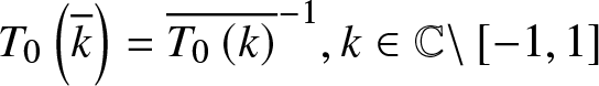
Theorem 5.1 The partial transmission coefficient  $T_{0}(k)$ satisfies the jump condition
 \begin{equation}
T_{0+}(k)=T_{0-}(k)(1-\left\vert R(k)\right\vert ^{2}),\ \ k\in \left(
-1,1\right),
\end{equation}
\begin{equation}
T_{0+}(k)=T_{0-}(k)(1-\left\vert R(k)\right\vert ^{2}),\ \ k\in \left(
-1,1\right),
\end{equation}and
(1)
$T_{0}(-k)=T_{0}(k)^{-1}$,
$T_{0}\left( \overline{k}\right) =\overline{
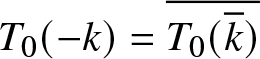
T_{0}\left( k\right) }^{-1},k\in\mathbb{C}\backslash\left[ -1,1\right] $;(2)
$T_{0}(-k)=\overline{T_{0}(\overline{k})}$,
$k\in\mathbb{C}$, in particular
$T_{0}(k)$ is real for
$k\in$i
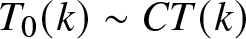
$\mathbb{R}$;(3) the behaviour near k = 0 is given by
$T_{0}(k)\sim CT(k)$ with C ≠ 0 for
$\mathrm{Im}k\geq0$;(4)
$T_{0}\left( k\right) $ can be factored out as
(5.3)\begin{equation}
T_{0}\left( k\right) =T_{0}^{\left( \mathrm{reg}\right) }\left( k\right)
T_{0}^{\left( \mathrm{sng}\right) }\left( k\right) ,
\end{equation}where the regular part
\begin{equation*}
T_{0}^{\left( \mathrm{reg}\right) }\left( k\right) =\frac{{k}}{\pi \mathrm{i}
}\int\limits_{0}^{1}\log \left\vert \frac{T(s)/\left( 1-s\right) }{T^{\prime
}\left( 1\right) }\right\vert ^{2}\frac{\mathrm{d}s}{s^{2}-k^{2}}
\end{equation*}is continuously differentiable at
$k=\pm 1$, and the singular part
(5.4)\begin{equation}
T_{0}^{\left( \mathrm{sng}\right) }\left( k\right) =\left( \frac{k-1}{k+1}
\right) ^{\mathrm{i}\nu }\exp \left\{k\int_{0}^{1}\frac{\log \left(
1-s\right) ^{2}}{s^{2}-k^{2}}\frac{\mathrm{d}s}{\pi \mathrm{i}}\right\} ,
\end{equation}(5.5)\begin{equation}
\nu :=-\left( 1/\pi \right) \log \left\vert T^{\prime }\left( 1\right)
\right\vert =\left( 1/\pi \right) \log a.
\end{equation}Moreover,
(5.6)\begin{equation}
T_{0}\left( k\right) \sim A_{0}\exp \left\{\mathrm{i}\nu \log \left(
k-1\right) +\frac{1}{2\mathrm{i}\pi }\log ^{2}\left( k-1\right) \right\}
,k\rightarrow 1,
\end{equation}where A 0 is a unimodular constant given by
(5.7)\begin{equation}
A_{0}=\exp \frac{\mathrm{i}}{\pi }\left\{\int\limits_{0}^{1}\log \left\vert
\frac{T(s)/T^{\prime }\left( 1\right) }{1-s}\right\vert ^{2}\frac{\mathrm{d}s
}{1-s^{2}}-\pi \nu \log 2-\frac{\pi ^{2}}{6}-\int\limits_{0}^{1}\frac{\log s{
\mathrm{d}s}}{s-2}\right\} .
\end{equation}


Proof. The items (1)-(3) are straightforward to check. Item (4) is a bit technical. Since  $\left\vert T\left( s\right) \right\vert $ is even, we clearly have
 \begin{align*}
\int\limits_{-1}^{1}\frac{\log |T(s)|^{2}}{s-k}{\mathrm{d}s}& {=2k}
\int\limits_{0}^{1}\frac{\log |T(s)|^{2}}{s^{2}-k^{2}}{\mathrm{d}s} \\
& ={2k}\int\limits_{0}^{1}\frac{\log |T(s)/\left( 1-s\right) |^{2}}{
s^{2}-k^{2}}{\mathrm{d}s+2k}\int\limits_{0}^{1}\frac{\log \left( 1-s\right)
^{2}}{s^{2}-k^{2}}{\mathrm{d}s}
\end{align*}
\begin{align*}
\int\limits_{-1}^{1}\frac{\log |T(s)|^{2}}{s-k}{\mathrm{d}s}& {=2k}
\int\limits_{0}^{1}\frac{\log |T(s)|^{2}}{s^{2}-k^{2}}{\mathrm{d}s} \\
& ={2k}\int\limits_{0}^{1}\frac{\log |T(s)/\left( 1-s\right) |^{2}}{
s^{2}-k^{2}}{\mathrm{d}s+2k}\int\limits_{0}^{1}\frac{\log \left( 1-s\right)
^{2}}{s^{2}-k^{2}}{\mathrm{d}s}
\end{align*}and therefore
 \begin{equation*}
T_{0}\left( k\right) =\exp \left\{k\int\limits_{0}^{1}\frac{\log
|T(s)/\left( 1-s\right) )|^{2}}{s^{2}-k^{2}}\frac{{\mathrm{d}s}}{\pi \mathrm{
i}}\right\} \exp \left\{k\int\limits_{0}^{1}\frac{\log \left( 1-s\right)
^{2}}{s^{2}-k^{2}}\frac{{\mathrm{d}s}}{\pi \mathrm{i}}\right\} .
\end{equation*}
\begin{equation*}
T_{0}\left( k\right) =\exp \left\{k\int\limits_{0}^{1}\frac{\log
|T(s)/\left( 1-s\right) )|^{2}}{s^{2}-k^{2}}\frac{{\mathrm{d}s}}{\pi \mathrm{
i}}\right\} \exp \left\{k\int\limits_{0}^{1}\frac{\log \left( 1-s\right)
^{2}}{s^{2}-k^{2}}\frac{{\mathrm{d}s}}{\pi \mathrm{i}}\right\} .
\end{equation*}It remains to factor out the continuous part of the first factor on the right hand side. To this end note that
 \begin{equation*}
\lim_{s\rightarrow 1}|T(s)/\left( 1-s\right) )|=\left\vert
\lim_{s\rightarrow 1}T(s)/\left( 1-s\right) \right\vert =\left\vert
T^{\prime }\left( 1\right) \right\vert =1/a
\end{equation*}
\begin{equation*}
\lim_{s\rightarrow 1}|T(s)/\left( 1-s\right) )|=\left\vert
\lim_{s\rightarrow 1}T(s)/\left( 1-s\right) \right\vert =\left\vert
T^{\prime }\left( 1\right) \right\vert =1/a
\end{equation*}and therefore
 \begin{align*}
& k\int\limits_{0}^{1}\frac{\log |T(s)/\left( 1-s\right) )|^{2}}{s^{2}-k^{2}}
\frac{{\mathrm{d}s}}{\pi \mathrm{i}} \\
& =\int\limits_{0}^{1}\frac{k}{s^{2}-k^{2}}\log \left\vert \frac{T(s)/\left(
1-s\right) )}{T^{\prime }\left( 1\right) }\right\vert ^{2}\frac{{\mathrm{d}s}
}{\pi \mathrm{i}}+\log \left\vert T^{\prime }\left( 1\right) \right\vert
^{2}\int\limits_{0}^{1}\frac{k}{s^{2}-k^{2}}\frac{{\mathrm{d}s}}{\pi \mathrm{
i}}.
\end{align*}
\begin{align*}
& k\int\limits_{0}^{1}\frac{\log |T(s)/\left( 1-s\right) )|^{2}}{s^{2}-k^{2}}
\frac{{\mathrm{d}s}}{\pi \mathrm{i}} \\
& =\int\limits_{0}^{1}\frac{k}{s^{2}-k^{2}}\log \left\vert \frac{T(s)/\left(
1-s\right) )}{T^{\prime }\left( 1\right) }\right\vert ^{2}\frac{{\mathrm{d}s}
}{\pi \mathrm{i}}+\log \left\vert T^{\prime }\left( 1\right) \right\vert
^{2}\int\limits_{0}^{1}\frac{k}{s^{2}-k^{2}}\frac{{\mathrm{d}s}}{\pi \mathrm{
i}}.
\end{align*}Eq 5.4 follows now once we observe that
 \begin{equation*}
\nu \int\limits_{0}^{1}\frac{k}{s^{2}-k^{2}}\frac{{\mathrm{d}s}}{\pi \mathrm{
i}}=\left( \frac{k-1}{k+1}\right) ^{\mathrm{i}\nu },
\end{equation*}
\begin{equation*}
\nu \int\limits_{0}^{1}\frac{k}{s^{2}-k^{2}}\frac{{\mathrm{d}s}}{\pi \mathrm{
i}}=\left( \frac{k-1}{k+1}\right) ^{\mathrm{i}\nu },
\end{equation*}where ν is given by 5.5. It remains to demonstrate 5.6. Consider
 \begin{equation*}
k\int\limits_{0}^{1}\frac{\log \left( 1-s\right) ^{2}}{s^{2}-k^{2}}{\mathrm{d
}s}=\int\limits_{0}^{1}\frac{\log \left( 1-s\right) }{s-k}{\mathrm{d}s+}
\int\limits_{-1}^{0}\frac{\log \left( 1+s\right) }{s-k}{\mathrm{d}s=:I}
_{1}\left( k\right) +I_{2}\left( k\right) .
\end{equation*}
\begin{equation*}
k\int\limits_{0}^{1}\frac{\log \left( 1-s\right) ^{2}}{s^{2}-k^{2}}{\mathrm{d
}s}=\int\limits_{0}^{1}\frac{\log \left( 1-s\right) }{s-k}{\mathrm{d}s+}
\int\limits_{-1}^{0}\frac{\log \left( 1+s\right) }{s-k}{\mathrm{d}s=:I}
_{1}\left( k\right) +I_{2}\left( k\right) .
\end{equation*} By a direct computation, for  ${I}_{1}\left( k\right) $ we have
 \begin{equation*}
I_{1}\left( k\right) =\int\limits_{0}^{1}\frac{\log \left( 1-s\right) }{s-k}{
\mathrm{d}s\sim }\frac{1}{2}\log ^{2}\left( k-1\right) +\frac{\pi ^{2}}{6},\
\ \ k\rightarrow 1.
\end{equation*}
\begin{equation*}
I_{1}\left( k\right) =\int\limits_{0}^{1}\frac{\log \left( 1-s\right) }{s-k}{
\mathrm{d}s\sim }\frac{1}{2}\log ^{2}\left( k-1\right) +\frac{\pi ^{2}}{6},\
\ \ k\rightarrow 1.
\end{equation*} Since  $I_{2}\left( k\right) $ is clearly continuously differentiable at k = 1 one has
 \begin{align*}
I_{2}\left( k\right) & \sim I_{2}\left( 1\right) =\int\limits_{-1}^{0}\frac{
\log \left( 1+s\right) }{s-1}{\mathrm{d}s} \\
& {=}\int\limits_{0}^{1}\frac{\log \lambda }{\lambda -2}{\mathrm{d}\lambda }
,\ \ \ k\rightarrow 1
\end{align*}
\begin{align*}
I_{2}\left( k\right) & \sim I_{2}\left( 1\right) =\int\limits_{-1}^{0}\frac{
\log \left( 1+s\right) }{s-1}{\mathrm{d}s} \\
& {=}\int\limits_{0}^{1}\frac{\log \lambda }{\lambda -2}{\mathrm{d}\lambda }
,\ \ \ k\rightarrow 1
\end{align*}and thus
 \begin{align*}
& k\int\limits_{0}^{1}\frac{\log \left( 1-s\right) ^{2}}{s^{2}-k^{2}}{
\mathrm{d}s} \\
& {\sim }\frac{1}{2}\log ^{2}\left( k-1\right) +\frac{\pi ^{2}}{6}
+\int\limits_{0}^{1}\frac{\log \lambda }{\lambda -2}{\mathrm{d}\lambda },\ \
\ k\rightarrow 1.
\end{align*}
\begin{align*}
& k\int\limits_{0}^{1}\frac{\log \left( 1-s\right) ^{2}}{s^{2}-k^{2}}{
\mathrm{d}s} \\
& {\sim }\frac{1}{2}\log ^{2}\left( k-1\right) +\frac{\pi ^{2}}{6}
+\int\limits_{0}^{1}\frac{\log \lambda }{\lambda -2}{\mathrm{d}\lambda },\ \
\ k\rightarrow 1.
\end{align*}We have
 \begin{align*}
& \exp \left\{k\int\limits_{0}^{1}\frac{\log \left( 1-s\right) ^{2}}{
s^{2}-k^{2}}\frac{{\mathrm{d}s}}{\pi \mathrm{i}}\right\} \\
& \sim \exp \left\{\frac{1}{2\pi \mathrm{i}}\log ^{2}\left( k-1\right)
\right\} \exp \left\{-\frac{\mathrm{i}\pi }{6}-\frac{\mathrm{i}}{\pi }
\int\limits_{0}^{1}\frac{\log \lambda {\mathrm{d}\lambda }}{\lambda -2}
\right\} ,\ \ \ k\rightarrow 1.
\end{align*}
\begin{align*}
& \exp \left\{k\int\limits_{0}^{1}\frac{\log \left( 1-s\right) ^{2}}{
s^{2}-k^{2}}\frac{{\mathrm{d}s}}{\pi \mathrm{i}}\right\} \\
& \sim \exp \left\{\frac{1}{2\pi \mathrm{i}}\log ^{2}\left( k-1\right)
\right\} \exp \left\{-\frac{\mathrm{i}\pi }{6}-\frac{\mathrm{i}}{\pi }
\int\limits_{0}^{1}\frac{\log \lambda {\mathrm{d}\lambda }}{\lambda -2}
\right\} ,\ \ \ k\rightarrow 1.
\end{align*}Remark 5.2. In the classical case the singular part of  $T_{0}\left( k\right) $ is
 \begin{equation*}
T_{0}^{\left( \mathrm{sng}\right) }\left( k\right) =\left( \frac{k-1}{k+1}
\right) ^{\mathrm{i}\nu }
\end{equation*}
\begin{equation*}
T_{0}^{\left( \mathrm{sng}\right) }\left( k\right) =\left( \frac{k-1}{k+1}
\right) ^{\mathrm{i}\nu }
\end{equation*} which is a bounded function. The extra factor in 5.4 containing  $\log ^{2}$ term leads to a more singular (unbounded) behaviour of $T_{0}\left( k\right) $ at $k=\pm 1$. The presence of the
  $\log
^{2}$ term is responsible for the new asymptotic regime.
$\log
^{2}$ term is responsible for the new asymptotic regime.
6. First conjugation and deformation
This section demonstrates how to conjugate our RHP#0 and how to deform our jump contour, such that the jumps will be exponentially close to the identity away from the stationary phase points. This step is the same as in the classical case [Reference Grunert and Teschl12] and we just directly record the result: RHP#1 below is equivalent to RHP#0.
RHP#1 (Conjugated RHP#0) Find a  $1\times2$ matrix (row) valued function $\mathbf{m}^{\left( 1\right) }\left( k\right) $ which is analytic on $\mathbb{C\diagdown R}$ and satisfies:
(1) The jump condition
 \begin{equation}
\mathbf{m}_{+}^{\left( 1\right) }\left( k\right) =\mathbf{m}_{-}^{\left(
1\right) }\left( k\right) \mathbf{V}^{\left( 1\right) }\left( k\right) \text{
for }k\in\mathbb{R},
\end{equation}
\begin{equation}
\mathbf{m}_{+}^{\left( 1\right) }\left( k\right) =\mathbf{m}_{-}^{\left(
1\right) }\left( k\right) \mathbf{V}^{\left( 1\right) }\left( k\right) \text{
for }k\in\mathbb{R},
\end{equation}where
 \begin{equation}
\mathbf{V}^{\left( 1\right) }\left( k\right) =\mathbf{B}_{-}(k)^{-1}\mathbf{B
}_{+}(k),
\end{equation}
\begin{equation}
\mathbf{V}^{\left( 1\right) }\left( k\right) =\mathbf{B}_{-}(k)^{-1}\mathbf{B
}_{+}(k),
\end{equation} \begin{equation}
\mathbf{B}_{-}(k)=\left\{
\begin{array}{ccc}
\begin{pmatrix}
1 & \dfrac{R(-k)T_{0}\left( k\right) ^{2}}{\xi\left( k\right) ^{2}} \\
0 & 1
\end{pmatrix}
& , & k\in\mathbb{R}\backslash\left[ -1,1\right] \\
\begin{pmatrix}
1 & 0 \\
-\dfrac{R(k)\xi\left( k\right) ^{2}}{T_{0-}(k)^{2}T\left( k\right) T\left(
-k\right) } & 1
\end{pmatrix}
& , & k\in\left[ -1,1\right]
\end{array}
\right. ,
\end{equation}
\begin{equation}
\mathbf{B}_{-}(k)=\left\{
\begin{array}{ccc}
\begin{pmatrix}
1 & \dfrac{R(-k)T_{0}\left( k\right) ^{2}}{\xi\left( k\right) ^{2}} \\
0 & 1
\end{pmatrix}
& , & k\in\mathbb{R}\backslash\left[ -1,1\right] \\
\begin{pmatrix}
1 & 0 \\
-\dfrac{R(k)\xi\left( k\right) ^{2}}{T_{0-}(k)^{2}T\left( k\right) T\left(
-k\right) } & 1
\end{pmatrix}
& , & k\in\left[ -1,1\right]
\end{array}
\right. ,
\end{equation} \begin{equation}
\mathbf{B}_{+}(k)=\left\{
\begin{array}{ccc}
\begin{pmatrix}
1 & 0 \\
\dfrac{R(k)\xi\left( k\right) ^{2}}{T_{0}\left( k\right) ^{2}} & 1
\end{pmatrix}
& , & k\in\mathbb{R}\backslash\left[ -1,1\right] \\
\begin{pmatrix}
1 & -\dfrac{T_{0+}\left( k\right) ^{2}R(-k)}{T\left( k\right) T\left(
-k\right) \xi\left( k\right) ^{2}} \\
0 & 1
\end{pmatrix}
& , & k\in\left[ -1,1\right]
\end{array}
\right. ;
\end{equation}
\begin{equation}
\mathbf{B}_{+}(k)=\left\{
\begin{array}{ccc}
\begin{pmatrix}
1 & 0 \\
\dfrac{R(k)\xi\left( k\right) ^{2}}{T_{0}\left( k\right) ^{2}} & 1
\end{pmatrix}
& , & k\in\mathbb{R}\backslash\left[ -1,1\right] \\
\begin{pmatrix}
1 & -\dfrac{T_{0+}\left( k\right) ^{2}R(-k)}{T\left( k\right) T\left(
-k\right) \xi\left( k\right) ^{2}} \\
0 & 1
\end{pmatrix}
& , & k\in\left[ -1,1\right]
\end{array}
\right. ;
\end{equation}(2) The symmetry condition
 \begin{equation*}
\mathbf{m}^{\left( 1\right) }\left( -k\right) =\mathbf{m}^{\left( 1\right)
}\left( k\right) \sigma_{1}\text{;}
\end{equation*}
\begin{equation*}
\mathbf{m}^{\left( 1\right) }\left( -k\right) =\mathbf{m}^{\left( 1\right)
}\left( k\right) \sigma_{1}\text{;}
\end{equation*}(3) The normalization condition
 \begin{equation*}
\mathbf{m}^{\left( 1\right) }\left( k\right) \sim \left(
\begin{array}{cc}
1 & 1
\end{array}
\right) ,k\rightarrow \infty .
\end{equation*}
\begin{equation*}
\mathbf{m}^{\left( 1\right) }\left( k\right) \sim \left(
\begin{array}{cc}
1 & 1
\end{array}
\right) ,k\rightarrow \infty .
\end{equation*}The solutions to RHP#0 and RHP#1 are related by
 \begin{equation}
\mathbf{m}\left( k\right) =\mathbf{m}^{\left( 1\right) }\left( k\right)
T_{0}\left( k\right) ^{\sigma _{3}}.
\end{equation}
\begin{equation}
\mathbf{m}\left( k\right) =\mathbf{m}^{\left( 1\right) }\left( k\right)
T_{0}\left( k\right) ^{\sigma _{3}}.
\end{equation} We show that  $\mathbf{B}_{\pm }$ admits analytic continuation into
  $\mathbb{C
}_{\pm }$ respectively with no poles. Consider
$\mathbb{C
}_{\pm }$ respectively with no poles. Consider  $\mathbf{B}_{+}\left(
k\right) $ only. Due to 3.7 we have
$\mathbf{B}_{+}\left(
k\right) $ only. Due to 3.7 we have
 \begin{equation*}
\dfrac{R(-k)}{T\left( k\right) T\left( -k\right) }=-2\mathrm{i}a\dfrac{
\left( k+\mathrm{i}\kappa \right) \left( k-k_{-}\right) \left(
k-k_{+}\right) }{\left( k^{3}-k\right) ^{2}},
\end{equation*}
\begin{equation*}
\dfrac{R(-k)}{T\left( k\right) T\left( -k\right) }=-2\mathrm{i}a\dfrac{
\left( k+\mathrm{i}\kappa \right) \left( k-k_{-}\right) \left(
k-k_{+}\right) }{\left( k^{3}-k\right) ^{2}},
\end{equation*} and thus the matrix entry  $-\dfrac{T_{0+}\left( k\right) ^{2}R(-k)}{T\left(
k\right) T\left( -k\right) \xi \left( k\right) ^{2}}$ can be continued from
$-\dfrac{T_{0+}\left( k\right) ^{2}R(-k)}{T\left(
k\right) T\left( -k\right) \xi \left( k\right) ^{2}}$ can be continued from  $
\left[ -1,1\right] $ to
$
\left[ -1,1\right] $ to  $\mathbb{C}^{+}$ (with no poles). Similarly, one easily sees that
  $\dfrac{R(k)\xi \left( k\right) ^{2}}{T_{0}\left( k\right)
^{2}}$ continues from
$\dfrac{R(k)\xi \left( k\right) ^{2}}{T_{0}\left( k\right)
^{2}}$ continues from  $\mathbb{R}\backslash \left[ -1,1\right] $ to
  $\mathbb{
C}^{+}$. Finally notice that due to item 3 of Theorem 5.1, k = 0 is not a singularity of
$\mathbb{
C}^{+}$. Finally notice that due to item 3 of Theorem 5.1, k = 0 is not a singularity of  $\mathbf{B}_{\pm }\left( k\right) $ and therefore, RHP#1 can be deformed the same way as it is done in [Reference Grunert and Teschl12]. Denote by Γ the (oriented) contour depicted in Figure 1 and by
  $\Gamma _{\pm
}=\Gamma \cap \mathbb{C}^{\pm }$ (parts of Γ in the upper/lower half-planes) chosen such that
$\Gamma _{\pm
}=\Gamma \cap \mathbb{C}^{\pm }$ (parts of Γ in the upper/lower half-planes) chosen such that  $\Gamma _{-}$ and $\Gamma _{+}$ lie in the region where the irrespective power ±1 of
 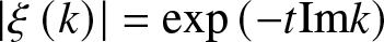 $\left\vert \xi \left(
k\right) \right\vert =\exp \left( -t\mathrm{Im}k\right) $ provides an exponential decay as
$\left\vert \xi \left(
k\right) \right\vert =\exp \left( -t\mathrm{Im}k\right) $ provides an exponential decay as  $t\rightarrow +\infty $.

Figure 1. Signature plane and deformed contour.
RHP#2 (Deformed RHP#1). Find a  $1\times2$ matrix (row) valued function $\mathbf{m}^{\left( 2\right) }\left( k\right) $ which is analytic on $\mathbb{C\diagdown}\Gamma$ and satisfies:
(1) The jump condition
 \begin{equation}
\mathbf{m}_{+}^{\left( 2\right) }\left( k\right) =\mathbf{m}_{-}^{\left(
2\right) }\left( k\right) \mathbf{V}^{\left( 2\right) }\left( k\right) \text{
for }k\in \Gamma ,
\end{equation}
\begin{equation}
\mathbf{m}_{+}^{\left( 2\right) }\left( k\right) =\mathbf{m}_{-}^{\left(
2\right) }\left( k\right) \mathbf{V}^{\left( 2\right) }\left( k\right) \text{
for }k\in \Gamma ,
\end{equation}where
 \begin{equation}
\mathbf{V}^{\left( 2\right) }(k)=
\begin{cases}
\mathbf{B}_{+}(k), & k\in \Gamma _{+} \\
\mathbf{B}_{-}(k)^{-1}, & k\in \Gamma _{-}
\end{cases}
;
\end{equation}
\begin{equation}
\mathbf{V}^{\left( 2\right) }(k)=
\begin{cases}
\mathbf{B}_{+}(k), & k\in \Gamma _{+} \\
\mathbf{B}_{-}(k)^{-1}, & k\in \Gamma _{-}
\end{cases}
;
\end{equation}(2) The symmetry condition
 \begin{equation*}
\mathbf{m}^{\left( 2\right) }\left( -k\right) =\mathbf{m}^{\left( 2\right)
}\left( k\right) \sigma_{1}\text{;}
\end{equation*}
\begin{equation*}
\mathbf{m}^{\left( 2\right) }\left( -k\right) =\mathbf{m}^{\left( 2\right)
}\left( k\right) \sigma_{1}\text{;}
\end{equation*}(3) The normalization condition
 \begin{equation*}
\mathbf{m}^{\left( 2\right) }\left( k\right) \sim \left(
\begin{array}{cc}
1 & 1
\end{array}
\right) ,k\rightarrow \infty .
\end{equation*}
\begin{equation*}
\mathbf{m}^{\left( 2\right) }\left( k\right) \sim \left(
\begin{array}{cc}
1 & 1
\end{array}
\right) ,k\rightarrow \infty .
\end{equation*}The solutions of RHP#2 and RHP#1 are related by
 \begin{equation}
\mathbf{m}^{\left( 2\right) }(k)=
\begin{cases}
\mathbf{m}^{\left( 1\right) }(k)\mathbf{B}_{+}(k)^{-1}, & k\text{is between
}\mathbb{R\ }\text{and }\Gamma _{+} \\
\mathbf{m}^{\left( 1\right) }(k)\mathbf{B}_{-}(k)^{-1}, & k\text{is between
}\mathbb{R\ }\text{and }\Gamma _{-} \\
\mathbf{m}^{\left( 1\right) }(k), & \text{elsewhere}
\end{cases}
.
\end{equation}
\begin{equation}
\mathbf{m}^{\left( 2\right) }(k)=
\begin{cases}
\mathbf{m}^{\left( 1\right) }(k)\mathbf{B}_{+}(k)^{-1}, & k\text{is between
}\mathbb{R\ }\text{and }\Gamma _{+} \\
\mathbf{m}^{\left( 1\right) }(k)\mathbf{B}_{-}(k)^{-1}, & k\text{is between
}\mathbb{R\ }\text{and }\Gamma _{-} \\
\mathbf{m}^{\left( 1\right) }(k), & \text{elsewhere}
\end{cases}
.
\end{equation} In fact, the jump along  $\mathbb{R}$ disappears but the solution between
  $
\Gamma_{-}$ and
$
\Gamma_{-}$ and  $\Gamma_{+}$ will not be needed, only outside where
 \begin{equation}
\mathbf{m}^{\left( 2\right) }(k)=\mathbf{m}^{\left( 1\right) }(k).
\end{equation}
\begin{equation}
\mathbf{m}^{\left( 2\right) }(k)=\mathbf{m}^{\left( 1\right) }(k).
\end{equation} The main feature of RHP#2 is that off-diagonal entries of  $\mathbf{V}
^{\left( 2\right) }$ along
$\mathbf{V}
^{\left( 2\right) }$ along  $\Gamma \backslash \{-1,1\}$ are exponentially decreasing as $t\rightarrow +\infty $.
7. Matrix RHP on crosses
In the previous section we have reduced our original RHP to a RHP for  $
\mathbf{m}^{\left( 2\right) }(k)$ such that away from ±1 the jumps are exponentially close to the identity as
$
\mathbf{m}^{\left( 2\right) }(k)$ such that away from ±1 the jumps are exponentially close to the identity as  $t\rightarrow +\infty $ and only parts of Γ that are close to the stationary points ±1 contribute to the solution. This prompts a new RHP, on two small crosses
  $
\Gamma _{\pm 1}=\cup _{j=1}^{4}\gamma _{\pm j}$ where
$
\Gamma _{\pm 1}=\cup _{j=1}^{4}\gamma _{\pm j}$ where  $\gamma _{\pm j}$ are given (ϵ is a small enough number which value is not essential)
 \begin{align*}
\gamma _{\pm 1}& =\{\pm 1+u\mathrm{e}^{-\mathrm{i}\pi /4},\,u\in \left[
0,\epsilon \right] \} & \gamma _{\pm 2}& =\{\pm 1+u\mathrm{e}^{\mathrm{i}\pi
/4},\,u\in \left[ 0,\epsilon \right] \} \\
\gamma _{\pm 3}& =\{\pm 1+u\mathrm{e}^{3\mathrm{i}\pi /4},\,u\in \left[
0,\epsilon \right] \} & \gamma _{\pm 4}& =\{\pm 1+u\mathrm{e}^{-3\mathrm{i}
\pi /4},\,u\in \left[ 0,\epsilon \right] \},
\end{align*}
\begin{align*}
\gamma _{\pm 1}& =\{\pm 1+u\mathrm{e}^{-\mathrm{i}\pi /4},\,u\in \left[
0,\epsilon \right] \} & \gamma _{\pm 2}& =\{\pm 1+u\mathrm{e}^{\mathrm{i}\pi
/4},\,u\in \left[ 0,\epsilon \right] \} \\
\gamma _{\pm 3}& =\{\pm 1+u\mathrm{e}^{3\mathrm{i}\pi /4},\,u\in \left[
0,\epsilon \right] \} & \gamma _{\pm 4}& =\{\pm 1+u\mathrm{e}^{-3\mathrm{i}
\pi /4},\,u\in \left[ 0,\epsilon \right] \},
\end{align*} oriented in the direction of the increase of  $\mathrm{Re}k$.
As typical in such a situation, we state our new RHP as a matrix one:
RHP#3 (Matrix RHP on small crosses). Find a  $2\times 2$ matrix valued function $\mathbf{M}^{\left( 3\right) }\left( k\right) $ which is analytic away from $\Gamma _{-1}\cup \Gamma _{+1}$ and satisfies:
(1) The jump condition
 \begin{equation*}
\mathbf{M}_{+}^{\left( 3\right) }\left( k\right) =\mathbf{M}_{-}^{\left(
3\right) }\left( k\right) \mathbf{V}^{\left( 3\right) }\left( k\right) \text{
for }k\in \Gamma _{-1}\cup \Gamma _{+1},
\end{equation*}
\begin{equation*}
\mathbf{M}_{+}^{\left( 3\right) }\left( k\right) =\mathbf{M}_{-}^{\left(
3\right) }\left( k\right) \mathbf{V}^{\left( 3\right) }\left( k\right) \text{
for }k\in \Gamma _{-1}\cup \Gamma _{+1},
\end{equation*}where
 \begin{equation*}
\mathbf{V}^{\left( 3\right) }(k)=\mathbf{V}^{\left( 2\right) }\left(
k\right) ,\ \ \ k\in \gamma _{\pm j},\ \ \ j=1,2,3,4;
\end{equation*}
\begin{equation*}
\mathbf{V}^{\left( 3\right) }(k)=\mathbf{V}^{\left( 2\right) }\left(
k\right) ,\ \ \ k\in \gamma _{\pm j},\ \ \ j=1,2,3,4;
\end{equation*}(2) The symmetry condition
 \begin{equation}
\mathbf{M}^{\left( 3\right) }\left( -k\right) =\sigma_{1}\mathbf{M}^{\left(
3\right) }\left( k\right) \sigma_{1}\text{;}
\end{equation}
\begin{equation}
\mathbf{M}^{\left( 3\right) }\left( -k\right) =\sigma_{1}\mathbf{M}^{\left(
3\right) }\left( k\right) \sigma_{1}\text{;}
\end{equation}(3) The normalization condition
 \begin{equation*}
\mathbf{M}^{\left( 3\right) }\left( k\right) \sim \mathbf{I},\ \ \
k\rightarrow \infty .
\end{equation*}
\begin{equation*}
\mathbf{M}^{\left( 3\right) }\left( k\right) \sim \mathbf{I},\ \ \
k\rightarrow \infty .
\end{equation*} Note that our enumeration of γj is chosen to agree with that of [Reference Grunert and Teschl12]. We now use the following result (see e.g. [Reference Grunert and Teschl12]). Suppose that for every sufficiently small ϵ > 0 both the L 2 and the  $
L^{\infty }$ norms of
$
L^{\infty }$ norms of  $\mathbf{V}^{\left( 2\right) }-\mathbf{I}$ are
  $
O(b\left( t\right) ^{-\beta })$ with some
$
O(b\left( t\right) ^{-\beta })$ with some  $b\left( t\right) \rightarrow
+\infty $ (given below) and β > 0 away from some ɛ neighbourhoods of the points
$b\left( t\right) \rightarrow
+\infty $ (given below) and β > 0 away from some ɛ neighbourhoods of the points  $k=\pm 1$. Moreover, suppose that the solution to the matrix problem with jump $\mathbf{V}^{\left( 2\right) }(k)$ restricted to the ϵ neighbourhood of ±1 has a solution which satisfies
 \begin{equation}
\mathbf{M}_{\pm 1}(k)=\mathbf{I}+\frac{1}{b(t)^{\alpha }}\frac{\mathbf{M}
_{\pm 1}}{k-\left( \pm 1\right) }+O(b(t)^{-\beta }),\ \ \ \left\vert
k-\left( \pm 1\right) \right\vert \gt \varepsilon
\end{equation}
\begin{equation}
\mathbf{M}_{\pm 1}(k)=\mathbf{I}+\frac{1}{b(t)^{\alpha }}\frac{\mathbf{M}
_{\pm 1}}{k-\left( \pm 1\right) }+O(b(t)^{-\beta }),\ \ \ \left\vert
k-\left( \pm 1\right) \right\vert \gt \varepsilon
\end{equation} with some  $\alpha \in \lbrack \beta /2,\beta )$. Then the solution
  $\mathbf{M
}^{\left( 3\right) }(k)$ to RHP#3 is given by
$\mathbf{M
}^{\left( 3\right) }(k)$ to RHP#3 is given by
 \begin{equation}
\mathbf{M}^{\left( 3\right) }(k)=\mathbf{I}+\frac{1}{b(t)^{\alpha }}\left(
\frac{\mathbf{M}_{1}}{k-1}+\frac{\mathbf{M}_{-1}}{k+1}\right)
+O(b(t)^{-\beta }),t\rightarrow +\infty ,
\end{equation}
\begin{equation}
\mathbf{M}^{\left( 3\right) }(k)=\mathbf{I}+\frac{1}{b(t)^{\alpha }}\left(
\frac{\mathbf{M}_{1}}{k-1}+\frac{\mathbf{M}_{-1}}{k+1}\right)
+O(b(t)^{-\beta }),t\rightarrow +\infty ,
\end{equation} where the error term depends on the distance of k to  $\gamma _{\pm
j},j=1,2,3,4$. To obey 7.1 we must have
$\gamma _{\pm
j},j=1,2,3,4$. To obey 7.1 we must have
 \begin{equation*}
\mathbf{M}_{-1}=-\sigma _{1}\mathbf{M}_{1}\sigma _{1},
\end{equation*}
\begin{equation*}
\mathbf{M}_{-1}=-\sigma _{1}\mathbf{M}_{1}\sigma _{1},
\end{equation*}and for 7.3 we finally have
 \begin{equation*}
\mathbf{M}^{\left( 3\right) }(k)\sim \mathbf{I}+\frac{1}{b(t)^{\alpha }k}
\left( \mathbf{M}_{1}-\sigma _{1}\mathbf{M}_{1}\sigma _{1}\right) ,\ \ \
k\rightarrow \infty ,t\rightarrow +\infty .
\end{equation*}
\begin{equation*}
\mathbf{M}^{\left( 3\right) }(k)\sim \mathbf{I}+\frac{1}{b(t)^{\alpha }k}
\left( \mathbf{M}_{1}-\sigma _{1}\mathbf{M}_{1}\sigma _{1}\right) ,\ \ \
k\rightarrow \infty ,t\rightarrow +\infty .
\end{equation*}Consequently the (row) solution to RHP#2 is then given by
 \begin{equation}
\mathbf{m}^{\left( 2\right) }(k)=
\begin{pmatrix}
1 & 1
\end{pmatrix}
\left\{\mathbf{I}+\frac{1}{b(t)^{\alpha }}\left( \frac{\mathbf{M}_{1}}{k-1}-
\frac{\sigma _{1}\mathbf{M}_{1}\sigma _{1}}{k+1}\right) \right\}
+O(b(t)^{-\beta }),t\rightarrow +\infty .
\end{equation}
\begin{equation}
\mathbf{m}^{\left( 2\right) }(k)=
\begin{pmatrix}
1 & 1
\end{pmatrix}
\left\{\mathbf{I}+\frac{1}{b(t)^{\alpha }}\left( \frac{\mathbf{M}_{1}}{k-1}-
\frac{\sigma _{1}\mathbf{M}_{1}\sigma _{1}}{k+1}\right) \right\}
+O(b(t)^{-\beta }),t\rightarrow +\infty .
\end{equation}Thus, the problem boils down to finding M1.
8. Asymptotics of
$\mathbf{B}_{\pm}$ around k = 1

In this section we derive necessary asymptotics of jump matrices  $\mathbf{B}
_{\pm }\left( k\right) $ at k = 1. Observing first that since k = 1 is a stationary point for the phase
$\mathbf{B}
_{\pm }\left( k\right) $ at k = 1. Observing first that since k = 1 is a stationary point for the phase  $\Phi \left( k\right) $, we have
 \begin{equation}
\xi \left( k\right) ^{2}\sim \exp \mathrm{i}\left\{-16t+24t\left(
k-1\right) ^{2}\right\} ,\ \ k\rightarrow 1.
\end{equation}
\begin{equation}
\xi \left( k\right) ^{2}\sim \exp \mathrm{i}\left\{-16t+24t\left(
k-1\right) ^{2}\right\} ,\ \ k\rightarrow 1.
\end{equation} The common substitution  $k=1+\left( 48t\right) ^{-1/2}z$ shifts our cross Γ1 to the origin and removes time dependence from the oscillatory exponential 8.1. Omitting straightforward computations based on 8.1, Theorems 3.1 and 5.1 one then gets (below
  $k=1+\left( 48t\right)
^{-1/2}z,\ \ \ z\rightarrow 0$)
$k=1+\left( 48t\right)
^{-1/2}z,\ \ \ z\rightarrow 0$)
 \begin{equation}
\begin{array}{lllll}
\textbf{B}_{-}(k)^{-1} & \sim &
\begin{pmatrix}
1 & -R_{1}\varphi \left( z\right) ^{2}\mathrm{e}^{-\mathrm{i}z^{2}/2} \\
0 & 1
\end{pmatrix}
& =:\mathbf{V}_{1}\left( z\right) , & \arg z=-\textrm{i}\pi /4 \\
\textbf{B}_{+}(k) & \sim &
\begin{pmatrix}
1 & 0 \\
R_{2}\varphi \left( z\right) ^{-2}\mathrm{e}^{\mathrm{i}z^{2}/2} & 1
\end{pmatrix}
& =:\mathbf{V}_{2}\left( z\right) , & \arg z=\textrm{i}\pi /4 \\
\textbf{B}_{+}(k) & \sim &
\begin{pmatrix}
1 & -R_{3}\varphi \left( z\right) ^{2}z^{-2}\mathrm{e}^{-\mathrm{i}z^{2}/2}
\\
0 & 1
\end{pmatrix}
& =:\mathbf{V}_{3}\left( z\right) , & \arg z=3\textrm{i}\pi /4 \\
\textbf{B}_{-}(k)^{-1} & \sim &
\begin{pmatrix}
1 & 0 \\
R_{4}\varphi \left( z\right) ^{-2}z^{-2}\mathrm{e}^{\mathrm{i}z^{2}/2} & 1
\end{pmatrix}
& =:\mathbf{V}_{4}\left( z\right) , & \arg z=-3\textrm{i}\pi /4
\end{array}
\ \ \ ,
\end{equation}
\begin{equation}
\begin{array}{lllll}
\textbf{B}_{-}(k)^{-1} & \sim &
\begin{pmatrix}
1 & -R_{1}\varphi \left( z\right) ^{2}\mathrm{e}^{-\mathrm{i}z^{2}/2} \\
0 & 1
\end{pmatrix}
& =:\mathbf{V}_{1}\left( z\right) , & \arg z=-\textrm{i}\pi /4 \\
\textbf{B}_{+}(k) & \sim &
\begin{pmatrix}
1 & 0 \\
R_{2}\varphi \left( z\right) ^{-2}\mathrm{e}^{\mathrm{i}z^{2}/2} & 1
\end{pmatrix}
& =:\mathbf{V}_{2}\left( z\right) , & \arg z=\textrm{i}\pi /4 \\
\textbf{B}_{+}(k) & \sim &
\begin{pmatrix}
1 & -R_{3}\varphi \left( z\right) ^{2}z^{-2}\mathrm{e}^{-\mathrm{i}z^{2}/2}
\\
0 & 1
\end{pmatrix}
& =:\mathbf{V}_{3}\left( z\right) , & \arg z=3\textrm{i}\pi /4 \\
\textbf{B}_{-}(k)^{-1} & \sim &
\begin{pmatrix}
1 & 0 \\
R_{4}\varphi \left( z\right) ^{-2}z^{-2}\mathrm{e}^{\mathrm{i}z^{2}/2} & 1
\end{pmatrix}
& =:\mathbf{V}_{4}\left( z\right) , & \arg z=-3\textrm{i}\pi /4
\end{array}
\ \ \ ,
\end{equation}where
 \begin{equation*}
\varphi \left( z\right) =\exp \frac{\mathrm{i}}{2\pi }\left\{\log \left(
48a^{2}t\right) \log z-\log ^{2}z\right\}
\end{equation*}
\begin{equation*}
\varphi \left( z\right) =\exp \frac{\mathrm{i}}{2\pi }\left\{\log \left(
48a^{2}t\right) \log z-\log ^{2}z\right\}
\end{equation*}and (A 0 is given by 5.7)
 \begin{equation*}
\begin{array}{cc}
R_{1}=\mathrm{e}^{16\mathrm{i}t}\dfrac{1+\mathrm{i}\kappa }{1-\mathrm{i}
\kappa }A_{0}^{2}\exp \dfrac{1}{\pi \mathrm{i}}\left\{\log a\log \left(
48t\right) +\frac{1}{4}\log ^{2}\left( 48t\right) \right\} , & R_{2}=1/R_{1}
\\
R_{3}=48a^{2}t\ R_{1}, & R_{4}=48a^{2}t/R_{1}.
\end{array}
\end{equation*}
\begin{equation*}
\begin{array}{cc}
R_{1}=\mathrm{e}^{16\mathrm{i}t}\dfrac{1+\mathrm{i}\kappa }{1-\mathrm{i}
\kappa }A_{0}^{2}\exp \dfrac{1}{\pi \mathrm{i}}\left\{\log a\log \left(
48t\right) +\frac{1}{4}\log ^{2}\left( 48t\right) \right\} , & R_{2}=1/R_{1}
\\
R_{3}=48a^{2}t\ R_{1}, & R_{4}=48a^{2}t/R_{1}.
\end{array}
\end{equation*}9. Matrix RHP on one cross
In this section we formulate (but not solve) a matrix RHP to find the constant matrix M1 in 7.4. Note also that since each ray in the small cross Γ+1 is of a fixed length ɛ, the image of Γ+1 under the change of variable  $z=\left( 48t\right) ^{1/2}\left( k-1\right) $ extends to infinity as $t\rightarrow +\infty $. This prompts introducing a new infinite cross
  $
\Gamma _{0}=\cup _{j=1}^{4}\Gamma _{j}$ where
$
\Gamma _{0}=\cup _{j=1}^{4}\Gamma _{j}$ where
 \begin{align*}
\Gamma _{1}& =\{u\mathrm{e}^{-\mathrm{i}\pi /4},\,u\in \lbrack 0,\infty )\}
& \Gamma _{2}& =\{u\mathrm{e}^{\mathrm{i}\pi /4},\,u\in \lbrack 0,\infty )\}
\\
\Gamma _{3}& =\{u\mathrm{e}^{3\mathrm{i}\pi /4},\,u\in \lbrack 0,\infty )\}
& \Gamma _{4}& =\{u\mathrm{e}^{-3\mathrm{i}\pi /4},\,u\in \lbrack 0,\infty
)\},
\end{align*}
\begin{align*}
\Gamma _{1}& =\{u\mathrm{e}^{-\mathrm{i}\pi /4},\,u\in \lbrack 0,\infty )\}
& \Gamma _{2}& =\{u\mathrm{e}^{\mathrm{i}\pi /4},\,u\in \lbrack 0,\infty )\}
\\
\Gamma _{3}& =\{u\mathrm{e}^{3\mathrm{i}\pi /4},\,u\in \lbrack 0,\infty )\}
& \Gamma _{4}& =\{u\mathrm{e}^{-3\mathrm{i}\pi /4},\,u\in \lbrack 0,\infty
)\},
\end{align*} the enumeration of  $\Gamma _{j}$ being chosen to match that of [Reference Grunert and Teschl12] for easy reference. Orient Γ0 such that the real part of z increases in the positive direction (see Figure 2).

Figure 2. Contours of one cross.
We are now ready to state our next RHP.
RHP#4 (Matrix RHP on one infinite cross). Find a  $2\times2$ matrix valued function M $^{\left( 4\right) }\left( z\right) $ which is analytic away from Γ0 and satisfies:
(1) The jump condition
 \begin{equation}
\mathbf{M}_{+}^{\left( 4\right) }\left( z\right) =\mathbf{M}_{-}^{\left(
4\right) }\left( z\right) \mathbf{V}^{\left( 4\right) }\left( z\right) \text{
for }z\in\Gamma_{0},
\end{equation}
\begin{equation}
\mathbf{M}_{+}^{\left( 4\right) }\left( z\right) =\mathbf{M}_{-}^{\left(
4\right) }\left( z\right) \mathbf{V}^{\left( 4\right) }\left( z\right) \text{
for }z\in\Gamma_{0},
\end{equation}where (Vj’s are defined by 8.2)
 \begin{equation}
\mathbf{V}^{\left( 4\right) }(z)=\mathbf{V}_{j}\left( z\right) ,z\in
\Gamma_{j},j=1,2,3,4;
\end{equation}
\begin{equation}
\mathbf{V}^{\left( 4\right) }(z)=\mathbf{V}_{j}\left( z\right) ,z\in
\Gamma_{j},j=1,2,3,4;
\end{equation}(2) The normalization condition
 \begin{equation*}
\mathbf{M}^{\left( 4\right) }\left( z\right) \sim \mathbf{I},z\rightarrow
\infty ,z\notin \Gamma _{0}.
\end{equation*}
\begin{equation*}
\mathbf{M}^{\left( 4\right) }\left( z\right) \sim \mathbf{I},z\rightarrow
\infty ,z\notin \Gamma _{0}.
\end{equation*}Note that we still use consequently numbering of our jump matrices which will be reset in the next section.
10. Rescaling and second conjugation. Model RHP
In this section we follow [Reference Grunert and Teschl12] to reduce RHP#4 to the one with the jump on the real line.
Rewrite the jump matrices Vj as follows
 \begin{align}
\mathbf{V}_{1} & =
\begin{pmatrix}
1 & -\overline{\rho}\varphi\left( z\right) ^{2}\mathrm{e}^{-\mathrm{i}
z^{2}/2} \nonumber \\
0 & 1
\end{pmatrix}
, & \mathbf{V}_{2} & =
\begin{pmatrix}
1 & 0 \nonumber \\
\rho\mathrm{e}^{\mathrm{i}z^{2}/2}/\varphi\left( z\right) ^{2} & 1
\end{pmatrix}
, \nonumber \\
\mathbf{V}_{3} & =
\begin{pmatrix}
1 & -\overline{\rho}\varphi\left( z\right) ^{2}\mathrm{e}^{-\mathrm{i}
z^{2}/2}/\left( \varepsilon z^{2}\right) \\
0 & 1
\end{pmatrix}
, & \mathbf{V}_{4} & =
\begin{pmatrix}
1 & 0 \nonumber \\
\rho\mathrm{e}^{\mathrm{i}z^{2}/2}/\left( \varepsilon\varphi\left( z\right)
^{2}z^{2}\right) & 1
\end{pmatrix}
,
\end{align}
\begin{align}
\mathbf{V}_{1} & =
\begin{pmatrix}
1 & -\overline{\rho}\varphi\left( z\right) ^{2}\mathrm{e}^{-\mathrm{i}
z^{2}/2} \nonumber \\
0 & 1
\end{pmatrix}
, & \mathbf{V}_{2} & =
\begin{pmatrix}
1 & 0 \nonumber \\
\rho\mathrm{e}^{\mathrm{i}z^{2}/2}/\varphi\left( z\right) ^{2} & 1
\end{pmatrix}
, \nonumber \\
\mathbf{V}_{3} & =
\begin{pmatrix}
1 & -\overline{\rho}\varphi\left( z\right) ^{2}\mathrm{e}^{-\mathrm{i}
z^{2}/2}/\left( \varepsilon z^{2}\right) \\
0 & 1
\end{pmatrix}
, & \mathbf{V}_{4} & =
\begin{pmatrix}
1 & 0 \nonumber \\
\rho\mathrm{e}^{\mathrm{i}z^{2}/2}/\left( \varepsilon\varphi\left( z\right)
^{2}z^{2}\right) & 1
\end{pmatrix}
,
\end{align}where
 \begin{equation*}
\rho=\mathrm{e}^{-16\mathrm{i}t}\dfrac{1-\mathrm{i}\kappa}{1+\mathrm{i}
\kappa }A_{0}^{-2}\exp\dfrac{\mathrm{i}}{\pi}\left\{\log a\log\left(
48t\right) +\frac{1}{4}\log^{2}\left( 48t\right) \right\} ,
\end{equation*}
\begin{equation*}
\rho=\mathrm{e}^{-16\mathrm{i}t}\dfrac{1-\mathrm{i}\kappa}{1+\mathrm{i}
\kappa }A_{0}^{-2}\exp\dfrac{\mathrm{i}}{\pi}\left\{\log a\log\left(
48t\right) +\frac{1}{4}\log^{2}\left( 48t\right) \right\} ,
\end{equation*}is a unimodular number,
 \begin{equation*}
\varphi\left( z\right) =\exp\frac{\mathrm{i}}{2\pi}\left\{\log\frac {1}{
\varepsilon}\log z-\log^{2}z\right\} ,
\end{equation*}
\begin{equation*}
\varphi\left( z\right) =\exp\frac{\mathrm{i}}{2\pi}\left\{\log\frac {1}{
\varepsilon}\log z-\log^{2}z\right\} ,
\end{equation*}and
 \begin{equation*}
\varepsilon=1/\left( 48a^{2}t\right)
\end{equation*}
\begin{equation*}
\varepsilon=1/\left( 48a^{2}t\right)
\end{equation*} is a small parameter as  $t\rightarrow+\infty$.
We now conjugate RHP#4 following [Reference Krüger and Teschl16] (see also [Reference Deift and Zhou8] for more details)). To this end introduce the diagonal matrix
 \begin{equation*}
\mathbf{D}=\left( \varphi\left( z\right) \mathrm{e}^{-\mathrm{i}
z^{2}/4}\right) ^{\sigma_{3}},
\end{equation*}
\begin{equation*}
\mathbf{D}=\left( \varphi\left( z\right) \mathrm{e}^{-\mathrm{i}
z^{2}/4}\right) ^{\sigma_{3}},
\end{equation*}triangular matrices
 \begin{align}
\mathbf{D}_{1} & =
\begin{pmatrix}
1 & \overline{\rho} \nonumber \\
0 & 1
\end{pmatrix}
, & \mathbf{D}_{2} & =
\begin{pmatrix}
1 & 0 \nonumber \\
\rho & 1
\end{pmatrix}
, \nonumber \\
\mathbf{D}_{3} & =
\begin{pmatrix}
1 & -\overline{\rho}/\varepsilon z^{2} \nonumber \\
0 & 1
\end{pmatrix}
, & \mathbf{D}_{4} & =
\begin{pmatrix}
1 & 0 \nonumber \\
-\rho/\varepsilon z^{2} & 1
\end{pmatrix}
\end{align}
\begin{align}
\mathbf{D}_{1} & =
\begin{pmatrix}
1 & \overline{\rho} \nonumber \\
0 & 1
\end{pmatrix}
, & \mathbf{D}_{2} & =
\begin{pmatrix}
1 & 0 \nonumber \\
\rho & 1
\end{pmatrix}
, \nonumber \\
\mathbf{D}_{3} & =
\begin{pmatrix}
1 & -\overline{\rho}/\varepsilon z^{2} \nonumber \\
0 & 1
\end{pmatrix}
, & \mathbf{D}_{4} & =
\begin{pmatrix}
1 & 0 \nonumber \\
-\rho/\varepsilon z^{2} & 1
\end{pmatrix}
\end{align}and four sectors
 \begin{align}
\Omega_{1} & =\left\{z|\arg z\in\left( -\pi/4,0\right) \right\} , &
\Omega_{2} & =\left\{z|\arg z\in\left( 0,\pi/4\right) \right\} , \nonumber \\
\Omega_{3} & =\left\{z|\arg z\in\left( 3\pi/4,\pi\right) \right\} , &
\Omega_{4} & =\left\{z|\arg z\in\left( -\pi,-3\pi/4\right) \right\} .
\end{align}
\begin{align}
\Omega_{1} & =\left\{z|\arg z\in\left( -\pi/4,0\right) \right\} , &
\Omega_{2} & =\left\{z|\arg z\in\left( 0,\pi/4\right) \right\} , \nonumber \\
\Omega_{3} & =\left\{z|\arg z\in\left( 3\pi/4,\pi\right) \right\} , &
\Omega_{4} & =\left\{z|\arg z\in\left( -\pi,-3\pi/4\right) \right\} .
\end{align}Consider the new matrix
 \begin{equation}
\mathbf{M}\left( z\right) =\mathbf{M}^{\left( 4\right) }\left( z\right)
\mathbf{D}\left( z\right) \left\{
\begin{array}{cc}
\mathbf{D}_{j}\left( z\right) , & z\in\Omega_{j} \\
\mathbf{I}, & \text{else}
\end{array}
\right. .
\end{equation}
\begin{equation}
\mathbf{M}\left( z\right) =\mathbf{M}^{\left( 4\right) }\left( z\right)
\mathbf{D}\left( z\right) \left\{
\begin{array}{cc}
\mathbf{D}_{j}\left( z\right) , & z\in\Omega_{j} \\
\mathbf{I}, & \text{else}
\end{array}
\right. .
\end{equation} Arguing along the same lines as [Reference Krüger and Teschl16] (see also [Reference Deift and Zhou8] for more detail) one can show that the substitution 10.4 removes the jumps across all  $\Gamma_{j}$ but introduces a jump across the real line instead. Indeed, since
  $\mathbf{M}^{\left( 4\right)
}\left( z\right) $ has no jump across the real line we have
$\mathbf{M}^{\left( 4\right)
}\left( z\right) $ has no jump across the real line we have
 \begin{equation*}
\mathbf{M}_{+}\left( z\right) =\mathbf{M}^{\left( 4\right) }\left( z\right)
\left\{
\begin{array}{cc}
\mathbf{D}_{+}\left( z\right) \mathbf{D}_{3}\left( z\right) , & z \lt 0 \nonumber \\
\mathbf{D}_{+}\left( z\right) \mathbf{D}_{2}, & z \gt 0
\end{array}
\right. ,
\end{equation*}
\begin{equation*}
\mathbf{M}_{+}\left( z\right) =\mathbf{M}^{\left( 4\right) }\left( z\right)
\left\{
\begin{array}{cc}
\mathbf{D}_{+}\left( z\right) \mathbf{D}_{3}\left( z\right) , & z \lt 0 \nonumber \\
\mathbf{D}_{+}\left( z\right) \mathbf{D}_{2}, & z \gt 0
\end{array}
\right. ,
\end{equation*} \begin{equation*}
\mathbf{M}_{-}\left( z\right) =\mathbf{M}^{\left( 4\right) }\left( z\right)
\left\{
\begin{array}{cc}
\mathbf{D}_{-}\left( z\right) \mathbf{D}_{4}\left( z\right) , & z \lt 0 \nonumber \\
\mathbf{D}_{-}\left( z\right) \mathbf{D}_{1}, & z \gt 0
\end{array}
\right. ,
\end{equation*}
\begin{equation*}
\mathbf{M}_{-}\left( z\right) =\mathbf{M}^{\left( 4\right) }\left( z\right)
\left\{
\begin{array}{cc}
\mathbf{D}_{-}\left( z\right) \mathbf{D}_{4}\left( z\right) , & z \lt 0 \nonumber \\
\mathbf{D}_{-}\left( z\right) \mathbf{D}_{1}, & z \gt 0
\end{array}
\right. ,
\end{equation*}and therefore
 \begin{equation*}
\mathbf{M}_{+}\left( z\right) =\mathbf{M}_{-}\left( z\right) \left\{
\begin{array}{cc}
\mathbf{D}_{4}\left( z\right) ^{-1}\mathbf{D}_{-}\left( z\right) ^{-1}
\mathbf{D}_{+}\left( z\right) \mathbf{D}_{3}\left( z\right) , & z \lt 0 \\
\mathbf{D}_{1}{}^{-1}\mathbf{D}_{-}\left( z\right) ^{-1}\mathbf{D}_{+}\left(
z\right) \mathbf{D}_{2}, & z \gt 0
\end{array}
\right. .
\end{equation*}
\begin{equation*}
\mathbf{M}_{+}\left( z\right) =\mathbf{M}_{-}\left( z\right) \left\{
\begin{array}{cc}
\mathbf{D}_{4}\left( z\right) ^{-1}\mathbf{D}_{-}\left( z\right) ^{-1}
\mathbf{D}_{+}\left( z\right) \mathbf{D}_{3}\left( z\right) , & z \lt 0 \\
\mathbf{D}_{1}{}^{-1}\mathbf{D}_{-}\left( z\right) ^{-1}\mathbf{D}_{+}\left(
z\right) \mathbf{D}_{2}, & z \gt 0
\end{array}
\right. .
\end{equation*}By a direct computation one shows
 \begin{equation*}
\mathbf{D}_{+}\left( z\right) =\mathbf{D}_{-}\left( z\right) \left\{
\begin{array}{cc}
\left( \varepsilon z^{2}\right) ^{\sigma_{3}}, & z \lt 0 \\
\mathbf{I}, & z \gt 0
\end{array}
\right. ,
\end{equation*}
\begin{equation*}
\mathbf{D}_{+}\left( z\right) =\mathbf{D}_{-}\left( z\right) \left\{
\begin{array}{cc}
\left( \varepsilon z^{2}\right) ^{\sigma_{3}}, & z \lt 0 \\
\mathbf{I}, & z \gt 0
\end{array}
\right. ,
\end{equation*}and for the jump matrix we explicitly have
 \begin{equation*}
\mathbf{J}\left( z\right) :=\left(
\begin{array}{cc}
\varepsilon z^{2} & -\overline{\rho} \\
\rho & 0
\end{array}
\right) ,z \lt 0
\end{equation*}
\begin{equation*}
\mathbf{J}\left( z\right) :=\left(
\begin{array}{cc}
\varepsilon z^{2} & -\overline{\rho} \\
\rho & 0
\end{array}
\right) ,z \lt 0
\end{equation*} \begin{equation*}
\mathbf{J}\left( z\right) :=\left(
\begin{array}{cc}
0 & -\overline{\rho} \\
\rho & 1
\end{array}
\right) ,z \gt 0.
\end{equation*}
\begin{equation*}
\mathbf{J}\left( z\right) :=\left(
\begin{array}{cc}
0 & -\overline{\rho} \\
\rho & 1
\end{array}
\right) ,z \gt 0.
\end{equation*}This leads to a new RHP:
RHP#5 (Model RHP). Find a  $2\times2$ matrix valued function M $\left( z\right) $ which is analytic on $\mathbb{C\diagdown R}$ and satisfies:
(1) The jump condition
 \begin{equation}
\mathbf{M}_{+}\left( z\right) =\mathbf{M}_{-}\left( z\right) \mathbf{J}
\left( z\right) \text{for }z\in\mathbb{R},
\end{equation}
\begin{equation}
\mathbf{M}_{+}\left( z\right) =\mathbf{M}_{-}\left( z\right) \mathbf{J}
\left( z\right) \text{for }z\in\mathbb{R},
\end{equation}where
 \begin{equation}
\mathbf{J}(z)=\left(
\begin{array}{cc}
\varepsilon z^{2}\mathrm{1}_{\left( -\infty,0\right) } & -\overline{\rho} \\
\rho & \mathrm{1}_{\left( 0,\infty\right) }
\end{array}
\right) ,z\in\mathbb{R};
\end{equation}
\begin{equation}
\mathbf{J}(z)=\left(
\begin{array}{cc}
\varepsilon z^{2}\mathrm{1}_{\left( -\infty,0\right) } & -\overline{\rho} \\
\rho & \mathrm{1}_{\left( 0,\infty\right) }
\end{array}
\right) ,z\in\mathbb{R};
\end{equation}(2) The normalization condition
 \begin{equation}
\mathbf{M}\left( z\right) \sim \left( \varphi \left( z\right) \mathrm{e}^{-
\mathrm{i}z^{2}/4}\right) ^{\sigma _{3}},z\rightarrow \infty ,\arg z\in
\left( \pi /4,3\pi /4\right) .
\end{equation}
\begin{equation}
\mathbf{M}\left( z\right) \sim \left( \varphi \left( z\right) \mathrm{e}^{-
\mathrm{i}z^{2}/4}\right) ^{\sigma _{3}},z\rightarrow \infty ,\arg z\in
\left( \pi /4,3\pi /4\right) .
\end{equation}Just, we are back to the original contour, the real line, but as apposed to RHP#0 it is a matrix one now. The relation between RHP#4 and RHP#5 is again given by 10.4.
Recall that in the classical case (i.e. under condition 1.3)  $\left\vert R\left( \pm1\right) \right\vert \lt 1$, which leads to a constant jump matrix, whereas in our case it is not. A similar situation was recently considered in [Reference Budylin5] where the first diagonal entry of 10.6 vanishes at z = 0 linearly. It was shown in [Reference Budylin5] that the corresponding RHP can in a certain sense be considered as a perturbation of the model RHP with a constant jump matrix. This idea works in our situation too.
11. Additive RHP
In this section we solve RHP#5 by transforming it to an additive RHP that is already solved in [Reference Budylin5]. For the reader’s convenience we sketch some steps. Following [Reference Krüger and Teschl16] (see also [Reference Budylin5], [Reference Deift and Zhou8]), introduce a new matrix
 \begin{equation}
\mathbf{N}\left( z\right) :=\left( \frac{\mathrm{d}\mathbf{M}}{\mathrm{d}z}
\right) \mathbf{M}^{-1}+\frac{\mathrm{i}z}{2}\sigma _{3},
\end{equation}
\begin{equation}
\mathbf{N}\left( z\right) :=\left( \frac{\mathrm{d}\mathbf{M}}{\mathrm{d}z}
\right) \mathbf{M}^{-1}+\frac{\mathrm{i}z}{2}\sigma _{3},
\end{equation} where M is given by 10.4. The matrix N is clearly analytic away from  $(-\infty ,0]$ and has a jump across $(-\infty ,0]$. Omitting straightforward computations, one has an additive RHP:
 \begin{align}
& \mathbf{N}_{+}\left( z\right) -\mathbf{N}_{-}\left( z\right)\nonumber \\
& =\frac{2}{z}\mathbf{M}^{\left( 4\right) }\left(
\begin{array}{cc}
1 & -\overline{\rho }\varphi \left( -z\right) ^{2}\mathrm{e}^{-\mathrm{i}
z^{2}/2} \nonumber \\
\rho \varphi \left( -z\right) ^{-2}\mathrm{e}^{\mathrm{i}z^{2}/2} & -1
\end{array}
\right) \left( \mathbf{M}^{\left( 4\right) }\right) ^{-1}\mathrm{1}_{\left(
-\infty ,0\right) } \nonumber \\
& :=\mathbf{E}\left( z\right) ,\ \ \ z\in \mathbb{R},
\end{align}
\begin{align}
& \mathbf{N}_{+}\left( z\right) -\mathbf{N}_{-}\left( z\right)\nonumber \\
& =\frac{2}{z}\mathbf{M}^{\left( 4\right) }\left(
\begin{array}{cc}
1 & -\overline{\rho }\varphi \left( -z\right) ^{2}\mathrm{e}^{-\mathrm{i}
z^{2}/2} \nonumber \\
\rho \varphi \left( -z\right) ^{-2}\mathrm{e}^{\mathrm{i}z^{2}/2} & -1
\end{array}
\right) \left( \mathbf{M}^{\left( 4\right) }\right) ^{-1}\mathrm{1}_{\left(
-\infty ,0\right) } \nonumber \\
& :=\mathbf{E}\left( z\right) ,\ \ \ z\in \mathbb{R},
\end{align} for N which is considered in [Reference Budylin5] (only some coefficients are different). We have a less technical approach to 11.2 (it will be given elsewhere) but here we follow [Reference Budylin5]. Introducing an error  $O\left( \varepsilon ^{1/2}\log
\varepsilon \right) $ we replace 11.2 with
$O\left( \varepsilon ^{1/2}\log
\varepsilon \right) $ we replace 11.2 with
 \begin{equation}
\mathcal{N}_{+}\left( z\right) -\mathcal{N}_{-}\left( z\right) =\mathcal{E}
\left( z\right) ,
\end{equation}
\begin{equation}
\mathcal{N}_{+}\left( z\right) -\mathcal{N}_{-}\left( z\right) =\mathcal{E}
\left( z\right) ,
\end{equation}where
 \begin{align}
\mathcal{E}\left( z\right) & =\frac{2}{z}\left(
\begin{array}{cc}
1 & -\overline{\rho }\varphi \left( -z\right) ^{2}\mathrm{e}^{-\mathrm{i}
z^{2}/2} \\
\rho \varphi \left( -z\right) ^{-2}\mathrm{e}^{\mathrm{i}z^{2}/2} & -1
\end{array}
\right) \mathrm{1}_{\left( -\infty ,0\right) } \nonumber\\
& =\frac{2}{z}\mathrm{1}_{\left( -\infty ,0\right) }\sigma _{3}+\frac{2}{z}
\left(
\begin{array}{cc}
0 & -\overline{\rho }\varphi \left( -z\right) ^{2}\mathrm{e}^{-\mathrm{i}
z^{2}/2} \\
\rho \varphi \left( -z\right) ^{-2}\mathrm{e}^{\mathrm{i}z^{2}/2} & 0
\end{array}
\right) \mathrm{1}_{\left( -\infty ,0\right) }.
\end{align}
\begin{align}
\mathcal{E}\left( z\right) & =\frac{2}{z}\left(
\begin{array}{cc}
1 & -\overline{\rho }\varphi \left( -z\right) ^{2}\mathrm{e}^{-\mathrm{i}
z^{2}/2} \\
\rho \varphi \left( -z\right) ^{-2}\mathrm{e}^{\mathrm{i}z^{2}/2} & -1
\end{array}
\right) \mathrm{1}_{\left( -\infty ,0\right) } \nonumber\\
& =\frac{2}{z}\mathrm{1}_{\left( -\infty ,0\right) }\sigma _{3}+\frac{2}{z}
\left(
\begin{array}{cc}
0 & -\overline{\rho }\varphi \left( -z\right) ^{2}\mathrm{e}^{-\mathrm{i}
z^{2}/2} \\
\rho \varphi \left( -z\right) ^{-2}\mathrm{e}^{\mathrm{i}z^{2}/2} & 0
\end{array}
\right) \mathrm{1}_{\left( -\infty ,0\right) }.
\end{align} We then split  $\mathcal{E=E}_{+}-\mathcal{E}_{-}$ where $\mathcal{E}_{\pm }$ and functions that can be analytically continued into $\mathbb{C}^{\pm }$ as follows (recalling our notation $z_{\pm }=z\pm \mathrm{i}0$)
 \begin{align}
\mathcal{E}_{\pm }\left( z\right) & = -\frac{\mathrm{i}}{\pi }\frac{\log
z_{\pm }}{z}\sigma _{3} \nonumber\\
& -\frac{\mathrm{i}}{z}\frac{1}{\pi }\int_{-\infty }^{0}\frac{z+\mathrm{i}}{
s-z_{\pm }}\left(
\begin{array}{cc}
0 & -\overline{\rho }\varphi \left( -s\right) ^{2}\mathrm{e}^{-\mathrm{i}
s^{2}/2} \\
\rho \varphi \left( -s\right) ^{-2}\mathrm{e}^{\mathrm{i}s^{2}/2} & 0
\end{array}
\right) \frac{\mathrm{d}s}{s+\mathrm{i}}.
\end{align}
\begin{align}
\mathcal{E}_{\pm }\left( z\right) & = -\frac{\mathrm{i}}{\pi }\frac{\log
z_{\pm }}{z}\sigma _{3} \nonumber\\
& -\frac{\mathrm{i}}{z}\frac{1}{\pi }\int_{-\infty }^{0}\frac{z+\mathrm{i}}{
s-z_{\pm }}\left(
\begin{array}{cc}
0 & -\overline{\rho }\varphi \left( -s\right) ^{2}\mathrm{e}^{-\mathrm{i}
s^{2}/2} \\
\rho \varphi \left( -s\right) ^{-2}\mathrm{e}^{\mathrm{i}s^{2}/2} & 0
\end{array}
\right) \frac{\mathrm{d}s}{s+\mathrm{i}}.
\end{align} Substituting 11.5 in 11.3 leads to the conclusion that the function  $N_{+}\left( z\right) -\mathcal{E
}_{+}\left( z\right) $ is analytic on
$N_{+}\left( z\right) -\mathcal{E
}_{+}\left( z\right) $ is analytic on  $\mathbb{C}$ except for z = 0 where it may have a simple pole (this is due to discontinuity of
  $\mathbf{J}\left(
z\right) $ at z = 0). That is, the matrix function
$\mathbf{J}\left(
z\right) $ at z = 0). That is, the matrix function
 \begin{align*}
& \left( \frac{\mathrm{d}\mathbf{M}}{\mathrm{d}z}\right) \mathbf{M}^{-1}+
\frac{\mathrm{i}z}{2}\sigma _{3}+\frac{\mathrm{i}}{\pi }\frac{\log z}{z}
\sigma _{3} \\
& +\frac{\mathrm{i}}{z}\int_{0}^{\infty }\frac{z+\mathrm{i}}{s+z}\frac{
\mathbf{F}\left( s\right) }{s-\mathrm{i}}\frac{\mathrm{d}s}{\pi }+\frac{
\mathbf{A}}{z},
\end{align*}
\begin{align*}
& \left( \frac{\mathrm{d}\mathbf{M}}{\mathrm{d}z}\right) \mathbf{M}^{-1}+
\frac{\mathrm{i}z}{2}\sigma _{3}+\frac{\mathrm{i}}{\pi }\frac{\log z}{z}
\sigma _{3} \\
& +\frac{\mathrm{i}}{z}\int_{0}^{\infty }\frac{z+\mathrm{i}}{s+z}\frac{
\mathbf{F}\left( s\right) }{s-\mathrm{i}}\frac{\mathrm{d}s}{\pi }+\frac{
\mathbf{A}}{z},
\end{align*}where
 \begin{equation*}
\mathbf{F}\left( s\right) :=\left(
\begin{array}{cc}
0 & -\overline{\rho }f\left( s\right) \\
\rho \overline{f\left( s\right) } & 0
\end{array}
\right) ,f\left( s\right) :=\varphi \left( s\right) ^{2}\mathrm{e}^{-\mathrm{
i}s^{2}/2}
\end{equation*}
\begin{equation*}
\mathbf{F}\left( s\right) :=\left(
\begin{array}{cc}
0 & -\overline{\rho }f\left( s\right) \\
\rho \overline{f\left( s\right) } & 0
\end{array}
\right) ,f\left( s\right) :=\varphi \left( s\right) ^{2}\mathrm{e}^{-\mathrm{
i}s^{2}/2}
\end{equation*}is entire for some constant matrix A. As in the classical case, this leads to a first order matrix differential equation. The latter can be rewritten as a system of second order ODEs that are perturbations of Bessel equations. As opposed to the classical case we cannot solve them explicitly but can asymptotically, which leads to
 \begin{align}
\mathbf{M}\left( z\right) & \sim \left( \mathbf{I}+\dfrac{\mathrm{i}}{z}
\left(
\begin{array}{cc}
0 & -\beta \nonumber \\
\overline{\beta } & 0
\end{array}
\right) \right) \left( \varphi \left( z\right) \mathrm{e}^{-\mathrm{i}
z^{2}/4}\right) ^{\sigma _{3}},\nonumber \\
z& \rightarrow \infty ,\ \ \ \arg z\in \left( \pi /4,3\pi /4\right) ,\ \ \
t\rightarrow +\infty ,
\end{align}
\begin{align}
\mathbf{M}\left( z\right) & \sim \left( \mathbf{I}+\dfrac{\mathrm{i}}{z}
\left(
\begin{array}{cc}
0 & -\beta \nonumber \\
\overline{\beta } & 0
\end{array}
\right) \right) \left( \varphi \left( z\right) \mathrm{e}^{-\mathrm{i}
z^{2}/4}\right) ^{\sigma _{3}},\nonumber \\
z& \rightarrow \infty ,\ \ \ \arg z\in \left( \pi /4,3\pi /4\right) ,\ \ \
t\rightarrow +\infty ,
\end{align}where
 \begin{equation}
\beta =\sqrt{\nu }\overline{\rho }\exp \mathrm{i}\left\{\pi /4+\arg \Gamma
\left( \mathrm{i}\nu \right) \right\} .
\end{equation}
\begin{equation}
\beta =\sqrt{\nu }\overline{\rho }\exp \mathrm{i}\left\{\pi /4+\arg \Gamma
\left( \mathrm{i}\nu \right) \right\} .
\end{equation} Here Γ is the Euler gamma function,  $\nu =\nu \left( \varepsilon
\right) =-\left( 1/2\pi \right) \log \varepsilon $, and
$\nu =\nu \left( \varepsilon
\right) =-\left( 1/2\pi \right) \log \varepsilon $, and  $\varphi \left(
z\right) $ is given by
$\varphi \left(
z\right) $ is given by
 \begin{equation*}
\varphi \left( z\right) =\exp \left\{\mathrm{i}\nu \left( \varepsilon
\right) \log z+\frac{1}{2\pi \mathrm{i}}\log ^{2}z\right\} \text{.}
\end{equation*}
\begin{equation*}
\varphi \left( z\right) =\exp \left\{\mathrm{i}\nu \left( \varepsilon
\right) \log z+\frac{1}{2\pi \mathrm{i}}\log ^{2}z\right\} \text{.}
\end{equation*}12. Proof of the main theorem
With all our preparation in order, to proof Theorem 3.3 we merely need to do a chain of back substitutions to 4.5. The end product is available in [Reference Grunert and Teschl12]:
 \begin{equation*}
\left. q\left( x,t\right) \right\vert _{x=-12t}\sim \sqrt{\frac{4}{3t}}\mathrm{Im}\beta \left( t\right) ,\ \ \ t\rightarrow +\infty ,
\end{equation*}
\begin{equation*}
\left. q\left( x,t\right) \right\vert _{x=-12t}\sim \sqrt{\frac{4}{3t}}\mathrm{Im}\beta \left( t\right) ,\ \ \ t\rightarrow +\infty ,
\end{equation*}where β is given by 11.7:
 \begin{align*}
\beta \left( t\right) & =\sqrt{\nu \left( t\right) }\overline{\rho }\left(
t\right) \exp \mathrm{i}\left\{\frac{\pi }{4}+\arg \Gamma \left( \mathrm{i}
\nu \left( t\right) \right) \right\} \\
& \sim \sqrt{\nu \left( t\right) }\overline{\rho }\left( t\right) \exp
\mathrm{i}\left( \nu \left( t\right) \log \nu \left( t\right) -\nu \left(
t\right) \right) ,t\rightarrow +\infty .
\end{align*}
\begin{align*}
\beta \left( t\right) & =\sqrt{\nu \left( t\right) }\overline{\rho }\left(
t\right) \exp \mathrm{i}\left\{\frac{\pi }{4}+\arg \Gamma \left( \mathrm{i}
\nu \left( t\right) \right) \right\} \\
& \sim \sqrt{\nu \left( t\right) }\overline{\rho }\left( t\right) \exp
\mathrm{i}\left( \nu \left( t\right) \log \nu \left( t\right) -\nu \left(
t\right) \right) ,t\rightarrow +\infty .
\end{align*} Here  $\nu \left( t\right) =\left( 1/2\pi \right) \log \left( 48a^{2}t\right)
$ and we have used the well-known asymptotic
$\nu \left( t\right) =\left( 1/2\pi \right) \log \left( 48a^{2}t\right)
$ and we have used the well-known asymptotic
 \begin{equation*}
\arg \Gamma \left( \mathrm{i}y\right) \sim y\log y-y-\pi /4,\ \ \
y\rightarrow +\infty .
\end{equation*}
\begin{equation*}
\arg \Gamma \left( \mathrm{i}y\right) \sim y\log y-y-\pi /4,\ \ \
y\rightarrow +\infty .
\end{equation*}Since
 \begin{equation*}
\overline{\rho }=\mathrm{e}^{16\mathrm{i}t}\dfrac{1+\mathrm{i}\kappa }{1-
\mathrm{i}\kappa }A_{0}^{2}\exp \dfrac{1}{\mathrm{i}\pi }\left\{\log a\log
\left( 48t\right) +\frac{1}{4}\log ^{2}\left( 48t\right) \right\} ,
\end{equation*}
\begin{equation*}
\overline{\rho }=\mathrm{e}^{16\mathrm{i}t}\dfrac{1+\mathrm{i}\kappa }{1-
\mathrm{i}\kappa }A_{0}^{2}\exp \dfrac{1}{\mathrm{i}\pi }\left\{\log a\log
\left( 48t\right) +\frac{1}{4}\log ^{2}\left( 48t\right) \right\} ,
\end{equation*}where A 0 is given by 5.7, it follows from 11.7 that
 \begin{align*}
\left. q\left( x,t\right) \right\vert _{x=-12t}& \sim 2\left( 3t\right)
^{-1/2}\mathrm{Im}\beta \left( t\right) \\
& =\sqrt{\frac{4\nu \left( t\right) }{3t}}\mathrm{Im}\left\{\overline{\rho
\left( t\right) }\exp \mathrm{i}\left[ \nu \left( t\right) \log \nu \left(
t\right) -\nu \left( t\right) \right] \right\} \\
& =\sqrt{\frac{4\nu \left( t\right) }{3t}}\sin \left\{16t-\nu \left(
t\right) \left[ 1+\pi \nu \left( t\right) -\log \nu \left( t\right) \right]
+\delta \right\} ,
\end{align*}
\begin{align*}
\left. q\left( x,t\right) \right\vert _{x=-12t}& \sim 2\left( 3t\right)
^{-1/2}\mathrm{Im}\beta \left( t\right) \\
& =\sqrt{\frac{4\nu \left( t\right) }{3t}}\mathrm{Im}\left\{\overline{\rho
\left( t\right) }\exp \mathrm{i}\left[ \nu \left( t\right) \log \nu \left(
t\right) -\nu \left( t\right) \right] \right\} \\
& =\sqrt{\frac{4\nu \left( t\right) }{3t}}\sin \left\{16t-\nu \left(
t\right) \left[ 1+\pi \nu \left( t\right) -\log \nu \left( t\right) \right]
+\delta \right\} ,
\end{align*}where
 \begin{align*}
\delta & =\frac{2}{\pi }\int\limits_{0}^{1}\log \left\vert \frac{
T(s)/T^{\prime }\left( 1\right) }{1-s}\right\vert ^{2}\frac{ds}{1-s^{2}}-
\frac{2}{\pi }\int\limits_{0}^{1}\frac{\log s{\mathrm{d}s}}{s-2} \\
& +\frac{1}{\pi }\log \frac{\kappa ^{3}+\kappa }{2}\log \frac{\kappa
^{3}+\kappa }{8}-\frac{\pi }{3}+\arctan \frac{2\kappa }{1-\kappa ^{2}}.
\end{align*}
\begin{align*}
\delta & =\frac{2}{\pi }\int\limits_{0}^{1}\log \left\vert \frac{
T(s)/T^{\prime }\left( 1\right) }{1-s}\right\vert ^{2}\frac{ds}{1-s^{2}}-
\frac{2}{\pi }\int\limits_{0}^{1}\frac{\log s{\mathrm{d}s}}{s-2} \\
& +\frac{1}{\pi }\log \frac{\kappa ^{3}+\kappa }{2}\log \frac{\kappa
^{3}+\kappa }{8}-\frac{\pi }{3}+\arctan \frac{2\kappa }{1-\kappa ^{2}}.
\end{align*}Thus, the theorem is proven.
13. Concluding remarks
In this final section we make some remarks on what we have not done.
1. We state our main result for just one ray,  $x=-12t$, and not for a wider region as it is typically done. The main reason is that otherwise we would not be able to rely directly on [Reference Budylin5]. We fill in this gap elsewhere by offering an independent of [Reference Budylin5] approach.
2. We believe that Theorem 3.3 holds for initial data of the form 3.6 but supported on  $\left( 0,\infty
\right) $. However, RHP#0 for this case is no longer regular since
$\left( 0,\infty
\right) $. However, RHP#0 for this case is no longer regular since  $
m^{\left( +\right) }(k,x)$ has now a simple pole at ±1 which means that
$
m^{\left( +\right) }(k,x)$ has now a simple pole at ±1 which means that  $\mathbf{m}(k,x,t)$ has a first order singularity and thus RHP#0 is singular. However this issue does not arise if in place of (1.7) we use the left scattering identity
 \begin{equation}
T(k)\psi ^{\left( +\right) }(x,k)=\overline{\psi ^{\left( -\right) }(x,k)}
+L(k)\psi ^{\left( -\right) }(x,k),\text{k}\in \mathbb{R},
\end{equation}
\begin{equation}
T(k)\psi ^{\left( +\right) }(x,k)=\overline{\psi ^{\left( -\right) }(x,k)}
+L(k)\psi ^{\left( -\right) }(x,k),\text{k}\in \mathbb{R},
\end{equation}where T is the same as above and L is the left reflection coefficient. But we know that L = R in our case. As before 13.1 leads to a new row vector
 \begin{equation}
\mathbf{m}(k,x,t)=\left\{
\begin{array}{c@{\quad}l}
\begin{pmatrix}
T(k)m^{\left( +\right) }(k,x,t) & m^{\left( -\right) }(k,x,t)
\end{pmatrix}
, & \mathrm{Im}k \gt 0, \\
\begin{pmatrix}
m^{\left( -\right) }(-k,x,t) & T(-k)m^{\left( +\right) }(-k,x,t)
\end{pmatrix}
, & \mathrm{Im}k \lt 0,
\end{array}
\right.
\end{equation}
\begin{equation}
\mathbf{m}(k,x,t)=\left\{
\begin{array}{c@{\quad}l}
\begin{pmatrix}
T(k)m^{\left( +\right) }(k,x,t) & m^{\left( -\right) }(k,x,t)
\end{pmatrix}
, & \mathrm{Im}k \gt 0, \\
\begin{pmatrix}
m^{\left( -\right) }(-k,x,t) & T(-k)m^{\left( +\right) }(-k,x,t)
\end{pmatrix}
, & \mathrm{Im}k \lt 0,
\end{array}
\right.
\end{equation} where, as before,  $m^{\left( \pm \right) }(k;x,t)=$e
  $^{\mp
\mathrm{i}kx}\psi ^{\left( \pm \right) }(x,t;k)$, which satisfies the jump condition
$^{\mp
\mathrm{i}kx}\psi ^{\left( \pm \right) }(x,t;k)$, which satisfies the jump condition
 \begin{equation}
\mathbf{m}_{+}\left( k\right) =\mathbf{m}_{-}\left( k\right) \mathbf{V}
\left( k\right) \text{for }k\in \mathbb{R},
\end{equation}
\begin{equation}
\mathbf{m}_{+}\left( k\right) =\mathbf{m}_{-}\left( k\right) \mathbf{V}
\left( k\right) \text{for }k\in \mathbb{R},
\end{equation}where
 \begin{equation}
\mathbf{V}\left( k\right) =\left(
\begin{array}{cc}
1-\left\vert R\left( k\right) \right\vert ^{2} & -\overline{R}\left(
k\right) \xi \left( k\right) ^{2} \\
R\left( k\right) \xi \left( k\right) ^{-2} & 1
\end{array}
\right) .
\end{equation}
\begin{equation}
\mathbf{V}\left( k\right) =\left(
\begin{array}{cc}
1-\left\vert R\left( k\right) \right\vert ^{2} & -\overline{R}\left(
k\right) \xi \left( k\right) ^{2} \\
R\left( k\right) \xi \left( k\right) ^{-2} & 1
\end{array}
\right) .
\end{equation} Note that the only difference between 13.4 and 4.4 is the sign of the power of  $\xi
\left( k\right) $ which is the opposite. The well-posedness of the new RHP is a more complicated question but it does hold. The next difference is of course the signature diagram (Figure 1) where all signs change to the opposite which leads to a different conjugation step. Instead of T 0 we conjugate our RHP with
$\xi
\left( k\right) $ which is the opposite. The well-posedness of the new RHP is a more complicated question but it does hold. The next difference is of course the signature diagram (Figure 1) where all signs change to the opposite which leads to a different conjugation step. Instead of T 0 we conjugate our RHP with  $T/T_{0}$ and in place of 6.3 and 6.4 we have
 \begin{equation*}
\mathbf{B}_{-}(k)=\left\{
\begin{array}{ccc}
\begin{pmatrix}
1 & 0 \\
-\dfrac{R(k)T_{0-}(k)^{2}\xi\left( k\right) ^{-2}}{T\left( k\right)
^{2}T\left( k\right) T\left( -k\right) } & 1
\end{pmatrix}
& , & k\in\mathbb{R}\backslash\left[ -1,1\right] \\
\begin{pmatrix}
1 & \dfrac{R(-k)T\left( k\right) ^{2}}{T_{0}\left( k\right) ^{2}\xi\left(
k\right) ^{-2}} \\
0 & 1
\end{pmatrix}
& , & k\in\left[ -1,1\right]
\end{array}
\right. ,
\end{equation*}
\begin{equation*}
\mathbf{B}_{-}(k)=\left\{
\begin{array}{ccc}
\begin{pmatrix}
1 & 0 \\
-\dfrac{R(k)T_{0-}(k)^{2}\xi\left( k\right) ^{-2}}{T\left( k\right)
^{2}T\left( k\right) T\left( -k\right) } & 1
\end{pmatrix}
& , & k\in\mathbb{R}\backslash\left[ -1,1\right] \\
\begin{pmatrix}
1 & \dfrac{R(-k)T\left( k\right) ^{2}}{T_{0}\left( k\right) ^{2}\xi\left(
k\right) ^{-2}} \\
0 & 1
\end{pmatrix}
& , & k\in\left[ -1,1\right]
\end{array}
\right. ,
\end{equation*} \begin{equation*}
\mathbf{B}_{+}(k)=\left\{
\begin{array}{ccc}
\begin{pmatrix}
1 & -\dfrac{T\left( k\right) ^{2}R(-k)\xi\left( k\right) ^{2}}{T_{0+}\left(
k\right) ^{2}T\left( k\right) T\left( -k\right) } \\
0 & 1
\end{pmatrix}
& , & k\in\mathbb{R}\backslash\left[ -1,1\right] \\
\begin{pmatrix}
1 & 0 \\
\dfrac{R(k)T_{0}\left( k\right) ^{2}\xi\left( k\right) ^{-2}}{T\left(
k\right) ^{2}} & 1
\end{pmatrix}
& , & k\in\left[ -1,1\right]
\end{array}
\right. .
\end{equation*}
\begin{equation*}
\mathbf{B}_{+}(k)=\left\{
\begin{array}{ccc}
\begin{pmatrix}
1 & -\dfrac{T\left( k\right) ^{2}R(-k)\xi\left( k\right) ^{2}}{T_{0+}\left(
k\right) ^{2}T\left( k\right) T\left( -k\right) } \\
0 & 1
\end{pmatrix}
& , & k\in\mathbb{R}\backslash\left[ -1,1\right] \\
\begin{pmatrix}
1 & 0 \\
\dfrac{R(k)T_{0}\left( k\right) ^{2}\xi\left( k\right) ^{-2}}{T\left(
k\right) ^{2}} & 1
\end{pmatrix}
& , & k\in\left[ -1,1\right]
\end{array}
\right. .
\end{equation*}Continuing the same way as we did above, we get to a model RHP with a more complicated jump matrix. We plan to come back to it elsewhere.
γ) hinges on understanding the zero energy behaviour of scattering data. Note that this problem was first explicitly mentioned in [Reference Klaus14]. The paper [Reference Yafaev26] suggests that this is a very difficult problem in general. We should emphasize in this connection that as opposed to the short-range scattering theory, its WvN type counterpart is not understood to the level suitable to do the IST. It is to say that there is no “one stop shopping” like [Reference Deift and Trubowitz6] or [Reference Marchenko and Iacob17] available for facts related to long-range direct/inverse scattering.
Acknowledgements
The author acknowledges partial support from NSF under grant DMS-2307774. We are also thankful to Deniz Bilman for stimulating discussions and the referees for valuable comments.
Funding statement
The author is supported in part by the NSF under grant DMS-2307774.

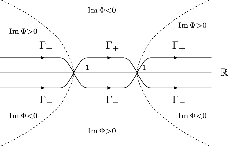
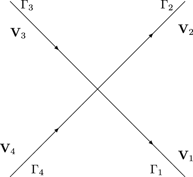

 Open access