The Aftermath of Sovereign Debt Crises: A Narrative Approach

Abstract

This paper investigates the causal effects of sovereign debt crises in a sample of 50 defaulting economies between 1870 and 2010. As default is potentially endogenous, we use the narrative approach to identify plausibly exogenous episodes. We find economically and statistically significant costs of up to 3.2 percent of GDP before recovering to the pre-crisis level after five years. The average aftermath, however, conceals a large heterogeneity by default cause. Defaults originating from negative supply shocks, political crises, or adverse terms of trade are associated with higher costs. Demand shocks, in contrast, have a moderate effect that is quickly reversed.

Between 1820 and 2012, sovereign countries have spent 18 percent of their time in a state of default (Tomz and Wright 2013). On four occasions, more than 30 percent of the world’s debtors defaulted: the 1820s debt crisis, the 1870s crisis, the Great Depression, and the 1980s crisis. Even though sovereign debt crises remain a concern today, they are still imperfectly understood.

A first source of disagreement in the literature is about the size and persistence of default costs. Some authors find large and persistent negative effects (De Paoli, Hoggarth, and Saporta 2009; Reinhart and Rogoff 2009; Furceri and Zdzienicka 2012; Gornemann 2014; Kuvshinov and Zimmermann 2019; Farah-Yacoub, von Luckner, and Reinhart 2024), while others do not find any costs or only short-term losses (Borensztein and Panizza 2009; Levy-Yeyati and Panizza 2011). A second consideration is how the aggregate costs of sovereign debt crises depend on the circumstances of default. Paraphrasing Tolstoy, “every unhappy country is unhappy in its own way,” and it is reasonable to expect that the economic severity of defaults depends on the nature of the shocks underlying them.

In this paper, we investigate the causes and consequences of sovereign defaults, as well as their interaction, for a large panel of countries. Our dataset includes 174 default episodes involving 50 sovereigns between 1870 and 2010. We classify the causes of each episode by reading the narrative evidence published in contemporary sources. We focused on the specialized financial press, such as The Economist and the Financial Times, as well as reporting from creditor and international organizations, such as the British Corporation of Foreign Bondholders, credit rating agencies, and the World Bank. Where needed, we also resorted to a variety of supplementary sources, including close to 50 other newspapers, government publications, and secondary sources.

We contribute to the literature on two levels. First, we embrace the heterogeneity of defaults. Rather than attempting to estimate only an “average cost” of default, we distinguish default costs by their main causes. Second, in order to overcome endogeneity, we use the narrative approach to differentiate between endogenous and plausibly exogenous defaults.

Most sovereign debt models assume that defaults result in the loss of a fraction of the country’s output (Panizza, Sturzenegger, and Zettelmeyer 2009). The latter proxies for many possible costs of default, including disruptions to international trade (Rose 2005), a domestic credit crunch (Sandleris 2014), sanctions in international relations (Mitchener and Weidenmier 2010), and reputational spillovers that depress FDI and other foreign capital inflows into the country (Arteta and Hale 2008; Esteves and Jalles 2016). However, defaults have a large endogenous component because recessions are both a cause and consequence of debt crises. Tomz and Wright (2007) found that at least one-third of defaults since 1820 had occurred in “good times,” in the sense that they were not preceded by a recession.¹ Since the remaining two-thirds were associated with below-trend GDP deviations, it is unclear whether defaults have any real penalties beyond the recessions that cause them in the first place.

The narrative approach is especially useful in historical contexts, as it relies on qualitative information, which is more plentiful than retrospective national accounts, financial aggregates, or other quantitative data required for other identification strategies. This allows us to extend the time span of our study before the 1970s, when the majority of recent empirical studies start. The narrative approach has also been tried and tested extensively in other contexts, including fiscal policy (Ramey and Shapiro 1998; Romer and Romer 2010; Ramey 2011; Cloyne 2013; Crafts and Mills 2013, 2015; Ramey and Zubairy 2018), monetary policy (Romer and Romer 2004; Cloyne and Hürtgen 2016; Lennard 2018), and banking crises (Jalil 2015; Kenny, Lennard, and Turner 2021). To our knowledge, we are the first to apply it to sovereign default.

To make our methodological contribution clearer, we will rely on existing long-term macroeconomic datasets and on the most used chronology of historical defaults (Reinhart and Rogoff 2011). This implies that our study is restricted to external debt crises defined as episodes of “outright default on payment of debt obligations incurred under foreign legal jurisdiction, including nonpayment, repudiation, or the restructuring of debt into terms less favorable to the lender than in the original contract” (Reinhart and Rogoff 2011, p. 1679).²

To implement this method, we use the classification of default causes from historical sources to code a variable distinguishing between plausibly exogenous crises—such as those caused by external political disturbances—from more endogenous ones—those driven by the business cycle. We estimate the causal effects of sovereign debt crises by running panel lag-augmented local projections models (Jordà 2005; Montiel Olea and Plagborg-Møller 2021). In our regressions, we include a number of controls, such as political instability, terms of trade shocks, and debt burdens. Our estimates of the annual costs are 1.6 percent on impact, rising to 3.2 percent after 2 years, and slowly reverting to the pre-crisis level. These effects are in line with other recent studies (Reinhart and Rogoff 2009; Trebesch and Zabel 2017; Kuvshinov and Zimmermann 2019; Farah-Yacoub et al. 2024). We show that the estimates are stable across different sets of controls, to outliers, and to perturbations to our own classification of defaults. However, these averages hide a large heterogeneity in outcomes across the seven types of defaults in which we classified the narrative evidence.

IDENTIFYING SOVEREIGN DEBT CRISES

The Identification Problem

The endogeneity of sovereign debt crises can be illustrated with a simple two-equation model (Cerra and Saxena 2008):

(1)

(2)

where y_i,t is output in country i and year t, D_i,t is a categorical marker of debt crises, and e_i,t is an error term. By construction, output innovations, e_i,t, are correlated with debt crises, D_i,t. Consequently, OLS estimates of β will be biased:

(3)

Equation (3) shows that the estimated parameter is equal to the true parameter plus the bias. The following thought experiment helps to unpack the bias. Consider a negative output shock to e_i,t in Equation (1). If negative output shocks raise the likelihood of crises, that is, λ < 0, then Cov(D_i,t,e_i,t) < 0. If sovereign debt crises have a negative impact on the macroeconomy (β < 0), then estimation of Equation (1) by OLS will overestimate the economic costs. If, however, debt restructurings have positive effects on output such that β > 0, OLS will underestimate these gains. Reinhart and Trebesch (2016), for example, document that debt cancellations can have positive effects by relieving nations of unbearable debt burdens that dissuade investment and capital inflows. It is therefore unclear whether OLS estimates are too high, too low, or just right.

The Narrative Approach

Our identification strategy follows the narrative approach in identifying a subset of crises that are exogenous to domestic economic conditions (e_i,t) and to which we can apply OLS.

We start with the 174 defaults listed in one of the standard chronologies of defaults prepared by Reinhart and Rogoff (2011) for the period between 1870 and 2010. The authors compiled this list from historical sources, Standard & Poor’s documentation, and other chronologies, such as Lindert and Morton (1989) and Suter (1990). As their definition of sovereign debt crises, which we adopt here, is based on contractual violations, it may be excessively restrictive. Several authors have recommended looking at hikes in spreads as indicators of debt crises (Pescatori and Sy 2007; Tomz and Wright 2013; Krishnamurthy and Muir 2017). However, as our aim here is to introduce a new identification strategy and compare our estimates with the literature, we prefer to use the most standard chronology in empirical studies of the macroeconomic costs of debt crises.

We then use primary sources to provide a historical account and classification of each individual default. The main objective is to distinguish between endogenous and plausibly exogenous default episodes. As no single source provided the information for all countries and episodes, we incorporated as much information as possible to distinguish between competing explanations for particular defaults. We prioritized the narrative evidence gleaned from the two most reputable, long-established financial press outlets: The Economist and the Financial Times.³ We also resorted to a variety of supplementary sources, including other newspapers, official publications, and secondary sources. Official sources included the annual reports of creditor organizations such as the Corporation of Foreign Bondholders; government sources, such as the Papers Relating to the Foreign Relations of the United States (Office of the Historian 1931); and reports of international agencies, such as the World Bank and the International Monetary Fund.

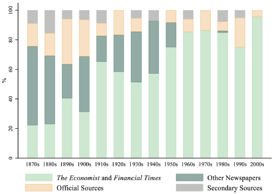
Figure 1 traces the historical share of each group of sources used in arriving at the final classifications. Prior to WWI, coverage in the Financial Times and The Economist was less extensive, and for this reason, we drew on a number of other newspapers from the British Newspaper Archive to form a more complete picture of the conditions that preceded each default. At the time, Britain was the world’s largest capital exporter, and its press frequently reported on international default events.

Figure 1 THE DISTRIBUTION OF SOURCES USED IN THE NARRATIVE IDENTIFICATION, 1870–2010

Notes: Other newspapers refer to other publications available in the British Newspaper Archive. Official reports include those from creditor organizations, government departments, and international institutions. Secondary sources include subsequent histories of state finances and academic studies of specific events.

Source: Online Appendix A.

For each default, we used a consistent narrative identification process. We began by exploring primary sources for the 12 months preceding the documented year of default. We do this for two reasons. The first is to enable us to classify the cause of each default, with the assistance of contemporary views from policymakers, the public, journalists, and stakeholders. In many cases, problems were apparent in the months leading up to the event. Where necessary, we also cross-checked our classification against the available secondary literature and investigated any discrepancies between contemporary opinion and its reconstruction by later authors. This step was mostly relevant for the earlier part of the sample. As many standard macroeconomic concepts and models were only introduced in the postwar period, we had to interpret the language of the sources in accordance with these models. Since these cases required more interpretation, we compared our classification to what specialists in the periods or countries involved have written about the crises in question.

The second reason for the pre-event window of 12 months was to uncover evidence of the anticipation of defaults by contemporaries. As we show later in the paper, deviations in the dating of debt crises can have a material impact on the estimates of aggregate default costs. In 31 percent of cases, we identify defaults that had either transpired or were known in the year prior to the date recorded in Reinhart and Rogoff (2011).

Even though we cannot exclude the possibility that contemporary reporting was clouded by stereotyping and creditor bias, the sources we consulted (both official reports and the press) were at pains to identify the underlying causes of defaults. Unbiased reporting was important for investors, who read the sources to ascertain how optimistic they should be about recovering any of their original funds. Indeed, sources such as The Economist and the Financial Times were independent (Butler and Freeman 1968) and trusted news outlets for financial market practitioners, who had an incentive to seek unbiased information (Hanna, Turner, and Walker 2020).

Before we describe our classification, it is important to acknowledge that other authors have addressed the endogeneity of output costs using different methods. Some papers have resorted to GMM (Furceri and Zdzienicka 2012; Esteves and Jalles 2016), while Kuvshinov and Zimmermann (2019) deal with the endogeneity of the default decision by conditioning on observables using an inverse propensity score weighted regression adjustment (IPSWRA). Finally, while the narrative approach has not been applied to sovereign debt crises before, other identification strategies used in the literature are nested within it, such as focusing on centrally orchestrated moratoria (Reinhart and Trebesch 2016) or on natural experiments, such as unexpected court rulings (Hébert and Schreger 2017).

Why Nations Default

Much has been written about the causes of defaults, with leading theoretical models emphasizing economic (Aguiar and Gopinath 2006; Arellano 2008) and non-economic (Cuadra and Sapriza 2008) factors. The literature also traditionally distinguishes between situations of inability and unwillingness to pay. The distinction is a relative one since the inability to pay is defined against the maximum social pain that can be imposed on citizens/taxpayers in order to honor the debt. This threshold can vary across nations and periods, such that two sovereigns can declare themselves unwilling or unable to repay similar debt flows. Nevertheless, creditors are more likely to protest or even retaliate against defaults perceived to be strategic or disconnected from the country’s economic fundamentals.⁴ Our own classification of defaults relates to these two categorizations. We recognize both economic and non-economic causes of defaults, and defaults driven by unwillingness to pay are a subset of those defaults we classify as exogenous to the business cycle.

From our reading of the narrative sources, we classified two types of endogenous debt crises and five types of exogenous crises. In the first group, we distinguish between crises driven by aggregate demand and aggregate supply shocks.⁵

Aggregate demand shocks (AD) reduce both output and prices, which can affect fiscal sustainability through growth, the real interest rate, and the primary balance. An example of this type of crisis is the Argentinean default of 1890, which contemporary opinion described as caused by a credit boom:

“Everyone can see that the growth has to a very large extent been a forced and unhealthy growth. Reckless borrowing and reckless expenditure have been the order of the day both with the Government and with the people, and the readiness with which European investors have responded to the never-ending appeals for new loans has done little credit to their intelligence. But the speculative bubble has now been pricked” (The Economist, 8 August 1890, p. 984).

Aggregate supply shocks (AS) reduce output and raise prices. For example, Chile defaulted in 1961 as natural disasters inflicted “severe but not total damage […] upon the region’s basic industry – agriculture” (Financial Times, 31 May 1960, p. 2), combined with labor unrest in the copper sector as “the companies are being pressed by workers who demand higher wages and a government which relies on copper for part of its revenue and demands a high rate of expansion in output” (The Economist, 19 August 1961, p. 742).

The five classes of plausibly exogenous debt crises/restructurings are: centrally orchestrated moratoria (CM), contagion (C), legal (L), political (P), and terms of trade shocks (T).

Centrally orchestrated moratoria (CM) include programs for debt relief for groups of indebted countries.⁶ There have been a number of debt relief initiatives in modern history, starting with the 1931 Hoover Moratorium, followed by the Baker and Brady plans of 1985 and 1989, as well as the more recent HIPC and MDRI initiatives. To the extent that the relief is independent of country-specific economic conditions, these moratoria are exogenous.

Contagion (C) occurs when a financial shock in one economy spills over into others, making debt more expensive or harder to roll over. While it is difficult to identify pure cases of contagion (Forbes and Rigobon 2002), the financial press was unanimous, for example, in attributing the Paraguayan and Uruguayan defaults of 2003 to the fallout from the 2001 Argentinian debt crises.

Legal (L) disputes over sovereign defaults have been on the rise in recent decades (Schumacher, Trebesch, and Enderlein 2021), and some authors have used their outcomes as external sources of variation for debt crises. For example, after Argentina defaulted in 2001 on debt issued under New York law, holdout creditors took the case to US courts, which ruled against Argentina, precipitating a technical default in 2014 (Hébert and Schreger 2017).⁷

Political (P) crises have been widely cited as causes of debt crises (Citron and Nickelsburg 1987; Brewer and Rivoli 1990; Balkan 1992; Kohlscheen 2007; Van Rijckeghem and Weder 2009; Oosterlinck 2016). Defaults can be associated with political events for a number of reasons. For our purposes, we are interested in cases where governments refuse to honor debt commitments for reasons unrelated to the burden of debt itself, such as ideology. From the perspective of creditors, these cases may be interpreted as a political “crisis,” even if a political movement has a democratic mandate to default. A recent example of this type of default is provided by the Ecuadorian default of 2008. Soon after being elected, the left-wing president, Rafael Correa, indicated his unwillingness to abide by some of the debt incurred by the previous right-wing government, even though the country was benefiting from a commodity boom and its foreign exchange reserves were higher than the principal of the affected debt at the time (Porzecanski 2010). In other instances, external intervention, such as occupation by foreign powers, forces countries into default. As reported by The Economist (21 January 1939, p. 134), following the Japanese occupation of China, “China wishes to pay all her obligations secured on the customs (derived from Japanese occupied areas) … but the Japanese authorities, in turn, have refused to make such payments.” Using changes in ideology and military events as exogenous shocks follows a long tradition in the fiscal policy literature (Ramey and Shapiro 1998; Romer and Romer 2010; Ramey 2011; Cloyne 2013; Crafts and Mills 2013, 2015; Ramey and Zubairy 2018).

Terms of trade (T) shocks may be another cause of sovereign debt crises, resulting from a general fall in the price of exports relative to imports or from the collapse (spike) in the price of one of the main commodities exported (imported). If these commodities are fiscally or economically important, then terms of trade shocks can undermine fiscal sustainability. For example, in 1932, Uruguay was “very largely dependent upon the meat industry; the extremely low prices of cattle have therefore been an adverse factor,” and a “diminution of revenues” accompanied the depression in trade (The Economist, 18 February 1933, p. 33). Similarly, a slump in the price of coffee pushed Venezuela into default in 1898 (Financial Times, 14 September 1897, p. 2). The assumption that terms of trade are exogenous to small open economies is “universally embraced by the related literature whether empirical or theoretical” (Schmitt-Grohé and Uribe 2018, p. 85).⁸

A final word about how we deal with cases with less-than-clear classification. Whenever there was joint evidence pointing to endogenous and exogenous causes, we conservatively classified the crises as endogenous. We show later in the paper that this classification is likely to bias our estimates downward.⁹ In four cases, there was not sufficient evidence to classify them either way, and we grouped them into a category of unclassified (U).

In Online Appendix A, we detail the evidence for our classifications of 174 sovereign debt crises between 1870 and 2010.

As a check of our ability to identify exogenous debt crises, we run two logit models of the form:

(4)

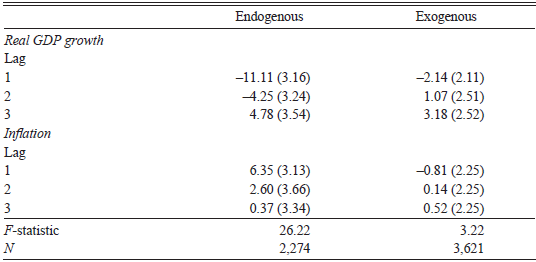
where is either the probability of an endogenous or exogenous crisis in country i at time t, α_i and γ_t are country and time fixed effects, Δy_i,t–k is lagged real GDP growth, and π_i,t–k is lagged inflation.¹⁰ The results are shown in Table 1. The endogenous series is highly predictable from lags of economic growth and inflation. The exogenous series, however, is not predictable.¹¹

Table 1 PREDICTING ENDOGENOUS AND EXOGENOUS CRISES

Notes: This table shows the results of a logit model of endogenous or exogenous defaults for 50 defaulting countries between 1870 and 2010 based on estimation of Equation (4). Standard errors are in parentheses.

Source: Authors’ calculations based on data described in the text.

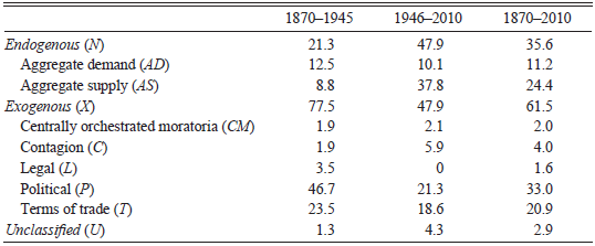
Table 2 shows the distribution of defaults by cause, according to our classification, for the whole period and for two sub-periods: before World War II (1870–1945) and since the war (1946–2010). Political events are the leading cause of default in our sample period, accounting for 1 in 3 episodes. Next in line are shocks to aggregate demand and supply, which together contributed a further third of defaults. Exogenous terms of trade shocks were present in 1 in 5 defaults. Centrally orchestrated moratoria, contagion, and legal crises have been less frequent.

Table 2 THE CAUSES OF SOVEREIGN DEBT CRISES, 1870–2010

Notes: This table summarizes the causes of sovereign debt crises in a sample of 50 defaulting countries between 1870 and 2010. Values in percent.

Sources: Online Appendix A and Reinhart and Rogoff (2011).

Table 2 also reveals two significant changes in the relative importance of certain categories of default. From the first to the second period, the share of political defaults falls by 25 percentage points, a drop that is matched by a rise in the share of defaults caused by AS shocks. The decline in the share of political defaults is not surprising, given the two world wars in the first half of the twentieth century and the subsequent absence of global conflicts in the postwar period. The increased share of AS shocks is partly due to the increase in the number of sovereigns. In the postwar era, a number of newly independent countries in Africa and Asia gained access to international debt markets. Many of these economies were producers of primary goods and commodities and exposed to natural shocks (Reinhart, Reinhart, and Trebesch 2016).

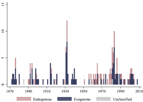
Overall, we classify 35.6 percent of defaults as endogenous and 61.5 percent as exogenous (2.9 percent remain unclassified). The significant share of endogenous crises suggests that simple OLS estimates of default costs may be materially biased. The evolution of endogenous, exogenous, and unclassified defaults is plotted in Figure 2. One particularly clear pattern is the clustering of exogenous defaults around major international financial crises, such as 1873, 1890, 1929–33, 1982–83, and 1997, as well as the two world wars. This clustering indirectly validates our narrative approach. Given the widespread nature of these crises, it is natural to expect to find more debt episodes around them that are exogenous to each country’s phase of the cycle.

Figure 2 DECOMPOSITION OF SOVEREIGN DEBT CRISES, 1870–2010

Notes: This figure shows a decomposition of sovereign debt crises into endogenous, exogenous, and unclassified categories for 50 defaulting countries between 1870 and 2010.

Sources: Online Appendix A and Reinhart and Rogoff (2011).

THE MACROECONOMIC EFFECTS OF SOVEREIGN DEBT CRISES

Model

In order to estimate the macroeconomic effects of sovereign debt crises, we run a lag-augmented local projections model (Jordà 2005; Montiel Olea and Plagborg-Møller 2021):

(5)

The subscripts i, t, and h index countries, time and horizon, respectively; y_i,t+h is the log of an economic outcome of interest; α_i,h and γ_t,h are country and time fixed effects; and X_i,t is a series of plausibly exogenous sovereign debt crises that equals 1 in the first year and 0 otherwise. We define sovereign crises by their initial year because the duration of defaults itself can be endogenous (Benjamin and Wright 2009). β_h is the treatment effect at each horizon. W_i,t is a vector of controls. The baseline model includes lags of the dependent and treatment variables and current and lagged measures of debt-GDP, the log change in the terms of trade, Polity scores, wars, and contagion.

We include controls for three reasons. First, to increase efficiency (Stock and Watson 2018). Second, in a long macro panel, there is a potential issue of non-stationarity that is obviated by including lags of the dependent variable as controls (Montiel Olea and Plagborg-Møller 2021).¹² Third, we suspect that a number of exogenous default categories may only be exogenous conditionally on controls, such as contagion (C), politics (P), and the terms of trade (T). While caused by plausibly random events, defaults of this kind may affect economic outcomes through channels other than default. Another way of saying this is to remember that some variables are potential confounders that might affect both the onset of a debt crisis and its outcomes. Failing to control for them would lead to omitted variable bias (Pearl 2009).

Data

To investigate the economic impact of sovereign debt crises, we assembled a dataset of outcome, treatment, and control variables for 50 defaulting economies from 1870. The variables, sources, description, and coverage are detailed in Online Appendix B.

The main outcome variable is real GDP. A valid concern is the reliability of historical national accounts. Even though we used the best available data, there are thought to be large margins of error prior to the Second World War, even for advanced economies (Solomou and Weale 1991). Nevertheless, as these data are used as outcomes, measurement error will most likely increase the standard errors but should not affect the consistency of the estimator.¹³ A related issue is whether historical GDP series are more appropriate for estimating growth trends than for identifying the timing and amplitude of business cycles. The latest vintage of historical GDP statistics used in this paper is based on detailed reconstructions of individual countries’ real GDP and has been used in a number of other papers on economic fluctuations.¹⁴ Moreover, we argue in Online Appendix D that it is unlikely the series are excessively smoothed.

The treatment variable is based on the chronology of sovereign debt crises compiled by Reinhart and Rogoff (2011). As controls, we include lags of the dependent and treatment variables, as well as current and lagged measures of debt-to-GDP, the log change in the terms of trade, Polity scores, wars, and contagion. We control for the pre-crisis debt burden because it is reasonable to expect that debt restructurings starting from very different debt-to-GDP ratios will differ in their consequences. The remaining controls are included to satisfy conditional exogeneity (Stock and Watson 2018).

As our measure of contagion is a proxy, it deserves some discussion. This variable is included to control for the possible impact of spillovers in one country from defaults in other countries (including instances when those spillovers do not lead to a local default). As two potential channels of contagion are capital and trade flows, which are known to be highly correlated with distance (Frankel and Rose 2002; Martin and Rey 2004; Portes and Rey 2005), we construct a measure based on distance from other defaults. Specifically,

(6)

where Default_j,t is a dummy variable indicating whether country j is in default, ω is a discount factor that is set to 0.999, and Distance_i,j is the great circle distance between the capital cities of countries i and j (Mayer and Zignago 2011). This measure has a number of useful properties: (i) if there are no crises, Contagion_i,t = 0; (ii) the more crises, the higher Contagion_i,t is; (iii) crises that are near are associated with higher Contagion_i,t than those that are far; (iv) Contagion_i,t is a concave up decreasing function of distance so that more local crises have a disproportionate impact compared to more distant crises.¹⁵

The geographic scope of our study includes countries that defaulted at least once between 1870 and 2010.¹⁶ The sample period begins in 1870, when macroeconomic data become increasingly available, and ends in 2010, when the series of sovereign debt crises stops (Reinhart and Rogoff 2011). Where possible, we collect data several years before and after each episode to allow us to include the leads and lags in Equation (5). For countries that gained independence after 1870, the sample begins in the year of independence. Overall, the sample consists of 5,476 country-years. Table 3 presents the summary statistics for the right- and left-hand side variables.

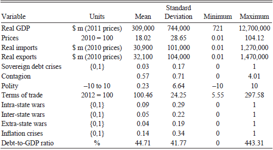
Table 3 SUMMARY STATISTICS

Notes: This table summarizes the data used in the main analysis.

Source: Authors’ calculations based on data described in the text.

Results

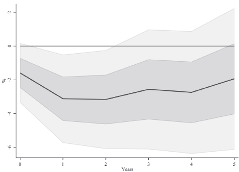
We estimate Equation (5) using least squares and one lag of the control variables.¹⁷ The solid line of Figure 3 plots the impulse response function of real GDP, together with one and two standard error bands based on heteroskedasticity-robust standard errors.¹⁸ In the aftermath of sovereign default, there is a moderate but statistically significant contraction in economic activity.¹⁹ On impact, output falls by 1.6 percent (t = –1.8), declining to 3.1 percent in year 1 (t = –2.4) and to 3.2 percent in year 2 (t = –2.2). However, the effect is no longer statistically different from zero by year three.

Figure 3 THE EFFECT OF SOVEREIGN DEBT CRISES ON REAL GDP

Notes: This figure shows the response of real GDP to plausibly exogenous sovereign default based on estimation of Equation (5) and a sample of 50 defaulting countries between 1870 and 2010. The shaded areas are one and two standard error bands based on robust standard errors.

Source: Authors’ calculations based on data described in the text.

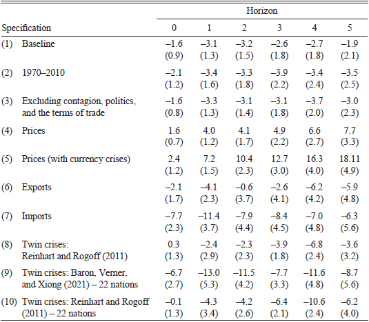
It is important to pause at this point and compare our estimates with those in the literature. It is fair to say that our results are on the lower end of those studies that find significantly negative and persistent effects of debt crises on GDP. Among the papers covering periods as long as ours, Reinhart and Rogoff (2009) estimate a larger loss than we do, starting at 3–4 percent on impact and rising to 5 percent over the medium run.²⁰ Our results are higher than the unconditional estimates of Tomz and Wright (2007), who calculated a GDP deviation of approximately 1.5 percent from trend in the wake of external debt crises. Two other papers concentrate on the post-1970 period. Furceri and Zdzienicka (2012) estimate costs of 6 percent of GDP on impact and 10 percent in the medium run, while Kuvshinov and Zimmermann (2019) found a loss of 3 percent on impact, peaking at 4.4 percent after 5 years and reverting to trend thereafter. To compare with the last two papers more easily, we re-estimate the model for the period from 1970 to 2010. The estimates reported in Table 4 are closer to Kuvshinov and Zimmermann’s (2019) as output falls by 2.1 percent on impact and bottoms at –3.9 percent after 3 years.

Table 4 THE EFFECT OF SOVEREIGN DEBT CRISES ON ECONOMIC OUTCOMES

Notes: This table shows the response (in percentage) of real GDP (rows 1, 2, 3, 8, 9, and 10), prices (4 and 5), or real trade flows (6 and 7) to plausibly exogenous sovereign default based on estimation of Equation (5). Robust standard errors are in parentheses.

Source: Authors’ calculations based on data described in the text.

However, it is not clear whether more recent defaults are more costly than historical ones. First, because the confidence intervals of the two IRFs overlap, it is unclear whether the two sets of estimates are significantly different or not. Second, as already noted, historical national accounts are more likely to be measured with error than modern estimates. Third, the presence of multilateral organizations that lend to countries in distress and in arrears is likely to affect the frequency and consequences of debt crises (Wells 1993). However, how these interventions affect our estimates is unclear. On the one hand, IMF lending can preempt debt crises. If the crises avoided tend to be the least serious, this would increase the estimated losses relative to a world without interventions. On the other hand, IMF lending after defaults could help mitigate the economic costs, which would bring down the size of the post-1970 estimates. The literature evaluating the outcomes of IMF programs is not conclusive, with some studies reporting a positive effect of IMF intervention on post-crisis macro outcomes and others finding a negative impact.²¹ Pre-1945, sovereigns rarely received official support from other nations to preempt debt crises.²² Finally, it is possible that the prevalence of debt crises short of formal defaults has grown over time. If crises associated with large hikes in spreads are less serious than those ending in defaults, we may be undercounting crises in the recent period and overstating their costs (Pescatori and Sy 2007; Krishnamurthy and Muir 2017).

As mentioned previously, defaults associated with contagion, politics, and the terms of trade may only be exogenous if we control for the direct effect of these factors on economic outcomes. For example, a change of political regime from democratic to autocratic may reduce growth by itself, irrespective of being associated with a default (Acemoglu, Naidu, Restrepo, and Robinson 2019). The importance of these controls is clear when they are dropped from the regression. The estimates of β _h in this short regression are similar to the baseline specification up to year 2 but are about 1 percentage point larger in absolute terms by year 5 (third row of Table 4).

Another interesting outcome is prices. Row 4 of Table 4 shows that price levels increase significantly and persistently after sovereign defaults: by 1.6 percent on impact (t = 2.4) and rising to 7.7 percent in year 5 (t = 2.4).²³ One possibility is that sovereigns, shut out from borrowing abroad and facing decreased revenues after a default, resort to inflationary funding (Reinhart and Rogoff 2009). An alternative explanation could be imported inflation. As defaults sometimes occurred in association with currency crises, large devaluations might translate into imported inflation. When we restrict the sample to defaults associated with currency crises, the effects on prices are twice as large as the baseline (row 5 of Table 4).

Mechanisms

Apart from comparing our results to the existing literature, we are also interested in investigating potential mechanisms for the aggregate economic loss following defaults. The literature on sovereign debt considers several mechanisms connecting crises in the sovereign sector to disruptions in the whole economy. An often-cited consequence of default is a contraction in international trade, either because trade credit tightens or because creditors punish defaulters with worse trade conditions (Rose 2005; Antràs and Foley 2015). A second mechanism operates through the sovereign risk channel (as measured by spreads) on the access to outside finance by the corporate sector, either through price rationing (Kaminsky and Schmukler 2002; Reinhart and Rogoff 2004; Das, Papaioannou, and Trebesch 2010) or credit rationing (Arteta and Hale 2008; Esteves and Jalles 2016). Theory provides several arguments for this mechanism. Bulow and Rogoff’s (1989) model justifies this with the overall penalty imposed on the sovereign. Other authors do not assume a reputational penalty from default but instead emphasize balance sheet effects (Guembel and Sussman 2009; Broner and Ventura 2010) or a negative revision of expectations about the growth potential of the economy in the context of a model with incomplete information (Cole and Kehoe 1998; Andrade 2009; Sandleris 2014).

Although it is challenging to test these many mechanisms with historical data, we investigate two of them here. First, we check directly for trade retrenchment by re-estimating Equation (5), substituting GDP with trade flows as the dependent variable. The results are reported in Table 4. We find a strong reaction of imports, which contract by 7.7 percent on impact, peaking at –11.4 percent after one year. The decline in exports is weaker: –2.1 percent on impact, peaking at –6.2 percent after 4 years. This implies that default brings about a current account reversal required to balance the external account, which is consistent with a number of other studies (Asonuma, Chamon, and Sasahara 2016; Kuvshinov and Zimmermann 2019).²⁴ In line with these papers, the brunt of the adjustment is taken by imports. This squeeze could reflect either a fall in the volume of final goods or intermediate inputs imported by firms. Even if export levels are less affected by a debt crisis, there is abundant evidence that defaults harm the export sector (Rose 2005; Borensztein and Panizza 2010). If a default is followed by tighter credit constraints on firms (Arteta and Hale 2008; Sandleris 2014; Esteves and Jalles 2016), they will have trouble acquiring imported inputs, reducing their efficiency and production (Mendonza and Yue 2012).

We then test for a second mechanism, domestic credit crunches, this time indirectly. We investigate the relationship between systemic banking crises and defaults. Kuvshinov and Zimmermann (2019) found that systemic banking crises that are triggered by defaults amplify the macroeconomic costs of debt crises.²⁵ We concentrate on banking crises that coincide with or start after plausibly exogenous defaults. This is to avoid situations where defaults are triggered by fiscal interventions to address issues in the banking sector. In other words, these estimates are not plagued by the endogeneity from the “diabolic loop” that often ties sovereigns and domestic banking sectors (Brunnermeier et al. 2016). This is only an indirect test of the mechanism as we restrict ourselves to extreme cases of disruption resulting in systematic banking crises. Since chronologies of banking crises have been criticized for “classification uncertainty” (Bordo and Meissner 2016), we use two datasets of systemic banking crises. The first, compiled by Reinhart and Rogoff (2011), covers all 50 nations in our sample. The second, by Baron, Verner, and Xiong (2021), is only available for a smaller subset of 22 economies between 1870 and 2010.

The impact of banking crises on the estimates is large and significant (see Table 4). Using Reinhart and Rogoff’s (2011) data leads to some attenuation of the short-run costs of defaults associated with systemic banking crises. However, the impulses are larger from year three, underscoring the concern that sovereign crises may destabilize the domestic financial sector. Including Baron, Verner, and Xiong’s (2021) chronology leads to much larger losses, but a significant share of this difference is due to the change in the sample composition, as can be seen by comparing rows 9 and 10 of Table 4.

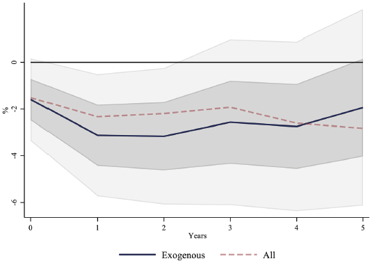
A major motivation for our narrative analysis is that the true cost of default is uncertain because of endogeneity. Therefore, a natural exercise is to compare the results of estimating Equation (5) for the restricted series of exogenous defaults and for the whole set of historical defaults. Figure 4 suggests that the qualitative result is the same, regardless of the sample: sovereign defaults lead to moderate and time-limited economic costs. However, the baseline estimates are more negative at short horizons but less so by year 5. The average difference between the two sets of estimates is 0.3 percent of GDP, with a maximum falling in year two when the baseline loss is larger by 1 percentage point. Why are the costs for the whole sample smaller? One possible explanation is that not all defaults are alike. It is to this question of heterogeneity that we now turn.

Figure 4 THE EFFECT OF SOVEREIGN DEBT CRISES ON REAL GDP: EXOGENOUS DEFAULTS VERSUS ALL DEFAULTS

Notes: This figure shows the response of real GDP to sovereign default based on estimation of Equation (5) and a sample of 50 defaulting countries between 1870 and 2010. The solid line is the baseline estimate. The dashed line is an alternative estimate based on all defaults. The shaded areas are one and two standard error bands based on robust standard errors.

Source: Authors’ calculations based on data described in the text.

Heterogeneity

Sovereign debt episodes are costly but are these costs contingent on the underlying driver of default? For example, centrally orchestrated moratoria are not designed to inflict economic damage but to lighten the burden of debt. To explore this possibility, we start by estimating a variant of Equation (5) that disaggregates the various sub-categories of default on the right-hand side:

(7)

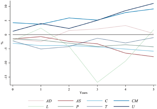
We plot the estimates of the coefficients associated with these sub-categories in Figure 5. Starting with endogenous crises, crises initiated after AD or AS shocks have the same immediate impact on GDP but differ markedly from year two. Whereas the path of GDP after AD-related crises recovers the initial losses, the aftermath of AS crises is consistently negative. As these shocks are endogenous, however, the results should be interpreted with caution.

Figure 5 THE EFFECT OF SOVEREIGN DEBT CRISES ON REAL GDP: HETEROGENEITY

Notes: This figure shows the response of real GDP to sovereign default by cause—aggregate demand shocks (AD), aggregate supply shocks (AS), contagion (C), centrally orchestrated moratoria (CM), legal (L), political (P), terms of trade (T), and unclassified (U)—based on estimation of Equation (7) and a sample of 50 defaulting countries between 1870 and 2010.

Source: Authors’ calculations based on data described in the text.

In terms of the exogenous crises, the most salient division is between debt restructurings initiated in the context of general moratoria and all other types of exogenous crises. As expected, moratoria have a consistently positive effect on economic activity, with output rising by 4.2 percent on impact and 9.1 percent after 5 years.²⁶ Debt crises after legal events have a wide amplitude of effects at different horizons; however, the estimates are based on a very limited number of cases. All other types of exogenous crises show a characteristic pattern of immediate and persistent negative impact, although the time pattern varies. Crises after terms of trade shocks, for instance, front-load economic costs relative to political crises, where output losses build up over time. Unclassified (U) defaults are typically associated with rising output.

Online Appendix C shows that the OLS estimate of the impact of sovereign default from all causes (the dashed line in Figure 4) can be expressed as a weighted average of the cause-specific effects in Equation (7):

(8)

where the weights are the cause-specific contribution to the frequency of defaults, and ϑ_h is a residual that captures the effects of covariates in the model.

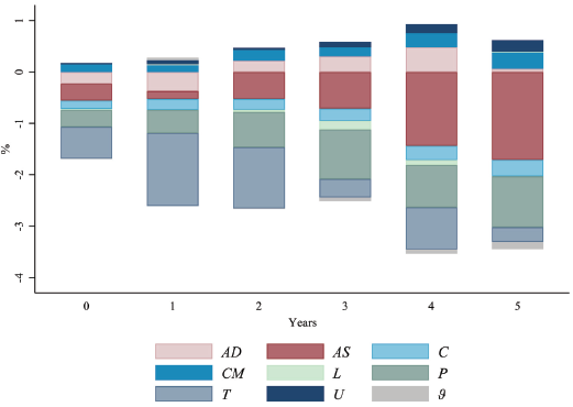
In Figure 6, we show the contribution of each type of episode to the OLS coefficient at different horizons. At short horizons, including all crises reallocates weight from contractionary exogenous causes such as politics and the terms of trade to less depressive endogenous types. At longer horizons, however, aggregate supply shocks dominate, which helps to explain why the OLS results become more negative than the narrative estimates.

Figure 6 ACCOUNTING FOR THE OLS ESTIMATE OF β_h

Notes: This figure shows a breakdown of the OLS estimate of β_h by cause—aggregate demand shocks (AD), aggregate supply shocks (AS), contagion (C), centrally orchestrated moratoria (CM), legal (L), political (P), terms of trade (T), and unclassified (U)—based on Equations (5), (7), and (8), and a sample of 50 defaulting countries between 1870 and 2010.

Source: Authors’ calculations based on data described in the text.

In general, this exercise underlines the heterogeneity of debt crises by their causes. Apart from moratoria, which have an expected positive impact, we find that crises initiated by pure demand shocks lead to relatively mild contractions that are quickly reversed. Shocks that affect domestic productivity or that impair the competitiveness of the traded sector have more negative and persistent effects.

ROBUSTNESS

In this section, we investigate whether our results are sensitive to sample composition, crisis classifications, default chronologies, and control variables.

Alternative Samples

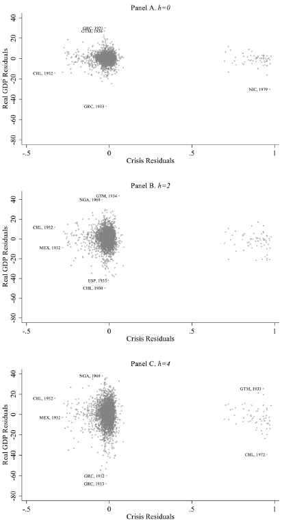
To control for the influence of outliers, we start by plotting the partial association between real GDP and plausibly exogenous crises.²⁷ Figure 7 shows the results for horizons of 0, 2, and 4 years. The real GDP residuals are scattered on the y-axis along with the crisis residuals on the x-axis. As our variable of interest is a dummy variable, the points are scattered around 0 and 1 along the x-axis. The largest outliers are labeled to help identify the most extreme times and places.

Figure 7 PARTIAL ASSOCIATION OF REAL GDP AND SOVEREIGN DEBT CRISES

Notes: This figure shows the partial association between real GDP at horizons t + h and plausibly exogenous debt crises at time t based on variants of Equation (5) and a sample of 50 defaulting countries between 1870 and 2010.

Source: Authors’ calculations based on data described in the text.

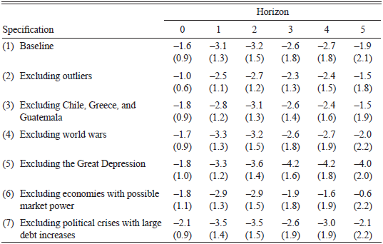
To explore how the identified outliers might influence our results, we estimate a number of additional specifications reported in Table 5. The first drops the outlier cases labeled in Figure 7. The second removes the common outlying countries: Chile, Greece, and Guatemala. The third and fourth omit potential outlying periods: the world wars (1914–8 and 1939–45) and the Great Depression (1931–3). Excluding extreme observations slightly reduces the estimated maximum effects. Excluding outlying countries and the world wars hardly affects the peak losses. Interestingly, excluding the Great Depression increases the estimated peak impact. This may confirm Lindert and Morton’s (1989) conclusion that the costs of defaults are lower when countries default together rather than in isolation. The 1930s had the largest concentration of defaults in the sample period.²⁸ Despite these variations, the impulse responses are statistically significant at most horizons in all cases.

Table 5 THE EFFECT OF SOVEREIGN DEBT CRISES ON REAL GDP: ALTERNATIVE SAMPLES

Notes: This table shows the response (in percentage) of real GDP to plausibly exogenous sovereign default based on estimation of Equation (5) and alternative samples. Robust standard errors are in parentheses.

Source: Authors’ calculations based on data described in the text.

The last two rows of Table 5 test the robustness of the results to two classification questions. First, the terms of trade might not be exogenous for economies that are large in global markets. In these cases, domestic supply shocks could affect export prices, which would undermine the exogeneity of any subsequent debt crisis. In our narrative classification, we only defined a default as caused by a terms of trade shock if the sources described it as unrelated to domestic shocks. Nevertheless, we experimented with excluding the countries for which Blattman, Hwang, and Williamson (2007) question the exogeneity of the terms of trade. This includes the core economies of Austria, Germany, Italy, and the United Kingdom due to a high degree of market power, and the periphery of Brazil, Chile, China, India, the Philippines, and Russia, as they produced more than one-third of the global share of exports in a commodity and/or more than 5 percent of global exports. The losses reported in row 6 of Table 5 are slightly larger upon impact but marginally smaller thereafter. A second concern involves the classification of political defaults. We identified these cases when the sources did not associate political strife with the business cycle or significant debt accumulation. To confirm that our interpretation of the sources does not bias the results, we computed the change in debt-to-GDP in the five years before defaults. We then identified eight politically-driven defaults that were in the top quartile for debt accumulation. The last row in Table 5 shows that the results are robust to the removal of these episodes.

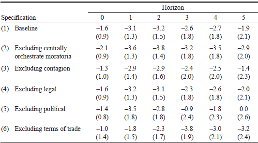
Moratoria are, by their very nature, different from other debt crises. Indeed, moratoria can avert debt crises and decrease the aggregate costs of debt restructuring. Despite the fact that debt crises associated with moratoria are included in all the standard default chronologies, we attempt here to separate the two. If we exclude defaults associated with centrally orchestrated moratoria from the sample, we obtain costs that are larger than the baseline results by 0.5 to 1 percentage points (second row of Table 6), consistent with the positive impact of moratoria on GDP that we identified in Figure 5. As a further exercise, we re-run Equation (5), leaving one exogenous sub-category out at a time from the sample. Table 6 shows that the baseline results are robust to all of these exclusions.

Table 6 THE EFFECT OF SOVEREIGN DEBT CRISES ON REAL GDP: EXCLUDING CATEGORIES OF DEFAULTS

Notes: This table shows the response (in percentage) of real GDP to plausibly exogenous sovereign default based on estimation of Equation (5), alternative classifications, and a sample of 50 defaulting countries between 1870 and 2010. Robust standard errors are in parentheses.

Source: Authors’ calculations based on data described in the text.

Alternative Classifications

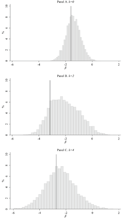
An important question is how accurate our classification is. In order to benchmark the potential bias from misclassification, we reclassify a random fraction of crises as exogenous or endogenous.²⁹ Figure 8 shows the distribution of estimated impulse responses for horizons 0, 2, and 4. At years 0 and 4, the distribution is centered around the baseline estimates. At horizon 2, the distribution is centered at a lower estimate than the baseline, but even there, the mass is clearly negative. This is remarkable since some of the simulated estimates result from assuming improbably large rates of misclassification.

Figure 8 THE DISTRIBUTION OF β_h: TWO-WAY RECLASSIFICATION

Notes: This figure shows the distribution of β_h from 10,000 runs, where crises are randomly reclassified from endogenous to exogenous or from exogenous to endogenous, based on estimation of Equation (5) and a sample of 50 defaulting countries between 1870 and 2010. The black line is the baseline estimate. Outliers have been dropped for clarity.

Source: Authors’ calculations based on data described in the text.

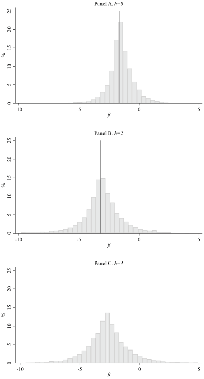
Another possibility is that the errors in our classification are not random but systematic. It could be argued that by focusing on American and British sources, the reporting may be biased in favor of the creditors. This may translate into an endogenous crisis being misreported as exogenous. For example, if a drought caused a severe recession and, with it, the inability of the government to honor its debt commitments, the foreign press, pandering to Western creditors, could interpret default as a political choice. This is an unlikely possibility for several reasons. First, investors would have little to gain from being misled about the underlying fiscal capacity of the defaulter and would favor trusted sources. Second, we have cross-referenced the accounts from primary sources with those from secondary sources. Third, Table 1 suggests that exogenous crises are unpredictable, while endogenous crises are highly predictable, which implies that crises are not systematically misclassified. In any case, it is possible to bring further evidence to bear on the matter by randomly reclassifying a fraction of exogenous crises as endogenous. Figure 9 shows that the distribution of impulse responses is also centered on the baseline estimates.³⁰

Figure 9 THE DISTRIBUTION OF β_h: ONE-WAY RECLASSIFICATION

Notes: This figure shows the distribution of β_h from 10,000 runs, where crises are randomly reclassified from exogenous to endogenous, based on estimation of Equation (5) and a sample of 50 defaulting countries between 1870 and 2010. The black line is the baseline estimate. Outliers have been dropped for clarity.

Source: Authors’ calculations based on data described in the text.

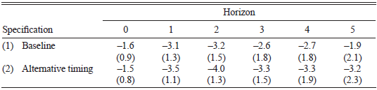
A reliable record of crises is vital to estimate the macroeconomic effects of defaults. In the baseline model, we have used Reinhart and Rogoff’s (2011) latest chronology. In the process of our narrative analysis, however, we noticed a number of instances where the news of a default was reported prior to the date recorded by Reinhart and Rogoff (2011). A potential concern is that if a default was anticipated, the economic effects may start before the recorded onset, potentially biasing the impulse response functions. To address this issue, we adjust the timing of X_i,t to match the narrative record. As shown in the second row of Table 7, the estimate of the crisis effect is slightly lessened on impact but increases over the other horizons, which suggests that the low frequency of standard default chronologies (annual) may lead to an underestimation of the aggregate default costs.

Table 7 THE EFFECT OF SOVEREIGN DEBT CRISES ON REAL GDP: ALTERNATIVE CLASSIFICATION

Notes: This table shows the response (in percentage) of real GDP to plausibly exogenous sovereign default based on estimation of Equation (5) and an alternative classification. Robust standard errors are in parentheses.

Source: Authors’ calculations based on data described in the text.

Alternative Control Variables

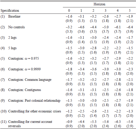
An econometric model must strike a balance between possible omitted variable bias and the lost degrees of freedom arising from saturation. In this section, we investigate how variations in the control vector, W_i,t, influence our results. Specifically, we experiment with three changes to the vector of controls: removing controls, adding controls, and changing the definition of the only constructed control (contagion). In the last case, we tried varying the weight on distance (to ω = 0.975 and ω = 0.9999) and substituting geographical distance with alternative proxies for distance, such as sharing a common official or primary language, a border, or a past colonial relationship.³¹ In the models with extended controls, we experimented with increasing the lag length to 2 years and 5 years (based on the minimization of the Akaike and Bayesian information criteria) and with controlling for other crises (banking, currency, domestic debt, and inflation), which could be twinned with sovereign debt crises and associated with economic fluctuations.³² We also control for current account reversals, which we use to test for the influence of global capital cycles. In the absence of good data on the financial accounts for all nations over the long period we study, we resort to the database of current account reversals constructed by Adalet and Eichengreen (2007) as mirror measures of sudden capital stops.³³

The results are presented in Table 8. In most variants, the estimated peak losses are largely unaffected. The only exceptions are when we omit all controls and include current account reversals, when the peak costs rise, and when we control for other crises, when the costs fall. In all cases, the responses are economically and statistically significant in the aftermath of sovereign debt crises.

Table 8 THE EFFECT OF SOVEREIGN DEBT CRISES ON REAL GDP: ALTERNATIVE CONTROL VARIABLES

Notes: This table shows the response (in percentage) of real GDP to plausibly exogenous sovereign default based on estimation of Equation (5) and a sample of 50 defaulting countries between 1870 and 2010. Robust standard errors are in parentheses.

Source: Authors’ calculations based on data described in the text.

However, this reasoning only applies to observable controls. We cannot rule out that some unobservable variable is also relevant. Diegert, Masten, and Poirier (2023) derived a test to assess the sensitivity to omitted variable bias when the controls are potentially endogenous. A key test statistic is the breakdown point, defined as “the largest magnitude of selection on unobservables relative to observables needed to overturn a specific baseline finding.” In our case, the breakdown point varies between 38.7 percent (on impact) and 49.4 percent (2 years after) in the interval where the baseline results are statistically significant. This implies that the true impact of defaults is negative as long as selection on unobservables is at most 49.4 percent as large as selection on observables. Since this is only a relative quantity, we follow the suggestion of Diegert, Masten, and Poirier (2023) to compare the breakpoints with a measure of the importance of each included variable relative to all observed covariates. In all but one case, the breakpoints are larger than these individual measures, suggesting that our results are robust to omitted variables.³⁴

CONCLUSION

In this paper, we provide new evidence on the aggregate costs of sovereign debt episodes in modern history, covering 50 nations over 140 years. To our knowledge, we are the first to address the endogeneity of default using the narrative method. Our estimates are similar to, if a little lower than, other studies that find a significant and persistent impact of defaults on economic activity. Output losses start at 1.6 percent of GDP on impact, rise to 3.2 percent after two years, and return to zero after five years. One reason for our lower estimates is the extended sample we study. Consistent with some recent papers, we find larger losses for defaults occurring since 1970. The fact that our results are consistent with what other authors have found using different methods is indicative of the external validity of our approach over the longer time horizon.

An advantage of the narrative approach is that it has fewer data requirements than alternative methods used in the literature to control for the endogeneity of debt crises, such as GMM or propensity score matching. Consistent and reliable narrative sources are available from early on and allow us to extend the time coverage of our study as far back as the available series of real GDP for the 50 nations included in the sample.

A second advantage is that the narrative approach allows us to explore the heterogeneity of debt episodes. Our classification of defaults reveals a large heterogeneity of costs by the cause of default. Higher costs are associated with defaults initiated by shocks to the underlying productivity or competitiveness of an economy (domestic supply shocks, political crises, adverse terms of trade shocks). At the other extreme, countries that default as part of centrally orchestrated moratoria experience a significant boost to their output up to five years after, which is consistent with the debt relief aim of these programs. Between these extremes, we find that defaults associated with aggregate demand shocks, legal rulings, or contagion have moderately negative or no effect on the path of GDP post default.

Our results underscore that heterogeneity may be a greater obstacle to benchmarking the costs of defaults than endogeneity. This can be particularly relevant for theoretical research that calibrates the typical costs of default from particular debt episodes.

Exploring the heterogeneity of defaults also allows us to break down the sources of the potential endogeneity bias in the estimation of the aggregate costs of debt crises. Other methods correct the bias but do not allow for its decomposition. We found an endogeneity bias averaging 0.3 percent of GDP over the five years after a default (with a maximum of 1 percent after two years). Contrary to expectations, OLS underestimates the aggregate costs of a default up to four years after each episode. Whereas it is intuitive to expect that endogenous defaults would bias the estimated costs upward, the evidence is mixed. Our analysis shows that this is due to the backloading of the impact of endogenous shocks. Unlike other shocks, crises initiated on the domestic supply side have cumulative effects that dominate the impulse response from year four after a default.

In terms of mechanisms, we identify a distinct current account reversal lasting five years. Consistent with previous research, we also find that default episodes that trigger subsequent banking crises have larger aggregate costs, underscoring the concern that debt crises can destabilize domestic banks and lead to credit crunches.

Finally, our results survive a number of robustness checks: sample composition, outliers, choice of covariates, and classification of crises. Perhaps the most interesting result from these is the significant impact of the dating of defaults. In our work with narrative sources, we came across a number of instances where the news of default was reported prior to the date recorded in the standard chronologies. Correcting for this appears to increase the estimated costs. Further research on how to define and date sovereign debt episodes is clearly needed.