


1. Introduction
Stably stratified (vertical) shear flows, where both the background fluid buoyancy (i.e. the appropriately scaled negative density perturbation) and horizontal flow velocity vary with height, are ubiquitous in geophysical contexts. There has been a very large body of work considering the ways in which such flows behave (as evidenced by a sequence of reviews such as Fernando (Reference Fernando1991), Peltier & Caulfield (Reference Peltier and Caulfield2003), Ivey, Winters & Koseff (Reference Ivey, Winters and Koseff2008), Caulfield (Reference Caulfield2020) and Caulfield (Reference Caulfield2021)), with significant focus on the (possible) existence of turbulence extracting and converting the kinetic energy in the background shear and the associated enhanced (irreversible) turbulent mixing. Understanding (and parameterising) such turbulent mixing of stratified fluids is a key challenge in geophysical flows, as the transport of momentum, heat and other scalars (such as dissolved gases, pollution and microplastics for example) is both a crucial process and a phenomenon of great uncertainty for the description of the world’s climate and environment (see for example the reviews of Wunsch & Ferrari (Reference Wunsch and Ferrari2004), Ferrari & Wunsch (Reference Ferrari and Wunsch2009) and Gregg et al. (Reference Gregg, D’Asaro, Riley and Kunze2018)).
In essence, as shown schematically in figure 1, stably stratified shear flows are characterised by a competition between a stabilising buoyancy and a de-stabilising velocity (or shear) profile. However, gaining an understanding of fundamental aspects of this deceptively simple set-up continues to prove exceptionally complicated. Considering initial-value problems of (initially) laminar velocity and density profiles, it is well known that such flows can be prone to a range of primary flow instabilities (see the review of Caulfield Reference Caulfield2021) that effectively rearrange the strip of spanwise vorticity into trains of elliptical vortices (such as the classic Kelvin–Helmholtz ‘billows’, i.e. the saturated manifestation of the Kelvin–Helmholtz instability (KHI)). As these vortices themselves are prone (at least for sufficiently high Reynolds number) to a ‘zoo’ of secondary instabilities (a nomenclature proposed by Mashayek & Peltier Reference Mashayek and Peltier2012a , Reference Mashayek and Peltierb ), turbulence transition is triggered and mixing as well as dissipation are eventually significantly enhanced.
Such mixing events can extend for a significant length of time – particularly when the flow is prone primarily to the so-called ‘Holmboe wave instability’ (HWI) (Holmboe Reference Holmboe1962), as discussed in detail by Salehipour et al. (Reference Salehipour, Caulfield and Peltier2016, Reference Salehipour, Peltier and Caulfield2018) – and can also be accompanied by the formation of larger-scale emergent structures, especially in sufficiently spatially extended flow domains (Watanabe & Nagata Reference Watanabe and Nagata2021). The particular life cycle of such mixing events can be strongly sensitive to initial conditions, as demonstrated conclusively by Liu, Kaminski & Smyth (Reference Liu, Kaminski and Smyth2022), due to competition between different members of the secondary instability ‘zoo’, especially involving the subharmonic ‘pairing’ instability of neighbouring primary Kelvin–Helmholtz billows. As demonstrated by Mashayek & Peltier (Reference Mashayek and Peltier2013), sufficiently strong stratification can disrupt and hence suppress such pairing (or more precisely ‘merging’) events due to the energetic costs of the inherent vertical motions. Given only finite computational resources, such suppression is often cited as a reason to restrict (the inevitably finite) domains to one (or at most two) wavelengths of the primary instabilities, allowing for higher Reynolds numbers.
However, the horizontal extent of the (numerical or experimental) domain may clearly affect the flow dynamics. As shown by Scinocca & Ford (Reference Scinocca and Ford2000), a rich dynamics can occur in longer streamwise domains, where primary instabilities with close wavelengths (and hence close linear growth rates) can compete as they grow to finite amplitude if the (conventional) imposition of periodic streamwise boundary conditions does not quantise the accessible wavelengths of possible instabilities too severely. Analogous issues also arise in the spanwise direction. Many studies consider relatively narrow domains, in the sense that the spanwise extent is (often significantly) smaller than the characteristic (streamwise) wavelength of the primary instability. Such domains allow many of the (essentially local) secondary instabilities to develop and hence trigger turbulence transition. However, as can be straightforwardly observed in sufficiently wide tilting tank experiments (Thorpe Reference Thorpe1985, Reference Thorpe1987; Caulfield, Yoshida & Peltier Reference Caulfield, Yoshida and Peltier1996; Thorpe Reference Thorpe2002) and sufficiently wide computational domains, as clearly demonstrated by Fritts et al. (Reference Fritts, Lund and Thorpe2022a , Reference Fritts, Wang, Thorpe and Lundb ), inherently three-dimensional ‘knots’, ‘tubes’ and billow ‘defects’ can develop in the spanwise direction on scales of the order of (but typically larger than) the primary instability’s most unstable streamwise wavelength.

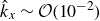
Figure 1. Configuration of the forced stratified shear flows considered here. While the initial buoyancy profile $b_{0}$
is statically stable, the imposed initial velocity profile
$b_{0}$
is statically stable, the imposed initial velocity profile $u_{x, 0}$
may induce flow instabilities that lead to a transition to turbulence. A continuous forcing
$u_{x, 0}$
may induce flow instabilities that lead to a transition to turbulence. A continuous forcing $f_{\varPhi }$
may inject the required energy to sustain this turbulence, ensuring statistically stationary dynamics.
$f_{\varPhi }$
may inject the required energy to sustain this turbulence, ensuring statistically stationary dynamics.
Moreover, there will always be an inevitable decay of these reported flow structures unless the underlying driving mechanism (i.e. the shear) is replenished. Although such initial-value-problem mixing events are undoubtedly of geophysical interest and indeed demonstrate the formation of a transient larger-scale dynamics exhibiting the so-called ‘life cycle’ of a shear-driven mixing event, it is important to remember that such initial-value-problem mixing events are really just one end-member class of the possible flows of geophysical interest.
The other obvious end-member class is the class of continuously forced flows, where the ‘background’ velocity and density (or equivalently buoyancy) profiles are driven by some external, quasi-steady forcing. Possible candidate mechanisms for such geophysically relevant forcings include wind, solar radiation and resulting evaporation at the surface of the ocean (Thorpe Reference Thorpe2005), tidal forcing (Laurent, Simmons & Jayne Reference Laurent, Simmons and Jayne2002), active matter living in water (Castro et al. Reference Castro, Pena, Nogueira, Gilcoto, Broullon, Comesana, Bouffard, Garabato and Mourino-Carballido2022) or continuous outflows from rivers (Uncles & Mitchell Reference Uncles and Mitchell2011). While this list is not meant to be complete in any sense, it illustrates that quasi-steady forcings do occur in geophysically relevant situations. An (artificial) volumetric forcing is a particularly convenient way to mimic these natural complex mechanisms in a simplified manner. As visualised on the right side of figure 1, such a forcing may be defined to relax the time-dependent local profiles.
Such a forcing was introduced by Smith, Caulfield & Taylor (Reference Smith, Caulfield and Taylor2021), who demonstrated that – after an initial transient where primary instabilities (either KHI or HWI) develop and (inevitably) break down – the ensuing turbulence could be sustained over arbitrarily long times, thus enabling statistically steady statistics of the flow to be calculated. There is a clear attraction to considering such forced flows due principally to the inherent removal of the confounding effects of the life cycle of the mixing event from the turbulence statistics. Therefore, such flows seem the natural test bed to study the emergent and sustained turbulent self-organisation of the flow on large scales. This endeavour, however, comes necessarily with the challenge of first diagnosing whether or not there is actually an inherent convergence of the resulting depth of the turbulent shear layer, and second, identifying its minimal required extent to enable such statistical convergence (that is unbiased by the extent of the domain).
Given that Smith et al. (Reference Smith, Caulfield and Taylor2021), similar to the initial-value-problem flows discussed above, also considered relatively small computational domains only, it is not at all clear whether or not their statistically stationary flow remained unaffected by the computational domain size. An equivalent question to ask is ‘what are the unconstrained emergent length scales of a forced stratified shear flow?’ Answering that (open) question is the central objective of this paper.
To address this objective, the rest of the paper is organised as follows. In § 2 we present our numerical approach before we list the range of considered control parameters and computational domains at the start of § 3. For simplicity, we focus on one set of parameters that enables a relatively weakly stratified flow which is prone to primary KHI. After briefly identifying some interesting early-time dynamics that may possibly be affected by molecular diffusion due to the choice of control parameters (but is not of principal interest here), we shift our focus to the statistically steady turbulent state that is sustained by the volumetric forcing. We identify emergent, strongly anisotropic length scales which are proven to converge in sufficiently extended domains. We demonstrate conclusively that key statistics of the flow, including in particular those related to irreversible mixing, are sensitive to the large-scale self-organisation of the flow or equivalently the extent of the computational domain. From a practical perspective, we remark that for convergent statistics, perhaps surprisingly, the flow domain may need to be extraordinarily extended (i.e. of order $100$
times larger) compared with the initial shear layer half-depth. Focusing on the flow physics, in § 4 we propose the dynamical origin of and discuss the implications of the discovered emergent large-scale dynamics. Finally, we draw our conclusions in § 5.
$100$
times larger) compared with the initial shear layer half-depth. Focusing on the flow physics, in § 4 we propose the dynamical origin of and discuss the implications of the discovered emergent large-scale dynamics. Finally, we draw our conclusions in § 5.
2. Numerical approach
2.1. Governing equations
We consider an incompressible flow based on the Oberbeck–Boussinesq approximation with a linear equation of state. The three-dimensional equations of motion are non-dimensionalised using the (dimensional) initial magnitudes of the streamwise velocity $U_{0}$
and buoyancy
$U_{0}$
and buoyancy $B_{0}$
, as well as the shear layer half-depth
$B_{0}$
, as well as the shear layer half-depth $d_{0}$
, as shown in figure 1. Using the advective time scale
$d_{0}$
, as shown in figure 1. Using the advective time scale $\tau _{\textit{ad}v} := d_{0} / U_{0}$
and the appropriate characteristic pressure scale
$\tau _{\textit{ad}v} := d_{0} / U_{0}$
and the appropriate characteristic pressure scale $p_{\textit{char}} := U_{0}^{2} \rho _{\textit{ref}}$
, where
$p_{\textit{char}} := U_{0}^{2} \rho _{\textit{ref}}$
, where $\rho_{ref}$
is a reference density, non-dimensional variables (marked here with a tilde) can be related to the dimensional variables as follows:
$\rho_{ref}$
is a reference density, non-dimensional variables (marked here with a tilde) can be related to the dimensional variables as follows:
 \begin{equation} \boldsymbol{x} = d_{0} \tilde {\boldsymbol{x}} , \qquad \boldsymbol{u} = U_{0} \tilde {\boldsymbol{u}} , \qquad b = {B_{0}} \tilde { b } , \qquad t = \tau _{\textit{ad}v} \tilde { t } , \qquad p = p_{\textit{char}} \tilde { p }. \end{equation}
Henceforth, we focus on non-dimensional variables, and so drop the tildes from all variables.
As a consequence, the non-dimensional governing equations are
 \begin{align} \boldsymbol{\nabla }\boldsymbol{\cdot }\boldsymbol{u} &= 0 , \end{align}
 \begin{align} \frac {\partial \boldsymbol{u}}{\partial t} + \left ( \boldsymbol{u} \boldsymbol{\cdot }\boldsymbol{\nabla }\right ) \boldsymbol{u} &= - \boldsymbol{\nabla }p + \frac {1}{\textit{Re}_{0}} {\nabla} ^{2} \boldsymbol{u} + \textit{Ri}_{0} b \boldsymbol{e}_{z} + f_{u} \boldsymbol{e}_{x} , \end{align}
 \begin{align} \frac {\partial b}{\partial t} + \left ( \boldsymbol{u} \boldsymbol{\cdot }\boldsymbol{\nabla }\right ) b &= \frac {1}{\textit{Re}_{0} {\textit{Pr}}} {\nabla} ^{2} b + f_{b} , \end{align}
where $\boldsymbol{u}$
,
$\boldsymbol{u}$
, $b$
and
$b$
and $p$
represent the velocity, buoyancy and modified pressure field, respectively. The precise form of the volumetric forcing terms
$p$
represent the velocity, buoyancy and modified pressure field, respectively. The precise form of the volumetric forcing terms $f_{u}$
and
$f_{u}$
and $f_{b}$
will be defined below. The buoyancy
$f_{b}$
will be defined below. The buoyancy $b := - \rho ^{\prime } g / \rho _{\textit{ref}}$
, where
$b := - \rho ^{\prime } g / \rho _{\textit{ref}}$
, where $g$
is the acceleration due to gravity, corresponds to the negative of the reduced gravity, so
$g$
is the acceleration due to gravity, corresponds to the negative of the reduced gravity, so $\rho '$
is the deviation from
$\rho '$
is the deviation from $\rho _{\textit{ref}}$
. Three non-dimensional parameters naturally emerge from this scaling: the Prandtl number, the initial bulk Reynolds number and the initial bulk Richardson number,
$\rho _{\textit{ref}}$
. Three non-dimensional parameters naturally emerge from this scaling: the Prandtl number, the initial bulk Reynolds number and the initial bulk Richardson number,
 \begin{equation} {\textit{Pr}} := \frac {\nu }{\kappa } , \qquad \textit{Re}_{0} := \frac {U_{0} d_{0}}{\nu } , \qquad \textit{Ri}_{0} := \frac {{B_{0}} d_{0}}{U_{0}^{2}} , \end{equation}
respectively, where $\nu$
is the kinematic viscosity and
$\nu$
is the kinematic viscosity and $\kappa$
is the buoyancy diffusivity. We restrict our attention to statically stable situations where
$\kappa$
is the buoyancy diffusivity. We restrict our attention to statically stable situations where $\textit{Ri}_{0} \gt 0$
.
$\textit{Ri}_{0} \gt 0$
.
The volumetric forcing terms $f_{u}$
and
$f_{u}$
and $f_{b}$
in (2.3) and (2.4) are a crucial aspect of our configuration. Following Smith et al. (Reference Smith, Caulfield and Taylor2021), we consider
$f_{b}$
in (2.3) and (2.4) are a crucial aspect of our configuration. Following Smith et al. (Reference Smith, Caulfield and Taylor2021), we consider
 \begin{align} f_{u} &:= - \frac {1}{{t_{{r}}}} [ u_{x} {-} u_{x, 0} ] \quad \mathrm{with} \quad u_{x, 0} (z) := \tanh (z) , \end{align}
 \begin{align} f_{b} & := - \frac {1}{{t_{{r}}}} [ b {-} b_{0} ] \qquad\, \mathrm{with} \quad b_{0} (z) := \tanh ( {R_{0}} z ), \end{align}
where $t_{{r}}$
is the response time while
$t_{{r}}$
is the response time while $u_{x, 0}$
and
$u_{x, 0}$
and $b_{0}$
represent the initial streamwise velocity and buoyancy base profiles to which the flow relaxes back under the effect of the forcing, at least in principle. In this context,
$b_{0}$
represent the initial streamwise velocity and buoyancy base profiles to which the flow relaxes back under the effect of the forcing, at least in principle. In this context, ${R_{0}} := d_{0} / \delta _{0}$
defines the ratio of initial interface half-depths (i.e.
${R_{0}} := d_{0} / \delta _{0}$
defines the ratio of initial interface half-depths (i.e. $\delta _{0}$
represents the dimensional initial buoyancy interface half-depth) with
$\delta _{0}$
represents the dimensional initial buoyancy interface half-depth) with ${R_{0}} = \sqrt {{\textit{Pr}}}$
following the diffusive arguments presented by Smyth, Klaassen & Peltier (Reference Smyth, Klaassen and Peltier1988). In essence, these forcing terms are idealised models of geophysically relevant processes (see again our introduction) that tend to restore the initial profiles
${R_{0}} = \sqrt {{\textit{Pr}}}$
following the diffusive arguments presented by Smyth, Klaassen & Peltier (Reference Smyth, Klaassen and Peltier1988). In essence, these forcing terms are idealised models of geophysically relevant processes (see again our introduction) that tend to restore the initial profiles $u_{x, 0}$
and
$u_{x, 0}$
and $b_{0}$
, and thus sustain turbulence over arbitrarily long times. In this context, we stress that the response time
$b_{0}$
, and thus sustain turbulence over arbitrarily long times. In this context, we stress that the response time $t_{{r}}$
quantifies the relative strength (or rather weakness) of these superposed processes. While
$t_{{r}}$
quantifies the relative strength (or rather weakness) of these superposed processes. While ${t_{{r}}} \rightarrow 0$
implies vigorously enforcing the sharp initial profiles,
${t_{{r}}} \rightarrow 0$
implies vigorously enforcing the sharp initial profiles, ${t_{{r}}} \rightarrow \infty$
corresponds to the disappearance of the forcing. As shown by Smith et al. (Reference Smith, Caulfield and Taylor2021), the broad sweetspot – to allow for sustained turbulence without prescribing a significant signal of the forcing – lies in between and tends to preserve the primary instability associated with the underlying base profiles. Finally, we remark that, although the included base profiles are time-independent, the resulting rate of momentum or buoyancy injection is typically not constant in space or time.
${t_{{r}}} \rightarrow \infty$
corresponds to the disappearance of the forcing. As shown by Smith et al. (Reference Smith, Caulfield and Taylor2021), the broad sweetspot – to allow for sustained turbulence without prescribing a significant signal of the forcing – lies in between and tends to preserve the primary instability associated with the underlying base profiles. Finally, we remark that, although the included base profiles are time-independent, the resulting rate of momentum or buoyancy injection is typically not constant in space or time.
Hence, the governing (2.2)–(2.4) are fully specified via four control parameters: $\textit{Pr}$
,
$\textit{Pr}$
, $\textit{Re}_{0}$
,
$\textit{Re}_{0}$
, $\textit{Ri}_{0}$
and
$\textit{Ri}_{0}$
and $t_{{r}}$
.
$t_{{r}}$
.
2.2. Domain, boundary and initial conditions and numerical code
As indicated by figure 1, the volume $V := L_{x} \times L_{\!y} \times L_{z}$
of the numerical domain is the product of the streamwise, spanwise and vertical extents
$V := L_{x} \times L_{\!y} \times L_{z}$
of the numerical domain is the product of the streamwise, spanwise and vertical extents $L_{x}$
,
$L_{x}$
, $L_{\!y}$
and
$L_{\!y}$
and $L_{z}$
, respectively. Both the midpoint of the shear layer and the midpoint of the buoyancy distribution are located at midplane,
$L_{z}$
, respectively. Both the midpoint of the shear layer and the midpoint of the buoyancy distribution are located at midplane, $z = 0$
, with a horizontal cross-section
$z = 0$
, with a horizontal cross-section $A := L_{x} \times L_{\!y}$
. We consider a horizontally periodic domain where any quantity
$A := L_{x} \times L_{\!y}$
. We consider a horizontally periodic domain where any quantity
 \begin{equation} \varPhi \left ( \boldsymbol{x} \right ) = \varPhi \big ( \boldsymbol{x} + i_x L_{x} \boldsymbol{e}_{x} + i_{\!y} L_{\!y} \boldsymbol{e}_{\!y} \big ) \quad \mathrm{given} \quad i_{x,y} \in \mathbb{N} . \end{equation}
Additionally, we apply free-slip and no-flux boundary conditions at the top and bottom, so
 \begin{equation} u_{z} = \frac {\partial u_{x}}{\partial z} = \frac {\partial u_{\!y}}{\partial z} = 0 \quad \mathrm{and} \quad \frac {\partial b}{\partial z} = 0 \quad \mathrm{at} \quad z = \pm \frac {L_{z}}{2} . \end{equation}
Our initial condition is given by
 \begin{equation} u_{x} = u_{x, 0} , \quad u_{\!y} = u_{z} = 0 , \quad \mathrm{and} \quad b = b_{0} + \varUpsilon \quad \mathrm{at} \quad t = 0 . \end{equation}
The random fluctuations $- 10^{-3} \leqslant \varUpsilon ( \boldsymbol{x} ) \leqslant 10^{-3}$
‘seed’ the development of primary instabilities.
$- 10^{-3} \leqslant \varUpsilon ( \boldsymbol{x} ) \leqslant 10^{-3}$
‘seed’ the development of primary instabilities.
We solve the coupled governing equations (2.2)–(2.4), subject to these boundary and initial conditions (2.8)–(2.10), using the GPU-accelerated spectral element solver NekRS (Fischer Reference Fischer1997; Scheel, Emran & Schumacher Reference Scheel, Emran and Schumacher2013; Fischer et al. Reference Fischer2022). As the spatial resolution of spectral element methods is determined by the combination of the number of spectral elements $N_{{e}} = N_{{e}, x} \times N_{{e}, y} \times N_{{e}, z}$
and polynomial order
$N_{{e}} = N_{{e}, x} \times N_{{e}, y} \times N_{{e}, z}$
and polynomial order $N$
of the spectral expansion within each element (Deville, Fischer & Mund Reference Deville, Fischer and Mund2002; Vieweg Reference Vieweg2023), such methods can – as shown in more detail in Appendix A – accommodate different required spatial resolutions across the domain and are thus well suited to resolving shear flows efficiently. This is particularly important given degrees of freedom of up to
$N$
of the spectral expansion within each element (Deville, Fischer & Mund Reference Deville, Fischer and Mund2002; Vieweg Reference Vieweg2023), such methods can – as shown in more detail in Appendix A – accommodate different required spatial resolutions across the domain and are thus well suited to resolving shear flows efficiently. This is particularly important given degrees of freedom of up to $N_{\textit{dof}} \approx 3 N_{{e}} N^{3} \sim \mathcal{O} ( 10^{9} )$
and the lengthy flow evolution in our present study.
$N_{\textit{dof}} \approx 3 N_{{e}} N^{3} \sim \mathcal{O} ( 10^{9} )$
and the lengthy flow evolution in our present study.
3. Results
This study considers forced stratified shear flows at ${\textit{Pr}} = 1$
,
${\textit{Pr}} = 1$
, $\textit{Re}_{0} = 50$
,
$\textit{Re}_{0} = 50$
, $\textit{Ri}_{0} = 0.0125$
and
$\textit{Ri}_{0} = 0.0125$
and ${t_{{r}}} = 100$
in domains of
${t_{{r}}} = 100$
in domains of $L_{z} = 48$
. As will be shown in more detail in § 3.2, these parameters are associated with the minimum value of the initial gradient Richardson number
$L_{z} = 48$
. As will be shown in more detail in § 3.2, these parameters are associated with the minimum value of the initial gradient Richardson number $\textit{Ri}_{{g,0}} ( z = 0 ) = \textit{Ri}_{0} {R_{0}}$
, which is sufficiently small to enable the development of primary KHI. We investigate and quantify the emergent dynamics of the flow while varying the horizontal extents of the domain,
$\textit{Ri}_{{g,0}} ( z = 0 ) = \textit{Ri}_{0} {R_{0}}$
, which is sufficiently small to enable the development of primary KHI. We investigate and quantify the emergent dynamics of the flow while varying the horizontal extents of the domain, $L_{x}$
and
$L_{x}$
and $L_{\!y}$
. Normally, we consider domains of square horizontal cross-section with
$L_{\!y}$
. Normally, we consider domains of square horizontal cross-section with $L_{{h}} \equiv L_{x} = L_{\!y}$
ranging from
$L_{{h}} \equiv L_{x} = L_{\!y}$
ranging from $16$
to
$16$
to $512$
. Table 1 summarises all our considered domains.
$512$
. Table 1 summarises all our considered domains.
Table 1. Simulation parameters. The Prandtl number ${\textit{Pr}} = 1$
, initial bulk Reynolds number
${\textit{Pr}} = 1$
, initial bulk Reynolds number $\textit{Re}_{0} = 50$
, initial bulk Richardson number
$\textit{Re}_{0} = 50$
, initial bulk Richardson number $\textit{Ri}_{0} = 0.0125$
, response time
$\textit{Ri}_{0} = 0.0125$
, response time ${t_{{r}}} = 100$
and initial ratio of interface half-depths
${t_{{r}}} = 100$
and initial ratio of interface half-depths ${R_{0}} = 1$
in a horizontally periodic domain. In the vertical direction, the domain has an aspect ratio
${R_{0}} = 1$
in a horizontally periodic domain. In the vertical direction, the domain has an aspect ratio $L_{z} = 48$
spanned by
$L_{z} = 48$
spanned by $N_{{e}, z} = 18$
non-uniformly distributed spectral elements (see Appendix A for more details) together with free-slip and no-flux boundary conditions for the velocity and buoyancy field, respectively. The polynomial order
$N_{{e}, z} = 18$
non-uniformly distributed spectral elements (see Appendix A for more details) together with free-slip and no-flux boundary conditions for the velocity and buoyancy field, respectively. The polynomial order $N = 6$
. Although the total evolution or run time of each flow
$N = 6$
. Although the total evolution or run time of each flow $t_{\textit{e}v\textit{o}} = 5\,040$
, this work focuses on the statistically stationary dynamics during the last
$t_{\textit{e}v\textit{o}} = 5\,040$
, this work focuses on the statistically stationary dynamics during the last $\Delta t = 3,000$
only. For each simulation, this table lists the horizontal cross-sectional areas
$\Delta t = 3,000$
only. For each simulation, this table lists the horizontal cross-sectional areas $L_{x} \times L_{\!y}$
and corresponding numbers of uniformly distributed spectral elements
$L_{x} \times L_{\!y}$
and corresponding numbers of uniformly distributed spectral elements $N_{{e}, x} \times N_{{e}, y}$
. Moreover, we include the final emergent shear layer half-depth
$N_{{e}, x} \times N_{{e}, y}$
. Moreover, we include the final emergent shear layer half-depth $d$
of the streamwise velocity field as well as the buoyancy interface half-depth
$d$
of the streamwise velocity field as well as the buoyancy interface half-depth $\delta$
, their ratio
$\delta$
, their ratio $R$
, the bulk Reynolds number
$R$
, the bulk Reynolds number ${Re}$
, as well as the bulk Richardson number
${Re}$
, as well as the bulk Richardson number ${Ri}$
, listing both their temporal means and standard deviations.
${Ri}$
, listing both their temporal means and standard deviations.

3.1. Typical evolution of a forced stratified shear flow

Figure 2. Temporal evolution of forced, stratified shear flows. (a–e) The flow is prone to a primary KHI, leading eventually to ‘overturning billows’ and streamwise mergers. A continuous forcing sustains the induced turbulence for arbitrarily long times. During this evolution of the flow, ( f–h) the interface broadens before reaching a statistically stationary depth. Note that, for this relatively small $\textit{Re}_{0}$
, as shown in (g), molecular diffusion of the shear layer and density interface dominates the development of the primary instability until the depths of the shear layer and density interface have approximately doubled. In this figure,
$\textit{Re}_{0}$
, as shown in (g), molecular diffusion of the shear layer and density interface dominates the development of the primary instability until the depths of the shear layer and density interface have approximately doubled. In this figure, $L_{{h}} = 128$
while panels (a–e) visualise
$L_{{h}} = 128$
while panels (a–e) visualise $b ( x, y = 0, z, t )$
with the colour bar matching figure 6(l,p).
$b ( x, y = 0, z, t )$
with the colour bar matching figure 6(l,p).
We first consider the evolution of a typical flow in a domain with a horizontal extent of $L_{{h}} = 128$
. Figure 2(a–e) shows snapshots of the instantaneous buoyancy field
$L_{{h}} = 128$
. Figure 2(a–e) shows snapshots of the instantaneous buoyancy field $b ( x, y = 0, z, t )$
in vertical slices normal to the spanwise direction. At early times, the flow is prone to a primary KHI which, driven by the vertical shear, develops into a train of KH billows (panel (c)) that merge subsequently (panel (d)). These primary billows break down, and the buoyancy interface broadens (panel (f)). Note that we use
$b ( x, y = 0, z, t )$
in vertical slices normal to the spanwise direction. At early times, the flow is prone to a primary KHI which, driven by the vertical shear, develops into a train of KH billows (panel (c)) that merge subsequently (panel (d)). These primary billows break down, and the buoyancy interface broadens (panel (f)). Note that we use $\langle f \rangle _{\varPhi }$
to denote the average value of some flow variable
$\langle f \rangle _{\varPhi }$
to denote the average value of some flow variable $f$
computed over
$f$
computed over $\varPhi$
, where the averaging domain
$\varPhi$
, where the averaging domain $\varPhi$
may be a combination of spatial and temporal dimensions. Here, time averages cover the flows’ last
$\varPhi$
may be a combination of spatial and temporal dimensions. Here, time averages cover the flows’ last $\Delta t = 3\,000$
, i.e. the time interval associated with the statistically stationary regime of primary interest.
$\Delta t = 3\,000$
, i.e. the time interval associated with the statistically stationary regime of primary interest.
If this was an initial-value problem, turbulence would die out shortly after $t=270$
due to the combined (and inter-related) effects of enhanced dissipation and broadening of both the shear layer as well as the density interface, eventually leading to an increased (and, according to the so-called ‘Miles–Howard criterion’ (Miles Reference Miles1961; Howard Reference Howard1961), indeed linearly stable) minimum gradient Richardson number. However, volumetric forcing sustains the induced turbulence over arbitrarily long times. This is underlined by panel (e), which shows a snapshot during this late statistically steady turbulent state of the flow. Here, we focus largely on this late, statistically stationary dynamics.
$t=270$
due to the combined (and inter-related) effects of enhanced dissipation and broadening of both the shear layer as well as the density interface, eventually leading to an increased (and, according to the so-called ‘Miles–Howard criterion’ (Miles Reference Miles1961; Howard Reference Howard1961), indeed linearly stable) minimum gradient Richardson number. However, volumetric forcing sustains the induced turbulence over arbitrarily long times. This is underlined by panel (e), which shows a snapshot during this late statistically steady turbulent state of the flow. Here, we focus largely on this late, statistically stationary dynamics.
Across the evolution of the flow, we quantify the associated broadening of the shear layer and buoyancy interface via
 \begin{align} {d} (t) := \frac {1}{2} \int _{- L_{z} / 2}^{+ L_{z} / 2} \big ( 1 - \langle u_{x} \rangle _{A}^{2} \big )\, \mathrm{d}z \quad \mathrm{and} \quad \delta (t) := \frac {1}{2} \int _{- L_{z} / 2}^{+ L_{z} / 2} \big ( 1 - \langle b \rangle _{A}^{2} \big )\, \mathrm{d}z , \end{align}
respectively, using the approach proposed by Smyth & Moum (Reference Smyth and Moum2000). Together with the initial profiles defined in equations (2.6) and (2.7), these functions yield ${d} ( t = 0 ) = 1$
and
${d} ( t = 0 ) = 1$
and $\delta ( t = 0 ) = 1 / {R_{0}}$
(as these non-dimensional lengths
$\delta ( t = 0 ) = 1 / {R_{0}}$
(as these non-dimensional lengths $\left \{ d, \delta \right \}$
are measured in units of
$\left \{ d, \delta \right \}$
are measured in units of $d_{0}$
, see again equation (2.1)). Similarly, the time-dependent ratio of interface depths
$d_{0}$
, see again equation (2.1)). Similarly, the time-dependent ratio of interface depths $R ( t ) := d / \delta$
with
$R ( t ) := d / \delta$
with $R ( t = 0 ) = {R_{0}}$
. Figure 2(g,h) highlights that both
$R ( t = 0 ) = {R_{0}}$
. Figure 2(g,h) highlights that both $d$
and
$d$
and $\delta$
converge after an initial transient of length
$\delta$
converge after an initial transient of length $\lesssim 10^{3} \tau _{\textit{ad}v}$
to statistically stationary values
$\lesssim 10^{3} \tau _{\textit{ad}v}$
to statistically stationary values $\left \{ d, \delta \right \} \gg 1$
. In other words, the interfaces have deepened significantly and, remarkably, reached a finite value characterised by a balance between the ongoing forcing (attempting to relax the interfaces back to their original depths) and mixing (tending to deepen the interfaces). We establish the independence of this finite value from the extent of the domain in the subsequent sub-sections and hypothesise a physical reason for this convergence in § 4. Consistently with the fact that the flow remains ‘weakly’ stratified, the ratio
$\left \{ d, \delta \right \} \gg 1$
. In other words, the interfaces have deepened significantly and, remarkably, reached a finite value characterised by a balance between the ongoing forcing (attempting to relax the interfaces back to their original depths) and mixing (tending to deepen the interfaces). We establish the independence of this finite value from the extent of the domain in the subsequent sub-sections and hypothesise a physical reason for this convergence in § 4. Consistently with the fact that the flow remains ‘weakly’ stratified, the ratio $R \approx 1$
at late times. Here, ‘weakly stratified’ is meant in the specific sense that the turbulent diffusivity of buoyancy closely follows the turbulent diffusivity of the momentum. Equivalently, the turbulent Prandtl number is close to one, and so the buoyancy field is at least in some sense slaved to the velocity field and behaves like a passive scalar (Turner Reference Turner1973). Due to the particular form of the forcing, with shear continually being reinforced, it is also appropriate to consider this flow to be ‘shear dominated’ within the nomenclature of Mater & Venayagamoorthy (Reference Mater and Venayagamoorthy2014).
$R \approx 1$
at late times. Here, ‘weakly stratified’ is meant in the specific sense that the turbulent diffusivity of buoyancy closely follows the turbulent diffusivity of the momentum. Equivalently, the turbulent Prandtl number is close to one, and so the buoyancy field is at least in some sense slaved to the velocity field and behaves like a passive scalar (Turner Reference Turner1973). Due to the particular form of the forcing, with shear continually being reinforced, it is also appropriate to consider this flow to be ‘shear dominated’ within the nomenclature of Mater & Venayagamoorthy (Reference Mater and Venayagamoorthy2014).
We note in passing that, as highlighted in panel (g), the onset of the primary KHI (evidenced by the significant change in the rate of the growth of $d$
and
$d$
and $\delta$
around
$\delta$
around $t\simeq 150$
) appears only after a period of significant diffusive deepening of both the shear layer and the buoyancy interface. As the shear layer half-depth
$t\simeq 150$
) appears only after a period of significant diffusive deepening of both the shear layer and the buoyancy interface. As the shear layer half-depth $d$
approximately doubles during this initial period of time, the onset of the primary instability triggers a significantly larger wavelength. In other words, the characteristic scales of the delayed KHI are set relative to
$d$
approximately doubles during this initial period of time, the onset of the primary instability triggers a significantly larger wavelength. In other words, the characteristic scales of the delayed KHI are set relative to $d$
rather than
$d$
rather than $d_{0}$
. An investigation of this interesting early-time interaction between diffusion and instability onset is beyond the scope of this paper but undoubtedly worthy of further, more detailed consideration.
$d_{0}$
. An investigation of this interesting early-time interaction between diffusion and instability onset is beyond the scope of this paper but undoubtedly worthy of further, more detailed consideration.
Having reached the final, statistically stationary state, the above definition of ${d} ( t )$
enables the computation of associated time-dependent values of the bulk Reynolds and Richardson number via
${d} ( t )$
enables the computation of associated time-dependent values of the bulk Reynolds and Richardson number via
 \begin{equation} {\textit{Re}} (t) := \frac {U_{0} ( d \, d_{0} )}{\nu } = \textit{Re}_{0} \, d \quad \mathrm{and} \quad {Ri} (t) := \frac {{B_{0}} ( d \, d_{0})}{U_{0}^{2}} = \textit{Ri}_{0} \, d, \end{equation}
with, again, ${{Re}} ( t = 0 ) = \textit{Re}_{0}$
and
${{Re}} ( t = 0 ) = \textit{Re}_{0}$
and ${Ri} ( t = 0 ) = \textit{Ri}_{0}$
. We stress that, since
${Ri} ( t = 0 ) = \textit{Ri}_{0}$
. We stress that, since $\langle d \rangle _{t} \approx 8 \gg 1$
at our late times of interest, the final flow has an effective temporal average
$\langle d \rangle _{t} \approx 8 \gg 1$
at our late times of interest, the final flow has an effective temporal average $\langle {{Re}} \rangle _{t} \approx 400 \gg \textit{Re}_{0}$
and has, thus, become much more turbulent than what one might have expected from the relatively small initial value of
$\langle {{Re}} \rangle _{t} \approx 400 \gg \textit{Re}_{0}$
and has, thus, become much more turbulent than what one might have expected from the relatively small initial value of $\textit{Re}_{0}=50$
.
$\textit{Re}_{0}=50$
.
Table 1 lists the temporal averages and standard deviations of $d$
,
$d$
, $\delta$
,
$\delta$
, $R$
,
$R$
, ${Re}$
and
${Re}$
and ${Ri}$
during the late statistically stationary dynamics of all our simulations. We discuss their trends with respect to the horizontal domain size
${Ri}$
during the late statistically stationary dynamics of all our simulations. We discuss their trends with respect to the horizontal domain size $L_{{h}}$
in § 3.3.
$L_{{h}}$
in § 3.3.
3.2. Sustained turbulent interactions between the two layers

Figure 3. Sustained turbulent interactions. (a) Despite statistical stationarity, the deepening of the density interface can be affected by the horizontal extent of the domain $L_{{h}} \equiv L_{x} = L_{\!y}$
before it converges eventually. This deepening tends to stabilise the emergent flow, resulting in a significantly increased minimum value of
$L_{{h}} \equiv L_{x} = L_{\!y}$
before it converges eventually. This deepening tends to stabilise the emergent flow, resulting in a significantly increased minimum value of $0.074$
of (b) the average late
$0.074$
of (b) the average late $\textit{Ri}_{{g}}$
. Nevertheless, we find
$\textit{Ri}_{{g}}$
. Nevertheless, we find $\textit{Ri}_{{g}} \leqslant 0.25$
(with this canonical value being marked with a vertical line) throughout the turbulent ‘mixing zone’. The resulting associated mixing in this zone is underlined by high amplitudes in (c) the stabilising vertical buoyancy advection (i.e. the buoyancy flux)
$\textit{Ri}_{{g}} \leqslant 0.25$
(with this canonical value being marked with a vertical line) throughout the turbulent ‘mixing zone’. The resulting associated mixing in this zone is underlined by high amplitudes in (c) the stabilising vertical buoyancy advection (i.e. the buoyancy flux) $B$
and (d) the dissipation rates of kinetic energy and scaled buoyancy variance,
$B$
and (d) the dissipation rates of kinetic energy and scaled buoyancy variance, $\varepsilon _{u}$
and
$\varepsilon _{u}$
and $\chi$
.
$\chi$
.
Even though a continuous forcing allows the existence of a statistically stationary regime, the associated sustained turbulent interactions between the fluid regions above and below the shear layer may yet be impacted by the extent of the domain. In figure 3(a) we plot the mean vertical buoyancy profiles $\langle b \rangle _{A, t}$
associated with the late-time dynamics of the forced stratified shear flow. We find that these profiles depend strongly on the horizontal extent
$\langle b \rangle _{A, t}$
associated with the late-time dynamics of the forced stratified shear flow. We find that these profiles depend strongly on the horizontal extent $L_{{h}}$
of the domain. Although
$L_{{h}}$
of the domain. Although $L_{{h}} = 16 \gg 1$
even for our smallest domain, the interface deepens for increasing
$L_{{h}} = 16 \gg 1$
even for our smallest domain, the interface deepens for increasing $L_{{h}}$
and a convergence seems to be reached for
$L_{{h}}$
and a convergence seems to be reached for $L_{{h}} \gtrsim 64$
only. This suggests that the vertical stirring and resultant mixing of buoyancy strongly depends on the horizontal extent of the domain.
$L_{{h}} \gtrsim 64$
only. This suggests that the vertical stirring and resultant mixing of buoyancy strongly depends on the horizontal extent of the domain.
This observed deepening of the buoyancy interface is accompanied by a deepening of the shear layer, both affecting in turn the gradient Richardson number
 \begin{equation} \textit{Ri}_{{g}} (z) := \frac {\langle N^{2} \rangle _{A, t}}{\langle S \rangle _{A, t}^{2}} \equiv \left ( \frac {t_{{S}}}{t_{{N}}} \right )^{2} \end{equation}
via the buoyancy frequency (for which averaging is typically associated with $\partial b / \partial z$
) and vertical shear
$\partial b / \partial z$
) and vertical shear
 \begin{equation} N := \sqrt {\textit{Ri}_{0} \frac {\partial b}{\partial z}} \quad \mathrm{and} \quad S := \frac {\partial u_{x}}{\partial z} , \end{equation}
respectively. We remark that it is also possible to associate the initial profiles from equations (2.6) and (2.7) with an initial gradient Richardson number $\textit{Ri}_{{g}} ( z, t = 0 ) = \textit{Ri}_{{g,0}} := \textit{Ri}_{0} ( \partial b_{0} / \partial z ) / ( \partial u_{x,0} / \partial z )^{2}$
. As shown in figure 3(b), the minimum value of
$\textit{Ri}_{{g}} ( z, t = 0 ) = \textit{Ri}_{{g,0}} := \textit{Ri}_{0} ( \partial b_{0} / \partial z ) / ( \partial u_{x,0} / \partial z )^{2}$
. As shown in figure 3(b), the minimum value of $\textit{Ri}_{{g}}$
has significantly increased from
$\textit{Ri}_{{g}}$
has significantly increased from $\textit{Ri}_{{g,0}} ( z = 0 ) = 0.0125$
to
$\textit{Ri}_{{g,0}} ( z = 0 ) = 0.0125$
to $\textit{Ri}_{{g}} ( z = 0 ) \approx 0.074$
provided
$\textit{Ri}_{{g}} ( z = 0 ) \approx 0.074$
provided $L_{{h}} = 128$
. Note that, due to the square in the denominator of the definition, the reduction of shear overpowers the simultaneous reduction of buoyancy stratification. As indicated on the right of equation (3.3),
$L_{{h}} = 128$
. Note that, due to the square in the denominator of the definition, the reduction of shear overpowers the simultaneous reduction of buoyancy stratification. As indicated on the right of equation (3.3), $\textit{Ri}_{{g}}$
can also be interpreted as a ratio of time scales associated with the average shear and stratification, an observation we will discuss in detail in § 4.
$\textit{Ri}_{{g}}$
can also be interpreted as a ratio of time scales associated with the average shear and stratification, an observation we will discuss in detail in § 4.
From this panel (b), it is also apparent that $\textit{Ri}_{{g}} \leqslant 0.25$
within the region
$\textit{Ri}_{{g}} \leqslant 0.25$
within the region $ - \langle d \rangle _{t} \leqslant z \leqslant \langle d \rangle _{t}$
. Although the flow is undoubtedly turbulent – and so the Miles–Howard criterion (Miles Reference Miles1961; Howard Reference Howard1961) of (steady) linear inviscid stability theory is definitely not applicable –, such relatively small values of
$ - \langle d \rangle _{t} \leqslant z \leqslant \langle d \rangle _{t}$
. Although the flow is undoubtedly turbulent – and so the Miles–Howard criterion (Miles Reference Miles1961; Howard Reference Howard1961) of (steady) linear inviscid stability theory is definitely not applicable –, such relatively small values of $\textit{Ri}_{{g}}$
are necessary for turbulence to survive and so we refer to this zone as the turbulent ‘mixing zone’.
$\textit{Ri}_{{g}}$
are necessary for turbulence to survive and so we refer to this zone as the turbulent ‘mixing zone’.
Indeed, this nomenclature is also strongly justified (as shown in figure 3 c,d) by considering the vertical buoyancy advection (frequently called the buoyancy flux)
 \begin{equation} B := \textit{Ri}_{0} u_{z} b, \end{equation}
as well as the dissipation rates of kinetic energy $\varepsilon _{u}$
and scaled buoyancy variance
$\varepsilon _{u}$
and scaled buoyancy variance $\chi$
 \begin{align} \varepsilon _{u} &:= \frac {2}{\textit{Re}_{0}} \boldsymbol{S}^{2} \quad\,\,\, \mathrm{with} \quad \boldsymbol{S} := \frac {1}{2} \big [ ( \boldsymbol{\nabla }\boldsymbol{u} ) + ( \boldsymbol{\nabla }\boldsymbol{u} )^{T} \big ] \quad \mathrm{and} \end{align}
 \begin{align} \chi &:= \frac {\textit{Ri}_{0}^{2} \, \varepsilon _{b}}{\langle N^{2} \rangle _{A, t}} \quad \mathrm{with} \quad \varepsilon _{b} := \frac {1}{\textit{Re}_{0} {\textit{Pr}}} \left ( \boldsymbol{\nabla }b \right )^{2} , \end{align}
respectively, which naturally emerge in the evolution equations for kinetic energy and scaled buoyancy variance (see for example the review of Caulfield (Reference Caulfield2021) for a derivation). Here, $\boldsymbol{S}$
represents the strain rate tensor and
$\boldsymbol{S}$
represents the strain rate tensor and $\varepsilon _{b}$
the (unscaled) buoyancy variance dissipation rate. Note that the scaling via
$\varepsilon _{b}$
the (unscaled) buoyancy variance dissipation rate. Note that the scaling via $\langle N^{2} \rangle _{A, t}$
results in identical physical units for the associated dimensional dissipation rates. We emphasise this point by the comparison
$\langle N^{2} \rangle _{A, t}$
results in identical physical units for the associated dimensional dissipation rates. We emphasise this point by the comparison
 \begin{align} \varepsilon _{u} &= \frac {U_{0}^{3}}{ d_{0} } \, \tilde {\varepsilon }_{u}, \end{align}
 \begin{align} \varepsilon _{b} &= \frac {{B_{0}}^{2} U_{0}}{d_{0}} \, \tilde {\varepsilon }_{b} = \frac {U_{0}^{5}}{d_{0}^{3}} \textit{Ri}_{0}^{2} \, \tilde {\varepsilon }_{b}, \end{align}
 \begin{align} \chi &= \frac {{B_{0}}^{2} d_{0}}{U_{0}} \, \tilde {\tilde {\chi }} = \frac {U_{0}^{3}}{d_{0}} \textit{Ri}_{0}^{2} \, \tilde {\tilde {\chi }} = \frac {U_{0}^{3}}{d_{0}} \, \tilde {\chi }, \end{align}
where we have, for improved clarity, re-introduced tildes for non-dimensional quantities in the above three equations only. This property of identical physical units is particularly helpful when studying the exchange of kinetic and potential energy, as buoyancy variance is closely related to the concept of ‘available potential energy’ as originally introduced by Lorenz (Reference Lorenz1955) and further developed by Winters et al. (Reference Winters, Lombard, Riley and D’Asaro1995); see for example the review of Caulfield (Reference Caulfield2021) for further discussion.
As shown in panels (c–d) of figure 3, all of these quantities exhibit pronounced peaks close to the midplane. However, while the vertical buoyancy advection $B$
introduces a macroscopic stirring that is generally reversible, it leads to irreversible dissipation via both
$B$
introduces a macroscopic stirring that is generally reversible, it leads to irreversible dissipation via both $\varepsilon _{u}$
and
$\varepsilon _{u}$
and $\varepsilon _{b}$
due to the inherent coupling of
$\varepsilon _{b}$
due to the inherent coupling of $\boldsymbol{u}$
and
$\boldsymbol{u}$
and $b$
. As
$b$
. As $\langle B \rangle _{V, t} \lt 0$
, this stirring comes with an overall stabilising effect on the configuration. Furthermore, although enhanced values of
$\langle B \rangle _{V, t} \lt 0$
, this stirring comes with an overall stabilising effect on the configuration. Furthermore, although enhanced values of $\varepsilon _{u}$
and
$\varepsilon _{u}$
and $\chi$
extend beyond the mixing zone, it is clear that this mixing zone contains the vast majority of the enhanced dissipation in this regime.
$\chi$
extend beyond the mixing zone, it is clear that this mixing zone contains the vast majority of the enhanced dissipation in this regime.
Hence, the emergent turbulent shear half-depth $\langle d \rangle _{t}$
– as defined in equation (3.1) – represents an appropriate measure of the mixing zone as a region of strong interactions between the two fluid layers. We discuss further implications of these vertical profiles (including for values of the average flux coefficient) in more detail in § 4.
$\langle d \rangle _{t}$
– as defined in equation (3.1) – represents an appropriate measure of the mixing zone as a region of strong interactions between the two fluid layers. We discuss further implications of these vertical profiles (including for values of the average flux coefficient) in more detail in § 4.
3.3. Convergence of vertical stirring, dissipation and mixing for extended domains

Figure 4. Impact of the horizontal extent of the domain on the mixing. The flow topology – comprising the (a) interface (half-) depths, (b) final emergent (bulk) Reynolds number and Richardson number, as well as averages across the midplane and across the entire mixing zone of (c) gradient Richardson number, (d) buoyancy flux, (e) kinetic energy dissipation and ( f) buoyancy variance dissipation – only converges for horizontally extended domains, $L_{{h}} \gtrsim L_{\textit{h, crit}} = 96$
. Vertical solid lines indicate the temporal standard deviation. All panels share the same abscissa.
$L_{{h}} \gtrsim L_{\textit{h, crit}} = 96$
. Vertical solid lines indicate the temporal standard deviation. All panels share the same abscissa.
After having introduced important quantities related to the vertical interaction of the velocity and buoyancy field in the previous § 3.1 and § 3.2, in figure 4 we plot their variation as a function of $L_{{h}}$
. Underlining the conclusions from figure 3(a), figure 4(a) shows that the depths of the streamwise velocity interfaces (i.e. the shear layers) and the buoyancy interfaces indeed converge for sufficiently extended horizontal domains. As the parameters
$L_{{h}}$
. Underlining the conclusions from figure 3(a), figure 4(a) shows that the depths of the streamwise velocity interfaces (i.e. the shear layers) and the buoyancy interfaces indeed converge for sufficiently extended horizontal domains. As the parameters $\left \{ {{Re}}, {Ri} \right \} \propto d$
, they converge for extended domains, too, as shown in panel (b). Note that both are significantly increased from their initial values. Starting with panel (c), we plot spatio-temporal averages of various quantities where the spatial averages are performed either across the two-dimensional horizontal midplane or across the volume of the entire turbulent mixing zone. Unsurprisingly, given the convergence of the depth of the mixing zone, we observe similar convergence for the gradient Richardson number
$\left \{ {{Re}}, {Ri} \right \} \propto d$
, they converge for extended domains, too, as shown in panel (b). Note that both are significantly increased from their initial values. Starting with panel (c), we plot spatio-temporal averages of various quantities where the spatial averages are performed either across the two-dimensional horizontal midplane or across the volume of the entire turbulent mixing zone. Unsurprisingly, given the convergence of the depth of the mixing zone, we observe similar convergence for the gradient Richardson number $\textit{Ri}_{{g}}$
as well as the vertical stirring- and mixing-related quantities
$\textit{Ri}_{{g}}$
as well as the vertical stirring- and mixing-related quantities $B$
,
$B$
, $\varepsilon _{u}$
and
$\varepsilon _{u}$
and $\chi$
as shown in panels (c–f).
$\chi$
as shown in panels (c–f).
In summary, we find that the properties of the (predominantly vertical) stirring, dissipation and mixing actually depend strongly on the horizontal extent of the domain $L_{{h}}$
. However, the associated emergent vertical dynamics of the flow seems indeed to become independent of
$L_{{h}}$
. However, the associated emergent vertical dynamics of the flow seems indeed to become independent of $L_{{h}}$
once
$L_{{h}}$
once $L_{{h}} \gtrsim L_{\textit{h, crit}} = 96$
where
$L_{{h}} \gtrsim L_{\textit{h, crit}} = 96$
where $L_{\textit{h, crit}}$
is a critical extent of the domain.
$L_{\textit{h, crit}}$
is a critical extent of the domain.
Finally, as shown in figure 5, we remark that not only the mean values of of dissipation and mixing rates depend on $L_{{h}}$
, but also the general structure of their probability density functions (PDFs) depends on
$L_{{h}}$
, but also the general structure of their probability density functions (PDFs) depends on $L_{{h}}$
as well. Interestingly, we observe a pronounced scaling of the PDF of the (point-wise) local flux coefficient
$L_{{h}}$
as well. Interestingly, we observe a pronounced scaling of the PDF of the (point-wise) local flux coefficient $\varGamma _{\chi }$
– defined as
$\varGamma _{\chi }$
– defined as
 \begin{equation} \varGamma _{\chi } := \frac {\chi }{\varepsilon _{u}} \end{equation}
and representing the local ratio between dissipation of scaled buoyancy variance and kinetic energy – for values $\varGamma _{\chi } \gtrsim 0.2$
, i.e. the canonical value proposed by Osborn (Reference Osborn1980), as indicated in panel (c). We return to a more conventional definition of a (in some sense) global flux coefficient – based on average rather than local quantities – in § 4.
$\varGamma _{\chi } \gtrsim 0.2$
, i.e. the canonical value proposed by Osborn (Reference Osborn1980), as indicated in panel (c). We return to a more conventional definition of a (in some sense) global flux coefficient – based on average rather than local quantities – in § 4.

Figure 5. Statistics of mixing properties at midplane. Statistical distributions of the (a) kinetic energy dissipation rate $\varepsilon _{u}$
, (b) scaled buoyancy variance dissipation rate
$\varepsilon _{u}$
, (b) scaled buoyancy variance dissipation rate $\chi$
and (c) local flux coefficient
$\chi$
and (c) local flux coefficient $\varGamma _{\chi }$
are affected by insufficient extents of the domain but converge eventually. The grey dashed vertical line marks the canonical value
$\varGamma _{\chi }$
are affected by insufficient extents of the domain but converge eventually. The grey dashed vertical line marks the canonical value $\varGamma _{\chi } = 0.2$
. Note the emergent scaling for
$\varGamma _{\chi } = 0.2$
. Note the emergent scaling for $\varGamma _{\chi }$
for extreme mixing events, and the marked difference of the high tails of the PDFs of
$\varGamma _{\chi }$
for extreme mixing events, and the marked difference of the high tails of the PDFs of $\varepsilon _{u}$
and
$\varepsilon _{u}$
and $\chi$
.
$\chi$
.
3.4. Anisotropy of the emergent large-scale dynamics
While the previous § 3.3 has made clear that vertical aspects of the flow dynamics converge for horizontally highly extended domains (only), § 3.1 has demonstrated that the considered forced stratified shear flows also develop certain characteristic horizontal structures such as the primary Kelvin–Helmholtz billows. Therefore, it is appropriate to investigate whether there are at later times, when such early billows have broken down, emergent horizontally aligned structures in the statistically steady flow as well.
Figure 6 shows both the early and final emergent dynamics present in our most extended square domain of $L_{{h}} = 512$
. Panels (a–d, i–l) depict the entire horizontal cross-section at midplane,
$L_{{h}} = 512$
. Panels (a–d, i–l) depict the entire horizontal cross-section at midplane, $\varPhi ( z = 0 )$
, whereas panels (e–h, m–p) depict an associated vertical slice at
$\varPhi ( z = 0 )$
, whereas panels (e–h, m–p) depict an associated vertical slice at $\varPhi ( y = 0 )$
. Note that the vertical slices of
$\varPhi ( y = 0 )$
. Note that the vertical slices of $b$
from panels (h, p) are reminiscent of figure 2(c,e) despite the domain now being
$b$
from panels (h, p) are reminiscent of figure 2(c,e) despite the domain now being $16$
times as large. A video of the evolution of this flow – from
$16$
times as large. A video of the evolution of this flow – from $t = 0$
to
$t = 0$
to $t = t_{\textit{e}v\textit{o}}=5040$
– is provided as supplemental movie 1, available at https://doi.org/10.1017/jfm.2026.11146.
$t = t_{\textit{e}v\textit{o}}=5040$
– is provided as supplemental movie 1, available at https://doi.org/10.1017/jfm.2026.11146.
At the earlier time, as shown in panel (h), the flow is – analogously to the simulation discussed in § 3.1 and shown in figure 2 – clearly associated with the growth of the initial KHI and the subsequent nonlinear formation of overturning billows. Interestingly, as becomes clear via the associated horizontal slice in panel (d), although the initial overturning billows may extend across the entire extended spanwise direction, knots, tubes and defects between these rolls may introduce imperfections to this otherwise regular pattern. This effect has also previously been observed experimentally (Thorpe Reference Thorpe1985, Reference Thorpe1987; Caulfield et al. Reference Caulfield, Yoshida and Peltier1996; Thorpe Reference Thorpe2002) and numerically (Fritts et al. Reference Fritts, Lund and Thorpe2022a , Reference Fritts, Wang, Thorpe and Lundb ) for (in the spanwise direction) sufficiently wide domains. However, these early aspects of the flow dynamics appear (at least superficially) to be absent or smeared out by the sustained turbulence at late times as shown in panels (l, p).

Figure 6. Emergent horizontally extended dynamics. From (a–h) early to (i–p) late times, the size of emergent large-scale flow structures exhibits a strong anisotropy between their (a–d, i–l) horizontal and (e–h, m–p) vertical extensions. This figure shows data from the largest square domain, $L_{{h}} = 512$
, with
$L_{{h}} = 512$
, with $z=0$
in (a–d, i–l) or
$z=0$
in (a–d, i–l) or $y = 0$
in (e–h, m–p). While the distinct streamwise ‘overturning billows’ and spanwise ‘knots’ and ‘tubes’ mentioned in the introduction are prominent at early times, these structures (at least superficially) disappear at later times.
$y = 0$
in (e–h, m–p). While the distinct streamwise ‘overturning billows’ and spanwise ‘knots’ and ‘tubes’ mentioned in the introduction are prominent at early times, these structures (at least superficially) disappear at later times.
As the velocity field, in particular $u_{x}$
as shown in panels (a, e, i, m), exhibits structures that are very similar to the buoyancy field
$u_{x}$
as shown in panels (a, e, i, m), exhibits structures that are very similar to the buoyancy field $b$
shown in panels (d, h, l, p), the observations made in the previous sections are further supported. However, we find that both the initial pattern formation as well as the late sustained turbulence within the mixing zone can be recognised more easily from the scalar buoyancy field than from the vectorial velocity field.
$b$
shown in panels (d, h, l, p), the observations made in the previous sections are further supported. However, we find that both the initial pattern formation as well as the late sustained turbulence within the mixing zone can be recognised more easily from the scalar buoyancy field than from the vectorial velocity field.
Independently of the specific point in time, this comparison of vertical slices with the corresponding horizontal midplanes demonstrates the co-existence of apparently quasi-regular dynamics in both the streamwise and spanwise directions. However, these visualisations suggest that the emergent large-scale dynamics exhibits a strong scale separation and, thus, anisotropic associated length scales $\varLambda$
. More specifically, at least qualitatively the horizontal structures seem to be much, much larger than the shear layer half-depth, i.e.
$\varLambda$
. More specifically, at least qualitatively the horizontal structures seem to be much, much larger than the shear layer half-depth, i.e. $\left \{ d, \delta \right \} \ll \varLambda _{{h}}$
.
$\left \{ d, \delta \right \} \ll \varLambda _{{h}}$
.
As a first step towards a quantitative consideration of the streamwise and spanwise extension of the emergent horizontal dynamics of the flow, we compute the Fourier (energy or co-) spectra
 \begin{align} E_{\varPhi _{1} \varPhi _{2}} ( k_{x}, y, z = 0, t ) & := C \, {\textrm{Re}} ( \hat {\varPhi }_{1} \hat {\varPhi }_{2}^{*} ) \quad \mathrm{with} \quad \hat {\varPhi }_{1, 2} \equiv \hat {\varPhi }_{1, 2} ( k_{x}, y, z = 0, t ) , \end{align}
 \begin{align} E_{\varPhi _{1} \varPhi _{2}} ( x, k_{\!y}, z = 0, t ) & := C \, {\textrm{Re}} ( \hat {\varPhi }_{1} \hat {\varPhi }_{2}^{*} ) \quad \mathrm{with} \quad \hat {\varPhi }_{1, 2} \equiv \hat {\varPhi }_{1, 2} ( x, k_{\!y}, z = 0, t ), \end{align}
of various quantities. Here, $\hat {\varPhi }$
represent the Fourier coefficients corresponding to a transform in either the streamwise or spanwise direction, the asterisk
$\hat {\varPhi }$
represent the Fourier coefficients corresponding to a transform in either the streamwise or spanwise direction, the asterisk $^{*}$
denotes the complex conjugate and
$^{*}$
denotes the complex conjugate and $k_{x}$
and
$k_{x}$
and $k_{\!y}$
are the associated streamwise and spanwise components of the wave vector, respectively. In order to allow for a direct comparability of these spectra with their corresponding terms in the kinetic energy or buoyancy variance equation via Parseval’s theorem, the coefficient
$k_{\!y}$
are the associated streamwise and spanwise components of the wave vector, respectively. In order to allow for a direct comparability of these spectra with their corresponding terms in the kinetic energy or buoyancy variance equation via Parseval’s theorem, the coefficient $C$
depends on
$C$
depends on $\varPhi _{1}$
and
$\varPhi _{1}$
and $\varPhi _{2}$
as follows:
$\varPhi _{2}$
as follows: $C = 1/2$
for
$C = 1/2$
for $\varPhi _{1} = \varPhi _{2} \in \left \{ u_{x}, u_{\!y}, u_{z}, b \right \}$
,
$\varPhi _{1} = \varPhi _{2} \in \left \{ u_{x}, u_{\!y}, u_{z}, b \right \}$
, $C = \textit{Ri}_{0}$
for
$C = \textit{Ri}_{0}$
for $\varPhi _{1} = u_{z} \wedge \varPhi _{2} = b$
(or vice versa),
$\varPhi _{1} = u_{z} \wedge \varPhi _{2} = b$
(or vice versa), $C = 2 / \textit{Re}_{0}$
for
$C = 2 / \textit{Re}_{0}$
for $\varPhi _{1} = \varPhi _{2} = \boldsymbol{S}$
or
$\varPhi _{1} = \varPhi _{2} = \boldsymbol{S}$
or $C = 1 / ( \textit{Re}_{0} {\textit{Pr}} )$
for
$C = 1 / ( \textit{Re}_{0} {\textit{Pr}} )$
for $\varPhi _{1} = \varPhi _{2} = \boldsymbol{\nabla }b$
. We summarise the key results in figure 7.
$\varPhi _{1} = \varPhi _{2} = \boldsymbol{\nabla }b$
. We summarise the key results in figure 7.

Figure 7. Magnitude quantification of emergent large-scale dynamics. (a) Emergent flow structures offer pronounced spectral peaks $\hat {\lambda }$
in the streamwise directions for all variables
$\hat {\lambda }$
in the streamwise directions for all variables $\{ u_{x}, u_{\!y}, u_{z}, b\}$
. In contrast, (b) only the streamwise velocity
$\{ u_{x}, u_{\!y}, u_{z}, b\}$
. In contrast, (b) only the streamwise velocity $u_{x}$
exhibits a pronounced peak in the spanwise direction. (c) A systematic comparison of characteristic extensions of emergent flow structures along the streamwise, spanwise and vertical directions highlights a strong anisotropy of the large-scale dynamics. Note that while the coloured lines in panels (a–b) correspond to our largest square domain with
$u_{x}$
exhibits a pronounced peak in the spanwise direction. (c) A systematic comparison of characteristic extensions of emergent flow structures along the streamwise, spanwise and vertical directions highlights a strong anisotropy of the large-scale dynamics. Note that while the coloured lines in panels (a–b) correspond to our largest square domain with $L_{{h}} = 512$
, grey lines in panels (a–c) are extracted from even more extended but non-square domains (
$L_{{h}} = 512$
, grey lines in panels (a–c) are extracted from even more extended but non-square domains ( $L_{x} = 2048$
and
$L_{x} = 2048$
and $L_{\!y} = 512$
or
$L_{\!y} = 512$
or $L_{\!y} = 2048$
and
$L_{\!y} = 2048$
and $L_{x} = 512$
). Moreover, as the dash-dotted line
$L_{x} = 512$
). Moreover, as the dash-dotted line $L_{x} = L_{\!y}$
in panel (c) demonstrates that flow structures may clearly be limited or affected by horizontally insufficiently extended domains, only horizontal extents
$L_{x} = L_{\!y}$
in panel (c) demonstrates that flow structures may clearly be limited or affected by horizontally insufficiently extended domains, only horizontal extents $L_{{h}} \gtrsim 256$
are large enough to resolve the most extended flow structures in the horizontal direction.
$L_{{h}} \gtrsim 256$
are large enough to resolve the most extended flow structures in the horizontal direction.
In figure 7(a), we plot the streamwise energy spectra of $\left \{ u_{x}, u_{\!y}, u_{z}, b \right \}$
, subject to appropriate spatio-temporal averages. Remarkably, we find that all these flow fields exhibit pronounced spectral peaks at streamwise wavenumbers
$\left \{ u_{x}, u_{\!y}, u_{z}, b \right \}$
, subject to appropriate spatio-temporal averages. Remarkably, we find that all these flow fields exhibit pronounced spectral peaks at streamwise wavenumbers $\hat {k}_{x} \sim \mathcal{O} ( 10^{-2} )$
. This implies that a certain (narrow range of) streamwise wavelength(s)
$\hat {k}_{x} \sim \mathcal{O} ( 10^{-2} )$
. This implies that a certain (narrow range of) streamwise wavelength(s) $\hat {\lambda }_{x} = 2 \pi / \hat {k}_{x}$
is particularly energetic. In other words, these pronounced spectral peaks establish the existence of flow structures with a characteristic streamwise length scale
$\hat {\lambda }_{x} = 2 \pi / \hat {k}_{x}$
is particularly energetic. In other words, these pronounced spectral peaks establish the existence of flow structures with a characteristic streamwise length scale $\varLambda _{x} \sim \mathcal{O} ( 10^{2} )$
in all of these flow fields, thus implying that there is a preferred length scale for the emergent streamwise self-organisation of the large-scale dynamics. We propose a potential dynamical origin of this characteristic scale
$\varLambda _{x} \sim \mathcal{O} ( 10^{2} )$
in all of these flow fields, thus implying that there is a preferred length scale for the emergent streamwise self-organisation of the large-scale dynamics. We propose a potential dynamical origin of this characteristic scale $\varLambda _{x}$
in § 4.
$\varLambda _{x}$
in § 4.
As shown in figure 7(b), this emergent property of the streamwise spectra is in clear contrast to the behaviour of the spanwise spectra. On the one hand, we find a similarly pronounced spectral peak only for the $x$
-component of the velocity field in the spanwise direction. Together with
$x$
-component of the velocity field in the spanwise direction. Together with $\hat {k}_{\!y} \sim \mathcal{O} ( 10^{-1} )$
, this implies again the existence of a characteristic spanwise length scale
$\hat {k}_{\!y} \sim \mathcal{O} ( 10^{-1} )$
, this implies again the existence of a characteristic spanwise length scale $\varLambda _{\!y} \sim \mathcal{O} ( 10^{1} )$
. On the other hand, the other flow fields do not exhibit such a peak but rather flatten out at small
$\varLambda _{\!y} \sim \mathcal{O} ( 10^{1} )$
. On the other hand, the other flow fields do not exhibit such a peak but rather flatten out at small $k_{\!y}$
, demonstrating that there is no preferred characteristic length scale for the spanwise self-organisation of the large-scale dynamics in
$k_{\!y}$
, demonstrating that there is no preferred characteristic length scale for the spanwise self-organisation of the large-scale dynamics in $\{ u_{\!y}, u_{z}, b \}$
. We remark that, even though
$\{ u_{\!y}, u_{z}, b \}$
. We remark that, even though $E_{u_{\!y} u_{\!y}} ( k_{\textit{y, {min}}} ) \lt E_{u_{\!y} u_{\!y}} ( \hat {k}_{\!y} )$
, this difference is smaller than a factor of two and so we do not consider the associated maximum to be a ‘pronounced’ spectral peak.
$E_{u_{\!y} u_{\!y}} ( k_{\textit{y, {min}}} ) \lt E_{u_{\!y} u_{\!y}} ( \hat {k}_{\!y} )$
, this difference is smaller than a factor of two and so we do not consider the associated maximum to be a ‘pronounced’ spectral peak.
It is natural to ask whether there could be additional spectral peaks at even smaller wavenumbers, i.e. whether the large-scale dynamics might still be biased or limited by the finite domain of $L_{{h}} = 512$
. For this reason, we have conducted two additional simulations which increase either the streamwise or the spanwise extent of the domain by another factor of four. This results in
$L_{{h}} = 512$
. For this reason, we have conducted two additional simulations which increase either the streamwise or the spanwise extent of the domain by another factor of four. This results in $L_{x} \times L_{\!y} = 2048 \times 512$
or
$L_{x} \times L_{\!y} = 2048 \times 512$
or $512 \times 2048$
, respectively. We include the associated energy spectra in figure 7(a,b) as grey solid lines. We find no evidence of such additional spectral peaks. Furthermore, as both the location and amplitude of the peaks from these spectra coincide with the ones from our largest square domain, we are confident that there is strong evidence that these spectral peaks are characteristic of this particular flow and, crucially, independent of the horizontal extent of the domain. This implies that the large-scale dynamics is (at such large
$512 \times 2048$
, respectively. We include the associated energy spectra in figure 7(a,b) as grey solid lines. We find no evidence of such additional spectral peaks. Furthermore, as both the location and amplitude of the peaks from these spectra coincide with the ones from our largest square domain, we are confident that there is strong evidence that these spectral peaks are characteristic of this particular flow and, crucially, independent of the horizontal extent of the domain. This implies that the large-scale dynamics is (at such large $L_{x}$
and
$L_{x}$
and $L_{\!y}$
) indeed governed by mechanisms intrinsic to the flow. This is supported by Appendix B, where we show that the energy spectra derived from smaller (yet sufficiently large) domains are also shown to converge with the present ones from the largest domains.
$L_{\!y}$
) indeed governed by mechanisms intrinsic to the flow. This is supported by Appendix B, where we show that the energy spectra derived from smaller (yet sufficiently large) domains are also shown to converge with the present ones from the largest domains.
Quantifying characteristic length scales associated with the emergent large-scale dynamics, we extract the wavelengths corresponding to these pronounced spectral peaks (or these spectra’s global maxima) for each simulation and summarise them in table 2. Additionally, figure 7(c) shows this dependence on $L_{{h}}$
. For small
$L_{{h}}$
. For small $L_{{h}}$
, as highlighted by the dash-dotted line, these extracted horizontal length scales
$L_{{h}}$
, as highlighted by the dash-dotted line, these extracted horizontal length scales $\varLambda _{\left \{ x, y \right \}}$
are clearly biased by the extent of the domain. However, this changes once
$\varLambda _{\left \{ x, y \right \}}$
are clearly biased by the extent of the domain. However, this changes once $L_{{h}} \gtrsim L_{\textit{h, crit}}$
with the critical horizontal extent
$L_{{h}} \gtrsim L_{\textit{h, crit}}$
with the critical horizontal extent $L_{\textit{h, crit}}$
depending on the solution field (and, thus, the associated final characteristic length scale). While most of the peaks are already properly represented given
$L_{\textit{h, crit}}$
depending on the solution field (and, thus, the associated final characteristic length scale). While most of the peaks are already properly represented given $L_{\textit{h, crit}} = 96$
, some of them – such as
$L_{\textit{h, crit}} = 96$
, some of them – such as $\hat {\lambda }_{x} ( E_{u_{x} u_{x}} )$
– may require
$\hat {\lambda }_{x} ( E_{u_{x} u_{x}} )$
– may require $L_{{h}} = 256$
to be fully resolved. Hence, for the set of control parameters considered here, a full convergence of the characteristic length scales associated with the large-scale dynamics is reached for
$L_{{h}} = 256$
to be fully resolved. Hence, for the set of control parameters considered here, a full convergence of the characteristic length scales associated with the large-scale dynamics is reached for $L_{{h}} \gtrsim 256$
only. This convergence of finite horizontal scales is, at least qualitatively, consistent with the convergence of the finite vertical depth of the shear layer as addressed in the previous sub-sections.
$L_{{h}} \gtrsim 256$
only. This convergence of finite horizontal scales is, at least qualitatively, consistent with the convergence of the finite vertical depth of the shear layer as addressed in the previous sub-sections.
Table 2. Emergent dynamical length scales. This table quantifies the streamwise, spanwise and vertical extent of the emergent large-scale dynamics via the wavelength associated with the spectral peaks and total depths of the shear layer or density interface. We list values of the temporal mean and standard deviation, the latter of which might be significant due to the discrete nature of wavenumbers. Unreliable values, i.e. those clearly affected by the (insufficiently extended) finite domain, are displayed in grey.

In addition to the characteristic streamwise and spanwise length scales associated with the large-scale dynamics, we include their characteristic vertical extent via the total shear layer depth in figure 7(c). Note that, since $d \approx \delta$
or
$d \approx \delta$
or $R \approx 1$
, these data points equivalently show the total buoyancy interface depth. Comparing the characteristic length scales in the three spatial directions (as denoted by different symbol types), there is a clearly apparent anisotropy of the large-scale dynamics. While vertical scales
$R \approx 1$
, these data points equivalently show the total buoyancy interface depth. Comparing the characteristic length scales in the three spatial directions (as denoted by different symbol types), there is a clearly apparent anisotropy of the large-scale dynamics. While vertical scales $\varLambda _{z} \approx 16$
(circles) and spanwise scales
$\varLambda _{z} \approx 16$
(circles) and spanwise scales $\varLambda _{\!y} \approx 50$
(upright triangles), streamwise scales (sideways triangles) may extend up to
$\varLambda _{\!y} \approx 50$
(upright triangles), streamwise scales (sideways triangles) may extend up to $\varLambda _{x} \approx 115$
. Consequently, we find a hierarchy
$\varLambda _{x} \approx 115$
. Consequently, we find a hierarchy $\varLambda _{z} \lt \varLambda _{\!y} \lt \varLambda _{{x}}$
that spans across one order of magnitude.
$\varLambda _{z} \lt \varLambda _{\!y} \lt \varLambda _{{x}}$
that spans across one order of magnitude.
Having extracted these characteristic scales of the large-scale dynamics, there are two particularly striking observations. Firstly, while $u_{z}$
and
$u_{z}$
and $b$
are related to the vertical transport of buoyancy via equation (3.5), their individual scales
$b$
are related to the vertical transport of buoyancy via equation (3.5), their individual scales $\hat {\lambda }_{x}$
in
$\hat {\lambda }_{x}$
in $E_{u_{z} u_{z}}$
and
$E_{u_{z} u_{z}}$
and $E_{b b}$
differ significantly. Secondly, the total depth of the mixing zone, representing the characteristic vertical extent
$E_{b b}$
differ significantly. Secondly, the total depth of the mixing zone, representing the characteristic vertical extent $\varLambda _{z}$
, actually converges at smaller domain extents
$\varLambda _{z}$
, actually converges at smaller domain extents $L_{{h}}$
compared with
$L_{{h}}$
compared with $\varLambda _{x}$
from
$\varLambda _{x}$
from $E_{b b}$
. These two observations suggest the natural question as to why or how can the vertical characteristics (in both the velocity and buoyancy field) converge before the domain is sufficiently large to allow the separate flow fields to converge horizontally?
$E_{b b}$
. These two observations suggest the natural question as to why or how can the vertical characteristics (in both the velocity and buoyancy field) converge before the domain is sufficiently large to allow the separate flow fields to converge horizontally?

Figure 8. Buoyancy exchange and dissipation. (a) The buoyancy flux (i.e. the vertical buoyancy advection) across the midplane – $B ( x, y, z = 0, t = t_{\textit{e}v\textit{o}} )$
for
$B ( x, y, z = 0, t = t_{\textit{e}v\textit{o}} )$
for $L_{{h}} = 512$
– generally stabilises the configuration. (b) The associated streamwise co-spectrum establishes the existence of a characteristic corresponding scale via a pronounced peak, which is in contrast to the spanwise direction. (c) Most of the dissipation, however, is associated with smaller scales similar to the mixing zone depth. In panels (b, c), coloured and grey spectra correspond – similarly to figure 7(a,b) – to the largest square and non-square domains, respectively.
$L_{{h}} = 512$
– generally stabilises the configuration. (b) The associated streamwise co-spectrum establishes the existence of a characteristic corresponding scale via a pronounced peak, which is in contrast to the spanwise direction. (c) Most of the dissipation, however, is associated with smaller scales similar to the mixing zone depth. In panels (b, c), coloured and grey spectra correspond – similarly to figure 7(a,b) – to the largest square and non-square domains, respectively.
To answer this question, we visualise the buoyancy flux at the midplane in figure 8(a). Remembering that $B \lt 0$
when
$B \lt 0$
when $u_{z}$
and
$u_{z}$
and $b$
have opposite signs – i.e. dense parcels are moving upwards or light parcels are moving downwards – consistently with figure 4(d), it is reasonable to expect that the field shown in figure 8(a) is negative on average. Despite its complexity, this visualisation of
$b$
have opposite signs – i.e. dense parcels are moving upwards or light parcels are moving downwards – consistently with figure 4(d), it is reasonable to expect that the field shown in figure 8(a) is negative on average. Despite its complexity, this visualisation of $B$
suggests again the presence of some regularity. While this is confirmed via the associated streamwise co-spectrum, as shown in panel (b), there is no such peak in the spanwise direction. We remark that a peak in this co-spectrum indicates the presence of a scale at which
$B$
suggests again the presence of some regularity. While this is confirmed via the associated streamwise co-spectrum, as shown in panel (b), there is no such peak in the spanwise direction. We remark that a peak in this co-spectrum indicates the presence of a scale at which $u_{z}$
and
$u_{z}$
and $b$
interact most strongly, or, in other words, a scale at which vertical velocity and buoyancy are strongly correlated (or anti-correlated). This interaction scale
$b$
interact most strongly, or, in other words, a scale at which vertical velocity and buoyancy are strongly correlated (or anti-correlated). This interaction scale $\hat {\lambda }_{x} ( E_{u_{z} b} ) \approx 85$
with
$\hat {\lambda }_{x} ( E_{u_{z} b} ) \approx 85$
with $\hat {\lambda }_{x} ( E_{u_{z} u_{z}} ) \lt \hat {\lambda }_{x} ( E_{u_{z} b} ) \lt \hat {\lambda }_{x} ( E_{b b} )$
. Hence, this peak (at least partially) explains the convergence of the vertical stirring and mixing for
$\hat {\lambda }_{x} ( E_{u_{z} u_{z}} ) \lt \hat {\lambda }_{x} ( E_{u_{z} b} ) \lt \hat {\lambda }_{x} ( E_{b b} )$
. Hence, this peak (at least partially) explains the convergence of the vertical stirring and mixing for $L_{{h}} \gtrsim L_{\textit{h, crit}} \gtrsim \hat {\lambda }_{x} ( E_{u_{z} b} )$
despite other parts of the large-scale dynamics not yet being fully resolved.
$L_{{h}} \gtrsim L_{\textit{h, crit}} \gtrsim \hat {\lambda }_{x} ( E_{u_{z} b} )$
despite other parts of the large-scale dynamics not yet being fully resolved.
4. Discussion
As presented in § 3 via a series of direct numerical simulations in domains of varying horizontal extent, the statistically stationary regime – which can be entered by stably stratified shear flows after an initial transient if subjected to a continuous forcing – can indeed be associated with a strongly hierarchical anisotropy of the finite-size large-scale dynamics. As shown in § 3.3, a convergence of vertical stirring- and mixing-related properties can be reached once the vertical extent of the mixing zone, as introduced in § 3.2, has converged. For the set of control parameters considered here, this has been the case for $L_{{h}} \gtrsim L_{\textit{h, crit}} = 96$
. However, expecting dissipation to be dominated by the smallest scales in the flow, it might be surprising to see that the dissipation (and mixing) statistics only converge for
$L_{{h}} \gtrsim L_{\textit{h, crit}} = 96$
. However, expecting dissipation to be dominated by the smallest scales in the flow, it might be surprising to see that the dissipation (and mixing) statistics only converge for $L_{\textit{h, crit}} \gg \eta _{{K}}$
(with the Kolmogorov scale
$L_{\textit{h, crit}} \gg \eta _{{K}}$
(with the Kolmogorov scale $\eta _{{K}} \sim \mathcal{O} ( 10^{-1} )$
, see Appendix A). Questioning this potential expectation, we plot the energy spectra associated with the dissipation rates of kinetic energy and buoyancy variance in figure 8(c). Note that we show them in a pre-multiplied form (Krug, Lohse & Stevens 2020) in order to highlight visually those wavenumbers that cause most of the variance. We find the peaks in these spectra to be located at
$\eta _{{K}} \sim \mathcal{O} ( 10^{-1} )$
, see Appendix A). Questioning this potential expectation, we plot the energy spectra associated with the dissipation rates of kinetic energy and buoyancy variance in figure 8(c). Note that we show them in a pre-multiplied form (Krug, Lohse & Stevens 2020) in order to highlight visually those wavenumbers that cause most of the variance. We find the peaks in these spectra to be located at $3 \times 10^{-1} \lesssim \hat {k} \lesssim 7 \times 10^{-1}$
or
$3 \times 10^{-1} \lesssim \hat {k} \lesssim 7 \times 10^{-1}$
or $9 \lesssim \hat {\lambda } \lesssim 18$
, i.e. being again actually associated with the depth of the turbulent mixing zone. As we have shown in figure 8(b) and explained in § 3.4, a convergence of this depth depends on resolving the streamwise spectral peak of the vertical buoyancy flux and requires
$9 \lesssim \hat {\lambda } \lesssim 18$
, i.e. being again actually associated with the depth of the turbulent mixing zone. As we have shown in figure 8(b) and explained in § 3.4, a convergence of this depth depends on resolving the streamwise spectral peak of the vertical buoyancy flux and requires $L_{{h}} \gtrsim L_{\textit{h, crit}}$
. Hence, the convergence of statistical aspects of dissipation goes hand in hand with the macroscopic or structural convergence of the turbulent mixing zone.
$L_{{h}} \gtrsim L_{\textit{h, crit}}$
. Hence, the convergence of statistical aspects of dissipation goes hand in hand with the macroscopic or structural convergence of the turbulent mixing zone.
This convergence of the depth of the turbulent mixing zone to a finite characteristic value $\varLambda _{z} = 2 \langle d \rangle _{t} \gg 2$
(remember that we measure lengths in units of
$\varLambda _{z} = 2 \langle d \rangle _{t} \gg 2$
(remember that we measure lengths in units of $d_{0}$
) for sufficiently extended domains, despite the ongoing forcing and mixing, is a central result of § 3.2. Before this convergence was reached, we observed a growth of its half-depth with an increasing extent of the domain. This growth can be explained by an increased number of degrees of freedom of the underlying dynamical system, leading to a higher potential complexity, and thus more vigorous turbulence that causes both a stronger macroscopic stirring as well as a stronger microscopic mixing. However, this trend must eventually be limited at some point as such stirring increases the strength of the stratification.
$d_{0}$
) for sufficiently extended domains, despite the ongoing forcing and mixing, is a central result of § 3.2. Before this convergence was reached, we observed a growth of its half-depth with an increasing extent of the domain. This growth can be explained by an increased number of degrees of freedom of the underlying dynamical system, leading to a higher potential complexity, and thus more vigorous turbulence that causes both a stronger macroscopic stirring as well as a stronger microscopic mixing. However, this trend must eventually be limited at some point as such stirring increases the strength of the stratification.
Simply, the deepening of the mixing zone cannot continue without limit since turbulence cannot be sustained when the stratification becomes too strong. This strength of stratification can be quantified by either the bulk Richardson number ${Ri}$
or appropriate averages of the gradient Richardson number
${Ri}$
or appropriate averages of the gradient Richardson number $\textit{Ri}_{{g}}$
, see again figure 4(c). The particular observation that the (mixing zone) average of
$\textit{Ri}_{{g}}$
, see again figure 4(c). The particular observation that the (mixing zone) average of $\textit{Ri}_{{g}}$
is approximately
$\textit{Ri}_{{g}}$
is approximately $0.15$
is not only consistent with the Miles–Howard criterion but also highly reminiscent of the results reported by Jacobitz, Sarkar & Van Atta (Reference Jacobitz, Sarkar and Van Atta1997) and Portwood, de Bruyn Kops & Caulfield (Reference Portwood, de Bruyn Kops and Caulfield2019). Jacobitz et al. (Reference Jacobitz, Sarkar and Van Atta1997) considered a flow where both the horizontally averaged vertical shear and vertical density gradient were forced to be constant (in both space and time), thus defining a unique (and again constant in space and time) gradient Richardson number
$0.15$
is not only consistent with the Miles–Howard criterion but also highly reminiscent of the results reported by Jacobitz, Sarkar & Van Atta (Reference Jacobitz, Sarkar and Van Atta1997) and Portwood, de Bruyn Kops & Caulfield (Reference Portwood, de Bruyn Kops and Caulfield2019). Jacobitz et al. (Reference Jacobitz, Sarkar and Van Atta1997) considered a flow where both the horizontally averaged vertical shear and vertical density gradient were forced to be constant (in both space and time), thus defining a unique (and again constant in space and time) gradient Richardson number $\textit{Ri}_{{g}}$
. They considered different values of
$\textit{Ri}_{{g}}$
. They considered different values of $\textit{Ri}_{{g}}$
, and found that the turbulent kinetic energy converged to a constant value for
$\textit{Ri}_{{g}}$
, and found that the turbulent kinetic energy converged to a constant value for $\textit{Ri}_{{g}} \simeq 0.15{-}0.17$
, exhibiting a relatively weak dependence on flow Reynolds number. Portwood et al. (Reference Portwood, de Bruyn Kops and Caulfield2019) considered the same flow geometry for flows for a wider range of Reynolds numbers, and also used a control strategy (effectively through modulating gravity) to identify directly emergent equilibrium turbulent states in such linearly stratified flows driven by such a constant vertical shear. They found that, for all flows, a statistically steady dynamics occurred at an emergent
$\textit{Ri}_{{g}} \simeq 0.15{-}0.17$
, exhibiting a relatively weak dependence on flow Reynolds number. Portwood et al. (Reference Portwood, de Bruyn Kops and Caulfield2019) considered the same flow geometry for flows for a wider range of Reynolds numbers, and also used a control strategy (effectively through modulating gravity) to identify directly emergent equilibrium turbulent states in such linearly stratified flows driven by such a constant vertical shear. They found that, for all flows, a statistically steady dynamics occurred at an emergent $\textit{Ri}_{{g}} \simeq 0.16$
, entirely consistently with the results of Jacobitz et al. (Reference Jacobitz, Sarkar and Van Atta1997).
$\textit{Ri}_{{g}} \simeq 0.16$
, entirely consistently with the results of Jacobitz et al. (Reference Jacobitz, Sarkar and Van Atta1997).
Although the flow considered here is different from the flow geometry in these two previous studies, the key dynamics appears to be similar: the forced flow adjusts until the stratification is as strong as possible to still allow for vigorous turbulence which is able to stir and mix the buoyancy field. Hence, we hypothesise that forced stratified shear flows ‘tune’ themselves towards equilibrium states associated with typical values of $\textit{Ri}_{{g}} \lesssim 0.2$
, eventually governing the resulting depth of the turbulent mixing zone. This ‘tuning’ is highly reminiscent of the ‘kind of equilibrium’ proposed by Turner (Reference Turner1973), and indeed has points of connection with the more recently proposed arguments of ‘self-organised criticality’ in stratified shear flows (Salehipour, Peltier & Caulfield Reference Salehipour, Peltier and Caulfield2018; Smyth, Nash & Moum Reference Smyth, Nash and Moum2019). Indeed, similar behaviour has also been observed in wall-bounded stratified plane Couette flows by Zhou, Taylor & Caulfield (Reference Zhou, Taylor and Caulfield2017), where analogously, an apparently maximum possible midplane gradient Richardson number for sustained turbulence
$\textit{Ri}_{{g}} \lesssim 0.2$
, eventually governing the resulting depth of the turbulent mixing zone. This ‘tuning’ is highly reminiscent of the ‘kind of equilibrium’ proposed by Turner (Reference Turner1973), and indeed has points of connection with the more recently proposed arguments of ‘self-organised criticality’ in stratified shear flows (Salehipour, Peltier & Caulfield Reference Salehipour, Peltier and Caulfield2018; Smyth, Nash & Moum Reference Smyth, Nash and Moum2019). Indeed, similar behaviour has also been observed in wall-bounded stratified plane Couette flows by Zhou, Taylor & Caulfield (Reference Zhou, Taylor and Caulfield2017), where analogously, an apparently maximum possible midplane gradient Richardson number for sustained turbulence $\textit{Ri}_{{g}} \simeq 0.2$
was identified. Zhou et al. (Reference Zhou, Taylor and Caulfield2017) characterised the closeness of this number to the marginal Miles–Howard criterion of
$\textit{Ri}_{{g}} \simeq 0.2$
was identified. Zhou et al. (Reference Zhou, Taylor and Caulfield2017) characterised the closeness of this number to the marginal Miles–Howard criterion of $1/4$
as being potentially ‘fortuitous’, and argued that it may be more appropriate to interpret this value in terms of emergent turbulent balances, again consistently with the deep physical insights of Turner (Reference Turner1973).
$1/4$
as being potentially ‘fortuitous’, and argued that it may be more appropriate to interpret this value in terms of emergent turbulent balances, again consistently with the deep physical insights of Turner (Reference Turner1973).
To complement this identification of a characteristic vertical scale associated with the large-scale dynamics, we have also identified characteristic streamwise scales $75 \lesssim \varLambda _{x} \lesssim 115$
associated with the large-scale dynamics. We believe that this characteristic length scale can once again be interpreted in terms of the (sustained) emergent shear layer half-depth
$75 \lesssim \varLambda _{x} \lesssim 115$
associated with the large-scale dynamics. We believe that this characteristic length scale can once again be interpreted in terms of the (sustained) emergent shear layer half-depth $\langle d \rangle _t \approx 8$
. We remark that, although the imposed forcing is in principle designed to relax the flow back to the initial shear layer half-depth
$\langle d \rangle _t \approx 8$
. We remark that, although the imposed forcing is in principle designed to relax the flow back to the initial shear layer half-depth $d_{0}$
(and buoyancy interface half-depth
$d_{0}$
(and buoyancy interface half-depth $\delta _{0}$
), the (above described) sustained turbulence ensures this long-time significantly deeper shear layer and buoyancy interface. It is well known (see for example Scinocca & Ford Reference Scinocca and Ford2000) that the most unstable mode of KHI has a characteristic wavelength
$\delta _{0}$
), the (above described) sustained turbulence ensures this long-time significantly deeper shear layer and buoyancy interface. It is well known (see for example Scinocca & Ford Reference Scinocca and Ford2000) that the most unstable mode of KHI has a characteristic wavelength $\lambda _{\textit{KHI}}$
of approximately fifteen times the shear layer half-depth. Given
$\lambda _{\textit{KHI}}$
of approximately fifteen times the shear layer half-depth. Given $\langle d \rangle _t \approx 8$
at late times, this implies
$\langle d \rangle _t \approx 8$
at late times, this implies $\lambda _{\textit{KHI}} \approx 120$
which is very similar to the emergent streamwise length scales, particularly those associated with the streamwise velocity field as listed in table 2.
$\lambda _{\textit{KHI}} \approx 120$
which is very similar to the emergent streamwise length scales, particularly those associated with the streamwise velocity field as listed in table 2.
This observation encourages us to conduct a classical (unforced) linear stability analysis – following the procedures outlined in Smyth, Moum & Nash (Reference Smyth, Moum and Nash2011) and Smith et al. (Reference Smith, Caulfield and Taylor2021) – of the emergent background profiles $\langle u_{x} \rangle _{A, t}$
and
$\langle u_{x} \rangle _{A, t}$
and $\langle b \rangle _{A, t}$
together with the mean associated turbulent diffusivities of momentum and buoyancy, building in turn on the approach of Kaminski & Smyth (Reference Kaminski and Smyth2019). The required decomposition of the background flow from the turbulent fluctuations is discussed in more detail below. Indeed, it turns out that the mode of fastest (real) growth rate is associated with a wavelength
$\langle b \rangle _{A, t}$
together with the mean associated turbulent diffusivities of momentum and buoyancy, building in turn on the approach of Kaminski & Smyth (Reference Kaminski and Smyth2019). The required decomposition of the background flow from the turbulent fluctuations is discussed in more detail below. Indeed, it turns out that the mode of fastest (real) growth rate is associated with a wavelength $109 \lesssim \lambda _{\textit{background KHI}} \lesssim 121$
. This highlights that even a sustained turbulent interface can be susceptible to a KHI, with crucial implications for the emergent large-scale dynamics.
$109 \lesssim \lambda _{\textit{background KHI}} \lesssim 121$
. This highlights that even a sustained turbulent interface can be susceptible to a KHI, with crucial implications for the emergent large-scale dynamics.
However, this preferred instability scale is not able to roll up completely into coherent Kelvin–Helmholtz billows, and in particular, the turbulence certainly disrupts any possibility of subharmonic pairing or merging occurring, perhaps analogously to the disruption arguments put forward by Mashayek & Peltier (Reference Mashayek and Peltier2013). Furthermore, our observation that spanwise scales are both significantly smaller and significantly harder to identify is consistent with the complete lack of billow coherence, as the knot/tube/defect structure is observed experimentally to require billows of at least $3-5 \lambda _{\textit{KHI}} \sim 360{-}600$
spanwise extent, which is an order of magnitude larger than the observed spanwise scale
$3-5 \lambda _{\textit{KHI}} \sim 360{-}600$
spanwise extent, which is an order of magnitude larger than the observed spanwise scale $\varLambda _{\!y} \approx 50$
. We remark that, both due to their temporal stationarity and absolute size, the here extracted large-scale dynamics appears to differ significantly and qualitatively from the inherently transient structures that monotonically ‘increase with time approximately from
$\varLambda _{\!y} \approx 50$
. We remark that, both due to their temporal stationarity and absolute size, the here extracted large-scale dynamics appears to differ significantly and qualitatively from the inherently transient structures that monotonically ‘increase with time approximately from $5 d_{0}$
to
$5 d_{0}$
to $9 d_{0}$
’ in an unforced configuration as described in Watanabe & Nagata (Reference Watanabe and Nagata2021).
$9 d_{0}$
’ in an unforced configuration as described in Watanabe & Nagata (Reference Watanabe and Nagata2021).

Figure 9. Additional characteristics of the emergent dynamics. The mixing zone is characterised by: (a) heightened values of $\textit{Re}_{{b}} \gtrsim 35$
and
$\textit{Re}_{{b}} \gtrsim 35$
and $\textit{Fr}$
; (b) values of the bulk mixing coefficient smaller than the canonical (bounding) value of
$\textit{Fr}$
; (b) values of the bulk mixing coefficient smaller than the canonical (bounding) value of $\bar {\varGamma }_{\chi } = 0.2$
(marked by the vertical line). (c) A comparison of present dynamically manifesting and global time scales highlights that the vast scale separation in space is complemented by another one in time as well. Here, the flow has
$\bar {\varGamma }_{\chi } = 0.2$
(marked by the vertical line). (c) A comparison of present dynamically manifesting and global time scales highlights that the vast scale separation in space is complemented by another one in time as well. Here, the flow has $L_{{h}} = 128$
, similarly to figure 3.
$L_{{h}} = 128$
, similarly to figure 3.
The sustained large-scale dynamics is associated with a – relative to its initial value or profile – significantly increased gradient Richardson number $\textit{Ri}_{{g}}$
, as shown in figure 3(b). However, this single measure is (of course) insufficient to characterise stratified shear flows. Two other commonly used parameters quantifying the relative strengths of turbulence, stratification and viscosity are the buoyancy Reynolds number
$\textit{Ri}_{{g}}$
, as shown in figure 3(b). However, this single measure is (of course) insufficient to characterise stratified shear flows. Two other commonly used parameters quantifying the relative strengths of turbulence, stratification and viscosity are the buoyancy Reynolds number
 \begin{align} \textit{Re}_{{b}} (z) := \textit{Re}_{0} \frac {\langle \varepsilon _{u} \rangle _{A, t}}{\langle N^{2} \rangle _{A, t}} \equiv \left ( \frac {t_{{N}}}{t_{{K}}} \right )^{2}, \end{align}
and the (turbulent) Froude number
 \begin{align} \textit{Fr} (z) := \frac {\langle \varepsilon _{u} \rangle _{A, t}}{\langle E_{\textit{kin}} \rangle _{A, t} \langle N \rangle _{A, t}} \equiv \frac {t_{{N}}}{t_{\textit{turb}}}, \end{align}
where $E_{\textit{kin}} := ( u_{x}^{2} + u_{\!y}^{2} + u_{z}^{2} ) /2$
is the (pointwise and total) kinetic energy (density). Figure 9(a) shows the vertical profiles of these two parameters
$E_{\textit{kin}} := ( u_{x}^{2} + u_{\!y}^{2} + u_{z}^{2} ) /2$
is the (pointwise and total) kinetic energy (density). Figure 9(a) shows the vertical profiles of these two parameters $\textit{Re}_{{b}}$
and
$\textit{Re}_{{b}}$
and $\textit{Fr}$
for the same flow as shown for
$\textit{Fr}$
for the same flow as shown for $\textit{Ri}_{{g}}$
in figure 3(b).
$\textit{Ri}_{{g}}$
in figure 3(b).
Interestingly, this figure suggests an (effectively equivalent) alternative interpretation of the mixing zone as the region where the buoyancy Reynolds number has a heightened value of $\textit{Re}_{{b}} \gtrsim 35$
. We remark that
$\textit{Re}_{{b}} \gtrsim 35$
. We remark that $\textit{Re}_{{b}}$
can also be written as a ratio of length scales
$\textit{Re}_{{b}}$
can also be written as a ratio of length scales $\textit{Re}_{{b}} \equiv ( \eta _{{O}} / \eta _{{K}} )^{4/3}$
, where
$\textit{Re}_{{b}} \equiv ( \eta _{{O}} / \eta _{{K}} )^{4/3}$
, where $\eta _{{K}}$
is the Kolmogorov microscale and
$\eta _{{K}}$
is the Kolmogorov microscale and $\eta _{{O}} := \sqrt {\langle \varepsilon _{u} \rangle _{A, t} / \langle N^{3} \rangle _{A, t} }$
is the Ozmidov length scale. Here,
$\eta _{{O}} := \sqrt {\langle \varepsilon _{u} \rangle _{A, t} / \langle N^{3} \rangle _{A, t} }$
is the Ozmidov length scale. Here, $\eta _{{K}}$
is assumed to vary with height (as introduced and plotted in Appendix A) and thus calculated based on
$\eta _{{K}}$
is assumed to vary with height (as introduced and plotted in Appendix A) and thus calculated based on $\langle \varepsilon _{u} \rangle _{A, t}$
. Since
$\langle \varepsilon _{u} \rangle _{A, t}$
. Since $\eta _{{O}}$
can be interpreted as the characteristic scale of the largest eddy not significantly affected by the stratification whereas
$\eta _{{O}}$
can be interpreted as the characteristic scale of the largest eddy not significantly affected by the stratification whereas $\eta _{{K}}$
is the scale at which viscous dissipation completely damps motions, such larger values of
$\eta _{{K}}$
is the scale at which viscous dissipation completely damps motions, such larger values of $\textit{Re}_{{b}}$
give at least some opportunity of a range of turbulent scales neither strongly affected by stratification nor by viscosity and thus allow (potentially) for vigorous turbulence and mixing. Dating back to the seminal work of Gibson (see for example Gibson (Reference Gibson1987)), there is much evidence that such values of
$\textit{Re}_{{b}}$
give at least some opportunity of a range of turbulent scales neither strongly affected by stratification nor by viscosity and thus allow (potentially) for vigorous turbulence and mixing. Dating back to the seminal work of Gibson (see for example Gibson (Reference Gibson1987)), there is much evidence that such values of $\textit{Re}_{{b}}$
are associated with a recognisably turbulent stratified mixing dynamics, see for example Smyth & Moum (Reference Smyth and Moum2000) for a further discussion. Indeed, Shih et al. (Reference Shih, Koseff, Ivey and Ferziger2005) argued that
$\textit{Re}_{{b}}$
are associated with a recognisably turbulent stratified mixing dynamics, see for example Smyth & Moum (Reference Smyth and Moum2000) for a further discussion. Indeed, Shih et al. (Reference Shih, Koseff, Ivey and Ferziger2005) argued that $7 \lesssim \textit{Re}_{{b}} \lesssim 100$
defined a transitional mixing regime with essentially constant bulk flux coefficient close to the canonical value of 0.2.
$7 \lesssim \textit{Re}_{{b}} \lesssim 100$
defined a transitional mixing regime with essentially constant bulk flux coefficient close to the canonical value of 0.2.
We also see that the mixing zone is associated with heightened values of $\textit{Fr}$
, perhaps unsurprising after consideration of figure 3 (b) since there is a commonly assumed correlation between
$\textit{Fr}$
, perhaps unsurprising after consideration of figure 3 (b) since there is a commonly assumed correlation between $\textit{Ri}_{{g}} \propto \textit{Fr}^{-2}$
. However, caution should be exercised when considering particular numerical values of
$\textit{Ri}_{{g}} \propto \textit{Fr}^{-2}$
. However, caution should be exercised when considering particular numerical values of $\textit{Fr}$
as
$\textit{Fr}$
as $\textit{Ri}_{{g}} \lesssim 0.25$
in the mixing zone, and so it is appropriate to think of the (shear-driven) mixing to be relatively weakly stratified and ‘dominated’ by the shear (Mater & Venayagamoorthy Reference Mater and Venayagamoorthy2014).
$\textit{Ri}_{{g}} \lesssim 0.25$
in the mixing zone, and so it is appropriate to think of the (shear-driven) mixing to be relatively weakly stratified and ‘dominated’ by the shear (Mater & Venayagamoorthy Reference Mater and Venayagamoorthy2014).
Furthermore, as we find an average of $\eta _{{O}} \approx 6$
across the turbulent mixing zone, we recover the (length scale) hierarchy
$\eta _{{O}} \approx 6$
across the turbulent mixing zone, we recover the (length scale) hierarchy $\eta _{{K}} \ll \eta _{{O}} \ll \varLambda _{z} \ll \varLambda _{\!y} \ll \varLambda _{x}$
, entirely consistently with the observation that there are no large-scale overturnings of the entire mixing zone. Although this observed hierarchy of scales in this self-organising emergent flow is consistent with that observed in the strongly stratified regime (sometimes also called the layered anisotropic stratified turbulence or ‘LAST’ regime) considered by Brethouwer et al. (Reference Brethouwer, Billant, Lindborg and Chomaz2007), the dominant cause for anisotropy in this flow is the continually imposed shear forcing which leads (at least within the mixing zone) to relatively weakly stratified shear-driven (and shear-dominated) turbulence.
$\eta _{{K}} \ll \eta _{{O}} \ll \varLambda _{z} \ll \varLambda _{\!y} \ll \varLambda _{x}$
, entirely consistently with the observation that there are no large-scale overturnings of the entire mixing zone. Although this observed hierarchy of scales in this self-organising emergent flow is consistent with that observed in the strongly stratified regime (sometimes also called the layered anisotropic stratified turbulence or ‘LAST’ regime) considered by Brethouwer et al. (Reference Brethouwer, Billant, Lindborg and Chomaz2007), the dominant cause for anisotropy in this flow is the continually imposed shear forcing which leads (at least within the mixing zone) to relatively weakly stratified shear-driven (and shear-dominated) turbulence.
Quantitative evidence of this relatively weakly stratified shear-driven turbulence can be obtained from consideration of mixing quantities. In § 3.3 we introduced the (point-wise determined) local flux coefficient $\varGamma _{\chi }$
to highlight that even statistical aspects of the flow are affected by the large-scale dynamics. However, it is more common to describe this ratio of dissipation rates via average values of
$\varGamma _{\chi }$
to highlight that even statistical aspects of the flow are affected by the large-scale dynamics. However, it is more common to describe this ratio of dissipation rates via average values of $\varepsilon _{u}$
and
$\varepsilon _{u}$
and $\chi$
. Hence, we additionally define a bulk mixing coefficient
$\chi$
. Hence, we additionally define a bulk mixing coefficient
 \begin{equation} \bar {\varGamma }_{\chi } := \frac { \langle \chi \rangle _{A, t}}{ \langle \varepsilon _{u} \rangle _{A, t}}, \end{equation}
and plot its vertical profile in figure 9(b). Note the relation of this panel to figure 3(d). Using the approach described in § 3.3, we find $\bar {\varGamma }_{\chi } ( z = 0 ) \simeq 0.08$
at the midplane and
$\bar {\varGamma }_{\chi } ( z = 0 ) \simeq 0.08$
at the midplane and $\langle \bar {\varGamma }_{\chi } \rangle _{- \langle d \rangle _{t} \leqslant z \leqslant \langle d \rangle _{t}} \simeq 0.13$
within the turbulent mixing zone, essentially because
$\langle \bar {\varGamma }_{\chi } \rangle _{- \langle d \rangle _{t} \leqslant z \leqslant \langle d \rangle _{t}} \simeq 0.13$
within the turbulent mixing zone, essentially because $\varepsilon _{u}$
is more localised at the midplane than
$\varepsilon _{u}$
is more localised at the midplane than $\chi$
is. These values are somewhat smaller than the canonical value of
$\chi$
is. These values are somewhat smaller than the canonical value of $0.2$
proposed by Osborn (Reference Osborn1980), although it is important to remember that this canonical value is a maximum rather than the more commonly assumed constant value. Within Osborn’s arguments this maximum value of
$0.2$
proposed by Osborn (Reference Osborn1980), although it is important to remember that this canonical value is a maximum rather than the more commonly assumed constant value. Within Osborn’s arguments this maximum value of $\varGamma \leqslant 0.2$
is associated with typical empirically observed maximum values of the ‘flux’ Richardson number
$\varGamma \leqslant 0.2$
is associated with typical empirically observed maximum values of the ‘flux’ Richardson number $\textit{Ri}_{{f}} \simeq \bar {\varGamma }_{\chi }/(1+\bar {\varGamma }_{\chi })$
, implying
$\textit{Ri}_{{f}} \simeq \bar {\varGamma }_{\chi }/(1+\bar {\varGamma }_{\chi })$
, implying $\textit{Ri}_{{f}} \lesssim 0.17$
within our mixing zone. As demonstrated for example by Zhou et al. (Reference Zhou, Taylor and Caulfield2017) – see also more detailed and pedagogical discussions in the review of Caulfield (Reference Caulfield2021) –
$\textit{Ri}_{{f}} \lesssim 0.17$
within our mixing zone. As demonstrated for example by Zhou et al. (Reference Zhou, Taylor and Caulfield2017) – see also more detailed and pedagogical discussions in the review of Caulfield (Reference Caulfield2021) – $\textit{Ri}_{{f}} \simeq \textit{Ri}_{{g}}$
for weakly stratified shear-driven mixing and so this maximum value can be thought of as an appropriate maximum value for the ‘gradient’ Richardson number as well. As shown in figure 4(c),
$\textit{Ri}_{{f}} \simeq \textit{Ri}_{{g}}$
for weakly stratified shear-driven mixing and so this maximum value can be thought of as an appropriate maximum value for the ‘gradient’ Richardson number as well. As shown in figure 4(c), $\textit{Ri}_{{g}} \simeq 0.15$
when averaged across the mixing zone and so it would seem superficially reasonable that
$\textit{Ri}_{{g}} \simeq 0.15$
when averaged across the mixing zone and so it would seem superficially reasonable that $\bar {\varGamma }_{\chi }$
should be larger, since if
$\bar {\varGamma }_{\chi }$
should be larger, since if $\textit{Ri}_{{f}} \simeq \textit{Ri}_{{g}}$
then
$\textit{Ri}_{{f}} \simeq \textit{Ri}_{{g}}$
then $\bar {\varGamma }_{\chi } \simeq \textit{Ri}_{{g}}/(1-\textit{Ri}_{{g}}) \simeq 0.18$
.
$\bar {\varGamma }_{\chi } \simeq \textit{Ri}_{{g}}/(1-\textit{Ri}_{{g}}) \simeq 0.18$
.
However, there are at least two plausible reasons for the discrepancy. First, and perhaps most importantly, central to Osborn’s model is the assumption that mixing (however quantified) is linearly proportional to the dissipation of turbulent kinetic energy. In our flows, it is clear that, although both $\varepsilon _{u}$
and
$\varepsilon _{u}$
and $\chi$
are elevated in the mixing zone, the assumption that they are linearly related is clearly neither qualitatively nor quantitatively correct. The second reason is somewhat more subtle and related to the specific properties of the flow forcing being used by us here. As
$\chi$
are elevated in the mixing zone, the assumption that they are linearly related is clearly neither qualitatively nor quantitatively correct. The second reason is somewhat more subtle and related to the specific properties of the flow forcing being used by us here. As $\chi$
actually involves diffusion explicitly, it seems most natural to define a flux coefficient in terms of
$\chi$
actually involves diffusion explicitly, it seems most natural to define a flux coefficient in terms of $\chi$
(and potentially its averages) rather than in terms of the buoyancy flux
$\chi$
(and potentially its averages) rather than in terms of the buoyancy flux $\hbox{-}B$
which is not even sign definite, although Osborn (Reference Osborn1980) did define the flux coefficient using
$\hbox{-}B$
which is not even sign definite, although Osborn (Reference Osborn1980) did define the flux coefficient using $\hbox{-}B$
in the numerator. The two quantities
$\hbox{-}B$
in the numerator. The two quantities $\hbox{-}B$
and
$\hbox{-}B$
and $\chi$
balance each other in an appropriately constructed buoyancy variance equation when there is no forcing as discussed, for example, in Caulfield (Reference Caulfield2021), making the choice of
$\chi$
balance each other in an appropriately constructed buoyancy variance equation when there is no forcing as discussed, for example, in Caulfield (Reference Caulfield2021), making the choice of $\chi$
or
$\chi$
or $\hbox{-}B$
in the numerator of
$\hbox{-}B$
in the numerator of $\varGamma$
moot. However, this balance does not occur in the presence of forcing as is apparent from the data shown in figure 3(c,d). For the present flow, we find
$\varGamma$
moot. However, this balance does not occur in the presence of forcing as is apparent from the data shown in figure 3(c,d). For the present flow, we find $- \langle B \rangle _{A, t} / \langle \chi \rangle _{A, t} \approx 3$
at midplane or
$- \langle B \rangle _{A, t} / \langle \chi \rangle _{A, t} \approx 3$
at midplane or $\approx 1.5$
when averaged across the turbulent mixing zone. This mismatch is entirely due to the particular form of the forcing which we are using. The forcing of both the velocity and buoyancy fields to relax back to their original profiles inevitably perturbs in non-trivial ways both the kinetic energy and the potential energy, as well as (crucially) the direct exchange between these two reservoirs, and hence the buoyancy flux. This (admittedly somewhat artificial) observation underlines that, for our forced configuration,
$\approx 1.5$
when averaged across the turbulent mixing zone. This mismatch is entirely due to the particular form of the forcing which we are using. The forcing of both the velocity and buoyancy fields to relax back to their original profiles inevitably perturbs in non-trivial ways both the kinetic energy and the potential energy, as well as (crucially) the direct exchange between these two reservoirs, and hence the buoyancy flux. This (admittedly somewhat artificial) observation underlines that, for our forced configuration, $\chi$
– which naturally continues to describe the irreversible mixing processes – is the appropriate reference for the definition of a flux coefficient
$\chi$
– which naturally continues to describe the irreversible mixing processes – is the appropriate reference for the definition of a flux coefficient $\varGamma$
, although this choice may contribute to the numerical discrepancy between our observed
$\varGamma$
, although this choice may contribute to the numerical discrepancy between our observed $\bar {\varGamma }_{\chi }$
and expected value within the theoretical framework of Osborn (Reference Osborn1980).
$\bar {\varGamma }_{\chi }$
and expected value within the theoretical framework of Osborn (Reference Osborn1980).
Throughout this work, when considering the flow dynamics, we have always used the total solution fields. (Furthermore, we have defined buoyancy in terms of density deviations from the constant reference density rather than relative to the statically stable density field.) An alternative perspective is to decompose the fields into some background (or appropriately averaged) flow and the residual turbulent fluctuations, i.e. $\varPhi = \bar {\varPhi } + \varPhi ^{\prime }$
where the overbar denotes an average over which the fluctuations vanish. For our configuration, the appropriate decomposition is
$\varPhi = \bar {\varPhi } + \varPhi ^{\prime }$
where the overbar denotes an average over which the fluctuations vanish. For our configuration, the appropriate decomposition is
 \begin{align} u_{x} &= \bar {u}_{x} + u_{x}^{\prime } \quad \mathrm{with} \quad \bar {u}_{x} (z) := \langle u_{x} \rangle _{A, t} , \end{align}
 \begin{align} u_{\!y} &= u_{\!y}^{\prime }, \end{align}
 \begin{align} u_{z} &= u_{z}^{\prime }, \end{align}
 \begin{align} b &= \bar {b} + b^{\prime } \quad\,\,\,\, \mathrm{with} \quad \bar {b} (z) := \langle b \rangle _{A, t}, \end{align}
where the time-independent background profiles emerge dynamically due to the continuous forcing defined in equations (2.6) and (2.7). Considering the dissipation rates as defined in equations (3.6) and (3.7), this leads to
 \begin{align} \varepsilon _{u} &= \bar {\varepsilon }_{u} + \varepsilon _{u}^{\prime } + 2 \varepsilon _{u}^{\times } \quad \mathrm{with} \quad \begin{cases} \bar {\varepsilon }_{u} := \dfrac {2}{\textit{Re}_{0}} \bar {\boldsymbol{S}}^{2} &\equiv \dfrac {1}{\textit{Re}_{0}} \left ( \dfrac {\partial \bar {u}_{x}}{\partial z} \right )^{2}\!,\\[-9pt]\\ \varepsilon _{u}^{\prime } := \dfrac {2}{\textit{Re}_{0}} \boldsymbol{S}^{\prime 2} ,\\[-9pt]\\ \varepsilon _{u}^{\times } := \dfrac {2}{\textit{Re}_{0}} \bar {\boldsymbol{S}} \boldsymbol{S}^{\prime } &\equiv \dfrac {1}{\textit{Re}_{0}} \dfrac {\partial \bar {u}_{x}}{\partial z} \left ( \dfrac {\partial u_{x}^{\prime }}{\partial z} + \dfrac {\partial u_{z}^{\prime }}{\partial x} \right )\! , \\ \end{cases} \end{align}
 \begin{align} \varepsilon _{b} &= \bar {\varepsilon }_{b} + \varepsilon _{b}^{\prime } + 2 \varepsilon _{b}^{\times } \quad\, \mathrm{with} \quad \begin{cases} \bar {\varepsilon }_{b} := \dfrac {1}{\textit{Re}_{0} {\textit{Pr}}} ( \boldsymbol{\nabla }\bar {b})^{2} &\equiv \dfrac {1}{\textit{Re}_{0} {\textit{Pr}}} \left ( \dfrac {\partial \bar {b}}{\partial z} \right )^{2}\! ,\\[-9pt]\\ \varepsilon _{b}^{\prime } := \dfrac {1}{\textit{Re}_{0} {\textit{Pr}}} ( \boldsymbol{\nabla }b^{\prime } )^{2} ,\\[-9pt]\\ \varepsilon _{b}^{\times } := \dfrac {1}{\textit{Re}_{0} {\textit{Pr}}} ( \boldsymbol{\nabla }\bar {b} ) ( \boldsymbol{\nabla }b^{\prime } ) &\equiv \dfrac {1}{\textit{Re}_{0} {\textit{Pr}}} \dfrac {\partial \bar {b}}{\partial z} \dfrac {\partial b^{\prime }}{\partial z} ,\\ \end{cases} \end{align}
with the strain rate tensor $\boldsymbol{S} = \bar {\boldsymbol{S}} + \boldsymbol{S}^{\prime }$
. By definition, the mixed contributions vanish on average, i.e.
$\boldsymbol{S} = \bar {\boldsymbol{S}} + \boldsymbol{S}^{\prime }$
. By definition, the mixed contributions vanish on average, i.e. $\langle \varepsilon _{u}^{\times } \rangle _{A, t} = 0$
and
$\langle \varepsilon _{u}^{\times } \rangle _{A, t} = 0$
and $\langle \varepsilon _{b}^{\times } \rangle _{A, t} = 0$
. In contrast, the vast majority of the dissipation is associated with the turbulent fluctuations. We find that
$\langle \varepsilon _{b}^{\times } \rangle _{A, t} = 0$
. In contrast, the vast majority of the dissipation is associated with the turbulent fluctuations. We find that $\langle \varepsilon _{u}^{\prime } \rangle _{A, t} / \langle \varepsilon _{u} \rangle _{A, t} \approx \langle \varepsilon _{b}^{\prime } \rangle _{A, t} / \langle \varepsilon _{b} \rangle _{A, t} \gtrsim 0.8$
at all heights and the minimum happening at the midplane, perhaps unsurprisingly as that is the location of the largest vertical gradient in the background fields. Hence, these observations give us confidence that our calculations based on the total fields (incorporated, e.g., in
$\langle \varepsilon _{u}^{\prime } \rangle _{A, t} / \langle \varepsilon _{u} \rangle _{A, t} \approx \langle \varepsilon _{b}^{\prime } \rangle _{A, t} / \langle \varepsilon _{b} \rangle _{A, t} \gtrsim 0.8$
at all heights and the minimum happening at the midplane, perhaps unsurprisingly as that is the location of the largest vertical gradient in the background fields. Hence, these observations give us confidence that our calculations based on the total fields (incorporated, e.g., in $\textit{Ri}_{{g}}$
,
$\textit{Ri}_{{g}}$
, $\textit{Re}_{{b}}$
and
$\textit{Re}_{{b}}$
and $\textit{Fr}$
) enable equivalent insights for the turbulent fields.
$\textit{Fr}$
) enable equivalent insights for the turbulent fields.
Finally, in order to highlight the (sub-)dominance of various mechanisms in our forced stratified shear flow, we compare various time scales in figure 9(c). Note that, based on our non-dimensionalisation from equation (2.1), all our non-dimensional time scales are related via $\tau _{\varPhi } = t_{\varPhi } \tau _{\textit{ad}v}$
to their dimensional counterpart and, thus, scaled relative to the dimensional advective time scale
$\tau _{\varPhi } = t_{\varPhi } \tau _{\textit{ad}v}$
to their dimensional counterpart and, thus, scaled relative to the dimensional advective time scale $\tau _{\textit{ad}v}$
of the background shear flow. We consider the Kolmogorov, shear, buoyancy frequency and turbulence decay time scales – defined by
$\tau _{\textit{ad}v}$
of the background shear flow. We consider the Kolmogorov, shear, buoyancy frequency and turbulence decay time scales – defined by
 \begin{equation} t_{{K}} := \frac {1}{\sqrt {\textit{Re}_{0} \langle \varepsilon _{u} \rangle _{A, t}}} , \quad t_{{S}} := \frac {1}{\langle S \rangle _{A, t}} , \quad t_{{N}} := \frac {1}{\langle N \rangle _{A, t}} \quad \mathrm{and} \quad t_{\textit{turb}} := \frac {\langle E_{\textit{kin}} \rangle _{A, t}}{\langle \varepsilon _{u} \rangle _{A, t}} , \end{equation}
respectively – as those time scales that are associated with the emergent flow. The emergent non-dimensional (and vertically varying) parameters $\textit{Ri}_{{g}}$
,
$\textit{Ri}_{{g}}$
, $\textit{Re}_{{b}}$
and
$\textit{Re}_{{b}}$
and $\textit{Fr}$
can then be interpreted as ratios of these time scales as shown on the right of equations (3.3), (4.1) and (4.2). Conversely, the advective, viscous diffusion, (bulk) buoyancy and relaxation time scales – defined by
$\textit{Fr}$
can then be interpreted as ratios of these time scales as shown on the right of equations (3.3), (4.1) and (4.2). Conversely, the advective, viscous diffusion, (bulk) buoyancy and relaxation time scales – defined by
 \begin{equation} t_{\textit{ad}v} := 1 , \quad t_{\nu } := \textit{Re}_{0} , \quad t_{{b}} := \frac {1}{\textit{Ri}_{0}} \quad \mathrm{and} \quad {t_{{r}}} , \end{equation}
respectively – represent ‘global’ time scales which are determined by the externally imposed control parameters. In general, the Batchelor and the buoyancy diffusion time scale, $t_{{B}} := t_{{K}} / \sqrt {{\textit{Pr}}}$
and
$t_{{B}} := t_{{K}} / \sqrt {{\textit{Pr}}}$
and $t_{\kappa } := \textit{Re}_{0} {\textit{Pr}}$
, would be two further important time scales. However, since
$t_{\kappa } := \textit{Re}_{0} {\textit{Pr}}$
, would be two further important time scales. However, since ${\textit{Pr}} \equiv t_{\kappa } / t_{\nu } = ( t_{{K}} / t_{{B}} )^{2} = 1$
,
${\textit{Pr}} \equiv t_{\kappa } / t_{\nu } = ( t_{{K}} / t_{{B}} )^{2} = 1$
, $t_{{B}} = t_{{K}}$
as well as
$t_{{B}} = t_{{K}}$
as well as $t_{\kappa } = t_{\nu }$
here. Figure 9(c) highlights a hierarchy
$t_{\kappa } = t_{\nu }$
here. Figure 9(c) highlights a hierarchy $t_{\textit{ad}v} \lt t_{{K}} \lt t_{{S}} \lt t_{{N}} \lt t_{\nu } \lt t_{{b}} \lt {t_{{r}}}$
across the entire turbulent mixing zone while
$t_{\textit{ad}v} \lt t_{{K}} \lt t_{{S}} \lt t_{{N}} \lt t_{\nu } \lt t_{{b}} \lt {t_{{r}}}$
across the entire turbulent mixing zone while $t_{\textit{turb}} \approx t_{\nu }$
at midplane but
$t_{\textit{turb}} \approx t_{\nu }$
at midplane but ${t_{{r}}} \ll t_{\textit{turb}}$
with increasing distance. As processes associated with shorter time scales tend to be stronger, this underlines that any effects introduced by the volumetric forcing can be considered sub-dominant. Moreover, finding
${t_{{r}}} \ll t_{\textit{turb}}$
with increasing distance. As processes associated with shorter time scales tend to be stronger, this underlines that any effects introduced by the volumetric forcing can be considered sub-dominant. Moreover, finding $t_{{S}} \lt \left \{ t_{{N}} , t_{\textit{turb}} \right \}$
underlines yet again that our forced flow lies in a weakly stratified shear-dominated regime (Mater & Venayagamoorthy Reference Mater and Venayagamoorthy2014; Caulfield Reference Caulfield2021).
$t_{{S}} \lt \left \{ t_{{N}} , t_{\textit{turb}} \right \}$
underlines yet again that our forced flow lies in a weakly stratified shear-dominated regime (Mater & Venayagamoorthy Reference Mater and Venayagamoorthy2014; Caulfield Reference Caulfield2021).
5. Conclusions
Motivated by their relevance to many geophysical flows, we have conducted direct numerical simulations of forced stratified shear flows to improve our fundamental understanding of their dynamics. Although our flow configuration is prone to a primary KHI, it additionally and importantly includes a continuous forcing which tends to restore the initial profiles and ensures that the ensuing turbulence can be sustained for arbitrarily long times. Since it is this continuous forcing which connects to the motivating geophysical flows, we largely disregard the initial transient but rather focus on the regime of statistically stationary dynamics during later times.
One of our objectives was to determine whether or not the resulting shear layer depth $d$
converges to a finite value – which is independent of the extent of the domain and thus characteristic of the emergent self-organisation of the flow – despite the ongoing forcing and mixing. To this end, in § 3, we have simulated this regime in numerical domains of varying horizontal extent in the range
$d$
converges to a finite value – which is independent of the extent of the domain and thus characteristic of the emergent self-organisation of the flow – despite the ongoing forcing and mixing. To this end, in § 3, we have simulated this regime in numerical domains of varying horizontal extent in the range $16 \leqslant L_{{h}} \leqslant 512$
(measured in units of the initial shear layer half-depth
$16 \leqslant L_{{h}} \leqslant 512$
(measured in units of the initial shear layer half-depth $d_{0}$
). We found that the resulting total shear layer depth indeed converges to a finite value
$d_{0}$
). We found that the resulting total shear layer depth indeed converges to a finite value $\varLambda _{z} = 2 \langle d \rangle _{t} \approx 16$
once
$\varLambda _{z} = 2 \langle d \rangle _{t} \approx 16$
once $L_{{h}} \gtrsim 96$
. Moreover, we have also identified characteristic streamwise and spanwise length scales –
$L_{{h}} \gtrsim 96$
. Moreover, we have also identified characteristic streamwise and spanwise length scales – $75 \lesssim \varLambda _{x} \lesssim 115$
and
$75 \lesssim \varLambda _{x} \lesssim 115$
and $\varLambda _{\!y} \approx 50$
, respectively – associated with the emergent large-scale dynamics. As discussed in more detail in § 4, the emergent dynamics of this sustained turbulent flow can be associated with a hierarchy of length and time scales –
$\varLambda _{\!y} \approx 50$
, respectively – associated with the emergent large-scale dynamics. As discussed in more detail in § 4, the emergent dynamics of this sustained turbulent flow can be associated with a hierarchy of length and time scales – $\eta _{{K}} \ll \eta _{{O}} \ll \varLambda _{z} \ll \varLambda _{\!y} \ll \varLambda _{x}$
and
$\eta _{{K}} \ll \eta _{{O}} \ll \varLambda _{z} \ll \varLambda _{\!y} \ll \varLambda _{x}$
and $t_{\textit{ad}v} \lt t_{{K}} \lt t_{{S}} \lt t_{{N}} \lt t_{\nu } \lesssim t_{\textit{turb}} \lt t_{{b}} \lt {t_{{r}}}$
, respectively – underlining that our self-organising emergent flow demonstrates strongly anisotropic behaviour.
$t_{\textit{ad}v} \lt t_{{K}} \lt t_{{S}} \lt t_{{N}} \lt t_{\nu } \lesssim t_{\textit{turb}} \lt t_{{b}} \lt {t_{{r}}}$
, respectively – underlining that our self-organising emergent flow demonstrates strongly anisotropic behaviour.
In summary, our research leads to two main conclusions. Firstly, as forced stratified shear flows result in a significantly enlarged yet finite shear layer depth, it adds to an increasing body of evidence that such flows ‘tune’ (in particular in the vertical direction) to a quasi-equilibrium state with typical values of $\textit{Ri}_{{g}} \lesssim 0.2$
. Such a state appears to allow both sustained turbulence and non-trivial buoyancy flux and attendant irreversible mixing in a fundamentally ‘weakly stratified’ (and hence, due to the forcing, shear-dominated) regime. Secondly, as the most unstable mode of the emergent background flow has a length scale that is very similar to the emergent length scale of the characteristic large-scale dynamics of the streamwise velocity field, we conjecture that even such strongly turbulent flows as the flows considered here may retain an imprint of the (inherently linear) shear-driven primary instability scale. From a more practical perspective, these two conclusions imply that domains should be scaled using the finite ‘tuned’ emergent vertical depth of the turbulent shear layer, which (during this tuning process) may be significantly larger than its initial value in order to yield converged and reliable statistics. If the large-scale pattern formation is of interest, the streamwise and spanwise extents may need to be even larger, requiring highly extended domains.
$\textit{Ri}_{{g}} \lesssim 0.2$
. Such a state appears to allow both sustained turbulence and non-trivial buoyancy flux and attendant irreversible mixing in a fundamentally ‘weakly stratified’ (and hence, due to the forcing, shear-dominated) regime. Secondly, as the most unstable mode of the emergent background flow has a length scale that is very similar to the emergent length scale of the characteristic large-scale dynamics of the streamwise velocity field, we conjecture that even such strongly turbulent flows as the flows considered here may retain an imprint of the (inherently linear) shear-driven primary instability scale. From a more practical perspective, these two conclusions imply that domains should be scaled using the finite ‘tuned’ emergent vertical depth of the turbulent shear layer, which (during this tuning process) may be significantly larger than its initial value in order to yield converged and reliable statistics. If the large-scale pattern formation is of interest, the streamwise and spanwise extents may need to be even larger, requiring highly extended domains.
Clearly, these conclusions need to be tested for other choices of the key parameters. It would be very instructive to investigate the sensitivity of the ‘tuning’ process to the choice of the initial bulk Richardson number and Reynolds number. Moreover, an application to the ocean would clearly require the investigation of the sensitivity of the flow dynamics to the choice of $\textit{Pr}$
, as thermally stratified water has
$\textit{Pr}$
, as thermally stratified water has ${\textit{Pr}} \sim \mathcal{O} ( 10 )$
. As we have seen, the emergent scales are both clearly related to the turbulent processes but also enormously larger than the smallest scales of that turbulence. A particular issue of interest is to consider larger initial
${\textit{Pr}} \sim \mathcal{O} ( 10 )$
. As we have seen, the emergent scales are both clearly related to the turbulent processes but also enormously larger than the smallest scales of that turbulence. A particular issue of interest is to consider larger initial $\textit{Re}_{0}$
that would be unstable right from the beginning of the simulation, avoiding the (potentially confusing) phenomenon of the shear layer effectively doubling in depth due to molecular diffusion before the onset of the primary instability. If our conclusions prove to be robust and generic for other parameter choices, they have major implications for idealised computational studies, as they strongly suggest that, to capture key characteristics of sheared turbulence in such relatively ‘weak’ stratification, significantly extended computational domains are required. Furthermore, we have focussed exclusively on the end-member case of a continually forced shear layer, in contrast to the more widely studied other end-member case of an unforced shear layer undergoing a ‘run-down’ mixing event. Real flows will in general exhibit a transient forcing that lies somewhere between these two end members, and it is an interesting and open question as to how strongly dependent the flow dynamics would be on a finite time scale of forcing.
$\textit{Re}_{0}$
that would be unstable right from the beginning of the simulation, avoiding the (potentially confusing) phenomenon of the shear layer effectively doubling in depth due to molecular diffusion before the onset of the primary instability. If our conclusions prove to be robust and generic for other parameter choices, they have major implications for idealised computational studies, as they strongly suggest that, to capture key characteristics of sheared turbulence in such relatively ‘weak’ stratification, significantly extended computational domains are required. Furthermore, we have focussed exclusively on the end-member case of a continually forced shear layer, in contrast to the more widely studied other end-member case of an unforced shear layer undergoing a ‘run-down’ mixing event. Real flows will in general exhibit a transient forcing that lies somewhere between these two end members, and it is an interesting and open question as to how strongly dependent the flow dynamics would be on a finite time scale of forcing.
There are also interesting implications for the geophysical application of such idealised studies of shear-driven stratified turbulence which conventionally completely ignore any effects of rotation. As our study suggests that streamwise scales can emerge that are $\mathcal{O} ( 50 )$
times larger than the half-depth of the shear layer during the initial onset of KHI, it is entirely plausible that such larger scales will at least be affected somewhat by rotational effects. As noted in the review of Taylor & Thompson (Reference Taylor and Thompson2023), ‘submesoscale motions’ with Rossby number
$\mathcal{O} ( 50 )$
times larger than the half-depth of the shear layer during the initial onset of KHI, it is entirely plausible that such larger scales will at least be affected somewhat by rotational effects. As noted in the review of Taylor & Thompson (Reference Taylor and Thompson2023), ‘submesoscale motions’ with Rossby number ${\textit{Ro}} := U/({f\!L}) \sim O(1)$
, where
${\textit{Ro}} := U/({f\!L}) \sim O(1)$
, where $f$
is the Coriolis parameter and
$f$
is the Coriolis parameter and $U$
and
$U$
and $L$
are characteristic velocity and length scales, are flows where ‘the Coriolis acceleration is important, but it does not constrain the motion’. In the world’s oceans, they ‘define submesoscales as dynamical features with horizontal scales between approximately 200 m and 20 km’. It is entirely plausible that geophysical flows such as estuarine outflows could have initial shear layer half-depths of the order of 4–10 m, and that KHI would onset immediately associated with that shear layer half-depth as observed for example by Holleman, Geyer & Ralston (Reference Holleman, Geyer and Ralston2016). In such flows, the emergent streamwise length scales may well experience non-trivial rotational effects. Therefore, it seems an interesting important question to investigate to what extent the emergent flow properties we have identified might be affected by larger-scale rotation.
$L$
are characteristic velocity and length scales, are flows where ‘the Coriolis acceleration is important, but it does not constrain the motion’. In the world’s oceans, they ‘define submesoscales as dynamical features with horizontal scales between approximately 200 m and 20 km’. It is entirely plausible that geophysical flows such as estuarine outflows could have initial shear layer half-depths of the order of 4–10 m, and that KHI would onset immediately associated with that shear layer half-depth as observed for example by Holleman, Geyer & Ralston (Reference Holleman, Geyer and Ralston2016). In such flows, the emergent streamwise length scales may well experience non-trivial rotational effects. Therefore, it seems an interesting important question to investigate to what extent the emergent flow properties we have identified might be affected by larger-scale rotation.
Supplementary movie
Supplementary movie is available at https://doi.org/10.1017/jfm.2026.11146.
Acknowledgements
P.P.V. (i) thanks R.J. Samuel (TU Ilmenau, Germany) for early help with NekRS and (ii) gratefully acknowledges the support of Pembroke College, Cambridge, through a postdoctoral research associateship. The constructive and insightful comments of three anonymous referees have led to significant improvements in this document, and their helpful and thoughtful input is gratefully acknowledged.
Funding
P.P.V. is funded by the Deutsche Forschungsgemeinschaft (DFG, German Research Foundation) within Walter Benjamin Programme 532721742. The authors gratefully acknowledge the Gauss Centre for Supercomuting e.V. (www.gauss-centre.eu) for funding this work by providing computing resources through the John von Neumann Institute for Computing (NIC) on the GCS supercomputer JUWELS at Jülich Supercomputing Centre (JSC) within project nonbou.
Declaration of interests
The authors report no conflict of interest.
Author contributions
Both authors designed the study. P.P.V. performed the numerical simulations, processed the generated data and drafted the manuscript. Both authors contributed equally in discussing the data and finalising the paper.
Appendix A. Resolving shear flows efficiently using spectral element methods
Direct numerical simulations aim to resolve all dynamically relevant scales, from the domain size down to the Kolmogorov scale or Batchelor scale. In our non-dimensional description, see again § 2.1 and equation (2.1), these smallest scales are locally given by
 \begin{equation} \eta _{{K}} := \left ( \frac {1}{\textit{Re}_{0}^{3} \, \varepsilon _{u}} \right )^{1/4} \quad \mathrm{and} \quad \eta _{{B}} := \frac {\eta _{{K}}}{\sqrt {{\textit{Pr}}}} , \end{equation}
and both depend on the kinetic energy dissipation rate $\varepsilon _{u}$
as defined by equation (3.6).
$\varepsilon _{u}$
as defined by equation (3.6).
As already presented in figure 3, shear flows – as visualised also in figure 2 – offer highly non-uniform spatial distributions of dissipation, including this kinetic energy dissipation rate. For example, figure 10 re-plots this $\langle \varepsilon _{u} \rangle _{A, t} ( z )$
in panel (a). The dissipation is strongest at midplane but vanishes sufficiently far away. We compute the associated local Kolmogorov scale
$\langle \varepsilon _{u} \rangle _{A, t} ( z )$
in panel (a). The dissipation is strongest at midplane but vanishes sufficiently far away. We compute the associated local Kolmogorov scale $\langle \eta _{{K}} \rangle _{A, t}$
from
$\langle \eta _{{K}} \rangle _{A, t}$
from $\langle \varepsilon _{u} \rangle _{A, t}$
to obtain a proxy for the (on average) smallest local dynamical scale.
$\langle \varepsilon _{u} \rangle _{A, t}$
to obtain a proxy for the (on average) smallest local dynamical scale.
The local (vertical) resolution $dz$
of spectral element methods is determined by the interplay between the size (here: height) of each spectral element
$dz$
of spectral element methods is determined by the interplay between the size (here: height) of each spectral element $h_{\textit{se}}$
and the polynomial order
$h_{\textit{se}}$
and the polynomial order $N$
(Deville et al. Reference Deville, Fischer and Mund2002; Vieweg Reference Vieweg2023). It has empirically been shown (Scheel et al. Reference Scheel, Emran and Schumacher2013) that spectral element methods offer smooth dissipation fields, even at the spectral element boundaries, when the (refined) Grötzbach criterion (Scheel et al. Reference Scheel, Emran and Schumacher2013; Vieweg Reference Vieweg2023)
$N$
(Deville et al. Reference Deville, Fischer and Mund2002; Vieweg Reference Vieweg2023). It has empirically been shown (Scheel et al. Reference Scheel, Emran and Schumacher2013) that spectral element methods offer smooth dissipation fields, even at the spectral element boundaries, when the (refined) Grötzbach criterion (Scheel et al. Reference Scheel, Emran and Schumacher2013; Vieweg Reference Vieweg2023)
 \begin{equation} \frac {\mathrm{d}z}{\langle \eta _{{K}} \rangle _{A, t}} \lesssim \frac {\pi }{2} \quad \mathrm{for} \quad {\textit{Pr}} \leqslant 1 \quad \mathrm{or} \quad \frac {\mathrm{d}z}{\langle \eta _{{B}} \rangle _{A, t}} \lesssim \frac {\pi }{2} \quad \mathrm{for} \quad {\textit{Pr}} \geqslant 1, \end{equation}
is satisfied. It is common to use this as a criterion for the spatial resolution.

Figure 10. Resolving shear flows. (a) Shear flows exhibit highly non-uniform profiles of dissipation $\varepsilon _{u}$
and, thus, the smallest dynamical scales
$\varepsilon _{u}$
and, thus, the smallest dynamical scales $\eta _{{K}}$
. (b) Spectral element methods allow for the adjustment of the height of spectral elements
$\eta _{{K}}$
. (b) Spectral element methods allow for the adjustment of the height of spectral elements $h_{\textit{se}}$
. The local resolution
$h_{\textit{se}}$
. The local resolution $dz$
follows from a subsequent spectral expansion of polynomial order
$dz$
follows from a subsequent spectral expansion of polynomial order $N$
within each element. Hence, adjusting
$N$
within each element. Hence, adjusting $h_{\textit{se}}$
enables (c) the very efficient resolution of shear flows. Here, just like in figure 2,
$h_{\textit{se}}$
enables (c) the very efficient resolution of shear flows. Here, just like in figure 2, $L_{{h}} = 128$
.
$L_{{h}} = 128$
.
Hence, as shown in panel (b), we adjust $h_{\textit{se}} ( z )$
to mimic the observed trends in
$h_{\textit{se}} ( z )$
to mimic the observed trends in $\langle \eta _{{K}} \rangle _{A, t} ( z )$
. After the spectral expansion within each spectral element, the local
$\langle \eta _{{K}} \rangle _{A, t} ( z )$
. After the spectral expansion within each spectral element, the local $\mathrm{d}z$
follows a similar trend. As highlighted eventually by panel (c), this procedure of adjusting the local spectral element height enables the successful and efficient resolution of shear flows.
$\mathrm{d}z$
follows a similar trend. As highlighted eventually by panel (c), this procedure of adjusting the local spectral element height enables the successful and efficient resolution of shear flows.
Finally, we remark that we derived $h_{\textit{se}} ( z )$
from preliminary tests and use the same distribution for all our production simulations. The horizontal width of spectral elements
$h_{\textit{se}} ( z )$
from preliminary tests and use the same distribution for all our production simulations. The horizontal width of spectral elements $w_{\textit{se}}$
is constant and similar to
$w_{\textit{se}}$
is constant and similar to $h_{\textit{se}} ( z = 0 )$
. A comparison of time-averaged vertical profiles between our
$h_{\textit{se}} ( z = 0 )$
. A comparison of time-averaged vertical profiles between our $L_{z} = 48$
domain and a vertically even more extended domain of
$L_{z} = 48$
domain and a vertically even more extended domain of $L_{z} = 56$
has confirmed their convergence during these preliminary tests.
$L_{z} = 56$
has confirmed their convergence during these preliminary tests.
Appendix B. Convergence of horizontal energy spectra
In § 3.4, we have introduced Fourier energy spectra and explained that the location of their peak serves as a measure to quantify a length scale which is characteristic of the large-scale dynamics. That analysis has been conducted for our largest square domain at $L_{{h}} = \varGamma _{\textit{h, max}} = 512$
and underlined by even larger but non-square domains, see particularly figure 7.
$L_{{h}} = \varGamma _{\textit{h, max}} = 512$
and underlined by even larger but non-square domains, see particularly figure 7.
In this appendix, via figure 11, we additionally contrast the Fourier energy spectra from all our simulations with different $L_{{h}}$
. First and foremost, we confirm that these energy spectra can indeed overlap given a sufficient
$L_{{h}}$
. First and foremost, we confirm that these energy spectra can indeed overlap given a sufficient $L_{{h}}$
. We find that the energy spectra obtained from smaller domains
$L_{{h}}$
. We find that the energy spectra obtained from smaller domains $L_{{h}} \lt \varGamma _{\textit{h, max}}$
have indeed converged (to those from our largest domains) once
$L_{{h}} \lt \varGamma _{\textit{h, max}}$
have indeed converged (to those from our largest domains) once $L_{{h}} \gtrsim 96$
. In contrast, smaller domains offer deviating spectra, especially along the spanwise direction as can be seen from panels (e–h).
$L_{{h}} \gtrsim 96$
. In contrast, smaller domains offer deviating spectra, especially along the spanwise direction as can be seen from panels (e–h).
Let us stress that convergence of spectra means that these spectra overlap at mutually accessible wavenumbers. Remember that this accessible range of wavenumbers is limited by the smallest positive wavenumber $k_{\textit{min}} = 2 \pi / L_{{h}}$
due to the domain size
$k_{\textit{min}} = 2 \pi / L_{{h}}$
due to the domain size $L_{{h}}$
. So for instance, although the spectrum of
$L_{{h}}$
. So for instance, although the spectrum of $E_{u_{x} u_{x}}$
from both
$E_{u_{x} u_{x}}$
from both $L_{{h}} = \left \{ 96, 512 \right \}$
overlaps for
$L_{{h}} = \left \{ 96, 512 \right \}$
overlaps for $k \geqslant k_{\textit{min}} ( L_{{h}} = 96 ) \approx 0.07$
, there is no spectrum accessible at
$k \geqslant k_{\textit{min}} ( L_{{h}} = 96 ) \approx 0.07$
, there is no spectrum accessible at $k \lt k_{\textit{min}} ( L_{{h}} = 96 )$
for a domain of
$k \lt k_{\textit{min}} ( L_{{h}} = 96 )$
for a domain of $L_{{h}} = 96$
.
$L_{{h}} = 96$
.
This convergence has important implications. Even if a domain is too small to resolve entirely the spectral peaks $\hat {\lambda }$
forming at extreme
$\hat {\lambda }$
forming at extreme $L_{{h}}$
, see again table 2, the accessible part of the spectrum has still converged. In other words, the dynamics at smaller scales is then no longer affected by the missing part of the spectrum or dynamics.
$L_{{h}}$
, see again table 2, the accessible part of the spectrum has still converged. In other words, the dynamics at smaller scales is then no longer affected by the missing part of the spectrum or dynamics.

Figure 11. Convergence of energy spectra. Both the (a–d) streamwise and (e–h) spanwise energy spectra converge for $L_{{h}} \gtrsim 96$
to the accessible parts of the spectra from even larger domains. Thin black lines are extracted from the most extended but non-square domains (
$L_{{h}} \gtrsim 96$
to the accessible parts of the spectra from even larger domains. Thin black lines are extracted from the most extended but non-square domains ( $L_{x} = 2048$
and
$L_{x} = 2048$
and $L_{\!y} = 512$
or vice versa).
$L_{\!y} = 512$
or vice versa).
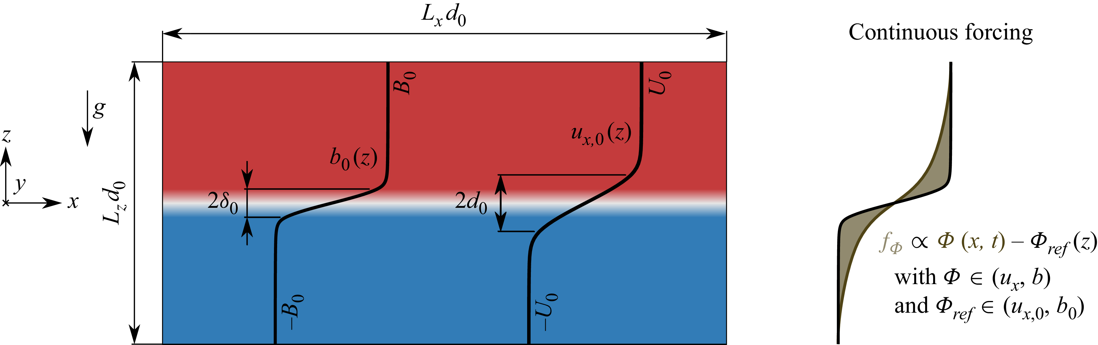


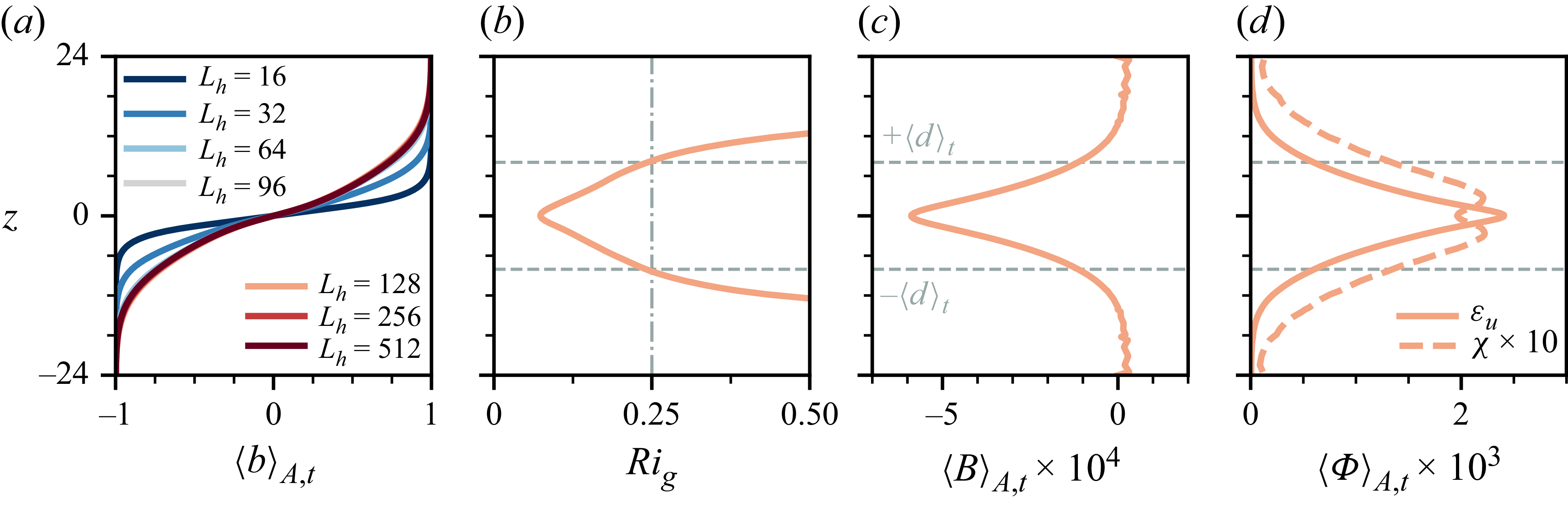


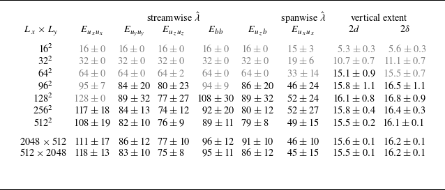


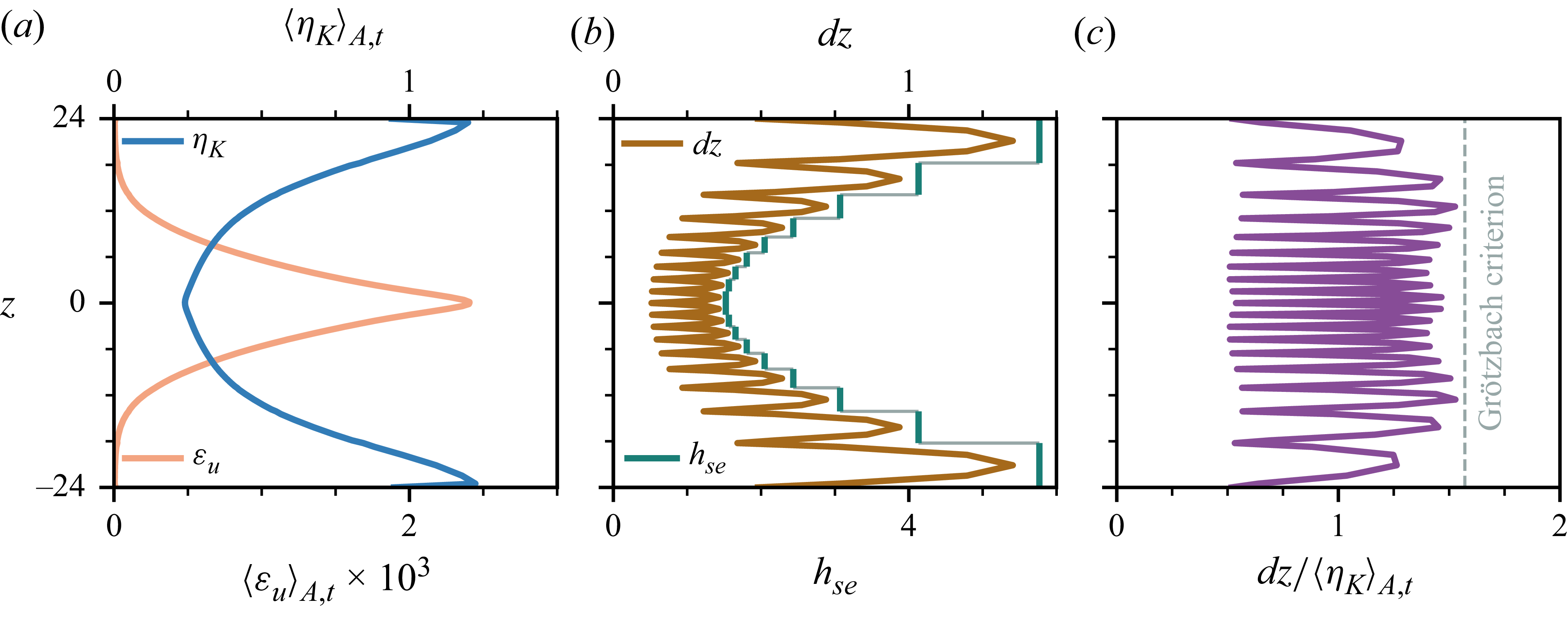


 Open access