


1. Introduction
Stellarators are again a subject of focus in nuclear fusion research. In particular, their inherent properties, namely steady-state operation and the absence of disruptions, are important requirements for a fusion power plant (Warmer et al. Reference Warmer2024). Ongoing optimisation of the magnetic field geometries leads to major improvements of their confinement properties. There are quasi-symmetric (QS) and quasi-isodynamic devices. Using magnetic coordinates (Boozer coordinates (Boozer Reference Boozer1982)), the magnetic field strength of QS stellarators is symmetric in the toroidal direction (quasi-axisymmetric (QA) (Nührenberg et al. Reference Nührenberg, Lotz and Gori1994; Henneberg et al. Reference Henneberg, Drevlak, Nührenberg, Beidler, Turkin, Loizu and Helander2019)), in the helical direction (quasi-helically symmetric (Nührenberg & Zille Reference Nührenberg and Zille1988)) or in the poloidal direction (quasi-poloidally symmetric (Spong et al. Reference Spong, Hirshman, Lyon, Berry and Strickler2005)). Quasi-isodynamic stellarators have no explicit symmetry, but their contours of the magnetic field strength are closed poloidally and the magnetic field is optimised to confine the trapped particles (Goodman et al. Reference Goodman, Camacho Mata, Henneberg, Jorge, Landreman, Plunk, Smith, Mackenbach, Beidler and Helander2023). However, due to their complex three-dimensional (3-D) geometry, the numerical description of stellarators is much more complicated than for axisymmetric tokamaks. While there are numerous numerical tools to investigate the linear stability properties of tokamaks (e.g. Mars-F (Liu et al. Reference Liu, Bondeson, Fransson, Lennartson and Breitholtz2000), MARS-K (Liu et al. Reference Liu, Chu, Chapman and Hender2008), MISHKA-F (Chapman et al. Reference Chapman, Sharapov, Huysmans and Mikhailovskii2006), MINERVA-DI (Aiba Reference Aiba2016) etc.), there exists only a limited number for stellarators (e.g. CAS3D (Nührenberg Reference Nührenberg2021) and TERPSICHORE (Anderson et al. Reference Anderson, Cooper, Gruber, Merazzi and Schwenn1990)). To our knowledge, the CASTOR3D code (Strumberger & Günter Reference Strumberger and Günter2017; Strumberger et al. Reference Strumberger, Günter, Lackner and Puchmayr2023) is the only 3-D linear stability code which includes simultaneously the effects of resistivity, parallel and gyro-viscosity, ion diamagnetic drift velocity, ExB velocity and externally driven flows.
The CASTOR3D code has already been successfully applied to external kink modes with low toroidal mode numbers in a QA stellarator configuration including parallel viscosity and toroidal flow (Strumberger & Günter Reference Strumberger and Günter2019) and to resistive internal kink and double tearing modes in Wendelstein 7-X (Strumberger et al. Reference Strumberger and Günter2020), and diamagnetic effects have been studied for ideal and resistive internal kink modes using simple axisymmetric and 3-D test equilibria (Strumberger et al. Reference Strumberger, Günter, Lackner and Puchmayr2023). CASTOR3D is also used for benchmarks with nonlinear extended magnetohydrodynamic (MHD) codes (e.g. JOREK (Nikulsin et al. Reference Nikulsin, Ramasamy, Hoelzl, Hindenlang, Strumberger, Lackner and Günter2022; Ramasamy et al. Reference Ramasamy, Aleynikova, Nikulsin, Hindenlang, Holod, Strumberger and Hoelzl2024) and NIMSTELL (Patil & Sovinec Reference Patil and Sovinec2024)). While former 3-D CASTOR3D stability calculations were restricted to low toroidal mode numbers, now also stability studies for peeling-ballooning modes in 3-D tokamak (Puchmayr et al. Reference Puchmayr2023, Reference Puchmayr, Dunne, Strumberger, Willensdorfer, Zohm and Hindenlang2024) and stellarator configurations are possible because of increasing memory and computing power, substantial improvement of the performance of the CASTOR3D code (Puchmayr Reference Puchmayr2023) and last but not least, the use of high fidelity equilibrium solutions computed with the GVEC code (Hindenlang et al. Reference Hindenlang, Babin, Maj, Ribeiro, Koeberl, Muir, Plunk and Sonnendrücker2025a ).
GVEC is a fixed-boundary 3-D MHD equilibrium solver that follows the same idea as VMEC (Hirshman & Whitson Reference Hirshman and Whitson1983), which is finding a set of nested flux surfaces via an energy minimisation. A distinct feature of GVEC is its radial discretisation with B-splines, thus providing a smooth high-order representation of the equilibrium solution, including the region around the magnetic axis. Furthermore, the coordinate frame to represent the flux surface geometry in GVEC is not restricted to cylindrical coordinates, which enables equilibrium solutions of highly shaped stellarator configurations (Hindenlang et al. Reference Hindenlang, Plunk and Maj2025b ). GVEC also provides the transformation into Boozer coordinates.
In the following, we present linear stability studies performed for a QA, high plasma- $\beta$
equilibrium which is unstable with respect to ideal external modes from low up to high toroidal mode numbers. This two-periodic stellarator equilibrium was already used for previous CASTOR3D stability studies described in detail in Strumberger & Günter (Reference Strumberger and Günter2019). Yet, at that time our computations were limited to
$\beta$
equilibrium which is unstable with respect to ideal external modes from low up to high toroidal mode numbers. This two-periodic stellarator equilibrium was already used for previous CASTOR3D stability studies described in detail in Strumberger & Günter (Reference Strumberger and Günter2019). Yet, at that time our computations were limited to $n_{tot}=7$
and
$n_{tot}=7$
and $m_{tot}=13$
per
$m_{tot}=13$
per $n$
, with
$n$
, with $n_{tot}$
and
$n_{tot}$
and $m_{tot}$
being the total numbers of toroidal and poloidal Fourier harmonics which could be used simultaneously. Therefore, we could only investigate external kink modes with low toroidal mode numbers taking into account parallel viscosity and toroidal flow. However, drift effects and the ExB velocity were not included in this older code version. We choose again this equilibrium because of its numerous and strong instabilities ranging from external kink to peeling-ballooning modes. We will study the effects of parallel viscosity, gyro-viscosity, ion diamagnetic drift velocity, ExB velocity and an externally driven flow in the direction of the quasi-symmetry with respect to their influence on the growth rate, oscillation frequency and mode structure of these external modes.
$m_{tot}$
being the total numbers of toroidal and poloidal Fourier harmonics which could be used simultaneously. Therefore, we could only investigate external kink modes with low toroidal mode numbers taking into account parallel viscosity and toroidal flow. However, drift effects and the ExB velocity were not included in this older code version. We choose again this equilibrium because of its numerous and strong instabilities ranging from external kink to peeling-ballooning modes. We will study the effects of parallel viscosity, gyro-viscosity, ion diamagnetic drift velocity, ExB velocity and an externally driven flow in the direction of the quasi-symmetry with respect to their influence on the growth rate, oscillation frequency and mode structure of these external modes.
In § 2, we present the linearised extended MHD equations which are used for the computations. The stability studies are the subject of § 3. We start with ideal stability studies in § 3.1. The effects of parallel viscosity and gyro-viscosity are discussed in § 3.2, while the effects of ion diamagnetic velocity, ExB velocity and an externally driven flow are investigated in § 3.3. In § 4, a summary of the results is given. Finally, the definition of the eigenfunctions and the determination of stellarator mode types is described in the appendix.
2. Linearised extended MHD equations
In this section, we briefly summarise the equations and definitions which are the basis of the presented stability studies. They are described in more detail in Strumberger et al. (Reference Strumberger, Günter, Lackner and Puchmayr2023).
The linearised extended MHD equations including parallel and gyro-viscosity, ion diamagnetic drift velocity, ExB velocity and additional poloidal and toroidal velocity terms read
 \begin{align} \lambda \rho _1 = -{\boldsymbol{V}}_0{\boldsymbol{\cdot}}{\boldsymbol{\nabla }} \rho _1- {\boldsymbol{V}}_1{\boldsymbol{\cdot}}{\boldsymbol{\nabla }} \rho _0 -\rho _1 {\boldsymbol{\nabla }}{\boldsymbol{\cdot}}{\boldsymbol{V}}_0 - \rho _0 {\boldsymbol{\nabla }}{\boldsymbol{\cdot}}{\boldsymbol{V}}_1, \end{align}
 \begin{align} \rho _0 \lambda {\boldsymbol{V}}_1 & = - \rho _1({\boldsymbol{V}}_0{\boldsymbol{\cdot}}{\boldsymbol{\nabla }}) {\boldsymbol{V}}_0 - \rho _0({\boldsymbol{V}}_1{\boldsymbol{\cdot}}{\boldsymbol{\nabla }}) {\boldsymbol{V}}_0 - \rho _0({\boldsymbol{V}}_0{\boldsymbol{\cdot}}{\boldsymbol{\nabla }}) {\boldsymbol{V}}_1 \nonumber \\[6pt] & \quad + \rho _1({\boldsymbol{V}}_{i0}^*{\boldsymbol{\cdot}}{\boldsymbol{\nabla }}) {\boldsymbol{V}}_0 + \rho _0({\boldsymbol{V}}_{i1}^*{\boldsymbol{\cdot}}{\boldsymbol{\nabla }}) {\boldsymbol{V}}_0 + \rho _0({\boldsymbol{V}}_{i0}^*{\boldsymbol{\cdot}}{\boldsymbol{\nabla }}) {\boldsymbol{V}}_1 \nonumber \\[5pt] & \quad - \frac {1}{m_i}{\boldsymbol{\nabla }}(\rho _0 T_1) - \frac {1}{m_i}{\boldsymbol{\nabla }}(T_0 \rho _1) +\mu _{||} \unicode{x1D6E5}_{||} {\boldsymbol{V}}_1 \nonumber \\[6pt] & \quad + \frac {1}{\mu _0} ({\boldsymbol{\nabla }} \times ({\boldsymbol{\nabla }} \times {\boldsymbol{A}}_1) ) \times ({\boldsymbol{\nabla }} \times {\boldsymbol{A}}_0) \nonumber \\[6pt] & \quad + \frac {1}{\mu _0} ({\boldsymbol{\nabla }} \times ({\boldsymbol{\nabla }} \times {\boldsymbol{A}}_0) ) \times ({\boldsymbol{\nabla }} \times {\boldsymbol{A}}_1), \end{align}
 \begin{align} \lambda T_1 = - {\boldsymbol{V}}_1{\boldsymbol{\cdot}}{\boldsymbol{\nabla }} T_0 - {\boldsymbol{V}}_0{\boldsymbol{\cdot}}{\boldsymbol{\nabla }} T_1 -(\varGamma -1) T_1 {\boldsymbol{\nabla }}{\boldsymbol{\cdot}}{\boldsymbol{V}}_0 -(\varGamma -1) T_0 {\boldsymbol{\nabla }}{\boldsymbol{\cdot}}{\boldsymbol{V}}_1, \end{align}
 \begin{align} \lambda {\boldsymbol{A}}_1={\boldsymbol{V}}_1 \times {\boldsymbol B}_0 + {\boldsymbol V_0} \times ({\boldsymbol{\nabla }} \times {\boldsymbol{A}}_1). \end{align}
Here, $\rho _0,{\boldsymbol{V}}_0, T_0,{\boldsymbol{A}}_0$
are the equilibrium quantities of density, velocity, temperature (
$\rho _0,{\boldsymbol{V}}_0, T_0,{\boldsymbol{A}}_0$
are the equilibrium quantities of density, velocity, temperature ( $T_0=T_{0e}+T_{0i}$
) and magnetic vector potential, while
$T_0=T_{0e}+T_{0i}$
) and magnetic vector potential, while $\rho _1,{\boldsymbol{V}}_1, T_1, {\boldsymbol{A}}_1$
are their perturbations. The perturbation of the ion diamagnetic drift velocity (2.6) reads
$\rho _1,{\boldsymbol{V}}_1, T_1, {\boldsymbol{A}}_1$
are their perturbations. The perturbation of the ion diamagnetic drift velocity (2.6) reads
 \begin{align} {\boldsymbol{V}}_{i1}^*&=-\alpha \alpha _T \frac {\rho _1}{\rho _0^2}\frac {{\boldsymbol B}_0 \times {\boldsymbol{\nabla }} p_0}{B_0^2}+\alpha \alpha _T \frac {1}{\rho _0} \frac {{\boldsymbol B}_0 \times (T_0 {\boldsymbol{\nabla }} \rho _1 + T_1 {\boldsymbol{\nabla }} \rho _0 +\rho _0 {\boldsymbol{\nabla }} T_1 +\rho _1 {\boldsymbol{\nabla }} T_0)}{B_0^2} \nonumber \\[5pt] & \quad +\alpha \alpha _T\frac {1}{\rho _0} \frac {({\boldsymbol{\nabla }} \times {\boldsymbol A_1}) \times {\boldsymbol{\nabla }} p_0}{B_0^2} -2\alpha \alpha _T\frac {1}{\rho _0} \frac {{\boldsymbol B}_0\boldsymbol{\cdot }({\boldsymbol{\nabla }} \times {\boldsymbol A_1})}{B_0^4}({\boldsymbol B}_0 \times {\boldsymbol{\nabla }} p_0). \end{align}
The time dependence of the perturbed quantities is taken to be ${\sim}e^{\lambda t}$
with eigenvalue
${\sim}e^{\lambda t}$
with eigenvalue $\lambda =\gamma +i \omega$
. The real part of
$\lambda =\gamma +i \omega$
. The real part of $\lambda$
corresponds to the growth rate
$\lambda$
corresponds to the growth rate $\gamma$
, while
$\gamma$
, while $\omega$
is the oscillation frequency of the perturbation.
$\omega$
is the oscillation frequency of the perturbation.
These equations correspond to the generally used linearised single-fluid equations (e.g. Huysmans, Goedbloed & Kerner Reference Huysmans, Goedbloed and Kerner1993) plus additional two-fluid terms. They are derived from the two-fluid MHD equations (Braginskii Reference Braginskii1965) making several assumptions and approximations, e.g. assuming quasi-neutrality $n=n_i=n_e$
(
$n=n_i=n_e$
( $n_i =$
ion density,
$n_i =$
ion density, $n_e =$
electron density), neglecting the electron mass
$n_e =$
electron density), neglecting the electron mass $m_e$
(
$m_e$
( $m_i \gt \gt m_e$
, mass density
$m_i \gt \gt m_e$
, mass density $\rho =m_i n+m_e n \approx m_i n$
) and using the pressure
$\rho =m_i n+m_e n \approx m_i n$
) and using the pressure $p=p_i+p_e=n(T_i+T_e)=nT$
(
$p=p_i+p_e=n(T_i+T_e)=nT$
( $T_i =$
ion temperature,
$T_i =$
ion temperature, $T_e =$
electron temperature). The unperturbed velocity
$T_e =$
electron temperature). The unperturbed velocity ${\boldsymbol{V}}_0$
corresponds to the ion velocity
${\boldsymbol{V}}_0$
corresponds to the ion velocity
 \begin{equation} {\boldsymbol{V}}_{0}={\boldsymbol{V}}_{i0} = \underbrace {\frac {{\boldsymbol E_0} \times {\boldsymbol B_0}}{B^2_0}}_{={\boldsymbol{V}}_{E\textrm {x}B}} + \underbrace {\alpha \frac {1}{\rho _0} \frac {{\boldsymbol B_0} \times {\boldsymbol{\nabla }} p_{i0}}{B^2_0}}_{={\boldsymbol{V}}_{i0}^*} + {\boldsymbol{V}}^{ext}. \end{equation}
Here, ${\boldsymbol{V}}_{E\textrm {x}B} + {\boldsymbol{V}}_{i0}^*$
are the ExB flow and the ion diamagnetic drift velocity with
${\boldsymbol{V}}_{E\textrm {x}B} + {\boldsymbol{V}}_{i0}^*$
are the ExB flow and the ion diamagnetic drift velocity with $\boldsymbol E_0$
and
$\boldsymbol E_0$
and $\boldsymbol B_0$
being the electric and magnetic fields, and
$\boldsymbol B_0$
being the electric and magnetic fields, and $\alpha = {m_i}/{e}$
with
$\alpha = {m_i}/{e}$
with $m_i$
and
$m_i$
and $e$
being the ion mass and elementary charge. Here, we neglect the parallel velocity, but we take into account an externally driven flow
$e$
being the ion mass and elementary charge. Here, we neglect the parallel velocity, but we take into account an externally driven flow ${\boldsymbol{V}}^{ext}$
, e.g. caused by neutral beam injection. Furthermore, the considered equations contain the linearised forms of the parallel viscous force density
${\boldsymbol{V}}^{ext}$
, e.g. caused by neutral beam injection. Furthermore, the considered equations contain the linearised forms of the parallel viscous force density $-{\boldsymbol{\nabla }}{\boldsymbol{\cdot}}{\varPi _{||}} = \mu _{||} \unicode{x1D6E5}_{||} {\boldsymbol{V}}$
Footnote
1
with
$-{\boldsymbol{\nabla }}{\boldsymbol{\cdot}}{\varPi _{||}} = \mu _{||} \unicode{x1D6E5}_{||} {\boldsymbol{V}}$
Footnote
1
with $\mu _{||}$
being the parallel viscosity coefficient, and the gyro-viscous force density being approximated by
$\mu _{||}$
being the parallel viscosity coefficient, and the gyro-viscous force density being approximated by $-{\boldsymbol{\nabla }}{\boldsymbol{\cdot}}{\varPi }_{\wedge }\approx \rho ({\boldsymbol{V}}^*_i{\boldsymbol{\cdot}}{\boldsymbol{\nabla }}) {\boldsymbol{V}}$
(Chang & Callen Reference Chang and Callen1992). Since, we consider single-fluid equations, but
$-{\boldsymbol{\nabla }}{\boldsymbol{\cdot}}{\varPi }_{\wedge }\approx \rho ({\boldsymbol{V}}^*_i{\boldsymbol{\cdot}}{\boldsymbol{\nabla }}) {\boldsymbol{V}}$
(Chang & Callen Reference Chang and Callen1992). Since, we consider single-fluid equations, but $T_i$
and
$T_i$
and $T_e$
may be different, we use
$T_e$
may be different, we use
 \begin{equation} T_i=\alpha _T T\,\,\,\,\,\textrm {and}\,\,\,\,\,T_e=(1-\alpha _T)T\,\,\,\,\,\textrm {with}\,\,\,\,\, 0\leqslant \alpha _T \leqslant 1. \end{equation}
The parameter $\alpha _T$
provides an additional degree of freedom that allows us to choose a more realistic ratio of ion and electron pressures with respect to the measured temperatures. The coefficients
$\alpha _T$
provides an additional degree of freedom that allows us to choose a more realistic ratio of ion and electron pressures with respect to the measured temperatures. The coefficients $\varGamma$
and
$\varGamma$
and $\mu_0$
denote the adiabtic index (
$\mu_0$
denote the adiabtic index ( $\varGamma=5/3$
) and the vacuum permeability.
$\varGamma=5/3$
) and the vacuum permeability.
3. Linear stability studies
As already mentioned, the two-periodic, QA equilibrium described in Strumberger & Günter (Reference Strumberger and Günter2019) is used for the following stability studies. Its high volume-averaged plasma beta of $\langle \beta \rangle =2.9\,\%$
together with the flat safety factor profile
$\langle \beta \rangle =2.9\,\%$
together with the flat safety factor profile $q(s)$
in the boundary region (boundary value
$q(s)$
in the boundary region (boundary value $q_b=1.79$
, see figure 1
b) make it unstable with respect to ideal external kink and peeling-ballooning modes. Since, highly accurate equilibria are the basis for the ambitious stability studies presented below, we recalculated the equilibrium with the 3-D equilibrium code GVEC (Hindenlang et al. Reference Hindenlang, Babin, Maj, Ribeiro, Koeberl, Muir, Plunk and Sonnendrücker2025a
) and used its transformation into Boozer coordinates. For the equilibrium calculation with GVEC, we used
$q_b=1.79$
, see figure 1
b) make it unstable with respect to ideal external kink and peeling-ballooning modes. Since, highly accurate equilibria are the basis for the ambitious stability studies presented below, we recalculated the equilibrium with the 3-D equilibrium code GVEC (Hindenlang et al. Reference Hindenlang, Babin, Maj, Ribeiro, Koeberl, Muir, Plunk and Sonnendrücker2025a
) and used its transformation into Boozer coordinates. For the equilibrium calculation with GVEC, we used $20$
toroidal and
$20$
toroidal and $18$
poloidal Fourier harmonics and
$18$
poloidal Fourier harmonics and $300$
radial elements with a polynomial degree of the radial B-splines of
$300$
radial elements with a polynomial degree of the radial B-splines of $5$
. The transformation into Boozer coordinates has been calculated with GVEC using
$5$
. The transformation into Boozer coordinates has been calculated with GVEC using $80$
toroidal and
$80$
toroidal and $72$
poloidal Fourier harmonics in the new Boozer coordinate system. While we simply used a constant density in the previous stability studies, we now use a density profile (
$72$
poloidal Fourier harmonics in the new Boozer coordinate system. While we simply used a constant density in the previous stability studies, we now use a density profile ( $\rho _0 = m_i n_a (1-0.8 s^4)$
,
$\rho _0 = m_i n_a (1-0.8 s^4)$
, $n_a=4 \times 10^{19}\,{\textrm {m}}^{-3}$
,
$n_a=4 \times 10^{19}\,{\textrm {m}}^{-3}$
, $m_i =$
deuteron mass). The latter leads to higher growth rates because of the reduced inertia in the boundary region. Figure 1(c) shows the normalised profiles of density and temperature.
$m_i =$
deuteron mass). The latter leads to higher growth rates because of the reduced inertia in the boundary region. Figure 1(c) shows the normalised profiles of density and temperature.

Figure 1. (a) Poloidal and toroidal coordinate lines in Boozer coordinates at the plasma boundary ( $s = 1$
) of the QA equilibrium. (b) Safety factor, (c) normalised density and temperature profiles, (d) toroidal and (e) poloidal ion drift frequencies (3.2) as functions of the square root of the normalised toroidal flux
$s = 1$
) of the QA equilibrium. (b) Safety factor, (c) normalised density and temperature profiles, (d) toroidal and (e) poloidal ion drift frequencies (3.2) as functions of the square root of the normalised toroidal flux $s$
.
$s$
.

Boozer magnetic flux coordinates ( $s,v,u$
) are advantageous for 3-D stability studies because magnetic field lines are straight in these coordinates (Boozer Reference Boozer1982). Figure 1(a) illustrates the toroidal
$s,v,u$
) are advantageous for 3-D stability studies because magnetic field lines are straight in these coordinates (Boozer Reference Boozer1982). Figure 1(a) illustrates the toroidal $v$
and poloidal
$v$
and poloidal $u$
coordinate lines at the plasma boundary of the QA equilibrium while the square root of the normalised toroidal flux serves as the radial coordinate
$u$
coordinate lines at the plasma boundary of the QA equilibrium while the square root of the normalised toroidal flux serves as the radial coordinate $s$
. Using these coordinates, the ion diamagnetic drift velocity reads
$s$
. Using these coordinates, the ion diamagnetic drift velocity reads
 \begin{align*} {\boldsymbol{V}}_{i0}^*=\frac {m_i}{e}\frac {1}{\rho _0} \frac {{\boldsymbol B_0} \times \boldsymbol{\nabla }p_{i0}}{B_0^2}\end{align*}
 \begin{align} =\frac {m_i}{e}\frac {1}{\rho _0}\frac {\partial p_{i0}}{\partial s} \left (\frac {I}{\varPhi 'J+\varPsi 'I}{\boldsymbol r}_{,v} - \frac {J}{\varPhi 'J+\varPsi 'I}\boldsymbol {r}_{,u}\right ) = \frac {1}{2\pi } \varOmega _{tor}^{i*} {\boldsymbol r}_{,v} + \frac {1}{2\pi } \varOmega _{pol}^{i*} {\boldsymbol r}_{,u} ,\end{align}
with
 \begin{equation} \varOmega _{tor}^{i*}(s)=2\pi \frac {m_i}{e}\frac {1}{\rho _0}\frac {\partial p_{i0}}{\partial s} \frac {I}{\varPhi 'J+\varPsi 'I}\,\,\,\,\,\textrm {and}\,\,\,\,\, \varOmega _{pol}^{i*}(s)=-2\pi \frac {m_i}{e}\frac {1}{\rho _0}\frac {\partial p_{i0}}{\partial s} \frac {J}{\varPhi 'J+\varPsi 'I} \end{equation}
being constant on flux surfaces. Here, $I(s)$
and
$I(s)$
and $J(s)$
are the total toroidal and poloidal currents, while
$J(s)$
are the total toroidal and poloidal currents, while $\varPhi '$
and
$\varPhi '$
and $\varPsi '$
are the derivatives of the toroidal
$\varPsi '$
are the derivatives of the toroidal $\varPhi (s)$
and poloidal
$\varPhi (s)$
and poloidal $\varPsi (s)$
fluxes. The toroidal
$\varPsi (s)$
fluxes. The toroidal $\varOmega _{tor}^{i*}(s)$
and poloidal
$\varOmega _{tor}^{i*}(s)$
and poloidal $\varOmega _{pol}^{i*}(s)$
drift frequencies are shown in figures 1(d) and 1(e). As expected, the poloidal frequency is much larger than the toroidal one (
$\varOmega _{pol}^{i*}(s)$
drift frequencies are shown in figures 1(d) and 1(e). As expected, the poloidal frequency is much larger than the toroidal one ( $J \gg I$
).
$J \gg I$
).
We implemented the ExB velocity in the CASTOR3D code assuming that the electric potential $\varPhi _E$
is constant on flux surfaces, that is,
$\varPhi _E$
is constant on flux surfaces, that is,
 \begin{equation} {\boldsymbol E_0}= -\frac {\partial \varPhi _E}{\partial s} \boldsymbol{\nabla }s = E_s \boldsymbol{\nabla }s, \end{equation}
with $E_s$
being the radial co-variant component. This assumption excludes radial flows which would be generated by non-radial components of
$E_s$
being the radial co-variant component. This assumption excludes radial flows which would be generated by non-radial components of $\boldsymbol{E}_0$
. Analogous to the ion diamagnetic drift velocity (3.1), we obtain in Boozer coordinates
$\boldsymbol{E}_0$
. Analogous to the ion diamagnetic drift velocity (3.1), we obtain in Boozer coordinates
 \begin{equation} {\boldsymbol{V}}_{ExB}=\frac {{\boldsymbol B_0} \times \boldsymbol{\nabla }{\varPhi _E(s)}}{{B_0^2}}= \frac {1}{2\pi } \varOmega _{tor}^{ExB} {\boldsymbol r}_{,v} + \frac {1}{2\pi } \varOmega _{pol}^{ExB} {\boldsymbol r}_{,u}. \end{equation}
Assuming $T_{i0} \approx T_{e0}$
, that is,
$T_{i0} \approx T_{e0}$
, that is, $\alpha _T=0.5$
(2.7) and
$\alpha _T=0.5$
(2.7) and $\hat \nu _i /\sqrt {m_i} \approx \hat \nu _e /\sqrt {m_e}$
(
$\hat \nu _i /\sqrt {m_i} \approx \hat \nu _e /\sqrt {m_e}$
( $\hat \nu _i$
and
$\hat \nu _i$
and $\hat \nu _e$
are the ion and electron collision frequencies normalised to the corresponding particle masses with
$\hat \nu _e$
are the ion and electron collision frequencies normalised to the corresponding particle masses with $m_i \ll m_e$
), the well-known ambipolarity condition (Stroth, Manz & Ramisch Reference Stroth, Manz and Ramisch2011; Viezzer Reference Viezzer2012) simplifies to
$m_i \ll m_e$
), the well-known ambipolarity condition (Stroth, Manz & Ramisch Reference Stroth, Manz and Ramisch2011; Viezzer Reference Viezzer2012) simplifies to
 \begin{equation} E_s \approx \frac {m_i}{e}\frac {1}{\rho _0}\frac {\partial p_{i0}}{\partial s}, \end{equation}
represented by the black curve in figure 2(a). In this case, the ion diamagnetic drift velocity is balanced by the ExB velocity. The red curve shows a hypothetical profile of $E_s$
which, in combination with the ion diamagnetic drift velocity, leads to a finite velocity. Usually,
$E_s$
which, in combination with the ion diamagnetic drift velocity, leads to a finite velocity. Usually, $E_s$
will be provided by experimental measurements, however, such a profile is not available for our quasi-axisymmetric test equilibrium. Figures 2(b) and 2(c) show the corresponding toroidal and poloidal frequency profiles of the ExB velocity obtained from the two types of
$E_s$
will be provided by experimental measurements, however, such a profile is not available for our quasi-axisymmetric test equilibrium. Figures 2(b) and 2(c) show the corresponding toroidal and poloidal frequency profiles of the ExB velocity obtained from the two types of $E_s$
presented in figure 2(a). Again, the poloidal frequency is much larger than the toroidal one because
$E_s$
presented in figure 2(a). Again, the poloidal frequency is much larger than the toroidal one because $J\gg I$
. However, analogous to a tokamak, a plasma of a QA stellarator enjoys ‘intrinsic ambipolarity’ and is free to rotate in the direction of symmetry (Helander & Simakov Reference Helander and Simakov2008) which corresponds to the toroidal direction (
$J\gg I$
. However, analogous to a tokamak, a plasma of a QA stellarator enjoys ‘intrinsic ambipolarity’ and is free to rotate in the direction of symmetry (Helander & Simakov Reference Helander and Simakov2008) which corresponds to the toroidal direction ( $v$
-direction) in Boozer coordinates. That is, neutral beam injection, lower hybrid waves, etc. may drive a fast toroidal rotation. We use a hypothetical toroidal rotation profile with
$v$
-direction) in Boozer coordinates. That is, neutral beam injection, lower hybrid waves, etc. may drive a fast toroidal rotation. We use a hypothetical toroidal rotation profile with $\varOmega _{tor}^{ext}=\varOmega _0(1-0.8s^4)$
to study the combined effects of parallel viscosity, gyro-viscosity, the velocities
$\varOmega _{tor}^{ext}=\varOmega _0(1-0.8s^4)$
to study the combined effects of parallel viscosity, gyro-viscosity, the velocities ${\boldsymbol{V}}_{i0}^*$
and
${\boldsymbol{V}}_{i0}^*$
and ${\boldsymbol{V}}_{ExB}$
and an externally driven toroidal flow
${\boldsymbol{V}}_{ExB}$
and an externally driven toroidal flow ${\boldsymbol{V}}^{ext}= ({1}/{2\pi })\varOmega _{tor}^{ext}{\boldsymbol r},_v$
in § 3.3.
${\boldsymbol{V}}^{ext}= ({1}/{2\pi })\varOmega _{tor}^{ext}{\boldsymbol r},_v$
in § 3.3.

Figure 3. (a) Growth rate as function of the dominating toroidal mode number $n^*$
for an ideal equilibrium. The results are subdivided into odd (black and green) and even (red and blue) mode families, and into full- (black and red) and reduced-size (green and blue) calculations. The results of the full-size calculations are marked by circles (sine-type solutions) and plus symbols (cosine-type solutions). (b)–(e) Eigenfunction Fourier spectra of the radial velocity perturbation for (b) sine-type and (c) cosine-type
$n^*$
for an ideal equilibrium. The results are subdivided into odd (black and green) and even (red and blue) mode families, and into full- (black and red) and reduced-size (green and blue) calculations. The results of the full-size calculations are marked by circles (sine-type solutions) and plus symbols (cosine-type solutions). (b)–(e) Eigenfunction Fourier spectra of the radial velocity perturbation for (b) sine-type and (c) cosine-type $n^* = 4$
external kink modes, (d) a cosine-type
$n^* = 4$
external kink modes, (d) a cosine-type $n^* = 19$
and (e) an
$n^* = 19$
and (e) an $n^* = 44$
peeling-ballooning mode. The latter has been computed using the reduced-size eigenvalue problem.
$n^* = 44$
peeling-ballooning mode. The latter has been computed using the reduced-size eigenvalue problem.
3.1. Ideal external modes
We start the stability studies with the pure ideal MHD equations, that is, without taking viscosity, drift effects or plasma flow into account. While modes of axisymmetric tokamak equilibria are characterised by their toroidal mode number $n$
, several toroidal harmonics couple in the case of a 3-D plasma configuration. We, therefore, introduced the toroidal mode number
$n$
, several toroidal harmonics couple in the case of a 3-D plasma configuration. We, therefore, introduced the toroidal mode number $n^*$
(Strumberger & Günter Reference Strumberger and Günter2019) to characterise the modes, with
$n^*$
(Strumberger & Günter Reference Strumberger and Günter2019) to characterise the modes, with $n^*$
being the dominant toroidal harmonic contributing to the Fourier spectrum of the mode. While in the case of low-
$n^*$
being the dominant toroidal harmonic contributing to the Fourier spectrum of the mode. While in the case of low- $n^*$
modes
$n^*$
modes $n^*$
can be easily identified by regarding the Fourier spectra of the eigenfunctions (figures 3
b and 3
c), this method becomes very difficult (figure 3
d) or even impossible for high-
$n^*$
can be easily identified by regarding the Fourier spectra of the eigenfunctions (figures 3
b and 3
c), this method becomes very difficult (figure 3
d) or even impossible for high- $n^*$
modes (figure 3
e). For this reason, we compute the contributions of the Fourier harmonics in dependence on
$n^*$
modes (figure 3
e). For this reason, we compute the contributions of the Fourier harmonics in dependence on $n$
and then determine the
$n$
and then determine the $n$
value with the maximum contribution (for details see appendix, equations (A5) and (A6)). Yet, even this method does not always yield distinct results, as shown in the subsequent sections.
$n$
value with the maximum contribution (for details see appendix, equations (A5) and (A6)). Yet, even this method does not always yield distinct results, as shown in the subsequent sections.
Figure 3(a) presents the growth rates $\gamma$
of ideal external modes as functions of
$\gamma$
of ideal external modes as functions of $n^*$
. The fluctuations of
$n^*$
. The fluctuations of $\gamma$
result from the varying distances of the mode relevant rational surfaces from the plasma boundary. These fluctuations are largest for small
$\gamma$
result from the varying distances of the mode relevant rational surfaces from the plasma boundary. These fluctuations are largest for small $n^*$
and decrease with increasing mode number. Disregarding the fluctuations, the growth rates increase with rising
$n^*$
and decrease with increasing mode number. Disregarding the fluctuations, the growth rates increase with rising $n^*$
, that is, the high-
$n^*$
, that is, the high- $n^*$
peeling-ballooning modes are more unstable than the low-
$n^*$
peeling-ballooning modes are more unstable than the low- $n^*$
external kink modes. Because of the two-periodic geometry of the equilibrium, there exist two mode families, namely the so-called odd (n = 1,3,5,…) and even (n = 0,2,4,6,…) mode families. Only the harmonics of a mode family couple together (Nührenberg Reference Nührenberg1996). The eigenfunctions (A1) couple to pure sine- and cosine-type functions with specific locations because of the stellarator symmetry of the QA equilibrium. Figures 3(b) and 3(c) show the Fourier coefficients of the radial velocity perturbation as functions of s (A4) for the
$n^*$
external kink modes. Because of the two-periodic geometry of the equilibrium, there exist two mode families, namely the so-called odd (n = 1,3,5,…) and even (n = 0,2,4,6,…) mode families. Only the harmonics of a mode family couple together (Nührenberg Reference Nührenberg1996). The eigenfunctions (A1) couple to pure sine- and cosine-type functions with specific locations because of the stellarator symmetry of the QA equilibrium. Figures 3(b) and 3(c) show the Fourier coefficients of the radial velocity perturbation as functions of s (A4) for the $n^*=4$
external kink modes. Here,
$n^*=4$
external kink modes. Here, $\hat v^s_{mn}$
and
$\hat v^s_{mn}$
and $\hat {\bar v}^s_{mn}$
are exactly equal with opposite (sine-type) and equal signs (cosine-type), respectively. This holds for both the real and (not shown) imaginary parts, while the signs and amplitudes of real and imaginary parts may be different (see appendix). The growth rates of the two modes are slightly different, that is, one location promotes the growth of the mode more than the other. Here, growth rates of sine- and cosine-type modes are clearly non-degenerate for
$\hat {\bar v}^s_{mn}$
are exactly equal with opposite (sine-type) and equal signs (cosine-type), respectively. This holds for both the real and (not shown) imaginary parts, while the signs and amplitudes of real and imaginary parts may be different (see appendix). The growth rates of the two modes are slightly different, that is, one location promotes the growth of the mode more than the other. Here, growth rates of sine- and cosine-type modes are clearly non-degenerate for $n^* \leqslant 6$
with
$n^* \leqslant 6$
with $|\unicode{x1D6E5} \gamma | \geqslant 1$
%. These modes are locked to their positions, that is, plasma flow has to exceed a critical value to unlock them. The critical value decreases with
$|\unicode{x1D6E5} \gamma | \geqslant 1$
%. These modes are locked to their positions, that is, plasma flow has to exceed a critical value to unlock them. The critical value decreases with $\unicode{x1D6E5} \gamma$
and becomes zero for degenerate growth rates (Strumberger & Günter Reference Strumberger and Günter2019; Puchmayr et al. Reference Puchmayr2023).
$\unicode{x1D6E5} \gamma$
and becomes zero for degenerate growth rates (Strumberger & Günter Reference Strumberger and Günter2019; Puchmayr et al. Reference Puchmayr2023).
Even in cases where the growth rates are equal within the numerical accuracy, the stellarator symmetry leads to sine- and cosine-type eigenfunctions, as shown for a cosine-type $n^* = 19$
mode in figure 3(d). The ideal 3-D CAS3D code is able to exploit the stellarator symmetry and to separate the eigenvalue problem into sine- and cosine-type solutions (Nührenberg Reference Nührenberg1996, Reference Nührenberg2016), while the CASTOR3D code solves a complex eigenvalue problem based on complex and complex-conjugate exponential functions (A1). However, when the coupling between the two parts no longer plays a role, which implies that the growth rates are degenerate, the ansatz for the eigenfunctions (A1) and with it the size of the eigenvalue problem can be reduced considerably by neglecting the complex-conjugate exponential function part (A3). The reduction of the matrix size by a factor of four leads to an important reduction of memory and computational time, so that the number of included poloidal and toroidal harmonics and/or the number of radial grid points can be increased accordingly. This increase is essential to achieve a sufficient numerical accuracy for the computation of high-
$n^* = 19$
mode in figure 3(d). The ideal 3-D CAS3D code is able to exploit the stellarator symmetry and to separate the eigenvalue problem into sine- and cosine-type solutions (Nührenberg Reference Nührenberg1996, Reference Nührenberg2016), while the CASTOR3D code solves a complex eigenvalue problem based on complex and complex-conjugate exponential functions (A1). However, when the coupling between the two parts no longer plays a role, which implies that the growth rates are degenerate, the ansatz for the eigenfunctions (A1) and with it the size of the eigenvalue problem can be reduced considerably by neglecting the complex-conjugate exponential function part (A3). The reduction of the matrix size by a factor of four leads to an important reduction of memory and computational time, so that the number of included poloidal and toroidal harmonics and/or the number of radial grid points can be increased accordingly. This increase is essential to achieve a sufficient numerical accuracy for the computation of high- $n^*$
peeling-ballooning modes. Performing the full- and the reduced-size eigenvalue problems under the same conditions for intermediate
$n^*$
peeling-ballooning modes. Performing the full- and the reduced-size eigenvalue problems under the same conditions for intermediate $n^*$
-values, we obtain the same eigenvalues as shown in figure 3(a). Figure 3(e) shows the Fourier spectrum of the radial velocity perturbation of an
$n^*$
-values, we obtain the same eigenvalues as shown in figure 3(a). Figure 3(e) shows the Fourier spectrum of the radial velocity perturbation of an $n^* = 44$
peeling-ballooning mode computed with the reduced-size eigenvalue problem.
$n^* = 44$
peeling-ballooning mode computed with the reduced-size eigenvalue problem.
3.2. Parallel and gyro-viscosity
In a first step, we consider only the parallel viscosity. Using a rough estimate of the parallel viscosity coefficientFootnote
2
(Strumberger & Günter Reference Strumberger and Günter2019), we get $1 \lesssim \mu _{||} \lesssim 10$
kg ms−1.
$1 \lesssim \mu _{||} \lesssim 10$
kg ms−1.

Figure 4. (a) Contributions of the toroidal Fourier harmonics ( $f_{RE}$
(solid lines),
$f_{RE}$
(solid lines), $\bar f_{RE}$
(symbols)) to the
$\bar f_{RE}$
(symbols)) to the $n^* = 1/n^* = 5$
cosine-type mode for various values of the parallel viscosity coefficient
$n^* = 1/n^* = 5$
cosine-type mode for various values of the parallel viscosity coefficient $\mu _{||}$
. (b) Growth rates as functions of
$\mu _{||}$
. (b) Growth rates as functions of $n^*$
without (black circles) and with (red circles) taking parallel viscosity into account. (c) Growth rates as functions of the dynamic viscosity coefficient
$n^*$
without (black circles) and with (red circles) taking parallel viscosity into account. (c) Growth rates as functions of the dynamic viscosity coefficient $\mu _{||}$
for
$\mu _{||}$
for $n^* = 1$
and
$n^* = 1$
and $n^* = 9$
sine-type (circles) and cosine-type (plus symbols) modes. (d) Oscillation frequencies of the sine-type and cosine-type
$n^* = 9$
sine-type (circles) and cosine-type (plus symbols) modes. (d) Oscillation frequencies of the sine-type and cosine-type $n^* = 1 \leftrightarrow n^* = 9$
overstable modes. (e) Real and (f) imaginary parts of the eigenfunction Fourier spectrum for the radial velocity perturbation of the sine-type overstable mode (
$n^* = 1 \leftrightarrow n^* = 9$
overstable modes. (e) Real and (f) imaginary parts of the eigenfunction Fourier spectrum for the radial velocity perturbation of the sine-type overstable mode ( $\mu _{||} = 1.1$
kg ms−1).
$\mu _{||} = 1.1$
kg ms−1).
In figure 3(a), which shows the ideal growth rates without viscosity, there are growth rates for two cosine-type $n^* = 5$
modes, while the value of the cosine-type
$n^* = 5$
modes, while the value of the cosine-type $n^* = 1$
mode is missing. Comparing, on the contrary, the growth rates of the
$n^* = 1$
mode is missing. Comparing, on the contrary, the growth rates of the $n^* = 1$
and the
$n^* = 1$
and the $n^* = 5$
modes, it seems reasonable to assign the more unstable cosine-type
$n^* = 5$
modes, it seems reasonable to assign the more unstable cosine-type $n^* = 5$
mode to the sine-type
$n^* = 5$
mode to the sine-type $n^* = 1$
mode. Turning on the parallel viscosity confirms that this assignment is justified. Figure 4(a) presents the normalised functions
$n^* = 1$
mode. Turning on the parallel viscosity confirms that this assignment is justified. Figure 4(a) presents the normalised functions $f_{{Re}}(n)$
and
$f_{{Re}}(n)$
and $\bar f_{{Re}}(n)$
(A5) for various parallel viscosity coefficients
$\bar f_{{Re}}(n)$
(A5) for various parallel viscosity coefficients $\mu _{||}$
. As explained in the appendix, the maxima of these functions define the most contributing toroidal Fourier harmonic
$\mu _{||}$
. As explained in the appendix, the maxima of these functions define the most contributing toroidal Fourier harmonic $n^*$
. This maximum value changes from
$n^*$
. This maximum value changes from $n^* = 5$
to
$n^* = 5$
to $n^* = 1$
in the range of
$n^* = 1$
in the range of $2 \lt \mu _{||} \lt 3$
kg ms−1. That is, the parallel viscosity has not only a stabilising effect, as shown in figure 4(b), but it can also change the structure of the mode and its
$2 \lt \mu _{||} \lt 3$
kg ms−1. That is, the parallel viscosity has not only a stabilising effect, as shown in figure 4(b), but it can also change the structure of the mode and its $n^*$
-type. Nevertheless, the modes are still sine- and cosine-type modes, respectively.
$n^*$
-type. Nevertheless, the modes are still sine- and cosine-type modes, respectively.
The growth rates of external kink and peeling-ballooning modes with and without parallel viscosity are compared in figure 4(b). The damping effect of the parallel viscosity increases with $n^*$
. The peeling-ballooning modes are clearly less unstable if a viscosity of
$n^*$
. The peeling-ballooning modes are clearly less unstable if a viscosity of $\mu _{||}=4$
kg ms−1 is included. Yet, the high-
$\mu _{||}=4$
kg ms−1 is included. Yet, the high- $n^*$
peeling-ballooning modes are still more unstable than the low-
$n^*$
peeling-ballooning modes are still more unstable than the low- $n^*$
external kink modes.
$n^*$
external kink modes.
Since the damping of the growth rate depends on the mode type, the lines representing the growth rates of the sine- and cosine-type $n^* = 9$
modes intersect the lines of the
$n^* = 9$
modes intersect the lines of the $n^* = 1$
modes in figure 4(c). In these intersection regions the sine-type
$n^* = 1$
modes in figure 4(c). In these intersection regions the sine-type $n^* = 1$
and
$n^* = 1$
and $n^* = 9$
modes (
$n^* = 9$
modes ( $1\lt \mu _{||} \lt 1.3$
kg ms−1) and the cosine-type
$1\lt \mu _{||} \lt 1.3$
kg ms−1) and the cosine-type $n^* = 1$
and
$n^* = 1$
and $n^* = 9$
modes (
$n^* = 9$
modes ( $3.4\lt \mu _{||} \lt 4.1$
kg ms−1) couple to oscillating overstable modes which oscillate between the
$3.4\lt \mu _{||} \lt 4.1$
kg ms−1) couple to oscillating overstable modes which oscillate between the $n^* = 1$
and
$n^* = 1$
and $n^* = 9$
types, as figures 4(e) and 4(f) illustrate. Here, the real and the imaginary parts of the eigenfunction Fourier spectrum are presented for the radial velocity perturbation of the sine-type overstable mode. The real part corresponds to the
$n^* = 9$
types, as figures 4(e) and 4(f) illustrate. Here, the real and the imaginary parts of the eigenfunction Fourier spectrum are presented for the radial velocity perturbation of the sine-type overstable mode. The real part corresponds to the $n^* = 9$
mode, while the imaginary part represents the
$n^* = 9$
mode, while the imaginary part represents the $n^* = 1$
mode. The resulting perturbation multiplied with the eigenvalue describes a growing mode oscillating between the
$n^* = 1$
mode. The resulting perturbation multiplied with the eigenvalue describes a growing mode oscillating between the $n^* = 9$
and
$n^* = 9$
and $n^* = 1$
state. The oscillation frequencies of the overstable modes are illustrated in figure 4(d). In axisymmetric equilibria an overstable mode may occur if at least two unstable modes of the same
$n^* = 1$
state. The oscillation frequencies of the overstable modes are illustrated in figure 4(d). In axisymmetric equilibria an overstable mode may occur if at least two unstable modes of the same $n$
-type exist and their growth rates overlap within certain ranges of plasma parameters. When the growth rates as functions of a single parameter (e.g. pressure gradient (Kerner, Jakoby & Lerbinger Reference Kerner, Jakoby and Lerbinger1986), resistivity (Huysmans et al. Reference Huysmans, Goedbloed and Kerner1993), etc.) become the same, an overstable oscillating mode evolves. However, the toroidal harmonics are coupled in 3-D equilibria. Therefore, overstable modes can also evolve if the growth rates of any
$n$
-type exist and their growth rates overlap within certain ranges of plasma parameters. When the growth rates as functions of a single parameter (e.g. pressure gradient (Kerner, Jakoby & Lerbinger Reference Kerner, Jakoby and Lerbinger1986), resistivity (Huysmans et al. Reference Huysmans, Goedbloed and Kerner1993), etc.) become the same, an overstable oscillating mode evolves. However, the toroidal harmonics are coupled in 3-D equilibria. Therefore, overstable modes can also evolve if the growth rates of any $n^*$
-modes of the same mode family overlap within a certain parameter range (Strumberger et al. Reference Strumberger and Günter2020). The occurrence of overstable modes strongly depends on the equilibrium parameters (Kerner et al. Reference Kerner, Jakoby and Lerbinger1986). Our computations confirm that the effect disappears for slightly different parameters.
$n^*$
-modes of the same mode family overlap within a certain parameter range (Strumberger et al. Reference Strumberger and Günter2020). The occurrence of overstable modes strongly depends on the equilibrium parameters (Kerner et al. Reference Kerner, Jakoby and Lerbinger1986). Our computations confirm that the effect disappears for slightly different parameters.
Assuming that there is no external flow drive and that the ambipolarity condition (3.5) holds ( ${\boldsymbol{V}}_{ExB}=-{\boldsymbol{V}}_{i0}^*$
), all terms containing
${\boldsymbol{V}}_{ExB}=-{\boldsymbol{V}}_{i0}^*$
), all terms containing ${\boldsymbol{V}}_0$
disappear in the linearised MHD equations (2.1)–(2.4), and the linearised momentum equation (2.2) reads
${\boldsymbol{V}}_0$
disappear in the linearised MHD equations (2.1)–(2.4), and the linearised momentum equation (2.2) reads
 \begin{align} \rho _0 \lambda {\boldsymbol{V}}_1 & = - \frac {1}{m_i}{\boldsymbol{\nabla }}(\rho _0 T_1) - \frac {1}{m_i}{\boldsymbol{\nabla }}(T_0 \rho _1) + \rho _0({\boldsymbol{V}}_{i0}^*{\boldsymbol{\cdot}}{\boldsymbol{\nabla }}) {\boldsymbol{V}}_1 +\mu _{||} \unicode{x1D6E5}_{||} {\boldsymbol{V}}_1\nonumber \\[5pt] & \quad + \frac {1}{\mu _0} ({\boldsymbol{\nabla }} \times ({\boldsymbol{\nabla }} \times {\boldsymbol{A}}_1) ) \times ({\boldsymbol{\nabla }} \times {\boldsymbol{A}}_0) + \frac {1}{\mu _0} ({\boldsymbol{\nabla }} \times ({\boldsymbol{\nabla }} \times {\boldsymbol{A}}_0) ) \times ({\boldsymbol{\nabla }} \times {\boldsymbol{A}}_1). \end{align}
While the parallel viscosity only reduces the growth rate, but does not cause mode oscillations,Footnote
3
the gyro-viscosity term leads to oscillations. Assuming a parallel viscosity of $\mu _{||}=4$
kg ms−1, the gyro-viscosity decouples the
$\mu _{||}=4$
kg ms−1, the gyro-viscosity decouples the $n^* = 1$
,
$n^* = 1$
, $n^* = 9$
cosine-type overstable mode already if only
$n^* = 9$
cosine-type overstable mode already if only $\approx$
1 % of its nominal amplitude is taken into account (
$\approx$
1 % of its nominal amplitude is taken into account ( $\alpha _s \gt 0.01$
).Footnote
4
The remaining
$\alpha _s \gt 0.01$
).Footnote
4
The remaining $n^* = 1$
cosine-type mode stops oscillation, while the growth rates of the cosine- and sine-type
$n^* = 1$
cosine-type mode stops oscillation, while the growth rates of the cosine- and sine-type $n^* = 9$
become equal and start to oscillate in the range of
$n^* = 9$
become equal and start to oscillate in the range of $0.05 \lt \alpha _s \lt 0.075$
. However, even the full gyro-viscosity term (
$0.05 \lt \alpha _s \lt 0.075$
. However, even the full gyro-viscosity term ( $\alpha _s = 1$
) is not strong enough to unlock the
$\alpha _s = 1$
) is not strong enough to unlock the $n^* = 1$
modes of the considered plasma configuration, whereas all instabilities with
$n^* = 1$
modes of the considered plasma configuration, whereas all instabilities with $n^* \gt 1$
unlock and oscillate. As an example, figures 5(a) and 5(b) show the behaviour of the
$n^* \gt 1$
unlock and oscillate. As an example, figures 5(a) and 5(b) show the behaviour of the $n^* = 2$
modes as a function of
$n^* = 2$
modes as a function of $\alpha _s$
. The initially non-degenerate growth rates converge until they become equal for
$\alpha _s$
. The initially non-degenerate growth rates converge until they become equal for $\alpha _s \lesssim 0.77$
. At that point the modes unlock and start to oscillate. Figure 5(c) illustrates the growth rates and oscillation frequencies as functions of
$\alpha _s \lesssim 0.77$
. At that point the modes unlock and start to oscillate. Figure 5(c) illustrates the growth rates and oscillation frequencies as functions of $n^*$
if parallel and gyro-viscosity are taken into account. Furthermore, the growth rates with parallel but without gyro-viscosity are shown to depict the small additional stabilising effect of the gyro-viscosity. Again the stabilising effect increases with
$n^*$
if parallel and gyro-viscosity are taken into account. Furthermore, the growth rates with parallel but without gyro-viscosity are shown to depict the small additional stabilising effect of the gyro-viscosity. Again the stabilising effect increases with $n^*$
, so that now the
$n^*$
, so that now the $n^* = 2$
external kink mode becomes the most unstable mode in the considered range of
$n^* = 2$
external kink mode becomes the most unstable mode in the considered range of $n^*$
-values.
$n^*$
-values.

Figure 5. Taking parallel and gyro-viscosity into account, (a) growth rates and (b) oscillation frequencies as functions of the scaling parameter $\alpha _s$
are shown for the
$\alpha _s$
are shown for the $n^* = 2$
external kink modes. (c) Growth rates (red circles) and oscillation frequencies (green circles) as functions of
$n^* = 2$
external kink modes. (c) Growth rates (red circles) and oscillation frequencies (green circles) as functions of $n^*$
in comparison with the growth rates obtained without gyro-viscosity (black circles). Eigenfunction Fourier spectra of the (d,f) real and (e,g) imaginary parts of the radial velocity perturbation for the (d,e)
$n^*$
in comparison with the growth rates obtained without gyro-viscosity (black circles). Eigenfunction Fourier spectra of the (d,f) real and (e,g) imaginary parts of the radial velocity perturbation for the (d,e) $n^* = 3$
and the (f,g)
$n^* = 3$
and the (f,g) $n^* = 9$
external kink modes.
$n^* = 9$
external kink modes.

Figure 6. (a) Toroidal and (b) poloidal rotational frequency profiles resulting from the sum of ion drift frequency $\varOmega ^{i*}(s)$
(figures 1
d and 1
e) and
$\varOmega ^{i*}(s)$
(figures 1
d and 1
e) and $\varOmega ^{ExB}(s)$
-frequency (figures 2
b and 2
c (red curves)) in Boozer coordinates. (c) Growth rates and oscillation frequencies as functions of the scaling parameters
$\varOmega ^{ExB}(s)$
-frequency (figures 2
b and 2
c (red curves)) in Boozer coordinates. (c) Growth rates and oscillation frequencies as functions of the scaling parameters $\alpha _s$
and
$\alpha _s$
and $\alpha _E$
for various
$\alpha _E$
for various $n^*$
. (d) Growth rates and oscillation frequencies as functions of
$n^*$
. (d) Growth rates and oscillation frequencies as functions of $n^*$
taking parallel and gyro-viscosity into account. The results with and without additional ion diamagnetic and ExB velocities are marked by red/green and black/blue circles, respectively.
$n^*$
taking parallel and gyro-viscosity into account. The results with and without additional ion diamagnetic and ExB velocities are marked by red/green and black/blue circles, respectively.

Figure 7. (a,c) Growth rates and (b,d) oscillation frequencies of (a,b) $n^* = 2$
, 3 and 7 external kink modes, and (c,d)
$n^* = 2$
, 3 and 7 external kink modes, and (c,d) $n^* = 22$
and 47 peeling-ballooning modes as functions of the externally driven toroidal flow frequency
$n^* = 22$
and 47 peeling-ballooning modes as functions of the externally driven toroidal flow frequency $\varOmega ^{ext}_{0}$
taking into account parallel viscosity (
$\varOmega ^{ext}_{0}$
taking into account parallel viscosity ( $\mu _{||} = 4$
kg ms−1) and gyro-viscosity, as well as, ion diamagnetic drift velocity and ExB velocity. (a,b) The two solutions per
$\mu _{||} = 4$
kg ms−1) and gyro-viscosity, as well as, ion diamagnetic drift velocity and ExB velocity. (a,b) The two solutions per $n^*$
have been obtained by solving the full eigenvalue problem, while the single solutions of (c,d) have been obtained by solving the reduced eigenvalue problem. (c) The two black stars located in the left and right corners mark growth rates of the
$n^*$
have been obtained by solving the full eigenvalue problem, while the single solutions of (c,d) have been obtained by solving the reduced eigenvalue problem. (c) The two black stars located in the left and right corners mark growth rates of the $n^* = 2$
mode.
$n^* = 2$
mode.

Figure 8. (a,c) Real and (b,d) imaginary parts of the eigenfunction Fourier spectra given for the radial velocity perturbation of the two $n^* = 3$
modes.
$n^* = 3$
modes.

Figure 9. (a,c,e) Real and (b,d,f) imaginary parts of the eigenfunction Fourier spectra given for the radial velocity perturbation.
The gyro-viscosity not only equals the otherwise non-degenerate low- $n^*$
eigenvalues (besides
$n^*$
eigenvalues (besides $n^* = 1$
), but also destroys the sine and cosine-type characters of the stellarator instabilities. Figure 5(d–g) show the real and imaginary parts of the radial velocity perturbation for the
$n^* = 1$
), but also destroys the sine and cosine-type characters of the stellarator instabilities. Figure 5(d–g) show the real and imaginary parts of the radial velocity perturbation for the $n^* = 3$
and the
$n^* = 3$
and the $n^* = 9$
external kink modes. These spectra do not show the typical sine or cosine-type structure of ideal stellarator modes. In the case of the
$n^* = 9$
external kink modes. These spectra do not show the typical sine or cosine-type structure of ideal stellarator modes. In the case of the $n^* = 3$
mode the Fourier spectra are dominated by the Fourier coefficients
$n^* = 3$
mode the Fourier spectra are dominated by the Fourier coefficients $\hat {\bar v}^s_{mn}$
, while there is only as small contribution from the
$\hat {\bar v}^s_{mn}$
, while there is only as small contribution from the $\hat v^s_{mn}$
coefficients. Depending on the sign of the oscillation frequency, the contributions of
$\hat v^s_{mn}$
coefficients. Depending on the sign of the oscillation frequency, the contributions of $\hat {\bar v}^s_{mn}$
or
$\hat {\bar v}^s_{mn}$
or $\hat v^s_{mn}$
are negligibly small for high-
$\hat v^s_{mn}$
are negligibly small for high- $n^*$
modes. Solving the full eigenvalue problem, we always get two oscillating solutions with
$n^*$
modes. Solving the full eigenvalue problem, we always get two oscillating solutions with $\gamma _1 = \gamma _2$
and
$\gamma _1 = \gamma _2$
and $\omega _1 = -\omega _2$
(see also Strumberger & Günter Reference Strumberger and Günter2019). Here, the solutions with
$\omega _1 = -\omega _2$
(see also Strumberger & Günter Reference Strumberger and Günter2019). Here, the solutions with $\omega \gt 0$
and
$\omega \gt 0$
and $\omega \lt 0$
are dominated by Fourier harmonics of the complex and complex-conjugate exponential functions, respectively. Thus, both solutions describe the same oscillation of the instability.
$\omega \lt 0$
are dominated by Fourier harmonics of the complex and complex-conjugate exponential functions, respectively. Thus, both solutions describe the same oscillation of the instability.
Comparing real and imaginary parts of the $n^* = 9$
mode (figures 5
f and 5
g), we see that the real part is dominated by the
$n^* = 9$
mode (figures 5
f and 5
g), we see that the real part is dominated by the $n = 9$
harmonic, while the imaginary part has a larger contribution from the
$n = 9$
harmonic, while the imaginary part has a larger contribution from the $n = 11$
harmonic. This means that the structure of this mode additionally oscillates between
$n = 11$
harmonic. This means that the structure of this mode additionally oscillates between $n^* = 9$
and
$n^* = 9$
and $n^* = 11$
. Since, its real part of the Fourier spectrum is approximately 10 times large than its imaginary part, we classify this mode as an
$n^* = 11$
. Since, its real part of the Fourier spectrum is approximately 10 times large than its imaginary part, we classify this mode as an $n^* = 9$
mode.
$n^* = 9$
mode.
3.3. Plasma flows
Adding up the frequencies of the ion diamagnetic drift velocity (3.1) and the ExB velocity (3.4) obtained from the hypothetical electric field, we get the toroidal and poloidal rotational frequencies shown in figures 6(a) and 6(b). Scaling the gyro-viscosity and these frequencies with the scaling parameters $\alpha _s$
and
$\alpha _s$
and $\alpha _E$
Footnote
5
simultaneously from zero to one results in a decrease of the growth rates and an almost linear increase of the mode frequencies, as shown for a few representative modes in figure 6(c). Growth rates and oscillation frequencies are given as functions of
$\alpha _E$
Footnote
5
simultaneously from zero to one results in a decrease of the growth rates and an almost linear increase of the mode frequencies, as shown for a few representative modes in figure 6(c). Growth rates and oscillation frequencies are given as functions of $n^*$
and
$n^*$
and $\alpha _s=\alpha _E=1$
in figure 6(d). In order to point out the effect of the ion diamagnetic drift velocity and ExB velocity, the results obtained without them are also shown in figure 6(d). While the velocities increase the oscillation frequencies by a factor of roughly 2.3, they have almost no effect on the growth rates in the case of the considered QA equilibrium.
$\alpha _s=\alpha _E=1$
in figure 6(d). In order to point out the effect of the ion diamagnetic drift velocity and ExB velocity, the results obtained without them are also shown in figure 6(d). While the velocities increase the oscillation frequencies by a factor of roughly 2.3, they have almost no effect on the growth rates in the case of the considered QA equilibrium.
Finally, we study the influence of parallel viscosity, gyro-viscosity, ion diamagnetic drift velocity and ExB velocity as in the previous case plus a toroidal velocity, ${\boldsymbol{V}}^{ext}_{tor}= ({1}/{2\pi})\varOmega ^{ext}_{tor} {\boldsymbol r}_v$
, externally driven in the symmetry direction
${\boldsymbol{V}}^{ext}_{tor}= ({1}/{2\pi})\varOmega ^{ext}_{tor} {\boldsymbol r}_v$
, externally driven in the symmetry direction $v$
(Boozer toroidal coordinate) of the equilibrium. We assume
$v$
(Boozer toroidal coordinate) of the equilibrium. We assume $\varOmega ^{ext}_{tor}(s) = \varOmega ^{ext}_0 (1-0.8 s^4)$
with
$\varOmega ^{ext}_{tor}(s) = \varOmega ^{ext}_0 (1-0.8 s^4)$
with $-25\ 000\leqslant$ $\varOmega ^{ext}_0 \leqslant$
25 000 rad s−1. Figure 7(a–d) shows the resulting growth rates and oscillation frequencies as functions of the externally driven frequency
$\varOmega ^{ext}_0 \leqslant$
25 000 rad s−1. Figure 7(a–d) shows the resulting growth rates and oscillation frequencies as functions of the externally driven frequency $\varOmega ^{ext}_0$
for the low-
$\varOmega ^{ext}_0$
for the low- $n^*$
external kink modes
$n^*$
external kink modes $n^* = 2$
, 3 and 7 and the high-
$n^* = 2$
, 3 and 7 and the high- $n^*$
peeling-ballooning modes
$n^*$
peeling-ballooning modes $n^* = 22$
and 47. Depending on the sign of
$n^* = 22$
and 47. Depending on the sign of $\varOmega ^{ext}_0$
, the additional external drive increases or decreases the damping effect caused by the gyro-viscosity, ion diamagnetic drift velocity and ExB velocity, and also changes the oscillation frequencies of the modes. The growth rate decreases if the chosen flow direction leads to an increase of the oscillation frequency of the mode and vice versa. This behaviour is in good agreement with the results obtained by Aiba (Reference Aiba2016). Using the MINERVA-DI code, he investigated axisymmetric equilibria with circular cross-section. Yet, an additional effect appears in the case of the considered 3-D equilibria. Appropriate external flow compensates the oscillation frequencies caused by gyro-viscosity, diamagnetic drift velocity and ExB velocity and locks the low-
$\varOmega ^{ext}_0$
, the additional external drive increases or decreases the damping effect caused by the gyro-viscosity, ion diamagnetic drift velocity and ExB velocity, and also changes the oscillation frequencies of the modes. The growth rate decreases if the chosen flow direction leads to an increase of the oscillation frequency of the mode and vice versa. This behaviour is in good agreement with the results obtained by Aiba (Reference Aiba2016). Using the MINERVA-DI code, he investigated axisymmetric equilibria with circular cross-section. Yet, an additional effect appears in the case of the considered 3-D equilibria. Appropriate external flow compensates the oscillation frequencies caused by gyro-viscosity, diamagnetic drift velocity and ExB velocity and locks the low- $n^*$
modes again. But, these locked modes are not pure sine- and cosine-type modes, as illustrated by the eigenfunction Fourier spectra of the
$n^*$
modes again. But, these locked modes are not pure sine- and cosine-type modes, as illustrated by the eigenfunction Fourier spectra of the $n^* = 3$
modes in figure 8(a–d).
$n^* = 3$
modes in figure 8(a–d).
As already mentioned in previous sections, the classification of rotating modes becomes more and more difficult with increasing $n^*$
. In figures 6(c) and 7(a–d), we marked the curves by the most represented
$n^*$
. In figures 6(c) and 7(a–d), we marked the curves by the most represented $n^*$
-values. Although the oscillation frequencies grow almost perfectly linearly, the mode type may change slightly. That is,
$n^*$
-values. Although the oscillation frequencies grow almost perfectly linearly, the mode type may change slightly. That is, $n^*$
may vary within a small range of neighbouring values. Figure 9(a–f) illustrates this behaviour for the
$n^*$
may vary within a small range of neighbouring values. Figure 9(a–f) illustrates this behaviour for the $n^* = 47$
curves in figures 7(c) and 7(d). The figures show the real and imaginary parts of the eigenfunction Fourier spectra of the high-
$n^* = 47$
curves in figures 7(c) and 7(d). The figures show the real and imaginary parts of the eigenfunction Fourier spectra of the high- $n^*$
peeling-ballooning mode for
$n^*$
peeling-ballooning mode for $\varOmega ^{ext}_0 = -25\,000$
,
$\varOmega ^{ext}_0 = -25\,000$
, $0$
and
$0$
and $25\,000$
rad s−1. Its
$25\,000$
rad s−1. Its $n^*$
-values are listed separately for real and imaginary parts of the Fourier spectra. However, the mode is characterised by the dominant part, that is, the
$n^*$
-values are listed separately for real and imaginary parts of the Fourier spectra. However, the mode is characterised by the dominant part, that is, the $n^*$
values of the real parts of the considered examples. So, the mode type varies between
$n^*$
values of the real parts of the considered examples. So, the mode type varies between $n^* = 47$
and 49. Furthermore, figure 9(a–f) provides some information about the radial extension of the mode. It shrinks with decreasing growth rate and increasing oscillation frequency, that is, the mode becomes more localised at the plasma boundary.
$n^* = 47$
and 49. Furthermore, figure 9(a–f) provides some information about the radial extension of the mode. It shrinks with decreasing growth rate and increasing oscillation frequency, that is, the mode becomes more localised at the plasma boundary.
Finally, the presented results show that direction and magnitude of the external flow may decide whether a low- $n^*$
external kink or a high-
$n^*$
external kink or a high- $n^*$
peeling-ballooning mode will be the most unstable mode. In figure 7(c), the black stars mark the growth rates of the
$n^*$
peeling-ballooning mode will be the most unstable mode. In figure 7(c), the black stars mark the growth rates of the $n^* = 2$
mode for
$n^* = 2$
mode for $\varOmega ^{ext}_0 =$
−25 000 and 25 000 rad s−1, respectively. Here, the growth rate of the
$\varOmega ^{ext}_0 =$
−25 000 and 25 000 rad s−1, respectively. Here, the growth rate of the $n^* = 22$
mode has almost reached the value of the
$n^* = 22$
mode has almost reached the value of the $n^* = 2$
mode for
$n^* = 2$
mode for $\varOmega ^{ext}_0 =$
−25 000 rad s−1. That is, an external flow in the negative
$\varOmega ^{ext}_0 =$
−25 000 rad s−1. That is, an external flow in the negative $v$
-direction and of sufficient magnitude is able to compensate the stabilising effect of gyro-viscosity, ion diamagnetic velocity and ExB velocity on the high-
$v$
-direction and of sufficient magnitude is able to compensate the stabilising effect of gyro-viscosity, ion diamagnetic velocity and ExB velocity on the high- $n^*$
peeling-ballooning modes and to make them to the most unstable modes of the considered equilibrium, while the growth rates of low-
$n^*$
peeling-ballooning modes and to make them to the most unstable modes of the considered equilibrium, while the growth rates of low- $n^*$
modes are only weakly affected by the flows (see figures 6
d and 7
a).
$n^*$
modes are only weakly affected by the flows (see figures 6
d and 7
a).
4. Summary
Several numerical improvements of the CASTOR3D code, increased computer power and a highly accurate equilibrium provided by the GVEC code enable high- $n^*$
extended MHD stability studies for stellarator equilibria. In the case of spatially extended low-
$n^*$
extended MHD stability studies for stellarator equilibria. In the case of spatially extended low- $n^*$
modes, there is a strong coupling of the
$n^*$
modes, there is a strong coupling of the $e^{2\pi i(mu+nv)}$
and
$e^{2\pi i(mu+nv)}$
and $e^{-2\pi i(mu+nv)}$
parts of the eigenfunction (A1) which may lead to two solutions with different growth rates, that is, a slow- and a fast-growing locked mode. However, with increasing
$e^{-2\pi i(mu+nv)}$
parts of the eigenfunction (A1) which may lead to two solutions with different growth rates, that is, a slow- and a fast-growing locked mode. However, with increasing $n^*$
the modes become more and more localised and the coupling of two eigenfunction parts becomes negligible. Then, the solution of the reduced eigenvalue problem is sufficient, which enables a further increase of the number of Fourier harmonics and radial grid points to be used for its solution.
$n^*$
the modes become more and more localised and the coupling of two eigenfunction parts becomes negligible. Then, the solution of the reduced eigenvalue problem is sufficient, which enables a further increase of the number of Fourier harmonics and radial grid points to be used for its solution.
Solving the pure ideal eigenvalue problem, the growth rates increase with rising $n^*$
, while parallel viscosity reduces both the growth rates and their increase with
$n^*$
, while parallel viscosity reduces both the growth rates and their increase with $n^*$
. Besides, the parallel viscosity may change the mode type, but it does not induce mode oscillations and, therefore, does not unlock modes. However, sufficiently large gyro-viscosity, ion diamagnetic drift velocity, ExB velocity and/or external flow lead to mode oscillations. They are able to equal otherwise non-degenerate eigenvalues and to unlock the corresponding low-
$n^*$
. Besides, the parallel viscosity may change the mode type, but it does not induce mode oscillations and, therefore, does not unlock modes. However, sufficiently large gyro-viscosity, ion diamagnetic drift velocity, ExB velocity and/or external flow lead to mode oscillations. They are able to equal otherwise non-degenerate eigenvalues and to unlock the corresponding low- $n^*$
modes, while high-
$n^*$
modes, while high- $n^*$
modes are always unlocked. Depending on the direction of an externally driven flow, it may strengthen or weaken the stabilising effects of gyro-viscosity, ion diamagnetic drift velocity and ExB velocity, and even lock low-
$n^*$
modes are always unlocked. Depending on the direction of an externally driven flow, it may strengthen or weaken the stabilising effects of gyro-viscosity, ion diamagnetic drift velocity and ExB velocity, and even lock low- $n^*$
modes if it leads to a compensation of the oscillations caused by those effects.
$n^*$
modes if it leads to a compensation of the oscillations caused by those effects.
Summarising the physical results, the presented stability studies illustrate the need for including the effects of parallel viscosity, gyro-viscosity, ion diamagnetic drift velocity, ExB velocity and externally driven flows because their individual and common impacts are important to determine the stability properties of a given plasma configuration. In case of the considered test equilibrium, they decide whether a low- $n^*$
external kink or a high-
$n^*$
external kink or a high- $n^*$
peeling-ballooning mode will be the most unstable mode.
$n^*$
peeling-ballooning mode will be the most unstable mode.
Acknowledgements
Editor Per Helander thanks the referees for their advice in evaluating this article.
Funding
This work has been carried out within the framework of the EUROfusion Consortium, funded by the European Union via the Euratom Research and Training Programme (Grant Agreement No 101052200 – EUROfusion). Views and opinions expressed are, however, those of the author(s) only and do not necessarily reflect those of the European Union or the European Commission. Neither the European Union nor the European Commission can be held responsible for them.
Declaration of interest
The authors report no conflict of interest.
Appendix A
The CASTOR3D code solves a non-Hermitian eigenvalue problem. The ansatz for the complex eigenfunctions reads (Strumberger & Günter Reference Strumberger and Günter2017)
 \begin{align} \hat w_{f}(s,v,u) & = \sum _{m,n,j,q} a^{s,m,n}_{f,j,q} h^{j}_{f,q}(s) \textrm {sin}(2\pi (m u +n v)) + a^{c,m,n}_{f,j,q} h^{j}_{f,q}(s) \textrm {cos}(2\pi (m u + n v))\nonumber \\[5pt]& = \sum _{m,n,j,q} c^{m,n}_{f,j,q} h^{j}_{f,q}(s) e^{2\pi i (m u+n v)} + \bar c^{m,n}_{f,j,q} h^{j}_{f,q}(s) e^{-2\pi i(m u+n v)} ,\end{align}
with $\hat w_{f}$
being the components of the state vector
$\hat w_{f}$
being the components of the state vector $\boldsymbol {w} = (\hat \rho , \hat v^s, \hat v^u, \hat v^v, \hat T, \hat A_s, \hat A_u, \hat A_v)$
,
$\boldsymbol {w} = (\hat \rho , \hat v^s, \hat v^u, \hat v^v, \hat T, \hat A_s, \hat A_u, \hat A_v)$
, $h^{j}_{f,q}(s)$
being either quadratic (
$h^{j}_{f,q}(s)$
being either quadratic ( $f= \hat \rho , \hat v^u, \hat v^v, \hat T, \hat A_s$
) or cubic (
$f= \hat \rho , \hat v^u, \hat v^v, \hat T, \hat A_s$
) or cubic ( $f= \hat v^s, \hat A_u, \hat A_v$
) Hermite polynomialsFootnote
6
and
$f= \hat v^s, \hat A_u, \hat A_v$
) Hermite polynomialsFootnote
6
and $\{c^{m,n}_{f,j,q},\bar c^{m,n}_{f,j,q}\}$
being the complex Fourier coefficients of the eigenfunctions. They are related with the complex coefficients
$\{c^{m,n}_{f,j,q},\bar c^{m,n}_{f,j,q}\}$
being the complex Fourier coefficients of the eigenfunctions. They are related with the complex coefficients $\{a^{c,m,n}_{f,j,q}, a^{s,m,n}_{f,j,q}\}$
via
$\{a^{c,m,n}_{f,j,q}, a^{s,m,n}_{f,j,q}\}$
via
 \begin{align} a^{c,m,n}_{f,j,q}=\big(c^{m,n}_{f,j,q}+ \bar c^{m,n}_{f,j,q}\big)\,\,\,\,\,\textrm {and}\,\,\,\,\,a^{s,m,n}_{f,j,q}=i\big(c^{m,n}_{f,j,q}- \bar c^{m,n}_{f,j,q}\big). \end{align}
Here, $m$
and
$m$
and $n$
are the poloidal and toroidal Fourier harmonics of the perturbation spectrum, while
$n$
are the poloidal and toroidal Fourier harmonics of the perturbation spectrum, while $q=1,2$
labels the two quadratic and the two cubic Hermite polynomials at the radial grid point
$q=1,2$
labels the two quadratic and the two cubic Hermite polynomials at the radial grid point $j$
(Kerner et al. Reference Kerner, Goedbloed, Huysmans, Poedts and Schwarz1998). The ansatz of the full eigenfunction (A1) is needed for low-
$j$
(Kerner et al. Reference Kerner, Goedbloed, Huysmans, Poedts and Schwarz1998). The ansatz of the full eigenfunction (A1) is needed for low- $n^*$
modes where the
$n^*$
modes where the $c^{m,n}_{f,j,q}$
and
$c^{m,n}_{f,j,q}$
and $\bar c^{m,n}_{f,j,q}$
parts are strongly coupled and the eigenvalues of the two corresponding solutions are different. However, the coupling between the two parts decreases with increasing
$\bar c^{m,n}_{f,j,q}$
parts are strongly coupled and the eigenvalues of the two corresponding solutions are different. However, the coupling between the two parts decreases with increasing $n^*$
, so that the ansatz (A1) can be reduced to
$n^*$
, so that the ansatz (A1) can be reduced to
 \begin{equation} \hat w_{f}(s,v,u)= \sum _{m,n,j,q} c^{m,n}_{f,j,q} h^{j}_{f,q}(s) e^{2\pi i (m u+n v)}, \end{equation}
that is, the matrix size of the eigenvalue problem is reduced by a factor of four.
While in the case of axisymmetric configurations the modes can be easily characterised by their toroidal mode number $n$
, in 3-D plasmas several
$n$
, in 3-D plasmas several $n$
-harmonics couple together. Therefore, we introduced the dominant toroidal harmonic
$n$
-harmonics couple together. Therefore, we introduced the dominant toroidal harmonic $n^*$
to name the modes (Strumberger & Günter Reference Strumberger and Günter2019). Since, the Fourier spectra of the eigenfunctions reveal important information about the location and structure of a mode, we plot the real and/or imaginary parts of the radial velocity perturbation vicariously for all perturbed quantities. Solving the full eigenvalue problem, the Fourier spectra consist of two parts
$n^*$
to name the modes (Strumberger & Günter Reference Strumberger and Günter2019). Since, the Fourier spectra of the eigenfunctions reveal important information about the location and structure of a mode, we plot the real and/or imaginary parts of the radial velocity perturbation vicariously for all perturbed quantities. Solving the full eigenvalue problem, the Fourier spectra consist of two parts
 \begin{equation} \hat v^s_{m,n}(s) =\sum _{j,q} c^{m,n}_{{\hat v^s},j,q} h^j_{{\hat v^s},q} \,\,\,\,\,\textrm {and}\,\,\,\, \hat {\bar v}^s_{m,n}(s) =\sum _{j,q} \bar c^{m,n}_{{\hat v^s},j,q} h^j_{{\hat v^s},q}. \end{equation}
For example, figures 3(b) and 3(c) show the $n^* = 4$
mode. In this case, the dominating
$n^* = 4$
mode. In this case, the dominating $n$
-harmonic can be easily identified by considering the spectra. Unfortunately, the identification of the mode type is not always so easy, and with increasing
$n$
-harmonic can be easily identified by considering the spectra. Unfortunately, the identification of the mode type is not always so easy, and with increasing $n$
-harmonics contributing to the mode, it becomes more and more difficult. Therefore, we compute the following four functions:
$n$
-harmonics contributing to the mode, it becomes more and more difficult. Therefore, we compute the following four functions:
 \begin{equation} f_{\textrm{Re}}(n)=\sum _m \int \big(\textrm{Re}\big(\hat v^s_{m,n}(s)\big)\big)^2 \text{ d}s, \,\,\,\,\,\,\,\,\, \bar f_{\textrm{Re}}(n)=\sum _m \int \big(\textrm{Re}\big(\hat {\bar v}^s_{m,n}(s)\big)\big)^2 \text{ d}s, \end{equation}
 \begin{equation} f_{\textrm{Im}}(n)=\sum _m \int \big(\textrm{Im}\big(\hat v^s_{m,n}(s)\big)\big)^2 \text{ d}s, \,\,\,\,\,\,\,\,\, \bar f_{\textrm{Im}}(n)=\sum _m \int \big(\textrm{Im}\big(\hat {\bar v}^s_{m,n}(s)\big)\big)^2 \text{ d}s, \end{equation}
and look for their maxima. In case of the considered stellarator-symmetric equilibrium, we have to discriminate between the following cases:
-
(i) Non-oscillating modes ( $\omega =0$
):
$\omega =0$
):

-
(a) sine-type modes (
$\hat v^s_{m,n}(s)=-\hat {\bar v}^s_{m,n}(s)$
) and cosine-type modes (
$\hat v^s_{m,n}(s)=\hat {\bar v}^s_{m,n}(s)$
) with
${Re}(\hat v^s_{m,n}(s))=c {Im}(\hat v^s_{m,n}(s))$
,
${Re}(\hat {\bar v}^s_{m,n}(s))=c {Im}(\hat {\bar v}^s_{m,n}(s))$
and
$c \in \mathbb{R}$
(see figures 3
b and 3
c); -
(b) arbitrary-type modes
$\hat v^s_{m,n}(s)\ne \hat {\bar v}^s_{m,n}(s)$
(see figure 8
a–d).The maxima of all four functions (A5, A6) are located at the same
$n = n^*$
.


-
(ii) Overstable modes (
$\omega \ne 0$
): sine-type modes (
$\hat v^s_{m,n}(s)=-\hat {\bar v}^s_{m,n}(s)$
) and cosine-type modes (
$\hat v^s_{m,n}(s)=\hat {\bar v}^s_{m,n}(s)$
) with
${Re}(\hat v^s_{m,n}(s)) \ne {Im}(\hat v^s_{m,n}(s))$
and
${Re}(\hat {\bar v}^s_{m,n}(s))\ne {Im}(\hat {\bar v}^s_{m,n}(s))$
. Equations (A5) and (A6) yield different
$n^*$
-values. The mode oscillates between the two
$n^*$
-types (see figures 4
e and 4
f). -
(iii) Rotating modes (
$\omega \ne 0$
):
$\hat v^s_{m,n}(s)\ne \hat {\bar v}^s_{m,n}(s)$
(see figures 5
d and 5
e). With increasing
$n^*$
either the
$\hat v^s_{m,n}(s)$
or the
$\hat {\bar v}^s_{m,n}(s)$
-part disappears depending on the sign of the oscillation frequency. The rotating mode changes its mode type within an oscillation cycle (see figures 5
f and 5
g) if the real (A5) and imaginary parts (A6) yield different
$n^*$
-values. Usually, we use the larger value to characterise the mode type.


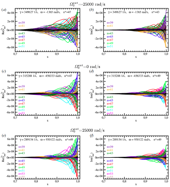

 Open access