


Highlights
What is already known?
-
• The bivariate linear mixed effects model (BLMM) using logit-transformed sensitivity and specificity is the standard approach in meta-analysis of diagnostic test accuracy (DTA) studies.
-
• However, BLMM has limitations, such as reliance on Haldane–Anscombe correction and approximate within-study variance estimates, especially problematic for meta-analyses with small or sparse studies.
-
• The bivariate generalized linear mixed model (BGLMM) offers a different framework but often faces convergence issues when meta-analyses are small or sparse.
What is new?
-
• The article proposes a novel exact method for within-study variance calculation that:
-
– does not require Haldane–Anscombe correction,
-
– is transformation-invariant, and
-
– works well regardless of sample size or number of studies.
-
-
• The method is evaluated against existing models using both real and simulated datasets.
Potential impact for RSM readers
-
• Readers involved in meta-analysis of DTA studies will gain a more accurate and flexible toolset, particularly for small or sparse datasets, where existing models often break down.
-
• The proposed exact method may reduce bias and improve the reliability of inference to support better clinical and methodological decisions based on DTA meta-analyses.
-
• The work helps to advance the methodological frontier in synthesis science, thereby addressing a persistent practical challenge in diagnostic research.
1 Introduction
Diagnostic tests or screening tests are essential in clinical practice for identifying individuals who have diseases and those who do not. The accuracy of these tests and the appropriateness of the thresholds employed to define positive results are assessed by diagnostic test accuracy (DTA) studies.Reference Croft, Altman and Deeks
1
These studies present a range of diagnostic accuracy metrics that are obtained by comparing the relevant diagnostic test (index test) result to the gold standard, which is the test that can accurately differentiate between people who are positive for a disease and those who are not. A diagnostic test is considered inaccurate if it yields a positive result for a patient who does not have the condition or a negative result for a patient who does have a condition. Therefore, it is essential to compare a diagnostic test’s accuracy to that of the reference or gold standard test to mitigate the risk of misdiagnosis. The results of DTA studies are composed of the probability of a positive test result in diseased individuals (sensitivity) and the probability of a negative test result in healthy individuals (specificity). The sensitivity (
 $Se$
) and specificity (
$Se$
) and specificity (
 $Sp$
) are the two main DTA metrics that indicate the diagnostic performance of the index test.Reference Binney, Hyde and Bossuyt
2
$Sp$
) are the two main DTA metrics that indicate the diagnostic performance of the index test.Reference Binney, Hyde and Bossuyt
2
Diagnostic tests in research often encounter errors and bias, which can complicate clinical decision-making. Meta-analyses address this by synthesizing data from multiple studies to provide reliable assessments of diagnostic performance, mitigating errors, and accounting for study heterogeneity. Meta-analysis is a statistical method for combining evidence from multiple studies that aim to address the same research question.Reference Borenstein, Cooper, Hedges and Valentine
3
Diagnostic test meta-analyses are crucial for evaluating the performance of specific diagnostic tests by combining data from multiple DTA studies.Reference Zar, Alsharif and Zar
4
This method considered the highest level of study design in medical research, enabling clinicians to make informed decisions based on robust evidence.Reference Haidich
5
In an aggregate data meta-analysis (ADMA) of DTA studies, information on the true positive (TP), true negative (TN), false positive (FP), and false negative (FN) outcomes for a particular diagnostic test across multiple studies is collected.Reference Zhao, Khan and Negeri
6
From this data, one can derive study-specific observed values for
 $Se$
,
$Se$
,
 $Sp$
, and other diagnostic accuracy measures. Researchers then combine data from multiple studies to generate comprehensive estimates of these test accuracy measures, taking into account the variability and potential biases of each study.
$Sp$
, and other diagnostic accuracy measures. Researchers then combine data from multiple studies to generate comprehensive estimates of these test accuracy measures, taking into account the variability and potential biases of each study.
Various statistical models for meta-analysis of DTA have been developed over the past two decades, each with its strengths and weaknesses. Bivariate random-effects and hierarchical models have also been developed during the last two decades to synthesize DTA measures, particularly logit-transformed
 $Se$
and
$Se$
and
 $Sp$
. Reitsma et al.’sReference Reitsma, Glas, Rutjes, Scholten, Bossuyt and Zwinderman
7
approach is easier to use and less complicated than Rutter and Gatsonis’sReference Rutter and Gatsonis
8
hierarchical model. Both models are parameterization of one another without covariates, and when applied to the same data, they produce similar results (Negeri et al.).Reference Negeri, Shaikh and Beyene
9
However, their development and parameter estimation methods are different: Rutter and Gatsonis’ model uses a Bayesian approach, whereas Reitsma et al.’s model uses a classical Frequentist approach. The standard bivariate linear mixed model (BLMM) of Reitsma et al.Reference Reitsma, Glas, Rutjes, Scholten, Bossuyt and Zwinderman
7
meta-analyzes DTA using maximum likelihood estimates (MLEs) through numerical optimization methods, as the model lacks a closed-form solution for the between-study heterogeneity parameter. A bivariate random effects model that utilizes the logit transformation of
$Sp$
. Reitsma et al.’sReference Reitsma, Glas, Rutjes, Scholten, Bossuyt and Zwinderman
7
approach is easier to use and less complicated than Rutter and Gatsonis’sReference Rutter and Gatsonis
8
hierarchical model. Both models are parameterization of one another without covariates, and when applied to the same data, they produce similar results (Negeri et al.).Reference Negeri, Shaikh and Beyene
9
However, their development and parameter estimation methods are different: Rutter and Gatsonis’ model uses a Bayesian approach, whereas Reitsma et al.’s model uses a classical Frequentist approach. The standard bivariate linear mixed model (BLMM) of Reitsma et al.Reference Reitsma, Glas, Rutjes, Scholten, Bossuyt and Zwinderman
7
meta-analyzes DTA using maximum likelihood estimates (MLEs) through numerical optimization methods, as the model lacks a closed-form solution for the between-study heterogeneity parameter. A bivariate random effects model that utilizes the logit transformation of
 $Se$
and
$Se$
and
 $Sp$
, and accounts for both within- and between-study heterogeneity is commonly used to make statistical inferences about the unknown test characteristics. However, it has been well reported that this model may lead to misleading inference,Reference Zhao, Khan and Negeri
6
,
Reference Trikalinos, Trow and Schmid
10
–
Reference Li, Lin, Cappelleri, Chu and Chen
12
particularly with small sample sizes or zero cell counts for TPs, TNs, FNs and FPs, requiring an arbitrary Haldane–Anscombe correctionReference Haldane
13
,
Reference Anscombe
14
when the data are sparse. Also, the logit transformed
$Sp$
, and accounts for both within- and between-study heterogeneity is commonly used to make statistical inferences about the unknown test characteristics. However, it has been well reported that this model may lead to misleading inference,Reference Zhao, Khan and Negeri
6
,
Reference Trikalinos, Trow and Schmid
10
–
Reference Li, Lin, Cappelleri, Chu and Chen
12
particularly with small sample sizes or zero cell counts for TPs, TNs, FNs and FPs, requiring an arbitrary Haldane–Anscombe correctionReference Haldane
13
,
Reference Anscombe
14
when the data are sparse. Also, the logit transformed
 $Se$
and
$Se$
and
 $Sp$
within each study are approximated to a normal distribution,Reference Chu and Cole
15
and these assumptions might not be valid in certain cases, such as small sample sizes or rare events. Alternative transformations which do not require Haldane–Anscombe correction, such as the arcsine square root (ASR) and Freeman–Tukey double arcsine (FTDA), were recently proposed by Negeri et al.Reference Negeri, Shaikh and Beyene
9
in the context of bivariate ADMA of DTA studies. However, these methods also suffer from using approximate or asymptotic within-study variance estimates, which can only be justified when within-study sample sizes are large.
$Sp$
within each study are approximated to a normal distribution,Reference Chu and Cole
15
and these assumptions might not be valid in certain cases, such as small sample sizes or rare events. Alternative transformations which do not require Haldane–Anscombe correction, such as the arcsine square root (ASR) and Freeman–Tukey double arcsine (FTDA), were recently proposed by Negeri et al.Reference Negeri, Shaikh and Beyene
9
in the context of bivariate ADMA of DTA studies. However, these methods also suffer from using approximate or asymptotic within-study variance estimates, which can only be justified when within-study sample sizes are large.
Chu and ColeReference Chu and Cole 15 developed a bivariate generalized linear mixed model (BGLMM) to avoid the within-studies normality assumption required by the BLMM of Reitsma et al.Reference Reitsma, Glas, Rutjes, Scholten, Bossuyt and Zwinderman 7 The BGLMM uses the exact binomial distribution and does not require Haldane–Anscombe correction when any of the four cell frequencies in a DTA study contain zero counts.Reference Zhao, Khan and Negeri 6 It provides unbiased and efficient estimates,Reference Harbord, Deeks, Egger, Whiting and Sterne 16 especially with sparse data or small sample sizes, without requiring logit transformation or normality assumptions to describe within-study variation in test characteristics.Reference Chu, Guo and Zhou 17 However, the BGLMM for sparse data meta-analyses may fail to converge or provide unreliable parameters, leading to overestimated results due to publication bias.Reference Zar, Alsharif and Zar 4 Additionally, if only a few studies exist, the BGLMM may underestimate variance and is not recommended due to variations in thresholds, spectrum effect, and systematic error.Reference Zar, Alsharif and Zar 4 Moreover, the BGLMM may cause convergence issues during parameter estimation, especially when dealing with a large number of parameters or a limited number of studies.Reference Rosenberger, Chu and Lin 18
To address the limitations of existing methods, we propose an exact or analytical within-study variance calculation approach that does not require a Haldane–Anscombe correction and remains invariant to transformations. To the best of our knowledge, there is no literature evaluating the performance of this analytical method in the context of an ADMA of DTA studies. The proposed analytical method avoids convergence issues and addresses the shortcomings of the standard BLMM, which often necessitates a Haldane–Anscombe correction when small or zero cell counts are present in the DTA data. To fill this research gap, this study aimed to evaluate the performance of the proposed exact within-study variance calculation method compared to the existing standard approaches for ADMA of DTA studies. A comprehensive simulation study evaluated the new exact method and the existing asymptotic approaches in terms of absolute bias, root mean squared error (RMSE), coverage probability, and 95% confidence interval (CI) width.
The remainder of this article is structured as follows: Section 2 presents motivating examples using two real-life datasets. Section 3 introduces the statistical methods and our simulation study design. In Section 4, we discuss the outcomes of our simulation study and illustrate the proposed within-study variance calculation method using two real-life datasets. Finally, we give a summary and concluding thoughts in Section 5.
2 Motivating examples
This section provides an overview of two real-life datasets from Doria et al.Reference Doria, Moineddin and Kellenberger
19
and Arevalo-Rodriguez et al.Reference Arevalo-Rodriguez, Smailagic and Roqué
20
to motivate the statistical methods presented in Section 3. Section 4 will analyze these datasets further to demonstrate the applicability of the techniques covered in this manuscript. These datasets were selected to compare the proposed within-study variance calculation method with standard approaches when data with zero cell counts are present and absent. We display a forest plot for each dataset showing the studies under consideration, their 95% CIs, and test characteristics (i.e., observed
 $Se$
or
$Se$
or
 $Sp$
).
$Sp$
).
2.1 The US-Children data
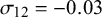
The first dataset is about the ultrasonography test. Doria et al.Reference Doria, Moineddin and Kellenberger
19
examined the effectiveness of this test in diagnosing appendicitis in both children and adults. The children-specific version of the ultrasonography data (US-Children) includes 23 studies, with an average of 77 children with appendicitis and 254 children without appendicitis across the studies (see Table A.1 in the Supplementary Material). In this dataset, there is an indication of sparsity in the counts of both FNs and FPs. Specifically, three of the primary studies (Cha et al.Reference Cha, Kim and Lee
21
; Lowe et al.Reference Lowe, Penney and Stein
22
; HanReference Han
23
) reported an observed
 $Se$
of 100% (i.e., had FNs=0) and one study (Siegel et al.Reference Siegel, Carel and Surratt
24
) reported an observed
$Se$
of 100% (i.e., had FNs=0) and one study (Siegel et al.Reference Siegel, Carel and Surratt
24
) reported an observed
 $Sp$
of 100% (i.e., had FP=0). The forest plot of the US-Children data is given in Figure 1.
$Sp$
of 100% (i.e., had FP=0). The forest plot of the US-Children data is given in Figure 1.

Figure 1 Forest plot for sensitivity (left) and specificity (right) of the US-Children data obtained after a Haldane–Anscombe correction is applied.
2.2 The mini-mental state examination data
The second meta-analysis is from the review by Arevalo-Rodriguez et al.,Reference Arevalo-Rodriguez, Smailagic and Roqué
20
which examined the mini-mental state examination (MMSE) test for detecting Alzheimer’s disease and dementia in people with mild cognitive impairment. The MMSE data includes eight studies, with an average of 47 participants with and 95 without the condition (see Table A.2 in the Supplementary Material). This meta-analysis showed no indication of sparsity in either counts of FNs or FPs; that is, none of the included primary studies had observed
 $Se$
or
$Se$
or
 $Sp$
values close to 0 or 1. Figure 2 displays the forest plot of the MMSE data.
$Sp$
values close to 0 or 1. Figure 2 displays the forest plot of the MMSE data.

Figure 2 Forest plot for sensitivity (left) and specificity (middle) of the Mini-Mental State Examination (MMSE) data obtained without applying a Haldane–Anscombe correction.
3 Methods
Given the observed data for any DTA study as in Table 1, we can easily estimate the diagnostic test’s accuracy parameters of interest as follows:
 $\widehat {Se}=TP/n_1$
and
$\widehat {Se}=TP/n_1$
and
 $\widehat {Sp}=TN/n_2$
, where
$\widehat {Sp}=TN/n_2$
, where
 $n_1$
and
$n_1$
and
 $n_2$
are the study-specific sample sizes that denote the total number of diseased and non-diseased individuals, respectively. In the following sections, we describe the standard methods for ADMA of DTA studies assuming the data structure presented in Table 1.
$n_2$
are the study-specific sample sizes that denote the total number of diseased and non-diseased individuals, respectively. In the following sections, we describe the standard methods for ADMA of DTA studies assuming the data structure presented in Table 1.
Table 1 Data structure of a diagnostic test result for a single study

3.1 The bivariate linear mixed-effects model
The BLMM of Reitsma et al.Reference Reitsma, Glas, Rutjes, Scholten, Bossuyt and Zwinderman 7 models both the within- and between-study variability in test characteristics using the bivariate normal distribution.
According to the BLMM, the observed vector of response for study i,
 $\mathbf {y}_i = (y_{1i}, y_{2i})^T=\left [\text {g}(\widehat {Se_i}), \text {g}(\widehat {Sp_i})\right ]^T$
, is modeled within-study in the following way:
$\mathbf {y}_i = (y_{1i}, y_{2i})^T=\left [\text {g}(\widehat {Se_i}), \text {g}(\widehat {Sp_i})\right ]^T$
, is modeled within-study in the following way:
 $$ \begin{align} \mathbf{y}_i|\boldsymbol{\mathcal{\mu}}_i \sim N_2\left[\boldsymbol{\mathcal{\mu}}_i= \begin{pmatrix} \mathcal{\phi}_{1i} \\ \mathcal{\phi}_{2i} \end{pmatrix}, \boldsymbol{S_i}= \begin{pmatrix} s_{1i}^2 & 0 \\ 0 & s_{2i}^2 \end{pmatrix} \right], \quad i=1,\ldots,k, \end{align} $$
where g is any transformation, such as the logit,
 $\boldsymbol {\phi }_{1i}$
denotes the true study-specific
$\boldsymbol {\phi }_{1i}$
denotes the true study-specific
 $\text {g}(Se_i)$
,
$\text {g}(Se_i)$
,
 $\boldsymbol {\phi }_{2i}$
denotes the true study-specific
$\boldsymbol {\phi }_{2i}$
denotes the true study-specific
 $\text {g}(Sp_i)$
,
$\text {g}(Sp_i)$
,
 $\mathbf {S}_i = \begin {pmatrix} s_{1i}^2 & 0 \\0 & s_{2i}^2 \end {pmatrix}$
represents the assumed to be known within-study variance–covariance matrix of the response vector
$\mathbf {S}_i = \begin {pmatrix} s_{1i}^2 & 0 \\0 & s_{2i}^2 \end {pmatrix}$
represents the assumed to be known within-study variance–covariance matrix of the response vector
 $\mathbf {y}_i,$
and k denotes the number of studies. In practice, however,
$\mathbf {y}_i,$
and k denotes the number of studies. In practice, however,
 $\boldsymbol {S_i}$
is estimated from the data using the first-order delta method (i.e., for logit, ASR, and FTDA).
$\boldsymbol {S_i}$
is estimated from the data using the first-order delta method (i.e., for logit, ASR, and FTDA).
At the second stage, the BLMM assumes heterogeneity between the true study-specific
 $\text {g}(Se_i)$
and
$\text {g}(Se_i)$
and
 $\text {g}(Sp_i)$
. Thus,
$\text {g}(Sp_i)$
. Thus,
 $$ \begin{align} \boldsymbol{\mu}_i= \begin{pmatrix} \phi_{1i} \\ \phi_{2i} \end{pmatrix} \sim \mathrm{N}_2\left[\boldsymbol{\mu}= \begin{pmatrix} \mu_1 \\ \mu_2 \end{pmatrix}, \boldsymbol{\Sigma}= \begin{pmatrix} \sigma_1^2 & \sigma_{12} \\ \sigma_{12} & \sigma_2^2 \end{pmatrix} \right], \quad i=1,2,\ldots,k, \end{align} $$
where
 $\boldsymbol {\mu }= \begin {pmatrix} \mu _1 \\ \mu _2 \end {pmatrix}$
denotes the true mean of
$\boldsymbol {\mu }= \begin {pmatrix} \mu _1 \\ \mu _2 \end {pmatrix}$
denotes the true mean of
 $\text {g}(Se_i)$
and
$\text {g}(Se_i)$
and
 $\text {g}(Sp_i)$
, and
$\text {g}(Sp_i)$
, and
 $\boldsymbol {\Sigma } = \begin {pmatrix} \sigma _1^2 & \sigma _{12} \\ \sigma _{12} & \sigma _2^2 \end {pmatrix}$
is the between-study covariance matrix, which denotes the heterogeneity parameter such that
$\boldsymbol {\Sigma } = \begin {pmatrix} \sigma _1^2 & \sigma _{12} \\ \sigma _{12} & \sigma _2^2 \end {pmatrix}$
is the between-study covariance matrix, which denotes the heterogeneity parameter such that
 $\sigma _1^2$
and
$\sigma _1^2$
and
 $\sigma _2^2$
are the variances of
$\sigma _2^2$
are the variances of
 $\phi _{1i}$
and
$\phi _{1i}$
and
 $\phi _{2i}$
, respectively, and
$\phi _{2i}$
, respectively, and
 $\sigma _{12}$
is the covariance between
$\sigma _{12}$
is the covariance between
 $\phi _{1i}$
and
$\phi _{1i}$
and
 $\phi _{2i}$
.
$\phi _{2i}$
.
By combining (3.1) and (3.2) and assuming that the studies are independent, we arrive at the marginal model
 $$ \begin{align} \mathbf{y}_i\sim N_2\left(\boldsymbol{\mu}, \boldsymbol{\Sigma}_i\right), i=1,\ldots,k, \end{align} $$
where
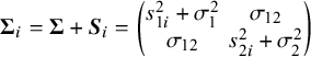 $ \boldsymbol {\Sigma }_i =\boldsymbol {\Sigma }+\boldsymbol {S}_i= \begin {pmatrix} s_{1i}^2+\sigma _1^2 & \sigma _{12} \\ \sigma _{12} & s_{2i}^2+\sigma _2^2 \end {pmatrix} $
.
$ \boldsymbol {\Sigma }_i =\boldsymbol {\Sigma }+\boldsymbol {S}_i= \begin {pmatrix} s_{1i}^2+\sigma _1^2 & \sigma _{12} \\ \sigma _{12} & s_{2i}^2+\sigma _2^2 \end {pmatrix} $
.
3.1.1 The approximate or asymptotic variance estimation methods
The standard BLMM Reference Reitsma, Glas, Rutjes, Scholten, Bossuyt and Zwinderman
7
employs the logit transformation to model the observed
 $Se$
and
$Se$
and
 $Sp$
using the bivariate normal distribution. Thus, for the within-study variance of a logit-transformed proportion estimate,
$Sp$
using the bivariate normal distribution. Thus, for the within-study variance of a logit-transformed proportion estimate,
 $\text {g}(\hat {p}_{ji})=\text {logit}(\hat {p}_{ji}), i=1,\ldots ,k$
, usually the delta method based on the first-order Taylor series approximation is usedReference Negeri, Shaikh and Beyene
9
,
Reference Rücker, Schwarzer, Carpenter and Olkin
25
:
$\text {g}(\hat {p}_{ji})=\text {logit}(\hat {p}_{ji}), i=1,\ldots ,k$
, usually the delta method based on the first-order Taylor series approximation is usedReference Negeri, Shaikh and Beyene
9
,
Reference Rücker, Schwarzer, Carpenter and Olkin
25
:
 $$ \begin{align*} s_{ji}^2 &= \text{Var}[\text{logit}(\hat{p}_{ji})] \\ &\approx \text{Var}(\hat{p}_{ji}) \left\{\frac{\partial}{\partial \hat{p}_{ji}} [\text{logit}(\hat{p}_{ji})]\right\}^2 \\ &=\text{Var}(\hat{p}_{ji}) \left\{\frac{\partial}{\partial \hat{p}_{ji}} \left[\text{log}\left(\frac{\hat{p}_{ji}}{1-\hat{p}_{ji}}\right)\right]\right\}^2 \\ &= \frac{\hat{p}_{ji} (1-\hat{p}_{ji})}{n_{ji}} \left[\frac{1}{\hat{p}_{ji} (1-\hat{p}_{ji})}\right]^2 \\ &= \frac{1}{n_{ji} \hat{p}_{ji} (1-\hat{p}_{ji})}, \text{ for } j=1,2 \text{ and } i=1,\ldots,k. \end{align*} $$
The above expression implies that the variance estimate of logit
 $(\hat {p}_{ji})$
is defined only if the
$(\hat {p}_{ji})$
is defined only if the
 $\hat {p}_{ji}$
is different from
$\hat {p}_{ji}$
is different from
 $0$
and
$0$
and
 $1$
; that is, only if there are no zero cell counts in Table 1. Otherwise, usually, 0.5 is added to all cells of the
$1$
; that is, only if there are no zero cell counts in Table 1. Otherwise, usually, 0.5 is added to all cells of the
 $2\times 2$
contingency table. Negeri et al.Reference Negeri, Shaikh and Beyene
9
proposed two additional transformations, the ASR and FTDA transformations,Reference Freeman and Tukey
26
to overcome the limitations of the default logit transformation used by the BLMM. The respective approximate within-study variances for the ASR and FTDA transformations were given by
$2\times 2$
contingency table. Negeri et al.Reference Negeri, Shaikh and Beyene
9
proposed two additional transformations, the ASR and FTDA transformations,Reference Freeman and Tukey
26
to overcome the limitations of the default logit transformation used by the BLMM. The respective approximate within-study variances for the ASR and FTDA transformations were given by
 $\frac {1}{4n_{ji}}$
and
$\frac {1}{4n_{ji}}$
and
 $\frac {1}{4n_{ji}+2}$
, for
$\frac {1}{4n_{ji}+2}$
, for
 $j=1,2$
and
$j=1,2$
and
 $i = 1,\ldots ,k$
.
$i = 1,\ldots ,k$
.
3.1.2 The proposed exact or analytical variance calculation method
All three of the above within-study variance estimation methods are based on asymptotic results that can only be valid for a large number of studies in a meta-analysis. Moreover, the standard BLMM with the logit transformation requires a Haldane–Anscombe correction for sparse studies in a meta-analysis. Therefore, we propose a within-study variance calculation approach based on exact or analytical resultsReference Kasuya
27
for ADMA, which works for any transformation and meta-analysis size. The exact variance
 $\text{Var}[\text {g}(X)]$
for a given DTA frequency count
$\text{Var}[\text {g}(X)]$
for a given DTA frequency count
 $TP=X$
or
$TP=X$
or
 $TN=X$
of a function
$TN=X$
of a function
 $\text {g}$
can be calculated using the theoretical variance formula as
$\text {g}$
can be calculated using the theoretical variance formula as
 $$ \begin{align} \text{ Var}[\text{g}(X)]=E[\text{g}(X)^2]-[E(\text{g}(X))]^2, \end{align} $$
where the function
 $\text {g}$
can be any transformation, including the logit, ASR, or FTDA. Assuming the Binomial distribution for the counts in Table 1, given the study-specific sensitivity
$\text {g}$
can be any transformation, including the logit, ASR, or FTDA. Assuming the Binomial distribution for the counts in Table 1, given the study-specific sensitivity
 $(p_{1i}=\frac {X}{n_{1i}})$
or specificity
$(p_{1i}=\frac {X}{n_{1i}})$
or specificity
 $(p_{2i}=\frac {X}{n_{2i}})$
and the total number of participants with disease
$(p_{2i}=\frac {X}{n_{2i}})$
and the total number of participants with disease
 $(n_{1i})$
and without disease
$(n_{1i})$
and without disease
 $(n_{2i})$
, we define our within-study variance formula using the following finite Binomial sums:
$(n_{2i})$
, we define our within-study variance formula using the following finite Binomial sums:
 $$ \begin{align} s_{ji}^2 = \operatorname{Var}\!\left[g\!\left(p_{ji}=\tfrac{X}{n_{ji}}\right)\right] &= \sum_{x=0}^{n_{ji}} \Bigg[g\!\left(\tfrac{x}{n_{ji}}\right)\Bigg]^2 \binom{n_{ji}}{x} p_{ji}^x (1-p_{ji})^{\,n_{ji}-x} \notag \\ &\quad - \left\{\sum_{x=0}^{n_{ji}} g\!\left(\tfrac{x}{n_{ji}}\right) \binom{n_{ji}}{x} p_{ji}^x (1-p_{ji})^{\,n_{ji}-x}\right\}^2, \end{align} $$
for
 $j=1,2$
and
$j=1,2$
and
 $i=1,\ldots ,k$
, where the function
$i=1,\ldots ,k$
, where the function
 $g(p_{ji})$
is defined as
$g(p_{ji})$
is defined as
 $$\begin{align*}g(p_{ji}) = \begin{cases} \log\!\left(\dfrac{p_{ji}}{1-p_{ji}}\right), & \text{logit transformation}, \\[2ex] \sin^{-1}\!\big(\sqrt{p_{ji}}\big), & \text{ASR transformation}, \\[2ex] \dfrac{1}{2}\left\{\sin^{-1}\!\left(\sqrt{\dfrac{n_{ji}p_{ji}}{\,n_{ji}+1}}\right) + \sin^{-1}\!\left(\sqrt{\dfrac{n_{ji}p_{ji}+1}{\,n_{ji}+1}}\right)\right\}, & \text{FTDA transformation}. \end{cases} \end{align*}$$
In addition to the benefits listed above, unlike the BLMM of Reitsma et al.,Reference Reitsma, Glas, Rutjes, Scholten, Bossuyt and Zwinderman
7
the proposed analytical variance formula does not fail to converge or require Haldane–Anscombe correction for sparse studies in a meta-analysis. However, the proposed approach with logit transformation requires a Haldane–Anscombe correction for the smallest and largest value in the binomial range, that is, only when
 $x=0$
or
$x=0$
or
 $x=n_{ji}$
.
$x=n_{ji}$
.
3.2 The bivariate generalized linear mixed model
For completeness, we also describe the BGLMM of Chu and ColeReference Chu and Cole
15
as a comparator model to the BLMM and the proposed within-study variance calculation approach. In a BGLMM for ADMA, the variability within the study for
 $i=1,2,\ldots , k$
is modeled as
$i=1,2,\ldots , k$
is modeled as
 $$ \begin{align} &TP_{i}\mid Se_i\sim Binomial \left(n_{1i}, Se_{i}\right)\nonumber\\&TN_{i}\mid Sp_i\sim Binomial \left(n_{2i}, Sp_{i}\right), \end{align} $$
where the linear component and random effects have the form:
 $$\begin{align*}\text{g}\left(Se_{i}\right)=\mu_1+\phi_{1i} \text{ and }\text{g}\left(Sp_{i}\right)=\mu_{2}+\phi_{2i} \end{align*}$$
and
 $$ \begin{align}\boldsymbol{\mu}_i= \begin{pmatrix} \phi_{1i} \\ \phi_{2i} \end{pmatrix} \sim \mathrm{N}_2\left[\boldsymbol{\mu}= \begin{pmatrix} 0 \\ 0 \end{pmatrix}, \boldsymbol{\Sigma}= \begin{pmatrix} \sigma_1^2 & \sigma_{12} \\ \sigma_{12} & \sigma_2^2 \end{pmatrix} \right]. \end{align} $$
The BGLMM is recommended over the BLMM, as it performs better, especially for small meta-analyses and for values of
 $Se$
or
$Se$
or
 $Sp$
closer to 1 or 0.Reference Hamza, van Houwelingen and Stijnen
11
Hence, it is widely accepted as the preferred model for ADMA of DTAs, although it also suffers from convergence issues unless appropriate numerical optimization methods are used.Reference Zhao, Khan and Negeri
6
$Sp$
closer to 1 or 0.Reference Hamza, van Houwelingen and Stijnen
11
Hence, it is widely accepted as the preferred model for ADMA of DTAs, although it also suffers from convergence issues unless appropriate numerical optimization methods are used.Reference Zhao, Khan and Negeri
6
3.3 Parameter estimation
For the BLMM examined in this study, five parameters must be estimated to make statistical inferences: two fixed effects (
 $\mu _1$
and
$\mu _1$
and
 $\mu _2$
) and three random effects (
$\mu _2$
) and three random effects (
 $\sigma _1^2$
,
$\sigma _1^2$
,
 $\sigma _2^2$
, and
$\sigma _2^2$
, and
 $\sigma _{12}$
). For k independent studies, observed sensitivities
$\sigma _{12}$
). For k independent studies, observed sensitivities
 $(\widehat {Se}_i)$
and specificities
$(\widehat {Se}_i)$
and specificities
 $(\widehat {Sp}_i)$
; the adjusted likelihood function from which the maximum likelihood estimators are derived is given as follows.
$(\widehat {Sp}_i)$
; the adjusted likelihood function from which the maximum likelihood estimators are derived is given as follows.
The likelihood function L( μ , Σ ) is given by
 $$ \begin{align*} L(\boldsymbol{\mu, \Sigma}) &= \prod_{i=1}^{k} \frac{1}{\sqrt{2\pi}|\boldsymbol{\Sigma}_i|^{1/2}} \exp\left[-\frac{1}{2} (\mathbf{y}_i - \boldsymbol{\mu})^T \boldsymbol{\Sigma}_i^{-1} (\mathbf{y}_i - \boldsymbol{\mu})\right] \\ & = (2\pi)^{-k/2} \prod_{i=1}^{k} |\boldsymbol{\Sigma}_i|^{-1/2} \exp\left[-\frac{1}{2} (\mathbf{y}_i - \boldsymbol{\mu})^T \boldsymbol{\Sigma}_i^{-1} (\mathbf{y}_i - \boldsymbol{\mu})\right]. \end{align*} $$
The log-likelihood function is
 $$ \begin{align} \ell(\boldsymbol{\mu, \Sigma}) = -\frac{k}{2} \log(2\pi) - \frac{1}{2} \sum_{i=1}^{k} \log|\boldsymbol{\Sigma}_i| - \frac{1}{2} \sum_{i=1}^{k} (\mathbf{y}_i - \boldsymbol{\mu})^T \boldsymbol{\Sigma}_i^{-1} (\mathbf{y}_i - \boldsymbol{\mu}). \end{align} $$
To estimate the parameters of the bivariate random effects models, we employed maximum likelihood estimation via numerical optimization. Initial parameter values were set using empirical means and variance–covariance estimates from transformed data, providing data-driven starting parameter values for each model. Once the estimate of the between-study covariance matrix,
 $\boldsymbol{\hat{\Sigma}}$
, is obtained through numerical methods, the parameter of interest,
μ
, is estimated using the weighted average method, which is equivalent to the MLE:
$\boldsymbol{\hat{\Sigma}}$
, is obtained through numerical methods, the parameter of interest,
μ
, is estimated using the weighted average method, which is equivalent to the MLE:
 $$\begin{align*}\boldsymbol{\hat{\mu}}=\left(\sum_{i=1}^{k}(\boldsymbol{\hat{\Sigma}}+\boldsymbol{S}_i)^{-1}\right)^{-1}\sum_{i=1}^{k}(\boldsymbol{\hat{\Sigma}}+\boldsymbol{S}_i)^{-1}\mathbf{y}_i.\end{align*}$$
Asymptotically, the estimated average effect size,
 $\widehat {\boldsymbol {\mu }}$
, is approximately distributed as bivariate normal with mean
$\widehat {\boldsymbol {\mu }}$
, is approximately distributed as bivariate normal with mean
 $\boldsymbol {\mu }$
and variance–covariance,
$\boldsymbol {\mu }$
and variance–covariance,
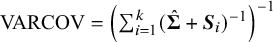 $\text {VARCOV}=\left (\sum _{i=1}^{k}(\hat {\boldsymbol {\Sigma }}+\boldsymbol {S}_i)^{-1}\right )^{-1}$
. Therefore, the approximate 100(1 − α)% CI for μ
j
can be obtained as
$\text {VARCOV}=\left (\sum _{i=1}^{k}(\hat {\boldsymbol {\Sigma }}+\boldsymbol {S}_i)^{-1}\right )^{-1}$
. Therefore, the approximate 100(1 − α)% CI for μ
j
can be obtained as
 $$\begin{align*}\left(\hat{{\mu}}_j - Z_{\frac{\alpha}{2}} \sqrt{\text{VARCOV}(j, j)}, \quad \hat{{\mu}}_j + Z_{\frac{\alpha}{2}} \sqrt{\text{VARCOV}(j, j)}\right), \end{align*}$$
where
 $Z_{\frac {\alpha }{2}}$
is the upper
$Z_{\frac {\alpha }{2}}$
is the upper
 $\frac {\alpha }{2}$
th percentile of the standard normal distribution and VARCOV
$\frac {\alpha }{2}$
th percentile of the standard normal distribution and VARCOV
 $(j, j)$
is the jth diagonal element of VARCOV.
$(j, j)$
is the jth diagonal element of VARCOV.
For the BGLMM, its marginal likelihood function can be written as
 $$ \begin{align} L\left(TP_i,TN_i \mid \boldsymbol{\mu,\Sigma}\right) &= \prod_{i=1}^{k} \int_{0}^{1} \int_{0}^{1} \text{Binomial}\left(n_{1i}, Se_i\right) \text{Binomial}\left(n_{2i}, Sp_i\right) \notag \\ &\quad \times \phi_2\left(g(Se_i), g(Sp_i); \boldsymbol{\mu, \Sigma} \right) \, \partial Se_i \, \partial Sp_i. \end{align} $$
However, the marginal likelihood function in (3.9) does not have a closed-form solution. Therefore, numerical algorithms like the Laplace approximation (LA),Reference Pinheiro and Bates 28 , Reference Liu and Pierce 29 iteratively reweighted least square (ILRS),Reference Jorgensen 30 and adaptive Gauss–Hermite quadrature (AGHQ),Reference Pinheiro and Bates 28 which numerically integrate the likelihood, were used.Reference Zhao, Khan and Negeri 6 Since a recent study by Zhao et al.Reference Zhao, Khan and Negeri 6 recommended against using the LA in situations where data sparsity is a concern and suggested using either the IRLS or AGHQ regardless of data characteristics, we decided to use the IRLS as the primary computational method for this manuscript since it had a higher convergence rate than the AGHQ.
Furthermore, we constructed the summary receiver operating characteristics (SROC) curve and its area under the SROC curve (AUC) for the two motivating examples, following the approach of Chu et al.Reference Chu, Guo and Zhou
17
Under the assumption of bivariate normality of
 $[g(Se_i), g(Sp_i)]$
, the expected sensitivity for a chosen specificity on the transformed scale is given by
$[g(Se_i), g(Sp_i)]$
, the expected sensitivity for a chosen specificity on the transformed scale is given by
 $$ \begin{align} g(Se_i) = \mu_1 - \frac{\sigma_{12}}{\sigma_2^2}\mu_2 + \frac{\sigma_{12}}{\sigma_2^2} g(Sp_i). \end{align} $$
Accordingly, the expected AUC is approximated by
 $$ \begin{align} AUC = \int_0^1 g^{-1}\left\{\mu_1 - \frac{\sigma_{12}}{\sigma_2^2}\mu_2 + \frac{\sigma_{12}}{\sigma_2^2} g(Sp_i)\right\} \, dSp_i. \end{align} $$
3.4 Simulation study design
In this study, we developed a four-step simulation based on a strategy proposed by Zhao et al.Reference Zhao, Khan and Negeri
6
We considered three (small, medium, and large) pairs of true mean sensitivity and specificity
 $\left (Se, Sp\right )$
, the true between-study variances
$\left (Se, Sp\right )$
, the true between-study variances
 $\left (\sigma _1^2, \sigma _2^2\right )$
and covariance
$\left (\sigma _1^2, \sigma _2^2\right )$
and covariance
 $(\sigma _{12})$
, the true sample sizes
$(\sigma _{12})$
, the true sample sizes
 $\left (n_1, n_2\right )$
for each study, and four different numbers of studies in the meta-analysis (k) as the true parameters. The specific settings are as given in Table 2. Accordingly, we explored a total of
$\left (n_1, n_2\right )$
for each study, and four different numbers of studies in the meta-analysis (k) as the true parameters. The specific settings are as given in Table 2. Accordingly, we explored a total of
 $3^4\times 4=324$
scenarios in our simulation investigation and for each combination of parameters, DTA datasets were generated using three true models: bivariate normal distribution using the logit, ASR, and FTDA transformation, following the methodology outlined by Negeri et al.Reference Negeri, Shaikh and Beyene
9
The simulation was run 1000 times using different seeds for each replication to ensure reproducibility. We evaluated the models in terms of accuracy (bias), precision (RMSE), coverage (95% empirical coverage probability), and 95% CI width.
$3^4\times 4=324$
scenarios in our simulation investigation and for each combination of parameters, DTA datasets were generated using three true models: bivariate normal distribution using the logit, ASR, and FTDA transformation, following the methodology outlined by Negeri et al.Reference Negeri, Shaikh and Beyene
9
The simulation was run 1000 times using different seeds for each replication to ensure reproducibility. We evaluated the models in terms of accuracy (bias), precision (RMSE), coverage (95% empirical coverage probability), and 95% CI width.
Table 2 True parameter settings for the simulation study

3.5 Software
Three R packages were utilized for data simulation and statistical analyses. The faraway packageReference Faraway
31
was used to both transform and back-transform the simulated
 $Se$
and
$Se$
and
 $Sp$
within the models. The mada packageReference Doebler
32
was used to create forest plots for the real-life data examples. Bivariate data from the bivariate normal distribution were simulated using the mvrnorm function from the MASS package.Reference Ripley
33
,
Reference Ripley, Venables and Bates
34
We applied the IRLS with nAGQ equal to 0 using the glmer() function from the lme4 R packageReference Bates, Mächler, Bolker and Walker
35
to fit the BGLMM. We wrote an R code to fit the BLMM and proposed models.
$Sp$
within the models. The mada packageReference Doebler
32
was used to create forest plots for the real-life data examples. Bivariate data from the bivariate normal distribution were simulated using the mvrnorm function from the MASS package.Reference Ripley
33
,
Reference Ripley, Venables and Bates
34
We applied the IRLS with nAGQ equal to 0 using the glmer() function from the lme4 R packageReference Bates, Mächler, Bolker and Walker
35
to fit the BGLMM. We wrote an R code to fit the BLMM and proposed models.
4 Results
4.1 Simulation study results
This Section presents simulation results for scenarios characterized by small sample sizes per group, large between-study variability in logit-sensitivity and logit-specificity, and a small negative correlation between them, reflecting characteristics of our real-life data examples. Simulation results for the remaining scenarios are provided in the Supplementary Material.
Figure 3 displays the bias of the overall
 $Se$
and
$Se$
and
 $Sp$
estimators for the proposed exact within-study variance calculation method and the existing approaches, given the true parameters
$Sp$
estimators for the proposed exact within-study variance calculation method and the existing approaches, given the true parameters
 $\mathcal {\sigma }_1^2=1.59$
,
$\mathcal {\sigma }_1^2=1.59$
,
 $\mathcal {\sigma }_2^2=1.83$
, and
$\mathcal {\sigma }_2^2=1.83$
, and
 $\mathcal {\sigma }_{12}=-0.7$
. The BLMM based on the proposed exact within-study variance calculation method and arcsine transformations (Exact-ASR and Exact-FTDA) yielded unbiased estimates of overall
$\mathcal {\sigma }_{12}=-0.7$
. The BLMM based on the proposed exact within-study variance calculation method and arcsine transformations (Exact-ASR and Exact-FTDA) yielded unbiased estimates of overall
 $Se$
and
$Se$
and
 $Sp$
when the meta-analysis did not contain sparse primary studies (Figure 3, first two panels). When the meta-analysis had sparse primary studies (Figure 3, third panel), while the Exact-Logit had the smallest bias for
$Sp$
when the meta-analysis did not contain sparse primary studies (Figure 3, first two panels). When the meta-analysis had sparse primary studies (Figure 3, third panel), while the Exact-Logit had the smallest bias for
 $Se$
, the Exact-Logit and the BGLMM had the smallest bias for
$Se$
, the Exact-Logit and the BGLMM had the smallest bias for
 $Sp$
. Conversely, the standard approximate BLMM-Logit had the largest negative bias for sensitivity and specificity, irrespective of the presence of sparse primary studies in a meta-analysis. Although similar results were observed when the number of participants was moderate (
$Sp$
. Conversely, the standard approximate BLMM-Logit had the largest negative bias for sensitivity and specificity, irrespective of the presence of sparse primary studies in a meta-analysis. Although similar results were observed when the number of participants was moderate (
 $n_1=100, n_2=200$
; Figure B.20 in the Supplementary Material) or large (
$n_1=100, n_2=200$
; Figure B.20 in the Supplementary Material) or large (
 $n_1=200, n_2=300$
; Figure B.21 in the Supplementary Material), the BLMM-Logit model’s bias diminished with increasing sample sizes, as expected.
$n_1=200, n_2=300$
; Figure B.21 in the Supplementary Material), the BLMM-Logit model’s bias diminished with increasing sample sizes, as expected.

Figure 3 Bias for sensitivity (Se) and specificity (Sp) when
 $\mathcal {\sigma }_1^2=1.59$
,
$\mathcal {\sigma }_1^2=1.59$
,
 $\mathcal {\sigma }_{12}=-0.03$
,
$\mathcal {\sigma }_{12}=-0.03$
,
 $\sigma _2^2=1.83$
,
$\sigma _2^2=1.83$
,
 $n_1=50,$
and
$n_1=50,$
and
 $n_2=100$
.
$n_2=100$
.
Figure 4 depicts the RMSE for each method’s overall
 $Se$
and
$Se$
and
 $Sp$
estimator. Relatively all methods had comparable RMSEs when there were no sparse primary studies in a meta-analysis (Figure 4, first two panels). However, the proposed Exact-Logit method and the standard BGLMM had the smallest RMSE for
$Sp$
estimator. Relatively all methods had comparable RMSEs when there were no sparse primary studies in a meta-analysis (Figure 4, first two panels). However, the proposed Exact-Logit method and the standard BGLMM had the smallest RMSE for
 $Se$
and
$Se$
and
 $SP$
when there were sparse primary studies in a meta-analysis (Figure 4, third panel). Conversely, the standard approximate BLMM-Logit model had the largest RMSE for
$SP$
when there were sparse primary studies in a meta-analysis (Figure 4, third panel). Conversely, the standard approximate BLMM-Logit model had the largest RMSE for
 $Se$
and
$Se$
and
 $SP$
for the latter scenario. Consistent results were observed for moderate (Figure C.20 in the Supplementary Material) and large (Figure C.21 in the Supplementary Material) numbers of participants in a meta-analysis study, although, as expected, the RMSEs improved with an increasing number of studies in the meta-analysis.
$SP$
for the latter scenario. Consistent results were observed for moderate (Figure C.20 in the Supplementary Material) and large (Figure C.21 in the Supplementary Material) numbers of participants in a meta-analysis study, although, as expected, the RMSEs improved with an increasing number of studies in the meta-analysis.

Figure 4 RMSE for sensitivity (Se) and specificity (Sp) when
 $\mathcal {\sigma }_1^2=1.59$
,
$\mathcal {\sigma }_1^2=1.59$
,
 $\mathcal {\sigma }_{12}=-0.03$
,
$\mathcal {\sigma }_{12}=-0.03$
,
 $\sigma _2^2=1.83$
,
$\sigma _2^2=1.83$
,
 $n_1=50,$
and
$n_1=50,$
and
 $n_2=100$
.
$n_2=100$
.
All methods had comparable 95% empirical coverage probability (Figure 5) when there were no sparse primary studies in the meta-analysis (first two panels), regardless of the other parameters varied in our simulation. However, when there were sparse primary studies in a meta-analysis (third panel), the proposed exact methods (Exact-Logit, Exact-ASR, and Exact-FTDA) and the BGLMM had superior coverage probabilities, achieving the nominal 95%, especially in
 $Se$
, compared to the traditional approximate BLMM-Logit method, which had a poor coverage probability for this scenario. Similar trends were observed when the number of participants in a meta-analytic study was moderate (Figure D.20 in the Supplementary Material) or large (Figure D.21 in the Supplementary Material), except that the coverage probabilities of the asymptotic BLMM-Logit improved with increasing sample sizes, as expected.
$Se$
, compared to the traditional approximate BLMM-Logit method, which had a poor coverage probability for this scenario. Similar trends were observed when the number of participants in a meta-analytic study was moderate (Figure D.20 in the Supplementary Material) or large (Figure D.21 in the Supplementary Material), except that the coverage probabilities of the asymptotic BLMM-Logit improved with increasing sample sizes, as expected.

Figure 5 Coverage probability for sensitivity (Se) and specificity (Sp) when
 $\mathcal {\sigma }_1^2=1.59$
,
$\mathcal {\sigma }_1^2=1.59$
,
 $\mathcal {\sigma }_{12}=-0.03$
,
$\mathcal {\sigma }_{12}=-0.03$
,
 $\mathcal {\sigma }_2^2=1.83$
,
$\mathcal {\sigma }_2^2=1.83$
,
 $n_1=50,$
and
$n_1=50,$
and
 $n_2=100$
.
$n_2=100$
.
In terms of 95% CI widths (Figure 6), we found that all methods had comparable average widths of the 95% CIs when the number of studies in a meta-analysis was large and the meta-analysis contained no sparse primary studies (Figure 6, first two panels). However, the standard asymptotic BLMM-Logit, the proposed Exact-Logit, and the BGLMM had narrower 95% CI widths when there were sparse primary studies in a meta-analysis (third panels). The Exact-ASR and Exact-FTDA had the narrowest 95% CI widths when there were no sparse primary studies and the number of studies was small (first two panels), regardless of the varied parameters in our simulations. Moreover, we observed that models based on the arcsine transformations (Exact-ASR and Exact-FTDA) had the widest 95% CI widths for meta-analyses with sparse primary studies, irrespective of the number of participants or studies in a meta-analysis. This trend was also observed for moderate (Figure E.20 in the Supplementary Material) and large (Figure E.21 in the Supplementary Material) sample sizes in a meta-analysis study.

Figure 6 CI widths for sensitivity (
 $Se$
) and specificity (
$Se$
) and specificity (
 $Sp$
) when
$Sp$
) when
 $\mathcal {\sigma }_1^2=1.59$
,
$\mathcal {\sigma }_1^2=1.59$
,
 $\mathcal {\sigma }_{12}=-0.03$
,
$\mathcal {\sigma }_{12}=-0.03$
,
 $\mathcal {\sigma }_2^2=1.83$
,
$\mathcal {\sigma }_2^2=1.83$
,
 $n_1=50,$
and
$n_1=50,$
and
 $n_2=100$
.
$n_2=100$
.
In terms of the bias of the between-study variances
 $\mathcal {\sigma }_1^2$
and
$\mathcal {\sigma }_1^2$
and
 $\mathcal {\sigma }_2^2$
, the proposed exact variance calculation methods (Exact-Logit, Exact-ASR, and Exact-FTDA) and the BGLMM outperformed the standard BLMM-Logit across all scenarios (Figure 7). The standard BLMM-Logit method significantly underestimated
$\mathcal {\sigma }_2^2$
, the proposed exact variance calculation methods (Exact-Logit, Exact-ASR, and Exact-FTDA) and the BGLMM outperformed the standard BLMM-Logit across all scenarios (Figure 7). The standard BLMM-Logit method significantly underestimated
 $\mathcal {\sigma }_1^2$
and
$\mathcal {\sigma }_1^2$
and
 $\mathcal {\sigma }_2^2$
across all scenarios, whereas the other methods provided more accurate estimates. Although the Exact-Logit method also underestimated
$\mathcal {\sigma }_2^2$
across all scenarios, whereas the other methods provided more accurate estimates. Although the Exact-Logit method also underestimated
 $\mathcal {\sigma }_2^2$
when there were sparse primary studies in a meta-analysis, its bias decreased for moderate or large number of participants per study, as expected (Figures F.20 and F.21 in the Supplementary Material).
$\mathcal {\sigma }_2^2$
when there were sparse primary studies in a meta-analysis, its bias decreased for moderate or large number of participants per study, as expected (Figures F.20 and F.21 in the Supplementary Material).

Figure 7 Bias for
 $\mathcal {\sigma }_1^2$
and
$\mathcal {\sigma }_1^2$
and
 $\mathcal {\sigma }_2^2 $
when the true
$\mathcal {\sigma }_2^2 $
when the true
 $\mathcal {\sigma }_1^2=1.59$
,
$\mathcal {\sigma }_1^2=1.59$
,
 $\mathcal {\sigma }_{12}=-0.03$
,
$\mathcal {\sigma }_{12}=-0.03$
,
 $\mathcal {\sigma }_2^2=1.83$
,
$\mathcal {\sigma }_2^2=1.83$
,
 $n_1=50,$
and
$n_1=50,$
and
 $n_2=100$
.
$n_2=100$
.
Considering the RMSE of
 $\mathcal {\sigma }_1^2$
and
$\mathcal {\sigma }_1^2$
and
 $\mathcal {\sigma }_2^2$
(Figure 8), the proposed exact method using the arcsine transformations (Exact-ASR and Exact-FTDA) had the least RMSE for
$\mathcal {\sigma }_2^2$
(Figure 8), the proposed exact method using the arcsine transformations (Exact-ASR and Exact-FTDA) had the least RMSE for
 $\mathcal {\sigma }_1^2$
and
$\mathcal {\sigma }_1^2$
and
 $\mathcal {\sigma }_2^2$
, irrespective of the presence or absence of sparse primary studies in a meta-analysis. However, while the standard asymptotic BLMM-Logit method had the worst RMSE when a meta-analysis contained sparse primary studies, the proposed Exact-Logit method and the BGLMM had the second least RMSEs. Similar trends were observed when the number of participants was moderate or large (Figures G.20 and G.21 in the Supplementary Material), which also revealed diminishing RMSEs as the sample sizes increased.
$\mathcal {\sigma }_2^2$
, irrespective of the presence or absence of sparse primary studies in a meta-analysis. However, while the standard asymptotic BLMM-Logit method had the worst RMSE when a meta-analysis contained sparse primary studies, the proposed Exact-Logit method and the BGLMM had the second least RMSEs. Similar trends were observed when the number of participants was moderate or large (Figures G.20 and G.21 in the Supplementary Material), which also revealed diminishing RMSEs as the sample sizes increased.

Figure 8 RMSE for
 $\mathcal {\sigma }_1^2$
and
$\mathcal {\sigma }_1^2$
and
 $\mathcal {\sigma }_2^2 $
when the true
$\mathcal {\sigma }_2^2 $
when the true
 $\sigma _1^2=1.59$
,
$\sigma _1^2=1.59$
,
 $\mathcal {\sigma }_{12}=-0.03$
,
$\mathcal {\sigma }_{12}=-0.03$
,
 $\sigma _2^2=1.83$
,
$\sigma _2^2=1.83$
,
 $n_1=50,$
and
$n_1=50,$
and
 $n_2=100$
.
$n_2=100$
.
Regarding bias and RMSE of the between-study covariance
 $(\mathcal {\sigma }_{12} )$
, all methods had comparable bias when there were no sparse primary studies (Figure 9, top row, first two panels). For meta-analysis with sparse primary studies, the proposed Exact-ASR and Exact-FTDA had the least bias, and the traditional approximate BLMM-Logit and the Exact-Logit had the largest bias. On the other hand, whereas the Exact-ASR and Exact-FTDA had the smallest RMSE, the Exact-Logit, BLMM-Logit, and BGLMM had the largest RMSE for
$(\mathcal {\sigma }_{12} )$
, all methods had comparable bias when there were no sparse primary studies (Figure 9, top row, first two panels). For meta-analysis with sparse primary studies, the proposed Exact-ASR and Exact-FTDA had the least bias, and the traditional approximate BLMM-Logit and the Exact-Logit had the largest bias. On the other hand, whereas the Exact-ASR and Exact-FTDA had the smallest RMSE, the Exact-Logit, BLMM-Logit, and BGLMM had the largest RMSE for
 $\mathcal {\sigma }_{12}$
. Similar patterns were observed when a meta-analysis study contained a moderate to large number of participants (Figures H.20 and H.21 in the Supplementary Material), which also resulted in improved bias and RMSE.
$\mathcal {\sigma }_{12}$
. Similar patterns were observed when a meta-analysis study contained a moderate to large number of participants (Figures H.20 and H.21 in the Supplementary Material), which also resulted in improved bias and RMSE.

Figure 9 Bias and RMSE for
 $\mathcal {\sigma }_{12}$
when the true
$\mathcal {\sigma }_{12}$
when the true
 $\mathcal {\sigma }_1^2=1.59$
,
$\mathcal {\sigma }_1^2=1.59$
,
 $\mathcal {\sigma }_{12}=-0.03$
,
$\mathcal {\sigma }_{12}=-0.03$
,
 $\mathcal {\sigma }_2^2=1.83$
,
$\mathcal {\sigma }_2^2=1.83$
,
 $n_1=50,$
and
$n_1=50,$
and
 $n_2=100$
.
$n_2=100$
.
4.2 Illustrative examples
This section demonstrates the proposed exact within-study variance calculation method using the two datasets presented in Section 2. The datasets were chosen to highlight the performances of the proposed and existing approaches when a meta-analysis contains and does not contain sparse primary studies. It is essential to note that, to estimate the pooled sensitivity and specificity for both datasets using the standard approximate BLMM-Logit method, a Haldane–Anscombe correction was consistently applied whenever a primary study had a cell with zero counts, ensuring that the estimates and their variances exist. Without this correction, the model would not converge. To compare the within-study variance estimation methods, we calculated and presented the estimates of mean
 $Se$
and mean
$Se$
and mean
 $Sp$
, along with their corresponding 95% CIs, and the between-study variance–covariance terms.
$Sp$
, along with their corresponding 95% CIs, and the between-study variance–covariance terms.
4.2.1 The US-Children data
This meta-analysis included three studies with zero cell counts for FN and one study with a single zero cell count for FP. Table 3 demonstrates that the traditional approximate BLMM-Logit approach’s estimated pooled
 $Se$
and
$Se$
and
 $Sp$
were lower by at least 2% and 1%, respectively, than the other methods, including the proposed exact approaches and the BGLMM. This result aligns with our simulation results, which suggested that the standard asymptotic BLMM-Logit method underestimates both
$Sp$
were lower by at least 2% and 1%, respectively, than the other methods, including the proposed exact approaches and the BGLMM. This result aligns with our simulation results, which suggested that the standard asymptotic BLMM-Logit method underestimates both
 $Se$
and
$Se$
and
 $Sp$
in meta-analysis with sparse primary studies. Similarly, the approximate BLMM-Logit method yielded lower estimates of the between-study variances compared to the proposed Exact-Logit method and BGLMM (the two approaches that use the same transformation as the BLMM-Logit), reinforcing our simulation results that the BLMM-Logit method underestimates these parameters for meta-analysis with sparse primary studies. Finally, the three approaches based on the logit transformation (BLMM-Logit, Exact-Logit, and BGLMM) had narrower 95% CI widths than those based on the arcsine-based transformations. This also agrees with why the arcsine-based approaches had ideal coverage probabilities and the BLMM-Logit had less than ideal coverage for sparse meta-analytic datasets in our simulations.
$Sp$
in meta-analysis with sparse primary studies. Similarly, the approximate BLMM-Logit method yielded lower estimates of the between-study variances compared to the proposed Exact-Logit method and BGLMM (the two approaches that use the same transformation as the BLMM-Logit), reinforcing our simulation results that the BLMM-Logit method underestimates these parameters for meta-analysis with sparse primary studies. Finally, the three approaches based on the logit transformation (BLMM-Logit, Exact-Logit, and BGLMM) had narrower 95% CI widths than those based on the arcsine-based transformations. This also agrees with why the arcsine-based approaches had ideal coverage probabilities and the BLMM-Logit had less than ideal coverage for sparse meta-analytic datasets in our simulations.
Table 3 Estimates of mean Se and mean Sp with their corresponding 95% CI and estimates of the between-study heterogeneity parameters for the US-Children dataset

Figure 10 shows the SROC curves for all methods on the US-Children dataset. The standard BGLMM and BLMM-Logit methods had higher AUC and more precise confidence and prediction regions than the proposed Exact-FTDA and Exact-ASR methods for this dataset. The Exact-Logit had the lowest AUC due to the unusually small number of participants in studies with 0 FNs (see Table A.1 in the Supplementary Material), leading to larger between-study variance estimates, since this model does not fully avoid the Haldane–Anscombe correction, as explained in Section 3.1.2.

Figure 10 SROC curves along with their AUCs and 95% confidence and prediction regions based on the BLMM, BGLMM, Exact-Logit, Exact-ASR, and Exact-FTDA methods for the US-Children dataset.
To compare the methods on studies with 0 FPs or FNs but moderate to large number of participants, we applied all methods and constructed an SROC curve on the AuditC datasetReference Kriston, Hölzel, Weiser, Berner and Härter
36
(see Table I.1 in the Supplementary Material). As expected, all methods performed comparably in
 $Sp$
but Exact-Logit and BGLMM methods had higher pooled
$Sp$
but Exact-Logit and BGLMM methods had higher pooled
 $Se$
and larger
$Se$
and larger
 $\sigma _1^2$
estimates (see Table I.2 in the Supplementary Material), mainly due to the pulling effect of the two studies with 100% observed sensitivity (studies 7 and 8). However, the proposed arcsine-based models (Exact-ASR and Exact-FTDA) yielded better SROC curves with more precise confidence and prediction regions (see Figure I.1 in the Supplementary Material).
$\sigma _1^2$
estimates (see Table I.2 in the Supplementary Material), mainly due to the pulling effect of the two studies with 100% observed sensitivity (studies 7 and 8). However, the proposed arcsine-based models (Exact-ASR and Exact-FTDA) yielded better SROC curves with more precise confidence and prediction regions (see Figure I.1 in the Supplementary Material).
4.2.2 The mini-mental state examination data
The MMSE meta-analysis does not contain primary studies with zero cell counts for FNs or FPs. As a result, all methods had similar estimates of average
 $Se$
and
$Se$
and
 $Sp$
along with their 95% CIs (Table 4). Among the methods based on the logit transformation, the BLMM-Logit approach yielded slightly lower between-study variance estimates than the BGLMM, and the Exact-Logit approach had the smallest covariance estimate marginally. Conversely, methods based on the arcsine transformations (Exact-ASR and Exact-FTDA) had similar between-study variances and covariance for the transformed
$Sp$
along with their 95% CIs (Table 4). Among the methods based on the logit transformation, the BLMM-Logit approach yielded slightly lower between-study variance estimates than the BGLMM, and the Exact-Logit approach had the smallest covariance estimate marginally. Conversely, methods based on the arcsine transformations (Exact-ASR and Exact-FTDA) had similar between-study variances and covariance for the transformed
 $Se$
and
$Se$
and
 $Sp$
. These results also reinforced our simulation study findings that the methods performed comparably when a meta-analysis does not contain sparse primary studies.
$Sp$
. These results also reinforced our simulation study findings that the methods performed comparably when a meta-analysis does not contain sparse primary studies.
Table 4 Estimates of mean Se and mean Sp with their corresponding 95% CI and estimates of the between-study heterogeneity parameters for the MMSE dataset

Figure 11 shows the SROC curves for all methods based on the MMSE dataset. Consistent with our findings in Table 4, all methods produced almost identical SROC curves and AUCs. This further demonstrates that the methods are comparable in the absence of sparsity in the meta-analytic data.

Figure 11 SROC curves along with their AUCs and 95% confidence and prediction regions for the BLMM, BGLMM, Exact-Logit, Exact-ASR, and Exact-FTDA methods for the MMSE dataset.
5 Discussion and conclusions
This study proposed an exact or analytical within-study variance calculation method for ADMA of DTA studies and investigated its performance compared to existing approaches. Our proposed approach eliminates the need for traditional, ad hoc Haldane–Anscombe correction to model parameter estimates, thereby avoiding artificial bias. We conducted an extensive simulation analysis using varying data characteristics and model parameters to evaluate the respective performances of the proposed and existing approaches. Our simulation and real-life data evaluations provided insights into the robustness and limitations of each method, particularly in the presence or absence of sparse primary studies in a meta-analysis. All methods generally showed comparable performances when the number of participants per study was large and there were no zero cell counts in primary studies of a meta-analysis. However, the BGLMM and the proposed exact methods (Exact-Logit, Exact-ASR, and Exact-FTDA) outperformed the standard BLMM-Logit approach in scenarios where meta-analyses contained sparse primary studies.
The standard approximate BLMM-Logit method had the highest bias as it underestimated
 $Se$
and
$Se$
and
 $Sp$
when the number of participants per study was small or when there were primary studies in a meta-analysis with zero cell counts for TPs, TNs, FN and FP (i.e., when
$Sp$
when the number of participants per study was small or when there were primary studies in a meta-analysis with zero cell counts for TPs, TNs, FN and FP (i.e., when
 $Se$
and
$Se$
and
 $Sp$
were closer to 0 or 1), meaning small sample sizes or zero cell counts could significantly impact the performance of the approximate BLMM-Logit method. This finding is consistent with prior studies by Doebler et al.,Reference Doebler, Holling and Böhning
37
Negeri et al.,Reference Negeri, Shaikh and Beyene
9
and Rosenberger et al.Reference Rosenberger, Chu and Lin
18
Contrarily, methods based on the proposed analytical methods (Exact-Logit, Exact-ASR, and Exact-FTDA) tended to be more robust across various sample sizes and scenarios.
$Sp$
were closer to 0 or 1), meaning small sample sizes or zero cell counts could significantly impact the performance of the approximate BLMM-Logit method. This finding is consistent with prior studies by Doebler et al.,Reference Doebler, Holling and Böhning
37
Negeri et al.,Reference Negeri, Shaikh and Beyene
9
and Rosenberger et al.Reference Rosenberger, Chu and Lin
18
Contrarily, methods based on the proposed analytical methods (Exact-Logit, Exact-ASR, and Exact-FTDA) tended to be more robust across various sample sizes and scenarios.
The methods based on arcsine transformations yielded relatively lower RMSEs for
 $Se$
and
$Se$
and
 $Sp$
when there were no sparse primary studies in the meta-analysis, but larger RMSEs when such studies were included. Conversely, the proposed Exact-Logit, BGLMM, and BLMM-Logit had the smallest RMSE for
$Sp$
when there were no sparse primary studies in the meta-analysis, but larger RMSEs when such studies were included. Conversely, the proposed Exact-Logit, BGLMM, and BLMM-Logit had the smallest RMSE for
 $Se$
and
$Se$
and
 $Sp$
in the presence of sparse primary studies in a meta-analysis. As sample sizes and number of studies increased, RMSE generally decreased for all methods, showing improved estimation accuracy with large sample sizes and number of studies, consistent with the results of Negeri et al.Reference Negeri, Shaikh and Beyene
9
$Sp$
in the presence of sparse primary studies in a meta-analysis. As sample sizes and number of studies increased, RMSE generally decreased for all methods, showing improved estimation accuracy with large sample sizes and number of studies, consistent with the results of Negeri et al.Reference Negeri, Shaikh and Beyene
9
All methods exhibited similar performance in terms of coverage probabilities when there were no primary studies with zero cell counts, achieving the nominal 95% coverage values for some scenarios. However, the approximate BLMM-Logit method performed worse for meta-analyses with sparse primary studies, indicating less reliable coverage in such scenarios. Overall, the proposed analytical variance calculation approaches and the BGLMM demonstrated more consistent and robust coverage probabilities across varying scenarios, aligning with their general performance advantages observed in the bias and RMSE results. These findings also align with those of Negeri et al.Reference Negeri, Shaikh and Beyene 9 Relatively, however, the proposed Exact-ASR and Exact-FTDA methods sometimes had higher 95% coverage probabilities than the BGLMM for meta-analyses with small studies because the estimation of between-study heterogeneity and correlation in BGLMM could become unreliable due to convergence issues or estimated parameters being on the boundary of parameter space.Reference Takwoingi, Guo, Riley and Deeks 38 , Reference Guolo 39 This instability can result in overly small standard errors and narrow CIs that fail to capture the true parameters as often as expected.
Furthermore, the standard BLMM-Logit method had the poorest bias when estimating the between-study variances and covariance compared to the other methods evaluated in this study. While the approximate BLMM-Logit method considerably underestimated
 $\mathcal {\sigma }_1^2$
regardless of the presence of sparse primary studies and the sample sizes, the BGLMM, the Exact-Logit method, and the arcsine transformations-based exact methods (Exact-ASR and Exact-FTDA) generally offered unbiased
$\mathcal {\sigma }_1^2$
regardless of the presence of sparse primary studies and the sample sizes, the BGLMM, the Exact-Logit method, and the arcsine transformations-based exact methods (Exact-ASR and Exact-FTDA) generally offered unbiased
 $\mathcal {\sigma }_1^2$
and
$\mathcal {\sigma }_1^2$
and
 $\mathcal {\sigma }_2^2$
estimates. These observations further demonstrate the approximate BLMM-Logit method’s limitations in variance–covariance estimation under challenging data conditions.
$\mathcal {\sigma }_2^2$
estimates. These observations further demonstrate the approximate BLMM-Logit method’s limitations in variance–covariance estimation under challenging data conditions.
We further reinforced our simulation results by applying all methods to the US-Children and MMSE datasets. For the US-Children data, the approximate BLMM-Logit method yielded smaller estimates of summary sensitivity and specificity, consistent with the simulation trends. In contrast, all the other methods provided more robust estimates, although methods based on the arcsine transformations had wider 95% CIs. As expected, all methods performed similarly in estimating the overall sensitivity, overall specificity, and the between-study variances and covariance for the MMSE data, which does not involve sparse primary studies with zero cell counts for TPs, TNs, FNs and FPs. This result also agreed with our simulation findings. Overall, these examples further demonstrate the flexibility of the proposed exact methods for calculating the within-study variances for ADMA of DTA studies.
Of the transformations considered in this manuscript, the logit transformation has been commonly used as a standard transformation for proportions, although it suffers from instability, especially when proportions are close to 0 or 1, which often require Haldane–Anscombe correction that may introduce bias. In contrast, the ASR and FTDA transformations stabilize variances more effectively and reduce the influence of extreme proportions.Reference Negeri, Shaikh and Beyene 9 Thus, while the logit transformation may be preferable when clinical interpretability and the linkage of the log-transformed diagnostic odds ratio [log(DOR)] with logit-transformed Se and logit-transformed Sp are prioritized, the arcsine-based transformations are more practically useful in situations where stability and estimation accuracy are the primary goals. Moreover, the inverse functions of the ASR and FTDA can be used to transform model estimates to the proportion scale, link the DOR with Se and Sp, and improve clinical interpretability of meta-analyses outputs.Reference Negeri, Shaikh and Beyene 9
The strengths of this article include developing and validating a robust within-study variance calculation method for ADMA of DTA studies, comparing the new approach with several existing methods, demonstrating all methods using simulated and real-life meta-analytic data, and implementing the methods in open-source R software. Like the standard approaches for ADMA of DTA studies, assuming a single cut-off threshold for test positivity in each primary study and not accounting for the differences in the values of these cut-offs between studies can be considered a study limitation, which will be explored further in future work. Furthermore, although the within-study variances are accurately calculated using the proposed exact methods, statistical inference still relies on large-sample properties. Therefore, methods for small samples, such as the Kenward and Roger approach Reference Kenward and Roger 40 could be explored in future work for meta-analyses with a small number of studies.
In conclusion, all methods performed similarly when there were no sparse primary studies with zero cell counts in TPs, TNs, FPs and FNs or when the number of diseased and non-diseased individuals in each study was large. However, the proposed exact approaches and the BGLMM outperformed the asymptotic BLMM-Logit method when there were primary studies with zero cell counts, regardless of other data characteristics or when there were no primary studies with zero cell counts and the sample sizes in each primary study were small. Therefore, researchers and practitioners should pay close attention to the characteristics of their data and choose an appropriate within-study variance calculation method before conducting an ADMA of DTA studies. However, the proposed exact methods or the BGLMM should be preferred to conduct ADMA of DTA data with sparse primary studies or for meta-analyses with small within-study sample sizes.
Acknowledgements
The authors are grateful to the two anonymous reviewers and the editors for their helpful comments, which improved the final version of the manuscript. The authors would also like to acknowledge the Faculty of Mathematics at the University of Waterloo for providing computing resources.
Author contributions
Investigation, methodology, and software: O.A.D. and Z.F.N.; Formal analysis, visualization, and writing—original draft: O.A.D.; Conceptualization, writing—review and editing, funding acquisition, and supervision: Z.F.N. Both authors approved the final submitted draft.
Competing interest statement
The authors declare that no competing interests exist.
Data availability statement
All software code and data generated or analyzed during this study is publicly available at https://doi.org/10.5281/zenodo.17990418.
Funding statement
This research was supported by funding from the Natural Sciences and Engineering Research Council of Canada (NSERC; Grant No. RGPIN-2024-04652).
Supplementary material
The supplementary material for this article can be found at https://doi.org/10.1017/rsm.2025.10070.
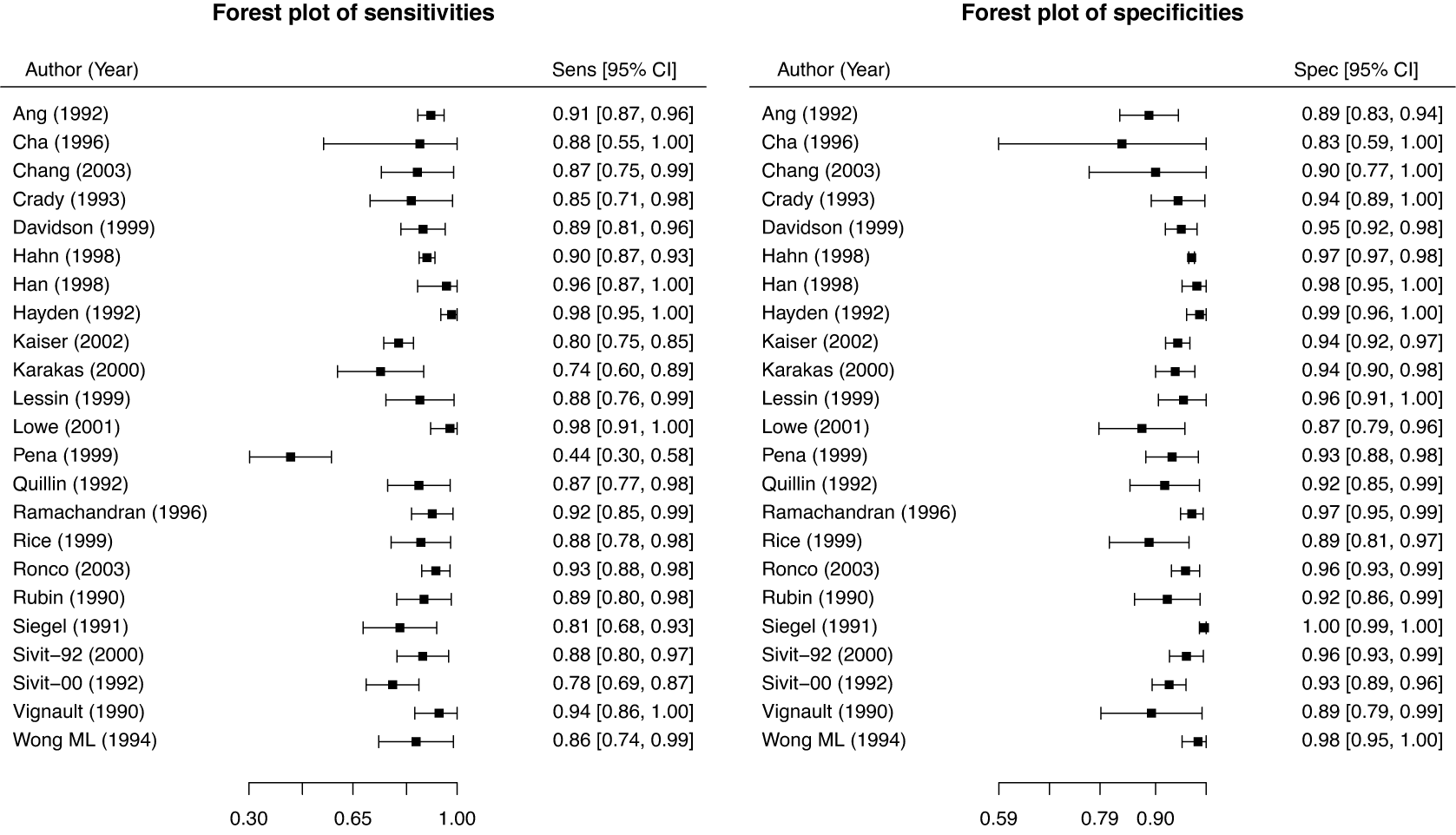
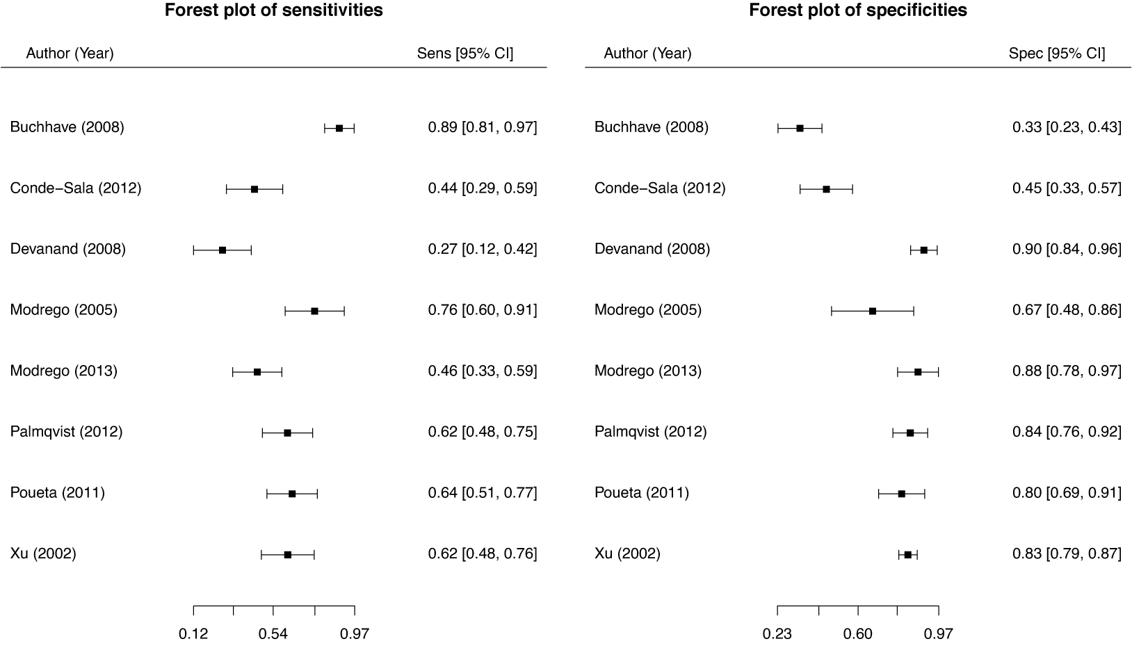
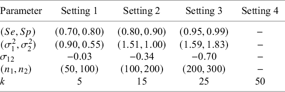
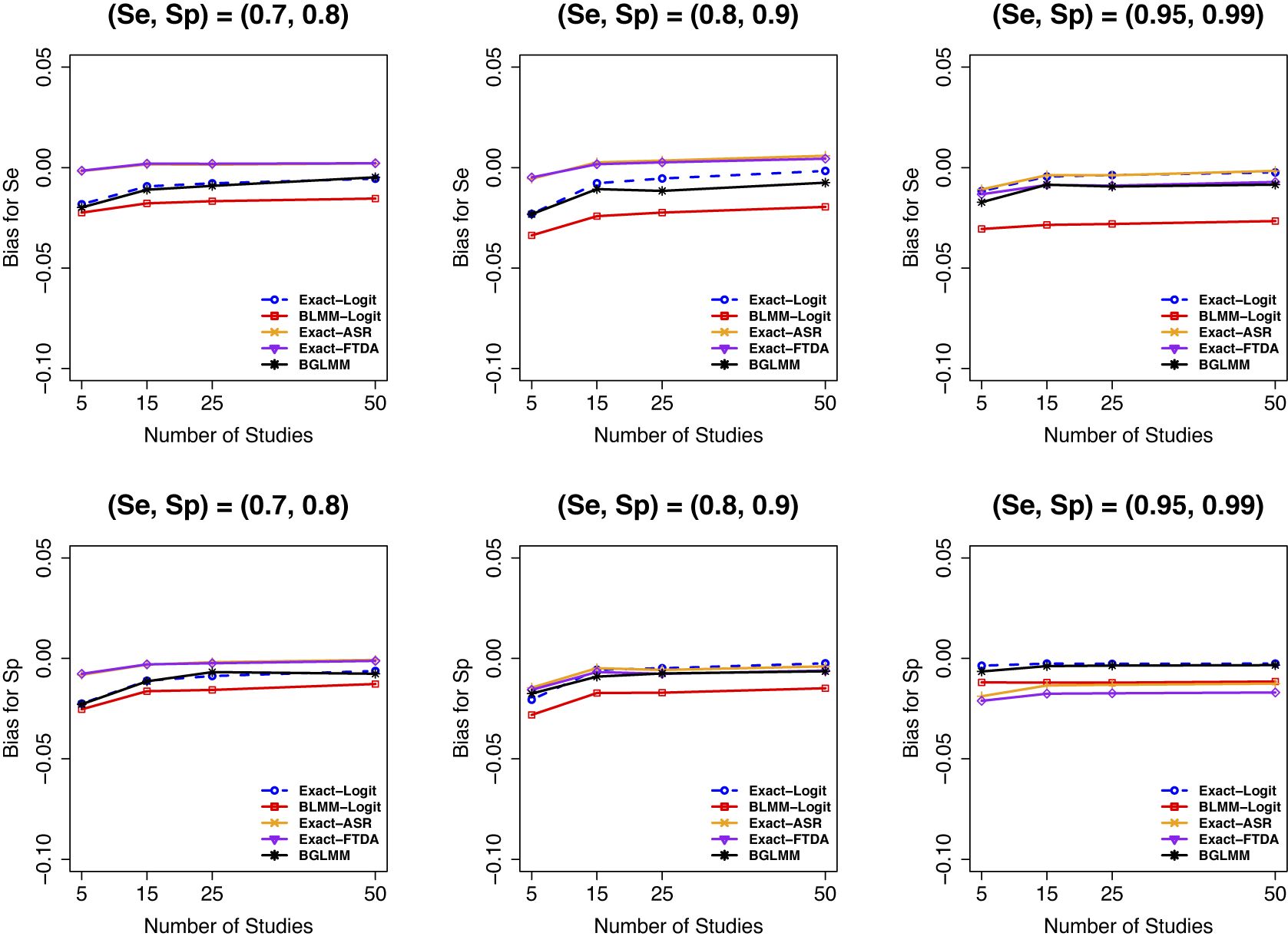


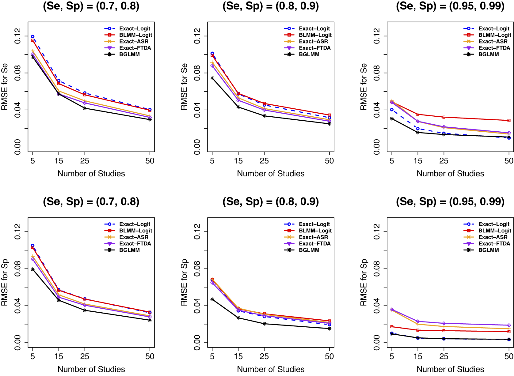


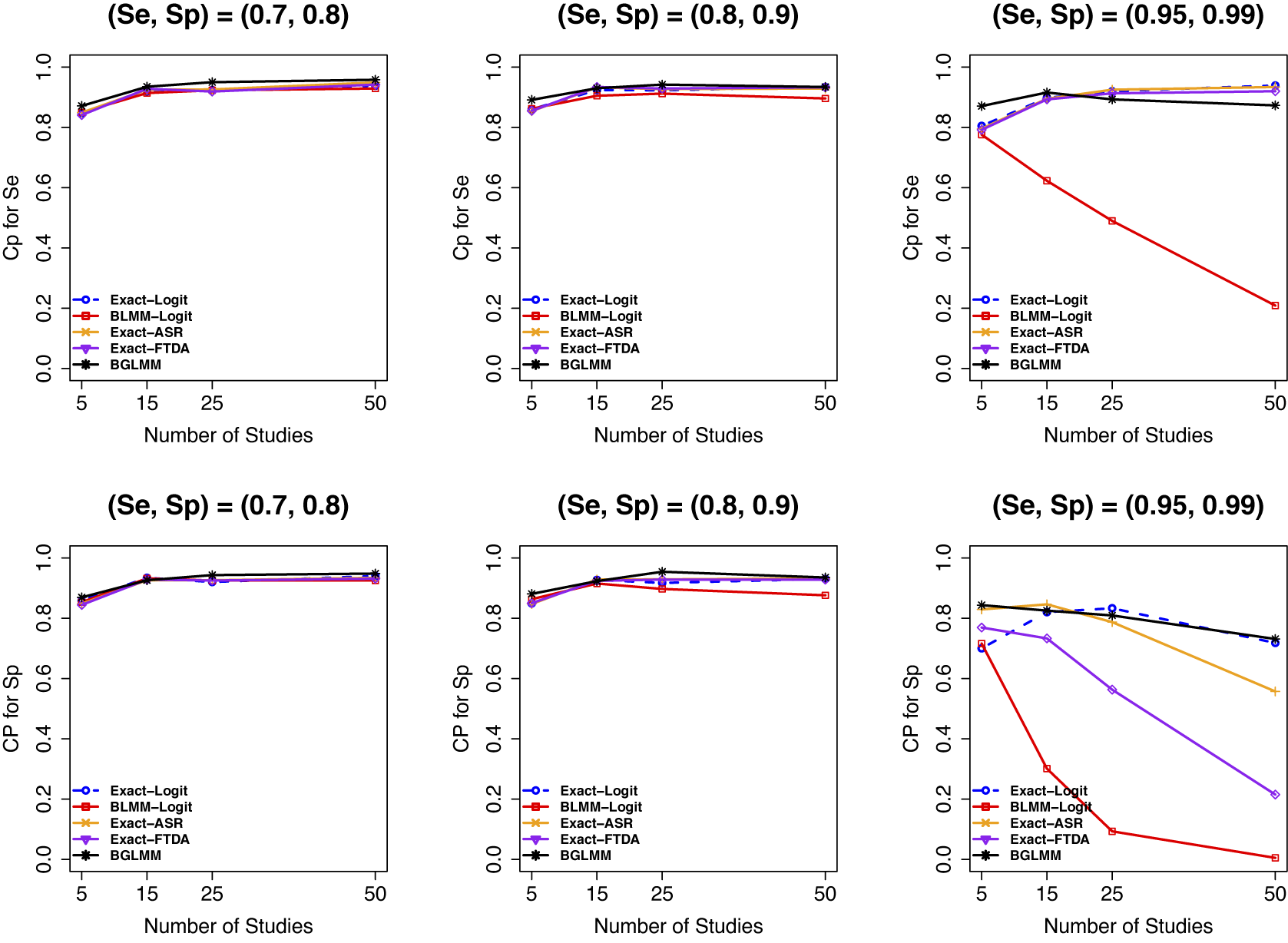


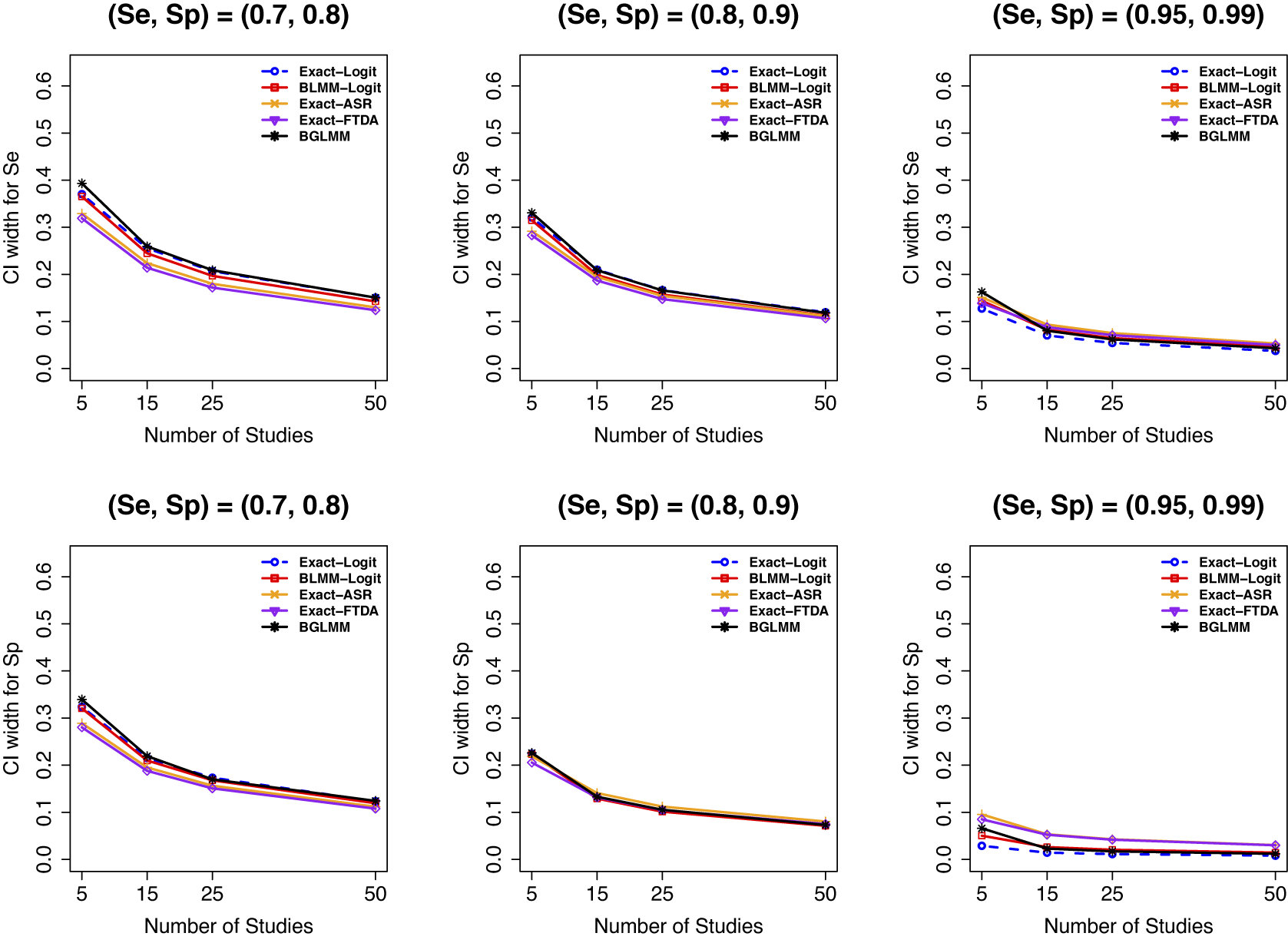


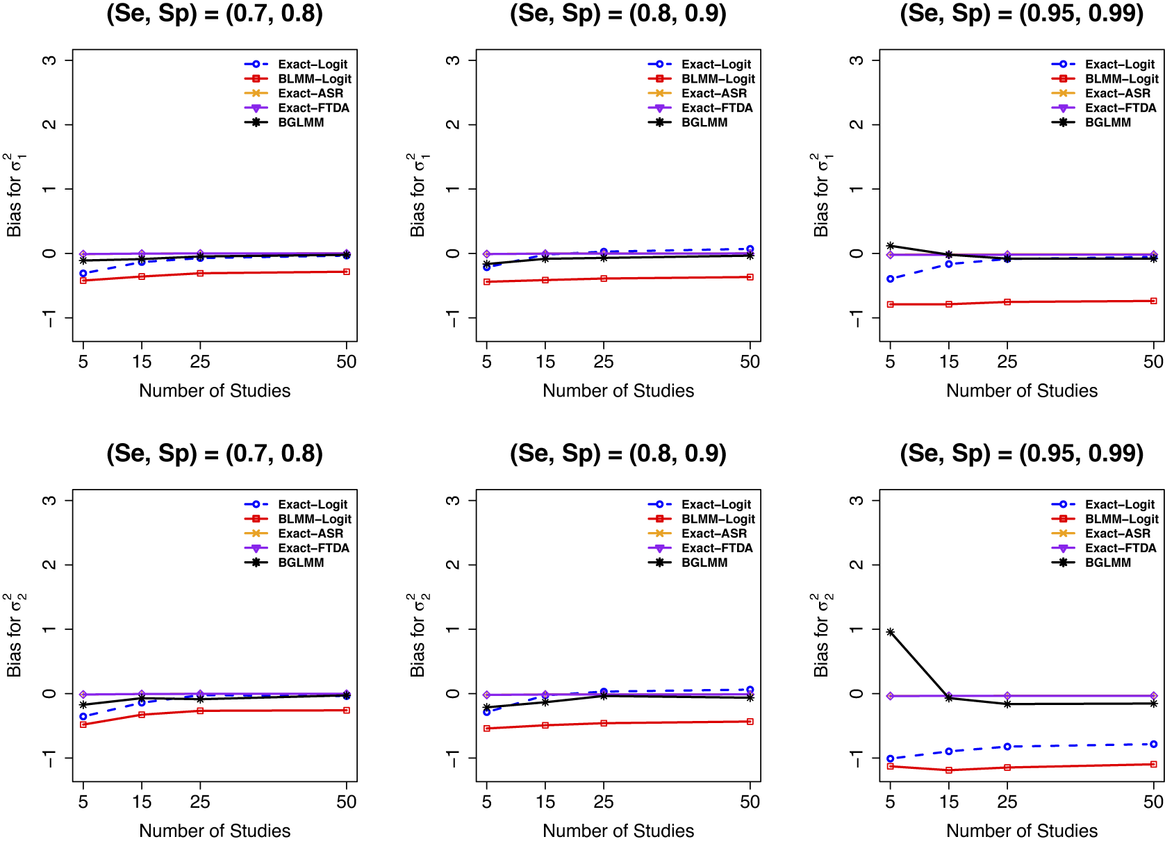


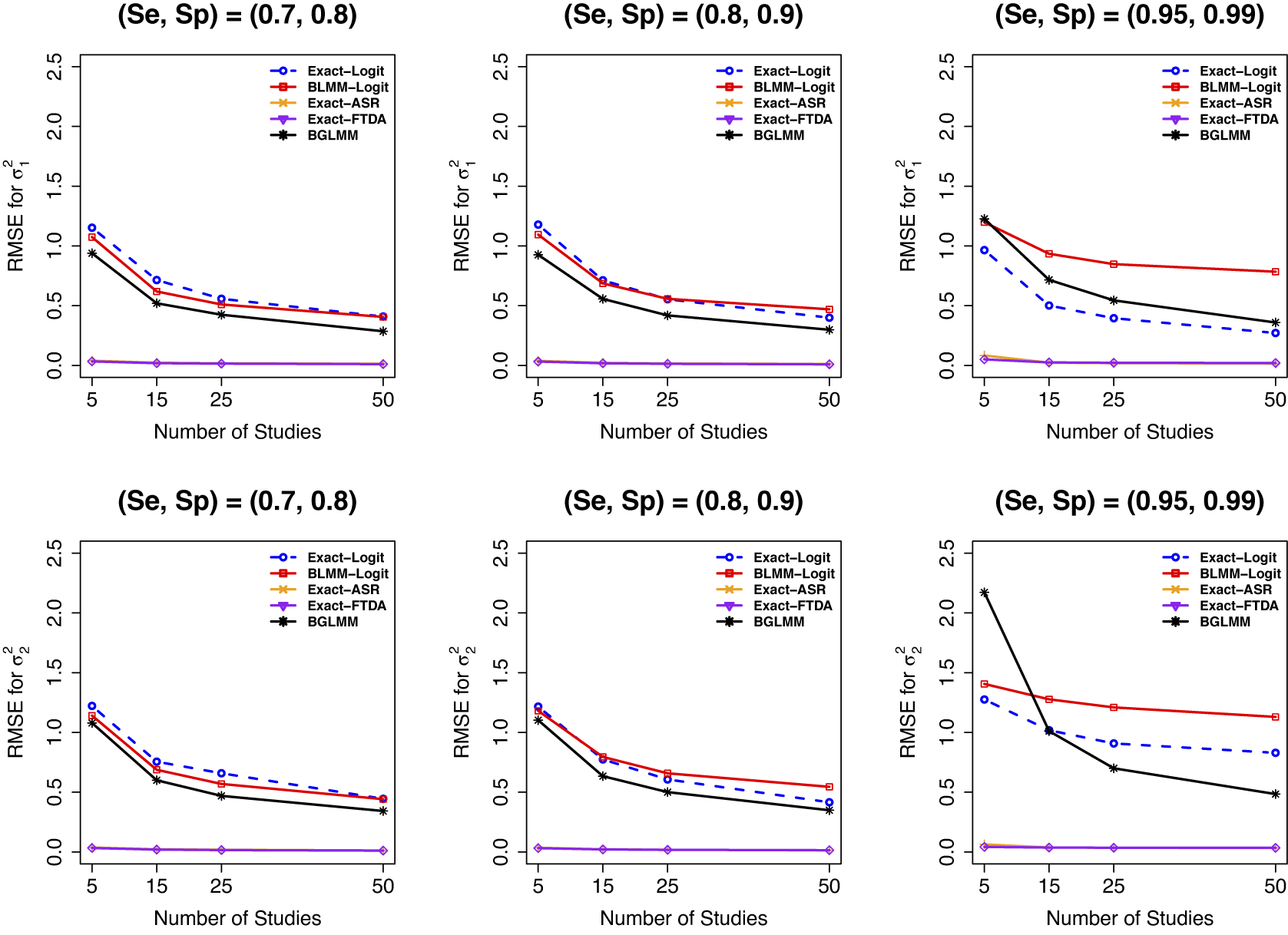


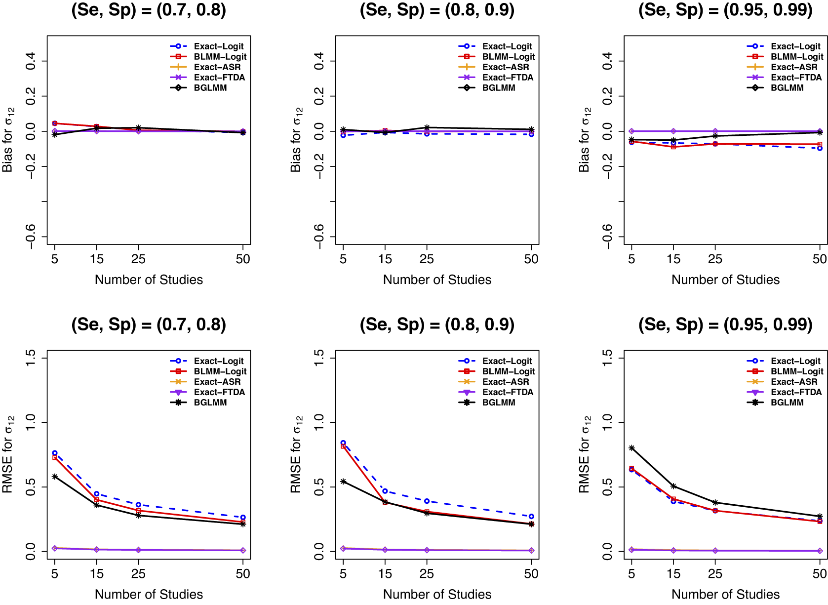


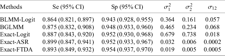
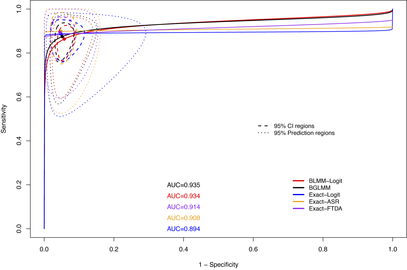
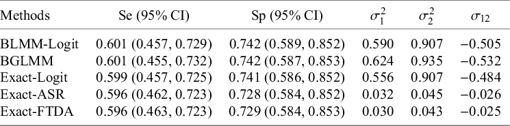
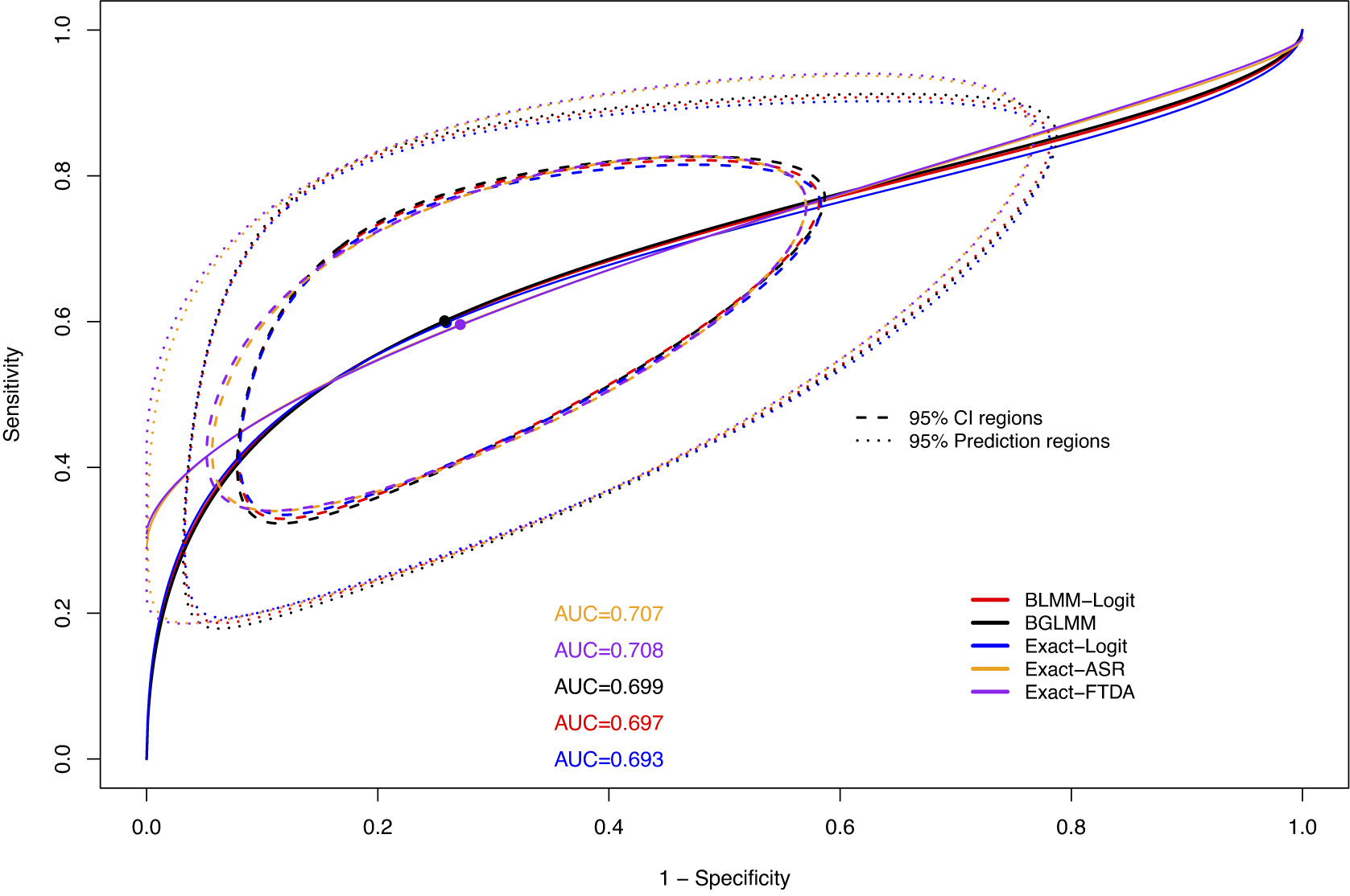


 Open access