Conditional relationships in dynamic models

Abstract

Many political science theories posit empirical relationships that are conditioned by some moderating variable, which scholars model using a multiplicative interaction term in a regression. In recent years, scholars have begun using such terms in dynamic regression models with time series data. However, the lack of guidance on adding multiplicative interactions to these workhorse models exposes problems with the consistency of the estimator, model restrictions, and interpretation. This paper provides theoretical and practical guidance to address these problems. First, we define the conditions under which scholars can ensure consistent estimates when estimating relationships conditioned by a moderating variable in dynamic models. Second, we introduce a general model that makes no theoretical assumptions about precisely how conditional relationships unfold over time. Third, we develop a flexible approach for interpreting such models. We demonstrate the advantages of this framework with simulation evidence and an empirical application.

Scholars are increasingly interested in relationships that suggest the effect of an independent variable, $x$, on a dependent variable, $y$, is conditioned on a moderating variable, $z$ (Brambor et al., 2006; Hainmueller et al., 2019). With an abundance of datasets to test such theories, many scholars are turning to dynamic models—which allow the effect of a covariate on the response to change over time—because they yield estimates of long-run effects. For example, Nooruddin and Simmons (2006) find that International Monetary Fund programs reduce social spending most sharply in democracies, while Kono (2008) considers the effect of democratization on trade liberalization, conditional on the wealth of the trading partners. Similar applications have contributed to a variety of literatures across the discipline.¹

These models are often intuitive representations of complex systems of variables. Yet even for workhorse specifications such as autoregressive distributed lag and error correction models (ADLs and ECMs, respectively),² there is little guidance on how best to model these multiplicative interaction terms. As a result, scholars’ findings are vulnerable to three problems:

1. (1) Estimation. A large literature describes how scholars can ensure that ADLs are appropriate for their data through extensive “pretesting,” particularly by examining stationarity and cointegration (e.g., Philips, 2018). However, it is unclear what tests an interaction term must satisfy, so scholars may not be able to guarantee that ordinary least-squares (OLS) will produce consistent estimates.

2. (2) Specification. Typically, each variable of interest in an ADL suffers from some amount of autocorrelation: its present value is a function of its past values. Choosing which lagged values to include in the model generates different statements about how the researcher believes covariates affect the response over time (Box-Steffensmeier et al., 2014). However, it is unclear what lags of an interaction represent, since either component variable may be lagged, or both. This complication may lead to specifications that imply dynamic effects that differ from what the author intends.

3. (3) Interpretation. ADLs include lags and differences that together allow scholars to interpret their estimates. However, interactions complicate the computation of these quantities, including both short- and long-run effects. Scholars may be unaware of how to derive quantities of interest for their models, potentially leading to incorrect inferences.

This paper aims to help scholars avoid these problems, providing theoretical and practical guidance for studying relationships conditioned by a moderating variable in dynamic models.³ We begin by defining the conditions under which OLS produces consistent estimates: even if two covariates are stationary, their interaction may not be, and so must be explicitly tested for stationarity. Under these conditions, scholars can therefore ensure that OLS is an appropriate estimator simply by extending standard diagnostic procedures.

We then suggest how to specify and interpret a general model with an interaction. We argue that, absent extremely strong a priori beliefs about the data-generating process (DGP), scholars should proceed from a specification that allows covariates to interact freely across time. We introduce such a model that includes all possible cross-period interactions; two variables, each with $p$ lags, generates $(p+1)^2$ interaction terms that capture a single conditional relationship. We use Monte Carlo simulations to examine the tradeoffs of this approach: namely whether the risk of overfitting that comes along estimating a general model with $(p+1)^2$ interaction terms⁴ is outweighed by the potential for bias that arises from invalid restrictions. We find that the flexible approach introduced here produces more reliable inferences: while there is some evidence of overfitting, this risk is relatively minimal compared to the potential bias in estimates resulting from an invalid restriction on the model. Finally, we illustrate how these findings contribute to more robust inferences with an empirical application from Cavari (2019).

1. Ensuring consistent estimates

There are many ways of modeling dynamic dependence among variables. Due to space constraints, we only study multiplicative interactions in ADLs, since they are the most common conditional relationships in the most common time series models in political science (Box-Steffensmeier et al., 2014).⁵ Furthermore, we assume throughout that scholars have carefully investigated whether an interaction is theoretically justified.

The ADL can be written in its general form as

(1)\begin{equation} y_t = \alpha_0 + \sum_{f=1}^p\alpha_fy_{t-f} + \sum_{g=0}^q\beta_{g}x_{t-g}+\epsilon_t . \end{equation}

This specification is ADL( $p$, $q$), with $p$ lags of $y_t$ and $q$ lags of $x_{t}$ (and additional covariates as needed). The standard approach to modeling these relationships is based on Hendry (1995) and the general-to-specific modeling strategy, with the inclusion of a general number of $p$ and $q$ lags that are pared down with the goal of ensuring that $\epsilon_t$ is “white noise,” with $\mathbb{E}$( $\epsilon_t$, $x_{g,t-h}$) $~=0 ~\forall~ t$, $g$, $h$ (see Linn and Webb, 2020; Vande Kamp and Jordan, 2025).

A precondition to using the general-to-specific modeling framework is equation balance: the covariates on the right-hand side of the model are collectively of the same order of integration as the outcome variable (and that this model can be expressed such that the outcome variable is itself stationary). Equation balance can be achieved if all variables are differenced until stationary; such an approach is typically used when applying the ADL model.⁶ To ensure that their models meet this condition, scholars should adopt the two-step balance test procedure proposed by Pickup and Kellstedt (2023)—interrogate the theory to examine whether equation balance is theoretically plausible, and then test the balance properties of the model prior to estimation.

Scholars are hopefully accustomed to testing for such properties in their existing ADL models, but no process or advice extends this testing to models with multiplicative interaction terms. While it seems intuitive that the “memory” of an interaction of two variables would directly follow the properties of the variables themselves, this relationship does not always hold, and the standard practice of diagnosing the time-series properties of all lower-order terms cannot guarantee consistent OLS estimates. For the first time, we provide theoretical results establishing when OLS estimates are consistent for a model with an interaction and how to test for those conditions.⁷ We begin with the most basic case, in which all variables, including covariate $x$ and a moderating variable $z$ (the standard notation in the literature of independent variables that are interactive) are stationary. By definition, this case requires that interaction terms are also themselves stationary. Proposition 1.1 specifies where this holds.

Proposition 1.1. Assume $x$ and $z$ are covariance-stationary autoregressive stochastic series. A series $xz$ composed of their multiplicative interaction is itself stationary if and only if $\mathbb{C}[x_{t}^{1+a},z_{t}^{1+b}] = f(a, b)$ and $\mathbb{C}[x_{t}x_{t+\ell}^{c},z_{t}z_{t+\ell}^{d}] = f(c, d)$ where $t, \ell \in \mathbb{Z}_{\geq0}$, and $a, b, c, d \in \{0,1\}$.

Some of the conditions implied by Proposition 1.1 are easy to understand. The covariance between the two constitutive terms ( $\mathbb{C}[x_{t},z_{t}]$) cannot be a function of time; neither can the covariance of their squares ( $\mathbb{C}[x_{t}^{2},z_{t}^{2}]$) nor the covariance of a constitutive term and the square of the other constitutive term ( $\mathbb{C}[x_{t},z_{t}^{2}]$, $\mathbb{C}[x_{t}^{2},z_{t}]$). Other terms are more difficult to interpret, such as $\mathbb{C}[x_{t}x_{t+\ell},z_{t}z_{t+\ell}]$, but also must not be a function of time. The overarching conclusion, however, is that the product of two stationary series is not necessarily stationary itself due to the possibility of their covariation changing over time. Furthermore, this result indicates that a balanced equation may become unbalanced when an interaction is added to it.

Practically, Proposition 1.1 suggests that scholars always need to explicitly test interaction terms for stationarity. This result can be made more intuitive by considering a special case in which stationarity is guaranteed to hold: when the two variables are stochastically independent.

Corollary 1.2. Assume $x$ and $z$ are covariance-stationary autoregressive stochastic series. If $x$ and $z$ are stochastically independent, a series $xz$ composed of their multiplicative interaction is itself covariance-stationary.

Stochastic independence is a difficult assumption for two observed time series. But scholars are increasingly interested in performing experiments with time series data (Bojinov and Shephard, 2019; Bojinov et al., 2021). Were a scholar to perform a time series experiment and then check to see if the treatment effect is conditioned by an observed moderator, the product of the treatment and the moderator would be stationary if the moderator itself were stationary. Generally, scholars should pretest interaction terms directly to be sure that they are stationary (and that they do not upset equation balance).

An example helps illustrate how this problem might arise in practice. Suppose two variables are known to be stationary, but their correlation is a function of time, as in a Dynamic Conditional Correlations (DCC) framework. Such relationships are common, for instance, with variables such as economic growth and presidential approval (Lebo and Box-Steffensmeier, 2008). Although each variable would pass stationarity tests individually, their interaction may be nonstationary, and OLS estimates for a model that includes this interaction may be inconsistent. This scenario is a straightforward example of the spurious regression problem, a well-understood and widely documented phenomenon (Yule, 1926; Grant and Lebo, 2016). On one hand, the result in Proposition 1.1 adds to the already-substantial burden on researchers to pretest their data. On the other hand, however, pretesting each variable for stationarity is standard practice in time series modeling. There are a number of tests that have been developed and implemented across statistical software for this purpose (see Box-Steffensmeier et al., 2014, for a recent review).⁸ These same tests can be used for interaction terms.

Proposition 1.1 establishes that ADLs are appropriate models of relationships conditioned by a moderating variable in dynamic systems, so long as scholars extend the standard diagnostic procedures to include interaction terms.⁹ These results speak only to consistency, not the other desirable properties, of OLS estimates. In addition, it gives no advice on the structure of an underlying interactive model: we suggest such a general model in the next section.

2. Specifying relationships conditioned by a moderating variable

Despite a large literature on the properties of ADLs, scarce attention is paid to specifying relationships of interest, other than the general-to-specific advice alluded to previously. This lacuna is unfortunate, as even small variations among relatively simple models can imply very different dynamics. Virtually no advice exists for specifying conditional relationships, potentially leading to incorrect or incomplete models and interpretations. We fill this gap by suggesting a general interactive model, inspired by the tradition of the general-to-specific modeling strategy, and introducing key quantities of interest for its interpretation.

2.1. The general interactive model

Following the spirit of the general-to-specific model, a general starting point is a model that allows a covariate interaction to unfold freely across time. A general ADL model will allow the data to determine the structure of effect moderation; that is to say, the data should be allowed to determine whether multiplicative interactions include cross-lags. An ADL( $p$, $q$) model of the most general form with a multiplicative interaction is:

(2)\begin{equation} y_t = \alpha_0 + \sum_{f=1}^p\alpha_{f}y_{t-f} + \sum_{g=0}^q \beta_{g}x_{t-g} + \sum_{h=0}^q \theta_{h}z_{t-h} + \sum_{g=0}^q\sum_{h=0}^q \zeta_{g, h}x_{t-g}z_{t-h} + \epsilon_t . \end{equation}

In political science, most long-term dynamic processes can be captured by first-order dynamics. As such, we focus our attention on an ADL(1,1) model that includes a general specification for a multiplicative interaction:

(3)\begin{align}y_t &= \alpha_0 + \alpha_1y_{t-1}+\beta_0 x_t + \beta_1 x_{t-1} + \beta_2 z_t + \beta_3 z_{t-1} + \nonumber \\ &\qquad \qquad \beta_4 x_t z_t + \beta_5x_{t-1}z_t + \beta_6x_t z_{t-1} + \beta_7 x_{t-1}z_{t-1} + \epsilon_t .\end{align}

Because this ADL(1,1) model features one lag of the independent and moderating variables, it features the multiplicative interaction $x_{t}z_{t}$ and its lag $x_{t-1}z_{t-1}$. To ensure there are no restrictions on this moderated relationship, however, a general model will also include $x_{t-1}z_{t}$ and $x_{t}z_{t-1}$. Specifying a conditional relationship, therefore, requires $2 \times 2$ interaction terms in addition to the lower-order variables. More generally, a multiplicative interaction in a general ADL( $p$, $q$) model generates $(q + 1)^2$ new parameters, which allows the covariates to interact across any points in time.¹⁰ These terms all appear in calculating quantities of interest; eliding any implies a restriction on the dynamic system.

This specification is a reasonable starting point for most applications. For one, the cost of invalid parameter restrictions is enormous: biased estimates and incorrect inferences (De Boef and Keele, 2008). Erroneously constraining any of the $\beta$ or terms in the general model to zero breaks the link between different periods of the same variable. Failing to account for the “memory” of each process in this way induces bias not only for the covariate directly constrained, but also among any interacted variables and lower-order terms. For instance, setting $\beta_4 = 0$ when it is non-zero in the true DGP biases estimates of all $xz$ terms, and through the conditional relationship, all $x$ and $z$ terms (that is, it biases all $\beta$ terms in Equation 3). The logic of this starting point also mirrors the common advice to include all of an interaction’s constitutive terms in modeling applications (e.g., Brambor et al., 2006; Clark and Golder, 2023). The Monte Carlo exercise below underscores the magnitude of these problems: in some cases, invalid restrictions can produce essentially random estimates.

This general model is also attractive because it privileges information in the data over broad theoretical intuition. Even the most precise theories are generally silent on exactly when covariates interact, so a conservative approach is to allow for all possibilities. Moreover, where theory does provide such strong guidance on the timing of the interaction, these hypotheses can be empirically tested by estimating the general model. Rather than impose restrictions based on a priori beliefs, this approach allows scholars to treat parameter estimates as evidence of how the dynamic system behaves.

A final advantage of this model is that it allows scholars to parse different components of a single conditional relationship. The interaction $xz$ can vary because of a shift in $x$ alone, $z$ alone, or both. By estimating all cross-period interactions, scholars can study the effect of each change on the dependent variable separately. All of these features contribute to a richer set of inferences.

2.2. Interpreting the general interactive model

Quantities from such a general model might seem challenging to calculate or interpret. In the following, we demonstrate this is not the case, providing formulae on how to calculate typical quantities of interest like short-run effects and long-run multipliers (LRMs). We additionally give examples of these calculations through our replication example.

Scholars studying dynamic models are usually interested in change in the response $y$ as a function of change in (or “shock” to) a variable $x$. The typical quantities of interest are period-specific effects and cumulative effects.¹¹ Period-specific effects are defined as the change in $y$ at any time as a result of a shock to $x$ at time $t$. In other words, they answer: “what will happen to the response at some future date if a covariate shock occurs today?” For any period $t+j$, where $t$ and $j$ are integers, this quantity can be calculated by specifying the model for $y_{t+j}$ and differentiating with respect to $x_t$. From Equation 3, note that

\begin{align*} y_t &= \alpha_0 + \alpha_1y_{t-1} + \dots, \\ y_{t+1} &= \alpha_0 + \alpha_1y_{t} + \dots, \\ &\enspace \vdots \\ y_{t+j-1} &= \alpha_0 + \alpha_1y_{t+j-2} + \dots, \\ y_{t+j} &= \alpha_0 + \alpha_1y_{t+j-1} + \dots, \end{align*}

so that each expression can be substituted for the next period’s lagged $y$.¹² Thus, we can start in period $t+j$ and recursively substitute previous periods of $y$ until the right side of Equation 3 appears. Scholars typically restrict attention to the case where $j=0$, which De Boef and Keele (2008) refer to as the “short-run effect”: a particular period-specific effect for the first period $j=0$ only.¹³ Differentiating with respect to $x_t$ therefore yields the expression for the short-run (or instantaneous) effect:

(4)\begin{equation} \frac{\partial y_{t}}{\partial x_t} = \beta_0+\beta_4z_t + \beta_6z_{t-1} \end{equation}

The second quantity of interest, often the motivation for studying such models, is cumulative effects. These effects, which provide information about relationships over time, can be calculated by summing period-specific effects. There is one special case of a cumulative effect that receives the majority of scholarly attention: the total change in $y$ resulting from a change in $x$. This quantity is known as the long-run effect (LRE) or long-run multiplier (LRM):¹⁴ the total change in $y$ after an infinite number of periods

(5)\begin{equation} \sum_{j=0}^\infty \dfrac{\partial y_{t+j}}{\partial x_t} = \frac{\beta_0 +\beta_1 + \beta_4z_t + \beta_5z_{t+1} + \beta_6z_{t-1} + \beta_7z_t}{1-\alpha_1} . \end{equation}

This derivation demonstrates that the LRM is more precisely the total cumulative effect, since it maximizes the window over which change in $y$ is summed. Scholars can use these quantities of interest to fully interpret the general interactive model we propose.¹⁵ It is also readily apparent why the calculation of these quantities of interest differ in the general interactive model versus a model without the fully specified cross-period interactions. If we only included the contemporaneous interaction $x_tz_t$, Equation 4 would omit $\beta_6z_{t-1}$ (or, more generally, any $\beta_j$ that contains a term in which $x$ appears contemporaneously), and Equation 5 would potentially omit all of $\beta_5z_{t+1}$, $\beta_6z_{t-1}$, and $\beta_7z_t$. Our Monte Carlo simulations show that such omissions clearly alter the effect estimates. Calculation of standard errors for these effects can be done using standard methods. The short-run effect is a linear combination of coefficients and, as such, standard errors can be calculated exactly. The long-run effect is a nonlinear combinations and, as such, standard errors must be approximated using either parametric bootstrapping or the delta method. We rely on the former method, while noting that scholars can feel free to use the latter if they so choose.

The general model proposed here is consistent with a widely accepted, general-to-specific modeling framework. It is agnostic about the dynamic nature of the underlying interaction, allowing a conditional theory to be tested without strong parameter assumptions. And it is straightforward to interpret. Yet as Grant and Lebo (2016) note, increasing the number of covariates exacerbates bias for the parameter relating to the lagged response ( $\alpha_1$, or the error correction rate [ECR], which determines the persistence and decay of effects of independent variables in dynamic models that contain lagged dependent variables). Since the ECR is present in all calculations of dynamic effects, adding interactions may threaten inferences about long-term relationships among variables. Furthermore, there is much less information in time series data than sample sizes suggest, making it likely that scholars who add extra covariates are simply modeling noise (or “overfitting”) (Keele et al., 2016). ECR bias and overfitting are important problems that scholars need to grapple with as they study dynamic models, and there is no clear consensus on how to avoid them, other than to keep models simple. We take up these concerns in the context of our proposed interactive model in the simulation analysis below.

3. Simulation evidence

The general model might have attractive features in the abstract, but its performance remains to be seen. We assess this performance using Monte Carlo simulations to answer four questions: (1) whether the fully interactive model better estimates the parameters of interest, (2) whether this comes at the cost of overfitting, (3) whether “typical” time series have the statistical size to adequately estimate such a model, and (4) whether these general costs are outweighed by the benefits of estimating a general model. If the benefits of fitting a general model are outweighed by these problems, then scholars may wish to study less complex models with implicit parameter restrictions instead. We first simulate data from four DGPs—one with no exogenous predictors, one with two predictors $x$ and $z$ but no interaction, one with a contemporaneous-period only (“restricted”) interaction between $x_t$ and $z_t$, and one with the general (“fully interactive”) model from Equation 3 in the previous section. Through this section, each DGP is identified by a short label:

(LDV)\begin{equation} y_t = \rho_y y_{t-1}+\eta_{y,t} , \end{equation}

(No interaction)\begin{equation} y_t = \alpha_0 + \alpha_1y_{t-1}+\beta_0 x_t + \beta_1 x_{t-1} + \beta_2 z_t + \beta_3 z_{t-1} + \epsilon_t , \end{equation}

(Restricted)\begin{equation} y_t = \alpha_0 + \alpha_1y_{t-1}+\beta_0 x_t + \beta_1 x_{t-1} + \beta_2 z_t + \beta_3 z_{t-1} + \beta_4 x_t z_t + \epsilon_t , \end{equation}

(Full interaction)\begin{align} y_t &= \alpha_0 + \alpha_1y_{t-1}+\beta_0 x_t + \beta_1 x_{t-1} + \beta_2 z_t + \beta_3 z_{t-1} + \nonumber \\ &\qquad \qquad \beta_4 x_t z_t + \beta_5x_{t-1}z_t + \beta_6x_t z_{t-1} + \beta_7 x_{t-1}z_{t-1} + \epsilon_t , \end{align}

where $x_t = \rho_x x_{t-1} + \eta_{x,t}$ and $z_t = \rho_z z_{t-1} + \eta_{z,t}$. We hold the $\alpha$ and $\beta$ terms fixed across all simulations. For each of the DGPs, we examine $3^4 = 81$ cases, varying the time series length $n \in \{50,100,500\}$ and the autoregressive parameters $\rho_x, \rho_z, \rho_y \in \{0.1,0.5,0.9\}$. For each of the 324 $(4 \times 81)$ experimental conditions, we create 500 datasets, with each variable’s starting value and all errors ( $\epsilon, \eta_x, \eta_z, \eta_y$) drawn from $\mathcal{N}(0,1)$. We then estimate three models (the no interaction, restricted, and fully interactive [general] models) and store the results.

Turning first to the question of ECR bias, Figure 1 presents clear evidence that the general model does not produce worse estimates of $\alpha_1$ than does a simpler model. The top panel plots estimates from the model without any interaction terms (in triangles), the restricted model with just $x_tz_t$ estimated (squares), and the general model (circles), for each of the four DGPs. Each point represents the median estimate across 500 replicates under the same experimental condition, with dashed lines for the true values (each $\rho_y$ in the LDV DGP, and $\alpha_1 = 0.5$ for the others). Even when fit to a DGP with no conditional relationships, the general model provides estimates at least as close to the true value as those of a simpler model (the far-left column); the general model dominates the DGP includes a complex conditional relationship (the far-right column). This performance is reflected in Table 1, which presents median absolute ECR bias ( $\lvert \hat{\alpha}_1-\alpha_1\rvert$ calculated for each replicate), averaged across all conditions under each DGP. Overall, the general model produces the lowest absolute bias.

Figure 1. Monte Carlo simulation results for the error correction rate, $\alpha_1$. Triangles represent estimates from the model without an interaction, squares are from a restricted model, and circles are from the general model. Median estimates are plotted against the true values (dashed lines) in the top panel. The bottom panel plots the mean proportion of 500 replicates under each condition for which $95\%$ confidence intervals contain the true value.

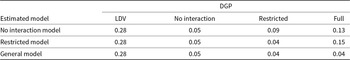
Table 1. Average absolute bias, $\hat{\alpha}_1$

The bottom panel of Figure 1 plots coverage probabilities for estimates of $\alpha_1$—the proportion of the 500 replicates under each condition for which the $95\%$ confidence interval (constructed via parametric bootstrap) for $\hat{\alpha}_1$ contains the true value.¹⁶ Again, the evidence suggests that the general model recovers better estimates of the ECR, with higher coverage probabilities across the board than those of simpler specifications. Across all conditions, the mean coverage rate for the general model is $93\%$, very close to the $95\%$ rate predicted by theory and much better than the $79\%$ and $81\%$ rates for the no interaction and restricted models, respectively. Even when we ignore the full interaction DGP—the most favorable case for the general model—the coverage rate ( $93\%$) remains as accurate as that of the restricted model ( $93\%$) and higher than the no interaction model ( $87\%$). On question (1): these data suggest that across a broad range of experimental conditions, the fully interactive model better estimates the ECR parameters of interest, both by lowering the bias when the DGP is conditional as well as not exacerbating ECR bias when the DGP is not conditional.

We turn now to overfitting: whether the introduction of a surplus of parameters to estimate induces the model to account for random noise or error rather than the underlying relationship (Keele et al., 2016, p. 32). Here, the risk is that the general model uses related parameters (like the cross-period interactions) to fully model the interaction. If this problem were severe, we should see (1) worse out-of-sample predictive power for the general model, relative to more parsimonious specifications, and (2) higher Monte Carlo variance (i.e., unstable coefficient estimates) across replicates under the same experimental condition.

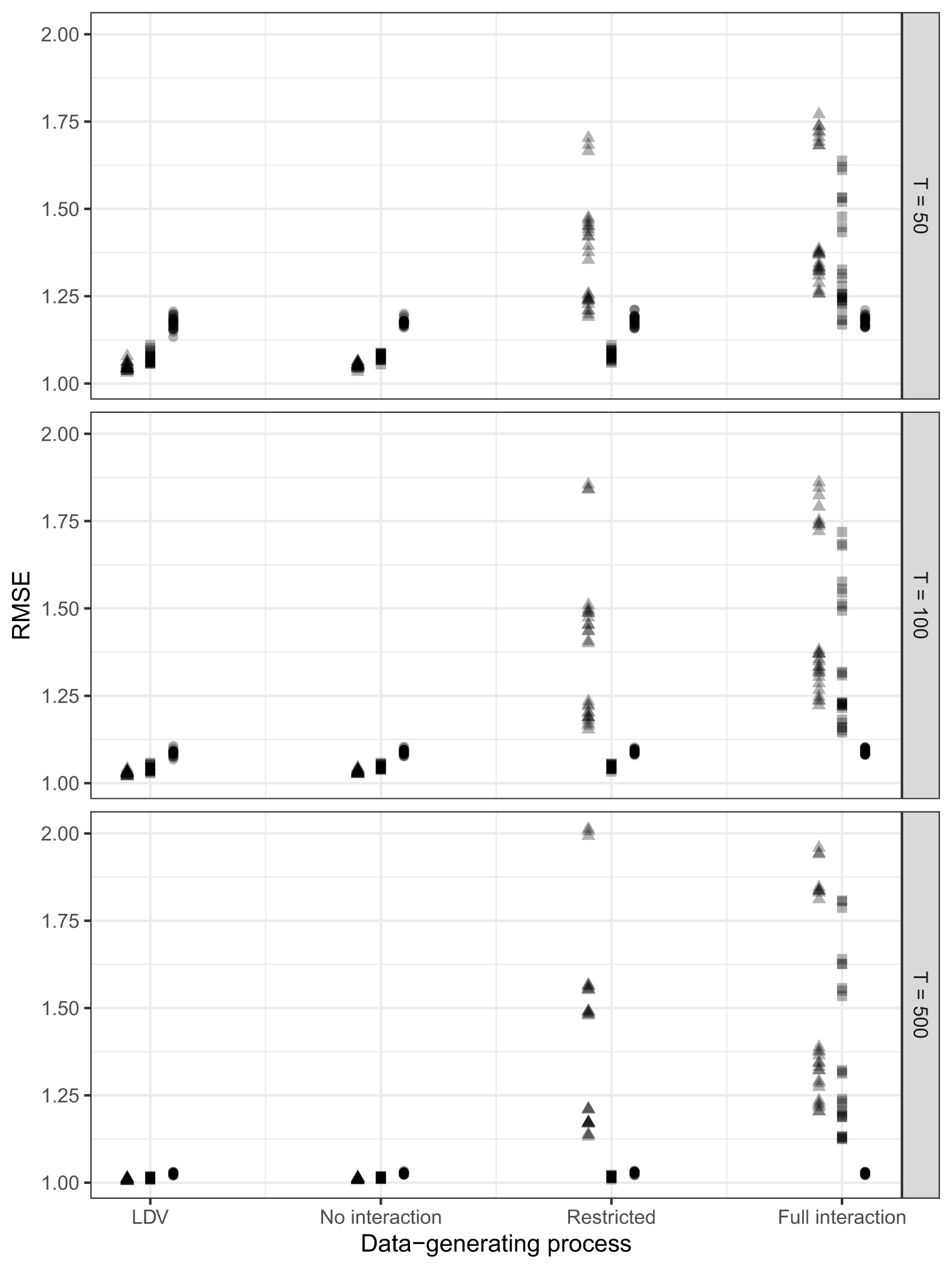
Figure 2 plots the median root mean squared error (RMSE) for out-of-sample predictions generated through 5-fold cross-validation (a common method for measuring the typical deviation of an estimate from a parameter’s true value).¹⁷ All models perform better with longer time series, consistent with existing scholarly evidence, with RMSEs 10-25 $\%$ smaller under $T=500$ compared to $T=50$. With short time series and no interaction in the DGP, the general model produces RMSEs about 5-15 $\%$ larger than those of simpler specifications. However, where there is an interactive process in the DGP, simpler specifications produce RMSEs approximately 25-75 $\%$ larger than those of the general model—and this effect does not diminish as sample size increases. Most importantly, the restricted model (squares) does not obtain markedly better predictive power than the general model (circles), even when applied to a restricted interaction DGP.

Figure 2. Monte Carlo simulation results for RMSE from 5-fold cross-validation. Triangles represent RMSE from the model without an interaction, squares are from a restricted model, and circles are from the general model. The top panel is for a time series of length $T=50$, the middle is $T=100$, and the bottom is $T=500$. Each point represents the median RMSE from a 20 $\%$ random sample of each set of 500 replications under each experimental condition.

To compare the stability of estimates across models, Table 2 reports the variance for each set of 500 replicates, averaged across all experimental conditions. The general model has the smallest variance for all parameters except the coefficient on $x_tz_t$, $\hat{\beta}_4$. This result is consistent with slight overfitting, but with a difference of $0.01$, appears to be only a minor concern: the average 95 $\%$ quantiles of $\hat{\beta}_4$ for each set of replicates has a width of 0.45 for the general model, compared to 0.31 for the simple interaction model. On question (2): the RMSE and variance evidence suggest that overfitting is a relatively minor concern for the general model.

Table 2. Mean Monte Carlo variance across all simulations

We turn next to the question of size. The general, fully interactive model is quite complex and encourages the estimation of a considerable number of parameters. The evidence above assumes a minimum time series length of $T = 50$: are shorter time series up to the task? To answer, we additionally simulate the same DGPs, but with $T = 15$. Figure 3 combines the same evidence from Figures 1 and 2. In the top panel are the ECR estimates for $T = 15$. We observe that, as expected, all models perform uniformly worse under such data constraints. The fully interactive model, though, suffers no unique problems: when the DGP is only the LDV, or not interactive, or the “restricted” interaction, the general model performs as well as other models. If the DGP is fully interactive, the fully interactive model performs best (far-right column), even given the number of parameters it needs to estimate.

Figure 3. Monte Carlo simulation results for the error correction rate, $\alpha_1$, and RMSE from 5-fold cross-validation for short ( $T = 15$) time series. Triangles represent estimates from the model without an interaction, squares are from a restricted model, and circles are from the general model. Median estimates are plotted against the true values (dashed lines) in the top panel. The middle panel plots the proportion of 500 replicates under each condition for which $95\%$ confidence intervals contain the true value. The bottom panel plots the median RMSE from a 20 $\%$ random sample of each set of 500 replications under each experimental condition.

The same is true for ECR coverage. There is noticeably more spread when any model is applied to the LDV data-generating process. Beyond that, the coverage rates are marginally worse than observed in Figure 2, especially when any model is applied to the fully interactive DGP. Even here, though, the general model is the best performer, achieving coverage rates of 85-90%, even with only 15 observations. As expected, however, the issue of overfitting is exacerbated: RMSEs for the fully interactive model are considerably worse than the noninteractive or restricted model. In instances of short time series, scholars might prepare to use the general-to-specific modeling strategy to pare down model parameters. But, overall, on question (3): even in a world of very short ( $T = 15$) time series, the general model provides equally good estimates of parameters of interest, compared to other model specifications, though the general model contains more overall error.¹⁸

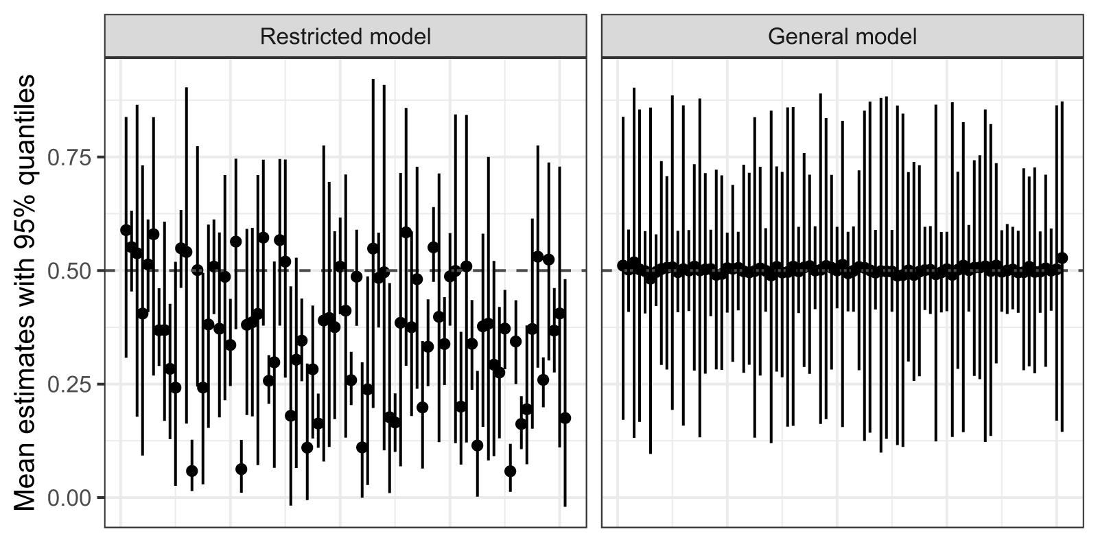
Last is the question of tradeoffs: what are the potential costs of estimating a restricted model? Figures 1 and 2 demonstrate that invalid restrictions on an interactive process (including ignoring it altogether) generate substantial ECR bias, poor coverage rates, and poor predictions. To highlight just one result, inferences about the conditional relationship suffer drastically from invalid restrictions: Figure 4 plots estimates for the coefficient on $x_tz_t$ (the only coefficient estimated by both the restricted and full models) for the restricted and full models (on the left and right, respectively) when the DGP is fully interactive. Each dot represents the median across all 500 replicates within an experimental condition, with lines for 95 $\%$ quantiles. Clearly, mis-specification produces severe bias. Not only are the individual replicates unstable, but so too are their medians, and many 95 $\%$ quantiles completely miss the true value. On question (4): even if there are tradeoffs, the ability to uncover true parameter values mitigates any costs of estimating a general model.

Figure 4. The consequences of invalid restrictions. Monte Carlo simulation results for $\beta_4$ when the DGP includes a complex conditional relationship. Points represent median estimates from 500 replicates of each experimental condition, with lines for $95\%$ quantiles.

Taken together, these results indicate that the cost of estimating a general model is slight—in contrast to the problems that arise from invalid restrictions. These results should give scholars pause, as political scientists almost always study restricted interactive models without comparing them against a more general specification.¹⁹ Our findings indicate that this current standard operating procedure likely produces seriously biased estimates and unreliable inferences: problems easily corrected by a general interactive model.

4. Application: important issues, salience, and presidential approval

To demonstrate how the modeling and inferential framework developed above can improve our understanding of important dynamic relationships, we execute an empirical replication. Cavari (2019) investigates a central problem in public opinion: whether the salience of a political issue affects the relationship between perceptions of the success of an incumbent’s policy and overall approval of that incumbent. A number of studies demonstrate that the U.S. president’s approval ratings can be predicted by perceptions of the president’s handling of important issues, like the economy and foreign policy (e.g., Cohen, 2002). A few studies have further qualified this finding, showing that when media coverage of an issue is high, presidential approval more greatly depends on perceptions of the president’s handling of that political issue relative to other political issues (Edwards et al., 1995, for instance). Cavari intertwines these observations to create a conditional theory of presidential approval: presidents need not be good at all things to maintain their approval, but rather need only to maintain job performance in the issue areas most salient to the public at any point in time.

Cavari tests his theory on a quarterly dataset from 1981-2016, covering the Reagan-Obama administrations. The dependent variable is the percentage of Americans who approve of the way the president is handling his job: classic presidential approval. The key independent variables are “job performance”—approval ratings for the president’s handling of the economy and foreign policy (as separate issue areas)—as well as the salience of those two issue areas to the American public (the percentage of Americans that say that either the economy or foreign policy is the most important political issue). Theoretically, these should interact: job performance in the economy (foreign policy) should matter most when Americans care most about the economy (foreign policy). Cavari also includes controls for macropartisanship, unemployment rate, divided government, and whether it was an election year or the first quarter in a presidential term. Cavari’s preferred model is a first-order partial adjustment model:

\begin{align*} \text{Approval}_{t} &= \alpha_{0} + \alpha_{1}\text{Approval}_{t-1} + \beta_{1}\text{Economic approval}_{t} + \beta_{2}\text{Economic salience}_{t} \,+ \\ &\qquad \qquad \beta_{3}\text{Foreign policy approval}_{t} + \beta_{4}\text{Foreign policy salience}_{t} \\ &\qquad \qquad \beta_{5}\text{Foreign policy approval}_{t}*\text{Foreign policy salience}_{t} + \\ &\qquad \qquad \beta_{6}\text{Economic approval}_{t}*\text{Economic salience}_{t}\, + \\ &\qquad \qquad + \text{Controls}_{t} + \varepsilon_{t} \end{align*}

where Approval is presidential approval, Economic approval is approval of the president’s handling of the economy, Economic salience is the percentage of Americans who think the economy is the most pressing political issue (Gallup’s “Most Important Problem” question), and $\varepsilon$ is a white noise error term. Similar descriptions can be given to Foreign policy approval and Foreign policy salience, but instead focusing on foreign policy. In our view, this model starts with the imposition of potentially invalid restrictions. We do not know a priori if the conditional effects operate in the same period or in different periods (i.e., if performance is important in the same quarter as when the public determines an issue is salient, or if presidents are given a “thermostatic” quarter to acknowledge the public’s priorities and respond to them). The contemporaneous lag structure assumes that both matter in the same period only and that there are no lagged effects.

Of course, our issue is not with Cavari: the author has an interesting, dynamic theory of conditional effects, but is given no clear advice on how to go about modeling them. To echo the above sections, our advice is philosophically consistent with the standard general-to-specific ADL modeling approach: start with a general (interactive) model and, given the results, potentially pare down. To demonstrate the utility of our proposed approach, we begin by testing the stationarity of the constituent interactive terms.²⁰ We find that both salience measures are not stationary. Accordingly, we difference the series and estimate a first-order ADL model that includes lags of all independent variables, including the interactions, as well as the cross-lags (the general model).²¹ Given the number of parameters estimated, we provide model estimates in the Supplemental Materials and focus on graphic interpretations of effects in the main text.

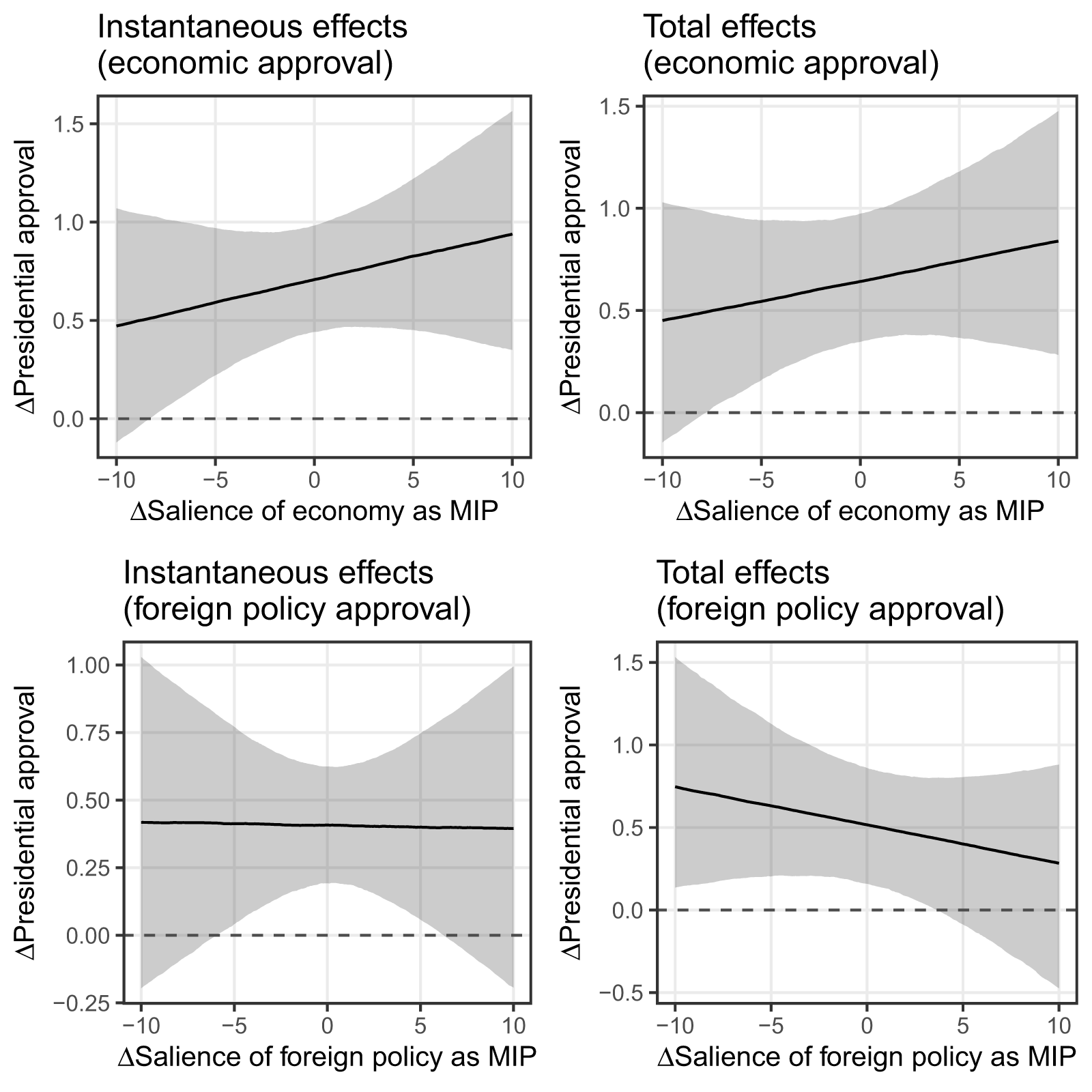
Figure 5 displays the effect of job performance on presidential approval. The top row displays the instantaneous and total effects of economic approval on overall presidential approval; the bottom row for foreign policy approval. The top-left pane shows that, in the short-run, there is a positive, statistically significant relationship between economic approval and overall presidential approval. That effect is conditioned on the salience of the economy: when the salience of the economy jumps in the minds of the public, the relationship between economic approval and overall approval strengthens in magnitude such that presidents can increase their overall approval by about a point when they increase their economic approval by the same amount, as long as salience of the economy is high. The top-right pane shows that the total (long-run) effect of economic approval on presidential approval is almost identical to the instantaneous effect, indicating that there is largely no dynamics in the effect of economic approval on presidential approval.

Figure 5. Dynamic relationship between presidential performance and approval, conditional on salience of the underlying issue. Lines represent predicted instantaneous effects (left) and total effects (right) on presidential approval, holding change in salience its mean value, while varying changes in salience across its observed range. Economic performance is in the top row; foreign policy performance is in the bottom row. Estimates are median estimates from quantiles of 5,000 samples from $\mathcal{N}_{MVN}\left(\hat{\theta},\mathbb{C}(\hat{\theta})\right)$; $95\%$ confidence intervals are shaded in gray.

The bottom row of Figure 5 displays the instantaneous and total effects of foreign policy approval on overall presidential approval. The bottom-left pane shows that, in the short-run, there is a positive, statistically significant relationship between foreign approval and overall presidential approval. That effect is independent of the salience of the issue; regardless of changes to foreign policy approval, the effect is roughly equal to 0.4. In a curious matter, the total effect of foreign policy approval is still positive but appears to be negatively conditioned by the salience of foreign policy: as salience increases, approval of the president’s foreign policy appears to have a smaller effect over the long-term. This perhaps suggests a “losing battle” for presidents: as foreign policy becomes more salient, it becomes more challenging to derive any performance-related benefits to overall approval, even if presidents are popular in the specific foreign policy domain.

The difference between these two results can be explained in terms of the public’s capacity for evaluating the success of presidential policy in different policy areas. The public encounters the economy in everyday life, whether in terms of the availability of jobs or the prices of goods and services. Because of this, they are capable of evaluating a president’s economic policy in real time. When an economic crisis occurs, the economy becomes a more important issue in the eyes of the public. In turn, that increase in salience strengthens the contemporaneous relationship between the public’s perception of the president’s economic policy and the president’s overall approval. This explains the statistical significance of the contemporaneous perceptions of the importance of the economy and its interaction with the contemporaneous evaluation of the president’s economic policy. This theoretical clarification between the structure of the interaction between approval and salience—and its differences across issue areas—is only made possible by considering a general model without restrictions.

We close our replication with two observations. First, the variety of effects calculated in Figure 5 suggests a much more diverse set of hypotheses than scholars are accustomed to constructing and testing. Rather than simply wondering whether there is a conditional relationship between issue salience and performance, we could test whether this effect is solely in the short-run, whether it manifests in the long-run, or whether it is stronger or weaker conditional on particular values of or changes in either predictor. For instance, we can now hypothesize whether performance only matters when the issue is salient (i.e., the right-hand side of any particular panel). The model tests the general relationship; we can theorize about much more.

Second, the general model, by definition, introduces considerable multicollinearity, making inferences difficult. Our Monte Carlo evidence demonstrates that, when the DGP is known to be interactive and contemporaneous-only (“restricted”) or fully interactive across time cross-lagged periods (“general”), the general model recovers reasonable estimates of the parameters of interest with statistical confidence. The real world is messier: individual components of the general model might indicate significance with no clear pattern. We leave for future work whether statistically insignificant parameters should be omitted from the model, noting tools like adaptive LASSO that could aid in model selection. One point is clear: scholars should always start with the general model rather than imposing invisible parameter restrictions by omitting terms.

5. Conclusion: understanding and estimating dynamic interactions

Scholars are increasingly generating theories that posit the effect of an independent variable, $x$, on a dependent variable, $y$, is conditioned on a moderating variable, $z$. In the effort to “take time seriously” (De Boef and Keele, 2008), they have built vast datasets and estimated ADLs and ECMs that capture dynamic political phenomena. However, our understanding of these models has failed to keep pace with the richness of our theories. A number of recent studies have added interactions to ADLs and ECMs, but without a theoretical and practical foundation for such modeling extensions. This paper provides the first steps in both. We have outlined the conditions necessary for OLS to guarantee consistent estimates,²² a method for writing general models with interactions, and a unified approach for drawing inferences from these models. In the Supplemental Materials, we give precise formulae for estimating and interpreting our general model and provide code through our replication materials. While our advice and evidence are incomplete for scholars who envision testing a conditional relationship between covariates that itself is time-varying—such a relationship is beyond our scope—our hope is that this unified framework greatly simplifies the task of practitioners who envision a theory of conditional dynamic relationships between covariates and want to test it.

To reiterate, the central contribution of this paper is to provide a framework for scholars to extend dynamic models to include conditional relationships among covariates. We therefore conclude by offering a set of “best practices” for executing and inferring from these models.

1. (1) Estimation. Scholars should exercise due caution while following now-typical instructions for estimating ADL or ECM models. Due diligence with respect to diagnosing properties of their time series, already a key step in studying dynamic models, is even more important when complications such as multiplicative interactions are introduced. To this end, scholars should extend standard pretesting and postestimation procedures to interactions terms.

2. (2) Specification. Scholars should then study a general model before exploring restricted models. Theories of how variables interact over time are better tested empirically than imposed a priori, since invalid parameter restrictions introduce bias and threaten inferences. The general-to-specific modeling strategy that inspires our general framework might motivate scholars to drop terms that are not statistically significant. We have no specific admonition against this practice, but we certainly advocate that users start from the general model.

3. (3) Interpretation. Whatever specification is chosen for interpretation, scholars should estimate and interpret appropriate quantities of interest for that model. Relying on off-the-shelf equations, particularly for the LRM, can lead to incorrect inferences. These well-known formulae are special cases, appropriate only for particular specifications. Scholars should then report those quantities that provide the most information about how the dynamic system behaves. In some cases, this will entail reporting the LRM and mean and median lag lengths. However, in many cases, other quantities such as finite-period cumulative effects and absolute thresholds will be more informative. The construction of these effects itself implies a theorization. While we do not advocate for strong theory with respect to model specification—we argue that a general-to-specific modeling strategy is safer in regard to bias—we do encourage scholars to theorize about the short-run, threshold, and long-run effects of $x$ at different values of $z$, as in any conditional relationship (see, for instance, Clark and Golder, 2023). Whatever estimated effects are discussed, they should be presented with uncertainty statements.

These decisions matter. Our simulations demonstrate that scholars should not unthinkingly add or invisibly subtract interaction terms to or from their dynamic models. Here we echo the chorus of findings that applied work typically suffers from too little attention to data constraints, diagnostic tests, and specification decisions.²³ Like Grant and Lebo (2016) and Keele et al. (2016), we urge scholars to rigorously test the properties of their data at each stage of modeling and estimation.

The main text assumes that a scholar is employing multiplicative interactions in an ADL( $p$, $q$) model with data that are differenced until they are stationary. But oftentimes, scholars will examine nonstationary variables to see if they are cointegrated, and, if so, employ the ECM. In the Supplemental Materials, we provide proof that the inclusion of a multiplicative interaction term is not necessarily burdensome on the existence of cointegrating vectors. The Supplemental Materials also provide formulae for quantities of interest from an ECM, which itself is just a reparameterization of the ADL (De Boef and Keele, 2008). But our work is a first step rather than a last one. Future work should further clarify the estimation and interpretation of multiplicative interactions where equation balance has been achieved through cointegration, or how to implement multiplicative interactions alongside bounds-testing approaches that do not make assumptions about the stationarity properties of the data (Webb et al., 2020).

Future work should also consider richer visualizations of the quantities of interest from these models, whether the interactive effect itself is time-varying, and how the framework extends to the panel case or other forms of $y$ (like limited dependent variables). While these extensions are not covered here, our hope is still that the framework we introduce will both expand the range of inferences we are able to make and increase our confidence in them, contributing to a stronger evidential base for understanding how political forces interact over time.