Household Food Expenditures and Dietary Diversity in Mexico: The Role of Income, Urbanization, and Region

Abstract

This study examines how income, location and regional disparities are associated with food expenditure and dietary diversity in Mexico. Using household expenditure data and an entropy-based approach, we confirm Engel’s Law: food budget shares decline with income but do so unevenly across urban–rural areas and regions. Consistent with the Engel curve for variety, wealthier households diversify their diets, spending more on high-value foods, while poorer rural households remain reliant on staples. Quantile regression shows that income has the strongest positive effect on diversity at lower quantiles, with diminishing returns at higher levels. Household characteristics, education, region, and food prices further influence diet. The results thereby underscore the need for income-sensitive, regionally targeted nutrition policies.

1. Introduction

Food consumption patterns and expenditure allocation are critical reflections of household wellbeing, influenced by various socio-economic factors such as income level, education, and urbanization. As countries undergo economic transitions, income growth and structural changes in society often lead to shifts in food consumption behavior, notably altering the diversity and composition of diets. Engel’s Law, which posits that as household income increases, the proportion of income spent on food decreases (Engel, 1857; Stigler, 1954), provides a foundational framework for understanding such dynamics. This relationship is particularly relevant when comparing income groups across rural and urban areas, where households face distinct economic and social environments. Despite the general pattern described by Engel’s Law, food budget shares do not decline uniformly across all food groups as incomes increase. Recent studies reveal that while the overall share of food expenditure decreases, middle- and high-income households allocate a growing proportion of their budget to high-value food categories such as fruits, vegetables, dairy, and meat (e.g., Bairagi et al., 2022; Zheng et al., 2019; Clements and Si, 2018; Cole and Fox, 2008; Chang et al., 2018; French et al., 2019). This aligns with the findings of Li (2021), who show that rising income levels are associated with greater food variety, as wealthier households diversify their consumption beyond staple foods. These households not only diversify their diets with nutrient-rich foods but also prioritize higher-quality products, driven by health consciousness and convenience. Conversely, lower-income households are often limited to staple foods like grains and tubers, resulting in less dietary diversity and, by extension, higher risk of micronutrient deficiencies (Leung et al., 2014; Penne and Goedemé, 2021). This income-based disparity in food consumption diversity is further shaped by household location in either rural or urban areas. Urbanization has brought about profound changes in global food consumption patterns. Households in urban settings generally have greater access to food markets, a wider variety of products, and more disposable income than their rural counterparts (De Filippo et al., 2021; Regmi and Dyck, 2001; Van Bui et al., 2016; Wang et al., 2017).

In developing countries, the diversity of food consumed is closely tied to household food security, nutrition, and overall well-being. Studies demonstrate that a diverse diet offers protection against chronic diseases and helps lower the risk of nutrient imbalances, either in the form of deficiencies or excesses (Krebs-Smith et al., 1987; McCullough et al., 2002; Villa et al., 2011). A varied diet also enhances consumer satisfaction by aligning food choices more closely with individual preferences and counteracting the diminishing returns of repeatedly consuming the same food (Li, 2021).

Mexico presents a compelling case for analyzing food budget shares and consumption diversity across income groups, especially given the country’s rapid urbanization, persistent income inequality, and the growing dual burden of malnutrition (Guibrunet et al., 2023; Salas-Ortiz and Jones, 2024). The country faces severe public health challenges: nearly 75% of the adults aged 20 and older are overweight or obese (Instituto Nacional de Salud Pública, 2018; Morales-Ríos et al., 2025). A nutritional transition marked by increased consumption of processed foods high in sugars and fats, alongside a decline in traditional, more nutrient-dense foods, has contributed to a rise in non-communicable diseases (NCDs) such as diabetes and cardiovascular disease (Angulo et al., 2021). In fact, unhealthy dietary habits are responsible for 49% of cardiovascular-related deaths and 34% of diabetes-related deaths in Mexico (Batis et al., 2023; Denham and Gladstone, 2020; Sánchez-Ortiz et al., 2024).

Over the past three decades, Mexico has underperformed in terms of growth, inclusion, and poverty reduction compared to similar countries. Between 1980 and 2022, the economy grew by just over 2% annually on average, stalling progress in closing the gap with high-income economies. In 2023, the economy grew by 3.2%, while in the first half of 2024, growth slowed to 1.8%, reflecting a moderate post-pandemic rebound (World Bank, 2024). However, some studies indicate that not all the advantages stemming from economic growth impact the living standards of the majority (Bleynat et al., 2021; Shin, 2012; Watkins, 2000).

This study analyses the relationship between household income and food expenditure in Mexico, comparing patterns across regions, between rural and urban areas, and among income groups. We assess the extent to which income and other factors influence the diversity of foods consumed at home and explore the budget shares allocated to different food groups across income quartiles. By analyzing these factors, we aim to provide insights into the nutritional consequences of income inequality and urbanization, thereby contributing to a deeper understanding of the socio-economic determinants of dietary patterns in Mexico.

Beyond its academic contribution, this research has significant policy relevance. Understanding how income levels, urbanization and regional disparities shape food consumption diversity is crucial for designing effective nutrition and food security policies. Given Mexico’s size and geographic diversity, analyzing regional disparities is particularly important, as food availability, cultural preferences, and market access can vary widely across different parts of the country. In the context of Mexico’s ongoing challenges with malnutrition and NCDs, our findings can inform targeted interventions aimed at promoting healthier diets, especially among lower-income households. Policies such as food subsidy programs, targeted nutrition education, and incentives to promote healthy food consumption can be better tailored when backed by empirical evidence on food expenditure patterns. Recognizing the rural–urban divide in food consumption behaviors can also help policymakers develop location-specific strategies to enhance food accessibility and affordability in underserved regions. Departing from previous studies, our research employs an entropy-based decomposition approach to analyze the diversity of food expenditure allocation. By examining the balance between staple and non-staple foods, this study provides novel insights into how households diversify their food baskets across different income levels and locations in Mexico.

The remainder of the paper is organized as follows. Section 2 outlines the approach used to measure food consumption diversity. Section 3 presents the theoretical framework and empirical model specification. Section 4 describes the data and provides a descriptive analysis. Section 5 reports the empirical results, and Section 6 concludes with key findings and policy implications.

2. Measuring the diversity of the food consumption basket

Various indicators have been developed to measure dietary and food expenditure diversity. Simple count-based measures, such as the Dietary Diversity Score and Food Variety Score, track the number of food items or groups consumed over a given period (Drescher et al., 2009; Ruel, 2002). While they are simple and widely used, these measures do not account for differences in nutritional quality. To address this limitation, weighted aggregate indices like the Herfindahl Index and Simpson Index assess how food expenditure is distributed across different categories, with higher values indicating lower diversity. More advanced measures, such as the Healthy Eating Index (Krebs-Smith et al., 2018) and Global Diet Quality Score (Bromage et al., 2021), offer comprehensive dietary assessments but require detailed food frequency data, limiting their feasibility in large-scale surveys (Miller et al., 2020; Pauw et al., 2023).

A more flexible and insightful approach is the Entropy Index (Theil, 1967), which has been widely used in previous studies to quantify diet diversity based on expenditure shares (Chakrabarty and Mukherjee, 2022; Thiele and Weiss, 2003; Zhang et al., 2023). Our study examines the diversity of food consumption across four income quartiles in Mexico, focusing on both urban and rural areas, and employing information-theoretic concepts (Clements et al., 2006; Theil and Finke, 1983; Theil, 1967). This approach enables the decomposition of overall entropy into within- and between-group components, allowing for a more nuanced understanding of how food expenditure diversity varies across income level and geographical context.

The total diversity of consumption patterns (H) is measured using entropy, based on budget shares, as defined by Theil (1967):

(1) $$H= \mathop \sum \limits_{i=1}^{n}w_{i}\log \left({1 \over w_{i}}\right)$$

where w _i is the budget share for good i, and n is the total number of goods. The entropy value ranges from zero (when a single good takes the entire budget, i.e., w _i = 1 and w _j = 0 for i ≠ 0) to log n (when all budget shares are equal, i.e., w _i = 1/n). For n = 9, ¹ the maximum possible value of H is log (9) = 2.20. Thus, H lies on a 0–2.20 scale. A higher value of H means a value closer to 2.20. Thus, values closer to 2.20 indicate more even and diversified expenditure patterns.

We divide the n goods into G < n groups, to be denoted by S ₁ ,…,S _G , such that each good belongs to only one group. Let the budget share for group g be $W_{g}=\sum _{i\in S_{g}}w_{i}$ . The entropy can be decomposed as follows (Clements et al., 2006; Rathnayaka et al., 2022):

(2) $$H= \mathop \sum \limits_{g=1}^{G}W_{g}\log {1 \over W_{g}}+\sum \limits_{g=1}^{G}W_{g}H_{g}=BH+WH$$

where:

(3) $$H_{g}= \mathop \sum \limits_{i\in S_{g}}{w_{i} \over W_{g}}\log {1 \over w_{i}/W_{g}}, BH=\sum \limits_{g=1}^{G}W_{g}\log {1 \over W_{g}}, WH= \mathop \sum \limits_{g=1}^{G}W_{g}H_{g}$$

The entropy H _g given by equation (3) is the within-group entropy, which deals with the conditional or within-group budget shares w _i /W _g . The conditional budget share, $ w_{i}/W_{g}=p_{i}q_{i}/\sum _{j\epsilon {s_{g}}}p_{j}q_{j}$ measures the expenditure on good i as a fraction of total expenditure on the group to which that good belongs. The measure H _g increases as the conditional shares become more equal; that is, with greater diversity of the within-group basket. The first term on the right-hand side of equation (2) is the between-group entropy (BH). Accordingly, equation (2) states that the entropy of the entire basket can be decomposed into the sum of the between-group entropy (BH) and a weighted average of the G within-group entropies (WH), the weights being the relevant group budget shares.

Given the expenditure patterns in Mexico (e.g., Batis et al., 2020; Huffman et al., 2023; and our own data), we divide the food basket into two groups: (1) cereal + meat; and (2) non-cereal + fish. The first group includes cereals, meat, and eggs, while the second includes fish, dairy, oils and fats, tubers, vegetables, fruits, other food, and beverages. This grouping reflects the fact that cereals and meat account for a large portion of household food expenditure in Mexico, ² limiting the budget for other food groups, such as fruits and vegetables (Jaen et al., 2024; Sánchez-Ortiz et al., 2024). By grouping foods this way, we capture the broad allocation of expenditure across major categories (BH) while the weighted within-group entropy (WH) measures diversity within the non-cereal + fish group. This approach illustrates shifts in expenditure with income without overstating the total diversity captured by aggregation.

The first term on the right-hand side of the decomposition represents between-group entropy for the cereal + meat and non-cereal + fish groups. As household income increases, we expect between-group entropy (BH) to decrease, indicating a shift in the allocation of expenditure to other food groups.

Thus, if W _{c + m} is the budget share for the cereal and meat group, 1 − W _{c + m} is the budget share for the non-cereal and fish group. That is, W ₁ = W _{c + m}   and W ₂ = 1 − W _{c + m} with g = 2. The first term on the right-hand side of the decomposition of equation (2) for g = 2  then becomes:

(4) $$BH= \mathop \sum \limits_{g=1}^{2}W_{g}\log {1 \over W_{g}}=W_{c+m}\log {1 \over W_{c+m}}+(1-W_{c+m})\log {1 \over 1-W_{c+m}}$$

By noting that $W_{c+m}={p_{c+m}q_{c+m} \over M}$ it can easily be shown that ${\partial \left(BH\right) \over \partial M}$ (where M is income) is negative. This means that BH will decrease with increasing income.

The second term on the right-hand side of equation (2) becomes:

(5) $$WH= \sum _{g=1}^{G}W_{g}H_{g}=\sum _{g=1}^{G}W_{g}\left[\sum _{i\in S_{g}}{w_{i} \over W_{g}}\log \left({1 \over w_{i}/W_{g}}\right)\right]=W_{c+m}{W_{c+m} \over W_{c+m}}\log \left({1 \over W_{c+m}/W_{c+m}}\right) +\left(1-W_{c+m}\right)\sum _{i=2}^{9}{w_{i} \over 1-W_{c+m}}\log \left({1 \over w_{i}/\left(1-W_{c+m}\right)}\right)=0+\left(1-W_{c+m}\right)\sum _{i=2}^{9}{w_{i} \over 1-W_{c+m}}\log \left({1 \over w_{i}/\left(W_{c+m}\right)}\right)$$

Therefore, using equations (4) and (5), equation (2) for G = 2  yields:

(6) $$H=W_{c+m}\log {1 \over W_{c+m}}+\left(1-W_{c+m}\right)\log {1 \over 1-W_{c+m}}+\left(1-W_{c+m}\right)\sum _{i=2}^{9}{w_{i} \over 1-W_{c+m}}\log {1 \over w_{i}/\left(1-W_{c+m}\right)}$$

The first two terms on the right-hand side of equation (6) represent the between-group entropy for the cereal + meat/non-cereal + fish part of the budget, and the last term on the right of equation (6) gives the weighted average within-group entropy for non-cereal + fish.

3. Analytical framework and empirical strategy

3.1. Theoretical framework for food diversity demand

Previous studies have examined consumer demand for food diversity using various theoretical approaches. ³ The demand for food variety can be understood using the theoretical model proposed by Jackson (1984). This model considers a utility-maximization problem, where an individual derives satisfaction from consuming a set of n food commodities, assumed to be separable from non-food items. The consumer’s objective is to maximize utility:

(7) $$u\left({\bf q}\right)=u\left(q_{1},q_{2}, q_{3},\ldots, q_{n}\right)$$

subject to the budget constraint:

(8) $$ \mathop \sum \nolimits_{j}P_{j}q_{j}=E, and \ q_{j}\geq 0$$

where P _j represents the price of the j ^th food item, q _j is the quantity consumed, and E denotes the total food expenditure.

The optimal consumption choices are determined using Kuhn-Tucker conditions:

I. If a food item is purchased, its marginal utility should be equal to its price-weighted marginal utility of income:

(9) $${\partial u \over \partial q_{j}}-\lambda P_{j} =0, if\ j\in S\ and\ q_{j}\gt 0$$

where λ is the Lagrange multiplier representing the marginal utility of income, and S is the set of food items purchased.

II. If a food item is not purchased, its marginal utility is lower than its cost in terms of utility per unit expenditure:

(10) $${\partial u \over \partial q_{j}}-\lambda P_{j} \lt 0, if\ j\in \overline{S}\ and\ q_{j}=0$$

where $\overline{S}$ is the set of food items that are not included in the optimal consumption bundle.

Solving these conditions yields the Marshallian demand functions:

(11) $$q_{j}=g_{j}\left(P,\ E\right)$$

If the inequality condition in equation (10) holds, then g _j (P, E) = 0, meaning that the consumer optimally chooses not to consume the j ^th commodity under given prices and total expenditure. The total number of distinct food items purchased can be represented as:

(12) $$M\left(E\right)=\left\{i|g_{i}\left(P,\ E\right)\gt 0\right\}$$

where M(E) denotes the set of food items included in the consumption bundle at a given expenditure level. Jackson (1984) demonstrated that M(E) increases as total food expenditure rises, challenging the conventional assumption that higher income does not necessarily lead to greater food variety. His findings highlight that as income grows, consumers expand their food choices, incorporating a more diverse set of commodities into their diet.

3.2. Empirical model specification

To empirically assess the determinants of food consumption diversity, we estimate a regression model in which total diversity (H), measured using Theil’s Entropy Index, is expressed as a function of household income, food prices, self-consumption, and a set of socio-demographic and locational characteristics. The model is specified as follows:

(13) $$\eqalign {H_{i}=\ & \beta _{0}+ \beta _{1}{Incom}e_{i}+ \beta _{2}{Incom}e_{i}^{2}+ \beta _{3}{HHsiz}e_{i}+ \beta _{4}{HHsiz}e_{i}^{2}+ \beta _{5}UV_{\left\{c+m,i\right\}} \cr& + \beta _{6}\left({Incom}e_{i}\times UV_{\left\{c+m,i\right\}}\right)+ \beta _{7}UV_{\left\{nc+f,i\right\}}+ \beta _{8}\left({Incom}e_{i}\times UV_{\left\{nc+f,i\right\}}\right) \cr& + \beta _{9}\sum _{\left\{k\right\}{\beta _{k}}}X_{\left\{ik\right\}}+ \varepsilon _{i}}$$

where H _i represents the total food consumption diversity of household i, measured using Theil’s Entropy Index. Income _i is the log income ⁴ of household I, and HHsize _i is the size of the household. UV _{{c + m, i}} +  is the weighted average unit value (proxy for price) of the cereals + meat group; and UV _{{nc + f, i}} is the weighted average unit value of all other (non-cereal + fish) food group. Their interactions with income capture how price effects differ across the income distribution. X _ik   represents additional household and locality characteristics; ϵ _i   is the error term, capturing unobserved factors influencing food consumption diversity.

While our theoretical model emphasizes the role of income in shaping food consumption diversity, empirical evidence in the literature suggests that other household characteristics also influence dietary choices. To account for these factors, we include several household characteristics in our model. The age of the household head can influence dietary diversity, as older individuals may adhere to more traditional consumption habits, while younger household heads tend to experiment with a broader range of food choices (Korir et al., 2023; Thiele et al., 2017). Household size is another important factor, as larger households may face budget constraints that limit diversity. However, economies of scale in food preparation and purchasing could, in some cases, facilitate greater variety in meals (Thiele et al., 2017).

Gender dynamics within the household can also shape dietary patterns. Studies suggest that female-headed households are more likely to prioritize diverse and nutritious food choices, possibly due to differences in nutritional awareness and resource allocation strategies (Annim and Frempong, 2018; Jayasinghe and Smith, 2021; Olabisi et al., 2021). Similarly, the education level of the household head is strongly linked to food diversity, as a higher level of education is associated with better nutrition knowledge, greater exposure to diverse diets, and increased financial capacity to access a variety of foods (Korir et al., 2023; Moon et al., 2002; Moraeus et al., 2020).

We also control for household composition and labor constraints. The presence of children can shift food demand toward nutrient-dense products, though time scarcity may increase reliance on processed foods (Leschewski et al., 2017; Rathnayaka et al., 2025; Thiele et al., 2017). Employment status matters, as dual-earner households may enjoy higher disposable incomes but also face time pressures that influence meal preparation (Bauer et al., 2012; Pan and Jensen, 2008). Marital status can further shape household diets, as married couples may pool resources and coordinate meal planning in ways that affect variety (Jateno et al., 2023; Thiele and Weiss, 2003).

Self-consumption of food is explicitly included to account for people’s own production. While subsistence production can enhance food security and ensure access to homegrown fruits and vegetables, its effect on dietary diversity is ambiguous. Evidence suggests that self-production may reduce reliance on markets, limiting exposure to diverse food groups and increasing dependence on staples (Muthini et al., 2020, Sibhatu and Qaim, 2018).

Prices, proxied by average weighted unit values, also play a critical role. Higher unit values for staples such as cereals and meats can constrain diet quality for low-income households, while richer households may absorb higher prices by substituting toward higher-value or processed foods (Batis et al., 2016; Morales-Ríos et al., 2025). In contrast, the prices of fruits, vegetables, and other non-cereal groups are positively associated with dietary quality, as access to affordable nutrient-rich foods enables more diverse diets. Including interactions between income and unit values allows us to capture heterogeneous price sensitivity across income groups.

Finally, locality and regional factors significantly affect food consumption diversity. Urban households generally have better access to a wider range of food markets and retail outlets, allowing for a more diverse diet. In contrast, rural households may rely more on subsistence farming or locally available staple foods, limiting their dietary variety (Korir et al., 2023; Pingali, 2007). Regional differences in food culture and availability are also relevant, particularly in Mexico where dietary patterns differ between the north, central, and south regions (Batis et al., 2020; Guibrunet et al., 2023). By including these household and socioeconomic factors, we ensure that our analysis captures the broader determinants of food diversity, allowing us to isolate the specific impact of income while accounting for structural and behavioral differences in consumption patterns.

We formally test the adequacy of a linear functional form using the Ramsey RESET test (powers of fitted values) (Ramsey, 1969). The test strongly rejects the null of no omitted nonlinearities (F (3,89,093) = 218.13, p < 0.001), indicating that a strictly linear model is mis-specified. To account for this, we augment the model with squared terms for income and household size and include interaction terms between income and unit values.

We also estimate quantile regressions to capture heterogeneity across the distribution of dietary diversity. A quantile regression is necessary because mean-based Ordinary Least Squares (OLS) estimates can mask important underlying differences between households. Households with very low levels of diversity may respond in a different way to income, prices, or household characteristics from households that already enjoy highly varied diets. An OLS coefficient provides an average marginal effect only, even though the economic mechanisms determining dietary diversity may differ substantially at the lower, middle, and upper parts of the distribution. By estimating effects at multiple quantiles, quantile regression reveals these heterogeneous responses, offering a more accurate and policy-relevant understanding of how socioeconomic and market factors influence dietary diversity (Amugsi et al., 2016; Purushotham et al., 2022).

4. Data and descriptive analysis

The data used in this study are drawn from the 2022 National Household Income and Expenditure Survey of Mexico (ENIGH, 2022). ENIGH employs a two-stage probabilistic stratification method, ensuring national representativeness across urban and rural areas. The survey covers approximately 90,000 households, providing detailed information on income, expenditure, and sociodemographic characteristics. The food and beverage purchase data include both the quantity and expenditure on various food items, as reported by the household member responsible for purchases. This allows for a comprehensive analysis of household food consumption behavior across different income levels. For this study, income quartiles ⁵ were computed using per capita expenditure, as the original dataset did not include predefined income quartiles. This classification allows for a more detailed examination of food consumption patterns across different expenditure groups, enhancing our understanding of how income disparities affect food budget allocation in Mexican households.

In Figure 1, we analyze the relationship between the food budget share and the log of total expenditure across different income quartiles and rural and urban areas, as explained by Engel’s Law. Engel’s Law suggests that as income increases, the proportion of income spent on food decreases, leading to a negative relationship between income and food budget share (Chakrabartya and Hildenbrand, 2011; Clements and Si, 2018; Rathnayaka et al., 2024). We employ a refined methodology that enhances clarity and depth. Our approach divides each income quartile group into 20 subgroups based on per capita expenditure, allowing for a more comprehensive analysis that goes beyond traditional Engel curve modeling. This methodology enables us to calculate mean and standard deviation for each subgroup, providing insights into the variability of consumption patterns among different household groups.

Figure 1. Food budget share and total expenditure relationship by income group and area. Source: Own elaboration based on ENIGH data. Note: Income levels behind the horizontal axis groups (i.e., the 20 groups) are not comparable across graphs as the population of each panel belongs to a different income quartile and area (i.e., urban and rural).

Both urban and rural groups in Quartile 1 show a marked negative slope, indicating a clear decline in food budget share as per capita expenditure rises, consistent with Engel’s Law for lower-income households. In Quartile 2, the downward trend is present but less steep, suggesting moderation in food spending responsiveness as income increases. Quartile 3 exhibits a relatively stable pattern, with food budget shares remaining relatively constant across subgroups, highlighting that some subgroups are less sensitive to changes in income. In Quartile 4, a negative trend is again observed, although the slope varies across subgroups, indicating that even among higher-income households, adjustments in food expenditure occur, but these are heterogeneous.

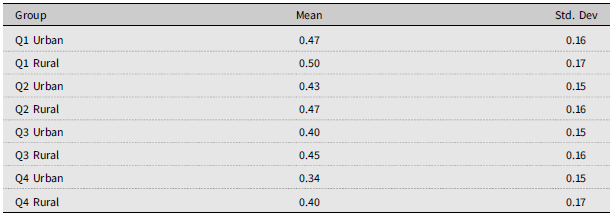
These patterns illustrate that food budget allocation not only varies by income but also within income quartiles and between urban and rural households. For reference, the mean and standard deviation of food budget shares for each subgroup are provided in Appendix Table A1. This granular approach captures nuances in household consumption behavior that are often obscured in aggregated analyses.

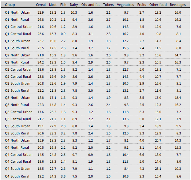
Shifting from general patterns under Engel’s Law, we now examine how Mexican households allocate their food budgets across specific food groups at home. Table 1 highlights differences by income, location, and region. In Q1, the lowest income group, cereals dominate expenditure in both urban and rural households, though the magnitude varies: rural households in the north and central regions allocate about 26% of their budget to cereals, compared to 22–23% in urban areas. This share declines steadily with income, reaching around 16% in north urban households and 19–20% in rural households by Q4. In contrast, meat expenditure rises consistently with income, particularly in central and southern regions, where urban Q4 households devote nearly one quarter of their food budget to meat.

Table 1. Food budget shares by income, region, and locality

Source: Own elaboration based on ENIGH data.

Regional and locality differences further illustrate heterogeneity in consumption. Rural households generally spend more on cereals, tubers, and oils, whereas urban households allocate higher shares to beverages and other foods, especially at higher income levels. For example, southern urban Q4 households spend more than 10% of their budget on beverages, and an additional 23% on other foods, reflecting a pronounced nutrition transition in urban areas. Fruits and vegetables play a larger role in central rural diets, with even low-income households allocating 16–18% of their budgets to fruits and vegetables, compared to 8–12% in other regions. Fish consumption, while low overall, is notably higher in southern households, reaching over 3% in rural Q4 households.

These patterns suggest that aggregating food budget shares by income or locality alone can obscure important regional dietary differences influenced by geography, culture, and food availability. Furthermore, the uneven allocation across food groups, and dominance of staples like cereals and meat versus smaller shares for other foods provides the basis for our entropy analysis, which captures both between-group and within-group dietary diversity across households.

Table 2 presents the entropy measures of dietary diversity in Mexico, capturing how evenly households allocate food expenditure across categories. Higher total entropy reflects greater dietary diversity, while decomposition into between-group (cereal + meat versus non-cereal + fish) and within-group (diversity within non-cereal + fish) entropy reveals the structure of food choices. To aid interpretation, between-group entropy is expressed as a percentage of total entropy.

Table 2. Entropy of the food consumption basket in Mexico

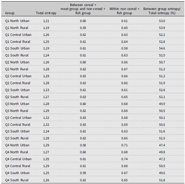
Source: Own elaboration based on ENIGH data.

Overall, dietary diversity tends to increase with income, particularly in urban areas, consistent with the Engel curve for variety. For example, Q4 Central Urban households reach a total entropy of 1.35, compared to 1.21 in Q1 North Urban, reflecting greater food variety with rising income. However, persistently lower diversity in rural Q4 households – such as Q4 South Rural (1.26) – indicates that income alone does not fully explain dietary outcomes.

Decomposition results show that between-group entropy declines with income, while within-group entropy rises, suggesting that wealthier households diversify more in non-staple categories, rather than shifting between broad food groups. The share of between-group entropy relative to total entropy falls from over 53% in Q1 to below 47% in Q4 urban households, highlighting this shift.

Regional variation adds further nuance. Central Mexico consistently exhibits the highest total entropy across all quartiles, particularly in urban areas, reflecting better access to diverse foods such as fruits, vegetables, and animal-source products (Pineda et al., 2023). In contrast, southern households show lower total and within-group entropy, even at higher income levels, indicating continued reliance on staple foods. These patterns suggest that structural and supply-side constraints, such as limited market access, poor infrastructure, and geographic isolation, may inhibit dietary diversification regardless of income. Evidence from southern states like Chiapas supports this interpretation, where persistent poverty and weak food environments contribute to food insecurity and childhood anemia (Cruz-Sánchez et al., 2024).

The urban–rural gap remains evident in most regions, reinforcing findings that rural populations face systemic barriers to accessing diverse diets (Mayen et al., 2014; Miller et al., 2022). Overall, while income is a key driver of dietary diversity, these results underscore the importance of regional context and structural inequalities in shaping food consumption patterns in Mexico.

Table 3 summarizes the demographic and socio-economic characteristics of households across four income quartiles (Q1 to Q4). Average household income rises significantly from Q1 (29,149 pesos) to Q4 (102,962 pesos), establishing a basis for examining the relationship between income and dietary diversity. The mean age of the household head increases from 48 years in Q1 to 53 years in Q4, suggesting a slight correlation between age and wealth. Average household size decreases with income, from four members in Q1 and Q2 to three in Q3 and Q4. The percentage of female-headed households also rises slightly from 29% in Q1 to 34% in Q4, indicating limited variation in gender dynamics across income levels.

Table 3. Household demographic and socioeconomic characteristics by income quartile

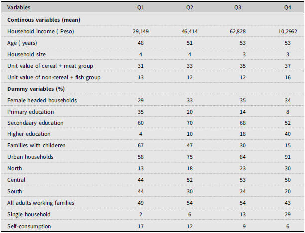
Source: Own elaboration based on ENIGH data.

Educational attainment shows a pronounced gradient: 35% of Q1 households have only primary education, while 40% of Q4 households have higher education, highlighting the strong link between education and income. The presence of children reduces markedly with income, from 67% in Q1 to 15% in Q4, suggesting that wealthier households may delay childbirth or prefer smaller families, which in turn influences food purchasing patterns. Urban residence also increases with income, from 58% in Q1 to 91% in Q4, reflecting greater market access for higher-income households. The share of households with all adults working remains relatively stable across quartiles (49–54%) but declines to 43% in Q4, while single households increase sharply from 2% in Q1 to 29% in Q4, indicating that wealthier individuals are more likely to live alone, potentially affecting dietary diversity and spending habits.

Unit values, defined as expenditure per unit of quantity, reveal important differences in food pricing across income levels. For the cereal + meat group, unit values rise steadily from 31 pesos in Q1 to 37 pesos in Q4, suggesting that higher-income households purchase more expensive or higher-quality staples and animal-source foods, potentially reflecting brand preferences, quality upgrades, or access to premium markets. For the non-cereal + fish group, unit values decline slightly from 13 pesos in Q1 to 12 pesos in Q2/Q3, before rising to 16 pesos in Q4, indicating that wealthier households increasingly diversify into more costly food categories such as fruits, vegetables, and processed items. The widening gap between staple and non-staple unit values underscores the role of purchasing power in shaping dietary diversity.

Regional composition also shifts across income levels. In Q1, households are evenly split between central and south (44% each), with only 13% from the north. By Q4, northern households comprise 30%, southern households 20%, and Central Mexico remains dominant throughout. These shifts highlight geographic disparities in income and access to diverse food markets. Finally, reliance on self-consumption declines with income, from 17% in Q1 to just 6% in Q4, suggesting that lower-income households depend more on subsistence strategies, while higher-income households purchase most of their food from markets.

5. Empirical results

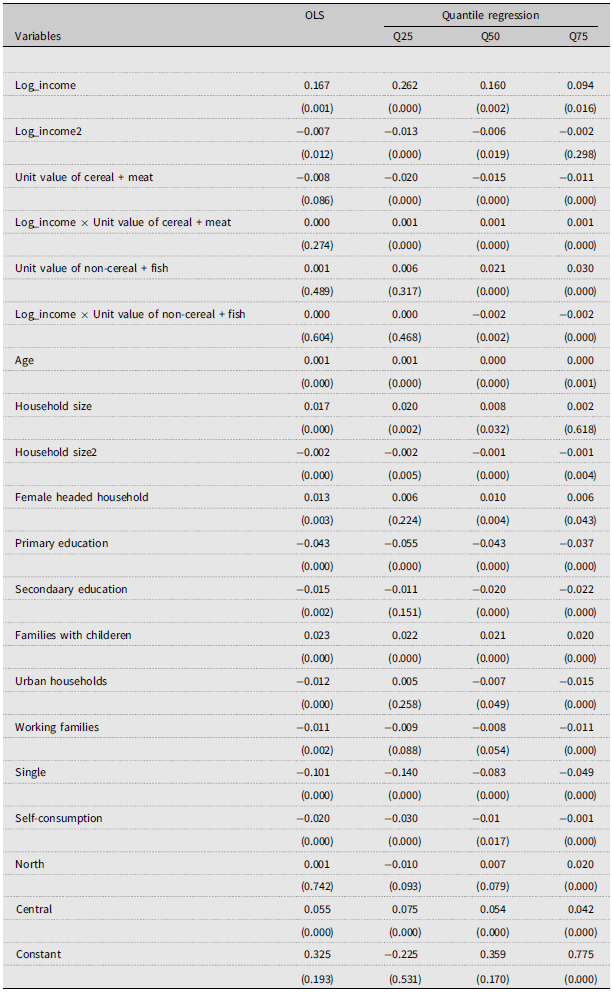
Table 4 presents the results of both OLS and quantile regressions examining how household characteristics, income, food prices, and location influence dietary diversity in Mexico. The results are broadly consistent across estimation methods, although the quantile regressions reveal important heterogeneities across the distribution of dietary diversity.

Table 4. OLS and quantile regression estimates of dietary diversity determinants

Note: p values are in parentheses.

Contrasting the OLS and quantile regression results highlight distributional differences that are masked in mean-based analysis (i.e., OLS-based). While OLS provides the average marginal effect across all households, quantile regression reveals that the impact of income, prices, and household characteristics varies along the dietary diversity distribution. Measured as the logarithm of total household income, income is positively associated with dietary diversity, in line with Engel’s Law for variety (Chai et al., 2015; Clements and Si, 2018), with the strongest effects at lower quantiles. The negative coefficient on the squared income term indicates diminishing marginal effects, with wealthier households already accessing a wide range of food groups, so additional income has a smaller impact.

Household composition exhibits a complex relationship with dietary diversity. Larger households are associated with lower diversity at lower quantiles, likely reflecting budget constraints and the prioritization of staple foods, but the positive squared term suggests that very large households may achieve greater variety through economies of scale (Jayasinghe and Smith, 2021; Lanjouw and Ravallion, 1995) or differing preferences among members. Families with children tend to have more diverse diets, particularly in lower- and middle-income households, reflecting the need to provide nutritionally varied meals. In contrast, single households consistently show lower diversity across all quantiles, while female-headed households display mixed effects, with lower diversity at the lower quantiles but higher diversity at the upper quantiles, suggesting that the benefits of female decision-making emerge more clearly when resources are sufficient. Consistent with the literature, we find that older household heads are slightly more likely to have greater dietary diversity, reflecting more experience in household food management, while younger heads may experiment with a broader range of foods (Korir et al., 2023; Thiele et al., 2017).

Education also plays an important role, with households headed by individuals with lower levels of education exhibiting significantly lower dietary diversity, particularly at higher quantiles, highlighting the influence of knowledge on informed food choices (Olabisi et al., 2021; Thiele and Weiss, 2003). The results also indicate that self-consumption is negatively associated with dietary diversity, especially among households with lower diversity. Relying on home-produced foods may limit access to diverse food groups compared to market purchases, consistent with evidence that self-production can increase dependence on staples (Muthini et al., 2020; Sibhatu and Qaim, 2018). While it supports food security, self-consumption may not improve dietary diversity.

Time constraints appear to affect dietary patterns as well. Households in which all adult members are engaged in income-generating activities show consistently negative effects, indicating that limited time for meal planning and preparation can reduce dietary diversity. This finding aligns with evidence from other studies showing that dual-earner households often rely on more repetitive or convenient diets (Komatsu et al., 2018; Koomson et al., 2025). The role of food prices is also evident in the results. Higher unit values of cereals and meat are associated with slightly lower dietary diversity, consistent with the idea that rising staple costs crowd out spending on other food groups. However, the interaction between income and staple prices is positive, suggesting that wealthier households are less constrained by staple price increases. Similarly, higher prices for non-cereal + fish items reduce diversity among poorer households, whereas wealthier households can maintain variety despite higher costs, illustrating the critical role of affordability in shaping diet quality (Batis et al., 2020; Huffman et al., 2023).

Spatial differences further shape dietary diversity outcomes. Urban households tend to exhibit higher diversity at the upper quantiles, reflecting broader food environments and better access to diverse markets (De Filippo et al., 2021; Van Bui et al., 2016). Yet at lower quantiles, urban residence is negatively associated with diversity, possibly due to higher food prices and a reliance on convenience foods among poorer urban households. Regional disparities are also evident, with households in the south consistently displaying lower diversity compared to those in the central region. In the north, diversity is only slightly higher among households at the upper end of the distribution, highlighting the role of structural and geographic factors in shaping dietary patterns (Pineda et al., 2023).

Overall, these results suggest that dietary diversity in Mexico is determined by a combination of income, household composition, education, affordability, and geography. While income growth clearly supports diversification, other structural and contextual factors influence how different households translate available resources into varied diets. The findings underscore the need for policies that address affordability, knowledge, and access to diverse foods in order to improve dietary outcomes across socio-economic and regional groups.

6. Conclusions and policy implications

This study provides comprehensive evidence on the socioeconomic, demographic, and geographic determinants of food consumption patterns and dietary diversity in Mexico. Consistent with Engel’s Law, the share of food in total household expenditure declines with income, but considerable heterogeneity exists within income quartiles and across urban and rural contexts. Poorer rural households, particularly in South Mexico, remain heavily reliant on cereals and meat, while higher-income urban households in Central Mexico exhibit greater dietary diversity, allocating more spending to fruits, vegetables, beverages, and other non-staple foods. These patterns demonstrate that aggregating dietary behaviors by income or locality alone risks masking substantial heterogeneity shaped by geography, food environments, and cultural preferences.

Entropy-based measures confirm that income growth promotes dietary diversification, but with diminishing marginal effects at higher income levels. The strongest benefits occur in lower-income households, suggesting that targeted interventions for resource-poor households could yield substantial improvements in dietary quality. Household characteristics such as size and composition influence diversity in non-linear ways: larger households face budget constraints that may reduce variety, but beyond a threshold economies of scale can enhance diversity. Education is also a key determinant, with households headed by less-educated individuals consistently reporting lower dietary diversity, highlighting the role of knowledge and awareness alongside financial capacity.

Food prices are a critical constraint, particularly for lower-income households. Higher unit values for staples and non-staples reduce diversity, while wealthier households can better absorb higher costs and maintain a varied diet. Regional disparities further compound these effects: households in Central Mexico benefit from stronger market integration and access to diverse foods, whereas southern households remain disadvantaged despite income growth, reflecting structural barriers to dietary diversification. Urban households generally enjoy higher diversity due to broader market access, but the poorest urban households may still face constraints, highlighting the complex interplay of income, location, and food environment.

From a policy perspective, these results illustrate the need for income-sensitive, regionally tailored interventions. For low-income households, particularly in rural and southern regions, programs such as targeted subsidies, vouchers for nutrient-dense foods, or the expansion of the Canasta Básica Segalmex-Diconsa to include more diverse and nutrient-rich items could improve dietary quality. Strengthening rural food markets and addressing structural bottlenecks in supply chains would further support diversification. Education programs targeting households with lower levels of schooling could reinforce the adoption of diverse and nutritious diets, even when they face resource constraints. Importantly, our quantile regression results show that policy impacts may differ across households. Interventions targeting the poorest or those with the least diverse diets are likely to yield greater improvements than measures aimed at households already enjoying diverse diets. This highlights the value of distribution-sensitive approaches that complement average-effect analyses, suggesting that policies such as targeted subsidies, nutrition education, or region-specific programs should be tailored to the characteristics and needs of different household groups.

Some limitations of the Entropy Index should be noted. Unlike simple counts of food groups, entropy scores can be less intuitive for policymakers. They are also sensitive to how foods are grouped: our two-group partition (cereal + meat versus non-cereal + fish) captures broad patterns, but different groupings could alter absolute values. Despite this, the index flexibly reflects both the number of foods consumed and how expenditure is distributed, providing useful insights for designing interventions that address affordability and access. Methodologically, this study demonstrates the value of combining entropy-based measures with quantile regression, capturing heterogeneities often overlooked by mean-based approaches. Future research could extend this analysis to food consumed away from home and intra-household allocation, and explore causal pathways using longitudinal or experimental data.