


Introduction
Recently, researchers have started to define political polarization based on people's feelings towards parties and their supporters, instead of the classic ideological divergence approach. A tendency among party supporters to view other parties and their supporters as disliked out‐groups, while holding positive in‐party feelings, has been labelled as affective polarization (Iyengar et al., Reference Iyengar, Sood and Lelkes2012; Lelkes, Reference Lelkes2016). Affective polarization has been shown to be a problematic phenomenon with dangerous consequences. It can lead to policy gridlock at the elite level and decrease trust towards institutions and satisfaction with democracy among voters (Hetherington & Rudolph, Reference Hetherington and Rudolph2015; Oscarsson & Holmberg, Reference Oscarsson and Holmberg2020). Moreover, intense partisan feelings tend to go further than the political sphere and divide the whole society into antagonistic groups who perceive each other as enemies and might even condone political violence against the out‐group (Martherus et al., Reference Martherus, Martinez, Piff and Theodoridis2021; McCoy et al., Reference McCoy, Rahman and Somer2018). Events such as the storming of the Capitol on 6 January 2021 vividly illustrate the dangers of such political resentment.
Affective polarization research has hitherto focused mostly on the United States context, where the level of partisan animosity has soared over the past decades (Iyengar et al., Reference Iyengar, Lelkes, Levendusky, Malhotra and Westwood2019). In recent years, research on the topic has also proliferated in other parts of the world, predominantly in Europe. A rapidly increasing volume of literature has by now established that affective polarization is undoubtedly present also in European (multi)party systems, although the levels of it vary majorly across countries, as different countries exhibit diverging dynamics (see Boxell et al., Reference Boxell, Gentzkow and Shapiro2020; Gidron et al., Reference Gidron, Adams and Horne2020; Lauka et al., Reference Lauka, McCoy and Firat2018; Reiljan, Reference Reiljan2020; Reiljan & Ryan, Reference Reiljan and Ryan2021; Wagner, Reference Wagner2021; Ward & Tavits, Reference Ward and Tavits2019; Westwood et al., Reference Westwood, Iyengar, Walgrave, Leonisio, Miller and Strijbis2018).
Currently, the cross‐national research on affective polarization has focused on variations across countries, over time or between individuals. Thereby, it implicitly assumes a homogeneous regional distribution of affective polarization within countries. Consequently, when studying the potential foundations of affective polarization, the attention has gone to country‐ or individual‐level predictors (Boxell et al., Reference Boxell, Gentzkow and Shapiro2020; Gidron et al., Reference Gidron, Adams and Horne2020; Harteveld, Reference Harteveld2021), ignoring regional characteristics that might drive partisan feelings. In the U.S. literature on affective polarization, the regional aspect has also been mostly overlooked, although some pieces of evidence suggest notable geographical divergences. For example, Iyengar et al. (Reference Iyengar, Sood and Lelkes2012) found that residents of the so‐called battleground states exhibit higher levels of affective polarization, and a study by Tobias Konitzer (reported in The Atlantic Footnote 1) indicated that the level of partisan prejudice could vary significantly across counties in the United States. Yet, we lack a systematic comparative study of regional variations in affective polarization either in the United States or in Europe.
This gap is surprising, as many recent studies investigating Brexit or the rise of populist radical right parties show that political attitudes and radical voting patterns vary heavily across regions (Ford & Jennings, Reference Ford and Jennings2020; Gimpel et al., Reference Gimpel, Lovin, Moy and Reeves2020; Stockemer, Reference Stockemer2017). Authors have emphasized how long‐term structural socio‐economic changes have contributed to increasing geographical disparities within countries, with some (often urban) regions attracting economic development, skilled workforce and capital, and other (rural) areas facing decline (McKay, Reference McKay2019). The development of these ‘left behind’ areas and ‘places that don't matter’ (Rodriguez‐Pose, Reference Rodriguez‐Pose2018) has been pinpointed as drivers of a ‘geography of discontent’ (McCann, Reference McCann2020). Such regional socio‐economic disparities contribute to widening the gap in political attitudes (Cramer, Reference Cramer2016) and have been linked to the development of radical, anti‐system, populist voting behaviours (Becker et al., Reference Becker, Fetzer and Novy2017; bin Zaid & Joshi, Reference Bin Zaid and Joshi2018; Greve et al., Reference Greve, Fritsch and Wyrwich2021; McKay, Reference McKay2019; Rodden, Reference Rodden2019; Van Hauwaert et al., Reference Van Hauwaert, Schimpf and Dandoy2019). However, this recent revival of the regional approach has mainly focused on Britain and the United States and has not been connected to the literature on affective polarization.
This research note aims at filling this gap by investigating the scope of regional variations in levels of affective polarization across Europe. After a brief conceptual and methodological discussion, we present disaggregated data on affective polarization in 190 regions in 30 countries, over a period ranging from 1996 to 2019. Subsequently, we map affective polarization scores across these regions, both cross‐sectionally and longitudinally. Our results reveal that regional variations are highly significant in the European context and underline the potential relevance of a regional approach in the study of affective polarization.
Defining and measuring affective polarization at a regional level
Our main goal is to measure affective polarization at the regional level and to contrast it to national scores to highlight the interest in a disaggregated approach. Affective polarization is usually measured at the individual level by survey items asking respondents to rate their feelings towards parties/party supporters (Iyengar et al., Reference Iyengar, Lelkes, Levendusky, Malhotra and Westwood2019). In the U.S. two‐party context where most of the affective polarization research has hitherto been conducted, the degree of affective polarization is determined by the difference in the evaluations towards the two main parties. Applying this concept to multiparty systems, however, implies some conceptual and methodological elaborations.
In a multiparty context, voters can simultaneously like (or dislike) more than just one party, which makes it significantly more complicated to grasp the degree of affective polarization. Some authors have defined affective polarization as the difference between feelings towards one in‐party and several out‐parties (Gidron et al., Reference Gidron, Adams and Horne2020; Reiljan, Reference Reiljan2020). By clearly defining a partisan in‐group, this definition aligns more closely with the “partisanship as a social identity” approach as it was originally proposed by Iyengar et al. (Reference Iyengar, Sood and Lelkes2012). An alternative approach suggests dropping the in‐ and out‐party distinction and conceptualizes affective polarization as the extent to which the partisan landscape is divided into distinct (affective) camps/blocs that may consist of one or more parties (Kekkonen & Ylä‐Anttila, Reference Kekkonen and Ylä‐Anttila2021; Wagner, Reference Wagner2021). By focusing on the overall distribution of positive and negative feelings towards parties, this definition could better account for the potential reality of voters sympathizing with more than one party.
These two definitions of affective polarization in multiparty systems translate into two alternative measurement approaches. In line with the first definition, Reiljan (Reference Reiljan2020) proposes the Affective Polarization Index that calculates the average like–dislike difference between the one party that the voter feels closest to (in‐party) and all relevant out‐parties (see also Boxell et al., Reference Boxell, Gentzkow and Shapiro2020; Gidron et al., Reference Gidron, Adams and Horne2020). To operationalize the second definition, Wagner (Reference Wagner2021) lays out the Spread‐of‐Scores index that measures the spread of party like‐dislike evaluations around the respondent's mean score (see also Ward & Tavits, Reference Ward and Tavits2019, for a similar approach). Both authors also agree that in a multiparty context, the size of the parties should be taken into account. Thus, they weight the measures with party vote shares, so that larger parties have a higher impact on the index values (Dalton, Reference Dalton2008; Reiljan, Reference Reiljan2020; Wagner, Reference Wagner2021).
The theoretical and empirical debate on how to best capture affective polarization in multiparty systems is still far from resolved. However, both approaches described above have been accepted by researchers and are likely to give a reasonably accurate estimate of the degree of affective polarization in multiparty contexts. The most suitable measurement depends on the research problem and available data.
In this paper, we rely on Wagner's definition and his matching spread/standard deviation measure for theoretical and empirical reasons. There are likely to be substantial regional variations in party structure: the popularity of different parties varies and sometimes even the parties that are running for office are not identical across regions. In such a case, a measure of general dispersion of feelings towards parties should ensure better comparability than an approach that groups voters based on their party preference. From the empirical perspective, dividing respondents into partisan groups based on their party preference is problematic in the case where there are few respondents (and even fewer of them having a partisan identification) per regional unit. As in our data the number of respondents is rather small in some regions, Wagner's spread approach is more easily applicable.
Data and measurements
We first retrieve individual‐level data from the Comparative Study of Electoral Systems (CSES) dataset,Footnote 2 where a question asking respondents to evaluate each party in the national ballot box on a 0–10 scale is available in all waves.Footnote 3 We then aggregate measures of affective polarization at the regional and national levels.
As explained, we use the weighted version of Wagner's Spread‐of‐Scores index of affective polarization (Wagner, Reference Wagner2021).
The index is first computed at the individual level based on the following equation:
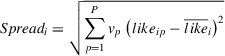 $\begin{equation*}{\rm{\;}}Sprea{d_i} = \sqrt {\mathop \sum \limits_{p = 1}^P {v_p}\;{{\left( {lik{e_{ip}} - {{\overline {like} }_i}} \right)}^2}} \;\end{equation*}$
where subscripts i and p indicate each survey respondent and each party in the national ballot box, Vp represents the party vote share, like signifies the like–dislike evaluation of individual i towards a party p on a scale from 0 (strong dislike) to 10, and
 $\overline {like} $ is the respondent's i’s average party like–dislike score. After this computation, we end up with an affective polarization score for a total of 143,857 individuals.
Thereafter, we aggregate these individual‐level scores at the regional and country levels. We group survey respondents by their country and region of residence and calculate the average level of affective polarization for each country and region.Footnote 4 We restrict the analysis to countries with the Nomenclature of territorial units for statistics (NUTS) classification system provided by the European Commission,Footnote 5 to have a homogeneous method of spatial aggregation across countries. In the Appendix, we provide more details about the way we assign a NUTS classification to each region in the CSES dataset.Footnote 6 CSES covers a time span of over 20 years (1996–2019), and most countries are included with more than one election. Consequently, there are three levels of data in our dataset: regions and elections, both nested within countries. Our final dataset includes affective polarization scores for 30 countries, 190 regions, and 105 elections.
We contrast country and regional affective polarization scores both cross‐sectionally and longitudinally. Our cross‐sectional analysis presents the aggregated data at the country/regional level by computing the mean country/regional affective polarization score, pooled across all available elections. We also provide a longitudinal analysis that offers a dynamic interpretation of country/regional levels of affective polarization by dividing the time span at disposal (i.e., 1996–2019) into two sub‐periods, with the Great Recession (2008) as the exogenous shock separating the two.
As mentioned before, a low number of observations per region is a problem that we faced with the data at our disposal. In ca. 6 per cent of the cases, the number of respondents per region remains under 30. Also, in some smaller European countries, the number of regions is low (one to two regions per country). In our analyses below, the maps include all regions, regardless of the N of respondents and the N of regions per country. However, in the analysis where we compare the cross‐regional and cross‐national variation in the levels of affective polarization, we have taken a more cautious approach and excluded regions with less than 30 respondents and countries with less than three regions.
Cross‐sectional analysis of affective polarization
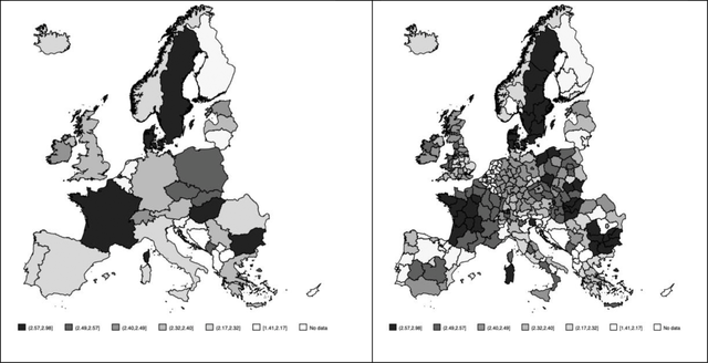
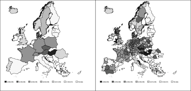
Our cross‐sectional analysis contrasts affective polarization scores aggregated at the country level and at the region level, pooled for the entire period (see maps in Figure 1).Footnote 7

Figure 1. Affective polarization index by country vs. by region
Country‐level scores oppose countries with high levels of affective polarization (e.g., Bulgaria, France and Hungary) and moderately high levels (e.g., Czech Republic, Poland and Slovakia), to countries with moderately low (e.g., Norway, Romania and Spain) or low levels (e.g., Belgium, Finland, the Netherlands and Slovenia).
However, when disaggregating at the regional level, the picture is much more nuanced. Some countries present very heterogeneous scores at the regional level. For instance, France is split in half, with western regions displaying higher levels than eastern regions. Poland and Hungary offer an internally heterogeneous picture as well. Similarly, some countries in (light) blue in the country map display heterogeneous regional patterns. Italy's regional map reveals pockets of regions with higher levels of affective polarization (e.g., Sardinia). The same pattern can be observed in Romania and Spain, the latter being the country that displays the highest within‐country variation in our sample. Belgium and Portugal are split in half, with southern regions displaying lower levels of affective polarization. Countries with scores close to the central intervals are also internally heterogeneous. The United Kingdom has split across a north–south and west–east divide; Germany, Greece and Switzerland also show some notable regional variations. These maps, shown side‐by‐side, help visualize how aggregating scores at the country level masks within‐country variations, and how high or low scores in countries can be driven by some regions only.
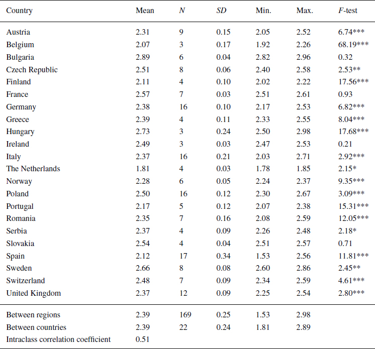
To go beyond visual contrasts, Table 1 displays the summary statistics for our cross‐sectional analysis, limiting the sample to countries with at least three regions and regions with at least 30 observations. For each country, we specify the average affective polarization score at the country level (mean), and we indicate the number of regions included, the standard deviation around the mean for these regions, and the minimum and maximum regional scores. It allows us to contrast within‐country variations and between‐country differences in affective polarization scores.
Table 1. Cross‐sectional affective polarization scores by country and regions (entire period)

At the country level, we can see that the Netherlands displays the lowest average score (1.81) and Bulgaria the highest (2.89). When disaggregating by region, we see that the lowest score (1.53) is in Spain and the highest (2.98) in Hungary. Overall, the range of scores is, therefore, larger across regions.
The last column in Table 1 displays the analysis of variance (ANOVA) F‐test to statistically assess the equality of means across regions, within countries. Only in four countries (Bulgaria, Ireland, France and Slovakia), we cannot reject the null hypothesis of equal means across regions. Table 1 also reports the intraclass correlation coefficient (ICC), a measure commonly used in the literature to show how much of the total variation in a dependent variable can be explained by between‐ and within‐clusters differences (Bernauer & Vatter, Reference Bernauer and Vatter2012; Curini, Reference Curini2018). In our analysis, the coefficient refers to the between‐ and within‐countries dynamics. The ICC ranges from 0 to 1, with 1 indicating perfect within‐country homogeneity. The reported coefficient (0.51) signals that approximately half of the variation in affective polarization scores is due to within‐countries dynamics, thus further justifying our claims.
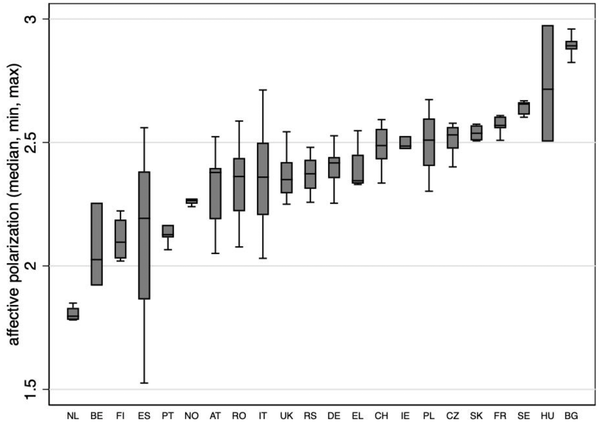
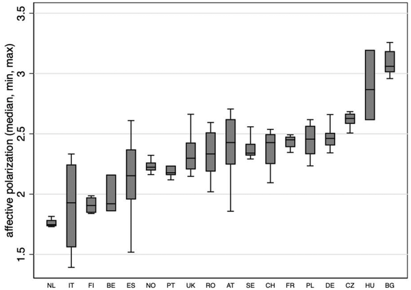
The information contained in Table 1 is plotted in Figure 2. For each country, we report the national median and the within‐country range of affective polarization scores. Figure 2 illustrates three interesting trends. First, data show that within‐country variation is at least as relevant as cross‐country differences. For instance, the gap between Navarre and Castile‐La Mancha in Spain (respectively, showing an affective polarization score of 1.53 and 2.56) is as large as the gap between the first and last country in the national ranking of affective polarization scores (i.e., the Netherlands and Bulgaria). Second, the degree of within‐country variation is very heterogeneous across countries, with countries showing huge internal differences (e.g., Spain, Italy and Hungary) that contrast with very homogeneous national contexts (e.g., the Netherlands, Norway, and Bulgaria). Third, there is not a clear‐cut correlation between the degree of within‐country heterogeneity and the median country‐level of affective polarization. Countries with high within‐country heterogeneity are present at both extremes of the distribution of the affective polarization score (e.g., Belgium and Hungary).

Figure 2. Affective polarization scores by country (median, minimum, maximum), the entire period
Longitudinal analysis of affective polarization
Our longitudinal analysis contrasts affective polarization scores aggregated at the country and the region level, before and after 2008.
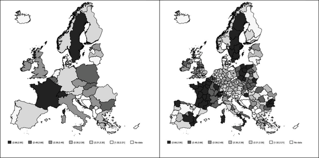
Figure 3 (scores pre‐2008) and Figure 4 (scores post‐2008) demonstrate how affective polarization levels have increased in most countries between the two periods, except Austria, Bulgaria, Czech Republic, Germany, Hungary, Iceland and Portugal.Footnote 8

Figure 3. Affective polarization by country versus by region, pre‐2008

Figure 4. Affective polarization by country versus by region, post‐2008
As with our cross‐sectional analysis, disaggregating affective polarization scores at the regional level provides a more nuanced picture. It highlights contrasting situations. Italy, Poland, Romania, Spain or the United Kingdom are striking examples of countries characterized by regions with high and low levels of affective polarization that co‐exist. This diversity of within‐country situations is even more marked in the post‐2008 period. The figures also show that the national increase in affective polarization is sometimes driven by sharp increases in some specific regions. In Spain, Galicia, Valencia and Murcia display a sharp increase that pushes the national average up, even if affective polarization scores remain stable in other regions (Aragon, Castilla y Leon). This suggests that it is not so much something happening in Spain in general that can account for the change over time. Rather, it is only by looking at what is happening at a more disaggregated level that we could shed light on this long‐term trend.
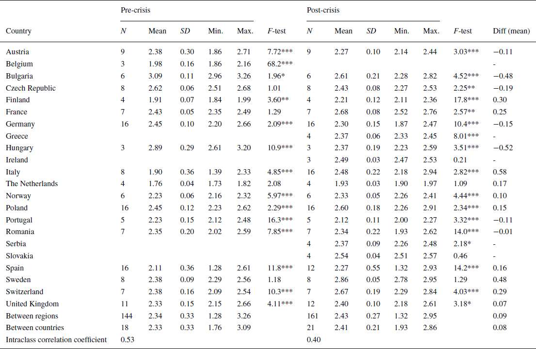
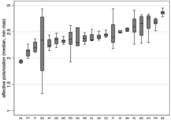
Table 2 displays the same summary statistics as for our cross‐sectional analysis, but for the two sub‐periods (pre‐ and post‐2008), again limited to countries with at least three regions and regions with at least 30 observations. At the country level pre‐2008, the Netherlands displays the lowest average score (1.76) and Bulgaria the highest (3.09). When disaggregating by region, we see that the lowest score (1.28) is in Spain and the highest (3.26) in Bulgaria. The spread of scores is again larger across regions. A similar pattern can be observed after 2008. The country with the lowest score is still the Netherlands (1.93) and the one with the highest score is Sweden (2.86). When looking at regional variations, the lowest score (1.32) is again in Spain and the highest (2.95) in Sweden. Overall, we show that affective polarization has, on average, increased over time, with Italy and Sweden showing the largest increase.Footnote 9
Table 2. Longitudinal affective polarization scores by country and regions (pre‐ and post‐crisis)

Table 2 also reports the ANOVA F‐test and ICC coefficients for the two periods. The latter indicates that the relevance of the within‐country heterogeneity has increased over time, accounting for the 60 per cent of the total variation in the affective polarization scores in the post‐2008 period.
The information contained in Table 2 is plotted in Figures 5 and 6. For each period and country, we plot the national median and the within‐country range of affective polarization scores. It confirms that within‐country variation is at least as relevant as cross‐country differences. It also confirms the heterogeneity of national situations, with some countries displaying very high levels of within‐country variation and others being more homogeneous.

Figure 5. Affective polarization scores by country (median, minimum, maximum), pre‐2008

Figure 6. Affective polarization scores by country (median, minimum, maximum), post‐2008
Conclusion
This research note investigated the scope of regional variation in levels of affective polarization across Europe and contrasted it with national variations to highlight the interest in a disaggregated approach. Overall, our cross‐sectional and longitudinal analyses have first stressed that more than half of the variation in affective polarization scores can be attributed to within‐country heterogeneity. Second, we demonstrated that while some countries display rather homogeneous regional patterns, others exhibit heterogeneous scores. Third, we showed how the increase in the affective polarization scores over time at the national level can be driven by sharp changes in some regions only, while other regions remain stable. It highlights how national averages can be driven up or down by some regions. In some instances, looking at national factors will not be enough to account for a change over time. It is only by looking at what is happening at a more disaggregated level that we could shed light on this long‐term trend.
These findings point to the added value of a regional approach to the study of affective polarization and its drivers. Existing analyses have often put the emphasis on macro‐level drivers of affective polarization, such as institutional and structural factors (Westwood et al., Reference Westwood, Iyengar, Walgrave, Leonisio, Miller and Strijbis2018; Gidron et al., Reference Gidron, Adams and Horne2020); however, high variations within countries indicate that macro‐level factors may be less relevant than assumed. Similarly, contrasting findings regarding the effects of economic inequalities or economic downturns on levels of affective polarization (Boxell et al., Reference Boxell, Gentzkow and Shapiro2020; Gidron et al., Reference Gidron, Adams and Horne2020) may be due to a problem of level of analysis. What matters may not be national socio‐economic performances, but rather socio‐economic disparities across regions, as well as long‐term structural regional decline. From a methodological perspective, a regional approach increases the number of observations. Instead of comparing affective polarization across a few dozens of European countries, we can evaluate it across hundreds of regions and produce better models.
Our results pave the way for at least three avenues for future research: investigating the drivers of regional variation in levels of affective polarization, understanding why countries present more or less heterogeneous patterns, and analysing how regional factors can help us better understand the change in affective polarization over time.
Funding Information
Bettarelli received funding from the European Union's Horizon 2020 research and innovation programme under the Marie Sklodowska‐Curie grant agreement no. 801505. Reiljan received funding from the Estonian Research Council mobility grant no. MOBJD607. Van Haute received funding from the FWO‐FNRS EoS grant no. 30431006.
Conflict of interest
The authors declare that they have no competing interests.
Data availability statement
Data and replication files are available online as Supporting Information. All analyses are run based on publicly available datasets listed in Appendix.
Appendix
List of countries, regions and elections included in the dataset

Note: The regional classification method in the CSES dataset is not homogeneous across countries. Column 3 (CSES regions) reports the regional classification available in the CSES dataset, where OTHER indicates criteria that do not perfectly match with NUTS classification. In cases of OTHER, we have matched regions with the closest NUTS classification. Column 4 (Paper regions) defines the spatial aggregation used in this analysis for each country. Note that we do not consider overseas territories. We have excluded Turkey from our analysis. In fact, previous research has identified that Turkey is a country with extremely high levels of affective polarization (Lauka et al., Reference Lauka, McCoy and Firat2018; Wagner, Reference Wagner2021), making it an outlier case. For the longitudinal analysis, we used 2008 as the year separating two sub‐periods. Two countries in our sample had elections in 2008, Austria and Spain. In order to have both countries in both sub‐periods, we have classified Austria's 2008 elections as pre‐2008, while Spain's 2008 elections as post‐2008.
Online Appendix
Additional supporting information may be found in the Online Appendix section at the end of the article:
Supplementary material


 Open access