The third Konus-Wind catalogue of short gamma-ray bursts

Abstract

In this catalogue, we present the results of a systematic study of 199 short gamma-ray bursts (GRBs) detected by Konus-Wind between 1 January 2011 and 31 August 2021. The catalogue extends the Second Catalogue of short GRBs covering the period 1994–2010 by ten years of data. The resulting Konus-Wind short GRB sample includes 494 bursts. From temporal and spectral analyses of the sample, we provide the burst durations, spectral lags, estimates of the minimum variability timescales, rise and decay times, the results of spectral fits with three model functions, the total energy fluences, and the peak energy fluxes of the bursts. We present statistical distributions of these parameters for the complete set of 494 short GRBs detected in 1994–2021. We discuss in detail the properties of the bursts with extended emission in the context of the whole short GRB population. Finally, we consider the results in the context of the Type I (merger-origin)/Type II (collapsar-origin) classification and discuss the extragalactic magnetar giant flare subsample.

1. Introduction

Cosmological gamma-ray bursts (GRBs) are thought to be related to at least two distinct classes of catastrophic events: the merger of binary compact objects, such as two neutron stars or a neutron star and a black hole, and the core collapse of a massive star. The former may produce a short-duration GRB, with a duration less than $\sim 2$ s, the so-called Type I GRB, while the latter occasionally produce typically long-duration GRB, showing softer spectra and non-negligible spectral lag, Type II GRBs (see, e.g., Zhang, 2006; Zhang et al., 2009, for more information on the Type I/II classification scheme).

In fact, the duration distributions of Type I and Type II GRBs significantly overlap. The shortest Type II burst discovered so far – GRB 200826A (Ahumada et al., 2021) had a duration of $\lesssim 1$ s, while GRB 170817A, the counterpart of the gravitational-wave event GW 170817 and kilonova AT2017gfo from a binary neutron star merger (Abbott et al., 2017), had a duration of $\sim 2$ s. Moreover, for a number of nearby short/hard GRBs it was possible to obtain deep upper limits on both supernova and kilonova emission (see, e.g., Ferro et al., 2023), which illustrates the complexity of the physical classification of short GRBs. On the other hand, a number of long-duration GRBs showed afterglow features similar to kilonova emission produced by a binary merger, in particular two recent bursts: GRB 211211A (Rastinejad et al., 2022; Troja et al., 2022; Barnes & Metzger, 2023) and GRB230307A (Levan et al., 2023b,a; Dichiara et al., 2023). These bursts show a short initial episode followed by a bright, tens of seconds-long main phase, which may have a similar origin to the so-called extended emission (EE) observed in a fraction of short GRBs (sGRBs). The EE is a weaker emission component that follows the short initial pulse (IP) and has been observed in a fraction of sGRBs by various experiments: CGRO-BATSE (Burenin, 2000; Norris & Bonnell, 2006; Bostancı et al., 2013), Konus-Wind (KW; Mazets et al., 2002; Svinkin et al., 2016), INTEGRAL-SPI-ACS (Minaev et al., 2010), Swift-BAT (Norris et al., 2011; Sakamoto et al., 2011), Fermi-GBM (Kaneko et al., 2015), and AGILE-MCAL (Ursi et al., 2022).

In addition to cosmological GRBs, the observed sGRB population includes magnetar giant flares (MGFs) in nearby galaxies (Svinkin et al., 2021; Burns et al., 2021), which may be identified by localisation and distinct temporal and spectral evolution.

Thus, a detailed analysis of a large sample of sGRBs, including candidates for sGRBs with EE, may contribute significantly to the understanding of both the collapsar and the merger origin scenarios.

In this catalogue, we update the results presented in the Second sGRB Catalogue (Svinkin et al., 2016, hereafter S16) to include the analysis of 199 sGRBs detected by KW between 2011 January 1 and 2021 August 31 (494 sGRBs in total). The burst sample selection criteria and localisations are presented in Svinkin et al. (2019, 2022).

This catalogue is organised as follows. We start with a short description of the KW instrument details in Section 2. In Section 3, we provide details of the KW sGRB sample. We describe the light curve and spectral analysis procedures and present the results in Section 4. In Section 5, we discuss the results. In Section 6, we give a summary and our conclusions.

Throughout the paper, all errors are reported at the 68% confidence level (CL).

2. Konus-Wind

The KW (Aptekar et al., 1995) spectrometer was launched on board the NASA Wind spacecraft in November 1994 and has operated until the present day. The instrument consists of two identical NaI(Tl) detectors, S1 and S2, each with a 2 $\pi$ field of view and a nominal energy band of 10 keV-10 MeV. The detectors are mounted on opposite faces of the rotationally stabilised spacecraft, such that one detector (S1) points toward the south ecliptic pole, thereby observing the southern ecliptic hemisphere, while the other (S2) observes the northern ecliptic hemisphere.

KW operates in two modes: waiting and triggered. In the waiting mode, light curves in three wide energy bands with nominal boundaries G1 (13–50 keV), G2 (50–200 keV), and G3 (200–760 keV) are recorded with a time resolution of 2.944 s. The switching to the triggered mode occurs at a statistically significant count rate increase in the G2 band. In the triggered mode, light curves are recorded in the same bands G1, G2, and G3 from $-0.512$ s to 229.632 s relative to the trigger time with a varying time resolution. The time resolution is 2 ms for the interval between $-0.512$ s and 0.512 s, 16 ms for the 0.512–33.280 s, 64 ms for the 33.280–98.816 s relative to the trigger time, and 256 ms for the remaining triggered time history. In the triggered mode, 64 multichannel spectra are measured starting from the trigger time by two pulse-height analysers PHA1 (63 channels, nominal boundaries 13–760 keV) and PHA2 (60 channels, nominal boundaries 250 keV–10 MeV). The first four spectra are measured with a fixed accumulation time of 64 ms to study short bursts. For the subsequent 52 spectra, an adaptive system determines the accumulation times, which may vary from 0.256 s to 8.192 s depending on the current count rate in the G2 energy band (the higher count rates produce shorter accumulation times). The last 8 spectra have an accumulation time of 8.192 s each. As a result, the duration of spectral measurements varies from 79.104 s to 491.776 s.

The detector response matrix (DRM) was calculated using GEANT4 toolkit (Agostinelli et al., 2003; Allison et al., 2006; Allison et al., 2016). In this work, as compared to S16, we used an updated DRM that characterises the detector response more accurately. We further discuss the impact of the DRM update on the results.

The detector gain slowly decreases with time. As of 2021, the detector energy ranges have shifted from the nominal 13 keV–10 MeV to 28 keV–20 MeV (S1) and 22 keV–16 MeV (S2), and the light curve and the spectral measurement bands have shifted accordingly. A more detailed instrument description can be found in S16 and Lysenko et al. (2022).

3. The sGRB sample

Between the start of the operation on 1994 November 12 and 2021 August 31, KW triggered on 3397 GRBs. During the interval covered by this catalogue, KW detected 1365 GRBs. From the updated analysis (Svinkin et al., 2019) of KW burst durations $T_{50}$ and $T_{90}$ ^a , we adopted $T_{50} = 0.7$ s as the boundary between short and long KW GRBs, which yielded 198 ^b sGRBs detected between 2011 January and 2021 August.

Previous studies suggest that some of the sGRBs can, in fact, be initial pulses of magnetar giant flares (MGFs) from nearby galaxies (see, e.g., Svinkin et al., 2015; Burns et al., 2021). The sample of KW sGRBs detected up to August 2021 contains only four bursts whose localisation regions overlap nearby galaxies and which can thus be interpreted as extragalactic MGF candidates. These bursts are GRB 051103 in the M81/M82 group of galaxies (Frederiks et al., 2007), GRB 070201 in the Andromeda galaxy M31 (Mazets et al., 2008), GRB 070222 in the M83 galaxy (Burns et al., 2021), and GRB 200415A in the Sculptor galaxy (NGC 253) (Svinkin et al., 2021). The first two bursts were discussed in S16. To update the sample of KW-detected MGF candidates (hereafter, we will refer to them simply as MGFs), we consider also the recent GRB 231115A, detected on 2023, November, 15 (Mereghetti et al., 2024; Minaev et al., 2024; Frederiks et al., 2023; Trigg et al., 2024), a candidate MGF associated with M82 galaxy.

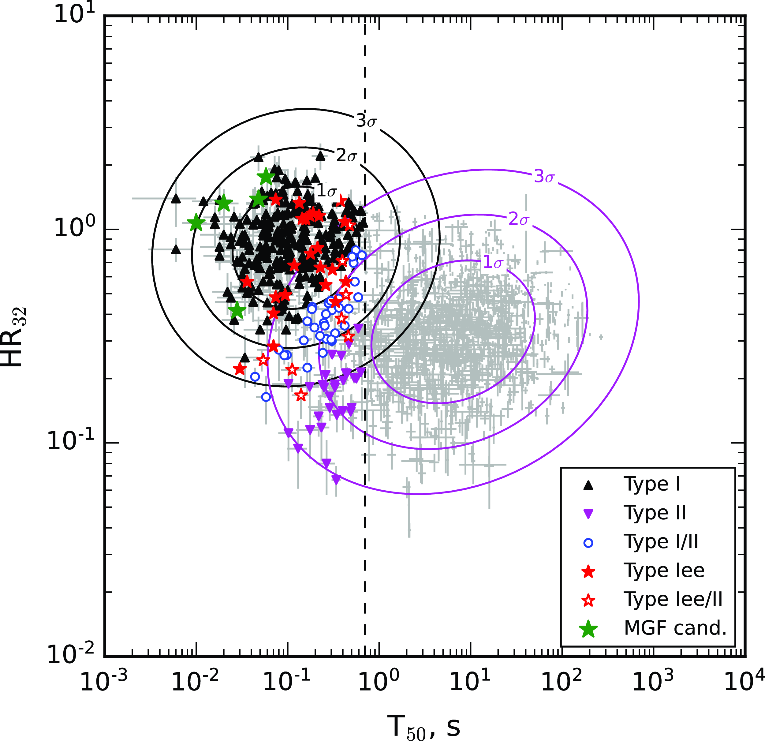
Figure 1. Hardness-duration distribution for 3398 KW GRBs. The distribution is fitted with a sum of two Gaussian distributions. The contours correspond to $1\sigma$ , $2\sigma$ , and $3\sigma$ cumulative probability for short-hard (black) and long-soft (magenta) distributions. The vertical dashed line denotes the boundary at $T_{50}$ = 0.7 s between short and long GRBs. The types for sGRBs are shown in colours: Type I (black triangles), Type I/II (blue circles), Type II (magenta inverted triangles), Type Iee (filled red stars), Type Iee/II (empty red stars), and MGF candidates (green stars). The remaining GRBs are plotted as grey crosses.

Hereafter we denote the KW sGRB sample detected in 1994–2010 as Sample I, the KW sGRB sample detected in 2011–2021 plus the recent MGF GRB 231115A as Sample II, and Sample I plus Sample II as the Full sGRB Sample.

We searched for sGRBs with EE candidates in Sample II using the criteria similar to those used in S16: a short ( $T_{50} \leq 0.7$ s) IP followed by a weaker emission without separate intense peaks and without prominent spectral evolution.

Table 1. KW sGRB Observation Details (Sample II).

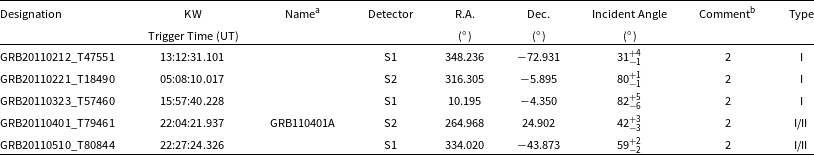
^aAs provided in the GCN circulars, if available.

^b1 – the burst was detected by an imaging instruments (the incident angle error is negligible and not given); 2 – the burst was localised by IPN; R.A. and Dec. correspond to the most probable source location; 3 – the burst was localised by IPN to a long segment, R.A. and Dec. are not given, the source ecliptic latitude estimate is used for the incident angle calculation; 4 – the burst was localised to a large region, R.A. and Dec. are not given, the incident angle is set at 60 $^{\circ}$ .

(This table is available in its entirety in machine-readable form.)

Table 2. Durations, Spectral Lags, and Classification (Sample II).

^aRelative to the trigger time.

(This table is available in its entirety in machine-readable form).

The bursts were classified into physical types using a two 2D Gaussian component fit to the hardness-duration distribution, in a way similar to S16, Tsvetkova et al. (2017) (hereafter T17), Svinkin et al. (2019), see Figure 1. Hereafter all Figures refer to the Full sGRB Sample. The burst spectral hardness, $HR_\mathrm{32}$ , was calculated using the ratio of counts in the G3 and G2 bands accumulated during the total burst duration ( $T_\mathrm{100}$ , see Section 4.1). The calculation of $HR_\mathrm{32}$ accounts for the KW gain drift (see S16). According to this classification, Sample II includes 152 Type I GRBs (merger origin; 76%), 22 Type II GRBs (collapsar origin; 11%), and for 17 sGRBs the type is uncertain (I/II; 8%). The classification of sGRBs that show extended emission was based on the IP parameters and yielded six Type I bursts with EE (Iee).

Burst localisation is essential for GRB spectral analysis, but KW has only a coarse autonomous localisation capability. In cases where the position of a GRB is not available from an imaging instrument (e.g., Swift-BAT), the source localisation can be derived using the InterPlanetary Network (IPN) triangulation (see, e.g., Hurley et al., 2013). The localisations of the KW sGRBs are reported in Pal’shin et al. (2013) and Svinkin et al. (2022).

Table 1 lists the 199 sGRBs of Sample II. The first column gives the burst designation in the form “GRBYYYYMMDD_Tsssss”, where YYYYMMDD is the burst date, and sssss is the KW trigger time $T_0$ (UT) truncated to integer seconds (note that due to Wind’s large distance from Earth, this trigger time can differ by up to $\sim 7$ s from the near-Earth instrument detection times; see Svinkin et al., 2022). The second column gives the KW trigger time in the standard time format. The “Name” column specifies the GRB name as provided in the Gamma-ray Burst Coordinates Network circulars ^c if available. The “Detector” column specifies the triggered detector. The columns “R.A.” and “Dec.” give sGRB localisation (see Footnote (b) to Table 1). The next column provides the angle between the GRB direction and the detector axis (the incident angle). The last but one column contains localisation-specific notes, and the last column specifies the burst type.

4. Data analysis and results

4.1. Durations and spectral lags

The burst durations $T_{100}$ (the total duration estimated using the threshold $5\sigma$ ), $T_{90}$ , and $T_{50}$ are calculated following the procedure described in Svinkin et al. (2019).

The spectral lag is a quantitative measure of the spectral evolution of GRBs. A positive lag corresponds to the delay of emission in a softer energy band relative to a harder one. It was shown that sGRBs both with and without EE have negligible spectral lag (Norris et al., 2001; Norris & Bonnell, 2006). Thus, the spectral lag can be used as an additional classification parameter.

We report spectral lags between light curves in the G2 and G1 ( $\tau_\mathrm{lag21}$ ), G3 and G2 ( $\tau_\mathrm{lag32}$ ), and G3 and G1 ( $\tau_\mathrm{lag31}$ ) energy bands. We calculated the lags using the cross-correlation function (CCF) similar to that used by Link et al. (1993), Fenimore et al. (1995), and Norris et al. (2000). We defined lag as the position of the maximum of the second-order polynomial fit to CCF near its peak. To estimate lag uncertainties, we used Monte Carlo simulations of the burst light curves in each energy band. For each simulation, we added Poisson noise to both light curves according to the count rates and calculated a spectral lag. The resulting lag was defined as the median of the simulated lag distribution, and the lag uncertainty was defined as the half-width of the 68% CL. For each burst, the time interval for cross-correlation, the temporal resolution of the light curve, and the CCF fitting interval were individually adjusted to account for the duration and the intensity of the event. For bursts with poor count statistics in one or two channels, the corresponding lags were not calculated. For bursts with EE, spectral lags were calculated for the IP only.

Figure 2. Spectral lag distributions. Left – distributions for Type I bursts (grey), Type I/II bursts (blue), Type II bursts (magenta), and MGF candidates (green). Right – distributions for Type I bursts (grey), Type Iee bursts (red), and Type Iee/II bursts (blue). In each column, the panels correspond to the following pairs of energy bands: G2 and G1 (top), G3 and G2 (middle), and G3 and G1 (bottom).

Table 2 contains the burst durations, the spectral lags, and the classification for Sample II. The first column gives the burst designation. The following four columns contain the start of the $T_{100}$ interval $t_0$ (relative to $T_0$ ), $T_{100}$ , $T_{90}$ , and $T_{50}$ . The next column gives the Type I–II classification, and the last three columns contain spectral lags $\tau_\mathrm{lag21}$ , $\tau_\mathrm{lag32}$ , and $\tau_\mathrm{lag31}$ .

Figure 2 presents the distributions of spectral lags. For Type I bursts the measured lags are distributed around zero, which is in agreement with the previous study (S16). We note that longer lags for Type I bursts tend to have large uncertainties (for a further discussion, see Section 5).

4.2. Minimum variability timescale, rise and decay times

To estimate the minimum variability timescale, rise, and decay times, we used the Bayesian block decomposition (Scargle et al., 2013) of the burst light curves. This decomposition segments a light curve into intervals (blocks), and within each block, the source count rate is assumed to be constant at a given significance level, with variations caused by random fluctuations ^d . We performed the segmentation on the sum of the observed count rates in the G2 and G3 channels at the significance level corresponding to $\sim 5\sigma$ . The minimum variability timescale $\delta T$ was evaluated for each burst as the duration of the shortest block. The peak time was defined as the centre time of the block with the maximum count rate. The rise time $\tau_\mathrm{rise}$ was estimated as the difference between the peak time and the beginning time of the first block of the burst, and the decay time $\tau_\mathrm{decay}$ – as the difference between the end time of the last block and the peak time. This approach, however, does not account for the multi-peaked structure observed for a number of sGRBs. For bursts, described with a single block, rise and decay times were not estimated.

Table 3. Minimum variability timescale, rise and decay times for the Full sGRB Sample

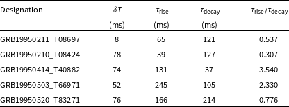
(This table is available in its entirety in machine-readable form).

Figure 3. Burst variability timescales derived for the G2+G3 channel light curves. The left column presents distributions for Type I bursts (grey), Type I/II bursts (blue), Type II bursts (magenta), and MGF candidates (green). The right column – distributions for Type I bursts (grey), Type Iee bursts (red), and Type Iee/II bursts (blue). Each row shows the distributions for the following parameters: (a) Minimum variability timescale $\delta T$ ; (b) Rise time $\tau_\mathrm{rise}$ ; (c) Decay time $\tau_\mathrm{decay}$ ; (d) Rise-to-decay time ratio.

Table 3 lists $\delta T$ , $\tau_\mathrm{rise}$ , $\tau_\mathrm{decay}$ , and the ratio $\tau_\mathrm{rise}$ / $\tau_\mathrm{decay}$ for the Full sGRB sample. Figure 3 presents distributions of these values for different sGRB types. The distribution of $\delta T$ peaks at $\sim 100$ ms and also has a minor separated peak at 2 ms. Given that 2 ms is the finest time resolution available for KW, this small peak corresponds to the bursts with $\delta T \le 2$ ms. The shortest $\delta T$ are typical for MGFs: three out of five MGFs have $\delta T \le 2$ ms. MGFs are also characterised by fast rise times: for three out of five bursts $\tau_\mathrm{rise}\lt 8$ ms. Fast time variability is typical for Type I and Type Iee bursts, while Type II bursts demonstrate significantly longer scales (for further discussion see Section 5).

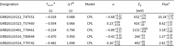
Table 4. Spectral Parameters (Multichannel Spectra) for Sample II.

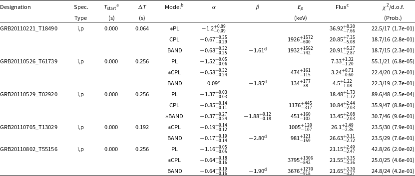
^aRelative to the trigger time.

^bThe best-fit model is indicated by the asterisk.

^cIn units of 10 $^{-6}$ erg cm $^{-2}$ s $^{-1}$ .

^dUpper limits.

^eLower limits.

(This table is available in its entirety in machine-readable form).

4.3. Spectral analysis

For a typical KW sGRB, the time-integrated (TI) spectrum may be well characterised using a subset of the first four 64 ms spectra measured from $T_0$ up to $T_0+0.256$ s. For some bright, relatively long events, we also include the 5th spectrum with an accumulation time of up to 8.192 s. The background spectrum for a burst without EE was usually taken starting from $\sim T_0+25$ s with an accumulation time of about 100 s. For about 53% of the bursts in Sample II, a major fraction of the total count fluence was accumulated before the trigger time and is not covered by the multichannel spectra. For these bursts, we use a three-channel spectrum constructed from the time-integrated light curve counts in G1, G2, and G3 (see S16).

We analysed a total of 94 multichannel and 105 three-channel TI spectra for Sample II. Due to low counting statistics of the majority of KW sGRBs, we typically use the burst TI spectrum to calculate its total energy fluence (S) and peak energy flux ( $F_\mathrm{peak}$ ). Only for 11 fairly intense GRBs it was possible to derive $F_\mathrm{peak}$ from a dedicated, “peak” spectrum covering a narrow time interval near the peak count rate.

We chose three spectral models to fit the spectra of GRBs from our sample. These models were a simple power law (PL), an exponential cutoff power law (CPL), and the Band’s GRB function (BAND; Band et al., 1993). All models are formulated in units of photon flux f (photon s $^{-1}$ cm $^{-2}$ keV $^{-1}$ ). The details of each model are presented below.

The power-law model

(1) \begin{equation}f_{\textrm{PL}} \propto E^{\alpha}\,.\end{equation}

The power-law with exponential cutoff

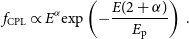(2) \begin{equation}f_{\textrm{CPL}} \propto E^{\alpha} {\textrm{exp}}\left(-\frac{E(2+\alpha)}{E_{\textrm{p}}}\right)\,.\end{equation}

The Band’s function:

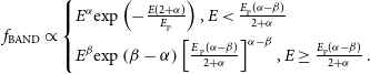(3) \begin{equation}f_{\textrm{BAND}} \propto\begin{cases}E^{\alpha} {\textrm{exp}}\left(-\frac{E(2+\alpha)}{E_{\textrm{p}}}\right), E\lt\frac{E_{\textrm{p}}(\alpha-\beta)}{2+\alpha} \\[5pt]E^{\beta} {\textrm{exp}}\left (\beta-\alpha \right) \left[ \frac{E_{\textrm{ p}}(\alpha-\beta)}{2+\alpha}\right]^{\alpha-\beta}, E \geq \frac{E_{\textrm{p}}(\alpha-\beta)}{2+\alpha}\,.\end{cases}\end{equation}

Here $E_{\textrm{p}}$ is the peak energy of the $EF_E$ spectrum, $\alpha$ is the low-energy photon index, and $\beta$ is the photon index at higher energies.

Spectral fitting was performed in XSPEC 12.11.1 package (Arnaud, 1996) using the $\chi^2$ statistics. For multi-channel spectra, to ensure the validity of the $\chi^2$ statistics, we grouped the energy channels to have at least 20 counts per channel. We used a model energy flux in the 10 keV–10 MeV band as the model normalisation during a fit. The flux was calculated using the cflux convolution model in XSPEC. The parameter errors were estimated using the XSPEC command error based on the change in the fit statistics ( $\Delta \chi^2 = 1.0$ ), which corresponds to 68% CL.

The preferred model (the best-fit model) between PL, CPL, and BAND was selected based on the F-test (Bevington, 1969). As in S16, a model with an additional parameter was selected as the best-fit model when the decrease in $\chi^2$ corresponds to the probability of chance decrease $\leq 0.025$ .

Table 5. Spectral Parameters (Three-channel Spectra) for Sample II.

^aThe burst start time relative to $T_{\textrm{0}}$ .

^bThe burst total duration $T_{\textrm{100}}$ .

^cIn units of 10 $^{-6}$ erg cm $^{-2}$ s $^{-1}$ .

(This table is available in its entirety in machine-readable form).

The three-channel spectra were analysed in a way similar to S16. In order not to overestimate the burst energetics, we limit the analysis to the CPL function. ^e Since the CPL fit to a three-channel spectrum has zero degrees of freedom, the parameter errors were estimated using the XSPEC steppar command. For the cases where $\alpha$ or $E_{\textrm{p}}$ were poorly constrained, typically, if $E_{\textrm{p}}$ is within G1 energy band or $E_{\textrm{p}}$ is above the three-channel analysis range (i.e., $\gtrsim 1$ MeV), we report the parameter lower (or upper) limits.

Figure 4. Distributions of $\alpha$ (left) and $E_{\textrm{p}}$ (right) obtained for GRBs with different best-fit models. Solid black lines – CPL fits to multi-channel spectra; dashed curves – CPL fits to three-channel spectra; the hatched histogram displays PL indices; dark grey histograms – the BAND model parameters. Light grey histograms show the summed-up distributions for all sGRBs.

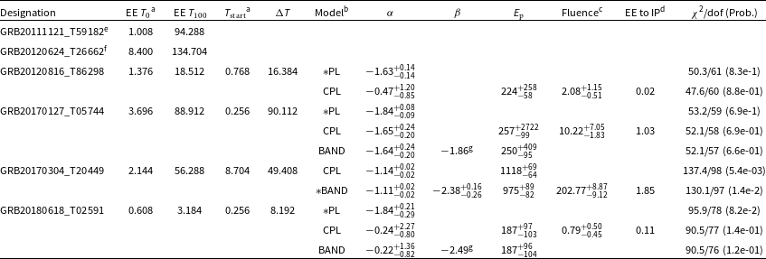
Table 4 provides the results of the multi-channel spectral analysis for the 94 TI spectra and the 11 spectra near the peak count rate of the Sample II bursts. The 10 columns in Table 4 contain the following information: (1) the burst designation (see Table 1); (2) the spectrum type, where ‘i’ indicates TI spectrum used to calculate the total energy fluence S; ‘p’ indicates that the spectrum is measured near the peak count rate (and is used to calculate the peak energy flux $F_\mathrm{peak}$ ), or ‘i,p’ – TI spectrum was used to calculate both S and $F_\mathrm{peak}$ ; columns (3) and (4) contain the spectrum start time $T_\mathrm{start}$ (relative to $T_0$ ) and its accumulation time $\Delta T$ ; column (5) lists models with the null hypothesis probabilities $P\gt10^{-6}$ for each spectrum, the best-fit model is indicated with the asterisks; columns (6)–(8) contain $\alpha$ , $\beta$ , and $E_\mathrm{p}$ ; column (9) represents the normalisation (energy flux in the 10 keV–10 MeV band); column (10) contains $\chi^2/\mathrm{dof}$ along with the null hypothesis probability P. In cases where the errors for $\beta$ are not constrained, we report the upper limit on $\beta$ . The 94 best-fit models for the TI spectra include 83 CPL, 9 BAND, and 2 PL.

Table 5 contains the results of the CPL fits for the 105 three-channel spectra of Sample II bursts. The seven columns contain the following information: column (1) gives the burst designation (see Table 1); columns (2) and (3) contain the spectrum start time $T_\mathrm{start}$ (relative to $T_0$ ) and its accumulation time $\Delta T$ ; column (4) provides the spectral model; columns (5) and (6) comprise $\alpha$ and $E_\mathrm{p}$ , respectively; column (7) presents the normalisation (energy flux in the 10 keV–10 MeV band).

Table 6. Fluences and Peak Fluxes (Sample II).

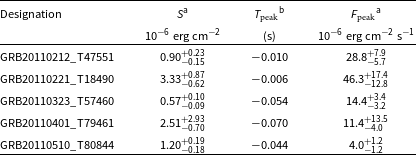
^aIn the 10 keV–10 MeV energy band.

^bRelative to the trigger time.

(This table is available in its entirety in machine-readable form).

The spectral parameter distributions for the Full sGRB Sample are presented in Figure 4. The distribution of $\alpha$ has a maximum at about −0.5 and spreads from $-2.0$ to $\sim 1.5$ . The maximum of the $E_{\textrm{p}}$ distribution lies between 400 and 500 keV, and the distribution extends over two orders of magnitude from a few tens of keV up to a few MeV. These results are in agreement with the results obtained in S16. ^f

Table 7. sGRBs with EE (Sample II).

^aRelative to the trigger time.

^bThe best-fit model is indicated by the asterisk.

^cIn units of $10^{-6}$ erg cm $^{-2}$ .

^dEE to IP fluence ratio.

^eEE was observed only in G1 channel, spectral fit is not feasible.

^fEE was observed only in G2 channel, spectral fit is not feasible.

^gUpper limits.

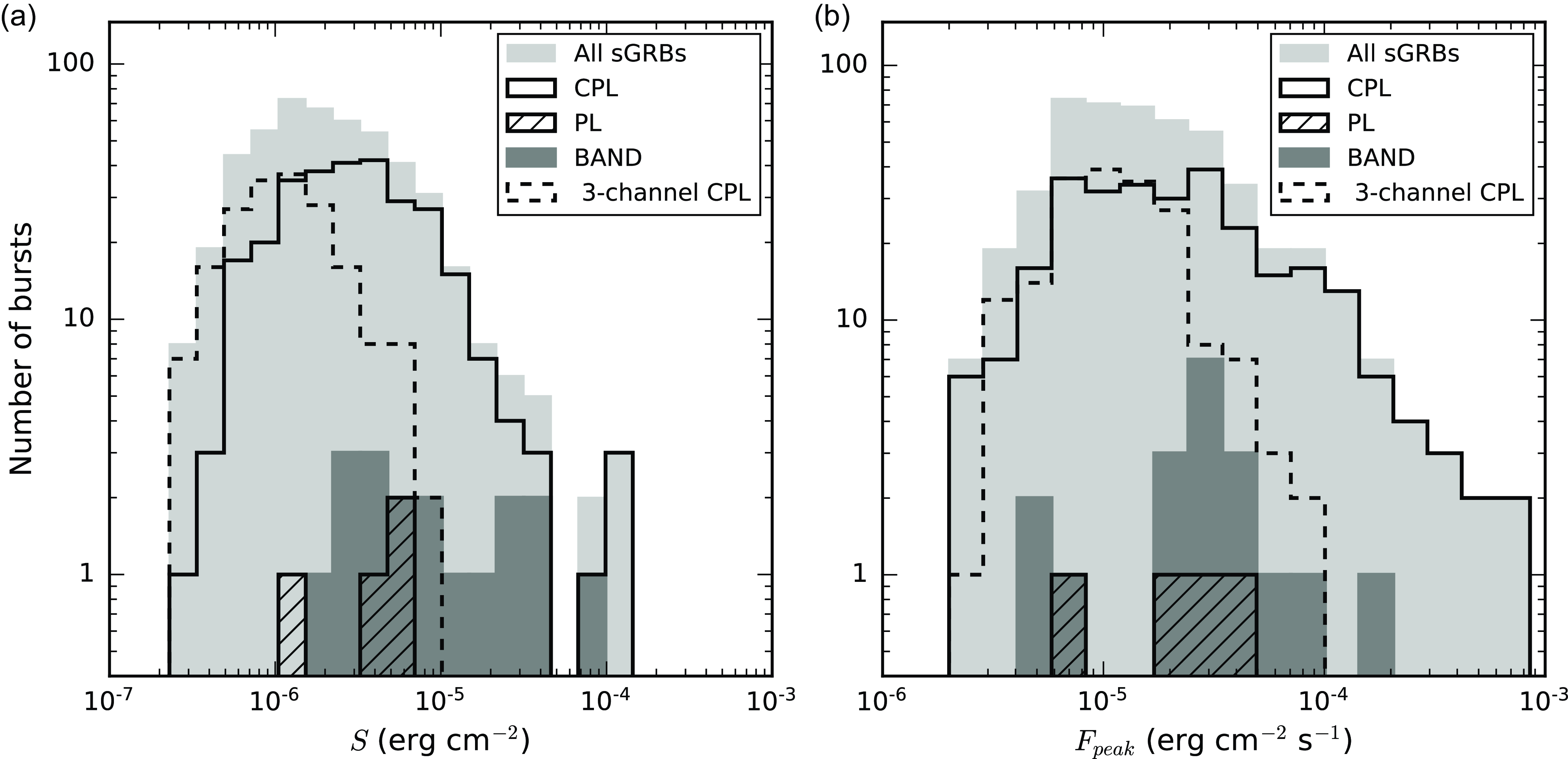
Figure 5. Fluence S (left) and peak flux $F_\mathrm{peak}$ (right) distributions. The light grey histogram corresponds to all sGRBs, the solid black curve represents sGRBs with multi-channel spectra fitted by a CPL model, the dashed black curve represents sGRBs with three-channel spectra, the hatched histogram corresponds to the PL model, and the dark grey histogram corresponds to the BAND model.

4.3.1 The peculiar GRB 111113A

For the intense GRB20111113_T18613 (GRB 111113A), the light curve consists of a single hard peak with a total duration of $\sim 160$ ms. There is a hint of a weaker emission starting $\sim 200$ ms before the main pulse and extending to $T_0+500$ ms. The burst spectrum demonstrates an excess above the hard CPL continuum ( $\alpha \sim -0.7$ , $E_p \sim 1500$ keV) at lower energies ( $\lesssim 50$ keV; Golenetskii et al., 2011). The spectral excess is well described by either a black-body component with the temperature $kT \sim 7.7$ keV or an additional PL component with the photon index $\sim 2.1$ . The blackbody and PL components contribute $\sim$ 1% and $\sim$ 8% to the 10 keV–10 MeV energy flux, respectively ( $7 \times 10^{-7}$ erg cm $^{-2}$ s $^{-1}$ for black-body and $3.6 \times 10^{-6}$ erg cm $^{-2}$ s $^{-1}$ for PL vs. $4.6 \times 10^{-5}$ erg cm $^{-2}$ s $^{-1}$ for CPL).

Table 8. Parameter distributions for different sGRB Types in the Full sGRB Sample. $^\mathrm{a}$

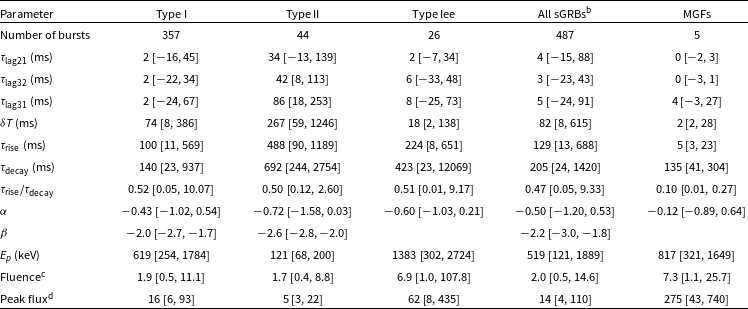
^aFor each parameter the median value is given, followed by the 90% CI in square brackets.

^bExcept MGFs.

^cIn units of $10^{-6}$ erg cm $^{-2}$ .

^dIn units of $10^{-6}$ erg cm $^{-2}$ s $^{-1}$ .

4.4. Fluences and peak fluxes

We derived S and $F_\mathrm{peak}$ using the normalising energy flux of the best-fit spectral model in the 10 keV–10 MeV band. In order not to overestimate the burst energetics, we used the CPL model for the cases where a divergent PL model (i. e., with $\alpha \gt -2$ ) was chosen as the best-fit model. Since the spectrum accumulation interval typically differs from the $T_{100}$ interval, a correction was introduced when calculating, S; for more details see S16 and T17.

$F_\mathrm{peak}$ was calculated as a product of the best-fit spectral model energy flux and the ratio of the 16 ms peak count rate to the average count rate in the spectrum accumulation interval. Typically, the peak count rate to the spectrum count rate ratio was calculated using counts in the G2+G3 light curve; the G1+G2, G2 only, and the G1+G2+G3 combinations were also considered depending on the emission hardness and signal-to-noise ratio.

For sGRBs with EE, S and $F_\mathrm{peak}$ of IP and EE were estimated independently.

Table 6 contains S and $F_\mathrm{peak}$ for the 199 bursts of Sample II. The first column gives the burst designation (see Table 1). The three subsequent columns give S; the start time of the 16 ms time interval, when the peak count rate in the G2+G3 band is reached; and $F_\mathrm{peak}$ .

The distributions of S and $F_\mathrm{peak}$ are shown in Figure 5. Both distributions extend over a few orders of magnitude (0.2–200) $\times 10^{-6}$ erg cm $^{-2}$ for S and (0.02–1000) $\times 10^{-5}$ erg cm $^{-2}$ s $^{-1}$ for $F_{\textrm{ peak}}$ . The S and $F_{\textrm{peak}}$ distributions peak at about $10^{-6}$ erg cm $^{-2}$ and $10^{-5}$ erg cm $^{-2}$ s $^{-1}$ , respectively.

4.5. sGRBs with EE

The parameters of the extended emission of six Sample II sGRBs are listed in Table 7. For four of these bursts the EE was intense enough to perform spectral fitting (see Section 4.3). The 12 columns of Table 7 contain the following information: (1) the burst designation; (2) the EE start time relative to $T_0$ ; (3) the EE total duration $T_{100, \mathrm{EE}}$ ; (4) the EE TI spectrum start time $T_{\textrm{start, EE}}$ and (5) its accumulation time $\Delta T$ ; (6) models with the null hypothesis probabilities $P \gt 10^\mathrm{-6}$ (the best-fit model is marked by an asterisk); (7)-(9) the model parameters: $\alpha$ , $\beta$ , $E_{\textrm{p}}$ ; (10) the energy fluence in the 10 keV–10 MeV range; (11) EE to IP fluence ratio; and (12) the $\chi^2$ /dof along with the null hypothesis probability. As for IPs, for the cases where a divergent PL model was chosen as the best-fit model, we used a CPL model for fluence calculation.

Three out of four bursts with constrained spectral fits are best described by PL and one – by BAND. For these models, the best-fit photon indices $\alpha$ are in the range between $-1.84$ and $-1.11$ . The peak energy of the EE fitted by BAND is rather hard, 975 keV, but this value is softer than that for the IP. For two bursts, the EE fluence is significantly smaller than that of the IP, and for the other two bursts, the EE fluence is comparable to the IP fluence.

In S16, 30 sGRBs with EE, or $\sim 10$ % of Sample I, were reported, among which 21 bursts were bright enough to produce reasonable spectral fits. In this work, for the more recent Sample II, we found only six (3%) bursts with EE. The lower fraction of bursts with EE in Sample II may be due to the shift of the KW energy range to higher energies, which makes rather faint and soft EE harder to detect.

Figure 6. Distributions of $\alpha$ and $E_{\textrm{p}}$ for TI spectra (upper panels) and peak spectra (lower panels) for different types. Left panels: Type I bursts (grey triangles), Type I/II bursts (empty blue circles), Type II bursts (magenta inverted triangles), Type II bursts from T17 (light magenta triangles), and MGF candidates (green stars). Right panels: Type Iee bursts (red stars), Type Iee/II bursts (empty red stars), and other types are shown in grey. Dotted and dashed vertical lines refer to the synchrotron fast-cooling and the synchrotron slow-cooling limit, respectively.

5. Discussion

5.1. Burst parameters and classification

We have presented the results of the systematic spectral and temporal analysis of 199 short GRBs, detected by KW during 2011–2021, which extends the KW sGRB sample to 494 events (1994–2021; in 27 years of operation). This implies the sGRB detection rate by KW of $\sim 19$ per year. Among GRB experiments (see Tsvetkova et al., 2022, for a recent review), the KW sGRB sample is one of the largest to date, Swift-BAT has detected 132 sGRBs up to August 2021 ^g ( $\sim 8$ per year; Lien et al., 2016), AGILE-MCAL has detected $\sim 220$ sGRBs from 2007 to 2020 ( $\sim 17$ per year; Ursi et al., 2022), and Fermi-GBM has detected $\sim 600$ up to 2021, August ^h ( $\sim 37$ per year; von Kienlin et al., 2020). In comparison with the Fermi-GBM sample, the KW bursts represent the brighter end of the sGRB population, with energy fluences above $0.3\times 10^{-6}$ erg cm $^{-2}$ in the 10 keV–10 MeV energy range.

Table 8 contains median values and 90% CIs of sGRB parameter distributions calculated for the Full sGRB Sample for different burst types: Type I, Type II, Type Iee, MGFs, and all sGRBs, excluding MGFs. Most Type I, Type Iee bursts and MGFs have negligible spectral lags within the uncertainties. MGFs differ from other sGRBs by considerably shorter $\delta T$ and $\tau_{\textrm{rise}}$ scales and a prominent asymmetry of the pulse profile that is characterised by a low $\tau_{\textrm{rise}}$ -to- $\tau_{\textrm{decay}}$ ratio. Type II bursts of our sample represent a tail of the whole Type II GRB population. They, unlike other types of sGRBs, display some typical properties of long GRBs, e.g., significant positive spectral lags and longer $\delta T$ scales.

In the lower section of Table 8, we characterise the spectral parameter distributions for the TI spectra. The median value of the photon index $\alpha$ for all sGRBs is close to $-1/2$ , and, within errors, only four sGRBs have $\alpha$ values steeper than $-3/2$ , violating the synchrotron fast-cooling limit (Preece et al., 1998). It should be noted that harder values of $\alpha$ tend to have larger fit uncertainties. For 160 sGRBs (32% out of Full sGRB Sample), 90% CI of $\alpha$ are above $-2/3$ , thus violating the synchrotron slow-cooling limit (Sari et al., 1998). Ten sGRBs, within uncertainties, are characterised by positive values of $\alpha$ , which can be related to the admixture of thermal emission to the synchrotron continuum (Axelsson et al., 2012; Burgess et al., 2015). The IPs of sGRBs with EE are in general harder spectrally and more intense as compared to the “genuine” Type I bursts. This may partly be due to a selection effect that results in the possible EEs of weaker Type I bursts being below the KW detection threshold.

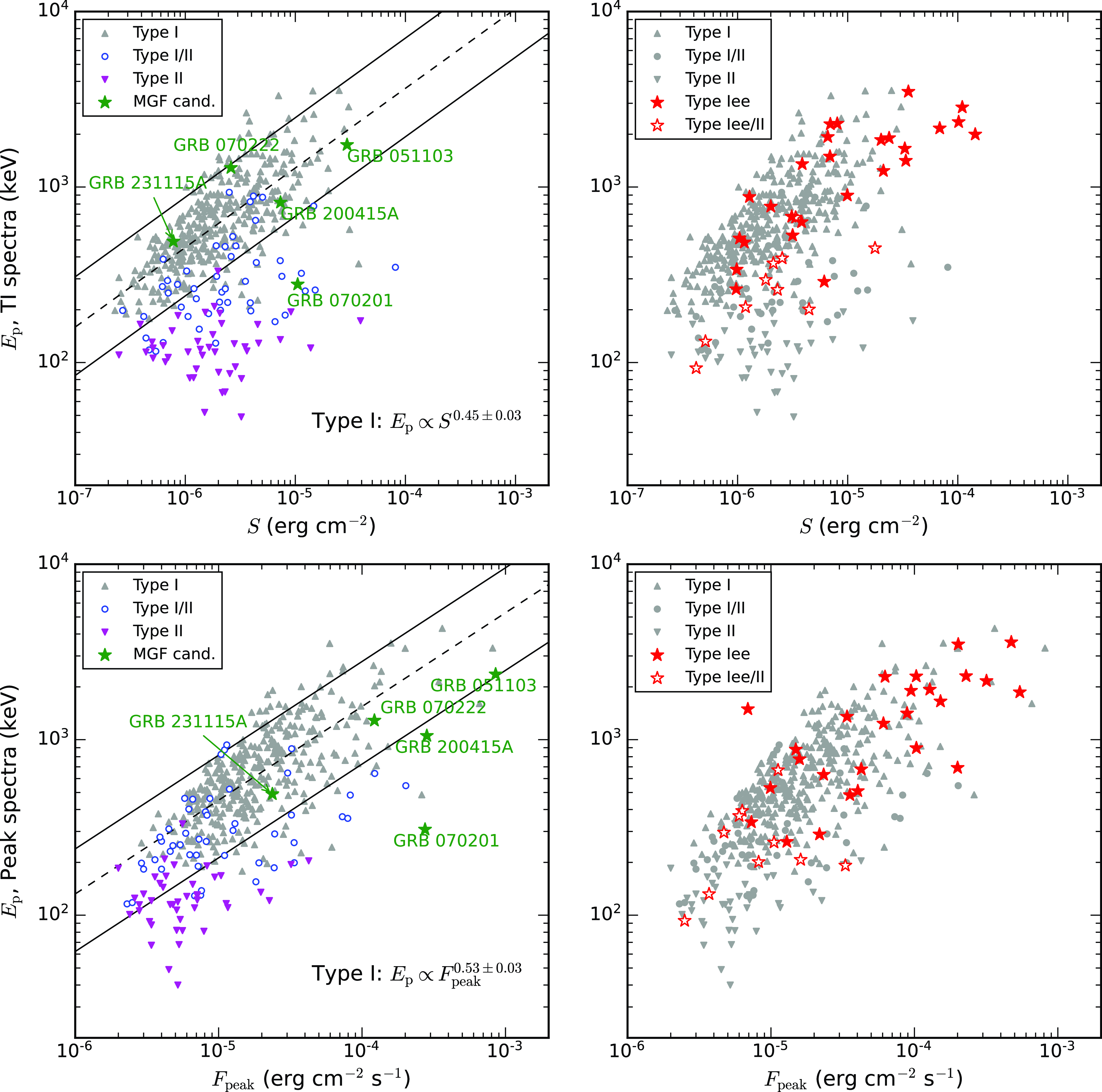
Figure 7. $E_{\textrm{p}}$ –S (upper panels) and $E_{\textrm{p}}$ – $F_{\textrm{peak}}$ (lower panels) distributions for different sGRB types. Left panels: Type I (grey triangles), Type I/II (empty blue circles), Type II (magenta inverted triangles), and MGF candidates (green stars); regressions for Type I bursts (black dashed line) and 90% PIs for Type I bursts (black solid lines). Right panels: Type Iee (red stars), Type Iee/II (empty red stars), and other types are shown in grey.

MGFs are characterised by higher $E_\mathrm{p}$ values and much higher $F_\mathrm{peak}$ than Type I bursts. For two MGFs (GRB 051103 and GRB 200415A), $\alpha$ of the TI spectra is close to zero, and one MGF (GRB 231115A) is characterised by a positive $\alpha$ value, which can be explained by a growing contribution of a thermal spectral component during the decaying phase of the burst (Svinkin et al., 2021). For two other MGFs (GRB 070201 and GRB 070222), $\alpha$ lies, within uncertainties, between fast- and slow- synchrotron cooling limits.

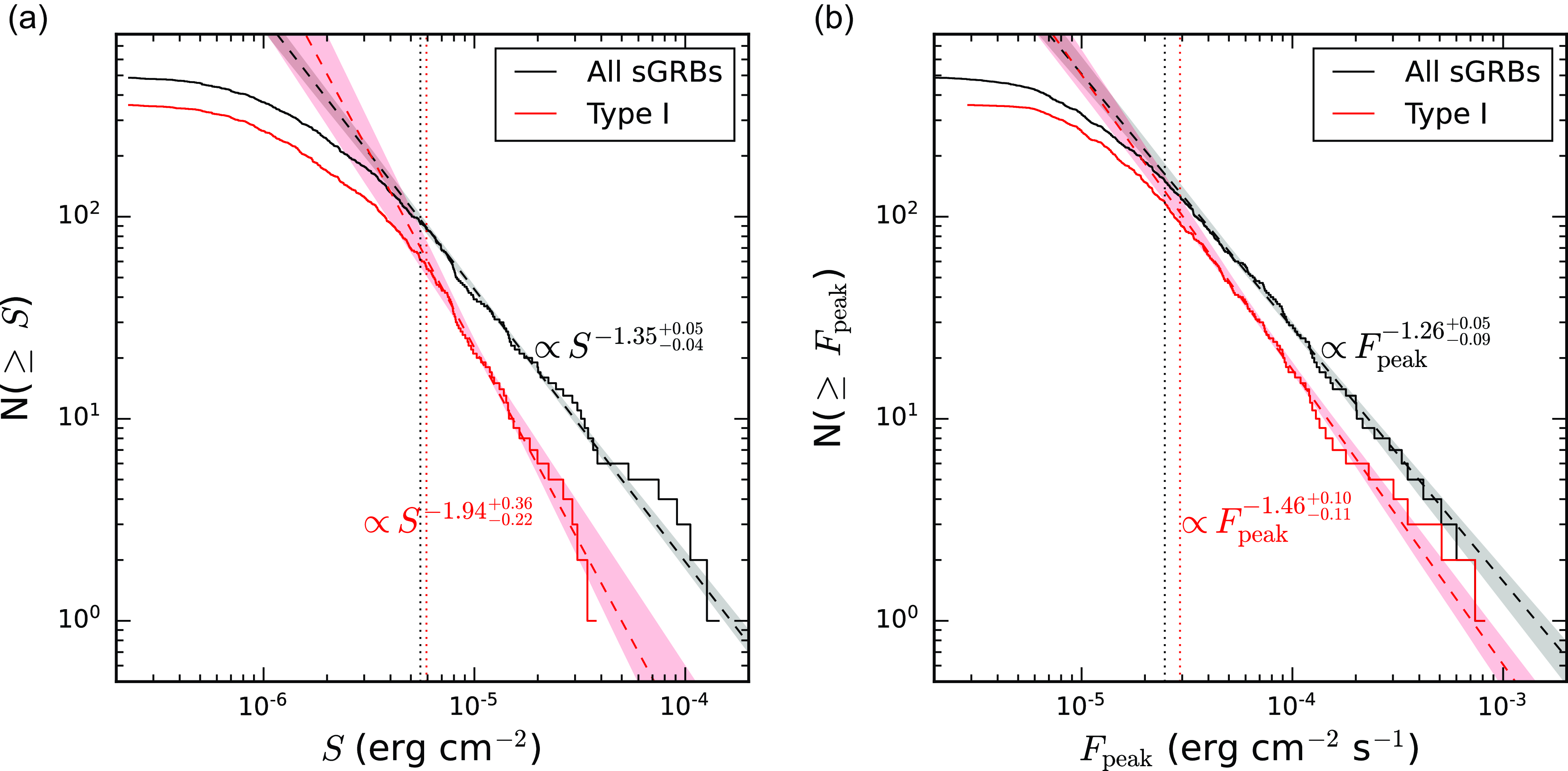
Figure 8. Cumulative distributions of the total energy fluence (left panel) and the peak energy flux (right panel). In both panels, black and red histograms represent cumulative distributions for the whole sGRB sample and for the Type I GRB sub-sample, respectively. Dashed lines indicate PL fit to the distributions for all sGRBs (black) and Type I bursts (red). Dotted vertical lines mark the left boundaries of the ranges, where the assumption that the data are PL-distributed is valid. Grey and pink areas on both plots indicate 68% CI for PL fit for all sGRBs and Type I bursts, respectively.

The majority ( $\sim 92$ %) of sGRBs with multi-channel spectra are best-fitted by CPL, while BAND is the best-fit model only for 18 out of 308 ( $\sim 6$ %) bursts with multi-channel spectra. Among the latter bursts there are nine Type I bursts, four Type II bursts, three Type I/II bursts, one Type Iee burst, and the MGF candidate GRB 051103. The low fraction of BAND spectra, as compared to the long GRB population (e.g., $\sim$ 38% in the T17 sample), could be attributed to relatively poor count statistics in short bursts that do not allow to constrain properly their spectral shapes at higher energies. On the other hand, the cutoff spectra could be a distinct feature of merger-origin GRBs. Recently, a number of long GRBs have been confirmed to originate from compact object mergers, which underlines the ambiguity of GRB classifications based on duration only. For at least one of them, the ultra-bright GRB 230317A, accompanied by a kilonova (Levan et al., 2024), high signal-to-noise spectra are best described by CPL during the whole main emission phase (Svinkin, D. S., et al., in preparation). Thus, the statistically significant exponential cut-off at higher energies may point to the merger origin for some long-duration GRBs.

Figure 6 presents 2D distributions of $\alpha$ and $E_{\textrm{p}}$ for different GRB types, including Type II bursts from T17. The general form of the distributions is similar to that reported by Poolakkil et al. (2021) for GRBs detected by Fermi-GBM. It should be noted that the spectra with lower $E_{\textrm{p}}$ values tend to have larger uncertainties in $\alpha$ , which may explain the increase in the width of the index distribution with decreasing $E_{\textrm{p}}$ . The $\alpha$ – $E_{\textrm{p}}$ distributions for IPs of sGRBs with EE are generally consistent with those for Type I bursts. A vivid difference is observed between Type I and Type II bursts: Type II bursts have, in general, lower $E_{\textrm{p}}$ values than Type I bursts and are characterised by significantly softer $\alpha$ indices for both TI and peak spectra. As with the hardness-duration relation, there is no distinct boundary between GRBs of different Types in the $\alpha$ – $E_{\textrm{p}}$ plane, but the typical parameter values for Type I GRBs in this plane tend to be different from those for Type II bursts. To compare the burst distributions in the $\alpha$ – $E_{\textrm{p}}$ plane, we applied the bivariate Kolmogorov-Smirnov test (2D KS-test, Peacock, 1983; Fasano & Franceschini, 1987; Press et al., 1992). We found that the probability that $\alpha$ – $E_{\textrm{p}}$ distributions are similar for Type I and Type II bursts is negligible ( $P\lt10^{-20}$ ), while the distributions for Type I bursts and Type Iee bursts are rather consistent: 2D KS-test results in probability $P= 6 \times 10^{-3}$ for TI spectra and $P= 3 \times 10^{-2}$ for peak spectra.

Figure 7 shows $E_{\textrm{p}} - S$ and $E_{\textrm{p}} - F_\mathrm{peak}$ relations for the Full sGRB Sample. To estimate slopes m (i.e., $E_{\textrm{p}} \propto S^m$ ) for these relations, we used the fitting method with bivariate correlated errors and intrinsic scatter (BCES, Akritas & Bershady, 1996) realised in Python (Nemmen et al., 2012). For Type I bursts we found $E_{\textrm{p, I}} \propto S_{\textrm{I}}^{0.45 \pm 0.03}$ and $E_{\textrm{p, I}} \propto F_{\textrm{peak, I}}^{0.53 \pm 0.03}$ . Type II sGRBs, which represent a low-intensity fraction of the long-soft GRB population, lie below the lower bound of the 90% prediction interval (PI) of the $E_{\textrm{p}} - S$ relation for Type I sGRBs. This result is consistent with studies of GRB rest-frame properties (T17; Zhang et al., 2018; Minaev & Pozanenko, 2020; Tsvetkova et al., 2021), which demonstrate that populations of Type I and Type II GRBs occupy different regions in the intrinsic $E_\mathrm{p}$ – isotropic burst energy release ( $E_\mathrm{iso}$ ) plane.

Four out of five MGF candidates fall into or are very close to the 90% PI on both the $E_{\textrm{p}}$ –S and $E_{\textrm{ p}}$ – $F_{\textrm{peak}}$ planes. The remaining MGF candidate, GRB 070201, is an outlier with much lower peak energy as expected for Type I bursts. Two right panels of Figure 7 show the 2D parameter distributions for IPs of sGRBs with EE. For Type Iee bursts the distributions do not differ significantly from those for genuine Type I GRBs.

5.2. sGRB energetics and spatial distribution

Figure 8 presents the cumulative distributions of fluences and peak fluxes for Full sGRB Sample (excluding MGF candidates) and Type I subsample. Due to various instrumental biases, which result in the lack of the faint bursts in the sample, both logN–logS and logN–log $F_{\textrm{peak}}$ distributions follow a PL in a limited range of fluences and peak fluxes. We used the powerlaw Python package (Alstott et al., 2014) both for the determination of the range where a PL is valid and for the estimation of the PL slope $\gamma$ . We performed Monte-Carlo simulations of multiple S and $F_{\textrm{peak}}$ sets; for each set, we estimated the range for PL and PL slope. The resulting slope was taken as the median value for all simulated sets, and the 68% CI for the slope was estimated.

The logN–logS distribution for all sGRBs follows a PL for fluences $\gtrsim 5 \times 10^{-6}$ erg cm $^{-2}$ , with the slope $\gamma_{\textrm{all, S}}=-1.35_{-0.04}^{+0.05}$ . The obtained slope is flatter than −3/2 (the slope for homogeneously distributed sources), which is expected for red-shifted sources (Meegan et al., 1992). The distribution for Type I bursts only obeys a PL for fluences above $\sim 6 \times 10^{-6}$ erg cm $^{-2}$ , with the slope $\gamma_{\textrm{I, S}}=-1.94_{-0.22}^{+0.36}$ , which is steeper than expected for homogeneously distributed sources. The lack of high-fluence Type I sources can be related to the absence of Type I bursts with longer durations in our sample. Some of such longer Type I GRBs lie within the short-hard GRB cluster but do not obey our criterion of short bursts, and some merger-origin GRBs could, in fact, be long GRBs (see, e.g., Petrosian & Dainotti, 2024). For the logN–log $F_{\textrm{peak}}$ distribution, a PL is applicable for the peak fluxes $ \gtrsim 2 \times 10^{-5}$ erg cm $^{-2}$ s $^{-1}$ for all sGRBs and $ \gtrsim 3 \times 10^{-5}$ erg cm $^{-2}$ s $^{-1}$ for Type I bursts. The PL slopes constitute $\gamma_{\textrm{all, F}}=-1.26_{-0.09}^{+0.05}$ for all sGRBs and $\gamma_{\textrm{I, F}}=-1.46_{-0.11}^{+0.10}$ for Type I bursts. The value of $\gamma_{\textrm{I, F}}$ is close to −3/2, which is related to low redshifts of Type I bursts.

6. Summary and conclusions

In this catalogue, we analyse the temporal and spectral characteristics as well as energetics of 199 sGRBs, detected by KW between 1 January 2011 and 31 August 2021. Together with the Second Catalogue, the total KW sGRB sample comprises 494 sGRBs detected in 1994-2021 and the recent MGF candidate GRB 231115A. For the whole set of 494 sGRBs, we presented statistical distributions of spectral lags, minimum variability timescales, rise and decay times, spectral fitting parameters, energy fluences, and peak energy fluxes. We compared distributions of these characteristics for different sGRB subsamples: Type I (merger-origin), Type II (collapsar-origin), Type Iee (merger-origin bursts with extended emission), and MGF candidates. We found that MGF candidates differ from other sGRBs by shorter variability timescales and rise times and the higher asymmetry of the emission pulse. Type Iee burst IPs demonstrate properties similar to genuine Type I bursts, suggesting these bursts represent the more intense and spectrally hard fraction of the Type I population. Compared to other sGRBs from our sample, Type II bursts are characterised by significant positive spectral lags, longer variability timescales, and softer energy spectra, all of which are typical of long GRBs of collapsar origin.