Biophysical and chemical factors governing picophytoplankton succession in the Indian sector of the Southern Ocean during austral summer

Abstract

The Southern Ocean, a region characterized by high nutrient levels but often low productivity, hosts dynamic picophytoplankton communities crucial for its food web. This study investigated the spatial and inter-annual variability of picophytoplankton abundances and their environmental drivers in the Indian sector of the Southern Ocean during the austral summers of 2018 and 2020. Using flow cytometry for picophytoplankton quantification and standard oceanographic methods for environmental parameters (temperature, salinity, nitrate, phosphate, silicate), we employed descriptive statistics, inferential group comparisons (t-tests, analysis of variance), principal component analysis (PCA) and principal component regression (PCR) to analyse the dataset. Our analyses revealed significant differences in picophytoplankton abundances and environmental conditions across distinct oceanic fronts, between deep chlorophyll maximum and surface depths and, notably, between the two study years. PCA identified three major environmental gradients explaining over 93.5% of the variance in temperature, salinity, nitrate, phosphate and silicate. PCR confirmed our hypothesis: the abundance and carbon biomass of picoeukaryote II (PEUK-II) picophytoplankton was statistically significant overall (F-statistic = 3.415, P = 0.0290). The model explained 24.2% of the variance in PEUK-II abundance (R² = 0.242), indicating its sensitivity to dynamic oceanographic conditions, with PC3 (primarily representing a salinity gradient) being a significant predictor. Conversely, Prochlorococcus-like/Synechococcus picophytoplankton abundance was not statistically significant overall (F-statistic = 2.068, P = 0.124), suggesting control by other, potentially non-linear factors. These findings highlight distinct ecological strategies among picophytoplankton groups and are vital for predicting their roles in the Southern Ocean’s microbial food web amidst ongoing environmental change.

Introduction

The Southern Ocean, including its Indian sector, is often characterized as a region of paradox: high nutrient levels coexist with generally low biomass and productivity (Chapman et al. 2020). This dynamic environment is further shaped by distinctive hydrological fronts, which delineate varying hydrological, chemical and biological features, playing a crucial role in determining the spatial heterogeneity and dynamics of plankton populations (Thomalla et al. 2023). While large-size diatoms have traditionally been considered the primary foundation of the Antarctic food web, recent research has significantly revised this classical concept, increasingly emphasizing the importance of picoplanktonic organisms across diverse regions of the Southern Ocean (Wright et al. 2009).

Picophytoplankton, defined by their minute cell sizes ranging between 0.2 and 2.0 μm in diameter, are recognized as fundamental components of marine ecosystems globally. This diverse group encompasses picocyanobacteria, such as Prochlorococcus and Synechococcus, alongside various picoeukaryotes. While Prochlorococcus is prevalent in tropical and subtropical open oceans, Synechococcus exhibits a broader geographical distribution, extending into polar and high-nutrient regions (Johnson et al. 2006, Li 2009). Picoeukaryotes, often classified into distinct groups (e.g. PEUK-I and PEUK-II), and Synechococcus are particularly prolific in coastal and even eutrophic waters, underscoring their vital function in global carbon cycling and overall ecosystem processes (Li 2009). Flow cytometry offers a precise and quantitative method for assessing the cell densities and assemblage compositions of these major groups in the open ocean (Chisholm et al. 1988).

Numerous studies have highlighted the ubiquitous nature of these organisms and their significant contributions to primary production across various marine environments (Wright et al. 2009). In the Southern Ocean, they play an important part in both phytoplankton biomass and production, providing a seasonally stable pool of cells crucial for food web maintenance (Murphy et al. 2007, Saba et al. 2014, Liang et al. 2017). However, despite their ecological importance, the specific ecophysiological capabilities and the precise environmental conditions governing their distribution in these dynamic high-latitude systems remain poorly understood. While Antarctic research has often focused on regional variations, there is a notable lack of comprehensive documentation on the spatial and inter-annual changes in their composition and controlling factors, especially outside coastal areas (Garrison et al. 2000, Morin & Thiller 2009, Lin et al. 2012).

This study aims to address these gaps by providing a detailed characterization of the spatial variability in picophytoplankton communities in the Indian sector of the Southern Ocean during the austral summer (December–February). Data were collected along a transect between meridians 57°E and 81°E, spanning from the vicinity of the Subtropical Front (STF; ~39°S) to coastal Antarctica (~68°S). Furthermore, this research extends beyond single-year observations by comparing results obtained during the austral summers of 2018 (SOE10) and 2020 (SOE11) along the same transect, thereby assessing inter-annual variability. Based on the complex interplay of environmental influences in this region, we hypothesize that the abundance of specific groups, such as PEUK-II, is significantly explained by major hydrochemical gradients (e.g. principal components representing variations in temperature, salinity, nitrate, phosphate and silicate concentrations), while the abundance of others, such as Prochlorococcus-like/Synechococcus (PRO-like/SYN-PC), is not linearly driven by these same dominant parameters. Understanding these relationships is critical for predicting the future distribution and ecological functions of picophytoplankton under ongoing global environmental changes.

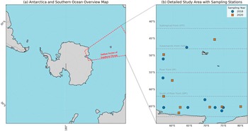
Figure 1. Map of the study area in the Indian Sector of the Southern Ocean, showing a. an overview of Antarctica and the Southern Ocean and b. detailed sampling stations for the 2018 and 2020 expeditions with approximate oceanic front boundaries.

Materials and methods

Study area and sampling

The study was conducted during two Indian Southern Ocean Expeditions (SOE10 and SOE11) onboard the research vessel SA Agulhas. Fieldwork took place during the austral summers of 2018 and 2020. The observational transect lay within the Indian sector of the Southern Ocean, spanning between meridians 57°E and 81°E, from the vicinity of the STF (~39°S–44°S), the Sub-Antarctic Front (SAF; ~45°S–49°S), the Polar Front (PF; ~50°S–58°S) and south of the Polar Front (SPF; ~59°S–68°S) southwards to coastal Antarctica (Orsi et al. 1995, Anilkumar et al. 2006). A map illustrating the locations of all stations from both cruises is provided in Fig. 1. At each designated site, water was collected from various depths using a conductivity-temperature-depth (CTD) rosette sampler equipped with Niskin bottles. Salinity (practical salinity units; PSU) and temperature (°C) profiles were continuously recorded by the onboard CTD system during collection.

Environmental data collection

Concentrations of dissolved inorganic nutrients, including nitrate (NO₃^-), phosphate (PO₄^3-) and silicate (SiO₄⁴), were analysed from collected water samples using an auto-analyser (Seal Analytical AA3) following standardized methods (Grasshoff et al. 1983). Three to four litres of water samples were filtered using GF/F Whatman filters, with the volume adjusted based on cell concentration density, to measure the chlorophyll a (chl a) concentration. The resulting filtrates were frozen at -20°C until analysis. Pigments were then extracted from the filters using 90% acetone, and the chl a biomass was quantified using a Turner’s AU 10 Fluorometer from Turner Designs, Inc. (USA), following the methodology outlined by Parsons et al. (2013).

Picophytoplankton sample collection and flow cytometry analysis

Samples for picophytoplankton analysis were carefully preserved immediately upon collection by adding paraformaldehyde to a final concentration of 0.2%. They were then flash-frozen in liquid nitrogen and stored at −80°C until laboratory analysis. The abundance and community structure of picophytoplankton were determined at an onshore laboratory using a BD FACS Melody™ flow cytometer (Becton Dickinson, USA). Prior to analysis, samples were pre-filtered through a 50 μm mesh to remove larger particles, and a 4 ml subsample was used for each measurement. Then, 2 μm Fluoresbrite® YG microspheres (Polysciences, USA) were added to each subsample as internal standards for instrument calibration and cell size referencing.

The flow cytometer, equipped with blue (488 nm) and red (633 nm) lasers, was used to excite cellular pigments. The blue laser excited chlorophyll and phycoerythrin, with red and orange fluorescence detected accordingly. The red laser specifically excited phycoerythrin, and its fluorescence emission was also recorded. Picophytoplankton populations were differentiated and quantified based on their fluorescence characteristics and light scatter signals (forward-angle scatter (FSC) and side scatter) following established protocols (Balfoort et al. 1992).

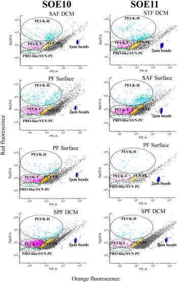
Typical flow cytometry plots illustrating the picophytoplankton populations and their optical properties are shown in Fig. 2. Based on unique fluorescence and scatter signatures, the populations were categorized into major groups: picoeukaryotes (PEUK), showing strong red fluorescence and relatively larger sizes, further subdivided into PEUK-I and PEUK-II; Synechococcus with phycoerythrin (SYN-PE), characterized by orange fluorescence and smaller size; and a PRO-like/SYN-PC cluster, exhibiting low red fluorescence and small size. At lower latitudes along the transect, this group showed optical features consistent with Prochlorococcus (e.g. FSC patterns relative to the 2 μm beads), while also including low-phycoerythrin Synechococcus strains. Hence, they were collectively designated as PRO-like/SYN-PC.

Figure 2. Typical flow cytometer histograms/graphs depicting the picophytoplankton communities (Synechococcus with phycoerythrin (SYN-PE), Prochlorococcus-like/Synechococcus (PRO-like/SYN-PC), picoeukaryotes (PEUK-I, PEUK-II)) in the Indian sector of the Southern Ocean during the austral summers of 2018 and 2020. These results were collected from random stations, covering various fronts, along with surface and deep chlorophyll maxima (DCM) water samples. The black-coloured points, appearing as a single line of mass (not scattered or forwarded), are considered debris of the community. PE-A = phycoerythrin area; PerCP-A = peridinin-chlorophyll protein area; PF = Polar Front; SAF = Sub-Antarctic Front; SOE = Southern Ocean Expedition; SPF = south of the Polar Front; STF = Subtropical Front.

Picophytoplankton carbon biomass estimation

The carbon biomass for each of the identified picophytoplankton groups was estimated by converting their cell abundance using established conversion factors: 250 fg/cell for Synechococcus, 53 fg/cell for Prochlorococcus and 2100 fg/cell for picoeukaryotes (Lee & Fuhrman 1987, Campbell et al. 1994, Buck et al. 1996, Garrison et al. 2000).

Statistical analysis

All statistical analyses were conducted using Python (version 3.12), incorporating the pandas, numpy, scipy, statsmodels and scikit-learn libraries. Prior to analysis, missing values in the environmental and picophytoplankton datasets were imputed using the column means. Basic descriptive statistics (e.g. mean, standard deviation, range) were computed to summarize the distributions of environmental parameters and picophytoplankton abundances.

For inferential comparisons, independent-samples t-tests were used to evaluate significant differences in picophytoplankton concentrations and environmental metrics between two groups (e.g. deep chlorophyll maximum (DCM) vs surface depths, or pairwise comparisons across oceanic fronts). One-way analysis of variance (ANOVA) was used to assess variations across more than two categories, such as among fronts or between study years. Where ANOVA yielded significant results, Tukey’s Honestly Significant Difference (HSD) post hoc test was applied to identify pairwise disparities.

To explore relationships between environmental factors and picophytoplankton groups, Pearson correlation coefficients were computed and visualized as heatmaps. Principal component analysis (PCA) was applied to standardized environmental variables (temperature (°C), salinity (PSU), nitrate, phosphate and silicate in μmol l⁻¹) to identify key gradients and reduce dimensionality. Standardization via StandardScaler ensured equal weighting across variables with different scales. The resulting components and their loadings were interpreted in order to understand dominant environmental influences.

To examine multivariate associations while addressing multicollinearity, principal component regression (PCR) was performed. The top three principal components (PC1, PC2, PC3), which together explained over 90% of the variance, were used as predictors in separate ordinary least squares (OLS) regression models for PEUK-II and PRO-like/SYN-PC abundances. Model performance (F-statistic, R ²) and the significance of individual component coefficients (P-values) were evaluated. A low condition number in the PCR models confirmed effective mitigation of multicollinearity.

Results

Descriptive statistics and overall data characteristics

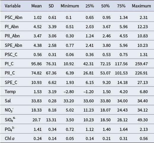
Environmental variables across the sampled stations exhibited broad gradients in temperature (−1.75°C to 9.96°C) and nutrient availability, reflecting the influence of multiple water masses and frontal zones encountered along the transect (Table I). Salinity remained relatively stable (33.30–34.48), consistent with typical Antarctic surface waters. Nutrient levels were elevated, with nitrate reaching 40.01 μmol l⁻¹, silicate up to 74.55 μmol l⁻¹ and phosphate ranging from 0.74 to 2.40 μmol l⁻¹, characterizing the high-nutrient, low-chlorophyll conditions of the region.

Table I. Overall descriptive statistics of picophytoplankton groups and environmental variables (n = 36).

SD = standard deviation; PSC = Prochlorococcus-like/Synechococcus (PRO-like/SYN-PC); PI = PEUK-I; PII = PEUK-III; SPE = Synechococcus with phycoerythrin (SYN-PE); Abn = abundance (cells × 10⁷ l⁻¹); C = carbon (pg C cell⁻¹); Temp = temperature (°C); Sal = salinity (PSU); NO₃^- = nitrate (μmol l⁻¹); SiO₄^4- = silicate (μmol l⁻¹); PO₄^3- = phosphate (μmol l⁻¹); Chl a = chlorophyll a (μg l⁻¹).

Picophytoplankton showed marked spatial variability. Synechococcus-like cells were numerically dominant (mean: 3.68 × 10⁷ cells l⁻¹) and also contributed the highest mean carbon biomass (5.54 μg C l⁻¹), while picoeukaryotes, despite lower cell numbers, exhibited higher per-cell carbon contents. Prochlorococcus-like cells were less abundant overall. High coefficients of variation in both abundance and biomass underscore the heterogeneity of picophytoplankton communities across different stations and depths.

Inferential group comparisons

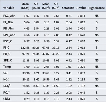
Vertical distribution: deep chlorophyll maximum vs surface depths

Independent-samples t-tests revealed significant differences in several picophytoplankton and environmental variables between samples collected at the DCM and the surface. Both the abundance and carbon biomass of picoeukaryotes (PEUK-I and PEUK-II) were significantly higher at DCM depths (P < 0.05 for all comparisons). For instance, mean PEUK-I abundance at DCM was 5.84 × 10⁷ cells l⁻¹, compared to 3.19 × 10⁷ cells l⁻¹ at the surface.

In contrast, no significant differences were observed in the abundance or biomass of Synechococcus (SYN-PE) and PRO-like/SYN-PC between these depth layers (P > 0.05; Fig. S1). Among environmental parameters, salinity, phosphate and chl a concentrations were significantly higher at the DCM, whereas temperature, nitrate and silicate showed no significant variation between depths (P > 0.05; Table II & Fig. S2).

Table II. Independent-samples t-test results comparing deep chlorophyll maximum (DCM) and surface depths (n = 18 per depth).

SD = standard deviation; PSC = Prochlorococcus-like/Synechococcus (PRO-like/SYN-PC); PI = PEUK-I; PII = PEUK-III; SPE = Synechococcus with phycoerythrin (SYN-PE); Abn = abundance (cells × 10⁷ l⁻¹); C = carbon (pg C cell⁻¹); Temp = temperature (°C); Sal = salinity (PSU); NO₃^- = nitrate (μmol l⁻¹); SiO₄^4- = silicate (μmol l⁻¹); PO₄^3- = phosphate (μmol l⁻¹); Chl a = chlorophyll a (μg l⁻¹); NS = not significant; S = significant (P < 0.05).

Spatial variability: oceanic fronts

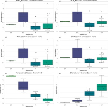
One-way ANOVA revealed significant differences in the abundance and carbon biomass of picoeukaryotes (PEUK-II) and Synechococcus (SYN-PE) across distinct oceanic fronts: STF, SAF, PF and SPF (P < 0.05; Figs 3 & S4–S7). Post-hoc Tukey’s HSD tests (Table S1) indicated that PEUK-II abundance and biomass were significantly higher at the SAF compared to the PF (P < 0.05), as were SYN-PE abundance and biomass. No other significant pairwise differences were observed among the fronts for these groups. Among the environmental parameters, significant overall differences were found for temperature and silicate across the fronts (P < 0.001). Tukey’s HSD results revealed multiple significant pairwise differences, with temperature differing between nearly all frontal zones, and silicate showing significant contrasts between PF and SAF, PF and SPF, PF and STF, and SAF and SPF. In contrast, salinity, nitrate, phosphate and chl a did not exhibit significant differences across the oceanic fronts (P > 0.05).

Figure 3. Box plots illustrating the spatial variability of picoeukaryotes (PEUK-II) and Synechococcus with phycoerythrin (SYN-PE) abundance and carbon biomass, as well as temperature and silicate variables, across distinct oceanic fronts (Sub-Antarctic Front (SAF), Polar Front (PF), south of the Polar Front (SPF) and Subtropical Front (STF)).

Inter-annual variability: 2018 vs 2020

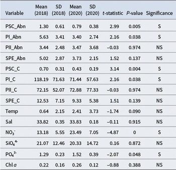
Independent-samples t-tests were conducted to compare variables between the 2018 (SOE10) and 2020 (SOE11) expeditions. Both the abundance and carbon biomass of PRO-like/SYN-PC and PEUK-I were significantly higher in 2018 than in 2020 (P < 0.05). For instance, the mean PRO-like/SYN-PC abundance was 1.30 × 10⁷ cells l⁻¹ in 2018, compared to 7.94 × 10⁶ cells l⁻¹ in 2020. No significant differences were observed for PEUK-II or SYN-PE abundance and biomass between the 2 years (P > 0.05). Mean nitrate and phosphate concentrations were significantly lower in 2018 than in 2020 (P < 0.05), whereas temperature, salinity, silicate and chl a showed no significant inter-annual variation (P > 0.05; Table III).

Correlation analysis

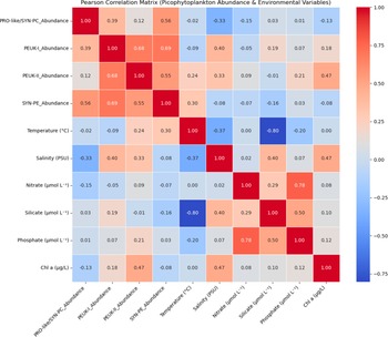
Pearson correlation analysis revealed several linear associations among picophytoplankton groups and environmental variables (Figs 4 & S3). Among picophytoplankton, strong positive correlations were observed between PEUK-I and PEUK-II abundances (r = 0.68) and between PEUK-I and SYN-PE (r = 0.69), with other group pairs showing moderate positive correlations. Among environmental variables, temperature and silicate were strongly negatively correlated (r = −0.80), whereas nitrate and phosphate were strongly positively correlated (r = 0.78). In terms of picophytoplankton-environment relationships, PEUK-II abundance correlated moderately with chl a (r = 0.47), and PEUK-I showed a moderate positive correlation with salinity (r = 0.40). PRO-like/SYN-PC abundance exhibited a weak negative correlation with salinity (r = −0.33). Additionally, weak positive correlations were found between temperature and both PEUK-II (r = 0.24) and SYN-PE (r = 0.30) abundances.

Table III. Independent-samples t-test results: year 2018 vs year 2020.

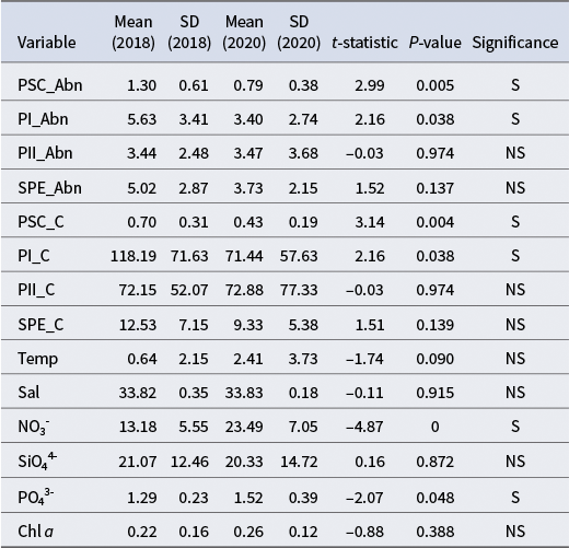
SD = standard deviation; PSC = Prochlorococcus-like/Synechococcus (PRO-like/SYN-PC); PI = PEUK-I; PII = PEUK-III; SPE = Synechococcus with phycoerythrin (SYN-PE); Abn = abundance (cells × 10⁷ l⁻¹); C = carbon (pg C cell⁻¹); Temp = temperature (°C); Sal = salinity (PSU); NO₃^- = nitrate (μmol l⁻¹); SiO₄^4- = silicate (μmol l⁻¹); PO₄^3- = phosphate (μmol l⁻¹); Chl a = chlorophyll a (μg l⁻¹); NS = not significant; S = significant (P < 0.05).

Principal component analysis

PCA was conducted on five key environmental variables - temperature (°C), salinity (PSU), nitrate (μmol l⁻¹), phosphate (μmol l⁻¹) and silicate (μmol l⁻¹) - to identify dominant environmental gradients influencing the study region. The first three principal components (PC1, PC2 and PC3) collectively explained 93.5% of the total variance in the environmental dataset, with individual contributions of 49.1%, 30.2% and 14.2%, respectively.

PC1 was primarily defined by strong positive loadings from silicate (0.575) and phosphate (0.475), along with a negative loading from temperature (−0.460). This axis represents a gradient from warmer, low-nutrient waters to colder, high-nutrient waters. PC2 was characterized by strong negative loadings from nitrate (−0.601), phosphate (−0.480) and Temperature (−0.446), capturing a gradient from warmer, nutrient-rich waters to colder, nutrient-poor conditions. PC3 was dominated by a strong negative loading from salinity (−0.857), delineating a salinity-driven gradient from lower- to higher-salinity waters.

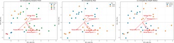
Biplots of sample scores along the principal component axes (Fig. 5a–c) revealed distinct clustering patterns. Samples grouped by oceanic fronts (Fig. 5a) showed clear separation, particularly distinguishing the Antarctic zone/southern Antarctic zone from the STF/subtropical zone along PC1. Similarly, samples from the 2018 and 2020 expeditions (Fig. 5b) were well-separated along PC1 and PC2, indicating pronounced inter-annual environmental variability. In contrast, samples grouped by depth category (DCM vs surface) did not exhibit distinct separation in the PCA space (Fig. 5c), suggesting that vertical differences were less influential in shaping the overall environmental variance structure.

Principal component regression

PCR was conducted using the first three environmental principal components (PC1, PC2 and PC3) as predictors to address multicollinearity.

For Model 1: PEUK-II abundance, the PCR model was statistically significant overall (F-statistic = 3.415, P = 0.0290), explaining 24.2% of the variance (R ² = 0.242, adjusted R ² = 0.171). Among predictors, only PC3 was statistically significant (coefficient = −1.724 × 10⁷, P = 0.004), suggesting that PEUK-II abundance decreases as PC3 increases (i.e. it is higher in lower-salinity waters). PC1 (coefficient = 1.429 × 10⁶, P = 0.637) and PC2 (coefficient = −2.600 × 10⁶, P = 0.501) were not significant (Table S2).

Figure 4. Pearson correlation matrix heatmap showing the linear relationships between picophytoplankton abundance groups and environmental variables (temperature, salinity, nitrate, silicate, phosphate and chlorophyll a (chl a)). PEUK = picoeukaryote; PRO-like/SYN-PC = Prochlorococcus-like/Synechococcus; SYN-PE = Synechococcus with phycoerythrin.

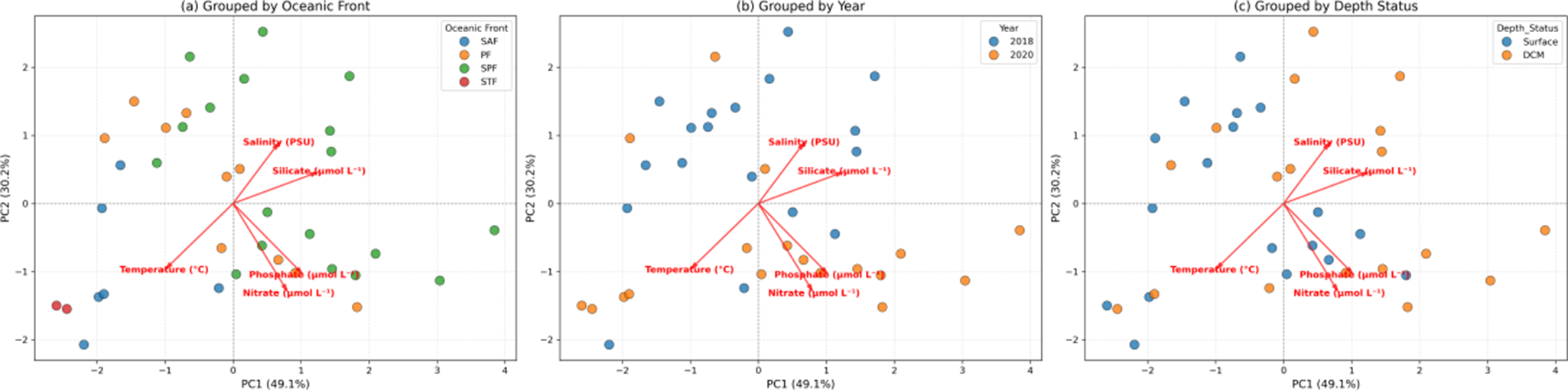
Figure 5. Principal component analysis (PCA) biplots showing the distribution of samples in the PC space, grouped by a. oceanic front, b. year and c. depth status. Environmental variables (temperature, salinity, nitrate, silicate and phosphate) are represented by red vectors indicating their loadings on PC1 and PC2. DCM = deep chlorophyll maximum; PF = Polar Front; SAF = Sub-Antarctic Front; SPF = south of the Polar Front; STF = Subtropical Front.

For Model 2: PRO-like/SYN-PC abundance, the overall model was not statistically significant (F-statistic = 2.068, P = 0.124), explaining a low proportion of variance (R ² = 0.162, adjusted R ² = 0.084). However, PC3 emerged as a significant predictor (coefficient = 2.612 × 10⁶, P = 0.021), indicating that PRO-like/SYN-PC abundance increases with increasing PC3 (i.e. higher in lower-salinity waters). PC1 (coefficient = −2.894 × 10⁵, P = 0.619) and PC2 (coefficient = −1.252 × 10⁵, P = 0.866) were not statistically significant (Table S3).

Discussion

Our findings contribute to a deeper understanding of the ecological niches of distinct picophytoplankton groups in this dynamic, high-latitude system, directly addressing our hypothesis that while PEUK-II abundance would be significantly influenced by major environmental gradients, PRO-like/SYN-PC abundance would not be.

Ecological drivers of picophytoplankton abundance

PCR analysis revealed distinct environmental controls for the two major picophytoplankton groups investigated. As hypothesized, PEUK-II abundance was significantly driven by the primary environmental gradients (PC1, PC2 and PC3), which collectively represent the complex interplay of temperature, salinity, nitrate, phosphate and silicate concentrations. The significant relationships with these principal components suggest that PEUK-II is responsive to multiple, orthogonal environmental axes.

Specifically, based on the new PCA loadings, PC1 (explaining 49.1% of the variance) was primarily characterized by strong positive loadings from silicate (0.575) and phosphate (0.475) and a negative loading from temperature (−0.460). This component represents a gradient from warmer, lower-nutrient (silicate, phosphate) waters to colder, higher-nutrient waters. The non-significant association of PEUK-II with PC1 suggests that it does not singularly drive PEUK-II abundance.

PC2 (explaining 30.2% of the variance) showed strong negative loadings from nitrate (−0.601) and phosphate (−0.480) and a negative loading from temperature (−0.446). This component defines a gradient from warmer, higher-nutrient (nitrate, phosphate) waters to colder, lower-nutrient waters. The non-significant association of PEUK-II with PC2 indicates that this gradient is also not a sole linear driver.

PC3 (explaining 14.2% of the variance) was strongly characterized by a negative loading from salinity (−0.857). The significant negative association with PC3 (P = 0.004) indicates that PEUK-II abundance decreases as PC3 increases, meaning PEUK-II is higher in lower-salinity waters. This suggests that salinity - or factors closely correlated with it - plays a significant role in structuring PEUK-II populations in this region. This could be indicative of freshwater influence from ice melt or specific water masses.

The overall statistically significant PCR model for PEUK-II abundance (R ² = 0.242, P = 0.0290) confirms that while individual PCs may not all be significant, the combined environmental gradients do explain a notable portion of its variability. This reinforces PEUK-II’s sensitivity to dynamic oceanographic conditions. Their higher abundance at DCM depths further supports their adaptation to the moderate light and enhanced nutrient availability often found at the DCM (Boyd et al. 2024, Marañón et al. 2024).

In contrast to PEUK-II, our PCR analysis demonstrated that the abundance of PRO-like/SYN-PC was not statistically significant overall in the PCR model (R ² = 0.162, P = 0.124), but PC3 (salinity gradient) was a significant positive predictor, indicating higher abundance in lower-salinity waters. This crucial finding refutes a universal linear control by these major environmental factors for all picophytoplankton groups. This lack of a strong linear relationship suggests that PRO-like/SYN-PC might be influenced by other, unmeasured environmental factors, such as micronutrients (e.g. iron), specific light regimes or grazing pressure, which were not directly included in this regression model (Hirose et al. 2008, Cunningham & John 2017, Landry et al. 2024). Additionally, non-linear relationships or thresholds might play a role, where their response to environmental change might not be linear, or they might have broad tolerances to these general gradients, only responding to more extreme conditions. Their adaptation to specific oligotrophic niches, particularly for Prochlorococcus-like populations, which are known to thrive in highly oligotrophic conditions (Partensky et al. 1999, Read et al. 2017, Cai et al. 2024), suggests that the variance in these conditions along the transect might not be sufficient for a strong linear driver to emerge. The observed significant inter-annual differences (higher in 2018 vs 2020), despite no strong linear environmental drivers in the PCR, further suggest that larger-scale, perhaps multi-year oceanic variability or unmeasured factors might play a more dominant role in their long-term distribution. Similar depth-related patterns in the picoeukaryotic community assembly have been noted in other oceanic regions (Chen et al. 2023), suggesting that the environmental structuring of these communities is a widespread phenomenon, although the drivers differ by latitude.

Spatial and temporal variability in relation to oceanic features

The observed significant differences in picophytoplankton communities across oceanic fronts and between years highlight the dynamic nature of the Southern Ocean. The clear separation of samples by oceanic fronts and years in the PCA biplots (Fig. 5) corroborates the distinct environmental conditions found in these different water masses and between expeditions. The higher abundances of PEUK-II and SYN-PE at the SAF compared to the PF underscore the role of frontal systems as zones of enhanced biological activity, probably due to nutrient upwelling or specific water mass mixing (Rubin et al. 1998, Bender et al. 2016, Pinkerton et al. 2021, Hörstmann et al. 2021). The significant inter-annual variations for PEUK-I and PRO-like/SYN-PC (higher in 2018) emphasize the importance of long-term monitoring to capture the full range of variability driven by larger climatic oscillations or specific events not apparent in single-year snapshots (Rousseaux & Gregg 2014, George et al. 2022, Giddy et al. 2023). Other studies have similarly shown that picophytoplankton respond dynamically to physicochemical variability, particularly shifts in salinity and nutrient availability (Wei et al. 2019), reinforcing the view that these communities are sensitive indicators of changing oceanographic conditions.

Correlations and environmental linkages

The correlation analysis provided supplementary insights into inter-variable relationships. The strong negative correlation between temperature and silicate and the positive correlation between nitrate and phosphate are consistent with well-established oceanographic patterns globally and within the Southern Ocean, reflecting nutrient remineralization and uptake processes in different water masses (Sarmiento & Orr 1991, Trujillo & Thurman 2017). The moderate positive correlation between PEUK-II and chl a supports the finding that PEUK-II contributes significantly to overall chlorophyll biomass, particularly in more productive environments.

Limitations and future directions

While this study provides robust insights, certain limitations should be acknowledged. Environmental parameters directly incorporated into the multivariate regression model focused on temperature, salinity, nitrate, phosphate and silicate. Other factors such as light availability, mixed-layer depth, iron concentrations (a known limiting nutrient in the Southern Ocean) or grazing pressure were also not directly incorporated. The grouping of PRO-like/SYN-PC due to flow cytometric overlap at these high latitudes, while necessary for the analysis, might obscure distinct ecological responses within these two picocyanobacterial genera. Future research should aim for higher-resolution sampling, both spatially and temporally (e.g. diel cycles, seasonal cruises), to capture finer-scale variability. Additionally, inclusion of additional environmental factors, such as trace metals (especially iron), irradiance and grazer abundance, is needed to build more comprehensive models. Molecular approaches are also recommended to resolve phylogenetic distinctions within picocyanobacteria (e.g. Prochlorococcus clades, Synechococcus clades) and picoeukaryotes, which may exhibit more specific environmental niches. Finally, experimental studies are crucial to validating observed relationships and investigating ecophysiological responses under controlled conditions.

Conclusion

This study provides novel insights into the environmental factors structuring picophytoplankton communities in the Indian sector of the Southern Ocean during austral summers. Our analysis, particularly the robust PCR, confirms our hypothesis by demonstrating distinct environmental controls for different picophytoplankton groups.

We found that the abundance of PEUK-II picophytoplankton is significantly driven by environmental gradients, with PC3 (primarily reflecting a salinity gradient) being a significant predictor. This suggests that PEUK-II abundance is higher in lower-salinity waters, highlighting its sensitivity to specific oceanographic conditions. The overall statistically significant PCR model (R ² = 0.242, P = 0.0290) indicates that the combined environmental gradients (temperature, salinity, nitrate, phosphate and silicate) explain a notable portion of PEUK-II variability.

Conversely, the abundance of PRO-like/SYN-PC picophytoplankton was not statistically significant overall in the PCR model (R ² = 0.162, P = 0.124), although PC3 was again a significant positive predictor. This suggests that while large-scale environmental gradients may not universally drive this group, salinity appears to play a role, and other, unmeasured factors, non-linear responses or more subtle ecological interactions may also govern their distribution in this high-latitude environment.

Furthermore, the study revealed significant spatial variability tied to distinct oceanic fronts and notable inter-annual differences between 2018 and 2020, emphasizing the highly dynamic nature of this ecosystem. These findings collectively underscore the distinct ecological strategies and environmental niches occupied by different picophytoplankton groups, which are crucial for understanding the functioning and resilience of the Southern Ocean’s microbial food web in the face of ongoing environmental change.