


Introduction
The proposal of intelligent manufacturing “2025” has led to the rapid development of industrial automation technology, and it has appeared in the production and manufacturing of enterprises on a large scale. Manufacturing technology is gradually developing in the direction of intelligence, unmanned, and networking, and humans and machines exchange data through interactive systems. The development of intelligent manufacturing technology not only includes technological innovation in intelligent technology and intelligent systems, but also has the function of self-learning, which can be said to be an important direction for the future development of the modern manufacturing industry (Min, Reference Min2018). Printed circuit board PCBs are based on electronic chemicals and are known as the “mother of electronics.” In the electronic information industry, PCB plays an important role, which is widely used in integrated circuits, artificial intelligence, medical equipment, aerospace and industrial equipment, and other fields (Hongyan, Reference Hongyan2022). By connecting circuits, PCBs enable electronic devices to achieve higher performance and provide a better user experience.
Printed circuit board (PCB) manufacturing is developing rapidly as one of the basic and active industries in the electronics industry, and how to manufacture high-quality printed circuit boards in the daily industrial production process is a huge challenge for the industry (Xianyong et al., Reference Xianyong, Junhui, Yuan, Mingsheng, Jinjin and Lin2023). In the production process of PCB, due to the complexity of the production process, each process may lead to defects on the surface of the PCB, such as open circuits, short circuits, residual copper, and leaks. These defects can have a significant impact on the performance, safety, and quality of the final electronic product. Therefore, how to intelligently detect PCB defects has become the focus of attention in the actual production process of the industry. Inconspicuous defects on printed circuit boards can also cause tens of thousands of huge losses, so the defect detection of finished printed circuit boards before leaving the factory is an indispensable quality inspection task.
Traditional printed circuit board inspection is mainly based on the use of specific inspection instruments by workers to determine whether there are defects with the help of visual observation and personal experience. However, this method is not satisfactory in terms of accuracy and efficiency. Then, the industry uses its conductivity to determine whether there is a defect by connecting the printed circuit board to the detector, but due to the instability of the electrical energy generated by the detector, too strong electrical energy may damage the tiny components in the printed circuit board, causing unnecessary economic losses. With the maturity of deep learning technology, related technologies have been selectively introduced to meet the needs of efficient, non-destructive and low-cost industrial production for printed circuit board defect detection tasks (Wu et al., Reference Wu, Zhao, Yuan and Yang2022).
The traditional defect detection method based on image processing achieves acceptable detection accuracy. However, they are time-consuming and sensitive to environmental and inferred images. With the development of deep learning (DL) and computer vision, deep learning and convolutional neural network (CNN) technology have been widely used in PCB defect detection. The existing deep learning object detection methods are mainly divided into single-stage detection algorithms and two-stage detection algorithms. A single-stage algorithm performs a single processing of the entire input image to detect the object. These algorithms typically use a single CNN to perform zone recommendations and object detection. The two-stage algorithm separates object proposal from object detection. The first stage of the two-stage algorithm uses a separate algorithm or network to generate a region proposal; The second stage then performs target detection in these proposed areas. The two-stage detection algorithm is represented by R-CNN (region with CNN characteristics) (Girshick et al., Reference Girshick, Donahue, Darrell and Malik2014), Fast R-CNN (fast region-based CNN) (Girshick, Reference Girshick2015), and Faster R-CNN (Ren et al., Reference Ren, He, Girshick and Sun2017). These algorithms are used to generate candidate boxes and then classify each candidate box. The single-stage detection algorithm consists of the YOLO (You Only Look Once) (Redmon et al., Reference Redmon, Divvala, Girshick and Farhadi2016; Redmon and Farhadi, Reference Redmon and Farhadi2017, Reference Redmon and Farhadi2018; Bochkovskiy et al., Reference Bochkovskiy, Wang and Liao2020) series and the SSD (Single Shot MultiBox Detector) (Liu et al., Reference Liu, Anguelov, Erhan, Szegedy, Reed, Fu and Berg2016). These algorithms directly generate the class probability and position coordinate values of the target while creating candidate frames, and the final detection results can be obtained directly after a single detection. In order to solve the problem that image uncertainty will limit the PCB inspection performance under uneven ambient light or unstable transmission channels, Yu et al. (Reference Yu, Han-Xiong and Yang2023). Designed a new collaborative learning classification model. Zhang et al. (Reference Zhang, Jiang and Li2021). used a cost-sensitive residual convolutional neural network to detect PCB appearance defects, and obtained good detection results. However, the model has a high complexity and a large number of parameters. Based on the Semi-Supervised Learning (SSL) method, Wan et al. (Reference Wan, Gao, Li and Gao2022). used a small number of labeled samples to detect PCB surface defects, which improved the detection efficiency and achieved an average detection accuracy (mAP) of 98.4%. Ding et al. (Reference Ding, Dai, Li and Liu2019). proposed TDD-net (Minor Defect Detection) based on Faster R-CNN for the detection of tiny target defects in PCBs. The accuracy is high, but the model size is too large to be used on embedded devices. Xuan et al. (Reference Xuan, Jian-She, Bo-Jie, Zong-Shan, Hong-Wei and Jie2022) proposed a PCB defect detection algorithm based on YOLOX and coordinate concern, which has good robustness. However, the size of the algorithmic model is 379 MB. Wu et al. (Reference Wu, Zhang and Zhou2022) proposed GSC YOLOv5, a deep learning detection method that integrates lightweight network and dual attention mechanism, which effectively solves the problem of small object detection. However, the proposed attention mechanism is complex and slow. Zheng et al. (Reference Zheng, Sun, Zhou, Tian and Qiang2022) realized real-time detection of surface defects on PCBs based on MobileNet-V2. The mAP of the four types of defects is only 92.86%, which needs to be further improved. Yu et al. (Reference Yu, Wu, Wei, Ding and Luo2022) proposed the Diagonal Feature Pyramid (DFP) to improve the performance of small defect detection. However, the model size is 69.3 MB, which still needs to be further quantified. Other scholars have also proposed a series of detection methods based on deep learning technology, which have the problems of large model size and poor real-time performance.
Therefore, a series of methods based on deep learning do have certain help for the defect detection accuracy of PCB boards in the industry, but there will still be some defects. The method proposed in this paper can effectively extract and fuse information at different scales by adding an attention mechanism and some feature fusion modules. By assigning different attention weights, the model can appropriately weight features at different scales, thereby improving the performance of small target defect detection.
Yolov8 network structure
The YOLO algorithm has developed from v1 to today’s v10, and has gone through some processes, constantly updated and improved, and has an important position in the field of object detection, and continues to develop and improve. It excels in applications that require real-time performance, while also improving accuracy and adaptability. It has a series of advantages such as fast speed, easy deployment, and strong practicability. This paper uses YOLOv8, which is the culmination of the YOLOv8 series of algorithms, which builds on the success of the previous YOLOv5 version, and introduces some innovations and improvements to improve the performance of the model. Specific improvements include the following three aspects: (1) creating a new backbone network; (2) the new Ancher-Free detection head; (3) take advantage of the new loss function. The backbone network refers to the ELAN design idea of YOLOv7 (Wang et al., Reference Wang, Bochkovskiy and Liao2023), and replaces the C3 structure of YOLOv5 with a richer gradient flow. The C2F structure adjusts the number of channels according to different models, which greatly improves the performance of the model. Compared with YOLOv5, the head part has been greatly changed, using the current mainstream decoupling head structure, separating the classification and detection head, and replacing the Anchor-Based with Anchor-Free. The Distribution Focal Loss function is introduced using Task Aligned Assigner’s dynamic positive sample allocation strategy.
Some training techniques were used to further improve the accuracy of the model, such as Mosiac data augmentation (Wang et al., Reference Wang, Bochkovskiy and Liao2021) in terms of data augmentation for training, but borrowing from the training techniques in YOLOX (Ge et al., Reference Zheng, Songtao, Feng, Zeming and Jian2021) and turning off Mosiac augmentation in the last 10 iterations. Strong operation can effectively improve accuracy. Based on the above improvements, the accuracy of the YOLOv8 algorithm is much higher than that of YOLOv5, and it is a new SOTA model. According to the scaling coefficient of the network, five models with different scales are provided: N/S/M/L/X This is shown in Figure 1.

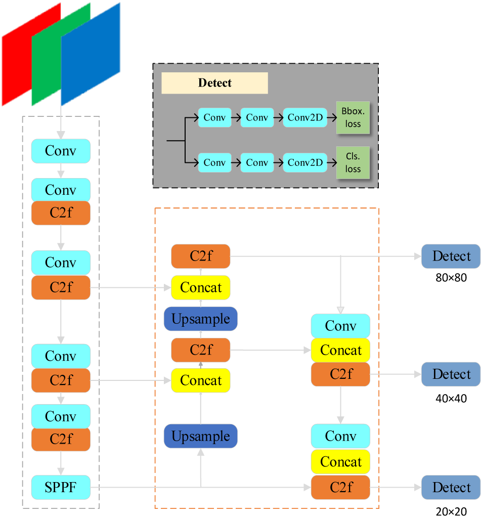
Figure 1. Block diagram of YOLOv8 structure.
In terms of overall design, YOLOv8 includes four parts: data input, backbone, neck, and head (detect). The image data is fed through the input terminal and converted to the format required by the model through Mosiac data augmentation and data preprocessing. Backbone is the backbone network of the object detection model, which is mainly responsible for feature extraction of images. Neck is a link between the backbone and the head, and its main function is to perform feature fusion and processing to improve the detection accuracy and efficiency of the object detection model. The last head part is the last layer of the model, which is mainly responsible for outputting the detection category and location information of the target in the object detection task.
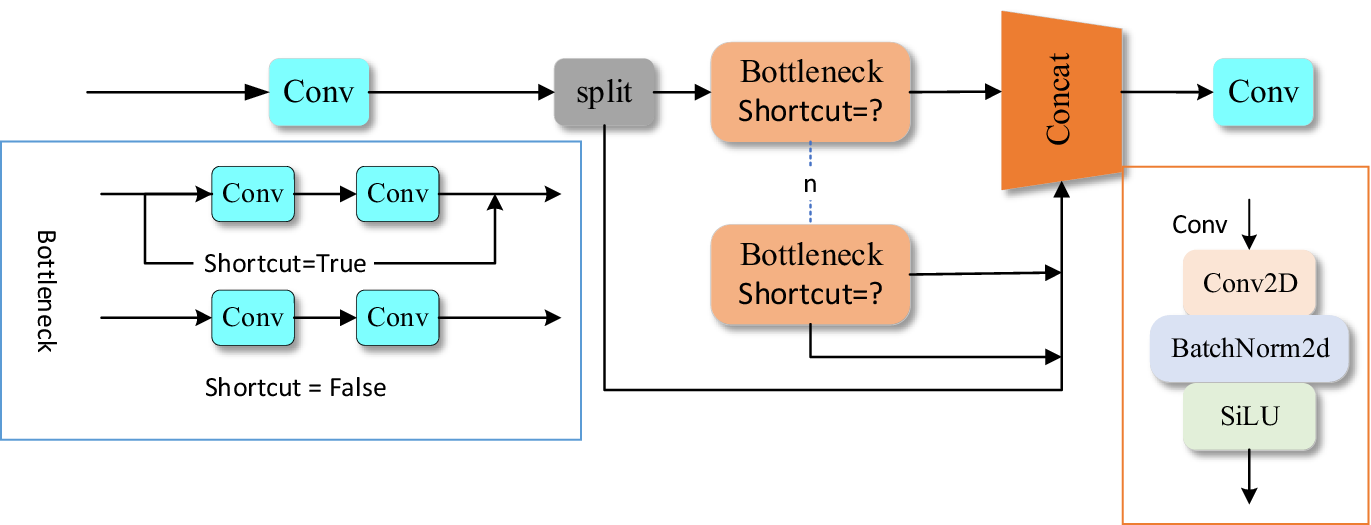
C2f is designed based on the C3 module in YOLOv5, which aims to ensure that the model is lightweight, and at the same time provides richer gradient flow information and reduce the loss of feature information. Moreover, it introduces the idea of efficient lightweight attention network (ELAN) to enhance the performance of the module. It consists of two convolutions, Conv and n*Bottleneck, as shown in Figure 2. Among them, Bottleneck uses the idea of residual network structure, which can better retain the feature details.

Figure 2. C2f module structure diagram.
Improved YOLO algorithm model
GTADH lightweight detection head
In contrast to traditional anchor-based detection methods, YOLOv8 employs an anchor-free detection head design, streamlining the model structure, reducing computational complexity, and potentially enhancing detection accuracy for targets of varying sizes and shapes. Unlike YOLOv5, YOLOv8 separates the predictions for bounding boxes and categories, with each layer featuring two prediction branches: One Hot for category and IOU predictions, and Label and XYWH for bounding boxes. The Task-Aligned Assigner matching method is implemented instead of conventional IOU matching or unilateral proportional allocation, facilitating more accurate assignment of positive and negative labels to training samples, thereby enhancing training efficiency. However, this decoupled architecture, comprising separate branches for classification and box regression, increases model parameters and computational load. To address this, we propose the Group Normalization Task Align Dynamic Detection Head (GTADH), which significantly reduces parameter count through shared convolutional layers (Conv_GN), resulting in a lighter model suitable for resource-constrained devices. Additionally, a Scale layer is incorporated to adjust feature scales across detection heads, further optimizing performance.
As shown in Figure 3, the input feature map is first extracted through two residual connection layers composed of convolution and normalization (Conv_GN) to obtain interactive features. Subsequently, the feature maps are integrated by means of a CONCAT. Since the existing object detector head often uses separate classification and localization branches, this leads to a lack of interaction between the two tasks. Inspired by the idea of Task-aligned One-stage Object Detection (TOOD; Feng et al., Reference Chengjian, Yujie, Yu, Matthew R. and Weilin2021), this paper designs a task alignment structure on the detection head.

Figure 3. Structural diagram of GTADH detection head module.
Through the Task Decomposition Module, the joint features are learned from the interactive features. Then, the localization branch is formed by the deformable convolution (DCNV2) and the offset and mask generated in the interactive features. Similarly, the taxonomic branch is dynamically selected through interactive features. The improved object detection head learns features of different scales by sharing convolution, and then performs classification and localization tasks, so that the two tasks are no longer independent, but select different features through interaction. This not only reduces the number of parameters and calculations of the module, but also significantly improves the detection performance of the detection head.
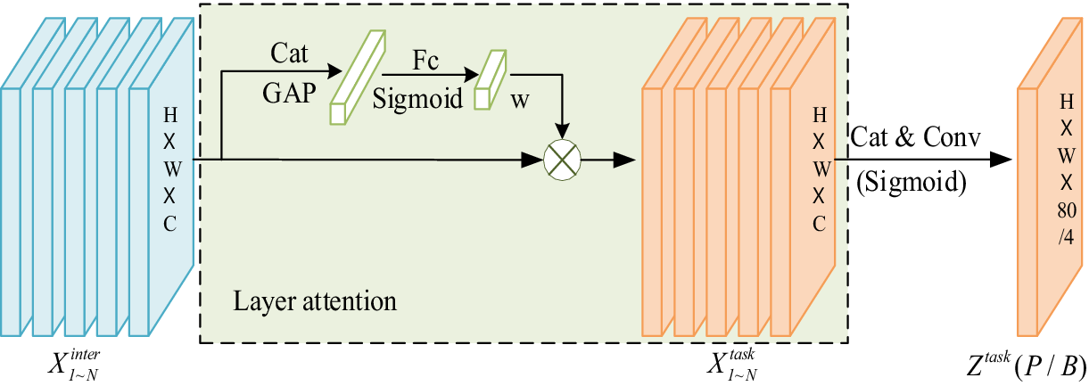
Among them, the structure diagram of the task decomposition module is shown in Figure 4, which proposes a layer attention mechanism to realize task decomposition by dynamically calculating the specific features of different tasks at the level. For classification and localization tasks, their specific characteristics are calculated separately:
 $$ {X}_k^{task}={\omega}_k\ast {X}_k^{\mathit{\operatorname{int}} er},\forall k\in \left\{1,2,\dots ..,N\right\} $$
where ωk is the kth element of the learned layer attention weight ω∈RN. The weight ω is calculated based on the interaction characteristics of the cross-layer task, which captures the interaction between layers
 $$ \omega =\sigma \left( fc2\left( fc1\left({x}^{\mathit{\operatorname{int}} er}\right)\right)\right) $$

Figure 4. Structure of task decomposition module.
fc1 and fc2 are the two fully connected layers. σ is the sigmoid activation function, xinter is obtained by applying average pooling to Xinter, and Xinter is applied to Xkinter Perform the concatenate to get. Finally, the prediction results for classification and positioning are calculated based on the Xtask for each task as follows:
 $$ {Z}^{task}= conv2\left(\delta \left( conv1\left({X}^{task}\right)\right)\right) $$
where Xtask is obtained by Xktask by concatenate. conv1 is a 1x1 convolution operation for dimensionality reduction. Ztask is transformed by the sigmoid activation function to obtain a classification score of P∈RH × W × 80. Then, through the distance-to-bbox transformation, the positioning prediction B∈RH × W × 4 is obtained.
Improved multi-scale feature fusion network structure (FFPN)
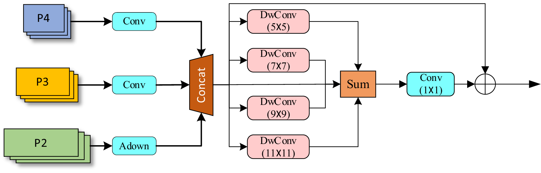
Small targets are easy to be lost with the increase of network depth, feature confusion, semantic information conflict, and weak semantic information correlation between different scales, and the fused features cannot enrich feature information, which is not conducive to small target detection. To solve this problem, this paper proposes an adaptive feature-focused focusing depthwise convolutional module (FDM) module, as shown in Figure 5.

Figure 5. Structure diagram of the adaptive feature-focused FDM module.
Firstly, three feature maps of different scales (P2, P3, and P4) were received, and each feature map was extracted through a convolutional layer. Then, the extracted features are stitched together (Concat). Next, the spliced feature map undergoes four Depthwise Convolutions with different convolution kernel sizes to further obtain feature details. The outputs of these convolutions are superimposed, processed through a 1 × 1 convolutional layer, and finally the results are output by residual connection. The module can focus and fuse features of different scales well to reduce the loss of small target information.
Building on this, the PAN–FPN structure in the neck of YOLOv8 is adjusted to improve feature fusion. Feature pyramid network (FPN) is a framework that combines top-down and bottom-up feature transfer, allowing high-level semantic features to propagate downward, enhancing the overall feature pyramid. However, FPN primarily enhances semantic information, with limited transmission of localization features. To address this limitation, the path aggregation network (PAN) introduces a bottom-up pyramid structure to FPN. PAN employs a path aggregation approach that merges shallow and deep feature maps, enabling the upward transmission of strong localization features from lower levels. This mechanism enhances multi-scale feature representation. The integration of PAN–FPN between the backbone and head components improves performance in both object detection and classification tasks by balancing semantic and localization information more effectively.
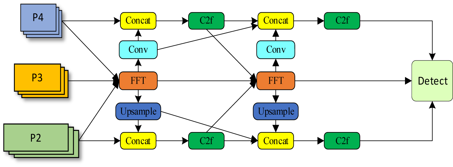
On this basis, this paper proposes a feature-focused pyramid structure (FFPN), an improved multi-scale feature-fused clustering network structure, as shown in Figure 6.

Figure 6. Multi-scale feature fusion aggregation network structure FFPN.
As shown in Figure 6 of the structure above, this part receives feature maps from different levels (P2, P3, P4) and processes them through upsampling, stitching, convolution, and focusing depthwise convolutional module (FDM). Specifically, P2 is stitched with the upsampled P3 feature map and further processed by the C2f layer. After P2, P3, and P4 are processed by FDM, some of them are upsampled and spliced with P2, and the other part is transferred to the next FDM through convolution. After convolution, P4 is stitched with the processed P3 feature map, and then processed by the C2F layer, and finally all the feature maps are transferred to the detection head (Detect). The defect target in the PCB board is small, and this design enhances the network’s ability to detect objects at different scales and resolutions through multi-scale feature fusion, so it is not easy to ignore the feature details for small targets.
Improve the backbone structure of the backbone network
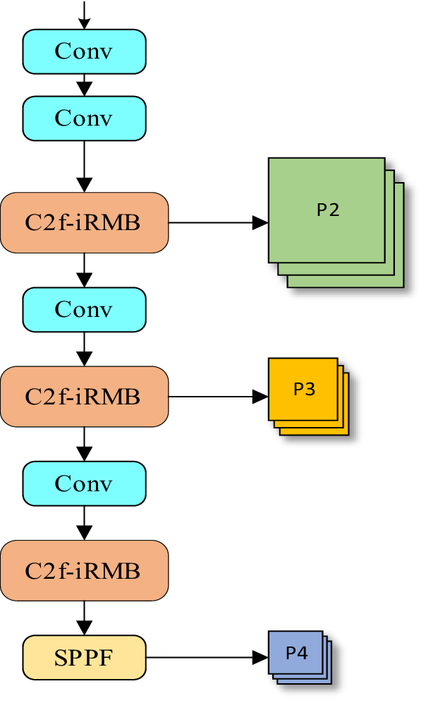
Backbone is an important part of the neural network model, which is mainly responsible for the extraction of target feature information. Due to the small size of the defect target in the PCB board, it is difficult to extract the details of the target image, and the improved backbone and feature extraction module C2f-iRMB are proposed here, as shown in Figures 7 and 8.

Figure 7. Improving the backbone network.

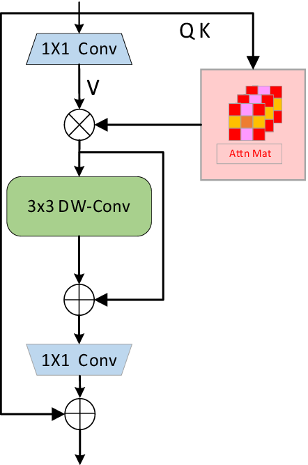
Figure 8. iRMB module structure.
Figure 8 shows the structure diagram of the inverted residual block (iRMB), which combines the dynamic modeling capabilities of the inverted residual block (IRB) and transformer components to create an efficient neural network module. By integrating a variety of techniques in modern deep learning, such as batch normalization, deep convolution, SE attention mechanism and multi-head self-attention mechanism, iRMB realizes the efficient extraction and fusion of feature information.
First, iRMB applies batch normalization to the input data to reduce the internal covariate shift, thereby improving the training speed and stability. The activation function adopts the default Rectified Linear Unit (ReLU) and introduces nonlinearity to enable the model to represent more complex functions. Deep convolution significantly reduces the number of parameters and computations by convoluting each input channel individually. Subsequently, the iRMB module introduces the SE attention mechanism to enhance the feature representation ability of the model by adaptively adjusting the weight of each channel. In the specific implementation process, the SE module is applied after deep convolution to improve the attention to important features. Although the self-attention mechanism can effectively capture the global context information, its computational complexity is high, so iRMB adopts the multi-head self-attention mechanism to divide the input features into multiple heads, and each head independently performs attention calculation, to improve the computational efficiency and feature expression ability.
In the implementation process, the Query, Key and Value matrices are first calculated, and then the attention-weighted sum is performed to obtain the attention output. The input feature map undergoes 1x1 convolution for channel expansion, and then the attention mechanism is enabled. The output of the attention mechanism undergoes 3x3 deep convolution, and finally 1x1 convolution for channel compression to match the channel dimension of the output. Residual joining is an effective method to alleviate the problem of vanishing gradients, which is widely used in deep networks. The iRMB module determines whether to apply a residual connection by judging whether the shape of the input and output is consistent, thus ensuring the stability of the training process. Finally, the feature dimension is adjusted to the desired number of output channels by projection convolution, and regularization is performed using Dropout to prevent overfitting.
Figure 7 shows the improved backbone network structure, because the PCB board detects small defect targets, and the details of small targets will be lost due to the excessive number of convolution layers, so the last layer of the backbone feature extraction network is removed, and the feature details of the detected targets are better retained while reducing the number of parameters. At the same time, the feature extraction layer C2f is replaced by the C2f-iRMB module, which can effectively improve the detection accuracy in feature extraction. The combination of C2f and iRMB modules realizes the efficient extraction and fusion of feature information, and improves the overall expression ability and computational efficiency of the model.
Experimental design
Experimental environment
The experiment in this paper is used to train the model on a server of linux system, the deep learning framework PyTorch version number is 2.0.0, and the programming language Python version number is 3.8 (ubuntu20.04). Cuda version 11.8, NVIDIA GeForce RTX 4090D, 24GB of memory. The processor model is a 15 vCPU Intel(R) Xeon(R) Platinum 8474C. The model training period epochs is set to 600 rounds. Each batch batch size is set to 16; The image input size is 640 × 640; The learning rate (lr0 and lrf) is set to 0.01, the momentum parameter is set to 0.937, and the data load is set to 8. Optimization is carried out using the SGD optimizer.
Datasets
The dataset used in this experiment is the PCB defect dataset published by the Open Laboratory of Human-Machine Switching of Peking University. The dataset contains missing_hole, mouse_bite, open_circuit, short, spur, spurious_ There are six categories of copper, a total of 693 images. Because the target defects of the original dataset are relatively small, the image background is relatively simple, and the dataset has few samples, the model cannot be trained well. In order to have enough. of samples to train the model; and the ability to simulate real-life scenarios; The dataset is enriched by adjusting brightness, occlusion, increasing noise, rotating, cropping, panning, and mirroring the sample through data augmentation. The following figure shows the original image after data enhancement.
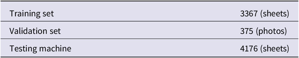
As shown in Figure 9, six different defects are enhanced in different ways, which enriches the diversity of defect sample pictures, and when some of these defects are smaller, the target is more difficult to capture after noise and flip cropping, so it is also more difficult for the experiment. After data augmentation, the dataset is expanded to 4158, and this paper divides the training set (train) and test set (test) according to the ratio of 9:1. The training set (train) and the validation set (test) are divided according to the ratio of 9:1. As shown in the Table 1.

Figure 9. A part of the pictures of each category.
Table 1. Partition of experimental datasets

Evaluation indicators
For the algorithm of the object detection task, the usability of the model and the reliability of the experimental results are evaluated. Detection accuracy, positioning accuracy, and model detection speed are usually used as reference indicators for model performance. In terms of detection accuracy, there are the following parameters: precision and recall, such as Equations (4) and (5); represents the proportion of positives that were correctly predicted and the proportion of positives that were correctly detected in the actual positives, respectively. To assess the balance of the two, the F1-Score is often used.
 $$ P=\frac{\mathrm{TP}}{\mathrm{TP}+\mathrm{FP}} $$
 $$ R=\frac{\mathrm{TP}}{\mathrm{TP}+\mathrm{FN}} $$
where True Positive (TP) denotes a target that was correctly detected; False Positive (FP) denotes the case of being incorrectly detected as a target; and False Negative (FN) denotes a target that was not detected.
In addition, Average Precision (AP) is the area under the curve of accuracy and recall calculated at different thresholds, as shown in Equation (6), and Mean Average Precision (mAP) is averaged for each class of APs in a multi-class detection, as shown in Equation (7), where N is the number of target object categories and i is the AP value of the ith category, It is one of the most commonly used evaluation criteria for object detection.
 $$ \mathrm{AP}={\int}_0^1P(R)d(R) $$
 $$ \mathrm{mAP}=\frac{1}{N}{\sum}_0^N\mathrm{A}{\mathrm{P}}_i $$
In terms of positioning accuracy, Intersection over Union (IoU) is widely used to evaluate the coincidence of the predicted bounding box with the true bounding box, and the higher the IoU value, the more accurate the positioning. The results of object detection are usually set with a certain IoU threshold, such as 0.5 or 0.75, to determine whether the detection is valid. Speed metrics include frames per second (FPS), which measures how fast a model can process in a video stream, and inference time, which represents the time it takes to process a single image, which is important for real-time applications.
In addition, the complexity of the model is often measured by the number of parameters, which reflects the size and complexity of the model, and FLOPs, which represent the amount of computation required to process a single image, with the smaller the FLOPs, the more efficient the model. The performance of the object detection algorithm can be comprehensively evaluated by combining these indicators, and the above parameters are used to evaluate the performance of the model algorithm.
Ablation experiment
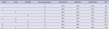
In order to verify the feasibility of the module proposed in this paper, a set of ablation experiments were carried out on the basis of the original dataset, which was the open P CB plate dataset used in the Peking University experiment. In this paper, we combine the improved module with YOLOv8s for comparative experiments, as shown in Table 2, where √ adds the module.
Table 2. Comparison of ablation experimental results

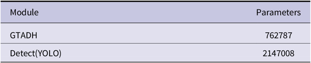
As shown in Table 2, the above ablation experiments show that the accuracy of each module has been improved. The original mAP value was increased from 96.4% to 98.5%, and the overall detection accuracy was improved by 2.1%. In particular, the GTADH module contributes the most to the improvement of model accuracy, because this detection head extracts and shares the detection target data, so that the information between detection and classification can be exchanged. This has been experimentally proven to be feasible, and the number of parameters has also been reduced compared to the original detection head, as shown in Table 3.
Table 3. Comparison of GTADH and Detect

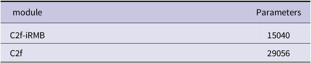
As shown in the table above, the GTADH head has nearly 60% less parameters than the original one, further illustrating the Conv_GN caused by these two devices. The benefits of the normalized residual extraction feature sharing can further simplify the model parameters compared with the original three sets of convolutions extracting features separately. In addition, the Reverse Residual Moving Block (iRMB) is added to C2f, which is a feature extraction module combined with the attention mechanism, which enhances the selectivity of the model for features and focuses on specific features or information compared with the traditional attention mechanism. The experiment in Table 2 also has an improvement effect, and it does not increase the number of parameters of the model, this paper also does a comparative experiment, as shown in Table 4, after the introduction of this module, the overall parameter quantity of the C2f module decreases by about 50%, without affecting the accuracy improvement, the number of parameters of the model is reduced. Figure 10 shows the specific AP value improvement of the improved model on various datasets.
Table 4. Comparison of C2f and C2f- iRMB


Figure 10. Comparison of AP values of each category of the improved model with the previous model.
Through the above pictures, it can be intuitively seen that the improved model has improved the AP value of each category, which once again proves the feasibility of the experiment in this paper, and the proposed improved module has an improvement in the accuracy of each category. The improvement is particularly obvious for defects such as “spur,” and the accuracy AP value has increased from 91.9% to 96.3%, an increase of 5.6 percentage points. It can be seen that the model in this paper makes a great contribution to the improvement of the accuracy of such defects.
Comparative experiments
To further validate the proposed model’s performance improvements, the test set described in Section “Datasets” was utilized to assess the model’s generalization capabilities under consistent experimental settings and parameters. Various models, representing current mainstream object detection frameworks, were selected for comparative analysis, including YOLOv8s, YOLOv5s, Faster R-CNN, EAM-YOLOv8s, and YOLOv8 with Swin Transformer. Evaluation metrics, such as Precision, Recall, mAP, and F1 score, were employed to quantify performance. The results of this comparative experiment are presented in Table 5.
Table 5. Comparative tests of the models

Among the comparisons of these models, the improved YOLO proposed in this paper is the best choice due to its excellent performance. It achieves 99.2% Precision, 96.8% Recall, 98.5% mAP50, and 81.2% at the more stringent mAP50:90, demonstrating its accuracy and comprehensiveness in detecting small targets. At the same time, its model size is only 8.9 MB, which is much smaller than other models, which makes it highly useful even in resource-constrained environments. In addition, an F1 score of 0.98 further demonstrates the model’s good balance between accuracy and recall.
In contrast, YOLOv8s and EAM-YOLOv8s also have high Precision (98.4% and 98.5%, respectively) and Recall (94.8% and 92.9%), but mAP50:90 is slightly less impressive, at 73.9% and 69.9%, respectively. Although YOLOv8-swintransformer is close on mAP50 and Recall, it has a large model size (66.7 Mb) and may not be suitable for scenarios with strict requirements for computing resources. In comparison, the traditional Faster RCNN has lower performance, with less than 85% of both Precision and Recall, and the large model size (108 Mb) makes it less efficient and performant than the YOLO series models.
After comparing the improved model with other mainstream detection algorithms, the loss function, precision, and recall rate (loss) of Improved YOLO and the original YOLOv8s training process are shown in Figures 11 and 12 Recall) and mAP. As shown in Figure 11, the accuracy, recall, and changes in MAP50 and MAP50:95 with training rounds are shown, and each graph measures the performance of the model with the number of training cycles as the horizontal axis.

Figure 11. Comparison of the metric curves of the improved model and the original model.

Figure 12. Comparison of the loss curves of the improved model and the original model.
As you can see that with the increase of training rounds, precision: As you can see from the upper left corner of the chart, the improved YOLO performs slightly better in terms of accuracy, especially in the early stage of training, which converges faster and remains stable when approaching the value of 1.0; Recall: In the recall curve in the upper right corner, the recall rate of the improved version of YOLO is also higher than that of YOLOv8s, indicating that the model has better performance in detecting more real positive samples. mAP 0.5: The lower left corner shows the average accuracy (mAP) of the two models at a threshold of 0.5. The improved version of YOLO showed a higher mAP of close to 1.0, indicating that it was able to effectively detect targets at lower thresholds. mAP 0.5:0.95: The curve in the lower right corner is the most stringent measure of average precision (mAP 0.5:0.95), which considers multiple thresholds from 0.5 to 0.95. The improved version of YOLO consistently outperforms YOLOv8s, especially in the later stages, showing better convergence and achieving higher mAP values.
In Figure 12, the loss curve of the improved YOLO and YOLOv8s over 600 training cycles is shown. Overall, the improved YOLO shows a faster downward trend in both the box loss and the CLS loss on the training and validation sets, and converges to lower values in the later stage. This shows that the improved version of YOLO is better optimized for targeting and classification tasks, especially in terms of border regression. On the classification task, the loss curves of the two models tend to be consistent, but the classification loss of YOLOv8s is slightly higher in the initial stage.
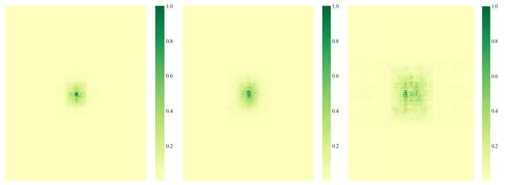
Therefore, for the detection of small targets on PCB boards, the improved model is better than the original model in terms of accuracy index and loss index. The results show that the improved model is slightly better than the original model in terms of small target detection performance. In addition, the receptive field is particularly important for the improvement of small target detection. To further verify the model, the trained model was taken and 50 images were taken based on the test set and input into the network model, and the receptive field visualization schematic diagram was obtained in the feature extraction part of the model and Neck, as shown in Figures 13 and 14, respectively, and the improved model was compared with the model proposed in this paper.

Figure 13. Rendering of the improved receptive field of the model.

Figure 14. Renderings of the receptive field of the model before improvement.
As can be seen from Figures 13 and 14, in the pre-improved receptive field map, we can see that the response in the center of the feature map is stronger, but the response in the edge region is weaker. This indicates that the model mainly focuses on the local area of the image, especially the central position, and ignores the peripheral part of the image in the process of feature extraction. The previous model may have difficulty capturing the global information in the image due to the small receptive field, resulting in insufficient understanding of the larger target or global context. The central region responds obviously, which means that the model mainly relies on the information of the smaller region, which can easily lead to the overfitting of the model to small targets or poor performance in complex scenarios.
In the improved receptive field map, the feature response is not only strong in the central region, but also clearer in the periphery. This indicates that the receptive field is expanded and the model can extract features over a large area, not just in the local area. Through the feature extraction of the attention mechanism module, the receptive field of the model pays more attention to small target detection. In the process of feature extraction, the model no longer relies only on local information but can capture more global features. As can be seen from the visualization of the Neck part, the improved model responds more evenly to different scales, which helps to improve the performance of the model in multi-scale object detection. Although the improved model showed a large receptive field in the last layer, the capture of small targets was not fully optimized overall. Small object detection requires the model to pay attention to local details while avoiding ignoring these small targets due to a large receptive field. Through this improvement, the detection ability of the model for small targets has been enhanced, especially in the feature extraction and Neck parts. By reasonably expanding the receptive field, it ensures that the model can capture the detailed information of small-scale targets more accurately while paying attention to the overall information, to improve the detection accuracy.
To further evaluate the performance of the model, some test set pictures were selected to use the two models for heat map visualization, and the same picture was selected to see the heat map display effect, as shown in Figure 15. A heatmap is a visualization tool that shows the intensity distribution of 2D data, and through the variation of color shades, the heatmap helps us quickly understand how much attention the model is focusing on the target. In feature visualization of neural networks, hotspot areas often indicate that the model has a high level of interest in that region. In contrast to hot spots, cold spots (low-intensity areas) indicate low data values for certain areas that the model or system does not pay much attention to.

Figure 15. Comparison of heat maps before and after the improved model.
Comparing the performance of the two models “Improve YOLO” and “YOLOv8s” in Figure 15 on different defect categories (e.g., missing_hole, mouse_bite, open_circuit, short, spur, spurious_copper), from the visual effect of each defect category, “Improve YOLO” shows more accurate localization ability in detecting certain small targets or small defects. Especially in the detection of subtle defects such as mouse_bite and spurious_copper, the annotation is clearer; While YOLOv8s can detect these defects, some details may be slightly blurry, suggesting that the sensitivity to small targets may not be as strong as the improved model. “Improve YOLO” seems to have better coverage and annotation of defects distributed at multiple points across the board, and multiple defects can be accurately marked. Although the inspection results of “YOLOv8s” can also mark most defects, in some cases, some smaller, more distant defects are not fully labeled; For each defect category, “Improve YOLO” shows a more consistent detection effect in most categories, and can stably capture all kinds of defects; On the other hand, “YOLOv8s” is slightly less effective at detecting certain defect categories (such as spur and spurious_copper) and may have missed some smaller defects. The detection results of “Improve YOLO” show that the model may be more adaptable to different types of defects, especially the detection of small targets is more obvious, and is suitable for precision detection tasks.
Conclusions
Considering the challenge of detecting small targets on PCB boards, real-time defect detection in factory settings is crucial. This paper proposes several improvements based on YOLOv8, introducing three key modules: the Group Normalization Task Align Dynamic Detection Head (GTADH), a feature fusion structure (FFPN), and the integration of a reverse residual moving block (iRMB) within the C2f module, along with an enhanced backbone structure. Through ablation and comparative experiments, results demonstrate that the improved modules reduce model parameters and enhance performance. Specifically, compared to the original YOLOv8s, the model’s detection performance improves by 1.3% on mAP@0.5, reaching 98.5%. Additionally, the more stringent detection metric, mAP@0.5:0.9, shows a 7.3% increase, while the model size is reduced by 60%, making it more suitable for lightweight deployment. In comparison with other mainstream algorithms, the improved model achieves better accuracy and recall, significantly reducing false positives and missed detections. Future work will focus on further optimizing the model to enhance detection accuracy and robustness, aiming to address a wider range of small-target defect detection scenarios.


 Open access