


1. Introduction
The timing of home-leaving has been found to be an important determinant of many life-course outcomes, being associated with partnership formation and fertility patterns (Aparicio-Fenoll and Oppedisano (Reference Aparicio-Fenoll and Oppedisano2015)), internal migration rates (Becker et al. (Reference Becker2010)), income growth (Billari and Tabellini (Reference Billari and Tabellini2011), Kaplan (Reference Kaplan2012)), intergenerational exchange (Rosenzweig and Wolpin (Reference Rosenzweig and Wolpin1993), Leopold (Reference Leopold2012)), and the well-being of parents and children (Mazzuco (Reference Mazzuco2006), Mitchell and Lovegreen (Reference Mitchell and Lovegreen2009), Mencarini et al. (Reference Mencarini2017)).
While many economic and demographic determinants of home-leaving have been extensively studied, less attention has been devoted to the role of cultural factors in shaping the transition to independent living. In this paper, we contribute to this literature by studying how the timing of home-leaving by parents affects that of children by combining data on the life-course decisions of successive generations of European families. We theoretically discuss how a positive intergenerational correlation in home-leaving ages can result from multiple channels, and we exploit a rich set of information to disentangle the role played by the inheritance of status from the transmission of values and preferences concerning the appropriate timing of the exit from the parental home. Our results suggest that most of the intergenerational correlations reflect the cultural transmission channel.
We exploit data from the Survey of Health, Ageing, and Retirement in Europe (SHARE), featuring detailed information on the life-course trajectories of 260,000 individuals born between 1907 and 2001. We are able to link parents and their adult children from around 40,000 households across 20 European countries and to observe the home-leaving patterns of both generations, in addition to detailed life histories for the parents. We focus on home-leaving decisions for two main reasons. First, home-leaving is often considered the first major step in the transition to adulthood. Since all subsequent life-course transitions are influenced by this initial move, it serves as a key vantage point from which to examine the intergenerational transmission of broader patterns in the timing of the transition to adulthood. Additionally, for the adult children we only observe the timing of home-leaving, as SHARE does not contain information on their age at first marriage or childbearing. We are therefore not able to estimate intergenerational correlations for the timing of these other life events. We estimate survival models that naturally account for both right- and left-censored observations, finding that a 1-year increase in the home-leaving age of a parent delays the nest-leaving decisions of her children by approximately one month. From a gender perspective, we find that the effect is slightly larger for sons. Geographically, we illustrate larger effects for Southern, Central, and Eastern European countries with respect to Northern and Western ones. Leveraging detailed information on the socio-economic background of parents, as well as their educational and occupational trajectories and life-course events, we are able to shed light on the relative strength of competing transmission mechanisms. By netting out confounding due to persistence in socio-economic background and education, as well as the direct influence of parental nest-leaving on future incomes, we show that the effect is mainly driven by direct cultural transmission.
We support this claim by performing a heterogeneity analysis that produces two key results. First, the effect of maternal home-leaving ages is twice as large as that of paternal ones, consistently with cultural transmission being driven by the parent children spent the most time with (childcare was mainly a maternal responsibility in the generations we study, as many women were not part of the labor force). Second, the effect is almost four times larger for children whose parents left home for reasons related to family formation (the birth of a child or the start of a marriage or cohabitation spell), consistently with the cultural transmission of preferences for home-leaving being stronger when associated with a major life-course event within the family sphere. We stress, though, that our results hold even in those families in which parents left home for reasons not related to family formation (e.g., pursuing an higher education). This shows that home-leaving per se impacts life-course choices of children, even if it’s not connected to family formation decisions. This further indicates that studying the transmission of home-leaving choices on top of that of other life course events is valuable on its own. We also run a set of robustness checks that establish that our results hold even under different specifications for the empirical model, as well as for relevant subsamples of our data. Overall, our results provide strong evidence for the existence of a strong, direct cultural transmission of preferences regarding the appropriate timing of exit from the parental home.
2. Related literature
In recent years, the transition to independent living has been postponed across many countries, (Mazurik, Knudson, and Tanaka (Reference Mazurik, Knudson and Tanaka2020), Esteve and Reher (Reference Esteve and Reher2021)): this led to the birth of a vast empirical literature studying the drivers of (as well as the obstacles to) youth emancipation. A strand of this literature has focused on constraints hampering home-leaving, including job insecurity (García-Ferreira and Villanueva (Reference García-Ferreira and Villanueva2007), Fernandes et al. (Reference Fernandes2008), Becker et al. (Reference Becker2010), Kaplan (Reference Kaplan2012)), low incomes (Aassve, Billari, and Ongaro (Reference Aassve, Billari and Ongaro2001)), and high house prices (Modena and Rondinelli (Reference Modena and Rondinelli2012), Cooper and Liu (Reference Cooper and Liu2019)). Other studies investigated how home-leaving patterns were influenced by demographic trends, including the changes in the structure of the family of origin, such as the fall in family size (De Falco, Moracci, and Venturin (Reference De Falco, Moracci and Venturin2024)) and the diffusion of non-intact families (Mitchell, Wister, and Burch (Reference Mitchell, Wister and Burch1989)). A smaller literature has instead explored the role played by cultural changes in delaying the home-leaving decisions of young adults. Giuliano (Reference Giuliano2007) exploited second-generation European immigrants in the US as a way to elicit the role of different cultures keeping local economic conditions fixed, finding that cultural background proxied by family origin had sizeable effects on the timing of home-leaving, and claiming that the sexual revolution of the 1970s increased the North-South gap in intergenerational coresidence by liberalizing attitudes of Southern European parents. The importance of culture in shaping home-leaving decisions has been confirmed by many other studies. Zorlu and Mulder (Reference Zorlu and Mulder2011), studying differences in home-leaving patterns between migrant and native youths in the Netherlands, confirm that different cultural backgrounds are source of heterogeneity in behavior. Similar findings are obtain by Lei and South (Reference Lei and South2016), who claim that a large portion of racial and ethnic gaps in home-leaving patterns in the US are explained by cultural differences.
This study analyzes the role played by a specific component of cultural background: the timing of nest-leaving decisions by parents. Several existing studies suggest that previous generations’ decisions on their own exit from the parental home might shape the transition to adulthood of successive generations. For instance, Aassve, Arpino, and Billari (Reference Aassve, Arpino and Billari2013) document sizeable variation across European countries in perceived age norms regarding the appropriate timing of exit from the parental home and find a positive association with actual choices. If parents adhere to norms regarding the appropriate age to achieve independence and transmit them to their children, one should expect to observe intergenerational persistence in home-leaving patterns across successive generations. Positive intergenerational correlations have already been found in the timing of many life-course events, including divorce, fertility, and cohabitation (Wolfinger (Reference Wolfinger2000), Murphy and Knudsen (Reference Murphy and Knudsen2002), Smock, Manning, and Dorius (Reference Smock, Manning and Dorius2013)). This paper investigates whether a similar degree of persistence can be found in the timing of home-leaving.
3. Theoretical framework
The main goal of this paper is to estimate intergenerational correlations in home-leaving ages by linking parents’ and children’s life course trajectories. Intergenerational correlations might stem both from the transmission of values and that of opportunities (Keijer, Liefbroer, and Nagel, Reference Keijer, Liefbroer and Nagel2018). In this Section, we argue that persistence in home-leaving behavior across generations can emerge as a by-product of (i) confounding due to the intergenerational transmission of socio-economic status, (ii) indirect transmission through resources, and (iii) direct cultural transmissionFootnote 1 . We also discuss how we use data from the SHARE survey to disentangle each channel. Figure 1 summarizes our framework using a simple path diagram.

Figure 1. Theoretical framework.
3.1. Confounding: the transmission of socio-economic status and education
Parental resources could be a major determinant of the decision to leave home, even though it is theoretically ambiguous whether having wealthier parents should accelerate or postpone home-leaving. As hypothesized in Avery, Goldscheider, and Speare (Reference Avery, Goldscheider and Speare1992), wealthier parents might be able to provide location-specific luxuries that increase the value of intergenerational co-residence and thereby postpone home-leaving. Angelini, Bertoni, and Weber (Reference Angelini, Bertoni and Weber2022) show that individuals that grow up in a “golden nest” (a family with high socioeconomic status) leave home later. Similar results are obtained by Manacorda and Moretti (Reference Manacorda and Moretti2006), who show that an increase in parental income induces children to leave the parental home later. On the other hand, Avery, Goldscheider, and Speare (Reference Avery, Goldscheider and Speare1992) also notice that, as parental income increases, economies of scale that can be achieved through co-residence become less relevant; moreover, wealthy parents have the resources to help their children to become independent. In principle, depending on whether parents value co-residence with children more than privacy or vice versa, the effect of parental income could have either sign. Other findings in the literature support this hypothesisFootnote 2 .
Enrollment in higher education and educational attainment influence youth independence and nest-leaving patterns as well. Again, however, different studies find effects of opposite signs. Chiuri and Del Boca (Reference Chiuri and Del Boca2010) find that having a tertiary education degree is associated with higher likelihood of cohabiting with parents. Schwanitz, Mulder, and Toulemon (Reference Schwanitz, Mulder and Toulemon2017) show that enrollment in education is associated with a higher risk of leaving the parental home to live without a partner and that after completing education, adults with higher educational attainment are more likely to move out than less educated ones. Angelini, Bertoni, and Weber (Reference Angelini, Bertoni and Weber2022) show that individuals who acquire more education leave the nest at later ages.
Finally, there is a large literature in economics showing that both resourcesFootnote 3 (see Olivetti and Paserman (Reference Olivetti and Paserman2015) and Braun and Stuhler (Reference Braun and Stuhler2018), among others) and educational attainment (Güell, Mora, and Telmer (Reference Güell, Rodríguez Mora and Telmer2015), Colagrossi, d’Hombres, and Schnepf (Reference Colagrossi, d’Hombres and Schnepf2020), Adermon, Lindahl, and Palme (Reference Adermon, Lindahl and Palme2021), Collado, Ortuño-Ortín, and Stuhler (2022)) exhibit a strong degree of persistence through generations. These mechanisms, taken together, would possibly induce a positive intergenerational correlation in the timing of exit which is merely due to confounding. In this paper, we rely on detailed information on the socio-economic status of grandparents and on the educational careers of parents and children in order to explicitly account for these transmission mechanisms in our empirical specification. In particular, we exploit data on the living conditions of parents during childhood in order to control for grandparental resources. We also include the highest educational attainment of parents and the entire educational trajectories of children. Omitting these factors would lead to picking up spurious associations between home-leaving ages driven by these channels, which have been already widely investigated by the literature.
3.2. Indirect transmission through resources
A second portion of the intergenerational correlation between home-leaving ages can be attributable to a combination of two channels: i) home-leaving ages affect the occupational achievement and lifetime resources of parents; ii) parental resources impact their children’s home-leaving patterns (as already mentioned).
There are only a few papers that try to study the consequences of early/delayed home-leaving on later incomes, and the evidence they put forward is inconclusive. Billari and Tabellini (Reference Billari and Tabellini2011) find that Italian youths who leave the parental home later have lower-paying jobs, although it is hard to rule out selection effects (see Pistaferri (Reference Pistaferri2010)). Focusing on the US, Kaplan (Reference Kaplan2012) finds that young adults who have the chance to co-reside with their parents can afford to accept riskier jobs characterized by steeper wage growth profiles, as they can rely on parental support, ultimately obtaining higher life-cycle earnings. These findings suggest that the decision to move out from the parental household might influence labor market trajectories, with a long-term effect on occupational achievement and therefore on parental income. The sign of such effect is however ambiguous, hence we do not have clear expectations on how omitting parental resources from our specification may affect our estimates. We rely on information on the occupational trajectories of parents in order to account for parental resources (which might be affected by parental home-leaving ages) in our empirical models and to measure the contribution of this channel to the overall association.
3.3. Direct cultural transmission
The residual channel is direct cultural transmission. As mentioned in the Introduction, there is plenty of evidence showing that cultural background (Giuliano (Reference Giuliano2007), Zorlu and Mulder (Reference Zorlu and Mulder2011)) is associated with life-course decisions including leaving the parental home. One channel through which cultural background influences these decisions is the presence of culture-specific norms about the appropriate timing and ordering of life-course events (Aassve, Arpino, and Billari (Reference Aassve, Arpino and Billari2013)). As these norms are inherited through socialization, the role of families and especially parents in transmitting them is extremely relevant. Keijer, Liefbroer, and Nagel (Reference Keijer, Liefbroer and Nagel2018) distinguish two mechanisms through which socialization operates. On one hand, previous generations transmit values to successive ones; henceforth, children develop attitudes that are aligned with those of parents. On the other, parents can become models for children: successive generations imitate the behavior of previous ones, irrespective of their set of values. Keijer, Liefbroer, and Nagel (Reference Keijer, Liefbroer and Nagel2018) find that both these channels play a role in generating persistence in life-course decisions. As our data doesn’t enable us to disentangle these two channels, we have to interpret our estimated direct cultural effect as the sum of these two components.
We will interpret the residual association between parental and children’s home-leaving ages after controlling for the two above-mentioned channels as a measure of whether direct cultural transmission exists and to what extent it contributes to the observed unconditional correlation between parental and children home-leaving ages.
4. Empirical analysis
4.1. Data
We exploit data from the Survey of Health, Ageing, and Retirement in Europe (SHARE), a large, cross-national panel survey that started in 2004, covering 27 European countries and Israel. The survey has a total of nine waves; in this study, we exploit data from waves 1–7. It is focused on the elderly population (all respondents are aged 50 or more at their first interview). In regular panel waves, respondents provide information on their current labor market status, health conditions, asset holdings and many more. Moreover, they are asked to provide several details about their children, including their sex, year of birth and, most importantly, whether each child is still co-residing with them. In case a child has left home at the moment of the interview, they report the home-leaving yearFootnote 4 . Moreover, in waves 3 and 7 respondents provide extensive retrospective information about their own life-courses, by answering a life-history questionnaire named “SHARELIFE”. This additional data enables us to observe the educational and labor market trajectories of SHARE respondents, as well as to obtain information on their socio-economic background through a series of questions on their economic conditions during childhood. Crucially, respondents are also asked about their complete residential history, in particular the year in which they left the (grand) parental household in order to start living on their own. This allows us to observe, for each child-parent dyad, the home-leaving ages of both individuals. Leveraging on this unique piece of information, we can study the vertical transmission of home-leaving patterns. Notice that in what follows we sometimes denote SHARE respondents as “parents” or “generation 1” (G1) and their children as “adult children” or “generation 2” (G2).
4.2. Sample restrictions
We only focus on natural adult children, thereby excluding adopted or foster children of SHARE respondents. We drop children that are less than 16 at the moment of the interview, and those adult children that report to have left home before 17 or after 39Footnote 5 . We implement the latter restriction as we want to focus on the transition to independent living of young adults. For a similar reason, we also exclude children whose parents report home-leaving ages smaller than 10 and larger than 40. We exclude families with more than 13 children. Despite SHARE also features data from Israel, we exclude it from our analysis to focus on European countries.
4.3. Descriptive statistics
In Table 1 we display summary statistics on our sample of adult children and on their fathers and mothers. Clearly, not all children mentioned by respondents have both parents participating in the survey. One obvious reason is that, as SHARE is a survey of the elderly, the partners of respondents might have already died when the interview takes place. In our final sample of around 102,000 adult children, we have information on both parents for around 53% of individuals, while we only have information on mothers (fathers) for 33% (13%) of them. The average G2 adult children in our sample is born around 1973, but we have huge variation as the youngest individual is born in 2001 and the oldest is born in 1920. Adult children are on average 40 when their old parents are interviewed. The median number of siblings is two. The average home-leaving age is relatively low (23.2), one of the reasons being that only 87% of adult children have already left the nest when their parents are interviewed. The presence of right censoring tilts the mean to the left of the home-leaving age distribution. Notice that our data also features around 8000 left censored histories (see Figure B.1 in the Appendix), i.e., those for which the parent states that his/her adult child has already left home at the time of the interview, but does not remember when. Most adult children have medium to high educational achievement (measured by ISCED-97 levels). From a geographical perspective, the sample is quite evenly spread across EuropeFootnote 6 . The average parent (G1) in our sample is born around 1945-46 and aged around 66 when interviewed. While we have perfect balance in terms of sex for the children sample, this doesn’t hold for the sample of SHARE respondents, where females are over-represented. Average home-leaving ages are smaller for mothers than for fathers, and so are marriage ages and ages at first childbirth, due to the standard gendered age gap in couples.
Table 1. Summary statistics

Note: Highest educational attainment is classified according to ISCED-97 levels (0–1–2 = low, 3–4 = medium, 5–6 = high). The reason to leave home for G1 is assumed to be family formation when in a one-year span around the leaving-home age the individual started cohabiting, married or became a parent.
As already mentioned, we have remarkable cohort coverage as we are able to observe parent-child dyads spanning around a century: the oldest G1 individual is born in 1908, while the youngest G2 is born in 2001. Figure 2 describes the cohort composition of our sample, distinguishing between birth years of adult children (G2) and their mothers and fathers (G1).
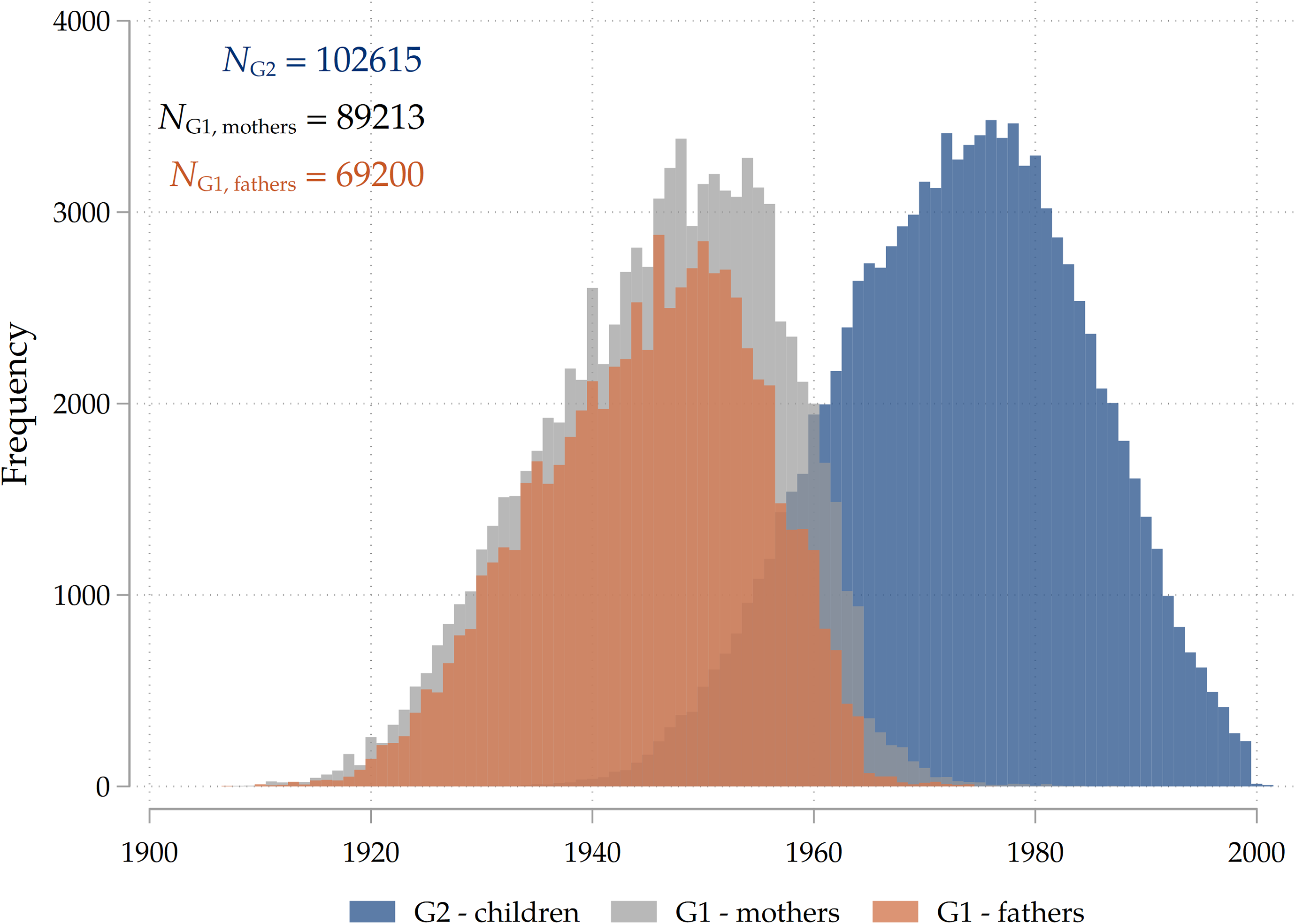
Figure 2. Cohorts covered by SHARE.
Our data enables us to study in detail the home-leaving patterns of two generations of individuals. In Figure 3 we display survival curves for adult children and for their parents. Notice that individuals from G1 leave home before their children, on average: this is a consequence of the increase in rates of intergenerational co-residence over time, with people from more recent cohorts leaving the parental household laterFootnote 7 .

Figure 3. Home-leaving profiles in SHARE.
With SHARE data at hand, it is possible to provide preliminary descriptive evidence on the existence of a raw positive association between parental and children’s home-leaving ages. Figure 4 plots the average emancipation age of children grouped according to the home-leaving age of their parents (we pick the father if there is available information on his home-leaving patterns and the mother if we only have information on her home-leaving ageFootnote 8 ). The graph reveals a clear, strong, positive association between home-leaving ages of successive generations, as expected. On average, in our analytical sample, adult children whose parents left home at 20 years of age leave the parental home when they are 22–23, around 2.5 years before than adult children whose parents left home around 30. The associations with paternal and maternal home-leaving ages look fairly similar. In the next Section, we will present the empirical setting that will allow us to estimate conditional correlations that take into account the set of potential confounders and mediating variables discussed in Section 3.
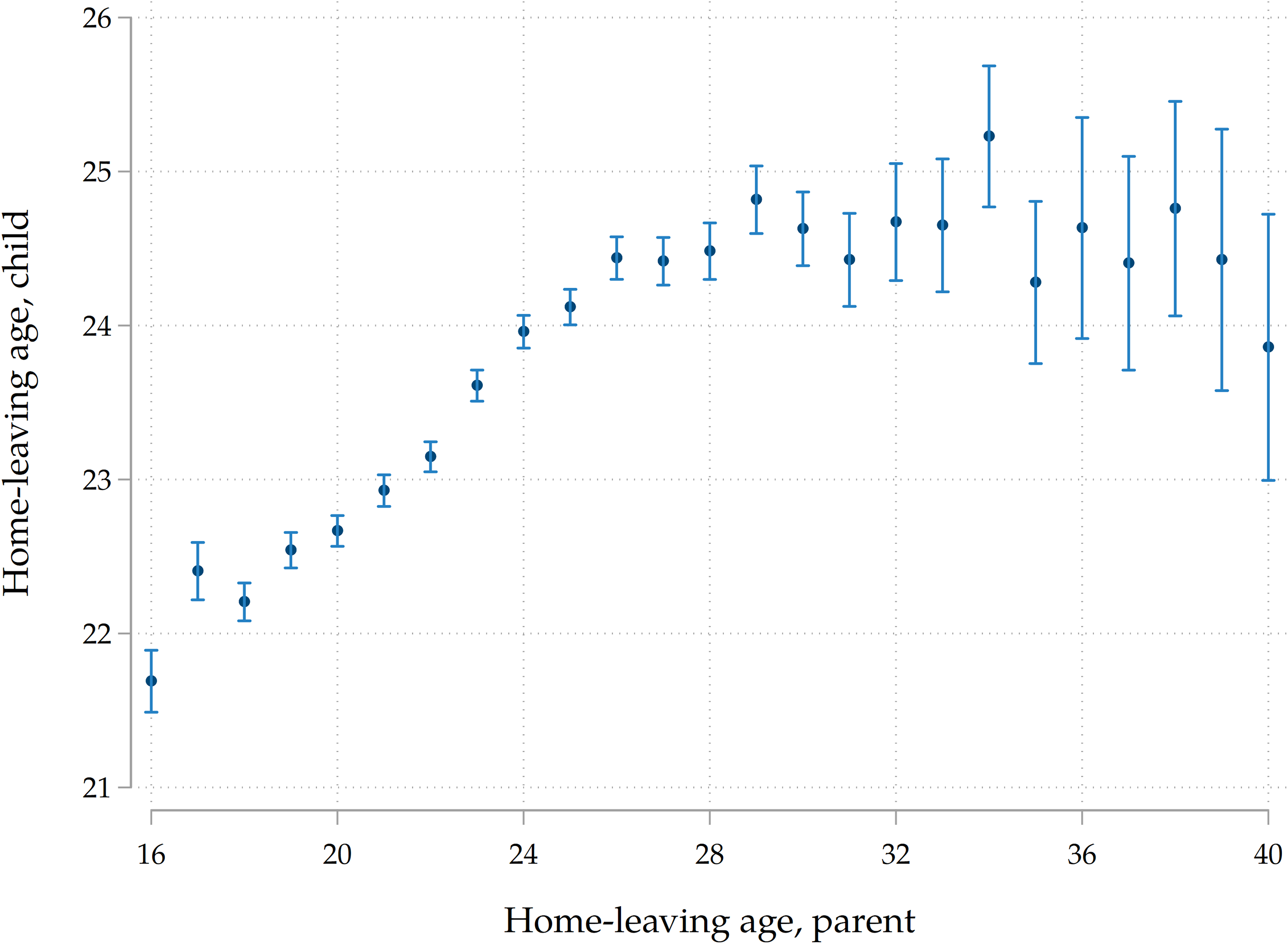
Figure 4. Average home-leaving age of parents and their children.
4.4. Empirical strategy
Let
 $T$
denote home-leaving age and
$T$
denote home-leaving age and
 ${T}_{Par}$
denote parental home-leaving age. Ultimately, we are interested in the association between the home-leaving ages of parents and that of children, i.e., we would like to estimate the derivative
${T}_{Par}$
denote parental home-leaving age. Ultimately, we are interested in the association between the home-leaving ages of parents and that of children, i.e., we would like to estimate the derivative
 ${{\partial T} \over {\partial {T_{Par}}}}$
. We cannot rely on a simple linear regression model as we have to deal with a sizeable amount of left and right censored observations, as highlighted in Figure B.1 in the Appendix. Therefore, we exploit a survival model that takes both into account. Notice that with a standard discrete-time model for the hazard, we would need to exclude left-censored observations. In order to avoid this information loss, we model the survival function instead. As a robustness check, we repeat the analysis excluding left-censored observations and adopting a standard discrete-time model for the hazard.
${{\partial T} \over {\partial {T_{Par}}}}$
. We cannot rely on a simple linear regression model as we have to deal with a sizeable amount of left and right censored observations, as highlighted in Figure B.1 in the Appendix. Therefore, we exploit a survival model that takes both into account. Notice that with a standard discrete-time model for the hazard, we would need to exclude left-censored observations. In order to avoid this information loss, we model the survival function instead. As a robustness check, we repeat the analysis excluding left-censored observations and adopting a standard discrete-time model for the hazard.
Let
 $S\left(a\right)$
denote the survival function, with
$S\left(a\right)$
denote the survival function, with
 $a$
representing age. We use the following notation to stress that the survival function might depend on parental home-leaving ages
$a$
representing age. We use the following notation to stress that the survival function might depend on parental home-leaving ages
 $$S(a,{T_{Par}}) = {\rm{Pr}}\left( {T \gt a|{T_{Par}}} \right).$$
We want to estimate the marginal effect of
 ${T}_{Par}$
on the shape of the survival function, i.e, our estimand of interest is
${T}_{Par}$
on the shape of the survival function, i.e, our estimand of interest is
 ${{\partial S\left( {a|{T_{Par}}} \right)} \over {\partial {T_{Par}}}}$
. In order to estimate it, we have to define the dummy variable
${{\partial S\left( {a|{T_{Par}}} \right)} \over {\partial {T_{Par}}}}$
. In order to estimate it, we have to define the dummy variable
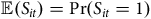
 $${S_{it}} = \left\{ {\matrix{ 1 {\,\,\,\,} {{\rm{if}}} {\,\,\,\,} {Ag{e_{it}} \ge {T_i}} \hfill & {} \hfill \cr 0 {\,\,\,\,} {{\rm{if}}} {\,\,\,\,} {Ag{e_{it}} \lt {T_i}} \hfill & {} \hfill \cr}} \right.$$
which describes the home-leaving trajectories of adult children in our sample. We make the simplifying assumption that leaving-home is a non-reversible process, i.e., we abstract from the possibility of boomeraging. Notice that we have info on
 ${S}_{it}$
even for individuals who are right-censored (for whom
${S}_{it}$
even for individuals who are right-censored (for whom
 ${S}_{it}=1$
for any
${S}_{it}=1$
for any
 $t \lt t_i^{\rm{*}}$
, the interview time) or left-censored (for whom
$t \lt t_i^{\rm{*}}$
, the interview time) or left-censored (for whom
 ${S}_{it}=0$
for any
${S}_{it}=0$
for any
 $t \ge t_i^{\rm{*}}$
). We estimate logit models of the type
$t \ge t_i^{\rm{*}}$
). We estimate logit models of the type
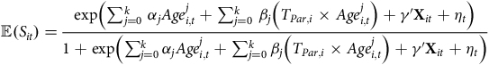 $$\mathbb{E}\left( {{S_{it}}} \right) = {{{\rm{exp}}\left( {\mathop \sum \nolimits_{j = 0}^k \,{\alpha _j}Age_{i,t}^j + \mathop \sum \nolimits_{j = 0}^k \,{\beta _j}\left( {{T_{Par,i}} \times Age_{i,t}^j} \right) + \gamma {\rm{'}}{{\bf{X}}_{it}} + {\eta _t}} \right)} \over {1 + {\rm{exp}}\left( {\mathop \sum \nolimits_{j = 0}^k {\alpha _j}Age_{i,t}^j + \mathop \sum \nolimits_{j = 0}^k {\beta _j}\left( {{T_{Par,i}} \times Age_{i,t}^j} \right) + \gamma {\rm{'}}{{\bf{X}}_{it}} + {\eta _t}} \right)}}$$
where
 ${T}_{Par,i}$
is some measure of parental home-leaving ages for adult children
${T}_{Par,i}$
is some measure of parental home-leaving ages for adult children
 $i$
and
$i$
and
 ${\mathbf{X}}_{it}$
is a set of controls that differ across specificationsFootnote
9
. We run the model for different values of
${\mathbf{X}}_{it}$
is a set of controls that differ across specificationsFootnote
9
. We run the model for different values of
 $k$
to assess the sensitivity of our results to different choices of the polynomial fit. In the Appendix we show that from the estimated marginal effects
$k$
to assess the sensitivity of our results to different choices of the polynomial fit. In the Appendix we show that from the estimated marginal effects
 ${{\partial S\left( {a|{T_{Par}}} \right)} \over {\partial {T_{Par}}}}$
it is possible to obtain an estimate
${{\partial S\left( {a|{T_{Par}}} \right)} \over {\partial {T_{Par}}}}$
it is possible to obtain an estimate
 $\widehat {{{\partial T} \over {\partial {T_{Par}}}}}$
of the marginal effect of parents leaving home one year later on the average home-leaving age of children.
$\widehat {{{\partial T} \over {\partial {T_{Par}}}}}$
of the marginal effect of parents leaving home one year later on the average home-leaving age of children.
4.5. Model specifications
We run three specifications that differ from each other in the set of variables included. In our first specification, X it only includes baseline controls such as sex, country, number of siblings, birth order, birth year, and parental year of birth. In our second specification, X it also includes the time-varying educational achievement of the child, a time-varying student dummy, as well as the highest educational achievement of the parent. It also includes a continuous index for the socio-economic background of the parent’s family of origin (grandparental resources) constructed by exploiting information on his/her living conditions when 10. In order to construct the index, we use the approach proposed by Angelini, Bertoni, and Weber (Reference Angelini, Bertoni and Weber2022) for SHARE data: we perform a polychoric principal component analysis to extract the first component from four proxies of socio-economic status of the grandparental family (occupation of main breadwinner in the household, presence of fixed bath/toilet and other amenities, number of books at home, number of rooms per capita)Footnote 10 . Finally, in our third specification, X it also includes parental occupational achievement which we collapse in two categories (low-tier and high-tier occupations) in order to reduce dimensionality. We define occupational achievement as the occupation held at the end of the working life. As all respondents are aged 50 or above, we assume that even if they are not retired when interviewed, their current position is the last one they will hold. For retired individuals, we use the last reported occupation before retirement. In Table 3, we display the distribution of occupational achievement in our sample of parents, at the ISCO 1-digit aggregation level. From the Table, it is possible to see that the number of parents for which we have information on occupations is smaller than the total number of parents reported in Table 1. In order to keep the analytical sample fixed across specifications, we run all models only on the subsample of individuals that have no missing information on each of the covariates included in our third specification.
The choice of the three specifications described above is driven by the theoretical framework described in Section 3. Our first specification is meant to capture the association between home-leaving ages of successive generations once that we account for basic demographic features of parents and children such as their country of residence, year of birth, as well as the number of siblings and birth order of children, which have been found to be relevant predictors of home-leaving patterns. The estimates derived from this first specification are still subject to an important source of confounding, i.e., the intergenerational transmission of characteristics that affect home-leaving. Our second specification attempts to account for this mechanism by including variables that capture persistence in socio-economic background and educational choices (i.e., the socio-economic background and education of parents, as well as educational trajectories of their children). Our final and third specification also includes the occupational achievement of parents, in the form of a dummy for high-low tier occupation based on the ISCO codes of the last job position. INSERT INFO ON HIGH LOW ISCO. Explicitly including parental occupational achievement is meant to capture a possible channel through which parental home-leaving ages might affect those of their children, beyond direct cultural transmission: namely, the effect of parental home-leaving patterns on children’s home-leaving via the mediating role of parental income.
In order to estimate the model, we have do define an appropriate measure of parental home-leaving ages
 ${T}_{Par,i}$
. In order to maximize the sample size for our main empirical analysis, we construct the following measure that enables us to define parental home-leaving ages for the entire sample of adult children, i.e., we use the variable
${T}_{Par,i}$
. In order to maximize the sample size for our main empirical analysis, we construct the following measure that enables us to define parental home-leaving ages for the entire sample of adult children, i.e., we use the variable
 $${T_{Par,i}} = \left\{ {\matrix{ {{T_{Father,i}}} \hfill & {{\rm{if}}} \hfill & {{T_{Mother,i}} \ne \cdot \wedge {T_{Father,i}} \ne \cdot } \hfill \cr {{T_{Father,i}}} \hfill & {{\rm{if}}} \hfill & {{T_{Mother,i}} = \cdot \wedge {T_{Father,i}} \ne \cdot } \hfill \cr {{T_{Mother,i}}} \hfill & {{\rm{if}}} \hfill & {{T_{Mother,i}} \ne \cdot \wedge {T_{Father,i}} = \cdot } \hfill \cr } } \right.,$$
i.e., we use the home-leaving ages of fathers whenever they are available and those of mothers otherwise. We prioritize information about fathers since they are more likely to report their occupation. Given this choice, we also control for the sex of the selected parent in all our specifications. When we run analyses for the subsample of individuals for whom we have information on both parents’ home-leaving patterns, we either include the average parental home-leaving age
 ${T}_{Par,i}$
or we include both
${T}_{Par,i}$
or we include both
 ${T}_{Father,i}$
and
${T}_{Father,i}$
and
 ${T}_{Mother,i}$
in the specification as separate treatments, in order to disentangle the effect of paternal and maternal home-leaving ages on children’s decisions.
${T}_{Mother,i}$
in the specification as separate treatments, in order to disentangle the effect of paternal and maternal home-leaving ages on children’s decisions.
5. Results
The main set of results is displayed in Figure 5, where we plot the average marginal effects of
 ${T}_{Par}$
on the survival function
${T}_{Par}$
on the survival function
 $S(a,{T}_{Par})$
for our three different specifications.Footnote
11
The plotted lines must be interpreted as the derivative of the survival function with respect to
$S(a,{T}_{Par})$
for our three different specifications.Footnote
11
The plotted lines must be interpreted as the derivative of the survival function with respect to
 ${T}_{Par}$
. The Figure clearly shows that the marginal effect on the survival function is almost always positive, i.e., that staying-home probabilities are positively associated with delayed exit by parents. Notice that the marginal effect of
${T}_{Par}$
. The Figure clearly shows that the marginal effect on the survival function is almost always positive, i.e., that staying-home probabilities are positively associated with delayed exit by parents. Notice that the marginal effect of
 ${T}_{Par}$
on the survival function is hump-shaped: the effect is close to zero around 16 and 40 years of age, where all the members of our analytical sample are respectively still at home or already living independently, while it reaches the maximum size around the average home-leaving ages (23–25 years) of G2.
${T}_{Par}$
on the survival function is hump-shaped: the effect is close to zero around 16 and 40 years of age, where all the members of our analytical sample are respectively still at home or already living independently, while it reaches the maximum size around the average home-leaving ages (23–25 years) of G2.

Figure 5. Results on the entire sample, all specifications.
Note: The Figure displays average marginal effects of a 1-year increase in
 ${T}_{Par}$
on
${T}_{Par}$
on
 $\mathbb{E}\left( {{S_{it}}} \right) = {\rm{Pr}}({S_{it}} = 1)$
, i.e., it plots
$\mathbb{E}\left( {{S_{it}}} \right) = {\rm{Pr}}({S_{it}} = 1)$
, i.e., it plots
 $\widehat{\partial S\left(a\right)/\partial {T}_{Par}}$
(as well as its 95% confidence intervals for each marginal effect) for each value of age
$\widehat{\partial S\left(a\right)/\partial {T}_{Par}}$
(as well as its 95% confidence intervals for each marginal effect) for each value of age
 $a \in \{ {\rm{16}},{\rm{17}}, \ldots, 40\} $
. On top of each panel we display
$a \in \{ {\rm{16}},{\rm{17}}, \ldots, 40\} $
. On top of each panel we display
 $\widehat{\partial T/\partial {T}_{Par}}$
, the estimated effect of a 1-year increase in
$\widehat{\partial T/\partial {T}_{Par}}$
, the estimated effect of a 1-year increase in
 ${T}_{Par}$
on
${T}_{Par}$
on
 $T$, the age at home-leaving of the child. Standard errors are clustered at the family level. Each plot corresponds to one of the three specifications discussed above.
In our baseline model, where we only include basic demographic controls (country of birth, family size, birth order, and birth years for the parent-child dyad), we find that a 1-year increase in
 ${T}_{Par}$
increases survival (home-staying) probabilities for all ages between 20 and 35, and it decreases them (slightly) for ages 16–18 and 36–40. This pattern overall generates a positive effect of a 1–year increase in
${T}_{Par}$
increases survival (home-staying) probabilities for all ages between 20 and 35, and it decreases them (slightly) for ages 16–18 and 36–40. This pattern overall generates a positive effect of a 1–year increase in
 ${T}_{Par}$
on
${T}_{Par}$
on
 $T$
, the expected age at home-leaving of the child, which is delayed by slightly less than a month (26 days). As expected, after controlling for the intergenerational transmission of socio-economic background and education-by including the educational trajectories of each parent-child dyad and our measure of parental socio-economic background-the derivative of the survival function decreases in magnitude, but only to a very limited extent: the delay in exit implied by a 1-year increase in the parental home-leaving age shrinks to 24 days. As the third panel shows, the estimated correlation is virtually unaffected by including parental occupational achievement. Estimated effect sizes, once expressed in terms of standard deviations of the treatment and the outcome, are substantial. A one-standard-deviation increase in parental home-leaving ages (roughly equivalent to a 4-year postponement of exit, see Table 1) is associated with a 4-month increase in home-leaving ages of adult children, which is close to one-tenth of the standard deviation of home-leaving ages of G2.
$T$
, the expected age at home-leaving of the child, which is delayed by slightly less than a month (26 days). As expected, after controlling for the intergenerational transmission of socio-economic background and education-by including the educational trajectories of each parent-child dyad and our measure of parental socio-economic background-the derivative of the survival function decreases in magnitude, but only to a very limited extent: the delay in exit implied by a 1-year increase in the parental home-leaving age shrinks to 24 days. As the third panel shows, the estimated correlation is virtually unaffected by including parental occupational achievement. Estimated effect sizes, once expressed in terms of standard deviations of the treatment and the outcome, are substantial. A one-standard-deviation increase in parental home-leaving ages (roughly equivalent to a 4-year postponement of exit, see Table 1) is associated with a 4-month increase in home-leaving ages of adult children, which is close to one-tenth of the standard deviation of home-leaving ages of G2.
We confirm that the positive association between home-leaving ages of successive generations is still present after conditioning on a large set of explanatory variables, including covariates that proxy for the intergenerational transmission of socio-economic background and educational attainment, which may have induced a spurious correlation between our variables of interest. The inclusion of such information reduced the size of the estimated coefficients, as expected, but did not substantially change the quantitative relevance of the effect. The inclusion of parental occupation, a possible channel through which the home-leaving age of parents impacts that of their children (via their effect on parental income) did not change our results at all. Taken together, these results have three main takeaways. First, there is a positive bias in the raw association between home-leaving ages of successive generations when one omits information on socio-economic background and education, which correlate with home-leaving ages and are vertically transmitted. Second, we found no substantial evidence of an indirect effect of parental home-leaving ages on children’s ones through an impact of exit patterns on future parents’ income. Third, and more importantly, we found evidence of the existence of a strong, direct cultural transmission channel that contributes to the observed correlation to a major extent. In Section 6, we will provide additional results that bolster our interpretation of this residual channel as a cultural transmission mechanism.
Heterogeneity by sex. We run models that feature an interaction effect between parental home-leaving ages by sex of the child to understand if there are any differences in the intergenerational transmission of home-leaving ages across sexes. In Figure 6 we show the results for our third specification, the most complete one. Consistently with the evidence on the entire sample, we find that the marginal effects peak around the average home-leaving age: this happens around 25–26 years of age for men and a bit earlier (around 23–24 years) for women. We find that under our full specification, the association seems stronger for men, by a slight margin: the effect on the expected age at home-leaving is a 26–day delay, against a 22–day delay for women. In Figure 6 in the Appendix, we show the results for all three specifications. We find that the bias induced by intergenerational transmission is much stronger for men than for women (a 3–days difference vs less than a 1–day one in terms of increase in the expected home-leaving age). Including parental occupational achievement slightly negatively affects estimates for both sexes.
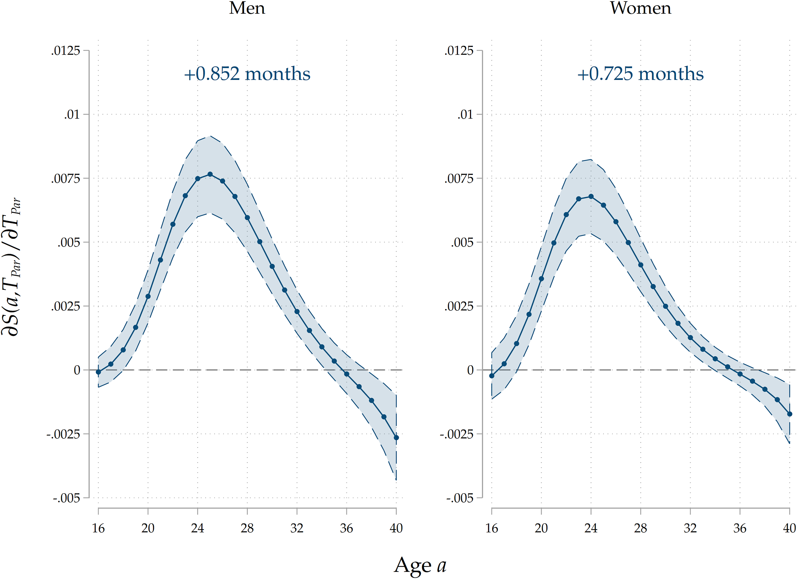
Figure 6. Results by sex of adult child.
Note: The Figure displays average marginal effects of an 1-year increase in
 ${T}_{Par}$
on the survival function
${T}_{Par}$
on the survival function
 $S\left(a\right)$
and on
$S\left(a\right)$
and on
 $T$
, the age at home-leaving of the child, for both sexes of adult children. On top of each panel we display
$T$
, the age at home-leaving of the child, for both sexes of adult children. On top of each panel we display
 $\widehat{\partial T/\partial {T}_{Par}}$
, the estimated effect of a 1-year increase in
$\widehat{\partial T/\partial {T}_{Par}}$
, the estimated effect of a 1-year increase in
 ${T}_{Par}$
on
${T}_{Par}$
on
 $T$
, the age at home-leaving of the child. Standard errors are clustered at the family level. The coefficients reported are for the full specification that includes demographics, socio-economic family background of parents, parental and child education, and parental occupation.
$T$
, the age at home-leaving of the child. Standard errors are clustered at the family level. The coefficients reported are for the full specification that includes demographics, socio-economic family background of parents, parental and child education, and parental occupation.
Heterogeneity by country group. We also run the analyses separately for different country groups. Given that the effects of an increase in parental home-leaving ages is potentially nonlinear (a 1–year increase from 18 to 19 years can have a different impact with respect to an increase from 28 to 29 years), and given that country groups are characterized by very different average ages at home-leaving, in order to make a meaningful comparison we run a model where we include a second-degree polynomial for parental home-leaving ages, and we compute marginal effects of an increase in
 ${T}_{Par}$
at
${T}_{Par}$
at
 ${T}_{Par}=25$
. The results are reported in Figure 7: again, we only report results for our third specification. We find that parental home-leaving ages are significantly positively associated with children’s ones across all the four regions. Notice that, for each curve, the effect is more sizeable around the average home-leaving age of children in each country group: the effect peaks around 20–24 years of age for Northern and Western countries, and around 26–28 for Central/Eastern and Southern countries, reflecting regional differences in the timing of home-leaving. This can be interpreted as evidence that cultural transmission impacts home-leaving decisions for those who leave at ages around the average one, while it has little effect on early leavers and late stayers. The overall effect is stronger for Southern and Eastern countries than for Western, and especially Northern ones. This pattern is consistent with our interpretation of the effect as an estimate of direct cultural transmission: given that family ties are stronger in Mediterranean and Central/Eastern countries than in Western and Northern ones (see Reher (Reference Reher1998), Alesina and Giuliano (Reference Alesina and Giuliano2014)), the fact that the estimated effect is larger in size for the former country groups is consistent with parents’ influence on their children growing with the strength of their ties. In Figures D.12 to D.15 in the Appendix, we show the results for all three specifications for each country group. In Southern countries, a larger portion of the raw intergenerational association is removed after controlling for education and socio-economic background, suggesting a higher degree of persistence. The reduction in the effect is less sizeable in Western and Eastern countries, and it even flips in sign for Northern countries. Across all country groups, including parental occupations has a small, negative effect on the association, suggesting the presence of a small negative effect of leaving home later on occupational trajectories, which mediates the intergenerational relationship.
${T}_{Par}=25$
. The results are reported in Figure 7: again, we only report results for our third specification. We find that parental home-leaving ages are significantly positively associated with children’s ones across all the four regions. Notice that, for each curve, the effect is more sizeable around the average home-leaving age of children in each country group: the effect peaks around 20–24 years of age for Northern and Western countries, and around 26–28 for Central/Eastern and Southern countries, reflecting regional differences in the timing of home-leaving. This can be interpreted as evidence that cultural transmission impacts home-leaving decisions for those who leave at ages around the average one, while it has little effect on early leavers and late stayers. The overall effect is stronger for Southern and Eastern countries than for Western, and especially Northern ones. This pattern is consistent with our interpretation of the effect as an estimate of direct cultural transmission: given that family ties are stronger in Mediterranean and Central/Eastern countries than in Western and Northern ones (see Reher (Reference Reher1998), Alesina and Giuliano (Reference Alesina and Giuliano2014)), the fact that the estimated effect is larger in size for the former country groups is consistent with parents’ influence on their children growing with the strength of their ties. In Figures D.12 to D.15 in the Appendix, we show the results for all three specifications for each country group. In Southern countries, a larger portion of the raw intergenerational association is removed after controlling for education and socio-economic background, suggesting a higher degree of persistence. The reduction in the effect is less sizeable in Western and Eastern countries, and it even flips in sign for Northern countries. Across all country groups, including parental occupations has a small, negative effect on the association, suggesting the presence of a small negative effect of leaving home later on occupational trajectories, which mediates the intergenerational relationship.
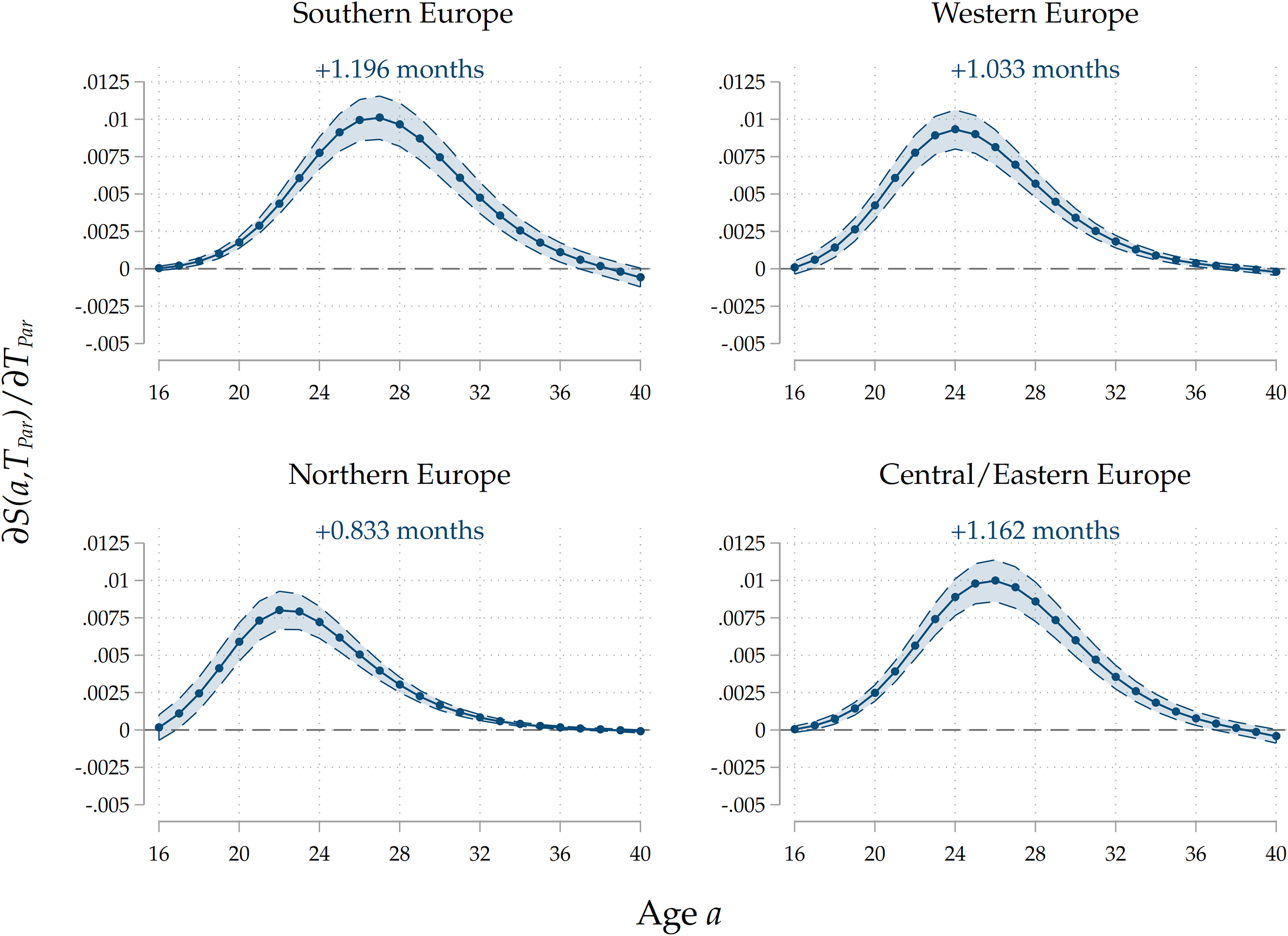
Figure 7. Results by country group.
Note: The Figure displays average marginal effects of an 1-year increase in
 ${T}_{Par}$
on the survival function
${T}_{Par}$
on the survival function
 $S\left(a\right)$
and on
$S\left(a\right)$
and on
 $T$
, the age at home-leaving of the child, for the four groups of countries included in SHARE. The marginal effect of
$T$
, the age at home-leaving of the child, for the four groups of countries included in SHARE. The marginal effect of
 ${T}_{Par}$
is evaluated at
${T}_{Par}$
is evaluated at
 ${T}_{Par}=25$
in order to make comparisons across groups possible. On top of each panel we display
${T}_{Par}=25$
in order to make comparisons across groups possible. On top of each panel we display
 $\widehat{\partial T/\partial {T}_{Par}}$
, the estimated effect of a 1-year increase in
$\widehat{\partial T/\partial {T}_{Par}}$
, the estimated effect of a 1-year increase in
 ${T}_{Par}$
on
${T}_{Par}$
on
 $T$
, the age at home-leaving of the child. Standard errors are clustered at the family level. The coefficients reported are for the full specification that includes demographics, socio-economic family background of parents, parental and child education, and parental occupation.
$T$
, the age at home-leaving of the child. Standard errors are clustered at the family level. The coefficients reported are for the full specification that includes demographics, socio-economic family background of parents, parental and child education, and parental occupation.
6. Additional evidence on direct cultural transmission
Overall, our estimates suggest a pretty high degree of intergenerational transmission of home-leaving patterns. By running several models in which we increasingly augment the set of controls in order to discriminate between different transmission mechanisms, our results are indicative of a strong cultural component in the persistence of home-leaving patterns across generations. In this Section, we provide further evidence that our results are really capturing direct cultural transmission.
Maternal vs paternal home-leaving ages. First, we do so by estimating our baseline model for the subsample on which we have info on both mothers and fathers and by separately including maternal and paternal home-leaving ages. This is indicative about the channel we have in mind, for two reasons. First, given that the majority of parents (G1) in our sample are born around the 1940–1950 period, most families in our analysis are characterized by a male-breadwinner model. This is also consistent with Table 3, which shows that the share of mothers that never had a job is 13 times larger than that of fathers. As highlighted by Keijer, Liefbroer, and Nagel (Reference Keijer, Liefbroer and Nagel2018), this implies that women from these generations spent much more time than men socializing with their children, so that their values and example as role models is possibly more relevant. Second, it has been shown (Sharabi (Reference Sharabi2015)) that mothers have more influence on the family decisions of their children, while father affect more job-related choices. Therefore, we expect the marginal effects of maternal home-leaving ages to be stronger than those of fathers. The estimation results that we show in Figure 8 are clearly consistent with this hypothesis. The marginal effect of a 1-year delay in home-leaving by mothers on a child’s nest-leaving decision is twice as large as that of the same delay in fathers’ choices. We take this as evidence that direct cultural transmission indeed plays a sizeable role.

Figure 8. Separate effects of maternal and paternal home-leaving ages.
Note: The Figure displays average marginal effects of an 1-year increase in
 ${T}_{Father}$
and
${T}_{Father}$
and
 ${T}_{Mother}$
, respectively, on the survival function
${T}_{Mother}$
, respectively, on the survival function
 $S\left(a\right)$
and on
$S\left(a\right)$
and on
 $T$
, the age at home-leaving of the child. On top of the two panels we display
$T$
, the age at home-leaving of the child. On top of the two panels we display
 $\widehat{\partial T/\partial {T}_{Father}}$
and
$\widehat{\partial T/\partial {T}_{Father}}$
and
 $\widehat{\delta T/\delta {T}_{Mother}}$
, respectively the estimated effect of a 1-year increase in maternal and paternal home-leaving ages on
$\widehat{\delta T/\delta {T}_{Mother}}$
, respectively the estimated effect of a 1-year increase in maternal and paternal home-leaving ages on
 $T$
, the age at home-leaving of the child. Standard errors are clustered at the family level. The coefficients reported are for the full specification that includes demographics, socio-economic family background of parents, parental and child education, and parental occupation.
$T$
, the age at home-leaving of the child. Standard errors are clustered at the family level. The coefficients reported are for the full specification that includes demographics, socio-economic family background of parents, parental and child education, and parental occupation.
Parental home-leaving paths. We also run the analysis on the entire sample by including the interaction of parental home-leaving ages with a dummy that captures parental reasons for exit from their family of origin. We classify exits as related to family formation if the parent experienced a major life-course event connected to the family domain in a window of one year before and after the home-leaving choice. Such events include the start of a cohabitation spell, as well as marriages and childbirths. From Table 1 we see that around 80% of home-leaving decisions are connected to family formation. We expect that direct cultural transmission is stronger for parents who experienced home-leaving as a consequence of family formation choices, as they might see home-leaving as a relevant life-course event connected to other major family events, thereby placing higher importance on influencing their children’s decisions both through value transmission and by acting as role models using their past choices as a leading example. As Figure 9 shows, we indeed find that the association is around four times stronger for children whose parents’ exit decisions were linked to a major family formation event. We also deem this evidence as indicating that the intergenerational association we find is mostly reflecting cultural transmission, and that a mechanism through which home-leaving ages are vertically transmitted is through the inheritance of cohabitation, marriage and parenthood paths. At the same time, the finding that the intergenerational correlation is present even for those parents who did not leave home for family formation reasons suggests that home-leaving per se is a life-course event whose timing is passed through successive generations via cultural transmission.

Figure 9. Results by parental reason for leaving home.
Note: The Figure displays average marginal effects of an 1-year increase in
 ${T}_{Par}$
on the survival function
${T}_{Par}$
on the survival function
 $S\left(a\right)$
and on
$S\left(a\right)$
and on
 $T$
, the age at home-leaving of the child, for groups of children whose parents left home for different reasons. The marginal effect of
$T$
, the age at home-leaving of the child, for groups of children whose parents left home for different reasons. The marginal effect of
 ${T}_{Par}$
is evaluated at
${T}_{Par}$
is evaluated at
 ${T}_{Par}=25$
in order to make comparisons across groups possible. On top of each panel we display
${T}_{Par}=25$
in order to make comparisons across groups possible. On top of each panel we display
 $\widehat{\partial T/\partial {T}_{P}}$
, the estimated effect of a 1-year increase in
$\widehat{\partial T/\partial {T}_{P}}$
, the estimated effect of a 1-year increase in
 ${T}_{Par}$
on
${T}_{Par}$
on
 $T$
, the age at home-leaving of the child. Standard errors are clustered at the family level. The coefficients reported are for the full specification that includes demographics, socio-economic family background of parents, parental and child education, and parental occupation.
$T$
, the age at home-leaving of the child. Standard errors are clustered at the family level. The coefficients reported are for the full specification that includes demographics, socio-economic family background of parents, parental and child education, and parental occupation.
7. Robustness checks
We run several additional analyses in order to make sure that our results are robust to alternative specifications and sample restrictions.
Relaxing our parametric assumptions. In our baseline models, we assume that the shape of the survival function, as well as its derivative with respect to a unit change in parental home-leaving ages, can be well-approximated with a second-degree polynomial in age. This significantly simplifies the calculation of marginal effects and makes the results easier to visualize. However, we need to make sure that our results (and in particular the estimated
 $\widehat{T/{T}_{Par}}$
, see Appendix G.2 for details) are not particularly sensitive to this arbitrary choice and that different (and more general) parametric specifications produce similar results. In Figure E.20 in the Appendix we plot the results from our main model estimated on the entire sample when including a cubic specification, i.e., when allowing the effect of
$\widehat{T/{T}_{Par}}$
, see Appendix G.2 for details) are not particularly sensitive to this arbitrary choice and that different (and more general) parametric specifications produce similar results. In Figure E.20 in the Appendix we plot the results from our main model estimated on the entire sample when including a cubic specification, i.e., when allowing the effect of
 ${T}_{Par}$
on the survival function to be a third-order polynomial of age. We see that the fit improves as the estimated
${T}_{Par}$
on the survival function to be a third-order polynomial of age. We see that the fit improves as the estimated
 $\partial S\left(a\right)\partial {T}_{Par}$
approaches 0 when
$\partial S\left(a\right)\partial {T}_{Par}$
approaches 0 when
 $a$
is close to 16 and 40, as it should be in a fully non-parametric model. However, the estimates on
$a$
is close to 16 and 40, as it should be in a fully non-parametric model. However, the estimates on
 $\partial T/\partial {T}_{Par}$
change only slightly, i.e., the approximation error from the more restrictive quadratic specification is not quantitatively relevant. Therefore, as estimating the cubic specification is computationally more demanding, we rely on the quadratic one for our main results.
$\partial T/\partial {T}_{Par}$
change only slightly, i.e., the approximation error from the more restrictive quadratic specification is not quantitatively relevant. Therefore, as estimating the cubic specification is computationally more demanding, we rely on the quadratic one for our main results.
Subsample with information on both parents. In order to validate our in-depth analysis of the subsample of adult children for which we have information on both parents, we re-run our main analysis for this group in order to check that the results are broadly consistent with those for the entire sample. This makes sure that the two groups are comparable and that our analysis that finds heterogeneous marginal effects of paternal and maternal ages can be generalized to the entire population of interest. For this subpopulation, we run a model in which the independent variable is the average home-leaving age of the couple of parents. Notice that a 1-year increase in this variable should in principle have a stronger effect than a 1-year increase in the treatment variable employed in the main analysis, i.e., the home-leaving age of one parent. We find that the effect does not double, though, and we attribute this to the fact that the home-leaving ages of fathers and mothers are positively correlated (see Figure B.5 in the Appendix): therefore, even in the main analysis with one parent only, a 1-year increase in the home-leaving age of that parent was implicitly capturing a higher home-leaving age for the other parent as well. We do not find major differences between this subsample and the main sample with regards to the shape of the estimated derivative of the survival function, which is reassuring for the external validity of the first exercise laid out in Section 6.
Alternative specifications. As our empirical specification that directly models the survival function (in order to include left-censored observations and to compute the effects on the average home-leaving age) is not common in the literature that relies on event-history analysis, we repeat the analysis using a more common approach that relies on the hazard function, i.e., we define
 $${H_{it}} = \left\{ {\matrix{ 1 \,\,\,{{\rm{if}}} \,\,\,\, {Ag{e_{it}} = {T_i}} \hfill & {} \hfill \cr 0 \,\,\, {{\rm{if}}} \,\,\,\, {Ag{e_{it}} \lt {T_i}} \hfill & {} \hfill \cr } } \right.,$$
and we estimate the logit
 $$\mathbb{E}\left( {{H_{it}}} \right) = {{{\rm{exp}}\left( {\mathop \sum \nolimits_{j = 0}^k {\alpha _j}Age_{i,t}^j + \mathop \sum \nolimits_{j = 0}^k {\beta _j}\left( {{T_{Par,i}} \times Age_{i,t}^j} \right) + \gamma {\rm{'}}{{\bf{X}}_{it}} + {\eta _t}} \right)} \over {1 + {\rm{exp}}\left( {\mathop \sum \nolimits_{j = 0}^k {\alpha _j}Age_{i,t}^j + \mathop \sum \nolimits_{j = 0}^k {\beta _j}\left( {{T_{Par,i}} \times Age_{i,t}^j} \right) + \gamma {\rm{'}}{{\bf{X}}_{it}} + {\eta _t}} \right)}}.$$
Notice that the key difference with respect to model 2 is that we will only use observations with
 $Ag{e}_{it}\le {T}_{i}$
. Of course, this will lead to the exclusion of left-censored observations, for which we only know that
$Ag{e}_{it}\le {T}_{i}$
. Of course, this will lead to the exclusion of left-censored observations, for which we only know that
 ${T}_{i}$
is smaller than the age when interviewed. We display the results in Figure E.22, which confirms the main resultsFootnote
12
: adult children whose parents left the parental home one year later tend to have a lower probability of exit in their late teens and early twenties, while the probability of leaving after 28 years of age increases substantially.
${T}_{i}$
is smaller than the age when interviewed. We display the results in Figure E.22, which confirms the main resultsFootnote
12
: adult children whose parents left the parental home one year later tend to have a lower probability of exit in their late teens and early twenties, while the probability of leaving after 28 years of age increases substantially.
8. Concluding remarks
This paper shows that home-leaving behavior, and in particular the timing of exit from the parental household to start living independently, is vertically transmitted across generations. Leveraging on the SHARELIFE interview of the Survey of Health, Ageing and Retirement in Europe, a large dataset that contains information on around 102,000 parent-child dyads, we analyze the relationship between parents’ and their adult children’s home-leaving patterns. We exploit a theoretical framework that explicitly accounts for the intergenerational transmission of resources and educational achievement, as well as for possible impacts of home-leaving on lifetime income, to disentangle the direct cultural effect of parental home-leaving patterns from confounding and indirect effects due to resource accumulation.
We demonstrate a consistent positive association between parental home-leaving ages (
 ${T}_{Par}$
) and the survival function
${T}_{Par}$
) and the survival function
 $S(a,{T}_{Par})$
, showing that children whose parents left the nest later are also more likely to postpone their transition to independent living. Our baseline model, where we include only demographic controls, reveals that a 1-year increase in the timing of nest leaving by parents delays children’s exit by approximately 26 days. Explicitly controlling for other transmission mechanisms, our estimated effect decreases only slightly (to 24 days), suggesting that the observed intergenerational correlation is mainly a result of direct cultural transmission, while indirect transmission through resources and confounding only play minor roles. We bolster this claim by running a heterogeneity analysis where we show that the effect of maternal home-leaving ages is stronger than that of paternal ones, and that parental home-leaving ages have a stronger impact on children’s ones when parents left home for reasons related to family formation.
$S(a,{T}_{Par})$
, showing that children whose parents left the nest later are also more likely to postpone their transition to independent living. Our baseline model, where we include only demographic controls, reveals that a 1-year increase in the timing of nest leaving by parents delays children’s exit by approximately 26 days. Explicitly controlling for other transmission mechanisms, our estimated effect decreases only slightly (to 24 days), suggesting that the observed intergenerational correlation is mainly a result of direct cultural transmission, while indirect transmission through resources and confounding only play minor roles. We bolster this claim by running a heterogeneity analysis where we show that the effect of maternal home-leaving ages is stronger than that of paternal ones, and that parental home-leaving ages have a stronger impact on children’s ones when parents left home for reasons related to family formation.
This study contributes to a large literature that studies the intergenerational transmission of life-course decisions. Existing studies have already found evidence of intergenerational continuity in the timing of life-course events such as fertility (Murphy and Knudsen (Reference Murphy and Knudsen2002)), marriage, and divorce (Wolfinger (Reference Wolfinger2000)). We find that the timing of home-leaving is vertically transmitted as well, and we argue that persistence is mainly due to the transmission of preferences on the optimal timing of life-course events.
This study also features shortcomings that future research might improve upon. The fact that the data we use is retrospectively collected (and therefore subject to recall bias) and that we don’t have information on many relevant outcomes for children (for instance, their occupations or incomes) partially limits the scope of the paper as only outcomes related to home-leaving can be observed. Observing the exact reason for exit for children (as we partially do for parents) would also increase the confidence in our results and aid our interpretation. In addition, our measurement of the indirect transmission of home-leaving ages through family resources is constrained by the use of a coarse proxy for parental economic status — a binary classification of parental occupations into low- and high-tier categories based on ISCO codes — rather than detailed earnings data. Future work leveraging on incoming versions of SHARE or on other, high-quality panel datasets on multiple generations might improve our understanding of many aspects of intergenerational transmission, including those related to home-leaving behavior.
Our findings are relevant as they shed light on an important determinant of decisions to leave the parental home, namely the home-leaving choices of past generations. The implications of this finding are twofold: on one hand, when interpreting trends in home-leaving behavior, it might be important to disentangle the effect of current policies, as well as of the state of labor and housing markets from that of persistence due to the behavior of previous cohorts; at the same time, when designing policies that affect home-leaving behavior such as housing subsidies for the youth, one should take into account spillovers on future generations that stem from intergenerational cultural transmission.
Acknowledgements
We thank the participants to a Seminar of the Population and Society Unit of the University of Florence and to the Florence Population Studies (FloPS) conference at the European University Institute for helpful feedback and comments.
Appendix
A. Theoretical framework - details
Suppose that home-leaving ages
 $T$
are a linear function of education
$T$
are a linear function of education
 $E$
, parental resources
$E$
, parental resources
 ${Y}_{p}$
and parental home-leaving ages
${Y}_{p}$
and parental home-leaving ages
 ${T}_{p}$
(through the cultural transmission channel), i.e., that
${T}_{p}$
(through the cultural transmission channel), i.e., that
 $$T={t}_{E}\cdot E+{t}_{Y}\cdot {Y}_{p}+{t}_{T}\cdot {T}_{p}.$$
Also assume that the level of educational attainment depends linearly on the level of education attained by parents and by parental resources, i.e., that
 $$E={e}_{E}\cdot {E}_{p}+{e}_{Y}\cdot {Y}_{p}.$$
Finally, assume that resources depend linearly on educational attainment and (possibly) home-leaving ages.
 $$Y={y}_{E}\cdot E+{y}_{T}\cdot T.$$
Suppose we look at the correlation between home-leaving ages of successive generations. A regression of
 $T$
on
$T$
on
 ${T}_{p}$
would yield the total effect
${T}_{p}$
would yield the total effect
 $${{{dT} \over {d{T_{Par}}}} = {{\partial T} \over {\partial {T_P}}} + {{\partial T} \over {\partial E}} \cdot \left[ {{{\partial E} \over {\partial {E_p}}} \cdot {{\partial {E_p}} \over {\partial {T_p}}} + {{\partial E} \over {\partial {Y_p}}} \cdot {{\partial {Y_p}} \over {\partial {T_p}}}} \right] + {{\partial T} \over {\partial {Y_p}}} \cdot \left[ {{{\partial {Y_p}} \over {\partial {E_p}}}\left( {{{\partial {E_p}} \over {\partial {T_p}}} + {{\partial {E_p}} \over {\partial {Y_{gp}}}} \cdot {{\partial {Y_{gp}}} \over {\partial {T_p}}}} \right) + {{\partial {Y_p}} \over {\partial {T_p}}}} \right],}$$
where
 ${Y}_{gp}$
is grandparental income. The expression can be decomposed as follows
${Y}_{gp}$
is grandparental income. The expression can be decomposed as follows

Notice that we are imposing a stability assumption throughout, i.e., we are assuming that transmission processes are time-invariant. This implies that, for instance (
 $\partial T/\partial E=\partial {T}_{p}/\partial {E}_{p}$
). Our conclusions would hold regardless of this simplifying assumption, as long as the direction of all associations (but not necessarily the magnitude) is time-invariant.
$\partial T/\partial E=\partial {T}_{p}/\partial {E}_{p}$
). Our conclusions would hold regardless of this simplifying assumption, as long as the direction of all associations (but not necessarily the magnitude) is time-invariant.
We hypothesize a positive direct cultural effect, i.e., our central hypothesis is that
 ${t}_{T} \gt 0$
. In order to obtain an estimate of
${t}_{T} \gt 0$
. In order to obtain an estimate of
 ${t}_{T}$
, though, we need to remove the additional terms from
${t}_{T}$
, though, we need to remove the additional terms from
 $dT/d{T}_{p}$
through controls. Suppose we estimate the model
$dT/d{T}_{p}$
through controls. Suppose we estimate the model
 $${T}_{i}=\alpha +\beta {T}_{Par,i}+{\varepsilon }_{i},$$
using data on parent-child dyads home-leaving ages
 $\{{T}_{i},{T}_{Par,i}{\}}_{i=1}^{N}$
. Our estimated
$\{{T}_{i},{T}_{Par,i}{\}}_{i=1}^{N}$
. Our estimated
 $\beta$
would be equal toFootnote
13
$\beta$
would be equal toFootnote
13
 $$\hat \beta = \underbrace {{t_T}}_{{\rm{Direct{\,\,}cultural{\,\,}effect}}} + \underbrace {{y_T}\left( {{t_E} \cdot {e_Y} + {t_Y}} \right)}_{{\rm{Indirect{\,\,}effect{\,\,}through{\,\,}resources}}} + \underbrace {{e_E} + {t_Y} \cdot {y_E} \cdot \left( {1/{t_E}} \right) + {y_E}{e_Y}}_{{\rm{Confounding}}} \ne \beta, $$
which would be in general different from the estimated direct cultural transmission effect
 ${t}_{T}$
. In particular, under reasonable assumptions based on the existing literature and on closer analysis of our data, we could sign the bias on our estimated
${t}_{T}$
. In particular, under reasonable assumptions based on the existing literature and on closer analysis of our data, we could sign the bias on our estimated
 $\hat{\beta }$
.
$\hat{\beta }$
.
Let’s start from the rightmost part of the bias, that is related to confounding. There is plenty of evidence in the economics literature that
 ${e}_{E} \gt 0,{y}_{E} \gt 0$
, and
${e}_{E} \gt 0,{y}_{E} \gt 0$
, and
 ${e}_{Y} \gt 0$
. In our data, all these relationships seem to hold. For instance, in Figure B.7 we show that both parental income (proxied by occupation) and parental educational levels (G1) are associated with the educational attainment of adult children (G2), which respectively means that
${e}_{Y} \gt 0$
. In our data, all these relationships seem to hold. For instance, in Figure B.7 we show that both parental income (proxied by occupation) and parental educational levels (G1) are associated with the educational attainment of adult children (G2), which respectively means that
 ${e}_{E} \gt 0$
and
${e}_{E} \gt 0$
and
 ${e}_{Y} \gt 0$
. In Figure B.8 we show that the educational attainment of parents is predictive of their future occupational status, i.e., that more educated parents access better occupations and plausibly get higher incomes, meaning that
${e}_{Y} \gt 0$
. In Figure B.8 we show that the educational attainment of parents is predictive of their future occupational status, i.e., that more educated parents access better occupations and plausibly get higher incomes, meaning that
 ${y}_{E} \gt 0$
. Therefore, the contribution of confounding due to intergenerational processes to the bias is positive as long as
${y}_{E} \gt 0$
. Therefore, the contribution of confounding due to intergenerational processes to the bias is positive as long as
 ${t}_{Y}$
and
${t}_{Y}$
and
 ${t}_{E}$
have the same sign, i.e., as long as higher parental income and higher educational achievement have the same impact on home-leaving ages. We have evidence that this is the case: Figure B.9 shows that children of parents with high occupational achievement leave the parental home sooner (
${t}_{E}$
have the same sign, i.e., as long as higher parental income and higher educational achievement have the same impact on home-leaving ages. We have evidence that this is the case: Figure B.9 shows that children of parents with high occupational achievement leave the parental home sooner (
 ${t}_{Y} \lt 0$
), and the same is true for people that achieve a higher level of educational attainment, as displayed in Figure B.10 (
${t}_{Y} \lt 0$
), and the same is true for people that achieve a higher level of educational attainment, as displayed in Figure B.10 (
 ${t}_{E} \lt 0$
).
${t}_{E} \lt 0$
).
As for the first term of the bias, the term
 $({t}_{E}\cdot {e}_{Y}+{t}_{Y})$
is negative given what we just said, therefore the contribution to the bias would be positive as well provided that
$({t}_{E}\cdot {e}_{Y}+{t}_{Y})$
is negative given what we just said, therefore the contribution to the bias would be positive as well provided that
 ${y}_{T} \lt 0$
, i.e., that leaving home later has a negative effect on career trajectories. Therefore, we can use our results, and in particular the difference between estimated effects when including or not parental occupation to infer the sign of
${y}_{T} \lt 0$
, i.e., that leaving home later has a negative effect on career trajectories. Therefore, we can use our results, and in particular the difference between estimated effects when including or not parental occupation to infer the sign of
 ${y}_{T}$
.
${y}_{T}$
.
B. Additional figures: descriptives

Figure B.1. Censoring in our analytical sample.
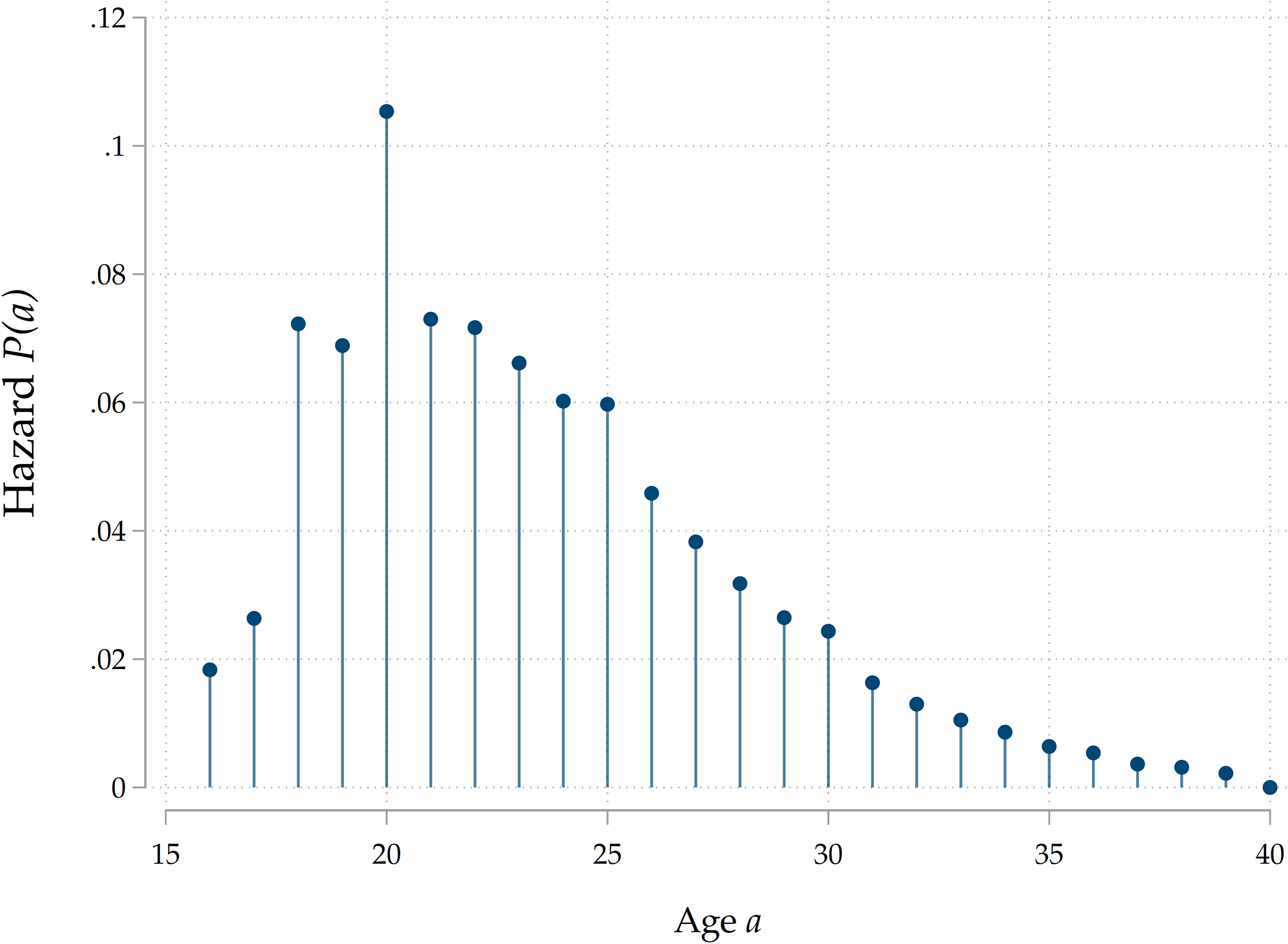
Figure B.2. Home-leaving hazard in the analytical sample.

Figure B.3. Home-leaving survival in the analytical sample.
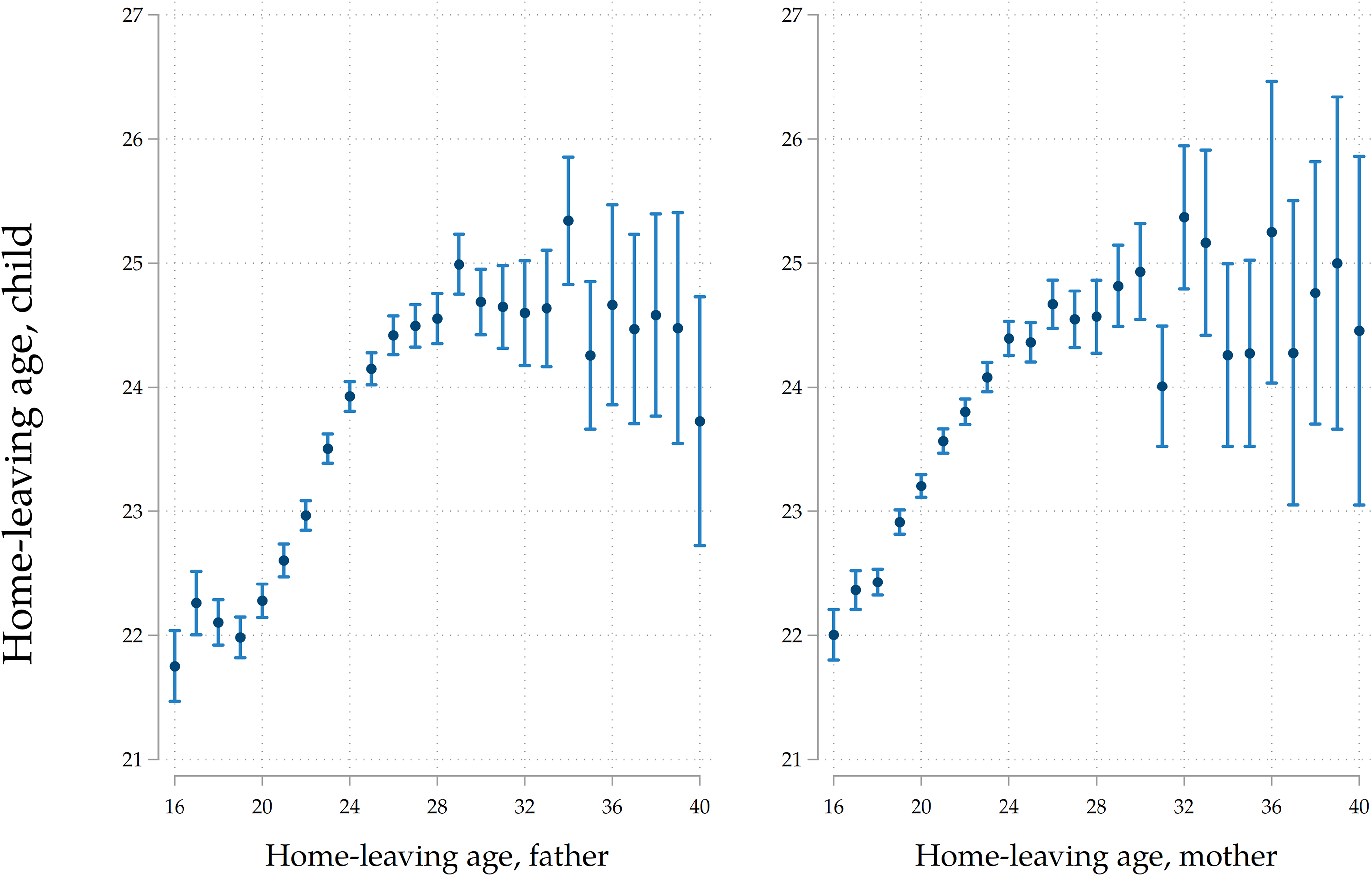
Figure B.4. Average home-leaving age of parents and their children.
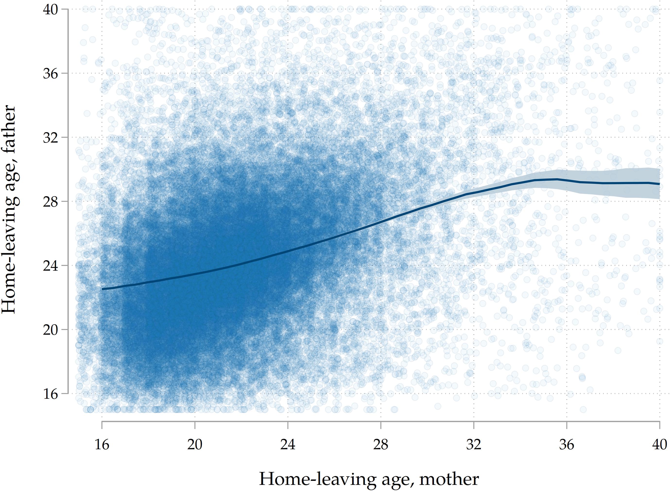
Figure B.5. Association between paternal and maternal home-leaving ages.
Note: Each dot represents the home-leaving ages of a father-mother couple from G1. The overlaid blue line displays fitted values from a kernel-weighted local polynomial regression with 99% confidence intervals. Since information on home-leaving ages is discrete with yearly increments, we add spherical random noise to each datapoint to aid visualization.

Figure B.6. Intergenerational transmission of socio-economic background.

Figure B.7. Intergenerational transmission of education.

Figure B.8. Parental education and occupation.
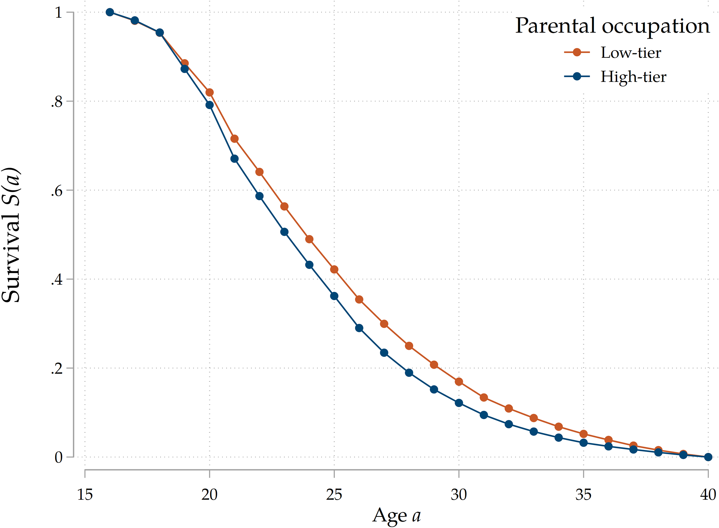
Figure B.9. Parental occupation and children home-leaving ages.
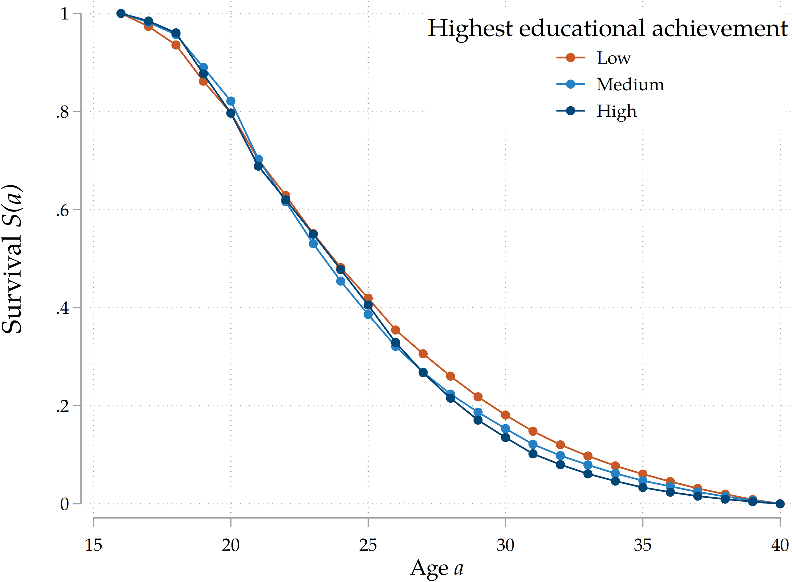
Figure B.10. Education and children home-leaving ages.
C. Results from logit models
Table 2. Estimation results from logit models

Note: Estimated coefficients from various logit models (2) estimated on the entire sample with at least on responding parent.
 $Female$
is a dummy that denotes the sex of the adult child; similarly,
$Female$
is a dummy that denotes the sex of the adult child; similarly,
 $Mother$
denotes the gender of the responding parent. For brevity, we omit the coefficients on the triple interaction between country groups,
$Mother$
denotes the gender of the responding parent. For brevity, we omit the coefficients on the triple interaction between country groups,
 ${T}_{Par}$
and
${T}_{Par}$
and
 $Mother$
.
$Mother$
.
 $LeftOthe{r}_{Par}$
is a dummy equal to one if the home-leaving decision of the parent was not related to family formation. Asterisks next to coefficients denote statistical significance at the 10% ( * ), 5% ( ** ), and 1% ( *** ) levels.
$LeftOthe{r}_{Par}$
is a dummy equal to one if the home-leaving decision of the parent was not related to family formation. Asterisks next to coefficients denote statistical significance at the 10% ( * ), 5% ( ** ), and 1% ( *** ) levels.
D. Additional figures: results

Figure D.11. Results by sex of adult child, all specifications.
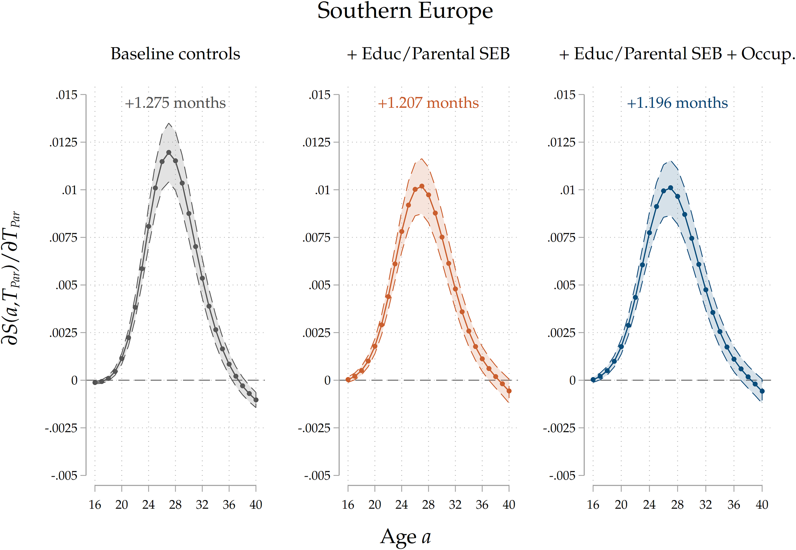
Figure D.12. Results for Southern European countries, all specifications.

Figure D.13. Results for Western European countries, all specifications.

Figure D.14. Results for Northern European countries, all specifications.
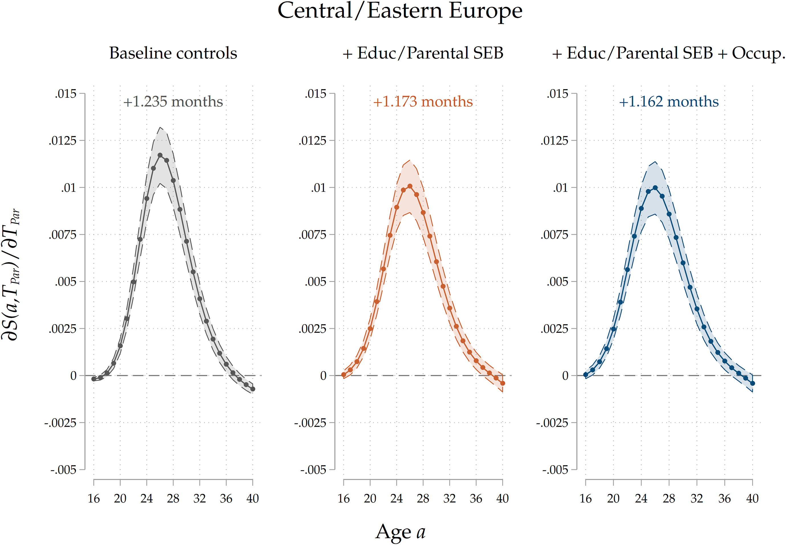
Figure D.15. Results for Central/Eastern European countries, all specifications.
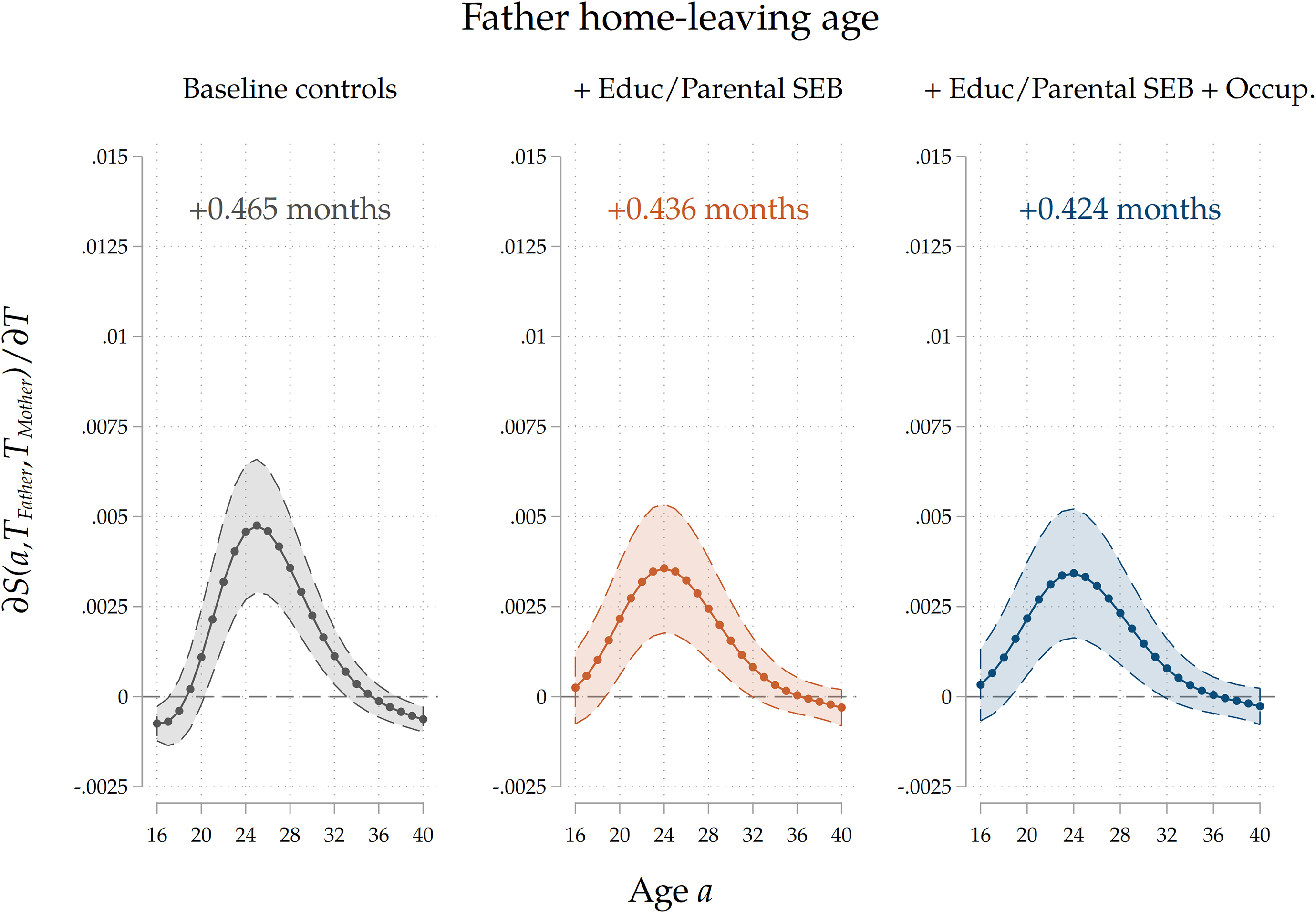
Figure D.16. Results for father home-leaving age, all specifications.

Figure D.17. Results for mother home-leaving age, all specifications.
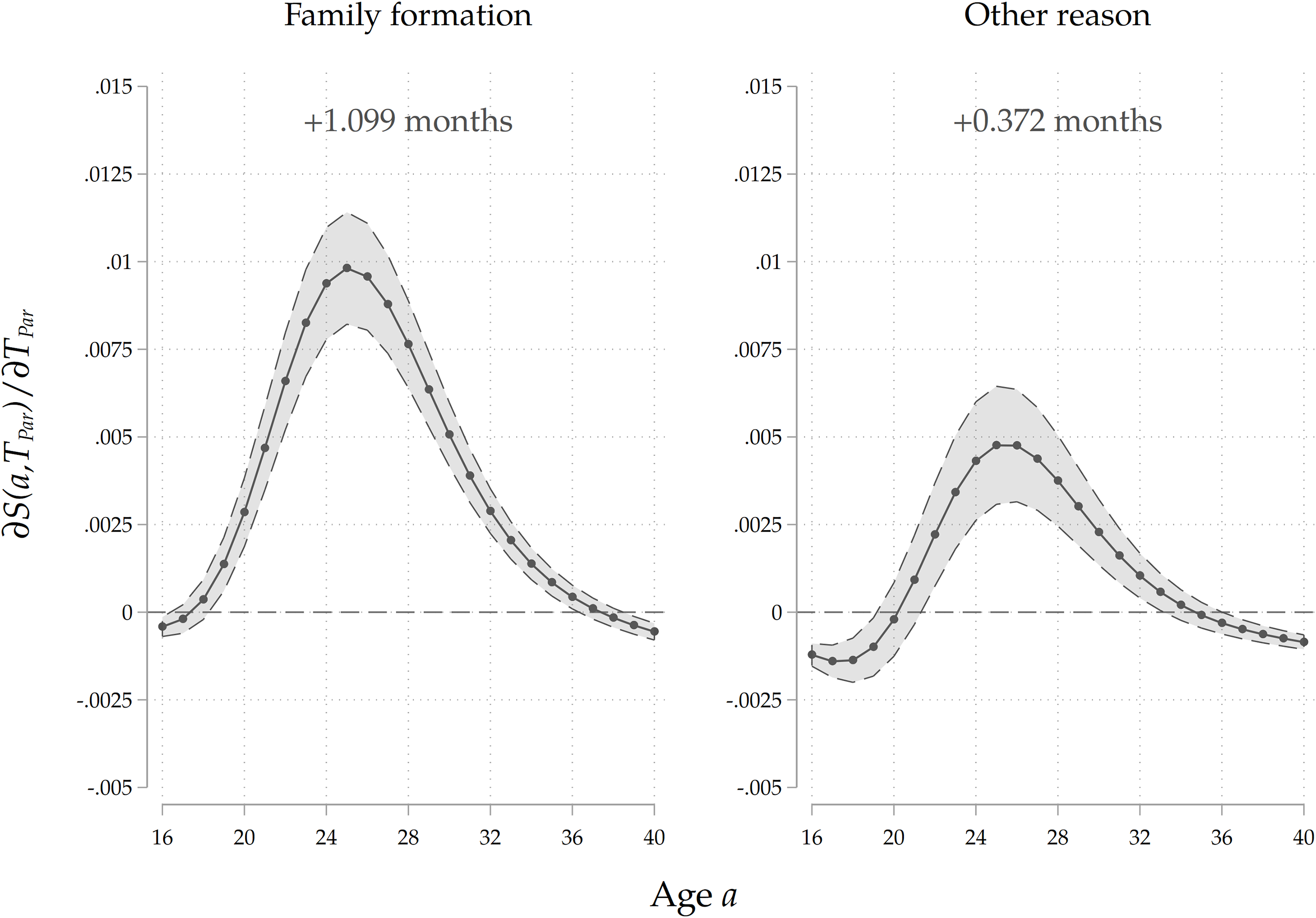
Figure D.18. Results by parental reason for leaving home, first specification.

Figure D.19. Results by parental reason for leaving home, second specification.
E. Additional figures: robustness

Figure E.20. Results from the cubic polynomial specification, entire sample.

Figure E.21. Results for the subsample with information on both parents’ home-leaving ages.

Figure E.22. Results from the hazard model, entire sample.
Note: The Figure displays average marginal effects of an 1-year increase in
 ${T}_{Par}$
on
${T}_{Par}$
on
 $\mathbb{E}\left({H}_{it}\right)=\rm{P}\rm{r}({H}_{it}=1)$
, i.e., it plots
$\mathbb{E}\left({H}_{it}\right)=\rm{P}\rm{r}({H}_{it}=1)$
, i.e., it plots
 $\widehat{\partial H\left(a\right)/\partial {T}_{Par}}$
(as well as its 95% confidence intervals for each marginal effect) for each value of age
$\widehat{\partial H\left(a\right)/\partial {T}_{Par}}$
(as well as its 95% confidence intervals for each marginal effect) for each value of age
 $a\in \{\rm{16,17}, \ldots, 40\}$
. Standard errors are clustered at the family level.
$a\in \{\rm{16,17}, \ldots, 40\}$
. Standard errors are clustered at the family level.
F. Information on occupations
Information on occupational status is collected in SHARE in different ways across different waves. In wave 1, if they are not retired, people are asked about their job title for both their main (ep016_1) and secondary job (ep016_2), if they have one. If they are retired, they are asked about the job title for their last job before retirement (ep052). Information obtained in wave 1 has been recoded according to the ISCO-88 classification of occupations at a 4-digit detail level, and it is contained in the variables isco_1job, isco_2job and isco_ljob contained in the gv-isced module. Moreover, in wave 1 people also report the last job their mothers and fathers had (dn029-1 and dn029-2): also these are recoded according to a 4-digit ISCO-88 scale and are part of the gv-isced module under the names isco_fa (for fathers) and isco_mo (for fathers). We completely disregard the information on secondary jobs, assuming that the best measure of occupational attainment is the job title on the main job. In waves 2, 4 and 5 this information is collected again (for the main or last job) but it is recoded according to the ISCO-08 classification of occupations at a 1-digit detail level. We keep the information from the most recent wave in which each respondent reports about the main/last job, to keep into account potential job switches in later stages of the working life Table 3 contains the distribution of occupations among members of G1, the generation of parents.
Table 3. Distribution of occupations among responding parents (G1)
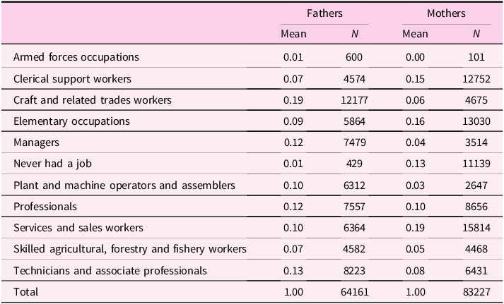
Note: occupations are defined according to the ISCO 1-digit aggregation level. We add a residual category for those who report having never worked.
G. Estimand and empirical models
Our estimate of interest is
 $\partial T/\partial {T}_{Par}$
. In this Section, we show that under some assumptions of the period of exposure to the risk of home-leaving, it is possible to map the estimates from a discrete-time model of the survival function into marginal effects on average survival. It is well known (and we show it again in Appendix G.3 that this cannot be done in models that use the hazard
$\partial T/\partial {T}_{Par}$
. In this Section, we show that under some assumptions of the period of exposure to the risk of home-leaving, it is possible to map the estimates from a discrete-time model of the survival function into marginal effects on average survival. It is well known (and we show it again in Appendix G.3 that this cannot be done in models that use the hazard
 ${H}_{it}$
a dependent variable. This motivates our choice of the survival-based model to obtain the main results, which are more easily interpretable in terms of home-leaving ages.
${H}_{it}$
a dependent variable. This motivates our choice of the survival-based model to obtain the main results, which are more easily interpretable in terms of home-leaving ages.
G.1. Effect on average age at home-leaving
Assume that there exist
 $\underline{a},\overline{a}\in \mathbb{N}$
such that
$\underline{a},\overline{a}\in \mathbb{N}$
such that
 $S\left(\underline{a}\right)=1$
and
$S\left(\underline{a}\right)=1$
and
 $S\left(\overline{a}\right)=0$
, and we denote
$S\left(\overline{a}\right)=0$
, and we denote
 ${\mathcal{A}}= \{{\it \underline{a}},{\it \underline{a}}+ 1, \ldots, {\it \overline{a}}-1,{\it \overline{a}\overline{}}\}$
. Let
${\mathcal{A}}= \{{\it \underline{a}},{\it \underline{a}}+ 1, \ldots, {\it \overline{a}}-1,{\it \overline{a}\overline{}}\}$
. Let
 $T$
denote the average home-leaving age, given by
$T$
denote the average home-leaving age, given by
 $$T=\sum _{\underline{a}\le a \lt \overline{a}}\,P\left(a\right)\cdot a,$$
where
 $P\left(a\right)=\rm{P}\rm{r}(T={\it a})$
. Given that
$P\left(a\right)=\rm{P}\rm{r}(T={\it a})$
. Given that
 $$P\left(a\right)=S\left(a\right)-S(a+1),$$
where
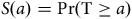 $S\left(a\right)=\rm{P}\rm{r}(T\ge {\it a})$
, it is possible to write
$S\left(a\right)=\rm{P}\rm{r}(T\ge {\it a})$
, it is possible to write
which simplifies to
 $$T=\underline{a}+\sum _{\underline{a} \lt a \lt \overline{a}}\,S\left(a\right),$$
and therefore that
 $${{\partial T} \over {\partial {T_{Par}}}} = \mathop \sum \limits_{\underline a \lt a \lt \overline{a}} {{\partial S\left( {a,{T_{Par}}} \right)} \over {\partial {T_{Par}}}}$$
Therefore, once we have estimated the marginal effect of
 ${T}_{Par}$
on
${T}_{Par}$
on
 $S$
for all
$S$
for all
 $a$
, it is possible to back up the marginal effect of
$a$
, it is possible to back up the marginal effect of
 ${T}_{Par}$
on
${T}_{Par}$
on
 $T$
.
$T$
.
G.2. Estimation details
In our setting, we have that
 $\underline{a}=16$
and
$\underline{a}=16$
and
 $\overline{a}=40$
. We estimate the following empirical specification:
$\overline{a}=40$
. We estimate the following empirical specification:
 $$\mathbb{E}\left( {{S_{it}}} \right) = {{{\rm{exp}}\left( {\mathop \sum \nolimits_{j = 0}^k {\alpha _j}Age_{i,t}^j + \mathop \sum \nolimits_{j = 0}^k \,{\beta _j}\left( {{T_{Par,i}} \times Age_{i,t}^j} \right) + \gamma {\rm{'}}{{\bf{X}}_{it}} + {\eta _t}} \right)} \over {1 + {\rm{exp}}\left( {\mathop \sum \nolimits_{j = 0}^k {\alpha _j}Age_{i,t}^j + \mathop \sum \nolimits_{j = 0}^k \,{\beta _j}\left( {{T_{Par,i}} \times Age_{i,t}^j} \right) + \gamma {\rm{'}}{{\bf{X}}_{it}} + {\eta _t}} \right)}}.$$
After estimation, we obtain the average marginal effects
 ${{\partial S\left( {a|{T_{Par}}} \right)} \over {\partial {T_{Par}}}}$
for
${{\partial S\left( {a|{T_{Par}}} \right)} \over {\partial {T_{Par}}}}$
for
 $a\in \{\rm{16,17}, \ldots, 40\}$
. Notice, that by construction since
$a\in \{\rm{16,17}, \ldots, 40\}$
. Notice, that by construction since
 $S\left(16\right)=1$
and
$S\left(16\right)=1$
and
 $S\left(40\right)=0$
are constant, we should have
$S\left(40\right)=0$
are constant, we should have
 $${{\partial S\left( {16|{T_{Par}}} \right)} \over {\partial {T_{Par}}}} = {{\partial S\left( {40|{T_{Par}}} \right)} \over {\partial {T_{Par}}}} = 0.$$
In practice, if use a polynomial approximation of the survival function it might be that our estimated baseline survival
 $\widehat{S}\left(a\right)$
is such that
$\widehat{S}\left(a\right)$
is such that
 $\widehat{S}\left(16\right)\ne 1$
and
$\widehat{S}\left(16\right)\ne 1$
and
 $\widehat{S}\left(40\right)\ne 0$
. For the same reason, it might be that
$\widehat{S}\left(40\right)\ne 0$
. For the same reason, it might be that
 ${{\partial \hat S\left( {16|{T_{Par}}} \right)} \over {\partial {T_{Par}}}} \ne 0$
or
${{\partial \hat S\left( {16|{T_{Par}}} \right)} \over {\partial {T_{Par}}}} \ne 0$
or
 ${{\partial \hat S\left( {40|{T_{Par}}} \right)} \over {\partial {T_{Par}}}} \ne 0$
, or both. As this is clearly due to the parametric restrictions we imposed, when computing the expected home-leaving age using (4) we assume that
${{\partial \hat S\left( {40|{T_{Par}}} \right)} \over {\partial {T_{Par}}}} \ne 0$
, or both. As this is clearly due to the parametric restrictions we imposed, when computing the expected home-leaving age using (4) we assume that
 ${{\partial \hat S\left( {16|{T_{Par}}} \right)} \over {\partial {T_{Par}}}} = {{\partial \hat S\left( {40|{T_{Par}}} \right)} \over {\partial {T_{Par}}}} = 0$
. Indeed, when estimating a model with age dummies that allows for a flexible specification of the baseline survival
${{\partial \hat S\left( {16|{T_{Par}}} \right)} \over {\partial {T_{Par}}}} = {{\partial \hat S\left( {40|{T_{Par}}} \right)} \over {\partial {T_{Par}}}} = 0$
. Indeed, when estimating a model with age dummies that allows for a flexible specification of the baseline survival
 $S\left(a\right)$
, we find that the derivative of the survival function at
$S\left(a\right)$
, we find that the derivative of the survival function at
 $a\in \left\{\rm{16,40}\right\}$
is not estimable, as we only have individuals who are still at home (for
$a\in \left\{\rm{16,40}\right\}$
is not estimable, as we only have individuals who are still at home (for
 $a=16$
) or that already left (for
$a=16$
) or that already left (for
 $a=40$
). Therefore, we have to rely on a polynomial approximation of degree
$a=40$
). Therefore, we have to rely on a polynomial approximation of degree
 $k$
. As our numerical results on
$k$
. As our numerical results on
 $\widehat {{{\partial T} \over {\partial {T_{Par}}}}}$
are sensitive to the choice of
$\widehat {{{\partial T} \over {\partial {T_{Par}}}}}$
are sensitive to the choice of
 $k$
, we pick
$k$
, we pick
 $k=2$
but perform a robustness test in which we estimate the baseline model for
$k=2$
but perform a robustness test in which we estimate the baseline model for
 $k=3$
.
$k=3$
.
G.3 Derivative of hazard and average home-leaving ages
In this Subsection, I show that by modeling the hazard rate instead of the survival function, it is impossible to pin down
 ${{\partial T} \over {\partial {T_{Par}}}}$
. Start by noticing that
${{\partial T} \over {\partial {T_{Par}}}}$
. Start by noticing that
 $$\rm{P}\rm{r}\left(T={\it a}|{T}_{\it Par}\right)={\it S}\left({\it a}\right|{\it T}_{\it Par}\left){\it H}\right({\it a}\left|{\it T}_{\it Par}\right).$$
Therefore, since
 $$S\left(a\right|{T}_{Par})=1-\sum _{t \lt a}\,\rm{P}\rm{r}({\it T}={\it t}\left|{\it T}_{\it Par}\right),$$
we can write
 $$\rm{P}\rm{r}\left({\it T}={\it a}|{\it T}_{\it Par}\right)=\left(1-\sum _{\it t \lt a}\,\rm{P}\rm{r}({\it T=t}|{\it T}_{\it Par})\right){\it H}\left(\it a\right|{\it T}_{\it Par}).$$
Hence, we have that
 $${{\partial {\rm{Pr}}\left( {\it T = a|{T_{Par}}} \right)} \over {\partial {\it T_{Par}}}} = \left( {1 - \sum\limits_{\it t \lt a} {\mkern 1mu} {{\partial {\rm{Pr}}({\it T = t}|{\it T_{Par}})} \over {\partial {\it T_{Par}}}}} \right){\it H}({\it a}|{\it T_{Par}}) + \left( {1 - \sum\limits_{{\it t} \lt {\it a}} {\mkern 1mu} {\rm{Pr}}({\it T = t}|{\it T_{Par}})} \right){{\partial {\it H(a|{T_{Par}})}} \over {\partial {\it T_{Par}}}}.$$
We can therefore obtain
 $\partial T/\partial {T}_{Par}$
through an iterative procedure. First, notice that
$\partial T/\partial {T}_{Par}$
through an iterative procedure. First, notice that
 $$\rm{P}\rm{r}\left({\it T=\underline{a}|{T}_{Par}}\right)={\it S}\left({\it \underline{a}|{T}_{Par}}\right){\it H}\left({\it \underline{a}}\right|{\it T}_{\it Par}\left)\stackrel{\it S\left(\it \underline{a}\right)=1}{=}{\it H}\right({\it \underline{a}}\left|{\it T}_{\it Par}\right).$$
We therefore have that
 $${{\partial {\rm{Pr}}\left( {T = \underline a |{T_{Par}}} \right)} \over {\partial {T_{Par}}}} = {{\partial (\underline a |{T_{Par}})} \over {\partial {T_{Par}}}}.$$
For
 $a=\underline{a}+1$
, we have
$a=\underline{a}+1$
, we have

This shows that it is not possible to obtain the effects on the mean survival time after estimating the derivative of the hazard function with respect to
 ${T}_{Par}$
, as we also need the baseline probabilities which are not estimated.
${T}_{Par}$
, as we also need the baseline probabilities which are not estimated.


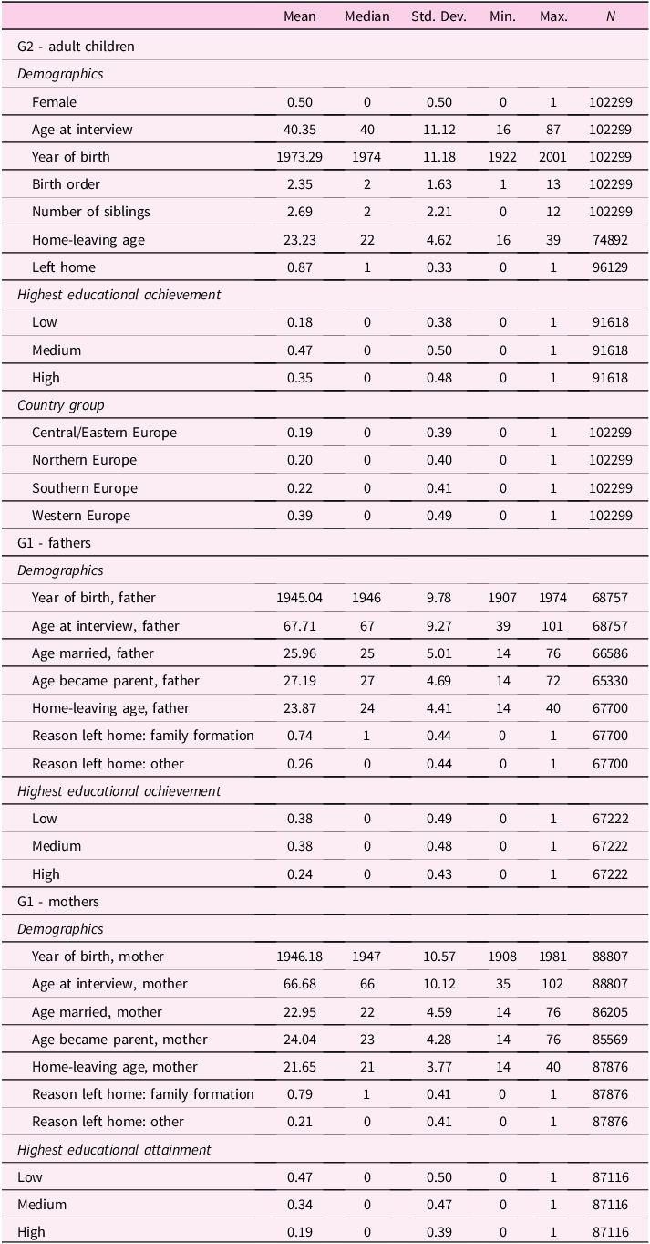

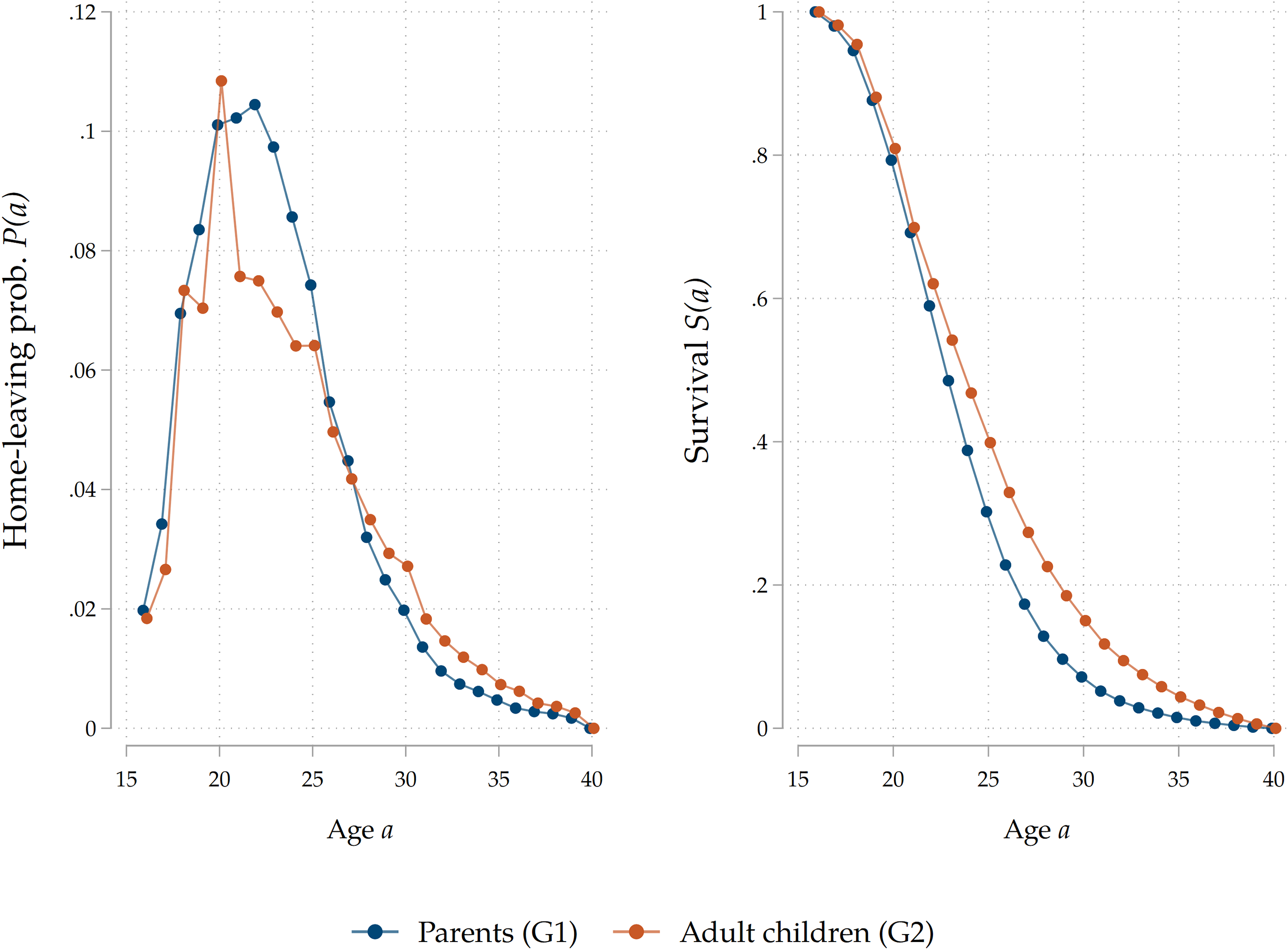

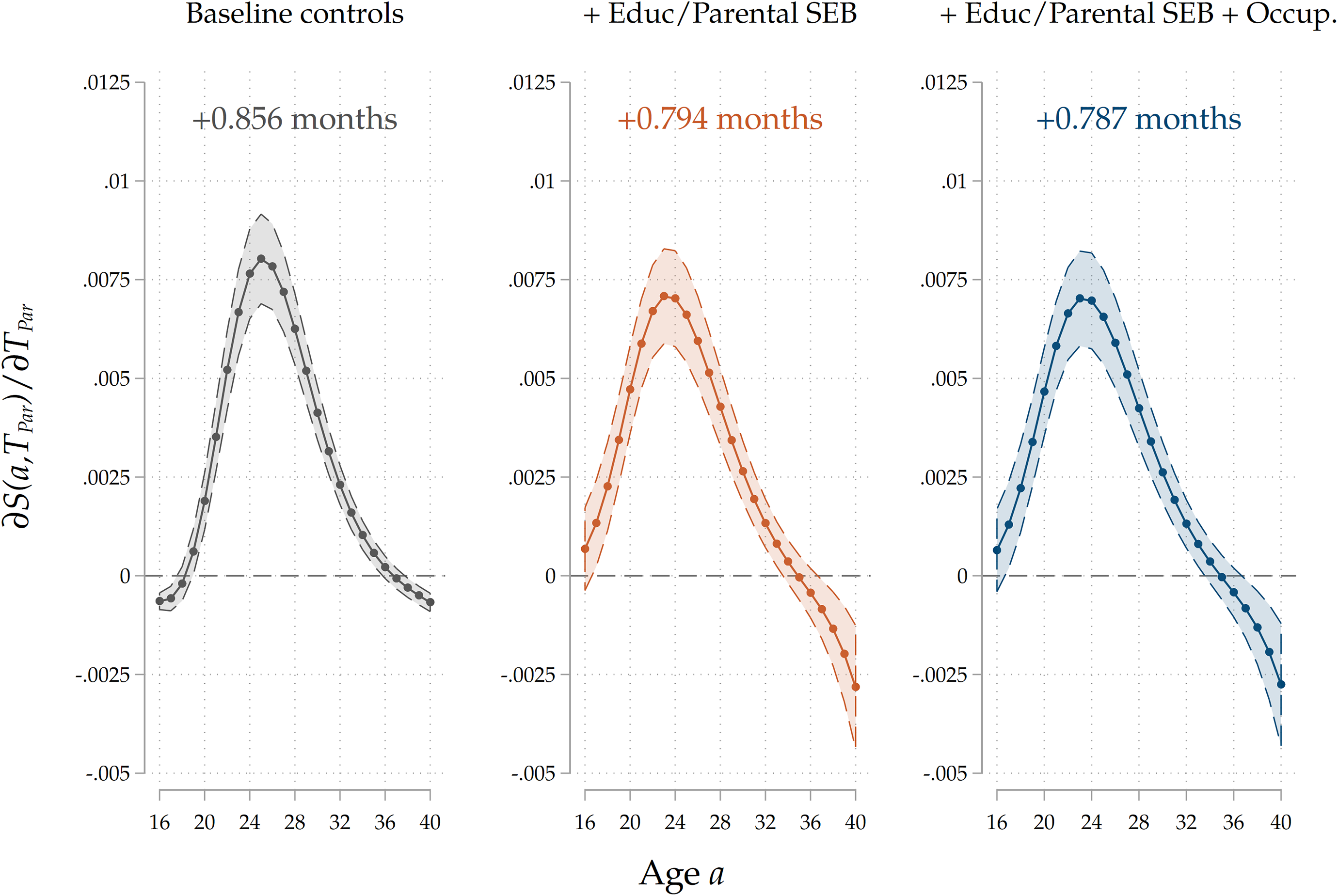


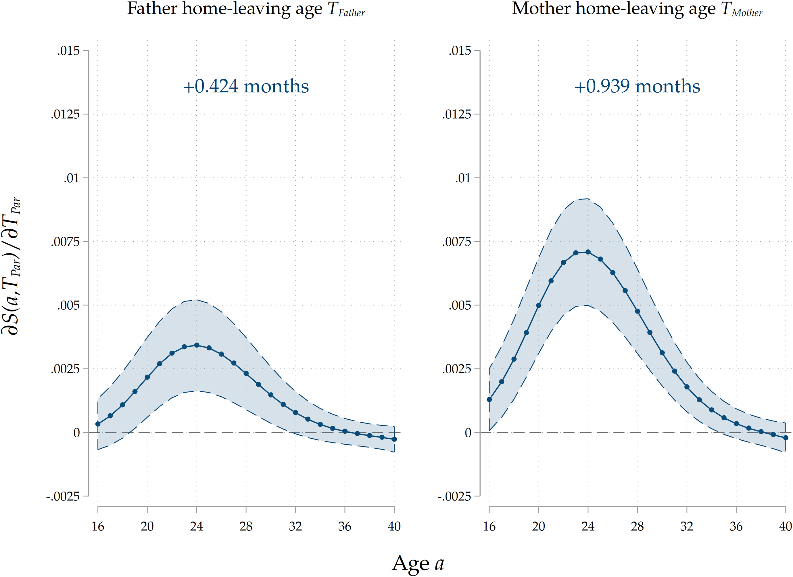


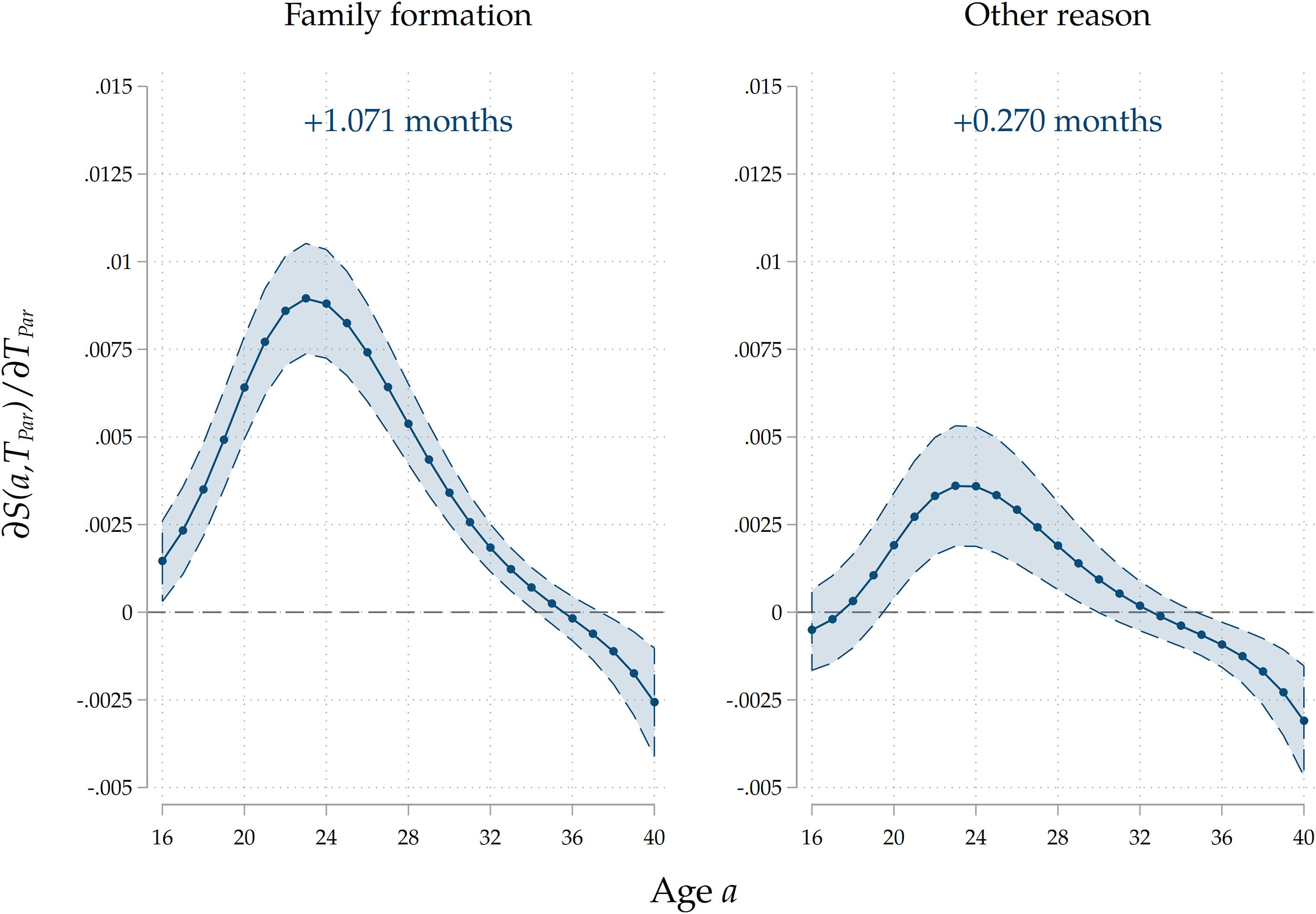


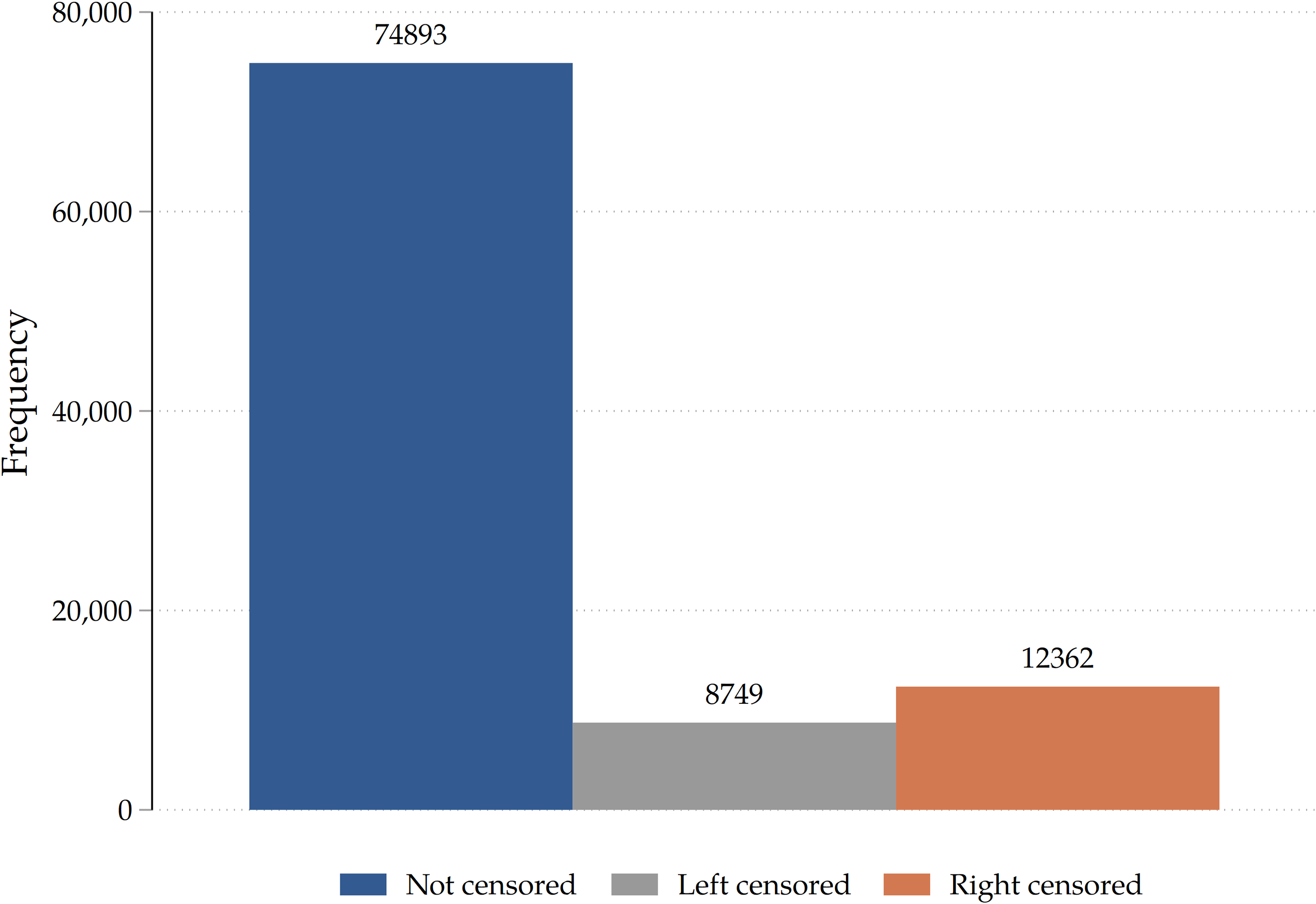

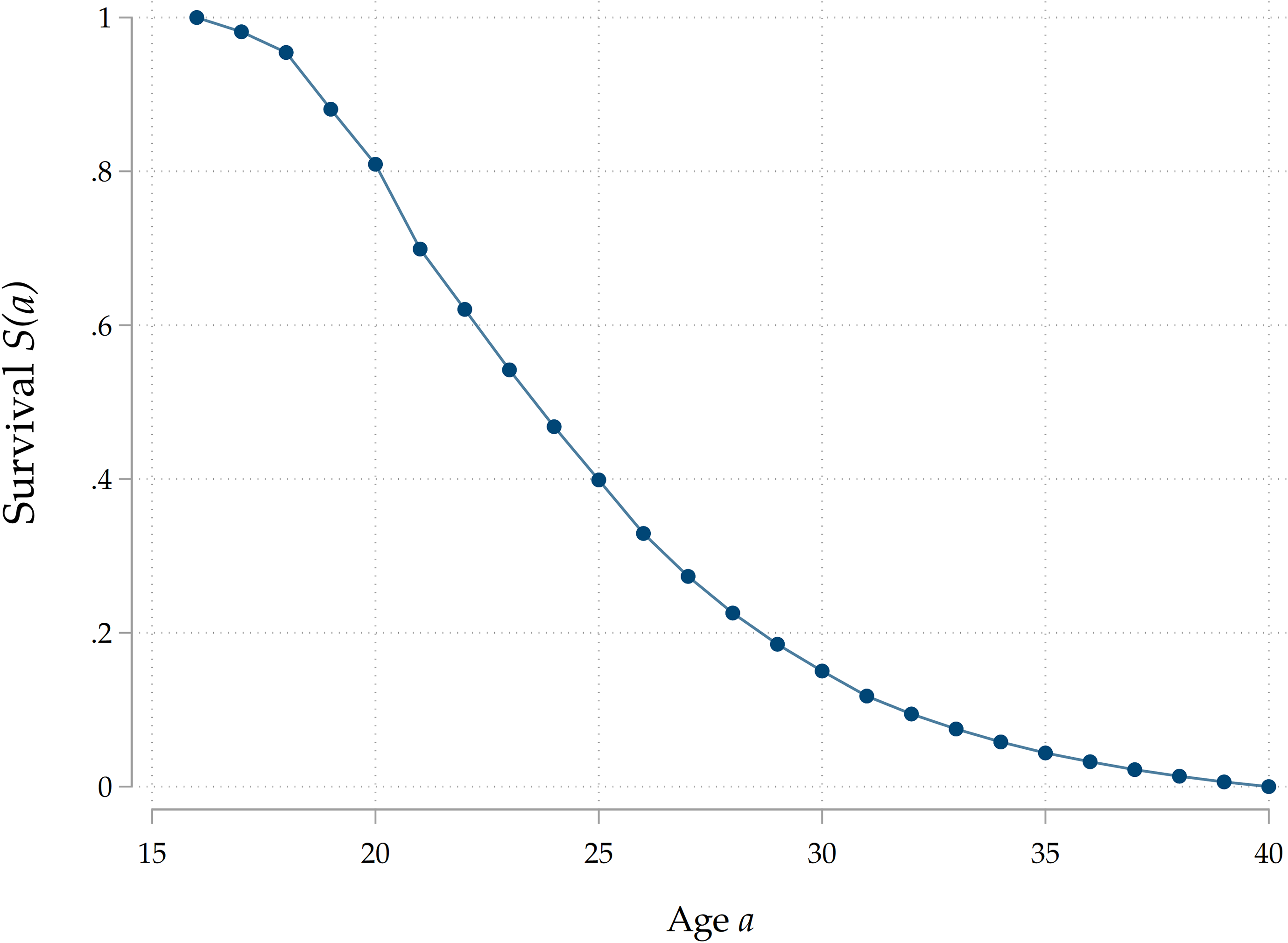


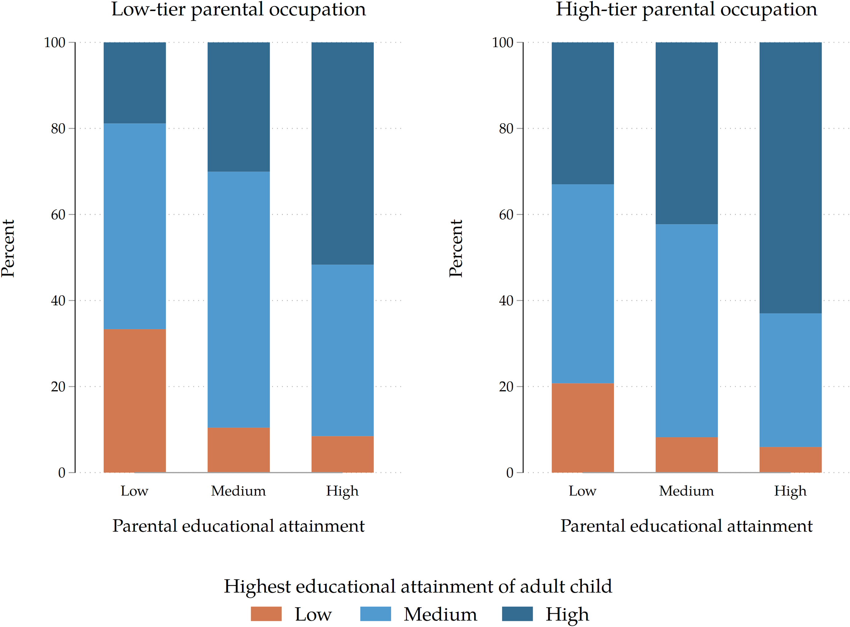
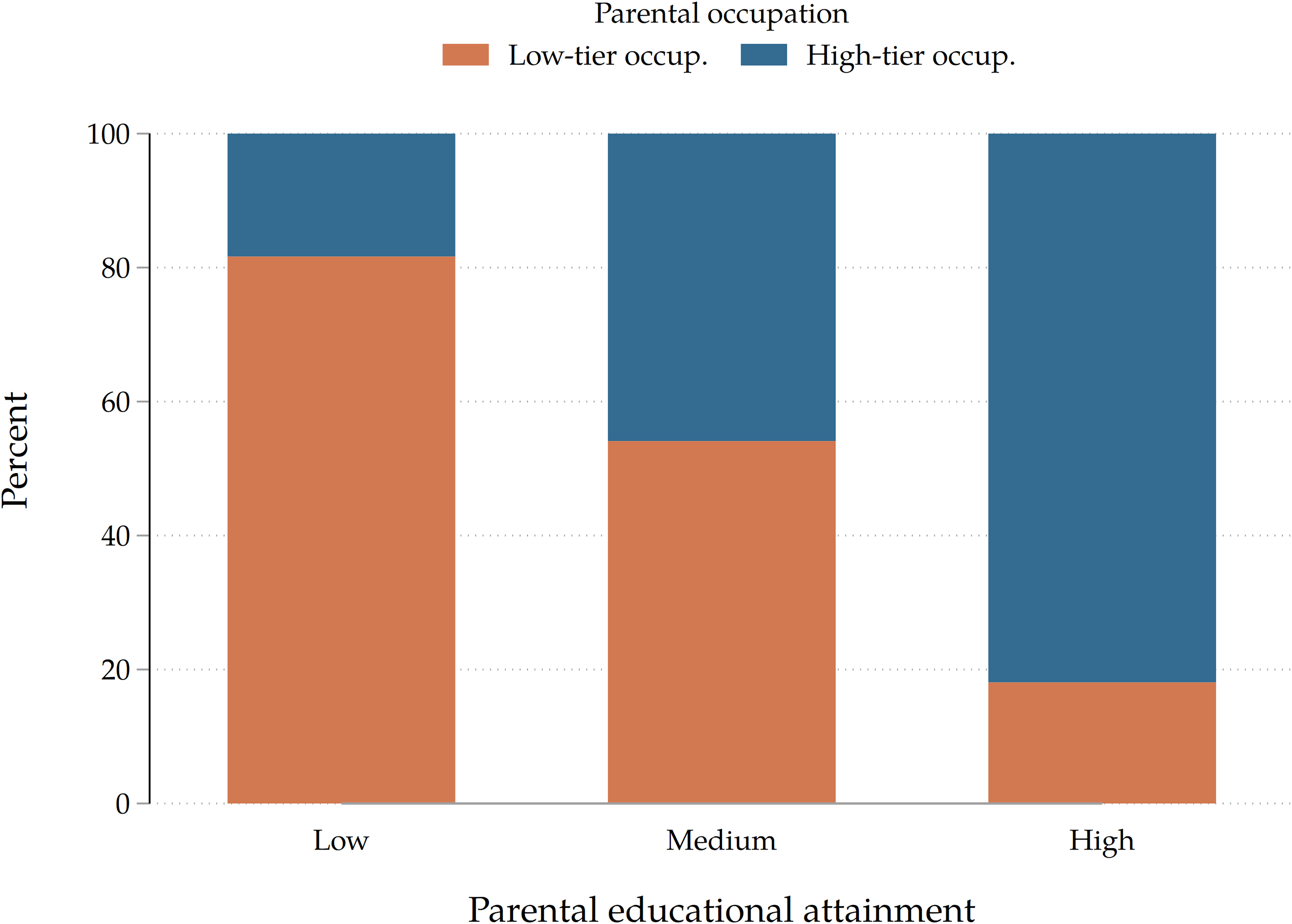


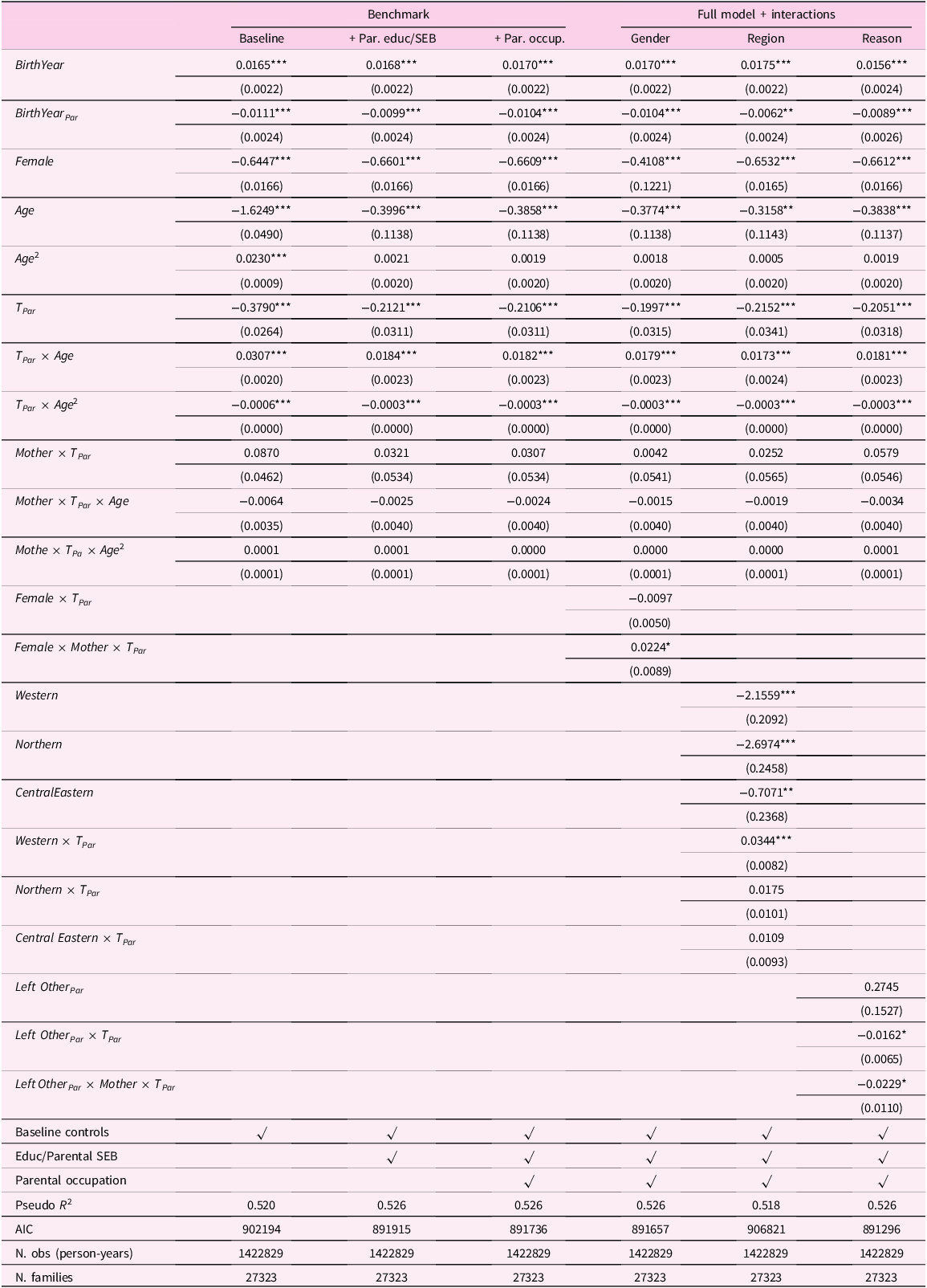
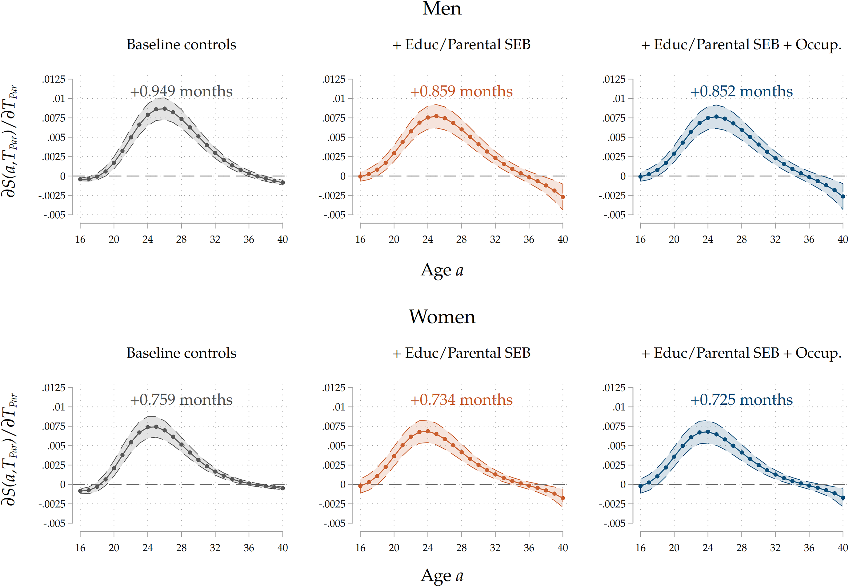

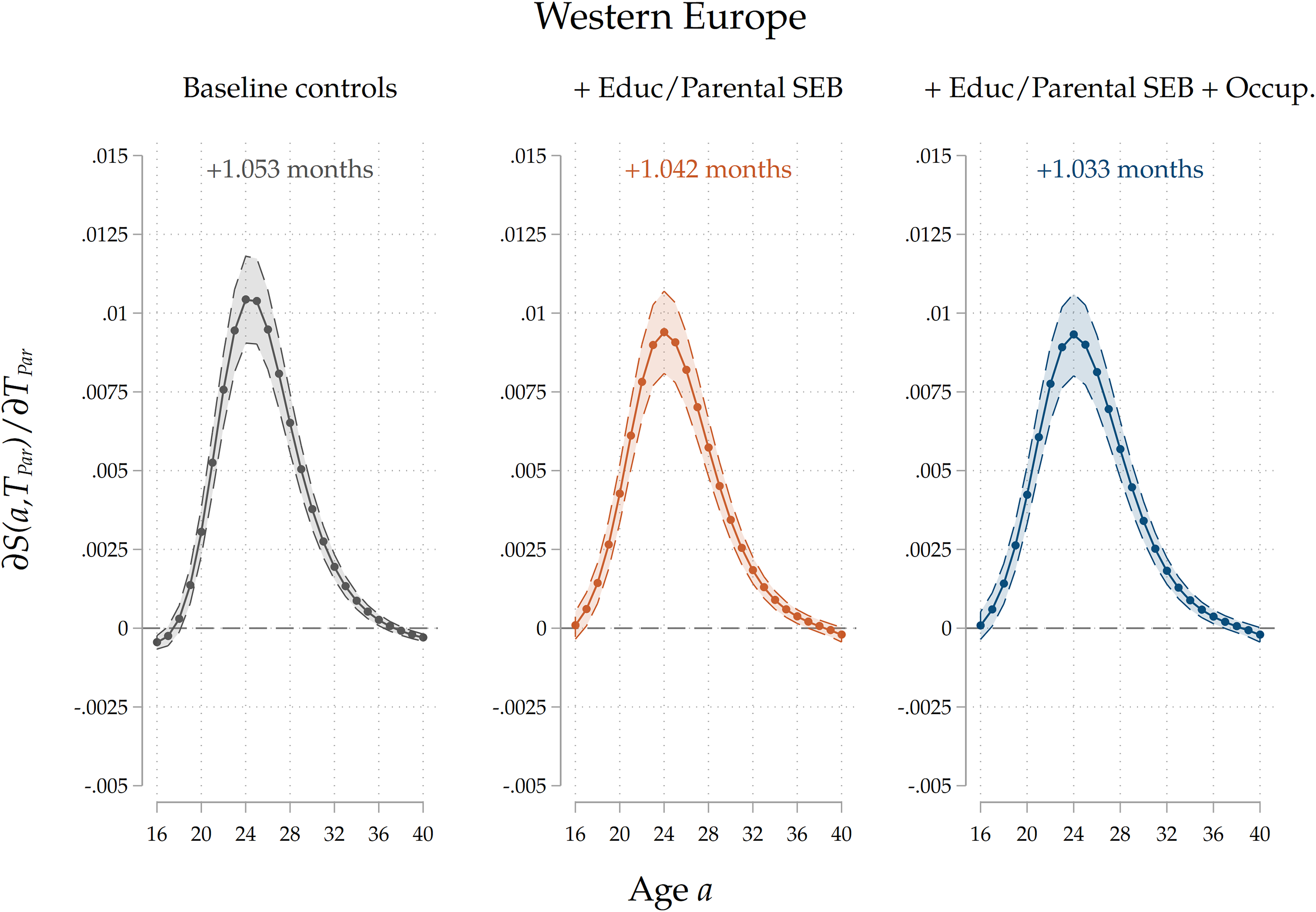
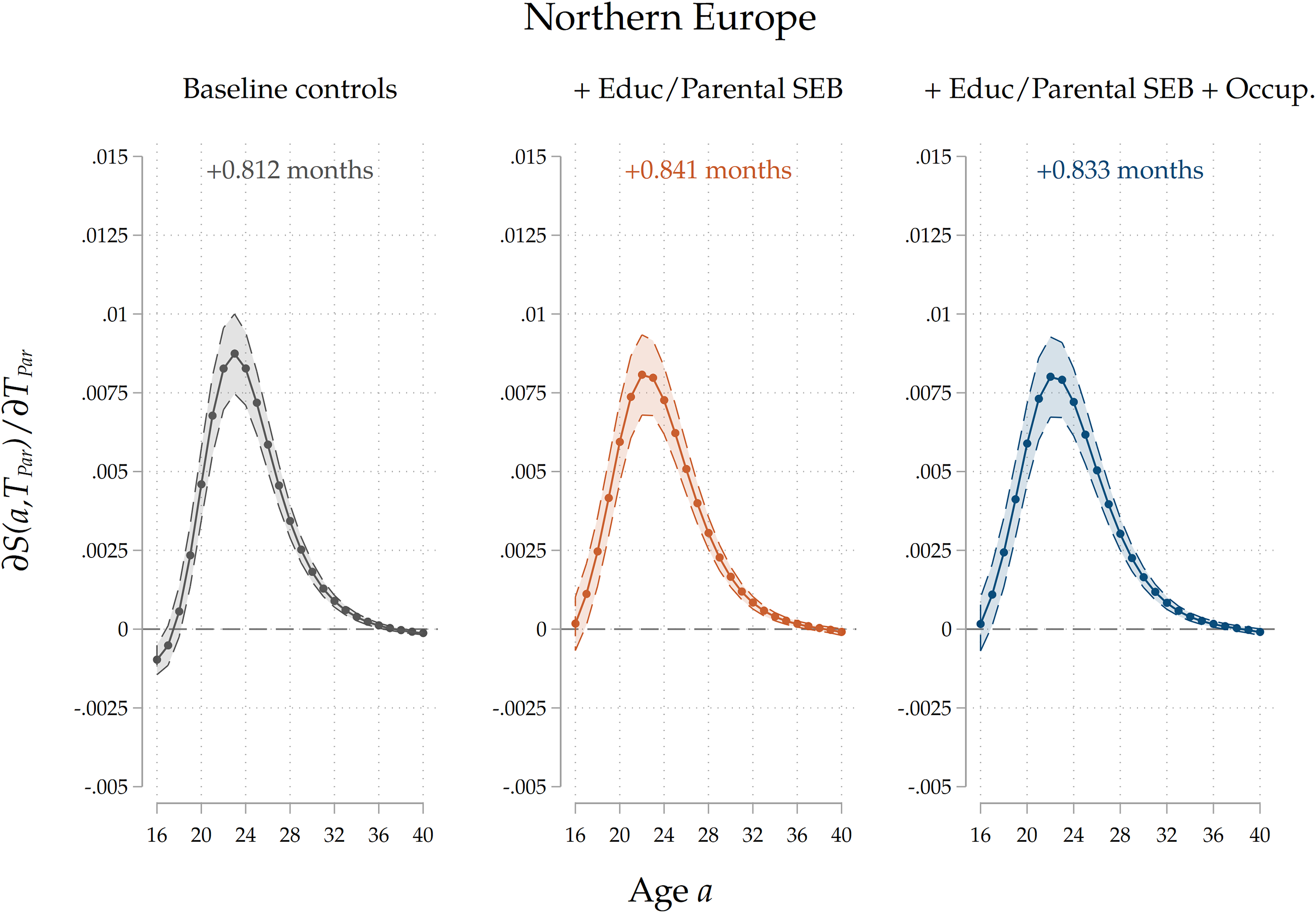


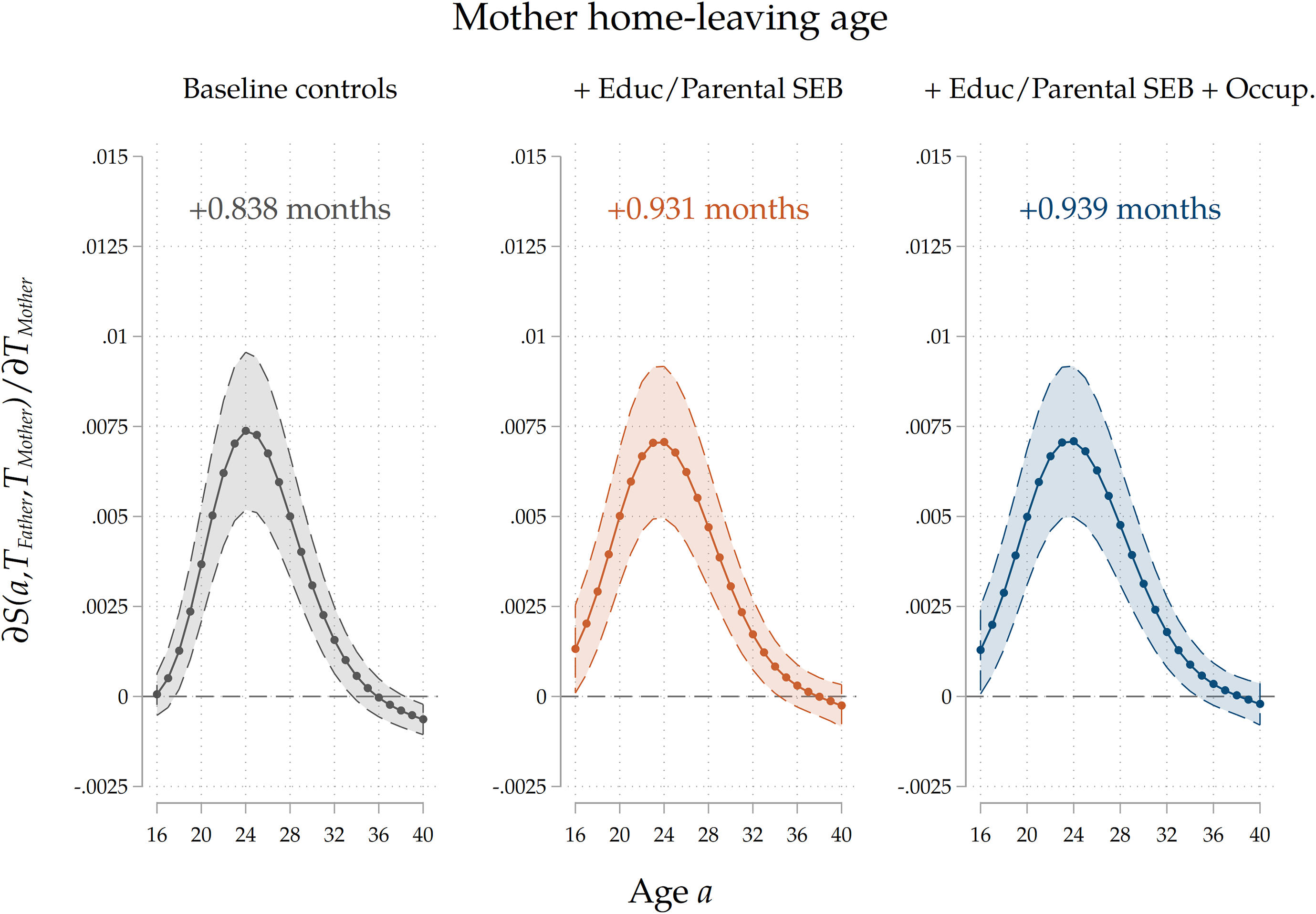

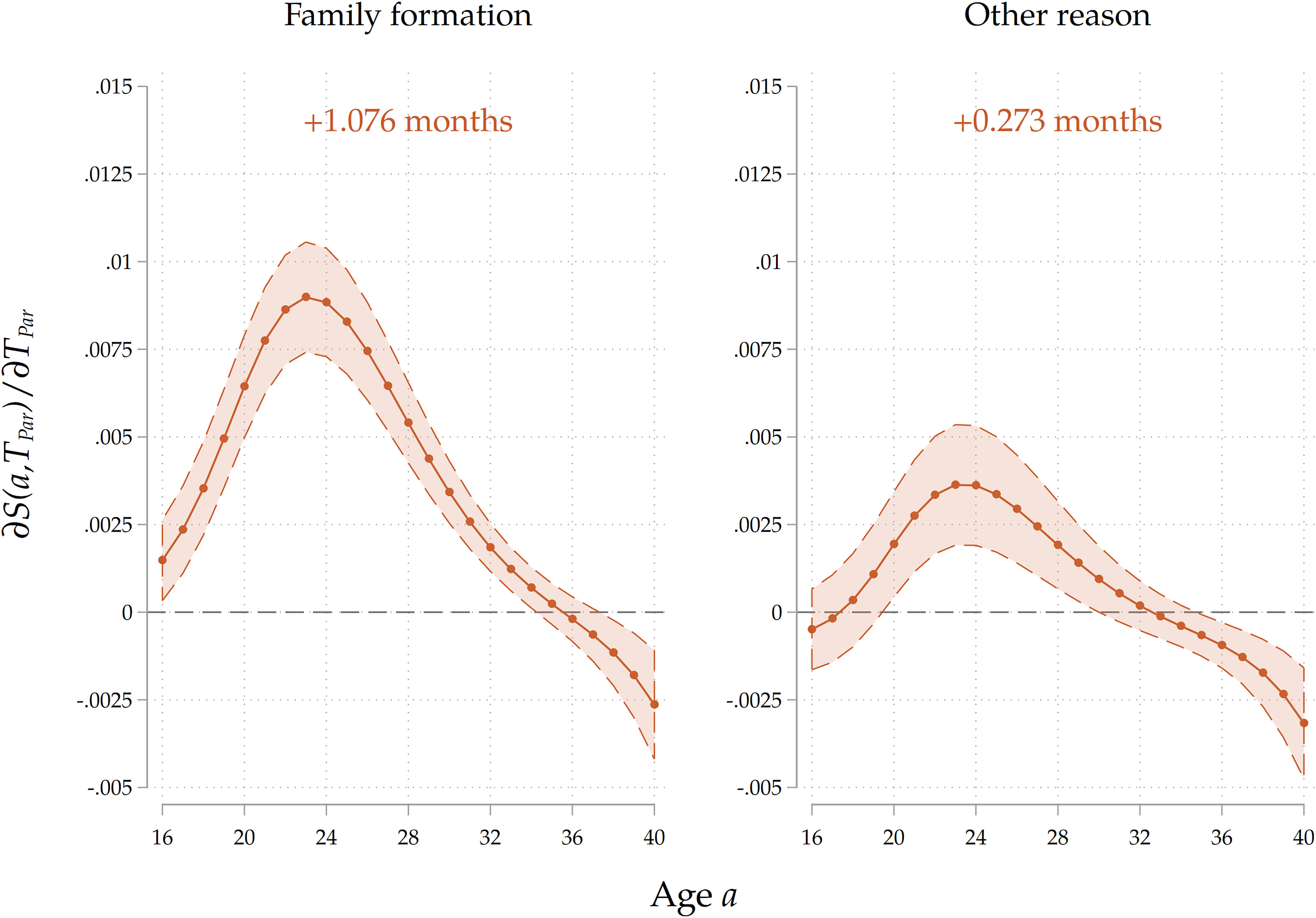
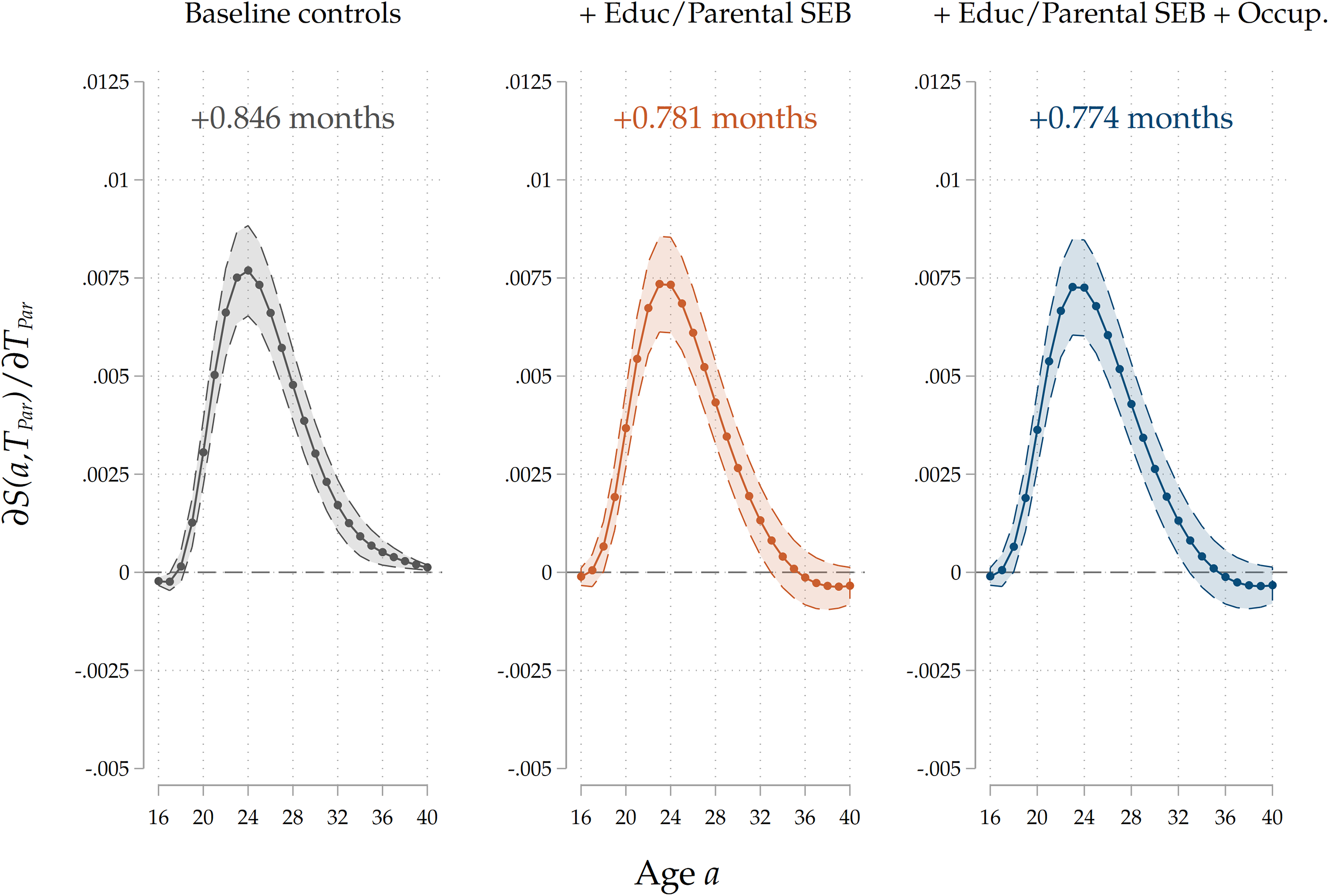
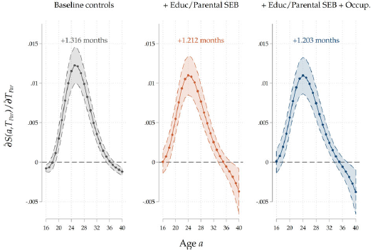
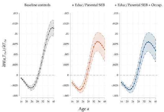


 Open access