


Impact Statement
In line with sustainable aviation goals, prolific research is being conducted into propeller-driven aircraft. Designs featuring a conventional tractor–propeller configuration typically have 40 % of their lifting surface area immersed in the propeller slipstream. This fraction of area is expected to increase with the development of distributed propulsion systems, which feature multiple propulsors mounted along the span of a lifting surface. The propeller slipstream encountered by the lifting surface is highly unsteady, encompassing a helical system of blade tip and wake vorticity. This vortical system convects over the downstream lifting surface, where it undergoes a cyclic interaction with the developing boundary layer. The unsteady interaction can affect lifting surface performance through local vortex-induced separation of the boundary-layer flow, although this has received limited attention in the literature. Hence, the objective of our work is a quantification of the flow topology associated with the vorticity–boundary-layer interaction and the underlying mechanisms driving incipient, local separation of the boundary layer. Particularly, we resolve all three velocity components in a three-dimensional (3-D) volume encompassing the near-wall advection of the propeller tip vortices, where the concentration of the helical vorticity is expected to cause the strongest adverse interaction with the turbulent boundary layer.
1. Introduction
The growing volume and footprint of air traffic has been motivating the development of more sustainable aircraft (Bonet et al. Reference Bonet, Schellenger, Rawdon, Elmer, Wakayama, Brown and Guo2011). Within these development efforts there has been revived interest in propeller-driven aviation, with modern advancements in propeller-blade design and integration proposing up to 10 %–30 % in fuel savings as compared with the best engines in service (Atanasov et al. Reference Atanasov, Wehrspohn, Kühlen, Cabac, Silberhorn, Kotzem, Dahlmann and Linke2023; Guynn et al. Reference Guynn, Berton, Haller, Hendricks and Tong2012). Their scalability also allows for a multitude of smaller propellers to be combined with emerging hybrid-electric propulsion technology, featured in numerous development programs for next-generation aircraft (De Vries et al. Reference De Vries, Brown and Vos2019; Deere et al. Reference Deere, Viken, Carter, Viken, Wiese and Farr2017). However, the challenge with these configurations still lies in the optimal integration of the propeller onto the airframe, as well as reducing the relatively higher noise levels. Historically, and in modern aviation, the choice has been to install propeller systems in the tractor configuration. For two or more engines this is typically onto a lifting surface such as the main wing or, more unconventionally, onto the tailplane (Van Arnhem et al. Reference Van Arnhem, de Vries, Sinnige, Vos and Veldhuis2022).
Studies have shown that the tractor configuration benefits from more favourable acoustic characteristics as opposed to the pusher configuration, wherein the unsteady impingement of the wing-pylon wake onto the propeller disk leads to additional noise generation (Block & Gentry Reference Block and Gentry1986; Eret et al. Reference Eret, Kennedy, Amoroso, Castellini and Bennett2016; Sinnige et al. Reference Sinnige, De Vries, Corte, Avallone, Ragni, Eitelberg and Veldhuis2018a). Compared with over-the-wing (OTW) propeller configurations that have emerged in the recent past, tractor–propeller systems generally exhibit lower lift-to-drag ratios and higher flyover noise (Broadbent Reference Broadbent1976; Marcus et al. Reference Marcus, de Vries, Kulkarni and Veldhuis2018; Müller et al. Reference Müller, Heinze, Kožulovic, Hepperle and Radespiel2014), but retain important advantages that leave them as an attractive design choice. They have been noted to offer higher propulsive efficiencies than OTW propulsors (Müller et al. Reference Müller, Heinze, Kožulovic, Hepperle and Radespiel2014), and are not subject to viscous interaction with the wing boundary layer (BL). The latter has been reported to be a complex phenomenon, whereby OTW systems can induce as well as be directly affected by BL separation over the wing surface (De Vries et al. Reference De Vries, Van Arnhem, Avallone, Ragni, Vos, Eitelberg and Veldhuis2021; Dekker et al. Reference Dekker, Tuinstra, Baars, Scarano and Ragni2025; Müller et al. Reference Müller, Heinze, Kožulovic, Hepperle and Radespiel2014).
In the tractor–propeller configuration, the downstream lifting surface is exposed to the unsteady impingement of the propeller slipstream. Propeller slipstream vorticity comprises a helical sheet of blade tip and wake vorticity, generated as a result of loading on the propeller blades. At typical propeller–wing separation distances in aeronautical applications, the slipstream has not yet destabilised at the time of impingement onto the lifting surface. The vorticity in the slipstream exhibits high spatio-temporal coherence and resulting induced velocities in the flow over the lifting surface show periodic behaviour, at the blade passage frequency (and its harmonics) of the propeller (Felli Reference Felli2021; Sinnige et al. Reference Sinnige, De Vries, Corte, Avallone, Ragni, Eitelberg and Veldhuis2018 a). The resulting interaction between the vortical structures in the slipstream and the lifting surface has been the topic of many studies (Felli Reference Felli2021; Johnston & Sullivan Reference Johnston and Sullivan1990; Muscari et al. Reference Muscari, Dubbioso and Di Mascio2017; Sinnige et al. Reference Sinnige, De Vries, Corte, Avallone, Ragni, Eitelberg and Veldhuis2018 a; Veldhuis Reference Veldhuis2005).
The unsteady surface pressure fields induced by advecting tip and wake vorticity lead to the generation of additional noise sources (Sinnige et al. Reference Sinnige, De Vries, Corte, Avallone, Ragni, Eitelberg and Veldhuis2018a), while also forcing local modulation of the BL flow (Roosenboom et al. Reference Roosenboom, Heider and Schröder2007; Virgilio et al. Reference Virgilio, Biler, Chaitanya and Ganapathisubramani2024). In particular, Duivenvoorden et al. (Reference Duivenvoorden, Suard, Sinnige and Veldhuis2022) and Hawkswell et al. (Reference Hawkswell, Miller and Pullan2024) show that the propeller slipstream can force large changes in the separation topology over the downstream lifting surface, most prominent in high-lift, high-thrust scenarios. Here, globally advanced BL separation by the slipstream can majorly impact propeller-aircraft performance, such as in take-off or landing, as well as aircraft operating limits. While these studies have reported global modulation of the separation front, the incipient, unsteady mechanisms leading to the early onset of BL separation in tractor–propeller–wing configurations have received limited attention in the literature. We explore these mechanisms within this work, with an aim to enable a more comprehensive understanding of viscous propeller–wing interaction.
A central factor to the vortex BL dynamics is the strength and orientation of the impinging vorticity, which can strongly affect local induced velocities and in turn the character of the viscous interaction. This has been observed as strong local advancement of the separation front over the lifting surface in the vicinity of the propeller blade-tip regions (Duivenvoorden et al. Reference Duivenvoorden, Suard, Sinnige and Veldhuis2022), where the BL flow is exposed to the passage of propeller tip vortices. The concentrated tip vorticity convecting over the downstream lifting surface is largely focused in the wall-normal direction, in the near-wall region. However, the extent of streamwise and spanwise tilt of the tip vortices is strongly dependent on their interaction with the leading edge of the lifting surface, with the leading-edge thickness to vortex core size reported as a governing parameter (Felli Reference Felli2021). For thin leading edges, with radii comparable to the vortex core radius, the vortices are ‘sliced’ as they convect over the surface and retain their largely wall-normal character. As leading edge thickness increases, the vortices experience significant distortion as they wrap around the leading edge, exhibiting a strong axial tilt. The impingement of concentrated vortices onto walls has been extensively studied in the literature, albeit with only a single component of vorticity. Bodstein et al. (Reference Bodstein, George and Hui1996) and Patel and Hancock (Reference Patel and Hancock1974) detail the dynamics of streamwise-vortex interaction with wings, Felli (Reference Felli2021), Johnston & Sullivan (Reference Johnston and Sullivan1990), Krishnamoorthy and Marshall (Reference Krishnamoorthy and Marshall1998) and Marshall and Krishnamoorthy (Reference Marshall and Krishnamoorthy1997) have described orthogonal vortex impingement in the context of propeller–wing and blade–vortex interaction studies while numerous other studies (Conlisk Reference Conlisk1998; De Vries et al. Reference De Vries, Van Arnhem, Avallone, Ragni, Vos, Eitelberg and Veldhuis2021; Didden & Ho Reference Didden and Ho1985; Peridier et al. Reference Peridier, Smith and Walker1991; Virgilio et al. Reference Virgilio, Biler, Chaitanya and Ganapathisubramani2024) have dealt with spanwise vortices convecting over BLs.
Although the propeller tip vortex is inherently three-dimensional, its largely wall-normal orientation in the near-wall region results in predominantly wall-parallel induced velocities over the lifting surface. On the outboard side of the vortex core, these inductions act to oppose the incoming flow and vice versa on the inboard side. The resulting strong local deceleration on the outboard side can promote sudden, local BL separation in these regions. However, this interaction is inherently unsteady, with the transient passage of tip vorticity temporally modulating the separation process. In this light, it is important to establish some hallmarks of unsteady BL separation. In contrast to the condition of vanishing shear stress at the wall for a BL undergoing steady separation, it is well known that this does not necessarily hold in the unsteady scenario (Didden & Ho Reference Didden and Ho1985; Rott Reference Rott1956; Sears & Telionis Reference Sears and Telionis1975). Additionally, the presence of flow reversal is not an indicator of separation (Sears & Telionis Reference Sears and Telionis1975; Yapalparvi & Van Dommelen Reference Yapalparvi and Van Dommelen2012), even more so in 3-D flows (Cousteix Reference Cousteix1986; Surana et al. Reference Surana, Jacobs, Grunberg and Haller2008). Rather, unsteady separation has been described through the Moore–Rott–Sears condition (Moore Reference Moore and Görtler1958; Rott Reference Rott1956; Sears Reference Sears1956), occurring where the shear stress vanishes at a point within the BL, as opposed to at the wall. This is at a streamwise location where the velocity at this point vanishes within a frame of reference moving with the separation point. Van Dommelen and Shen (Reference Van Dommelen and Shen1980) describe an abrupt thickening of the BL at this point, with BL vorticity erupting into a narrow spike normal to the wall. The erupting shear layer is unstable and typically rolls up into a vortical structure (Chuang & Conlisk Reference Chuang and Conlisk1989; Didden & Ho Reference Didden and Ho1985; Peridier et al. Reference Peridier, Smith and Walker1991; Serra et al. Reference Serra, Crouzat, Simon, Vétel and Haller2020). Comprehensive studies on the unsteady separation process have been reviewed in Cassel and Conlisk (Reference Cassel and Conlisk2014), Serra et al. (Reference Serra, Crouzat, Simon, Vétel and Haller2020) and Simpson (Reference Simpson1989), with it being a feature of vortices convecting over BL flows.
Numerous studies have described the dynamics of propeller vorticity itself over a downstream lifting surface, specialised cases of viscous vortex–wall interactions and the unsteady separation process. However, the coupling between these mechanisms is yet to be fully understood in the context of an applied propeller–wing scenario. Thus, the focus of our study is to address the viscous nature of propeller–wing interaction from a fundamental perspective, through the following unanswered research questions on vortex–boundary-layer interaction.
-
1. What is the local spatio-temporal organisation of a turbulent boundary layer (TBL) modulated by tip vorticity generated by an upstream propeller? Here, the 3-D vorticity is primarily oriented in a direction wall normal to the surface over which the TBL develops.
-
2. To what extent does the passage of the tip vortices lead to deceleration in the near-wall flow, affecting potential TBL separation?
This study attempts to answer these questions through experimental observations on a TBL developing over an elliptic leading edge encountering a propeller slipstream. This arrangement is further detailed in § 2. A discussion of the time-averaged flow features is presented first, highlighting overall slipstream organisation and the time-averaged imprint of the unsteady interaction on the BL. We then conduct an analysis of the unsteady fluid structures through triple decomposition of the flow field, separating the large-scale periodic motion from unsteadiness in the BL. Here, we investigate the phase-locked dynamics of the propeller tip vorticity and TBL, and detail the inherent three-dimensionality of the flow field.
2. Experimental methodology
2.1. Wind-tunnel model
Experiments were conducted at the low-speed Small Low Turbulence facility, an open return type wind tunnel located at the Delft University of Technology. The tunnel was operated in an open-jet configuration, with a 900 mm $\times$
600 mm rectangular nozzle, and a turbulence intensity of approximately
$\times$
600 mm rectangular nozzle, and a turbulence intensity of approximately $0.1 \,\%$
at the conditions tested. The tractor–propeller configuration is simulated using an off-the-shelf (OTS) propeller and a flat plate with an elliptic leading edge (LE), both mounted onto a custom aluminium beam structure. Figure 1 presents a simplified schematic of the relative positioning of the propeller, plate and measurement systems. The propeller sits to the side of the plate, with the entire set-up placed semi-immersed in the open jet of the wind tunnel. The coordinate system was selected to be right handed, with the respective positive directions indicated by the axes in figure 1. The origins of the coordinate system for
$0.1 \,\%$
at the conditions tested. The tractor–propeller configuration is simulated using an off-the-shelf (OTS) propeller and a flat plate with an elliptic leading edge (LE), both mounted onto a custom aluminium beam structure. Figure 1 presents a simplified schematic of the relative positioning of the propeller, plate and measurement systems. The propeller sits to the side of the plate, with the entire set-up placed semi-immersed in the open jet of the wind tunnel. The coordinate system was selected to be right handed, with the respective positive directions indicated by the axes in figure 1. The origins of the coordinate system for $x$
,
$x$
, $y$
and
$y$
and $z$
are the start of the plate LE, flat section of the plate upper surface and propeller axis, respectively.
$z$
are the start of the plate LE, flat section of the plate upper surface and propeller axis, respectively.

Figure 1. Experimental propeller–plate configuration semi-immersed in the open-jet flow. The shaded grey region represents part of the wind-tunnel nozzle exit area while the shaded green region indicates the plate-on particle image velocimetry (PIV) field(s) of view (FOV). (a) Front view. (b) Top view. The magenta and cyan dots indicate the origins of the $x, y, z$
and
$x, y, z$
and $x_p, y_p, z_p$
(§ 3) coordinate systems respectively. (c) Side view of semi-elliptic LE and PIV measurement domain.
$x_p, y_p, z_p$
(§ 3) coordinate systems respectively. (c) Side view of semi-elliptic LE and PIV measurement domain.
The semi-immersed nature of the set-up was selected to allow for more accessible measurements of the small-scale BL interactions, through scaling up of the propeller and plate. This was supported by the region of interest for these interactions lying in the vicinity of the propeller-blade tip, away from the open-jet shear layer and propeller hub flow. Section 3 details the state of the slipstream in the vicinity of the blade tip, to further support this configuration. Propeller–wing integration effects such as the nacelle–BL interaction were then also neglected. Additionally, the open-jet configuration enables near-complete optical access with the PIV measurement system.
2.1.1. Plate geometry and operating conditions
Boundary-layer measurements were conducted over a flat plate with a semi-elliptic LE, depicted in figure 1(c). The dimensions of the ellipse were selected to ensure smooth attachment of the flow at the LE, while limiting the effect of LE curvature on the slipstream–BL interaction. After termination of the elliptic section, the plate transitions into being fully flat and extends 1.1 m downstream. A full-span strip of zigzag tape (0.79 mm thickness, $60^\circ$
apex angle) was positioned 30 mm downstream of the LE on both its upper and lower surfaces, to induce laminar-to-turbulent transition of the BL.
$60^\circ$
apex angle) was positioned 30 mm downstream of the LE on both its upper and lower surfaces, to induce laminar-to-turbulent transition of the BL.
The plate was placed 350 mm downstream of the nozzle, resulting in a propeller–plate separation of $x_{\textrm {LE}}/D \sim 0.3$
, where
$x_{\textrm {LE}}/D \sim 0.3$
, where $D$
is the propeller diameter. This was selected such that the shear layer of the open jet was sufficiently far from the measurement domain around the blade tip, estimated from a previous characterisation of the wind-tunnel facility (Knoop et al. Reference Knoop, Hassanein and Baars2026). The choice of
$D$
is the propeller diameter. This was selected such that the shear layer of the open jet was sufficiently far from the measurement domain around the blade tip, estimated from a previous characterisation of the wind-tunnel facility (Knoop et al. Reference Knoop, Hassanein and Baars2026). The choice of $x_{\textrm {LE}}/D$
can have consequences for the propeller–plate interaction (Sinnige Reference Sinnige2018; Veldhuis Reference Veldhuis2005), that were taken into consideration. An estimate of the slipstream age at the plate LE was made, through a ratio of the propeller rotation time scale to that of the free-stream flow (
$x_{\textrm {LE}}/D$
can have consequences for the propeller–plate interaction (Sinnige Reference Sinnige2018; Veldhuis Reference Veldhuis2005), that were taken into consideration. An estimate of the slipstream age at the plate LE was made, through a ratio of the propeller rotation time scale to that of the free-stream flow ( $U_{\infty }/nB x_{\mathrm{LE}}$
, where
$U_{\infty }/nB x_{\mathrm{LE}}$
, where $n$
is the propeller rotational frequency,
$n$
is the propeller rotational frequency, $B$
is the number of blades). This was found to be quite close to that of modern turboprop aircraft operating at low values of the advance ratio
$B$
is the number of blades). This was found to be quite close to that of modern turboprop aircraft operating at low values of the advance ratio $J$
(where
$J$
(where $J = U_{\infty }/nD$
). Additionally, the upstream influence of the plate on the propeller loading was expected to be very small, due to the plate generating no lift and being of low thickness with respect to the propeller disk.
$J = U_{\infty }/nD$
). Additionally, the upstream influence of the plate on the propeller loading was expected to be very small, due to the plate generating no lift and being of low thickness with respect to the propeller disk.
In order to distinguish between the BL region and the external flow over the plate, a locus of points is extracted where the wall-normal gradient of the $u$
-velocity profiles runs asymptotically to zero or attains its local maximum. The velocity magnitudes along this locus are considered the local velocities external to the BL flow,
$u$
-velocity profiles runs asymptotically to zero or attains its local maximum. The velocity magnitudes along this locus are considered the local velocities external to the BL flow, $\overline {U_e}$
. In this process, the nominal BL thickness
$\overline {U_e}$
. In this process, the nominal BL thickness $\delta$
is estimated using the conventional
$\delta$
is estimated using the conventional $\delta _{99}$
length scale. This was extracted as the height above the wall at which the velocity profile attains
$\delta _{99}$
length scale. This was extracted as the height above the wall at which the velocity profile attains $0.99\overline {U_e}$
, and is used for subsequent discussion in this work. Figure 1(c) depicts this, where
$0.99\overline {U_e}$
, and is used for subsequent discussion in this work. Figure 1(c) depicts this, where $\delta _0$
is the propeller-off, time-averaged
$\delta _0$
is the propeller-off, time-averaged $\overline {\delta _{99}}$
at the start of the measurement domain. Estimating a BL scale from the position of the local maximum is considered a valid approach for both the propeller-on and -off cases, as an inviscid flow would attain its local maximum at the wall.
$\overline {\delta _{99}}$
at the start of the measurement domain. Estimating a BL scale from the position of the local maximum is considered a valid approach for both the propeller-on and -off cases, as an inviscid flow would attain its local maximum at the wall.
All measurements were conducted at a free-stream inflow velocity of $U_{\infty }$
= 10 m s
$U_{\infty }$
= 10 m s $^{-1}$
, limited by torque and power constraints required to operate the propeller. The Reynolds number (
$^{-1}$
, limited by torque and power constraints required to operate the propeller. The Reynolds number ( $Re_{\delta }$
) was estimated to develop in the
$Re_{\delta }$
) was estimated to develop in the $x\hbox{-}$
direction from 2800 to 4500 within the PIV measurement domain. Additionally, a friction Reynolds number
$x\hbox{-}$
direction from 2800 to 4500 within the PIV measurement domain. Additionally, a friction Reynolds number $Re _{\tau }$
for the TBL was estimated through a Clauser fit (Clauser Reference Clauser, Dryden and von Kármán1956) of the propeller-off TBL velocity profiles, varying from 170 to 270 over the domain.
$Re _{\tau }$
for the TBL was estimated through a Clauser fit (Clauser Reference Clauser, Dryden and von Kármán1956) of the propeller-off TBL velocity profiles, varying from 170 to 270 over the domain.
2.1.2. Propeller geometry and operating conditions
The propeller used was 3-bladed and 68.58 cm (27 inches) in diameter, with a fixed 34.08 cm (12 inches) pitch. It was manufactured from carbon fibre and is available OTS from Mejzlik Propellers™. A custom electronic speed controller cabinet with a 15 kW power supply unit was used to power the drivetrain system to which the propeller is attached. The propeller drivetrain is mounted onto an aluminium X-95 beam set, which is placed such that the propeller disk plane lies 150 mm downstream of the nozzle exit. The propeller rotates in the counter-clockwise direction when viewed from upstream and is positioned in the $y-z$
plane for two main purposes: first, to maximise the percentage of its blade immersed in the core flow of the open jet. Second, to maximise the time spent by the immersed blade in core flow within the angular sector above the plate. This allows for the unsteady loading of the blade to adjust to the desired operating condition as it slices into the open jet. In this configuration, approximately 25 % of the propeller disk area is exposed to the wind-tunnel jet, indicated nominally by the shaded grey area in figure 1(a,b).
$y-z$
plane for two main purposes: first, to maximise the percentage of its blade immersed in the core flow of the open jet. Second, to maximise the time spent by the immersed blade in core flow within the angular sector above the plate. This allows for the unsteady loading of the blade to adjust to the desired operating condition as it slices into the open jet. In this configuration, approximately 25 % of the propeller disk area is exposed to the wind-tunnel jet, indicated nominally by the shaded grey area in figure 1(a,b).
The propeller was set to operate at a non-installed thrust coefficient of $T_c = 1$
(
$T_c = 1$
( $T_c = 2T/\rho U_{\infty }^2 D^2$
, where
$T_c = 2T/\rho U_{\infty }^2 D^2$
, where $T$
is thrust,
$T$
is thrust, $\rho$
is the air density), assuming a fully symmetric condition with uniform inflow over the entire propeller disk. This was nominally selected to simulate the high-thrust condition in which modern turboprop aircraft operate during take-off. As no instrumentation was used to measure the forces on the propeller, the conditions for
$\rho$
is the air density), assuming a fully symmetric condition with uniform inflow over the entire propeller disk. This was nominally selected to simulate the high-thrust condition in which modern turboprop aircraft operate during take-off. As no instrumentation was used to measure the forces on the propeller, the conditions for $T_c = 1$
were estimated from performance data charts provided by the manufacturer i.e. a propeller rotational speed of
$T_c = 1$
were estimated from performance data charts provided by the manufacturer i.e. a propeller rotational speed of $n = 48.6$
Hz, corresponding to
$n = 48.6$
Hz, corresponding to $J = 0.3$
at a uniform speed of
$J = 0.3$
at a uniform speed of $U_{\infty }$
= 10 m s
$U_{\infty }$
= 10 m s $^{-1}$
. While
$^{-1}$
. While $J = 0.3$
is lower than what is typically expected for the simulated scenario, this was limited by the operating range of the propeller, with a maximum propulsive
$J = 0.3$
is lower than what is typically expected for the simulated scenario, this was limited by the operating range of the propeller, with a maximum propulsive $J \sim 0.55$
. Within this operating range, the spatial separation between tip vortices (
$J \sim 0.55$
. Within this operating range, the spatial separation between tip vortices ( $\sim U_\infty /nB$
) does not increase much for a large decrease in the thrust coefficient. Thus,
$\sim U_\infty /nB$
) does not increase much for a large decrease in the thrust coefficient. Thus, $J=0.3$
was selected primarily for the blade loading condition, over tip-vortex spacing, for the current study. It should also be noted that
$J=0.3$
was selected primarily for the blade loading condition, over tip-vortex spacing, for the current study. It should also be noted that $T_c = 1$
for the 3-bladed propeller likely results in a higher loading per blade than what would be typical for a multi-bladed aircraft propeller operating at the same thrust coefficient. A consequence of this is stronger tip vorticity in the slipstream.
$T_c = 1$
for the 3-bladed propeller likely results in a higher loading per blade than what would be typical for a multi-bladed aircraft propeller operating at the same thrust coefficient. A consequence of this is stronger tip vorticity in the slipstream.
The rotational speed of the propeller was measured with a differential rotary encoder (1024 CPR) mounted onto the drivetrain shaft. The encoder reading was used to control propeller rotational frequency with a custom-made control loop and features a 1-per-revolution trigger signal that was used to synchronise the phase-locked PIV measurements. A summary of the operating conditions for the propeller–plate set-up is presented in table 1.
Table 1. Operating conditions for the propeller-plate wind-tunnel set-up

2.2. Measurement techniques
2.2.1. Static wall-pressure measurements
The LE section of the plate was equipped with 2 rows of 16 static pressure taps each, spaced 10 mm apart from each other. The spanwise positioning of the two rows was selected in accordance with the positioning of the propeller with respect to the plate, being at $z/R = 0.7$
and
$z/R = 0.7$
and $z/R = 1.3$
, respectively. This was to enable quantification of the streamwise time-averaged wall pressure and pressure gradient both at a location within and outside of the propeller slipstream. The static pressure was acquired with a custom-made pressure scanner (
$z/R = 1.3$
, respectively. This was to enable quantification of the streamwise time-averaged wall pressure and pressure gradient both at a location within and outside of the propeller slipstream. The static pressure was acquired with a custom-made pressure scanner ( $\pm 160$
Pa range, with a nominal accuracy of
$\pm 160$
Pa range, with a nominal accuracy of $\pm 4$
Pa) at a frequency of 10 Hz for 15 s, for both the propeller-off and propeller-on cases. These acquisitions were performed for each spanwise location (
$\pm 4$
Pa) at a frequency of 10 Hz for 15 s, for both the propeller-off and propeller-on cases. These acquisitions were performed for each spanwise location ( $z$
-location) of the measured PIV planes and averaged together to reduce uncertainty in the measured static pressure distribution.
$z$
-location) of the measured PIV planes and averaged together to reduce uncertainty in the measured static pressure distribution.
2.2.2. Particle image velocimetry
Low-speed stereoscopic-PIV was used to quantify the interaction between the propeller tip vortices and plate BL, through velocity field measurements near the LE region of the flat plate. Figure 1(a) depicts the positioning of the two-camera and laser system, which provided a field of view (FOV) of 90 mm $\times$
60 mm for each position of the stereo-image plane. The camera system was manually translated downstream to a second overlapping FOV of the same dimensions, for a second set of independent velocity field acquisitions. This allowed for a streamwise extension of the FOV to 140 mm
$\times$
60 mm for each position of the stereo-image plane. The camera system was manually translated downstream to a second overlapping FOV of the same dimensions, for a second set of independent velocity field acquisitions. This allowed for a streamwise extension of the FOV to 140 mm $\times$
60 mm, while maintaining resolution in the wall-normal direction. The two cameras and laser were additionally each mounted onto their own Zaber X-LRQ traverse, with movement of all three synchronised through external controllers. This was to enable precise translation of the PIV set-up in the out-of-plane direction. Independent acquisitions were conducted for each FOV at 16 spanwise locations separated by 4 mm, with a total spanwise measurement extent of 60 mm as shown in figure 1(a,b). The selected arrangement of the PIV set-up is used to obtain a scan of the slipstream in the region encompassing the tip vortices, allowing for a pseudo-volumetric reconstruction of the flow topology.
$\times$
60 mm, while maintaining resolution in the wall-normal direction. The two cameras and laser were additionally each mounted onto their own Zaber X-LRQ traverse, with movement of all three synchronised through external controllers. This was to enable precise translation of the PIV set-up in the out-of-plane direction. Independent acquisitions were conducted for each FOV at 16 spanwise locations separated by 4 mm, with a total spanwise measurement extent of 60 mm as shown in figure 1(a,b). The selected arrangement of the PIV set-up is used to obtain a scan of the slipstream in the region encompassing the tip vortices, allowing for a pseudo-volumetric reconstruction of the flow topology.
Table 2. Particle image velocimetry illumination and imaging

The fluid was seeded using a SAFEX Twin Fog DP generator, with a mixture of diethylene-glycol and water, and illuminated using a 200 mJ Quantel Evergreen low-speed laser. An optical lens arrangement consisting of two spherical lenses and one cylindrical lens of focal lengths $f = -50, 100$
and
$f = -50, 100$
and $-100$
respectively was selected to shape the beam into a 1.5 mm thick laser sheet. The laser pulse separation time was tuned for a minimum particle displacement of 5–6 pixels in low-speed regions. The two cameras used for acquisitions were identical, each a 16-bit LaVision Imager sCMOS with a 2560
$-100$
respectively was selected to shape the beam into a 1.5 mm thick laser sheet. The laser pulse separation time was tuned for a minimum particle displacement of 5–6 pixels in low-speed regions. The two cameras used for acquisitions were identical, each a 16-bit LaVision Imager sCMOS with a 2560 $\times$
2160 px
$\times$
2160 px $^2$
sensor and a pixel size of 6.5 μm. A Nikkor 105 mm lens with a Scheimpflug adaptor was mounted onto each camera to allow for the required stereoscopic FOV, while a numerical aperture (f-number) of 4 was set to obtain a particle image diameter of 2–3 pixels and a depth of field of 5 mm. Particle image pairs were acquired at a frequency of 15 Hz and processed using the LaVision DaVis 10.2 software. Stereoscopic cross-correlation was performed with 48
$^2$
sensor and a pixel size of 6.5 μm. A Nikkor 105 mm lens with a Scheimpflug adaptor was mounted onto each camera to allow for the required stereoscopic FOV, while a numerical aperture (f-number) of 4 was set to obtain a particle image diameter of 2–3 pixels and a depth of field of 5 mm. Particle image pairs were acquired at a frequency of 15 Hz and processed using the LaVision DaVis 10.2 software. Stereoscopic cross-correlation was performed with 48 $\times$
48 px
$\times$
48 px $^2$
and 16
$^2$
and 16 $\times$
16 px
$\times$
16 px $^2$
as the window sizes for the initial and final passes with 50 % overlap, resulting in a final spatial resolution of 0.32 mm. Spurious vectors were removed after each computation stage through rejecting vectors with a stereoscopic reconstruction error of less than 0.5 px, and through the use of a three-pass regional median filter (Westerweel Reference Westerweel1994). This resulted in an uncertainty of less than 0.8 % in the averaged velocity fields.
$^2$
as the window sizes for the initial and final passes with 50 % overlap, resulting in a final spatial resolution of 0.32 mm. Spurious vectors were removed after each computation stage through rejecting vectors with a stereoscopic reconstruction error of less than 0.5 px, and through the use of a three-pass regional median filter (Westerweel Reference Westerweel1994). This resulted in an uncertainty of less than 0.8 % in the averaged velocity fields.
Uncorrelated acquisitions of 1000 image pairs were done for the propeller-off and propeller-on cases, triggered using a LaVision programmable timing unit (PTU). In addition to this, phase-locked measurements were performed for the propeller-on case by synchronising the PTU trigger to the 1P signal obtained from the propeller encoder. In the current work we consider three phases of $\phi = 0^\circ$
,
$\phi = 0^\circ$
, $\phi = 40^\circ$
and
$\phi = 40^\circ$
and $\phi = 80^\circ$
. For each phase a total of 400 image pairs were acquired for construction of the phase-averaged velocity statistics. Table 2 summarises the specifications of the PIV measurement system.
$\phi = 80^\circ$
. For each phase a total of 400 image pairs were acquired for construction of the phase-averaged velocity statistics. Table 2 summarises the specifications of the PIV measurement system.
3. Isolated propeller slipstream
Due to the semi-immersed nature of the set-up described in § 2.1, it is important to first characterise the flow field associated with the isolated propeller slipstream, without the downstream plate installed. This is to ensure that the slipstream is coherent and representative of a non-installed propeller slipstream in uniform inflow conditions, primarily within the plate-on measurement domain. Solely for the analysis of the isolated propeller slipstream, the origin of the coordinate system is selected to be at the propeller disk, axis and hub for the $x_p$
,
$x_p$
, $y_p$
and
$y_p$
and $z_p\hbox{-}$
directions, respectively.
$z_p\hbox{-}$
directions, respectively.

Figure 2. Isolated propeller slipstream. (a) Time-averaged velocity contours with phase-locked vorticity isolines ( $\phi = 80^\circ$
) in the axial–radial plane,
$\phi = 80^\circ$
) in the axial–radial plane, $y_p/R = 0$
. Solid and dashed black lines represent negative and positive values of
$y_p/R = 0$
. Solid and dashed black lines represent negative and positive values of $\overline {\omega _y}^{\textrm {PL}}$
, respectively. The grey line indicates the location of the plate LE in the installed condition, green box is the plate-on PIV measurement domain. (b) Time-averaged velocity contours with in-plane velocity vectors overlayed,
$\overline {\omega _y}^{\textrm {PL}}$
, respectively. The grey line indicates the location of the plate LE in the installed condition, green box is the plate-on PIV measurement domain. (b) Time-averaged velocity contours with in-plane velocity vectors overlayed, $x_p/R = 0.6$
. Dashed line is the propeller disk, grey box is a cross-section of the plate in the installed condition.
$x_p/R = 0.6$
. Dashed line is the propeller disk, grey box is a cross-section of the plate in the installed condition.
An axial–radial slice of the time-averaged $u$
-velocity component is presented in figure 2(a). The flow field here is distinctly divided into two zones: one with flow at a velocity close to
$u$
-velocity component is presented in figure 2(a). The flow field here is distinctly divided into two zones: one with flow at a velocity close to $U_\infty$
, and the other a region of higher-velocity fluid. The latter is the propeller slipstream, where the total pressure imparted by the propeller leads to an acceleration of the flow. The changeover between slipstream and free stream occurs at approximately
$U_\infty$
, and the other a region of higher-velocity fluid. The latter is the propeller slipstream, where the total pressure imparted by the propeller leads to an acceleration of the flow. The changeover between slipstream and free stream occurs at approximately $0.9R$
, due to contraction of the slipstream upstream of the measurement domain. The
$0.9R$
, due to contraction of the slipstream upstream of the measurement domain. The $u$
-velocity is also seen to attain its local maximum in the
$u$
-velocity is also seen to attain its local maximum in the $z_p$
-direction at
$z_p$
-direction at $z_p/R \sim 0.7$
, which is consistent with propellers typically featuring maximum blade loading around the 70 % blade-radius location. In addition to the time-averaged velocity contours, isolines of the phase-locked out-of-plane
$z_p/R \sim 0.7$
, which is consistent with propellers typically featuring maximum blade loading around the 70 % blade-radius location. In addition to the time-averaged velocity contours, isolines of the phase-locked out-of-plane $\omega _y$
-component of vorticity are shown. Here, the spatial organisation of the propeller-blade tip and wake vorticity can be clearly observed. Close to the slipstream boundary, propeller-blade vorticity rolls up into concentrated, coherent tip vortices. Further inboard, the trace of the blade wakes can be seen, with their in-plane inclination due to self-induction by the entire helical vortex system. At close to
$\omega _y$
-component of vorticity are shown. Here, the spatial organisation of the propeller-blade tip and wake vorticity can be clearly observed. Close to the slipstream boundary, propeller-blade vorticity rolls up into concentrated, coherent tip vortices. Further inboard, the trace of the blade wakes can be seen, with their in-plane inclination due to self-induction by the entire helical vortex system. At close to $z_p/R = 0.7$
,
$z_p/R = 0.7$
, $\overline {\omega _y}^{\textrm {PL}}$
in the wake changes sign. This is also associated with a maximum loading point on the propeller blade, where the radial loading gradient over the blade changes sign. The LE of the plate in the installed condition, as well as the PIV measurement domain, are also indicated in Figure 2. The PIV domain lies on the outboard side of the slipstream here. However, spanwise deflection of the slipstream over the plate surface in the installed condition ensures it is correctly positioned for those measurements. Finally, it should be noted that there is still mild axial development of the slipstream beyond the plate LE. This implies the presence of an imposed favourable pressure gradient (FPG) by the slipstream on the plate in the installed condition.
$\overline {\omega _y}^{\textrm {PL}}$
in the wake changes sign. This is also associated with a maximum loading point on the propeller blade, where the radial loading gradient over the blade changes sign. The LE of the plate in the installed condition, as well as the PIV measurement domain, are also indicated in Figure 2. The PIV domain lies on the outboard side of the slipstream here. However, spanwise deflection of the slipstream over the plate surface in the installed condition ensures it is correctly positioned for those measurements. Finally, it should be noted that there is still mild axial development of the slipstream beyond the plate LE. This implies the presence of an imposed favourable pressure gradient (FPG) by the slipstream on the plate in the installed condition.
Additionally, figure 2(b) presents contours of the $u$
-velocity component and vectors of the in-plane velocity within a plane parallel to the propeller actuator disk (
$u$
-velocity component and vectors of the in-plane velocity within a plane parallel to the propeller actuator disk ( $x_p/R = 0.6$
). Once more, a well-organised slipstream region can be observed. The orientation of the in-plane velocity vectors represents the combined effect of propeller-induced swirl and radial contraction of the slipstream (Veldhuis Reference Veldhuis2005). The downward flow within the slipstream is consistent with the measurements being located on the downgoing blade side of the propeller. The effect of slipstream contraction is the presence of radial flow toward the propeller axis, which is maximum near the slipstream edge. This radial velocity typically persists outside of the slipstream, which is seen in the inward orientation of the vectors in figure 2(b) for
$x_p/R = 0.6$
). Once more, a well-organised slipstream region can be observed. The orientation of the in-plane velocity vectors represents the combined effect of propeller-induced swirl and radial contraction of the slipstream (Veldhuis Reference Veldhuis2005). The downward flow within the slipstream is consistent with the measurements being located on the downgoing blade side of the propeller. The effect of slipstream contraction is the presence of radial flow toward the propeller axis, which is maximum near the slipstream edge. This radial velocity typically persists outside of the slipstream, which is seen in the inward orientation of the vectors in figure 2(b) for $z_p/R \gt 0.9$
. It is also seen that the PIV measurement domain lies away from the shear layer of the open jet, which is identified as the velocity deficit region at the bottom-right of the domain in figure 2(b).
$z_p/R \gt 0.9$
. It is also seen that the PIV measurement domain lies away from the shear layer of the open jet, which is identified as the velocity deficit region at the bottom-right of the domain in figure 2(b).
The selected semi-immersed wind-tunnel configuration implies that the propeller slipstream is not rotationally symmetric, as would be the case for an isolated propeller with uniform inflow. However, the features described above indicate that the flow field generated by the current propeller configuration locally exhibits the characteristics of an isolated propeller slipstream within the plate-on PIV measurement domain. As such, the subsequent analyses conducted in this work are considered representative of propeller-vortex associated BL interactions.
4. Time-averaged interacting slipstream
4.1. Triple decomposition of velocity fields
Statistical analysis of the interacting flow field is carried out through two types of averaging, which yield either time-averaged ( $\overline {u_i}$
) or phase-locked (
$\overline {u_i}$
) or phase-locked ( $\overline {u_i}^{\text{PL}}$
) velocity quantities, through the following operations, respectively:
$\overline {u_i}^{\text{PL}}$
) velocity quantities, through the following operations, respectively:
 \begin{align} \overline {u_i}(x,y,z) = \frac {1}{T} \int _0^T u_i(x,y,z,t)\,dt, \end{align}
 \begin{align} \overline {u_i}^{\text{PL}}(x,y,z,t) = \frac {1}{N} \sum _{n=0}^{N} u_i(x,y,z,t + nT), \end{align}
with $i = 1,2,3$
corresponding to the axial, wall-normal and spanwise coordinate directions, respectively. Using the above definitions for these operations, we employ a triple decomposition of the flow field (Ambrogi et al. Reference Ambrogi, Piomelli and Rival2022; Hussain & Reynolds Reference Hussain and Reynolds1970) where the instantaneous flow field is separated into time-averaged, periodic and stochastic components as
$i = 1,2,3$
corresponding to the axial, wall-normal and spanwise coordinate directions, respectively. Using the above definitions for these operations, we employ a triple decomposition of the flow field (Ambrogi et al. Reference Ambrogi, Piomelli and Rival2022; Hussain & Reynolds Reference Hussain and Reynolds1970) where the instantaneous flow field is separated into time-averaged, periodic and stochastic components as
 \begin{align} u_i(x,y,z,t) = \overline {u_i}(x,y,z) + \widetilde {u}_i(x,y,z,t) + u_i'(x,y,z,t). \end{align}
The various components of the triple decomposition can be connected to each other through the relations
 \begin{align} \overline {u_i}^{\text{PL}} & = \overline {u_i} + \widetilde {u}_i, \end{align}
 \begin{align} u_i' &= u_i - \overline {u_i}^{\text{PL}}. \end{align}
It follows from (4.4) that the periodic velocity fields $\widetilde {u}_i$
can be obtained by subtracting the time-averaged velocity fields from the phase-locked velocities, with the components of the triple-decomposed
$\widetilde {u}_i$
can be obtained by subtracting the time-averaged velocity fields from the phase-locked velocities, with the components of the triple-decomposed $u$
-velocity presented in Figure 3. Comparison between Figures 3(b) and 3(c) shows that the large-scale periodic perturbation is of overall higher amplitude than the turbulent fluctuations, with the spatial standard deviation of the former being approximately 3 times larger than the latter. This implies that the TBL response is primarily driven by the tip-vortex-induced velocities, while the turbulence field plays a smaller, secondary role. Thus, our discussion of unsteady flow features in this study will focus on the phase-locked velocity fields, which is presented later in § 5.
$u$
-velocity presented in Figure 3. Comparison between Figures 3(b) and 3(c) shows that the large-scale periodic perturbation is of overall higher amplitude than the turbulent fluctuations, with the spatial standard deviation of the former being approximately 3 times larger than the latter. This implies that the TBL response is primarily driven by the tip-vortex-induced velocities, while the turbulence field plays a smaller, secondary role. Thus, our discussion of unsteady flow features in this study will focus on the phase-locked velocity fields, which is presented later in § 5.

Figure 3. Contours of the triple-decomposed $u$
-velocity components at
$u$
-velocity components at $z/R = 1$
,
$z/R = 1$
, $\phi = 0^\circ$
. (a) Time averaged (
$\phi = 0^\circ$
. (a) Time averaged ( $\overline {u}/U_\infty$
), (b) periodic (
$\overline {u}/U_\infty$
), (b) periodic ( $\widetilde {u}/U_\infty$
) and (c) stochastic (
$\widetilde {u}/U_\infty$
) and (c) stochastic ( $u'/U_\infty$
).
$u'/U_\infty$
).
4.2. Time-averaged velocity fields
The interaction between a propeller slipstream and downstream surface can be described in a steady sense through time averaging of the flow field. We discuss the pertinent features of this time-averaged interaction here to establish the mean flow topology of the slipstream within the measurement domain as a baseline for later analyses. Figure 4 presents slices of the flow field along the three orthogonal planes within the measurement domain. The propeller acts as an actuator, adding momentum to the flow within its slipstream. This is evidently seen in figure 4(a), a wall-parallel slice at 15 mm ( $y/R = 0.044$
,
$y/R = 0.044$
, $y/\delta _0 = 3.41$
) off the surface, where fluid is approximately 1.7 times the free-stream velocity. The interior of the slipstream can thus be identified as this region of increased dynamic pressure, with an accompanying increase in local
$y/\delta _0 = 3.41$
) off the surface, where fluid is approximately 1.7 times the free-stream velocity. The interior of the slipstream can thus be identified as this region of increased dynamic pressure, with an accompanying increase in local $Re$
. The exact slipstream edge, however, is ambiguously defined, as the velocity gradient across it is continuous. We identify a band of maximum fluctuation through a time-averaged fluctuation kinetic energy
$Re$
. The exact slipstream edge, however, is ambiguously defined, as the velocity gradient across it is continuous. We identify a band of maximum fluctuation through a time-averaged fluctuation kinetic energy
 \begin{align} \overline {k} = \frac {1}{2}\overline {(\widetilde {u}_{i} + u'_{i})(\widetilde {u}_{i} + u'_{i})} . \end{align}
The slipstream edge is then defined as lying within the $\overline {k}/U_\infty ^2 = 0.065$
isoline band, with the two isolines in figure 4(a) demarcating the outboard and inboard bounds of this band. The choice of
$\overline {k}/U_\infty ^2 = 0.065$
isoline band, with the two isolines in figure 4(a) demarcating the outboard and inboard bounds of this band. The choice of $\overline {k}/U_\infty ^2 = 0.065$
is through Gaussian fitting of the spanwise profiles of
$\overline {k}/U_\infty ^2 = 0.065$
is through Gaussian fitting of the spanwise profiles of $\overline {k}$
, which leads to the two isolines lying approximately one standard deviation away from the
$\overline {k}$
, which leads to the two isolines lying approximately one standard deviation away from the $z\hbox{-}$
location of each spanwise
$z\hbox{-}$
location of each spanwise $\overline {k}$
-profile peak. As a result, the selected band is representative of the largest fluctuations in the domain. The use of flow field fluctuation in the context of identifying the propeller slipstream boundary is also seen in Avallone et al. (Reference Avallone, Casalino and Ragni2018) and Sinnige et al. (Reference Sinnige, De Vries, Corte, Avallone, Ragni, Eitelberg and Veldhuis2018
a), although the fluctuating quantity used is the unsteady pressure coefficient.
$\overline {k}$
-profile peak. As a result, the selected band is representative of the largest fluctuations in the domain. The use of flow field fluctuation in the context of identifying the propeller slipstream boundary is also seen in Avallone et al. (Reference Avallone, Casalino and Ragni2018) and Sinnige et al. (Reference Sinnige, De Vries, Corte, Avallone, Ragni, Eitelberg and Veldhuis2018
a), although the fluctuating quantity used is the unsteady pressure coefficient.

Figure 4. Time-averaged $u$
-velocity slices of the flow field. Cyan, magenta lines indicate the respective positions of each slice plane. (a) Shows
$u$
-velocity slices of the flow field. Cyan, magenta lines indicate the respective positions of each slice plane. (a) Shows $y/R = 0.044$
. Thick black lines are the
$y/R = 0.044$
. Thick black lines are the $\overline {k}/U_\infty ^2=0.065$
band, thin black lines are in-plane streamlines. (b) Shows
$\overline {k}/U_\infty ^2=0.065$
band, thin black lines are in-plane streamlines. (b) Shows $z/R = 0.965$
. Dashed line is
$z/R = 0.965$
. Dashed line is $\overline {\delta _{99}}$
with estimation uncertainty indicated by the grey shaded region. (c) Shows
$\overline {\delta _{99}}$
with estimation uncertainty indicated by the grey shaded region. (c) Shows $x/R = 0.5$
. Black lines are
$x/R = 0.5$
. Black lines are $\overline {k}/U_\infty ^2=0.065$
band with in-plane velocity vectors.
$\overline {k}/U_\infty ^2=0.065$
band with in-plane velocity vectors.
The slipstream over the surface experiences positive spanwise deflection, as indicated by the mean streamlines and orientation of the edge isolines in figure 4. This is due to two primary mechanisms: an image vortex effect associated with the presence of the solid surface, and spanwise surface pressure gradients induced by the propeller–plate interaction. Both have been well established in previous works (Johnston & Sullivan Reference Johnston and Sullivan1993; Muscari et al. Reference Muscari, Dubbioso and Di Mascio2017; Sinnige Reference Sinnige2018). Additionally, the location of the slipstream edge in the domain is a function of the interaction at the plate LE (Felli Reference Felli2021) and the spacing between the propeller and plate, lying slightly inboard of the propeller-blade tip here. Figure 4b presents a streamwise–wall-normal slice of the slipstream at $z/R = 0.965$
. The relative orientation of the slice to the spanwise shearing effect results in the axial velocity gradient observed. It should be noted that, due to the 3-D nature of the flow field and arbitrary choice of coordinate system, this gradient is not indicative of streamwise fluid acceleration.
$z/R = 0.965$
. The relative orientation of the slice to the spanwise shearing effect results in the axial velocity gradient observed. It should be noted that, due to the 3-D nature of the flow field and arbitrary choice of coordinate system, this gradient is not indicative of streamwise fluid acceleration.
The mean swirl induced by the propeller within the slipstream is minimal in the measurement domain, as seen in a plane at $x/R = 0.5$
relative to the plate LE (figure 4
c). This could be attributed to vanishing inductions due to the propeller close to the blade tip in combination with the low advance ratio. It is apparent that the orientation of the vectors in figure 4(c) is in contrast to figure 2(b). This is once more due to the effect of the plate on the slipstream, and the resulting spanwise deflection discussed earlier. A mean vertical deflection of fluid is also observed on the outboard edge of the slipstream, far above the wall. Given the helical nature of the discrete tip-vortex system and the positioning of the measurements on the downgoing side of the propeller blades, this aligns with the expected mean induced velocities in this region. Additionally, there is a local variation in BL thickness in the spanwise direction around the slipstream edge, which is further discussed in the following section.
$x/R = 0.5$
relative to the plate LE (figure 4
c). This could be attributed to vanishing inductions due to the propeller close to the blade tip in combination with the low advance ratio. It is apparent that the orientation of the vectors in figure 4(c) is in contrast to figure 2(b). This is once more due to the effect of the plate on the slipstream, and the resulting spanwise deflection discussed earlier. A mean vertical deflection of fluid is also observed on the outboard edge of the slipstream, far above the wall. Given the helical nature of the discrete tip-vortex system and the positioning of the measurements on the downgoing side of the propeller blades, this aligns with the expected mean induced velocities in this region. Additionally, there is a local variation in BL thickness in the spanwise direction around the slipstream edge, which is further discussed in the following section.
4.3. Boundary-layer modulation
The discrete vortical system comprising the propeller slipstream induces unsteady pressure fluctuations over the plate surface. In a time-averaged sense, this changes the steady loading experienced by the developing BL. Figure 5 presents the averaged static pressure coefficient ( $c_p = 2(p - p_\infty )/\rho _\infty U_\infty ^2$
) distribution measured from the two arrays of pressure taps, indicative of the change in loading between the propeller-off and propeller-on cases. The reference pressure
$c_p = 2(p - p_\infty )/\rho _\infty U_\infty ^2$
) distribution measured from the two arrays of pressure taps, indicative of the change in loading between the propeller-off and propeller-on cases. The reference pressure $p_\infty$
here is the ambient pressure outside of the open-jet flow. In the absence of a slipstream, the TBL flow continues to accelerate beyond the trip location to attain a mild suction peak at
$p_\infty$
here is the ambient pressure outside of the open-jet flow. In the absence of a slipstream, the TBL flow continues to accelerate beyond the trip location to attain a mild suction peak at $x/R \sim 0.28$
, before starting to relax into a zero-pressure-gradient flow. The TBL flow in the PIV measurement domain is hence exposed to a very low adverse pressure gradient (APG). With the propeller on, the solid
$x/R \sim 0.28$
, before starting to relax into a zero-pressure-gradient flow. The TBL flow in the PIV measurement domain is hence exposed to a very low adverse pressure gradient (APG). With the propeller on, the solid $c_p$
curves in figure 5 exhibit higher
$c_p$
curves in figure 5 exhibit higher $c_p$
values overall. This due to the slipstream-induced change in loading experienced by the plate (Veldhuis Reference Veldhuis2005). The section immersed in the slipstream at
$c_p$
values overall. This due to the slipstream-induced change in loading experienced by the plate (Veldhuis Reference Veldhuis2005). The section immersed in the slipstream at $r/R = 0.7$
(
$r/R = 0.7$
( $\square$
) experiences a swirl-induced negative angle of attack, with the
$\square$
) experiences a swirl-induced negative angle of attack, with the $c_p$
distribution exhibiting a strong FPG up to
$c_p$
distribution exhibiting a strong FPG up to $x/R = 0.4$
. It should also be noted that there is increased total pressure within the slipstream which provides a positive offset to the
$x/R = 0.4$
. It should also be noted that there is increased total pressure within the slipstream which provides a positive offset to the $c_p$
distribution measured here. The FPG at
$c_p$
distribution measured here. The FPG at $z/R = 1.3$
(
$z/R = 1.3$
( $\circ$
), external to the slipstream, is much milder in comparison. This is due to lower-amplitude secondary inductions caused by the spanwise loading gradient at the slipstream edge (Sinnige Reference Sinnige2018; Veldhuis Reference Veldhuis2005).
$\circ$
), external to the slipstream, is much milder in comparison. This is due to lower-amplitude secondary inductions caused by the spanwise loading gradient at the slipstream edge (Sinnige Reference Sinnige2018; Veldhuis Reference Veldhuis2005).

Figure 5. (a) Pressure coefficient distributions for the propeller-on (solid black lines) and off (dotted black lines) cases, with uncertainty represented by the grey shaded regions. Leading-edge geometry is shown as the solid grey line. Shaded green area indicates the PIV measurement domain for the plate-on measurements.

Figure 6. (a) Relative change in TBL thickness with $\overline {U_e}$
vectors (grey). Solid black lines are the
$\overline {U_e}$
vectors (grey). Solid black lines are the $\overline {k}/U_\infty ^2 = 0.065$
band, dashed lines are where BL velocity profiles are shown,
$\overline {k}/U_\infty ^2 = 0.065$
band, dashed lines are where BL velocity profiles are shown, $z/R = 1.00$
(magenta),
$z/R = 1.00$
(magenta), $z/R = 0.95$
(black),
$z/R = 0.95$
(black), $z/R = 0.92$
(cyan). (b) Streamwise (
$z/R = 0.92$
(cyan). (b) Streamwise ( $\circ$
) and cross-flow (
$\circ$
) and cross-flow ( $\square$
, scaled by a factor of 5 for visualisation) velocity profiles.
$\square$
, scaled by a factor of 5 for visualisation) velocity profiles.
A relative change in the time-averaged TBL thickness $\overline {\delta _{99}}$
between the propeller-off and propeller-on cases is used as a global estimator to quantify BL modulation caused by the slipstream, within the measurement domain. This is computed using the criterion described in § 2.1.1 for each spanwise PIV measurement plane in the domain and presented in Figure 6(a). There is observed to be a local thickening of the TBL in a band roughly centred around the slipstream edge, within an amplitude range of
$\overline {\delta _{99}}$
between the propeller-off and propeller-on cases is used as a global estimator to quantify BL modulation caused by the slipstream, within the measurement domain. This is computed using the criterion described in § 2.1.1 for each spanwise PIV measurement plane in the domain and presented in Figure 6(a). There is observed to be a local thickening of the TBL in a band roughly centred around the slipstream edge, within an amplitude range of $1.2 {-} 1.5$
times the propeller-off
$1.2 {-} 1.5$
times the propeller-off $\overline {\delta _{99}}$
. On the contrary, the increase in local
$\overline {\delta _{99}}$
. On the contrary, the increase in local $Re$
within the slipstream due to increased dynamic pressure as well as the strengthened FPGs on the downgoing blade side would indicate an overall decrease in BL thickness. The observed change in
$Re$
within the slipstream due to increased dynamic pressure as well as the strengthened FPGs on the downgoing blade side would indicate an overall decrease in BL thickness. The observed change in $\overline {\delta _{99}}$
is thus attributed to the unsteady passage of the propeller tip vortices within the
$\overline {\delta _{99}}$
is thus attributed to the unsteady passage of the propeller tip vortices within the $\overline {k}/U_\infty ^2 = 0.065$
band. Here, the maximum variation in relative
$\overline {k}/U_\infty ^2 = 0.065$
band. Here, the maximum variation in relative $\overline {\delta _{99}}$
change is observed to be on the outboard side of this band, where the unsteady vortical inductions oppose the free stream. Boundary-layer thickening is also noted to occur on the inboard side of the slipstream edge, where the vortical inductions accelerate the free-stream fluid. The relative
$\overline {\delta _{99}}$
change is observed to be on the outboard side of this band, where the unsteady vortical inductions oppose the free stream. Boundary-layer thickening is also noted to occur on the inboard side of the slipstream edge, where the vortical inductions accelerate the free-stream fluid. The relative $\overline {\delta _{99}}$
increase within the slipstream decays at more inboard sections with BL thinning observed at the farthest inboard point in figure 6(a), as would be expected. The origins of the local time-averaged thickening of the BL around the
$\overline {\delta _{99}}$
increase within the slipstream decays at more inboard sections with BL thinning observed at the farthest inboard point in figure 6(a), as would be expected. The origins of the local time-averaged thickening of the BL around the $\overline {k}/U_\infty ^2 = 0.065$
isolines in figure 6(a) are further discussed in § 5 from the unsteady point of view.
$\overline {k}/U_\infty ^2 = 0.065$
isolines in figure 6(a) are further discussed in § 5 from the unsteady point of view.
The TBL also exhibits strong three-dimensionality in the mean flow, owing to the inherently 3-D nature of the external flow imposed by the slipstream. This can be seen in figure 6(a) where the vectors represent the local in-plane external velocity at the edge of the BL. The positive deflection of the slipstream induces a mean spanwise flow into the BL throughout the measurement domain. The full effect of this can be seen by decomposing the 3-D BL profiles into streamwise and cross-flow velocity profiles (figure 6
b) based on the local $\overline {U_e}$
vectors. There is a non-zero component of cross-flow for all extracted profiles, largest at the most inboard location within the domain. This corresponds to the increased shearing effect of the slipstream at more inboard locations, as can be seen with the vectors in figure 6(a).
$\overline {U_e}$
vectors. There is a non-zero component of cross-flow for all extracted profiles, largest at the most inboard location within the domain. This corresponds to the increased shearing effect of the slipstream at more inboard locations, as can be seen with the vectors in figure 6(a).
5. Phase-locked flow topology
This section presents an analysis of the unsteady features of the tip-vortex–TBL interaction, through phase-locked measurements of the flow field. Additionally, the volumetric reconstruction described in § 2 enables the identification of coherent, periodic structures pertinent to the unsteady passage of the propeller tip vortices through the measurement domain.
5.1. Three-dimensional vortical structures
Coherent vortical structures are visualised using the normalised $Q$
-criterion (Hunt et al. Reference Hunt, Wray and Moin1988; Mula et al. Reference Mula, Stephenson, Tinney and Sirohi2013), where
$Q$
-criterion (Hunt et al. Reference Hunt, Wray and Moin1988; Mula et al. Reference Mula, Stephenson, Tinney and Sirohi2013), where
 \begin{align} Q = -\frac {1}{2} \frac {\partial \overline {u}^{\textrm {PL}}_i}{\partial x_j} \frac {\partial \overline {u}^{\textrm {PL}}_j}{\partial x_i}, \end{align}
isolating rotationally dominant regions of fluid. As shown in figure 7, isosurfaces of the $Q$
-criterion at a fixed rotation phase
$Q$
-criterion at a fixed rotation phase $\phi = 80^\circ$
reveal a distinct, well-organised tip-vortex system located in the
$\phi = 80^\circ$
reveal a distinct, well-organised tip-vortex system located in the $z/R = 0.9 {-} 1$
vicinity. This system comprises a double-vortex structure, with the two component features labelled the primary and secondary vortices for the remainder of this discussion. As the TBL flow is resolved up to approximately 0.5
$z/R = 0.9 {-} 1$
vicinity. This system comprises a double-vortex structure, with the two component features labelled the primary and secondary vortices for the remainder of this discussion. As the TBL flow is resolved up to approximately 0.5 $\overline {\delta _{99}}$
in the vicinity of this vortex system, only the outer-region TBL interaction is captured.
$\overline {\delta _{99}}$
in the vicinity of this vortex system, only the outer-region TBL interaction is captured.

Figure 7. Isosurfaces of vortex core regions for $QR^2/U_\infty ^2 = 24$
(dark grey),
$QR^2/U_\infty ^2 = 24$
(dark grey), $1200$
(black) from phase-locked velocity fields at
$1200$
(black) from phase-locked velocity fields at $\phi = 80^\circ$
. White vectors represent local vorticity vectors on the
$\phi = 80^\circ$
. White vectors represent local vorticity vectors on the $QR^2/U_\infty ^2 = 24$
isosurface. Surface slices are
$QR^2/U_\infty ^2 = 24$
isosurface. Surface slices are $\overline {u}^{\textrm {PL}}/U_\infty$
and black lines are streamlines, both at
$\overline {u}^{\textrm {PL}}/U_\infty$
and black lines are streamlines, both at $y/\delta _0 = 0.72$
. Magenta and cyan lines respectively indicate the outboard (I) and inboard (II)
$y/\delta _0 = 0.72$
. Magenta and cyan lines respectively indicate the outboard (I) and inboard (II) $z$
-locations discussed in § 5.2. (a) Inboard side, downstream view. (b) Outboard side, upstream view.
$z$
-locations discussed in § 5.2. (a) Inboard side, downstream view. (b) Outboard side, upstream view.
The primary vortex structure exhibits a 3-D character largely focused in the wall-normal $y$
-direction, associated with the impinging propeller tip vortex. The spatial organisation of the
$y$
-direction, associated with the impinging propeller tip vortex. The spatial organisation of the $QR^2/U_\infty ^2 = 1200$
isosurface with respect to the wall-normal component of the
$QR^2/U_\infty ^2 = 1200$
isosurface with respect to the wall-normal component of the $QR^2/U_\infty ^2 = 24$
surface indicates that both structures comprise the primary vortex, with the former representing a strongly rotational core region of the tip vortex. Away from the wall, the primary vortex displays a negative inclination in the spanwise (
$QR^2/U_\infty ^2 = 24$
surface indicates that both structures comprise the primary vortex, with the former representing a strongly rotational core region of the tip vortex. Away from the wall, the primary vortex displays a negative inclination in the spanwise ( $z$
) direction and a positive axial (
$z$
) direction and a positive axial ( $x$
) tilt, consistent with a helical organisation of discrete vorticity in the propeller slipstream. In the near-wall region, the axial inclination of the vortex increases in the positive
$x$
) tilt, consistent with a helical organisation of discrete vorticity in the propeller slipstream. In the near-wall region, the axial inclination of the vortex increases in the positive $x$
-direction and the inner core exhibits contraction. This shift in orientation near the wall can stem from two sources: first, the interaction between the impinging vorticity and the LE of the plate. Second, viscous shear of the BL flow exerted on the tip-vortex core. With regard to the former, Felli (Reference Felli2021) and Thom (Reference Thom2011) have indicated that the ratio of LE-to-vortex core size can strongly influence the extent of vortex wrapping around the plate LE, with the ratio here estimated to be near unity. This would correlate to the mild axial deformation of the tip vortex observed in figure 7, although the full development from the point of impingement is not resolved here.
$x$
-direction and the inner core exhibits contraction. This shift in orientation near the wall can stem from two sources: first, the interaction between the impinging vorticity and the LE of the plate. Second, viscous shear of the BL flow exerted on the tip-vortex core. With regard to the former, Felli (Reference Felli2021) and Thom (Reference Thom2011) have indicated that the ratio of LE-to-vortex core size can strongly influence the extent of vortex wrapping around the plate LE, with the ratio here estimated to be near unity. This would correlate to the mild axial deformation of the tip vortex observed in figure 7, although the full development from the point of impingement is not resolved here.
The secondary vortex structure is observed to emerge from within the TBL and wraps around the primary vortex as it progresses downstream (figure 8). This secondary structure is characterised by its proximity to the wall and its eventual convergence with the primary vortex. Near the wall, the secondary vortex exhibits predominantly axial and spanwise vorticity components, consistent with its origin in the BL. As it convects upward and outward, the structure becomes more fully three-dimensional, indicating entrainment and roll-up by and into the primary vortex. This process is elucidated by the surface vorticity vectors in figure 7. This wrapping and merging process appears to intensify over the passage of the tip vortex through the measurement domain, with the secondary vortex growing and progressing away from the wall at more downstream locations (figure 8).

Figure 8. Isosurfaces of vortex core regions at phases $\phi = 0^\circ , 40^\circ , 80^\circ$
. See figure 7 caption for colours. Surface slices are wall-normal velocity
$\phi = 0^\circ , 40^\circ , 80^\circ$
. See figure 7 caption for colours. Surface slices are wall-normal velocity $\overline {v}^{\textrm {PL}}/U_{\infty }$
and black lines are streamlines, both at
$\overline {v}^{\textrm {PL}}/U_{\infty }$
and black lines are streamlines, both at $y/\delta _0 = 0.72$
. Left column: outboard side, downstream view. Right column: inboard side, upstream view.
$y/\delta _0 = 0.72$
. Left column: outboard side, downstream view. Right column: inboard side, upstream view.
We postulate that the genesis of the secondary vortex is driven by the forcing introduced by the primary vortex on the BL. A velocity deficit region of approximately 60 % the free-stream velocity is observed on the outboard side of the vortex (region I in figure 7), aligned with the direction of induced velocities due to the primary wall-normal vorticity in this region. Conversely, the inboard side of the vortex (region II in figure 7) corresponds to a region of accelerated flow, with the flow locally reaching 1.8 $U_\infty$
. These regions of locally decelerated and accelerated flow are associated with strong local velocity gradients, causing a local amplification of BL vorticity. Additionally, the BL undergoes spanwise deflection in the vicinity of the primary vortex, illustrated by the streamlines in figures 7 and 8. The resulting spanwise gradients, in combination with the amplified BL vorticity, facilitate the development of the secondary vortex structure which couples with the primary vortex to feed back into the overall 3-D interaction. This viscous–inviscid coupling mechanism has been similarly detailed by Didden & Ho (Reference Didden and Ho1985) for 2-D vortex–BL interaction. The relative contributions of each vortex structure to the BL response are difficult to isolate, due to their overlapping and mutual inductions. A deeper analysis of the dynamics of this 3-D interaction is carried out in the following section.
$U_\infty$
. These regions of locally decelerated and accelerated flow are associated with strong local velocity gradients, causing a local amplification of BL vorticity. Additionally, the BL undergoes spanwise deflection in the vicinity of the primary vortex, illustrated by the streamlines in figures 7 and 8. The resulting spanwise gradients, in combination with the amplified BL vorticity, facilitate the development of the secondary vortex structure which couples with the primary vortex to feed back into the overall 3-D interaction. This viscous–inviscid coupling mechanism has been similarly detailed by Didden & Ho (Reference Didden and Ho1985) for 2-D vortex–BL interaction. The relative contributions of each vortex structure to the BL response are difficult to isolate, due to their overlapping and mutual inductions. A deeper analysis of the dynamics of this 3-D interaction is carried out in the following section.
5.2. Dynamics of boundary-layer response
The BL response to the tip-vortex structures reveals two distinct regimes of interaction, corresponding to the outboard (region I, figure 7) and inboard (region II, figure 7) regions relative to the primary vortex core. Similar near-wall flow topology is observed at varying spanwise distance from the tip-vortex cores, within each of these respective regions. This dual-regime behaviour underscores the inherently asymmetric, 3-D nature of the BL modulation induced by the 3-D vortex system.
In the outboard region the TBL exhibits localised axial velocity deficits (figure 7
b), induced by the largely wall-normal primary vortex structures. This implies local deceleration of fluid into this region followed by acceleration as fluid is convected out of it. Figure 9 presents phase-locked, axial-wall-normal slices of the $u$
-velocity field at two spanwise locations: one in the vicinity of the tip-vortex core and the other at a farther outboard location. Away from the vortex cores (left column in figure 9), axial gradients in the velocity field are less pronounced. Here, the deficit regions in the BL are in phase with the external induced deficits and BL vorticity is observed to be attached to the surface. It should be noted that, since the slipstream undergoes spanwise deflection, the streamwise–wall-normal slice planes shown in figure 9 also progressively slice into the slipstream along the
$u$
-velocity field at two spanwise locations: one in the vicinity of the tip-vortex core and the other at a farther outboard location. Away from the vortex cores (left column in figure 9), axial gradients in the velocity field are less pronounced. Here, the deficit regions in the BL are in phase with the external induced deficits and BL vorticity is observed to be attached to the surface. It should be noted that, since the slipstream undergoes spanwise deflection, the streamwise–wall-normal slice planes shown in figure 9 also progressively slice into the slipstream along the $x$
-direction. This coincides with time-averaged thickening of the BL within the slice.
$x$
-direction. This coincides with time-averaged thickening of the BL within the slice.

Figure 9. Slices of $\overline {u}^{\textrm {PL}}/U_\infty$
on the outboard side of the tip vortices (region I in figure 7). Left column:
$\overline {u}^{\textrm {PL}}/U_\infty$
on the outboard side of the tip vortices (region I in figure 7). Left column: $z/R=1.02$
, right column:
$z/R=1.02$
, right column: $z/R=0.99$
. Black solid and dashed–dotted lines are isolines of negative and positive
$z/R=0.99$
. Black solid and dashed–dotted lines are isolines of negative and positive $z$
-vorticity (
$z$
-vorticity ( $\overline {\omega _z}^{\textrm {PL}}R/U_\infty$
), respectively. Thick dashed line is
$\overline {\omega _z}^{\textrm {PL}}R/U_\infty$
), respectively. Thick dashed line is $\overline {\delta _{99}}_{J=0.3}$
for each respective slice.
$\overline {\delta _{99}}_{J=0.3}$
for each respective slice.
Closer to the vortex cores (right column in figure 9) the BL is seen to respond more intensely, with stronger velocity deficit regions and a roll-up of BL vorticity. This appears to be strongly correlated to the presence of spanwise vorticity from the secondary vortex structure discussed in § 5.1, which wraps around the primary vortex. The flow topology here bears strong resemblance to the classical case of 2-D rectilinear spanwise vortices interacting with a BL (Cassel & Conlisk Reference Cassel and Conlisk2014; Luton et al. Reference Luton, Ragab and Telionis1995; Serra et al. Reference Serra, Crouzat, Simon, Vétel and Haller2020), where the presence of the vortex induces a local unsteady roll-up of the BL flow. Slices of the phase-locked $v$
-velocity in figure 8 show that there is a focused wall-normal transport of fluid away from the wall, on the outboard side of the tip-vortex cores. This correlates to the more pronounced velocity deficit observed on the outboard side, as low-momentum fluid within the BL is transported away from the wall. While positive
$v$
-velocity in figure 8 show that there is a focused wall-normal transport of fluid away from the wall, on the outboard side of the tip-vortex cores. This correlates to the more pronounced velocity deficit observed on the outboard side, as low-momentum fluid within the BL is transported away from the wall. While positive $\overline {v}^{\textrm {PL}}$
is also observed on the inboard side of the tip vortex, this is less than half as intense as that in the outboard region and not as localised. This reinforces the interpretation that the BL in the outboard regime is more dominantly forced by the
$\overline {v}^{\textrm {PL}}$
is also observed on the inboard side of the tip vortex, this is less than half as intense as that in the outboard region and not as localised. This reinforces the interpretation that the BL in the outboard regime is more dominantly forced by the $\overline {\omega _x}^{\textrm {PL}}$
and
$\overline {\omega _x}^{\textrm {PL}}$
and $\overline {\omega _z}^{\textrm {PL}}$
components of the secondary vortex, in the vicinity of the primary vortex core.
$\overline {\omega _z}^{\textrm {PL}}$
components of the secondary vortex, in the vicinity of the primary vortex core.
Despite the intense modulation and the presence of a pronounced velocity deficit, reverse flow is not detected within the near-wall region. This, however, is consistent with findings from the literature on unsteady and 3-D BL separation, which show that the classical indicators of separation may not be appropriate in this scenario (Doligalski et al. Reference Doligalski, Smith and Walker1994; Sears & Telionis Reference Sears and Telionis1975). It is also evident from the right column of figure 9 that the flow is topologically indicative of separating flow forced by the presence of a convecting vortex.
In contrast to the outboard region, the inboard BL interaction first features strong local acceleration of the fluid near the tip-vortex core (figure 10, left column). This acceleration is driven by the induced velocity field of the primary vortex structure, which exerts a suction-like effect on the inboard side due to its orientation and proximity to the wall. Downstream of the local acceleration zone the flow rapidly decelerates, recovering to an average lower velocity between the tip vortices. This transition between rapid acceleration to deceleration leads to a BL evolution reminiscent of a turbulent separation bubble. The flow does not exhibit clear signs of full detachment within the measured domain, although the $u$
-velocity field reveals a strong velocity deficit in the deceleration section. These features are consistent with those in unsteady TBLs subjected to rapid pressure-gradient changes (Ambrogi et al. Reference Ambrogi, Piomelli and Rival2022, Reference Ambrogi, Piomelli and Rival2023; Parthasarathy & Saxton-Fox Reference Parthasarathy and Saxton-Fox2023). In the vicinity of the primary vortex cores, the TBL additionally exhibits a strong amplification in mean
$u$
-velocity field reveals a strong velocity deficit in the deceleration section. These features are consistent with those in unsteady TBLs subjected to rapid pressure-gradient changes (Ambrogi et al. Reference Ambrogi, Piomelli and Rival2022, Reference Ambrogi, Piomelli and Rival2023; Parthasarathy & Saxton-Fox Reference Parthasarathy and Saxton-Fox2023). In the vicinity of the primary vortex cores, the TBL additionally exhibits a strong amplification in mean $\overline {\omega _z}^{\textrm {PL}}$
close to the wall. Contours of positive
$\overline {\omega _z}^{\textrm {PL}}$
close to the wall. Contours of positive $\overline {\omega _z}^{\textrm {PL}}$
also reveal a more complex forcing structure associated with the tip vortices as compared with the outboard side, with
$\overline {\omega _z}^{\textrm {PL}}$
also reveal a more complex forcing structure associated with the tip vortices as compared with the outboard side, with $\overline {\omega _z}^{\textrm {PL}}$
isolines indicating a merging of the primary and secondary vortices. However, the amplification of vorticity in the BL is quite large in comparison with the magnitude of
$\overline {\omega _z}^{\textrm {PL}}$
isolines indicating a merging of the primary and secondary vortices. However, the amplification of vorticity in the BL is quite large in comparison with the magnitude of $\overline {\omega _z}^{\textrm {PL}}$
in the forcing structure. This is not the case on the outboard side, where the forcing structure and BL response possess
$\overline {\omega _z}^{\textrm {PL}}$
in the forcing structure. This is not the case on the outboard side, where the forcing structure and BL response possess $\overline {\omega _z}^{\textrm {PL}}$
of a similar order of magnitude. This would seem to imply that the TBL response on the inboard is driven more by the strong wall-parallel induced velocities associated with the
$\overline {\omega _z}^{\textrm {PL}}$
of a similar order of magnitude. This would seem to imply that the TBL response on the inboard is driven more by the strong wall-parallel induced velocities associated with the $\omega _y$
-component of the primary vortex.
$\omega _y$
-component of the primary vortex.

Figure 10. Slices of $\overline {u}^{\textrm {PL}}/U_\infty$
on the inboard side of the tip vortices (region II in figure 7). Left column:
$\overline {u}^{\textrm {PL}}/U_\infty$
on the inboard side of the tip vortices (region II in figure 7). Left column: $z/R=0.95$
, right column:
$z/R=0.95$
, right column: $z/R=0.92$
. Black solid and dashed–dotted lines are isolines of negative and positive
$z/R=0.92$
. Black solid and dashed–dotted lines are isolines of negative and positive $z$
-vorticity (
$z$
-vorticity ( $\overline {\omega _z}^{\textrm {PL}}R/U_\infty$
), respectively. Thick dashed line is
$\overline {\omega _z}^{\textrm {PL}}R/U_\infty$
), respectively. Thick dashed line is $\overline {\delta _{99}}_{J=0.3}$
for each respective slice.
$\overline {\delta _{99}}_{J=0.3}$
for each respective slice.
At a more inboard location (figure 10, right column), the scale of the velocity deficit region is diminished. Despite this contraction in wall-normal extent, the streamwise extent of the velocity deficit region increases. This can be attributed to the lower amplitude of the axial velocity gradients further into the slipstream, as induced velocities due to the primary structure becomes less intense and are not as localised. However, amplification of $\overline {\omega _y}^{\textrm {PL}}$
in the TBL remains significant, although this concentration of vorticity shifts closer to the wall. The structure of the flow in this region indicates that the dominant forcing is still by the primary vortex, with the resulting pressure field a result of 3-D vortical induction. Wall-normal
$\overline {\omega _y}^{\textrm {PL}}$
in the TBL remains significant, although this concentration of vorticity shifts closer to the wall. The structure of the flow in this region indicates that the dominant forcing is still by the primary vortex, with the resulting pressure field a result of 3-D vortical induction. Wall-normal $\overline {\omega _y}^{\textrm {PL}}$
is likely the principal contributor to the observed inboard BL response, although the 3-D spatial orientation of the primary vortex makes it difficult to fully decouple the induction effects of the
$\overline {\omega _y}^{\textrm {PL}}$
is likely the principal contributor to the observed inboard BL response, although the 3-D spatial orientation of the primary vortex makes it difficult to fully decouple the induction effects of the $\overline {\omega _z}^{\textrm {PL}}$
and
$\overline {\omega _z}^{\textrm {PL}}$
and $\overline {\omega _y}^{\textrm {PL}}$
components. Additionally, no discernible influence from the blade-wake vorticity is evident within the slipstream, suggesting that the TBL response is predominantly governed by the influence of the tip vortices and not the propeller-blade wake for the selected configuration.
$\overline {\omega _y}^{\textrm {PL}}$
components. Additionally, no discernible influence from the blade-wake vorticity is evident within the slipstream, suggesting that the TBL response is predominantly governed by the influence of the tip vortices and not the propeller-blade wake for the selected configuration.
Although the inboard and outboard BL interactions exhibit distinct topological and dynamical characteristics, they are fundamentally connected through the strongly 3-D nature of the vortex–wall interaction, as postulated in the preceding section. In the inboard region, the primary vortex induces pronounced local shear and a velocity deficit in its vicinity, giving rise to strong amplification of mean vorticity within the TBL. Spanwise induced velocities associated with the organisation of the primary vortex facilitate the transport of this vorticity from the inboard region toward the outboard region. On the outboard side, this transported vorticity interacts with the local decelerated environment, resulting in further amplification and vertical displacement of BL vorticity away from the wall (figure 8) through the unsteady separation process. The lifted vorticity layer connects through a vortex line to the inboard region, forming a coherent, wrapped structure around the core of the primary vortex. This structure constitutes the secondary vortex, which is most prominent in the outboard region and plays an active role in shaping the local BL response. By modulating momentum transport and shear, it reinforces the spanwise asymmetry and feeds back predominantly into the outboard BL separation dynamics. This coherent tip-vortex–BL vorticity system evolves in the wall-normal direction as it convects downstream, previously depicted in figure 8. The unsteady velocity deficits induced by the primary and secondary vortices leave a time-averaged imprint on the BL, observable in figure 6a as a relative (with respect to the propeller-off scenario) local increase in $\overline {\delta _{99}}$
on the inboard and outboard sides of the
$\overline {\delta _{99}}$
on the inboard and outboard sides of the $\overline {k}/U_\infty ^2 = 0.065$
isoline. This relative thickening increases downstream, correlating with the unsteady evolution of the tip-vortex–BL structures.
$\overline {k}/U_\infty ^2 = 0.065$
isoline. This relative thickening increases downstream, correlating with the unsteady evolution of the tip-vortex–BL structures.
6. Evolution of flow field fluctuation
The distribution of turbulent fluctuation in the unsteady flow fields is quantified through a phase-locked fluctuation kinetic energy
 \begin{align} \overline {k}^{\textrm {PL}} = \frac {1}{2}\overline {u_i' u_i'}^{\textrm {PL}}. \end{align}
In order to further quantify the mechanisms driving unsteady energy transfer between the large, coherent vortical structures and the background turbulence in the BL, the phase-locked turbulence production term for $\overline {k}^{\textrm {PL}}$
is evaluated as per Lignarolo et al. (Reference Lignarolo, Ragni, Scarano, Simão Ferreira and van Bussel2015), where
$\overline {k}^{\textrm {PL}}$
is evaluated as per Lignarolo et al. (Reference Lignarolo, Ragni, Scarano, Simão Ferreira and van Bussel2015), where
 \begin{equation} P = -\overline {u_i' u_j'}^{\textrm {PL}} \frac {\partial \overline {u_i}^{\textrm {PL}}}{\partial x_j}. \end{equation}
Equation (6.2) expresses the rate at which phase-locked mean kinetic energy is converted into fluctuation kinetic energy. Lignarolo et al. (Reference Lignarolo, Ragni, Scarano, Simão Ferreira and van Bussel2015) identify that this encompasses the combined decay of time-averaged kinetic energy in the mean flow and periodic vortex-induced fluctuation kinetic energy into background turbulence. It is then the convention from (6.2) that positive values of $P$
indicate regions where energy is added to the turbulence field.
$P$
indicate regions where energy is added to the turbulence field.

Figure 11. Logarithmic phase-locked contours of the normalised production term $PR/U_\infty ^3$
at
$PR/U_\infty ^3$
at $\phi = 80^\circ$
: (a)
$\phi = 80^\circ$
: (a) $y/\delta _0 = 3.41$
(b)
$y/\delta _0 = 3.41$
(b) $y/\delta _0 = 0.75$
. Black lines are isolines of
$y/\delta _0 = 0.75$
. Black lines are isolines of $\overline {k}^{\textrm {PL}}$
. Vectors represent the in-plane velocity components for each
$\overline {k}^{\textrm {PL}}$
. Vectors represent the in-plane velocity components for each $y$
-slice.
$y$
-slice.
Figure 11 presents wall-parallel slices of the normalised turbulence production field, at two wall-normal locations, with isolines of $\overline {k}^{\textrm {PL}}$
overlayed. The distribution of
$\overline {k}^{\textrm {PL}}$
overlayed. The distribution of $\overline {k}^{\textrm {PL}}$
at
$\overline {k}^{\textrm {PL}}$
at $y/\delta _0 = 3.41$
(figure 11
a), outside of the TBL, is consistent with the organisation of tip and blade-wake vorticity in the propeller slipstream. This is expected, as turbulence developing over the blades is convected into the slipstream through the coherent vortex core regions. Within the TBL, at
$y/\delta _0 = 3.41$
(figure 11
a), outside of the TBL, is consistent with the organisation of tip and blade-wake vorticity in the propeller slipstream. This is expected, as turbulence developing over the blades is convected into the slipstream through the coherent vortex core regions. Within the TBL, at $y/\delta _0 = 0.75$
(figure 11
b), the distribution of
$y/\delta _0 = 0.75$
(figure 11
b), the distribution of $\overline {k}^{\textrm {PL}}$
is not as localised, as the propeller-wake-associated turbulence interacts with background turbulent fluctuations in the TBL. However, the imprint of the wake turbulence in the
$\overline {k}^{\textrm {PL}}$
is not as localised, as the propeller-wake-associated turbulence interacts with background turbulent fluctuations in the TBL. However, the imprint of the wake turbulence in the $\overline {k}^{\textrm {PL}}$
field is still apparent, particularly in the vicinity of the tip-vortex cores. Figure 11 also reveals a clear scale separation in the contours of
$\overline {k}^{\textrm {PL}}$
field is still apparent, particularly in the vicinity of the tip-vortex cores. Figure 11 also reveals a clear scale separation in the contours of $\overline {k}^{\textrm {PL}}$
. The amplitude of the fluctuations is several orders of magnitude greater in the vicinity of the tip-vortex core compared with that in the TBL. We presume this disparity results from residual positional fluctuation or jittering of the tip vortices, which is not eliminated by the phase-locking operation. Mula et al. (Reference Mula, Stephenson, Tinney and Sirohi2013) and Mula and Tinney (Reference Mula and Tinney2015) report vortex jitter for the tip vortices of a helicopter rotor, where a series of de-jittering strategies are proposed. They also show that this jitter most strongly affects
$\overline {k}^{\textrm {PL}}$
. The amplitude of the fluctuations is several orders of magnitude greater in the vicinity of the tip-vortex core compared with that in the TBL. We presume this disparity results from residual positional fluctuation or jittering of the tip vortices, which is not eliminated by the phase-locking operation. Mula et al. (Reference Mula, Stephenson, Tinney and Sirohi2013) and Mula and Tinney (Reference Mula and Tinney2015) report vortex jitter for the tip vortices of a helicopter rotor, where a series of de-jittering strategies are proposed. They also show that this jitter most strongly affects $\overline {k}^{\textrm {PL}}$
through the wall-parallel velocity fluctuation components. It is not possible to correct for tip-vortex jitter in the current study as the vortex core regions cannot be reconstructed for the instantaneous flow fields.
$\overline {k}^{\textrm {PL}}$
through the wall-parallel velocity fluctuation components. It is not possible to correct for tip-vortex jitter in the current study as the vortex core regions cannot be reconstructed for the instantaneous flow fields.
Similar to $\overline {k}^{\textrm {PL}}$
, the organisation of phase-locked turbulence production in Figure 11(a) also correlates to the structure of tip and blade-wake vorticity at
$\overline {k}^{\textrm {PL}}$
, the organisation of phase-locked turbulence production in Figure 11(a) also correlates to the structure of tip and blade-wake vorticity at $y/\delta _0 = 3.41$
, with production levels in the blade wakes being orders of magnitude lower than those in the tip-vortex core. This is presumably once more due to the jittering of the vortex core regions. Positive production is observed within the blade wakes, indicating consistent energisation of blade-wake turbulence by the mean flow. In contrast, the large production levels around the tip-vortex core exhibit dipole-like behaviour, with approximately symmetric positive and negative production regions. This implies an exchange of kinetic energy from the mean flow to the turbulence field as fluid convects into the vortex core region, followed by a reverse transfer of energy back to the mean flow as fluid convects out of the region. Within the TBL (figure 11
b), the symmetry in the turbulence production regions around the tip-vortex core is disrupted, as a result of the phase-locked vortical interaction described in § 5. There is observed to be an overall larger positive level of production, implying the TBL extracts more kinetic energy from the tip vortex than it returns while being modulated by the phase-locked velocity field.
$y/\delta _0 = 3.41$
, with production levels in the blade wakes being orders of magnitude lower than those in the tip-vortex core. This is presumably once more due to the jittering of the vortex core regions. Positive production is observed within the blade wakes, indicating consistent energisation of blade-wake turbulence by the mean flow. In contrast, the large production levels around the tip-vortex core exhibit dipole-like behaviour, with approximately symmetric positive and negative production regions. This implies an exchange of kinetic energy from the mean flow to the turbulence field as fluid convects into the vortex core region, followed by a reverse transfer of energy back to the mean flow as fluid convects out of the region. Within the TBL (figure 11
b), the symmetry in the turbulence production regions around the tip-vortex core is disrupted, as a result of the phase-locked vortical interaction described in § 5. There is observed to be an overall larger positive level of production, implying the TBL extracts more kinetic energy from the tip vortex than it returns while being modulated by the phase-locked velocity field.
Three-dimensional isosurfaces of phase-locked $P$
are shown in figure 12 for
$P$
are shown in figure 12 for $P = \pm 1$
, with contours of
$P = \pm 1$
, with contours of $\overline {k}^{\textrm {PL}}$
. The pairing of positive and negative production is seen to be consistent for all measured propeller rotation phases, and correlated to the phase-locked vortical structures depicted in figure 8. The observed positive–negative energy exchange behaviour between the phase-locked mean flow and turbulent fluctuations has also been observed for unsteady spanwise vortex–TBL interactions (Virgilio et al. Reference Virgilio, Biler, Chaitanya and Ganapathisubramani2024) and vortex–vortex interactions (Lignarolo et al. Reference Lignarolo, Ragni, Scarano, Simão Ferreira and van Bussel2015). In both scenarios, the outcome is a net energisation of turbulence in the flow field through transfer of energy from the coherent, periodic fluctuations. This results in a loss of coherence in the periodic structures and their eventual breakup. The flow features discussed in this section suggest that similar mechanisms drive the evolution of fluctuation kinetic energy for the current tip-vortex–TBL interaction.
$\overline {k}^{\textrm {PL}}$
. The pairing of positive and negative production is seen to be consistent for all measured propeller rotation phases, and correlated to the phase-locked vortical structures depicted in figure 8. The observed positive–negative energy exchange behaviour between the phase-locked mean flow and turbulent fluctuations has also been observed for unsteady spanwise vortex–TBL interactions (Virgilio et al. Reference Virgilio, Biler, Chaitanya and Ganapathisubramani2024) and vortex–vortex interactions (Lignarolo et al. Reference Lignarolo, Ragni, Scarano, Simão Ferreira and van Bussel2015). In both scenarios, the outcome is a net energisation of turbulence in the flow field through transfer of energy from the coherent, periodic fluctuations. This results in a loss of coherence in the periodic structures and their eventual breakup. The flow features discussed in this section suggest that similar mechanisms drive the evolution of fluctuation kinetic energy for the current tip-vortex–TBL interaction.

Figure 12. Isosurfaces of the production term for $PR/U_\infty ^3 = 1$
(red) and
$PR/U_\infty ^3 = 1$
(red) and $PR/U_\infty ^3 = -1$
(blue) at phases
$PR/U_\infty ^3 = -1$
(blue) at phases $\phi = 0^\circ , 40^\circ , 80^\circ$
. Surface slices are logarithmic contours of
$\phi = 0^\circ , 40^\circ , 80^\circ$
. Surface slices are logarithmic contours of $\overline {k}^{\textrm {PL}}$
at
$\overline {k}^{\textrm {PL}}$
at $y/\delta _0 = 6.52$
and
$y/\delta _0 = 6.52$
and $0.72$
. Black lines are streamlines at
$0.72$
. Black lines are streamlines at $y/\delta _0 = 0.72$
. Left column: outboard side, downstream view. Right column: inboard side, upstream view.
$y/\delta _0 = 0.72$
. Left column: outboard side, downstream view. Right column: inboard side, upstream view.
7. Conclusion
The unsteady, 3-D interaction between propeller tip vortices and a downstream TBL has been experimentally investigated through volumetric flow field measurements. The study presented describes the local spatio-temporal organisation of the BL under the influence of coherent, helically structured tip vorticity and assesses the extent to which such vortex–BL interactions alter BL separation behaviour under high-thrust conditions of the propeller.
The tip-vortex–BL response is found to be highly organised, consisting of coherent primary and secondary structures. Additionally, it can be spatially partitioned into two distinct regimes on the inboard and outboard sides of the tip vortex. These responses, while topologically different, are inherently coupled through the 3-D geometry of the flow. The inboard region is subject to strong acceleration–deceleration forcing, which leads to amplification of near-wall vorticity and a BL structure reminiscent of unsteady turbulent separation bubbles (Ambrogi et al. Reference Ambrogi, Piomelli and Rival2022, Reference Ambrogi, Piomelli and Rival2023). On the outboard side, the coupled influence of the primary and secondary vortex structures creates a wall-parallel velocity deficit within the BL, while TBL (wall-parallel) vorticity is lifted away from the wall. Additionally, spanwise induced velocities from the primary vortex connects the two regions through transport of vorticity. This process gives rise to the coherent secondary structure that coils around the primary vortex core. The secondary structure strongly influences the outboard interaction due to its orientation and proximity to the wall in this region, enhancing transport of fluid away from the wall.
While no regions of reversed flow are observed for the conditions investigated, the interaction produces localised shear amplification and vorticity roll-up, consistent with unsteady separation-like behaviour. These effects are driven primarily by velocity gradients induced by the wall-normal component of the primary vortex, although the helical nature of the vortex makes it difficult to fully isolate the contributions of each vorticity component. No significant influence from blade-wake vorticity is detected, supporting the interpretation that the observed BL dynamics is dominated by the tip vortex in this region. Additionally, the exchange of energy content between the phase-locked vortical structures and turbulence in the BL leads to a net transfer of energy to the turbulence field.
For relevance to high-lift configurations with propeller–wing interactions, future investigations should consider the explicit role of externally imposed APGs on the BL, to understand the interaction in a scenario where the BL is more prone to separation. Additionally, the present study has focused on the downgoing blade side of the propeller. It would also be of interest to examine the viscous slipstream–BL interaction on the upgoing blade side of the propeller. Here, a more adverse interaction could be expected, due to a swirl-induced angle of attack increase on the downstream surface. Extending the current study to encompass these effects would offer a more comprehensive understanding of viscous propeller–slipstream interactions on aircraft lifting surfaces.
Supplementary material
The supplementary material for this article can be found at http://doi.org/10.1017/flo.2025.10040. Vector field data are available at http://doi.org/10.4121/291f1f34-fc58-47e3-873e-d874505d35b4.
Author contributions
A.D.S. – conceptualisation; methodology; investigation; data acquisition and processing; visualisation; writing; W.J.B.– conceptualisation; methodology; investigation; writing; supervision; T.S. – conceptualisation; methodology; investigation; writing; supervision; L.L.M.V. - conceptualisation; reviewing; supervision.
Funding statement
A.D.S acknowledges the funding by Flow Physics & Technology, TU Delft Aerospace Engineering.
Competing interests
The authors declare no conflict of interest.
Ethical standards
The research meets all ethical guidelines, including adherence to the legal requirements of the study country.


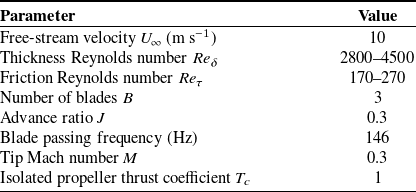
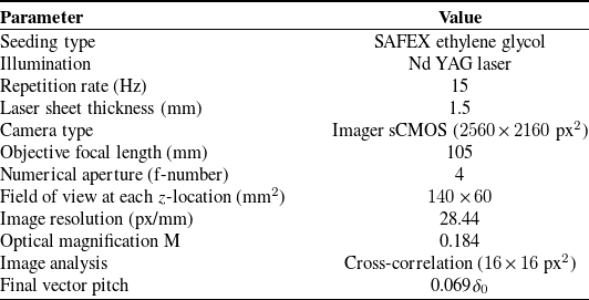


 Open access