


1. Introduction
A favourite Italian dessert is the panna cotta, similar to thick custard or blancmange. It resists the force of gravity, to stand up in the shape in which it was set, but wobbles like jelly after being lightly disturbed, quickly returning to its original configuration. Then, when the spoon is pushed in, the panna cotta smoothly and irrevocably flows apart along a seam. The material therefore combines the properties of a deformable or soft, viscoelastic solid, with those of a viscous fluid, depending on the strength of the imposed stress. In other words, panna cotta has properties one usually associates with a yield-stress fluid. A great many other materials share these properties, from mud and lava in geophysical contexts, to mucus in biology and to creams, gels and slurries in industrial processes. The flows associated with these materials have application in a wide and colourful variety of settings, ranging from geological hazards, to locomotion and to transport, mixing and optimisation problems.
Solid mechanicians typically view the yield stress from below, considering the recoverable displacements arising before flow, and determining when yield occurs as a mode of failure. Fluid mechanicians often consider the yield stress as a nuisance, complicating the effective viscosity of the material and rendering it singular as yield is approached from above. Plasticity theory applies in between, with classical approaches sometimes ignoring any solid-like deformation below the yield point or viscous effects above it. Unsurprisingly, however, the true nature of a material like panna cotta can only by appreciated by fully understanding the transition from the viscoelastic solid below the yield stress to the viscoplastic fluid above it. We refer the reader to recent reviews for a fuller discussion on such issues and more (Balmforth, Frigaard & Ovarlez Reference Balmforth, Frigaard and Ovarlez2014; Bonn et al. Reference Bonn, Denn, Berthier, Divoux and Manneville2017; Coussot Reference Coussot2018; Frigaard Reference Frigaard2019a ; Larson & Wei Reference Larson and Wei2019).
Notwithstanding this last point, here, we adopt the historical perspective of the fluid mechanician, and explore how the simple presence of a yield stress can fundamentally impact viscous flow behaviour. Throughout this work we focus on the idealised setting of relatively slow, steady flows in two spatial dimensions; this is the setting of the classical Stokes problem in viscous fluid mechanics, for which we have over a century’s worth of analysis and understanding to exploit. With a yield stress and its fundamentally nonlinear nature, however, many of the tools and much of the intuition built for Stokes flows no longer apply. Indeed, the yield stress introduces a range of new features into slow, steady flows. Our purpose here is to illustrate how the yield stress impacts flow problems, and identify the novelties. Our overarching goal is to re-establish some of the intuition lost from the Stokes problem by the incorporation of the yield stress.
For that reason, we focus most of our discussion on one of the simplest kinds of viscoplastic fluid: an incompressible material described by the Herschel–Bulkley constitutive law (which contains within it, as a limiting case, the famous Bingham plastic constitutive law; Hohenemser & Prager (Reference Hohenemser and Prager1932); Oldroyd (Reference Oldroyd1947a )). Such a material is characterised by a scalar yield stress, above which it flows in a viscous manner and below which it is rigid. Because our goal is chiefly to consider the impact of the yield stress, our interest is well away from the Newtonian limit. Indeed, we focus on situations where the yield stress is relatively strong, or equivalently, when the flow is very slow. Both translate to the ‘plastic limit’ of the problem, where the yield stress dominates the internal stresses, except over the narrow boundary layers wherein length scales are sufficiently small that viscous effects survive (Oldroyd Reference Oldroyd1947b ; Balmforth et al. Reference Balmforth, Craster, Hewitt, Hormozi and Maleki2017).
We begin in § 2 with an illustrative overview of various common dynamical features that occur in slow, steady viscoplastic flows in this plastic limit. This discussion sets the scene for the remainder of the article by conceptually introducing much of the interesting phenomenology of viscoplastic flows, the analysis and interpretation of which occupies the subsequent sections. After this opening overview section, we proceed to outline the mathematical foundations, including some details of plasticity theory, in § 3, before presenting three extended ‘case studies’ of viscoplastic problems in §§ 4, 5 and 6. These illustrate many of the features already introduced in § 2, but are considered in somewhat more detail. Conceptual issues, points of interest and open research questions are discussed throughout these sections as they arise; these ideas are all then brought together in a final discussion and perspectives section (§ 7).
2. Canonical viscoplastic behaviour: an overview
The defining feature of a viscoplastic material is the presence of a threshold yield stress; if the stress exceeds this value, the material yields and flows. The simplest models assume that the threshold value is a material constant, that the material is rigid and undeformed below the threshold, and that the rheological response of the material is always an instantaneous function of the local strain rate (thus precluding any elastic effects). Given a flow field $\boldsymbol{u}$
, the associated deviatoric stress
$\boldsymbol{u}$
, the associated deviatoric stress $\boldsymbol{\tau }$
and strain rate
$\boldsymbol{\tau }$
and strain rate $\boldsymbol{{\dot \gamma }} = \boldsymbol{\nabla u} +\boldsymbol{\nabla u}^T$
are then related by
$\boldsymbol{{\dot \gamma }} = \boldsymbol{\nabla u} +\boldsymbol{\nabla u}^T$
are then related by
 \begin{align} \boldsymbol{{\dot \gamma }} = \boldsymbol{0} \qquad & \text{for} \quad \tau \lt {\tau _{_{_P}}}, \end{align}
 \begin{align} {\boldsymbol{\tau }} = \left [\frac {{\tau _{_{_P}}}}{{\dot \gamma }} + {\mu }({\dot \gamma }) \right ] {\dot {\boldsymbol{\gamma }}} \qquad & \text{for} \quad \tau \geqslant {\tau _{_{_P}}}, \end{align}
where the symbols $\dot {\gamma }$
and
$\dot {\gamma }$
and $\tau$
refer to the scalar second invariants of the respective tensors,
$\tau$
refer to the scalar second invariants of the respective tensors, ${\dot {\gamma }} = \sqrt { (1/2){\dot \gamma }_{ij}{\dot \gamma }_{ij}}$
and
${\dot {\gamma }} = \sqrt { (1/2){\dot \gamma }_{ij}{\dot \gamma }_{ij}}$
and $\tau = \sqrt { (1/2)\tau _{ij}\tau _{ij}}$
. The yield stress is
$\tau = \sqrt { (1/2)\tau _{ij}\tau _{ij}}$
. The yield stress is $\tau _{_{_P}}$
and the function
$\tau _{_{_P}}$
and the function ${\mu }({\dot \gamma })$
here is the generalised ‘plastic’ viscosity. It is immediately clear that the stress state of the material is determined by contributions from both plastic and viscous stresses (the first and second terms in (2.2), respectively) when the yield threshold is exceeded. The relative importance of these contributions is typically measured by the ‘Bingham number’
${\mu }({\dot \gamma })$
here is the generalised ‘plastic’ viscosity. It is immediately clear that the stress state of the material is determined by contributions from both plastic and viscous stresses (the first and second terms in (2.2), respectively) when the yield threshold is exceeded. The relative importance of these contributions is typically measured by the ‘Bingham number’ $\textit{Bi}$
, which, given a flow problem with length and velocity scales
$\textit{Bi}$
, which, given a flow problem with length and velocity scales $\mathcal{L}$
and
$\mathcal{L}$
and $\mathcal{U}$
, respectively, and thus strain-rate scale
$\mathcal{U}$
, respectively, and thus strain-rate scale $\mathcal{U}/\mathcal{L}$
, is
$\mathcal{U}/\mathcal{L}$
, is
 \begin{equation} \textit{Bi} = \frac {{\tau _{_{_P}}} \mathcal{L}}{\mathcal{U} \, {\mu }(\mathcal{U}/\mathcal{L})}. \end{equation}
We refer to the limit $\textit{Bi} \gg 1$
as the ‘plastic limit’ of the problem: in this limit the yield stress plays a dominant role in the dynamics of the flow, and, as we shall see, flow solutions can look remarkably unlike their Newtonian counterparts. Note that this limit is achieved both when the yield stress itself is large, but also for arbitrary non-zero yield stress when the strain rate is sufficiently small (at the initiation of motion, for example).
$\textit{Bi} \gg 1$
as the ‘plastic limit’ of the problem: in this limit the yield stress plays a dominant role in the dynamics of the flow, and, as we shall see, flow solutions can look remarkably unlike their Newtonian counterparts. Note that this limit is achieved both when the yield stress itself is large, but also for arbitrary non-zero yield stress when the strain rate is sufficiently small (at the initiation of motion, for example).
Before delving into the mathematical and numerical details associated with manipulating and analysing constitutive laws of the kind outlined above, we first provide a brief overview of the different sorts of behaviour that such a model can produce. There are various hallmarks of viscoplastic flows when $\textit{Bi} \gg 1$
that will recur throughout this work, and these are perhaps best introduced by means of an example flow solution. Figure 1 shows sample numerical solutions of two-dimensional, inertialess flow of a Bingham fluid (
$\textit{Bi} \gg 1$
that will recur throughout this work, and these are perhaps best introduced by means of an example flow solution. Figure 1 shows sample numerical solutions of two-dimensional, inertialess flow of a Bingham fluid ( ${\mu } = \text{constant}$
in (2.2)) around a translating disk (e.g. Roquet & Saramito (Reference Roquet and Saramito2003); Tokpavi, Magnin & Jay (Reference Tokpavi, Magnin and Jay2008); Chaparian & Frigaard (Reference Chaparian and Frigaard2017b
); Supekar, Hewitt & Balmforth (Reference Supekar, Hewitt and Balmforth2020)). This problem is well known in viscous fluid mechanics as a setting for the famous Stokes paradox: there is no purely viscous solution for flow around a translating disk; inertial effects inevitably impact the flow sufficiently far from the disk. Viscoplastic fluids have no such problem: the stress must decay away from the translating disk and, for any Bingham number, will eventually ‘plug up’ the material as it falls below the yield stress (see, e.g. Hewitt & Balmforth (Reference Hewitt and Balmforth2018)). That feature is a generic one for viscoplastic problems: stresses decay away from the point(s) of disturbance, causing the material to plug up sufficiently far away. As the influence of the yield stress (i.e.
${\mu } = \text{constant}$
in (2.2)) around a translating disk (e.g. Roquet & Saramito (Reference Roquet and Saramito2003); Tokpavi, Magnin & Jay (Reference Tokpavi, Magnin and Jay2008); Chaparian & Frigaard (Reference Chaparian and Frigaard2017b
); Supekar, Hewitt & Balmforth (Reference Supekar, Hewitt and Balmforth2020)). This problem is well known in viscous fluid mechanics as a setting for the famous Stokes paradox: there is no purely viscous solution for flow around a translating disk; inertial effects inevitably impact the flow sufficiently far from the disk. Viscoplastic fluids have no such problem: the stress must decay away from the translating disk and, for any Bingham number, will eventually ‘plug up’ the material as it falls below the yield stress (see, e.g. Hewitt & Balmforth (Reference Hewitt and Balmforth2018)). That feature is a generic one for viscoplastic problems: stresses decay away from the point(s) of disturbance, causing the material to plug up sufficiently far away. As the influence of the yield stress (i.e. $\textit{Bi}$
) is increased, the yielded region of deformation typically becomes increasingly localised to the source of the disturbance.
$\textit{Bi}$
) is increased, the yielded region of deformation typically becomes increasingly localised to the source of the disturbance.
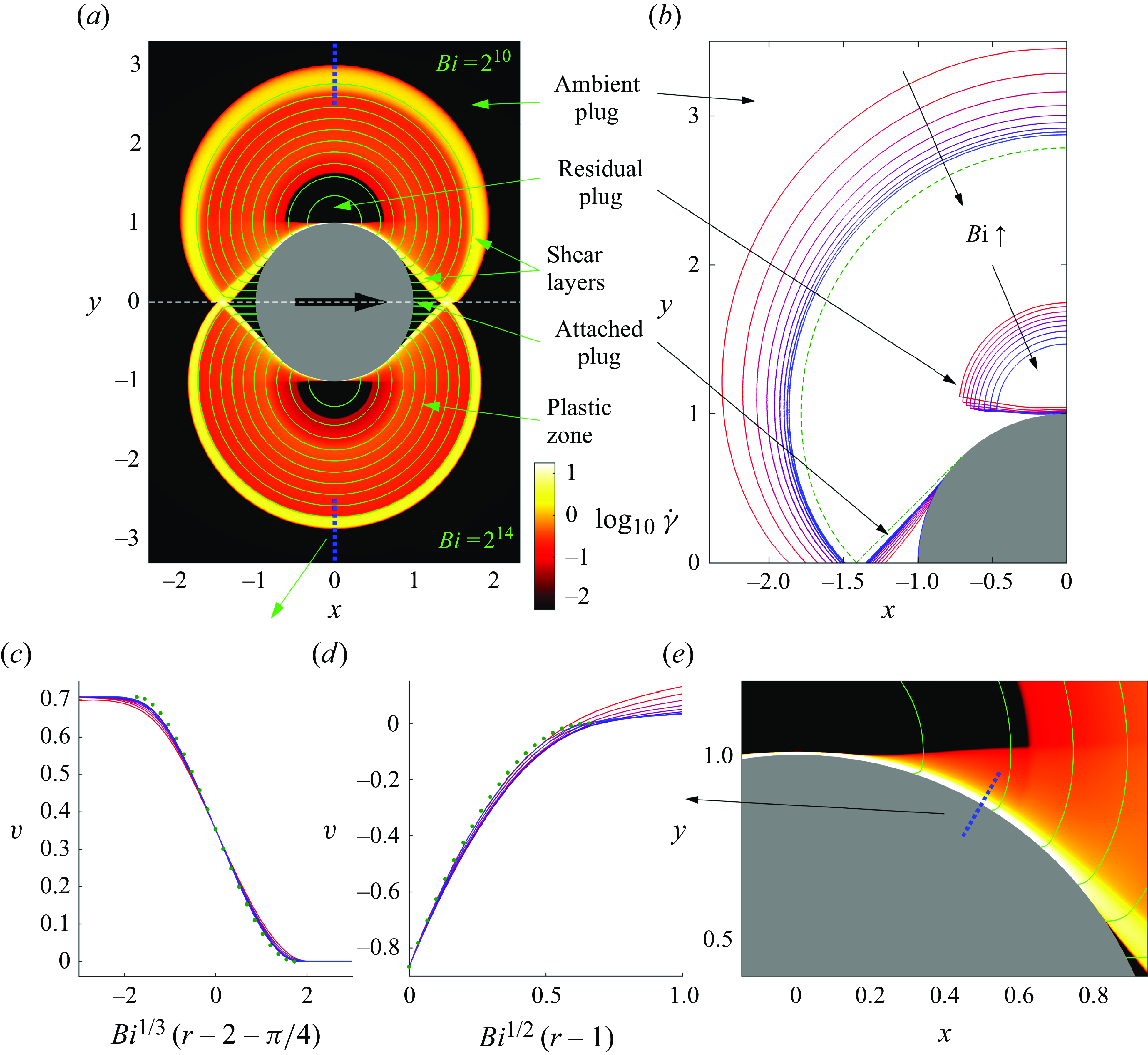
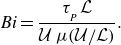
Figure 1. (a) Numerical solution for the nearly plastic flow of a Bingham fluid around a disk translating to the right. Shown is the logarithmic shear rate $\log _{10}{\dot \gamma }$
as a density map over the
$\log _{10}{\dot \gamma }$
as a density map over the $(x,y)$
-plane, for two solutions with different values for the dimensionless yield stress (
$(x,y)$
-plane, for two solutions with different values for the dimensionless yield stress ( $\textit{Bi}=2^{10}$
, top;
$\textit{Bi}=2^{10}$
, top; $2^{14}$
, bottom; each full solution is symmetric about
$2^{14}$
, bottom; each full solution is symmetric about $y=0$
). The green lines show a selection of streamlines. In (b) the borders of the plugs are shown for a wider suite of computed solutions with
$y=0$
). The green lines show a selection of streamlines. In (b) the borders of the plugs are shown for a wider suite of computed solutions with $\textit{Bi}=2^j$
,
$\textit{Bi}=2^j$
, $j=6,7,\ldots, 16$
, with yield stress increasing as indicated (and colour coded from red to blue). The (green) dashed and dot-dashed lines indicate the outer yield surface and border of the serendipitous plug of the perfectly plastic solution (Randolph & Houlsby Reference Randolph and Houlsby1984). The wall boundary layer along the top side of the disk for
$j=6,7,\ldots, 16$
, with yield stress increasing as indicated (and colour coded from red to blue). The (green) dashed and dot-dashed lines indicate the outer yield surface and border of the serendipitous plug of the perfectly plastic solution (Randolph & Houlsby Reference Randolph and Houlsby1984). The wall boundary layer along the top side of the disk for $\textit{Bi}=2^{10}=1024$
is shown in more detail in (d). Angular velocity
$\textit{Bi}=2^{10}=1024$
is shown in more detail in (d). Angular velocity $v$
profiles are plotted in (c,d) along the cuts indicated by dotted blue lines in (a) and (e), for the suite of computations in (b). These profiles are collapsed by plotting
$v$
profiles are plotted in (c,d) along the cuts indicated by dotted blue lines in (a) and (e), for the suite of computations in (b). These profiles are collapsed by plotting $v$
against the scaled coordinates indicated, and compared with the predictions of boundary-layer theory (green dots; §§ C.1.1 and C.1.2).
$v$
against the scaled coordinates indicated, and compared with the predictions of boundary-layer theory (green dots; §§ C.1.1 and C.1.2).
That said, as seen in figure 1(a), which shows the deformation-rate field for two different values of $\textit{Bi} \gg 1$
separated by roughly an order of magnitude, the flow pattern is richer than just a simple localisation of viscous motion. Moreover, flow does not become confined to narrow regions around the disk. In fact, the region of yielded material in the two cases is almost identical, indicating that the flow field converges towards a non-trivial plastic limit as
$\textit{Bi} \gg 1$
separated by roughly an order of magnitude, the flow pattern is richer than just a simple localisation of viscous motion. Moreover, flow does not become confined to narrow regions around the disk. In fact, the region of yielded material in the two cases is almost identical, indicating that the flow field converges towards a non-trivial plastic limit as $\textit{Bi} \to \infty$
. The colour map and logarithmic scale used here helpfully illustrate both the location of the rigid plugs (black) and the relative contributions of plastic deformations (small, but non-zero strain rates; orange) and residual viscous motion (larger strain rates; yellow). The anatomy of these solutions reflects an interplay between the extended plastic regions, thin viscous layers and unyielded plugs.
$\textit{Bi} \to \infty$
. The colour map and logarithmic scale used here helpfully illustrate both the location of the rigid plugs (black) and the relative contributions of plastic deformations (small, but non-zero strain rates; orange) and residual viscous motion (larger strain rates; yellow). The anatomy of these solutions reflects an interplay between the extended plastic regions, thin viscous layers and unyielded plugs.
The extended regions of nearly plastic deformation dominate the flow pattern when $\textit{Bi} \gg 1$
. In figure 1(a), these regions extend out to circular arcs beginning from a point ahead of the disk to a (symmetric) point at the back; fluid circulates from fore to aft within them. Small, rigidly rotating plugs occupy the centres of the circulating flows, while narrow shear layers act as buffers from both the outer unyielded plug and from the moving disk. Two other, rigidly translating plugs with triangular yield surfaces are attached to the disk at the front and back. The stress and deformation fields in the extended regions of nearly plastic deformation approach those for a disk moving in a perfectly plastic material (Randolph & Houlsby Reference Randolph and Houlsby1984); the clean, geometrical nature of these regions reflects an underlying map of characteristics, the so-called slipline field (Hill Reference Hill1950; Prager & Hodge Reference Prager and Hodge1951), that solve the hyperbolic plastic problem, as discussed in more detail in § 3.4 below.
$\textit{Bi} \gg 1$
. In figure 1(a), these regions extend out to circular arcs beginning from a point ahead of the disk to a (symmetric) point at the back; fluid circulates from fore to aft within them. Small, rigidly rotating plugs occupy the centres of the circulating flows, while narrow shear layers act as buffers from both the outer unyielded plug and from the moving disk. Two other, rigidly translating plugs with triangular yield surfaces are attached to the disk at the front and back. The stress and deformation fields in the extended regions of nearly plastic deformation approach those for a disk moving in a perfectly plastic material (Randolph & Houlsby Reference Randolph and Houlsby1984); the clean, geometrical nature of these regions reflects an underlying map of characteristics, the so-called slipline field (Hill Reference Hill1950; Prager & Hodge Reference Prager and Hodge1951), that solve the hyperbolic plastic problem, as discussed in more detail in § 3.4 below.
Over the shear layers that buffer the extended nearly plastic regions, viscous stresses become important, and their interplay with the plastic stresses controls the dynamics (see Oldroyd (Reference Oldroyd1947b
); Balmforth et al. (Reference Balmforth, Craster, Hewitt, Hormozi and Maleki2017)). It turns out, however, that the nature of this control depends on whether one boundary is a rigid wall or not (in essence, there is a fixed constraint on the magnitude of the stress at the edge of a plug region that is absent if the layer borders a rigid wall). As demonstrated in detail in Appendix C, wall-bounded layers are generically thinner, with higher shear rates, than ‘free’ shear layers bordering a plug. In figure 1, panels (c) and (d) show how the widths of these two types of boundary layers scale with $\textit{Bi}^{-1/2}$
and
$\textit{Bi}^{-1/2}$
and $\textit{Bi}^{-1/3}$
, respectively. Those scalings, in each case, follow from consideration of the size of the pressure drop across the layers. These viscoplastic layers have vanishing thickness for
$\textit{Bi}^{-1/3}$
, respectively. Those scalings, in each case, follow from consideration of the size of the pressure drop across the layers. These viscoplastic layers have vanishing thickness for $\textit{Bi}\to \infty$
, becoming lines of slip in the perfectly plastic limit.
$\textit{Bi}\to \infty$
, becoming lines of slip in the perfectly plastic limit.
Finally, the plugs also come in different varieties. The outer, ‘ambient’ plug of figure 1 is one variety, corresponding to a permanent feature of the plastic limit. This permanence is visible in panel (b), which plots the yield surfaces for computations with varying $\textit{Bi}$
. The outermost yield surface, the border of the ambient plug, converges to a finite curve for
$\textit{Bi}$
. The outermost yield surface, the border of the ambient plug, converges to a finite curve for $\textit{Bi}\to \infty$
which corresponds to the yield surface of the perfectly plastic slipline solution (Randolph & Houlsby Reference Randolph and Houlsby1984). In addition to appearing in the perfectly plastic solution, these ‘permanent’ plugs are characterised by stress fields that certainly fall below the yield value.
$\textit{Bi}\to \infty$
which corresponds to the yield surface of the perfectly plastic slipline solution (Randolph & Houlsby Reference Randolph and Houlsby1984). In addition to appearing in the perfectly plastic solution, these ‘permanent’ plugs are characterised by stress fields that certainly fall below the yield value.
A second plug variety is illustrated by the rotating plugs at the cores of the recirculation zones. Unlike the permanent plugs, these regions of rigid rotation steadily shrink as $\textit{Bi}$
is increased, and vanish completely in the limit
$\textit{Bi}$
is increased, and vanish completely in the limit $\textit{Bi} \to \infty$
(although their decay is extremely weak; Supekar et al. (Reference Supekar, Hewitt and Balmforth2020) argue that the plug radius decays like
$\textit{Bi} \to \infty$
(although their decay is extremely weak; Supekar et al. (Reference Supekar, Hewitt and Balmforth2020) argue that the plug radius decays like $\textit{Bi}^{-3/28}$
). The rotating plugs also do not feature in the perfectly plastic slipline solution. In other words, these ‘residual plugs’ constitute a second variety of plugs that have their origin in viscous effects (which are evidently sufficient to reduce stresses below the yield value for finite
$\textit{Bi}^{-3/28}$
). The rotating plugs also do not feature in the perfectly plastic slipline solution. In other words, these ‘residual plugs’ constitute a second variety of plugs that have their origin in viscous effects (which are evidently sufficient to reduce stresses below the yield value for finite $\textit{Bi}$
if the local strain rate remains relatively small).
$\textit{Bi}$
if the local strain rate remains relatively small).
Last, the rigid plugs attached to the front and back of the disk are examples of a third plug variety. In the numerical solutions, these plugs have yield surfaces that again converge to finite curves (figure 1 b), as for the permanent plugs. However, unlike the latter, the whole interior of the triangular plugs are held close to the yield threshold. Moreover, these regions are identified as part of the deforming region in the perfectly plastic solution (which we illustrate more fully below in § 5). By pure coincidence, it turns out that the velocity field over the triangular regions is simultaneously consistent with rigid-body motion, being simply an extension of the disk’s velocity. Those regions thereby become identified numerically as plugs. In fact, when we consider some other disk-flow problems in § 5, we uncover different examples in which triangular regions at the front and back truly yield and deform plastically, owing to the imposition of different velocity boundary conditions on the disk surface that lead to a conflict with rigid-body motion. The attached plugs in figure 1 are therefore examples of what one might call ‘serendipitous’ plugs.
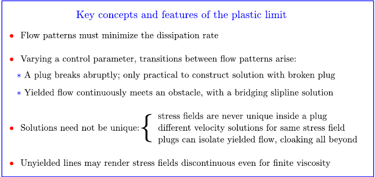
A summary of all these features, amounting to a list of expectations for the flow patterns in the plastic limit, is given in table 1. A number of principles underlie these features. These principles, and some of their consequences, will be identified and discussed in the remainder of this article, and are summarised in table 2.
Table 1. Typical flow features in the plastic limit.

Table 2. Key guiding principles underlying the typical flow features listed in table 1.
3. Mathematical foundations
3.1. Conservation laws; prototypical viscoplastic rheology
Consider the flow of a two-dimensional, incompressible, complex fluid, describing the geometry by a Cartesian coordinate system $({\hat {x}},{\hat {y}})$
. The fluid velocity is
$({\hat {x}},{\hat {y}})$
. The fluid velocity is $\boldsymbol{{\hat {u}}} = ({\hat {u}},{\hat {v}})$
. Conservation of mass and momentum demand that
$\boldsymbol{{\hat {u}}} = ({\hat {u}},{\hat {v}})$
. Conservation of mass and momentum demand that
 \begin{equation} \boldsymbol{\nabla \cdot {\hat {u}}} = 0, \end{equation}
and
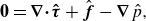 \begin{equation} \boldsymbol{0} = \boldsymbol{ \nabla \cdot } \boldsymbol{{\hat {\tau }}} + \hat {\boldsymbol{f}} - \boldsymbol{\nabla } {\hat {p}}, \end{equation}
where $\hat {p}$
is the pressure and
$\hat {p}$
is the pressure and $\hat {\boldsymbol{f}}$
represents any body force like gravity (we use the hat notation to denote dimensional variables; this decoration is removed using suitable scalings, to arrive at a dimensionless formulation, as outlined presently).
$\hat {\boldsymbol{f}}$
represents any body force like gravity (we use the hat notation to denote dimensional variables; this decoration is removed using suitable scalings, to arrive at a dimensionless formulation, as outlined presently).
One of the simplest and most popular constitutive models for a yield-stress fluid of the form of (2.2) is the Herschel-Bulkley law, with tensorial formulation
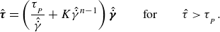 \begin{equation} \hat {\boldsymbol{\tau }} = \left (\frac {{\tau _{_{_P}}}}{\hat {\dot \gamma }} + K \hat {\dot \gamma }^{n-1} \right ) \hat {\dot {\boldsymbol{\gamma }}} \qquad \textrm {for} \qquad \hat \tau \gt {\tau _{_{_P}}}. \end{equation}
The plastic viscosity, ${\mu }(\hat {{\dot \gamma }})=K\hat {{\dot \gamma }}^{n-1}$
takes the same form as the power-law fluid, with a consistency
${\mu }(\hat {{\dot \gamma }})=K\hat {{\dot \gamma }}^{n-1}$
takes the same form as the power-law fluid, with a consistency $K$
and power-law index
$K$
and power-law index $n$
. The yield stress is
$n$
. The yield stress is $\tau _{_{_P}}$
; if
$\tau _{_{_P}}$
; if $\hat \tau \lt {\tau _{_{_P}}}$
, this threshold for yield is not breached and the deformation rates must all vanish, translating to
$\hat \tau \lt {\tau _{_{_P}}}$
, this threshold for yield is not breached and the deformation rates must all vanish, translating to $\hat {\dot \gamma }_{ij}=0$
. An important special case of (3.3) is when
$\hat {\dot \gamma }_{ij}=0$
. An important special case of (3.3) is when $n=1$
and the rate-dependent part of the stress takes the form of a constant viscous stress. This is the Bingham fluid, which is popular because of its simplicity, not its realism. Fits to data obtained in rheometers more typically generate power-law exponents
$n=1$
and the rate-dependent part of the stress takes the form of a constant viscous stress. This is the Bingham fluid, which is popular because of its simplicity, not its realism. Fits to data obtained in rheometers more typically generate power-law exponents $n\lt 1$
, although the power-law form itself is usually only a rougher representation of real fluid behaviour (Balmforth et al. Reference Balmforth, Frigaard and Ovarlez2014; Bonn et al. Reference Bonn, Denn, Berthier, Divoux and Manneville2017; Coussot Reference Coussot2018; Frigaard Reference Frigaard2019a
).
$n\lt 1$
, although the power-law form itself is usually only a rougher representation of real fluid behaviour (Balmforth et al. Reference Balmforth, Frigaard and Ovarlez2014; Bonn et al. Reference Bonn, Denn, Berthier, Divoux and Manneville2017; Coussot Reference Coussot2018; Frigaard Reference Frigaard2019a
).
Importantly, when ${\hat {\tau }}\lt {\tau _{_{_P}}}$
, no relation is imposed between the stresses and strain rates. In two dimensions, the two force-balance equations (3.2) are then insufficient to determine the two independent components of
${\hat {\tau }}\lt {\tau _{_{_P}}}$
, no relation is imposed between the stresses and strain rates. In two dimensions, the two force-balance equations (3.2) are then insufficient to determine the two independent components of $\hat {\boldsymbol \tau }$
and the pressure
$\hat {\boldsymbol \tau }$
and the pressure $\hat {p}$
. That is, the stress state is formally indeterminate over any plugged region, which is an awkward feature of the problem that will recur often in our discussion.
$\hat {p}$
. That is, the stress state is formally indeterminate over any plugged region, which is an awkward feature of the problem that will recur often in our discussion.
3.2. Scaling and dimensionless formulation
It is helpful to reformulate the equations in dimensionless form and identify key dimensionless groups. We have already identified the Bingham number (2.3) as the ratio of viscous and yield-stress scales; for the Herschel–Bulkley law, given length and velocity scales $\mathcal{L}$
and
$\mathcal{L}$
and $\mathcal{U}$
, the Bingham number is
$\mathcal{U}$
, the Bingham number is
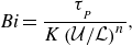 \begin{equation} \textit{Bi} = \frac {{\tau _{_{_P}}}}{K\left ({\mathcal{U}}/{\mathcal{L}}\right )^n}, \end{equation}
with $\textit{Bi} \gg 1$
denoting the plastic limit of the problem. Alternatively, when the velocity scale is not imposed, but a body force like gravity is present, a stress scale
$\textit{Bi} \gg 1$
denoting the plastic limit of the problem. Alternatively, when the velocity scale is not imposed, but a body force like gravity is present, a stress scale $\mathcal{P}$
can be defined (such as
$\mathcal{P}$
can be defined (such as $\mathcal{P} = \rho g \mathcal{L}$
). In this circumstance, one can define a velocity scale
$\mathcal{P} = \rho g \mathcal{L}$
). In this circumstance, one can define a velocity scale
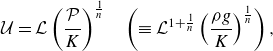 \begin{equation} \mathcal{U} = \mathcal{L} \left ( \frac {\mathcal{P}}{K} \right )^{\frac 1n} \quad \left (\equiv \mathcal{L}^{1+\frac 1n} \left ( \frac {\rho g}{K} \right )^{\frac 1n} \right ), \end{equation}
where $\rho$
and
$\rho$
and $g$
denote density and gravitational acceleration and the Bingham number in (3.4) becomes
$g$
denote density and gravitational acceleration and the Bingham number in (3.4) becomes $\textit{Bi}={\tau _{_{_P}}}/\mathcal{P}$
(or
$\textit{Bi}={\tau _{_{_P}}}/\mathcal{P}$
(or ${\tau _{_{_P}}}/(\rho g \mathcal{L})$
). This parameter must remain order one if the applied stresses are to exceed the yield stress and force motion. Strictly speaking,
${\tau _{_{_P}}}/(\rho g \mathcal{L})$
). This parameter must remain order one if the applied stresses are to exceed the yield stress and force motion. Strictly speaking, $\textit{Bi}$
now represents the ratio of yield stress to the imposed stress, and (for gravity) is sometimes referred to as the ‘Oldroyd number’ instead. The plastic limit is then characterised by the special value of
$\textit{Bi}$
now represents the ratio of yield stress to the imposed stress, and (for gravity) is sometimes referred to as the ‘Oldroyd number’ instead. The plastic limit is then characterised by the special value of $\textit{Bi}$
for which the fluid speed approaches zero. That is, the plastic limit corresponds to the threshold for motion.
$\textit{Bi}$
for which the fluid speed approaches zero. That is, the plastic limit corresponds to the threshold for motion.
For two-dimensional flow without body forces, we write the dimensionless governing equations using either a Cartesian coordinate system $(x,y)$
or general curvilinear coordinates
$(x,y)$
or general curvilinear coordinates $(s,\eta )$
built from the arc length along some prescribed curve and its normal:
$(s,\eta )$
built from the arc length along some prescribed curve and its normal:
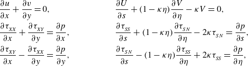 \begin{equation} \begin{aligned} &\frac {\partial {u}}{\partial {x}}+\frac {\partial {v}}{\partial {y}} = 0, \cr &\frac {\partial {{\tau _{_{\textit{XX}}}}}}{\partial {x}} + \frac {\partial {{\tau _{_{\textit{XY}}}}}}{\partial {y}} = \frac {\partial {p}}{\partial {x}},\cr &\frac {\partial {{\tau _{_{\textit{XY}}}}}}{\partial {x}} - \frac {\partial {{\tau _{_{\textit{XX}}}}}}{\partial {y}} = \frac {\partial {p}}{\partial {y}}, \end{aligned} \qquad \qquad \begin{aligned} &\frac {\partial {U}}{\partial {s}} + (1-\kappa \eta )\frac {\partial {V}}{\partial {\eta }} - \kappa V = 0, \cr &\frac {\partial {{\tau _{_{\textit{SS}}}}}}{\partial {s}} + (1-\kappa \eta )\frac {\partial {{\tau _{_{SN}}}}}{\partial {\eta }} - 2\kappa {\tau _{_{SN}}} = \frac {\partial {p}}{\partial {s}},\cr &\frac {\partial {{\tau _{_{SN}}}}}{\partial {s}} - (1-\kappa \eta )\frac {\partial {{\tau _{_{\textit{SS}}}}}}{\partial {\eta }} + 2\kappa {\tau _{_{\textit{SS}}}} = \frac {\partial {p}}{\partial {\eta }}, \end{aligned} \end{equation}
where
 \begin{equation} \kappa = \frac {\partial {\theta }}{\partial {s}}, \end{equation}
is the curvature of the prescribed curve. Here and throughout this work, capital-letter subscripts are used to identify tensor components. The velocity field in Cartesian coordinates is $(u,v)$
; the curvilinear relative is
$(u,v)$
; the curvilinear relative is $(U,V)$
. The strain-rate components are given by
$(U,V)$
. The strain-rate components are given by
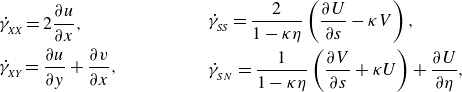 \begin{equation} \begin{aligned} &{\dot \gamma _{_{\textit{XX}}}} = 2\frac {\partial {u}}{\partial {x}},\cr &{\dot \gamma _{_{\textit{XY}}}} = \frac {\partial {u}}{\partial {y}}+\frac {\partial {v}}{\partial {x}}, \end{aligned} \qquad \qquad \begin{aligned} &{\dot \gamma _{_{\textit{SS}}}} = \frac {2}{1-\kappa \eta }\left (\frac {\partial {U}}{\partial {s}}-\kappa V\right ),\cr &{\dot \gamma _{_{SN}}} = \frac {1}{1-\kappa \eta }\left (\frac {\partial {V}}{\partial {s}}+\kappa U\right )+ \frac {\partial {U}}{\partial {\eta }}, \end{aligned} \end{equation}
and the Herschel–Bulkley constitutive law is
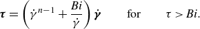 \begin{equation} \boldsymbol{\tau } = \left ({\dot \gamma }^{n-1} +\frac {\textit{Bi}}{{\dot \gamma }}\right ) \dot {\boldsymbol{\gamma }} \qquad \textrm {for} \qquad \tau \gt \textit{Bi}. \end{equation}
The nonlinear rheology in (3.9) presents some challenges for computing numerical solutions to (3.6)–(3.9), primarily because of the yield condition. A convenient, alternative approach that circumvents such challenges is provided by ‘regularising’ the constitutive law: (3.9) is replaced by a smoothed version with a well-defined and finite relationship between stress and strain rate everywhere. More precise techniques also exist, most notably the augmented Lagrangian approach, which provides an iterative solution to the exact rheology directly. Some details of both of these schemes, along with other numerical considerations and observations, are presented in Appendix A.
Alternatively, as in any fluid mechanical problem, asymptotic approaches based on an extreme difference in length scales provide a useful tool for interrogating viscoplastic flows (Balmforth Reference Balmforth2019). Shallow flows can be attacked with a generalisation of viscous lubrication theory, although the approach has been incorrectly denigrated in the past because of the fallacy of the so-called lubrication paradox (Balmforth & Craster Reference Balmforth and Craster1999; Hewitt & Balmforth Reference Hewitt and Balmforth2012). More generally, and as illustrated earlier, viscous deformation becomes restricted to narrow boundary layers in the plastic limit, which are amenable to boundary-layer analysis (Oldroyd Reference Oldroyd1947b ; Balmforth et al. Reference Balmforth, Craster, Hewitt, Hormozi and Maleki2017). Such asymptotic approaches can become technically involved; the interested reader can find further details in Appendix C.
3.3. Extremum principles and minimum dissipation
The (dimensionless) governing equations can be cast into a variational form that identifies extremum principles satisfied by the velocity and stress fields (see Prager (Reference Prager1954) and, for example, Frigaard (Reference Frigaard2019b )). We quote these principles in settings for which we ignore any body forces (i.e. gravity) and the velocity field is prescribed on all the boundaries. The principles therefore apply to the steady flow problems considered in § 4 and § 5, and provide a useful constraint associated with the net dissipation rate on the solutions in the plastic limit.
The first principle is that, of all the divergence-free velocity fields $\boldsymbol{v}$
that match up with the velocities along the boundaries, the actual velocity field
$\boldsymbol{v}$
that match up with the velocities along the boundaries, the actual velocity field $\boldsymbol{u}$
minimises the functional
$\boldsymbol{u}$
minimises the functional
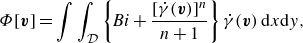 \begin{equation} \Phi [\boldsymbol{v}] = \int \int _{\mathcal{D}} \left \{ \textit{Bi} + \frac {[{\dot \gamma }(\boldsymbol{v})]^{n}}{n+1}\right \} {\dot \gamma }(\boldsymbol{v}) \; \textrm {d} x\textrm {d} y, \end{equation}
where $\mathcal{D}$
denotes the domain occupied by the fluid and
$\mathcal{D}$
denotes the domain occupied by the fluid and ${\dot \gamma }(\boldsymbol{v})$
denotes the strain-rate invariant built from
${\dot \gamma }(\boldsymbol{v})$
denotes the strain-rate invariant built from $\boldsymbol{v}$
. In this minimisation, the trial velocity fields are not linked through the constitutive law to any stress field.
$\boldsymbol{v}$
. In this minimisation, the trial velocity fields are not linked through the constitutive law to any stress field.
The second principle is that, of all the possible stress fields $\tilde {\boldsymbol{\sigma }}$
that satisfy the force-balance equations, independently of the constitutive law, the actual stress
$\tilde {\boldsymbol{\sigma }}$
that satisfy the force-balance equations, independently of the constitutive law, the actual stress $\boldsymbol{\sigma }$
maximises
$\boldsymbol{\sigma }$
maximises
 \begin{equation} \Psi [\tilde {\boldsymbol{\sigma }}] = \int _{\partial \mathcal{D}} \boldsymbol{u \cdot } \tilde {\boldsymbol{\sigma }} \boldsymbol{\cdot } \boldsymbol{\hat {n}} \; \textrm {d} s - \frac {n}{n+1} \int \int _{\mathcal{D}} \left \{ \textrm {Max}\left [0, \tau (\tilde {\boldsymbol{\sigma }}) - \textit{Bi} \right ] \right \}^{1+\frac 1n} \; \textrm {d} x\textrm {d} y, \end{equation}
where $\partial \mathcal{D}$
denotes the boundary of the fluid domain, with unit outward normal
$\partial \mathcal{D}$
denotes the boundary of the fluid domain, with unit outward normal $\boldsymbol{\hat {n}}$
and infinitesimal arc length
$\boldsymbol{\hat {n}}$
and infinitesimal arc length $\textrm {d} s$
, and
$\textrm {d} s$
, and $\tau (\tilde {\boldsymbol{\sigma }})$
denotes the second invariant of the trial stress field.
$\tau (\tilde {\boldsymbol{\sigma }})$
denotes the second invariant of the trial stress field.
Necessarily, when the extrema are achieved, we also have that $\Phi [\boldsymbol{u}]=\Psi [ \boldsymbol{\sigma }]$
, which corresponds to the integral constraint
$\Phi [\boldsymbol{u}]=\Psi [ \boldsymbol{\sigma }]$
, which corresponds to the integral constraint
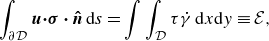 \begin{equation} \int _{\partial \mathcal{D}} \boldsymbol{u \cdot } \boldsymbol{\sigma } \boldsymbol{\cdot } \boldsymbol{\hat {n}} \; \textrm {d} s = \int \int _{\mathcal{D}} \tau {\dot \gamma } \; \textrm {d} x\textrm {d} y \equiv \mathcal{E}, \end{equation}
and is simply an expression of the fact that the power supplied through boundaries (the left-hand side) must balance the net dissipation rate ( $\mathcal{E}$
, the second integral). Importantly, in the plastic limit,
$\mathcal{E}$
, the second integral). Importantly, in the plastic limit, $\tau {\dot \gamma } \to \textit{Bi}{\dot \gamma }$
and the velocity minimisation corresponds to selecting the trial velocity field that has the least net rate of dissipation. In addition, if a body force is present (cf. § 6), the work performed by that force must also be added to the variational problems and to (3.12) (Prager Reference Prager1954; Frigaard Reference Frigaard2019b
).
$\tau {\dot \gamma } \to \textit{Bi}{\dot \gamma }$
and the velocity minimisation corresponds to selecting the trial velocity field that has the least net rate of dissipation. In addition, if a body force is present (cf. § 6), the work performed by that force must also be added to the variational problems and to (3.12) (Prager Reference Prager1954; Frigaard Reference Frigaard2019b
).
3.4. Plasticity theory
For $\textit{Bi}\gg 1$
, the theory of perfect plasticity applies (Hill Reference Hill1950; Prager & Hodge Reference Prager and Hodge1951); key concepts for generating solutions in this limit are provided below. Additional details of slipline analysis, and a sample construction of a relevant slipline pattern, can be found in Appendix B.
$\textit{Bi}\gg 1$
, the theory of perfect plasticity applies (Hill Reference Hill1950; Prager & Hodge Reference Prager and Hodge1951); key concepts for generating solutions in this limit are provided below. Additional details of slipline analysis, and a sample construction of a relevant slipline pattern, can be found in Appendix B.
3.4.1. Sliplines
In terms of our two-dimensional Cartesian coordinate system, the constitutive law in the ideal plastic limit reduces to
 \begin{equation} {\tau ^2_{_{\textit{XY}}}}+{\tau ^2_{_{\textit{XX}}}}=\textit{Bi}^2, \end{equation}
which motivates the definition of the new variable $\theta$
in
$\theta$
in
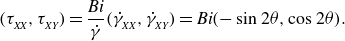 \begin{equation} ({\tau _{_{\textit{XX}}}},{\tau _{_{\textit{XY}}}}) = \frac {\textit{Bi}}{{\dot \gamma }}({\dot \gamma _{_{\textit{XX}}}},{\dot \gamma _{_{\textit{XY}}}}) = \textit{Bi}(-\sin 2\theta, \cos 2\theta ). \end{equation}
We may then manipulate the force-balance equations (3.2) into the hyperbolic pairing
 \begin{equation} \left (\frac {\partial }{\partial {y}}+\cot \theta \frac {\partial }{\partial {x}}\right )(p + 2 \textit{Bi} \theta ) = 0 \qquad \& \qquad \left (\frac {\partial }{\partial {y}}-\tan \theta \frac {\partial }{\partial {x}}\right )(p - 2 \textit{Bi} \theta ) = 0 . \end{equation}
That is, we have the Riemann invariant $p+2\textit{Bi}\theta$
along the curves with
$p+2\textit{Bi}\theta$
along the curves with $\textrm {d} y/\textrm {d} x = \tan \theta$
; the curves with
$\textrm {d} y/\textrm {d} x = \tan \theta$
; the curves with $\textrm {d} y/\textrm {d} x = -\cot \theta$
have
$\textrm {d} y/\textrm {d} x = -\cot \theta$
have $p-2\textit{Bi}\theta = \textrm{constant}$
. These characteristic curves are the ‘sliplines’ of classical plasticity theory (Hill Reference Hill1950; Prager & Hodge Reference Prager and Hodge1951). Evidently, the two sets of curves are orthogonal to one another, and are commonly referred to as the
$p-2\textit{Bi}\theta = \textrm{constant}$
. These characteristic curves are the ‘sliplines’ of classical plasticity theory (Hill Reference Hill1950; Prager & Hodge Reference Prager and Hodge1951). Evidently, the two sets of curves are orthogonal to one another, and are commonly referred to as the $\alpha$
and
$\alpha$
and $\beta $
-lines. Convention takes the two sliplines to form a local right-handed coordinate system.
$\beta $
-lines. Convention takes the two sliplines to form a local right-handed coordinate system.
The sliplines form a net that spans all the yielded regions (two examples are shown in figure 2). A number of properties of the network follow from (3.15). Two, in particular, are often quoted and termed ‘Hencky’s rules’; we describe these more thoroughly in Appendix B.1. One important consequence of them is that when a slipline of one family (i.e. $\alpha$
or
$\alpha$
or $\beta$
) is straight, then all the other lines of the same family must also be straight if sliplines from the other slipline family connect them together. This relatively strong geometrical constraint impacts the structure of the yielded regions and provides a pathway to solving the slipline equations analytically in some problems. In particular, it implies that when one slipline is straight, the acceptable slipline fields include square checkerboards and centred circular fans, as illustrated in figure 2(b), or a set of involutes to a curve such as a circle (as we encounter later).
$\beta$
) is straight, then all the other lines of the same family must also be straight if sliplines from the other slipline family connect them together. This relatively strong geometrical constraint impacts the structure of the yielded regions and provides a pathway to solving the slipline equations analytically in some problems. In particular, it implies that when one slipline is straight, the acceptable slipline fields include square checkerboards and centred circular fans, as illustrated in figure 2(b), or a set of involutes to a curve such as a circle (as we encounter later).
In general, however, the utility of sliplines is limited because rigid plugs can be present, over which (3.13) no longer holds, and any slipline can be taken to be a yield surface bounding these plugs (Hill (Reference Hill1950); Prager & Hodge (Reference Prager and Hodge1951); see also figure 2). Worse, discontinuities can also appear in the stress field. The sliplines do not remain continuous across these features, implying scars can disfigure the slipline pattern. The (total) normal and shear stresses remain continuous across any such discontinuity, but there can be a jump in the tangential normal stress (i.e. ${\sigma _{_{\textit{SS}}}}={\tau _{_{\textit{SS}}}}-p$
, if the curvilinear coordinate system is aligned with the discontinuity). These conditions translate to the requirement that the sliplines meet the discontinuity at equal angles.
${\sigma _{_{\textit{SS}}}}={\tau _{_{\textit{SS}}}}-p$
, if the curvilinear coordinate system is aligned with the discontinuity). These conditions translate to the requirement that the sliplines meet the discontinuity at equal angles.
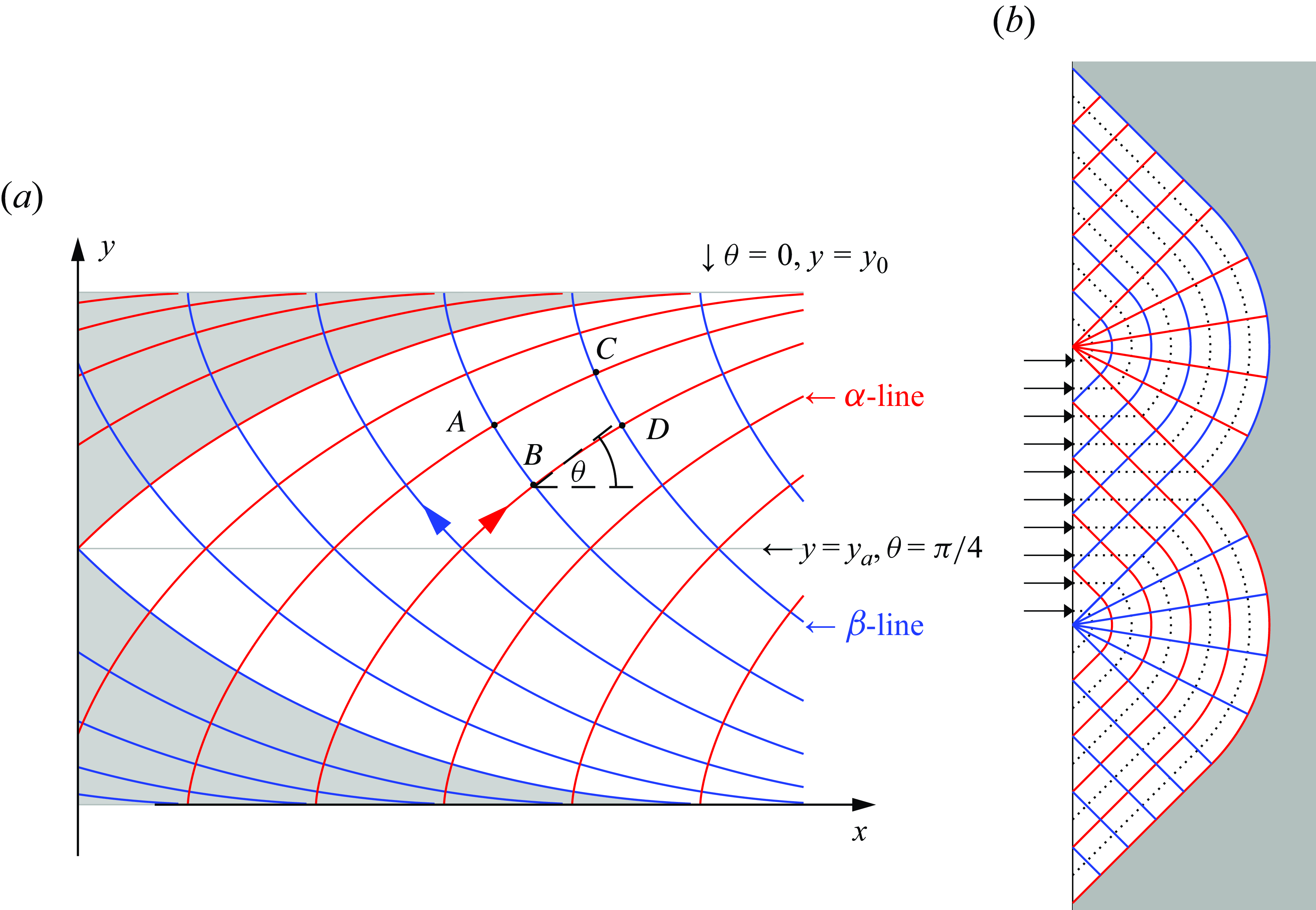
Figure 2. Illustrations of the slipline field, and Prandtl’s (a) cycloid and (b) punch solutions. The shaded regions indicate plugs. In (b), the dotted lines show sample streamlines.
Complicating matters further is that, in many problems, boundary conditions are provided on the velocity, not the stress. One cannot then construct the slipline field without a consideration of the velocity field. The components of the velocity field along the sliplines, $(v_\alpha, v_\beta )$
, satisfy the so-called Geiringer equations
$(v_\alpha, v_\beta )$
, satisfy the so-called Geiringer equations
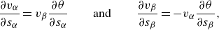 \begin{equation} \frac {\partial {v_\alpha }}{\partial {s_\alpha }}=v_\beta \frac {\partial {\theta }}{\partial {s_\alpha }} \qquad \text{and} \qquad \frac {\partial {v_\beta }}{\partial {s_\beta }}=-v_\alpha \frac {\partial {\theta }}{\partial {s_\beta }}, \end{equation}
which follow from the constraint of incompressibility (3.1). These equations imply that the plastic flow lines (i.e. the characteristics of the velocity field) coincide with the sliplines. Therefore, if the velocity field is directed along one set of sliplines, these curves also correspond to streamlines and the velocity along them remains fixed. Again, a complication is that the ideal plastic velocity field need not remain continuous. In fact, as implied by the name, a slipline can be taken as the locus of a jump in tangential velocity. In other words, velocity discontinuities can be present, but they are aligned with sliplines. Figure 2(b) also plots a selection of streamlines, corresponding to the slipline field shown. Here, fluid enters the domain at an angle to the $45^\circ$
checkerboard of sliplines. Once fluid reaches the fan, however, slip occurs, allowing the velocity to re-align with the circular arcs of the fan. Thereafter, one of the slipline families corresponds to streamlines.
$45^\circ$
checkerboard of sliplines. Once fluid reaches the fan, however, slip occurs, allowing the velocity to re-align with the circular arcs of the fan. Thereafter, one of the slipline families corresponds to streamlines.
Although the slipline field can be used to directly construct a range of perfectly plastic solutions, the difficulties implicit in the construction can make such an approach unwieldy and it is often not possible to proceed analytically. While techniques have been developed to ease numerical constructions of the slipline field (Collins Reference Collins1982), our perspective here is different. With the advent of augmented Lagrangian numerical techniques, one can solve two-dimensional problems of viscoplastic steady flow with relative ease, even close to the plastic limit. This circumvents any need to construct numerical slipline fields directly. Instead, with a numerical viscoplastic solution in hand, the slipline analysis provides a convenient tool to diagnose the solution structure, pointing to the existence of any analytical special cases and providing a means to verify the fidelity of computations. We illustrate these ideas later, using some specific flow configurations.
3.4.2. Exact solutions and constructions
Two classical exact solutions to the slipline problem date back to Prandtl and are illustrated in figure 2. The solution illustrated in figure 2(b) consists of a patchwork of circular fans and triangular checkerboards. The rightmost sliplines (a $\beta $
-line for the bottom half, and an
$\beta $
-line for the bottom half, and an $\alpha $
-line for the top) provide a yield surface. This construction was offered by Prandtl as a slipline solution for plastic indentation, following along the lines of traditional developments for the indentation of a punch in linear elasticity. Prandtl’s solution (rotated by ninety degrees) is commonly used in soil mechanics for the failure of a foundation above a cohesive soil.
$\alpha $
-line for the top) provide a yield surface. This construction was offered by Prandtl as a slipline solution for plastic indentation, following along the lines of traditional developments for the indentation of a punch in linear elasticity. Prandtl’s solution (rotated by ninety degrees) is commonly used in soil mechanics for the failure of a foundation above a cohesive soil.
A second solution offered by Prandtl applies to the compression of a plastic layer, or a squeeze flow. In this case the sliplines are cycloids: if $\theta =\theta (y)$
and
$\theta =\theta (y)$
and $p=\textit{Bi}[ -\Gamma x + \Phi (y)]$
, then the force-balance equations reduce to
$p=\textit{Bi}[ -\Gamma x + \Phi (y)]$
, then the force-balance equations reduce to
 \begin{equation} \frac{\partial}{\partial y} (\cos 2\theta) = -\Gamma \quad \& \quad \frac{\partial}{\partial y} ( \Phi + \sin 2 \theta) = 0, \end{equation}
If $\theta =0$
at
$\theta =0$
at $y=y_0$
and
$y=y_0$
and $\theta = (1/4)\pi$
at
$\theta = (1/4)\pi$
at $y=y_a$
, then the
$y=y_a$
, then the $\alpha $
-lines follow from
$\alpha $
-lines follow from
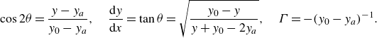 \begin{equation} \cos 2\theta = \frac {y-y_a}{y_0-y_a}, \quad \frac {\textrm {d} y}{\textrm {d} x} = \tan \theta = \sqrt {\frac {y_0-y}{y+y_0-2y_a}}, \quad \Gamma = -(y_0-y_a)^{-1}. \end{equation}
Hence
 \begin{equation} 2\tan ^{-1} \sqrt {\frac {2}{v}-1} - \sqrt {v(2-v)} + 1 - \frac {1}{2}\pi = \frac {x_0-x}{y_0-y_a}, \quad v=\frac {y_0-y}{y_0-y_a}, \end{equation}
if $x=x_0$
for
$x=x_0$
for $y=y_a$
, which is the equation for a cycloid. Note that this curve is scale free, in the sense that any scaling of
$y=y_a$
, which is the equation for a cycloid. Note that this curve is scale free, in the sense that any scaling of $y$
and
$y$
and $x$
leaves the equation unchanged (as long as
$x$
leaves the equation unchanged (as long as $\Gamma$
can be scaled suitably too). The resulting slipline field is actually what is illustrated in figure 2(a).
$\Gamma$
can be scaled suitably too). The resulting slipline field is actually what is illustrated in figure 2(a).
Note that Prandtl’s two solutions illustrate an important feature of the plasticity problem: the squeezing walls generating the cycloid solutions in figure 2(a) are assumed to be ‘fully rough’, a condition demands that the fluid slides along the wall with a local shear stress that equals the yield stress. For a viscoplastic fluid, such slip prompts the appearance of a thin wall boundary layer over which the tangential velocity is brought back to zero. In other words, fully rough boundary conditions on the walls translate to no slip, and the slipline angle is either $\theta =0$
or
$\theta =0$
or $\theta =(1/2)\pi$
. Conversely, the surface on the left in figure 2(b) is free, implying that the shear stress must vanish, and
$\theta =(1/2)\pi$
. Conversely, the surface on the left in figure 2(b) is free, implying that the shear stress must vanish, and $\theta =\pm (1/4)\pi$
. Such a condition on the slipline angle also applies along lines of symmetry, such as the midline between the squeezing plates in figure 2(b). The
$\theta =\pm (1/4)\pi$
. Such a condition on the slipline angle also applies along lines of symmetry, such as the midline between the squeezing plates in figure 2(b). The $y$
-axis can further be taken as another line of symmetry at the centre of the squeeze flow, if the shaded region is assumed to plug up with yield surfaces along the bordering sliplines. The correspondence between no-slip or free-slip boundary conditions and the fixing of the slipline angle recurs in the examples we present below.
$y$
-axis can further be taken as another line of symmetry at the centre of the squeeze flow, if the shaded region is assumed to plug up with yield surfaces along the bordering sliplines. The correspondence between no-slip or free-slip boundary conditions and the fixing of the slipline angle recurs in the examples we present below.
More generally, the slipline equations (when expressed in terms of the two local radii of curvature, or some other geometrical variables; Appendix B.1) and Geiringer’s equations reduce to the telegraph equation under a change of independent variables (from arc length to an angle parameterisation; Hill (Reference Hill1950)). Classical solutions to that problem then allow one to write down exact solutions to the plasticity problem in terms of single integrals if information is provided along a known slipline. Even if such information is not provided, one can still use this solution as the basis of a numerical scheme (Dewhurst & Collins Reference Dewhurst and Collins1973; Collins Reference Collins1982). This strategy significantly expanded the library of slipline solutions available in the plasticity literature (e.g. Collins (Reference Collins1970, Reference Collins1982)), a resource that largely remains untapped in analyses of viscoplastic fluid flows near the plastic limit. In fact, this technique leads to semi-analytical solutions, one of which is closely related to the slipline problem discussed in § 4 (Hill Reference Hill1950; Chakrabarty Reference Chakrabarty1979). Other exact solutions or constructions follow from searching for self-similar solutions (e.g. Taylor-West & Hogg (Reference Taylor-West and Hogg2021, Reference Taylor-West and Hogg2023)).
4. Jet-like intrusion
To illustrate viscoplastic flow dynamics near the plastic limit, we consider three model problems for a Bingham fluid ( $n=1$
). The first, sketched in figure 3, corresponds to a modification of a problem suggested by Oldroyd (Reference Oldroyd1947b
) in which a jet-like intrusion of viscoplastic fluid flows through a rectangular channel. The fluid enters with fixed speed
$n=1$
). The first, sketched in figure 3, corresponds to a modification of a problem suggested by Oldroyd (Reference Oldroyd1947b
) in which a jet-like intrusion of viscoplastic fluid flows through a rectangular channel. The fluid enters with fixed speed $U$
over an orifice on the left wall of width
$U$
over an orifice on the left wall of width $y_i$
, then leaves through a similar exit on the right wall. We take
$y_i$
, then leaves through a similar exit on the right wall. We take $\mathcal{L}=y_i$
as the characteristic length scale, and impose symmetry conditions along the midlines of the rectangle, at
$\mathcal{L}=y_i$
as the characteristic length scale, and impose symmetry conditions along the midlines of the rectangle, at $x=\ell _x$
and
$x=\ell _x$
and $y=0$
, reducing our computational domain to the upper left quadrant. We consider two possible boundary conditions for the walls at
$y=0$
, reducing our computational domain to the upper left quadrant. We consider two possible boundary conditions for the walls at $y=\pm \ell _y$
: no slip conditions and free slip conditions. Adopting no slip simulates flow through a localised expansion. Such flows have previously been used as model problems for viscoplastic computations (Mitsoulis & Tsamopoulos Reference Mitsoulis and Tsamopoulos2017) and experiments (Coussot Reference Coussot2014), and have received attention in the classical plasticity literature (Hill Reference Hill1950). Alternatively, with free-slip conditions, we simulate an array of vertically stacked, periodic injections. It proves useful to consider both no slip and free slip at
$y=\pm \ell _y$
: no slip conditions and free slip conditions. Adopting no slip simulates flow through a localised expansion. Such flows have previously been used as model problems for viscoplastic computations (Mitsoulis & Tsamopoulos Reference Mitsoulis and Tsamopoulos2017) and experiments (Coussot Reference Coussot2014), and have received attention in the classical plasticity literature (Hill Reference Hill1950). Alternatively, with free-slip conditions, we simulate an array of vertically stacked, periodic injections. It proves useful to consider both no slip and free slip at $y=\pm \ell _y$
in order to illustrate some important repercussions of placing a plug against a wall.
$y=\pm \ell _y$
in order to illustrate some important repercussions of placing a plug against a wall.
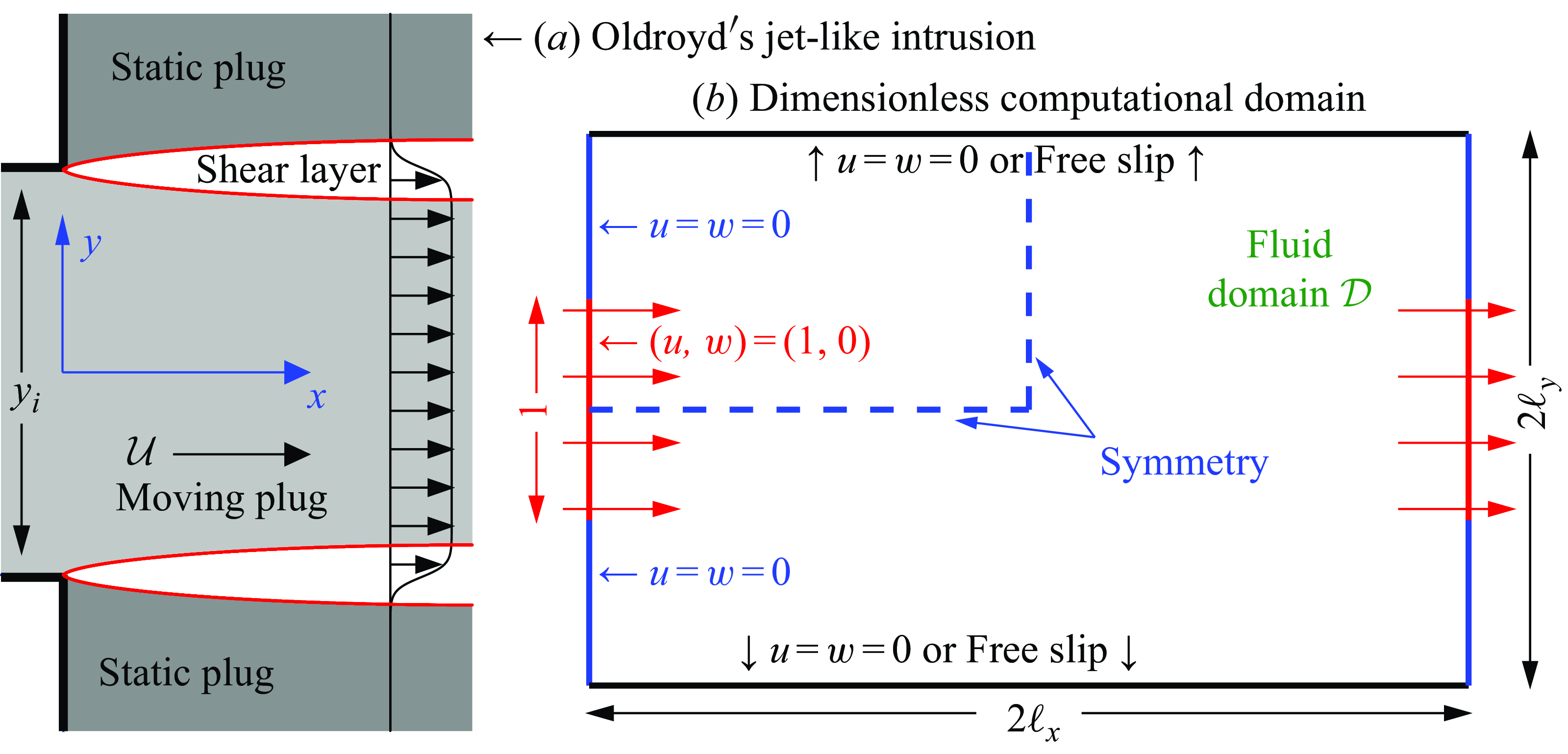
Figure 3. Sketch of a jet-like intrusion through a rectangular domain. The characteristic scales $\mathcal{L}$
and
$\mathcal{L}$
and $\mathcal{U}$
are taken to be the inflow speed
$\mathcal{U}$
are taken to be the inflow speed $U$
and the inlet width
$U$
and the inlet width $y_i$
. Practically, the symmetries about
$y_i$
. Practically, the symmetries about $y=0$
and
$y=0$
and $x=\ell_x$
are used to consider only a quarter of the domain.
$x=\ell_x$
are used to consider only a quarter of the domain.
4.1. Narrow domains; breaking the incoming plug
A suite of numerical solutions for the jet problem are displayed in figure 4. Here, the Bingham number is fixed close to the plastic limit ( $\textit{Bi}=2048$
), the cross-stream height is set at
$\textit{Bi}=2048$
), the cross-stream height is set at $\ell _y= 3/2$
and the downstream length
$\ell _y= 3/2$
and the downstream length $\ell _x$
is varied. For small domain lengths
$\ell _x$
is varied. For small domain lengths $\ell _x$
, flow enters and exits the domain as a moving plug of almost uniform width bordered by two thin shear layers (figure 4
c). This localisation of fluid deformation by the yield stress, and the creation of extensive blockages, is rather different from traditional Stokes flow, for which fluid deforms throughout the domain (and is equivalent to the localisation of viscoplastic flow around the disk in figure 1). The shear layers have a structure that can be predicted by Oldroyd’s boundary-layer theory (see figure 5
a,c), as outlined in § C.1.1. That analysis indicates that the net dissipation
$\ell _x$
, flow enters and exits the domain as a moving plug of almost uniform width bordered by two thin shear layers (figure 4
c). This localisation of fluid deformation by the yield stress, and the creation of extensive blockages, is rather different from traditional Stokes flow, for which fluid deforms throughout the domain (and is equivalent to the localisation of viscoplastic flow around the disk in figure 1). The shear layers have a structure that can be predicted by Oldroyd’s boundary-layer theory (see figure 5
a,c), as outlined in § C.1.1. That analysis indicates that the net dissipation $\mathcal{E}$
over the upper half of the domain is approximately
$\mathcal{E}$
over the upper half of the domain is approximately $\ell _x\textit{Bi}$
(cf. (C9)) and the area of the corresponding yielded region is given by (C8); both diagnostics are plotted in figure 4(a,b) for the full series of computations.
$\ell _x\textit{Bi}$
(cf. (C9)) and the area of the corresponding yielded region is given by (C8); both diagnostics are plotted in figure 4(a,b) for the full series of computations.
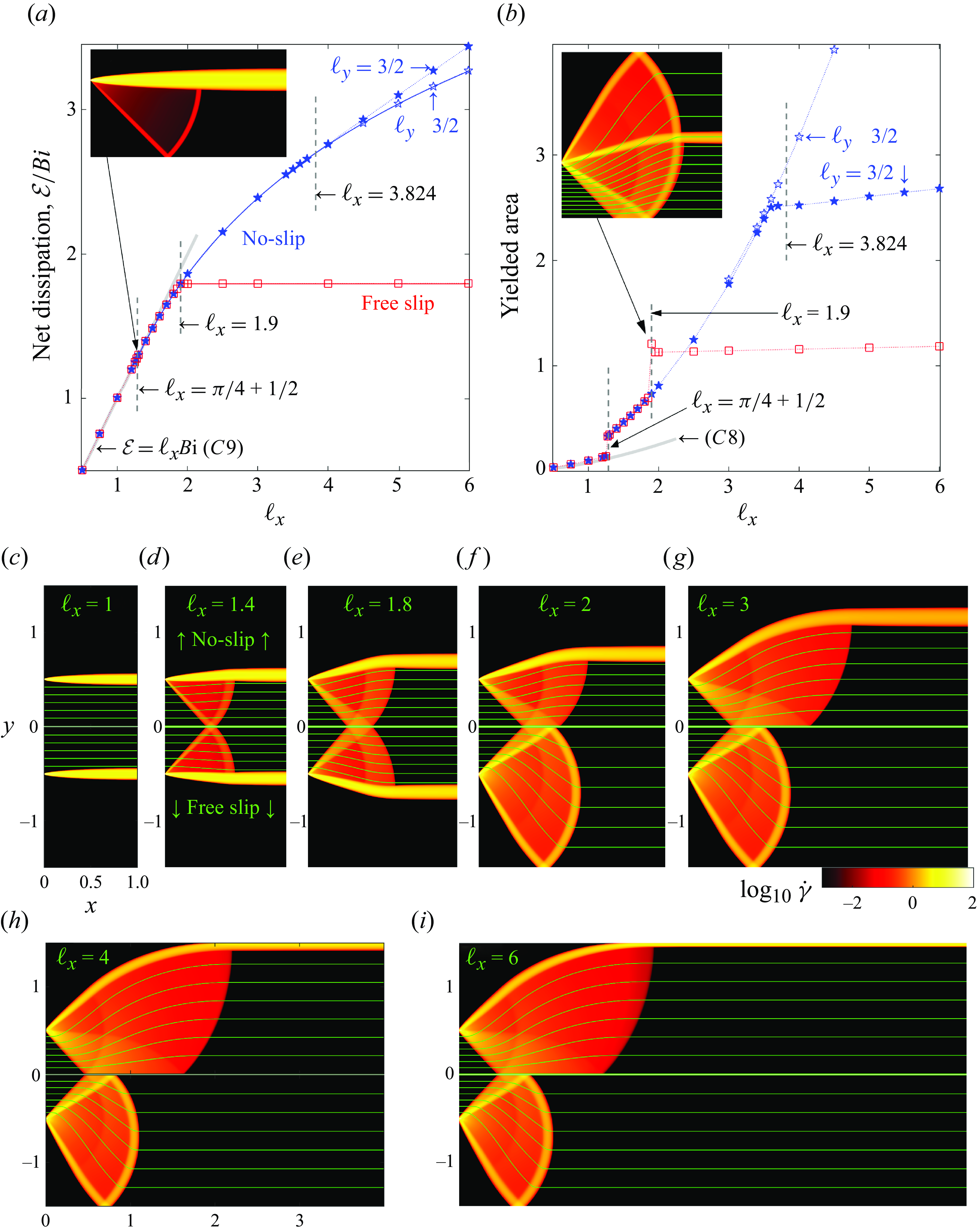
Figure 4. Viscoplastic jets for $(\textit{Bi},\ell _y)=(2048, {3}/{2})$
and varying
$(\textit{Bi},\ell _y)=(2048, {3}/{2})$
and varying $\ell _x$
. (a) Net dissipation rate and (b) area of the yielded regions for
$\ell _x$
. (a) Net dissipation rate and (b) area of the yielded regions for $y\gt 0$
, plotted against
$y\gt 0$
, plotted against $\ell _x$
. (c)–(i) Density maps of
$\ell _x$
. (c)–(i) Density maps of $\log _{10}{\dot \gamma }$
on the
$\log _{10}{\dot \gamma }$
on the $(x,y)$
-plane for the values of
$(x,y)$
-plane for the values of $\ell _x$
indicated. For each
$\ell _x$
indicated. For each $\ell _x$
, two solutions are shown: for the upper (filled blue stars in (a,b)), no-slip conditions are applied at
$\ell _x$
, two solutions are shown: for the upper (filled blue stars in (a,b)), no-slip conditions are applied at $y=\pm \ell _y$
; for the lower (open red squares in (a,b)), free-slip conditions are used instead. The insets in (a,b) show transitional, free-slip solutions at
$y=\pm \ell _y$
; for the lower (open red squares in (a,b)), free-slip conditions are used instead. The insets in (a,b) show transitional, free-slip solutions at $\ell _x=1.275$
and
$\ell _x=1.275$
and $\ell _x=1.9$
. Open (blue) stars in (a)–(b) represent solutions with
$\ell _x=1.9$
. Open (blue) stars in (a)–(b) represent solutions with $\ell _y\gg 3/2$
, for which the yielded regions do not touch the top and bottom boundaries. The grey lines in (a,b) show the predictions in (C8)–(C9). The solid blue and red lines in (a) show predictions for
$\ell _y\gg 3/2$
, for which the yielded regions do not touch the top and bottom boundaries. The grey lines in (a,b) show the predictions in (C8)–(C9). The solid blue and red lines in (a) show predictions for $\mathcal{E}$
based on the slipline fields in figure 6(a). The vertical dashed lines at
$\mathcal{E}$
based on the slipline fields in figure 6(a). The vertical dashed lines at $\ell _x=({\pi }/{4})+(1/2)$
and
$\ell _x=({\pi }/{4})+(1/2)$
and $\ell _x\approx 1.9$
indicate the flow pattern transitions arising when one of the plugs breaks; that at
$\ell _x\approx 1.9$
indicate the flow pattern transitions arising when one of the plugs breaks; that at $\ell _x=3.824$
indicates where the slipline solution predicts that the yielded region collides with the walls at
$\ell _x=3.824$
indicates where the slipline solution predicts that the yielded region collides with the walls at $y=\pm \ell _y$
.
$y=\pm \ell _y$
.
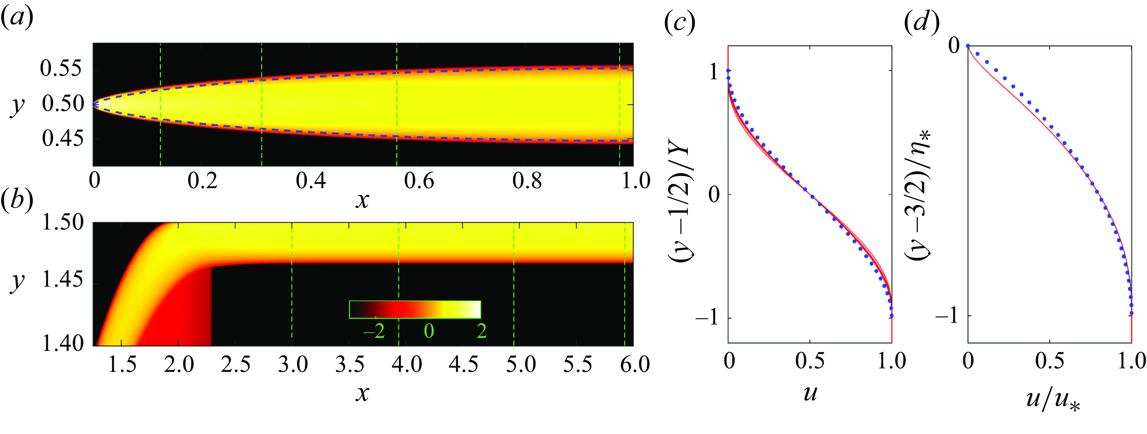
Figure 5. (a,c) The viscoplastic shear layer for $\ell _x=1$
(cf. figure 4
c), and (b,d) the wall boundary layer for
$\ell _x=1$
(cf. figure 4
c), and (b,d) the wall boundary layer for $\ell _x=6$
(cf. figure 4
i). The vertical dashed lines in (a,b) show the cuts at which the horizontal velocity profiles of (b,d) are drawn. The dashed curves in (a) shows the yield surfaces predicted by shear-layer theory (§ C.1.1). In (c), the velocity profiles (shown by red lines) are collapsed by shifting each by
$\ell _x=6$
(cf. figure 4
i). The vertical dashed lines in (a,b) show the cuts at which the horizontal velocity profiles of (b,d) are drawn. The dashed curves in (a) shows the yield surfaces predicted by shear-layer theory (§ C.1.1). In (c), the velocity profiles (shown by red lines) are collapsed by shifting each by $(1/2)$
, then plotting them against
$(1/2)$
, then plotting them against $\zeta =(y-(1/2))/Y$
, where
$\zeta =(y-(1/2))/Y$
, where $Y$
is the local half-width of the shear layer. In (d), the profiles are collapsed by scaling
$Y$
is the local half-width of the shear layer. In (d), the profiles are collapsed by scaling $u$
by the plug speed
$u$
by the plug speed $u_*$
, and then plotting the curves against
$u_*$
, and then plotting the curves against $\zeta =(y- (3/2)/\eta _*$
, where
$\zeta =(y- (3/2)/\eta _*$
, where $\eta _*$
is the local boundary-layer thickness. The blue dots in (c,d) show the predictions
$\eta _*$
is the local boundary-layer thickness. The blue dots in (c,d) show the predictions $(1/2)-(1/4)\zeta (3-\zeta ^2)$
(§§ C.1.1) and
$(1/2)-(1/4)\zeta (3-\zeta ^2)$
(§§ C.1.1) and $(2+\zeta )\zeta$
(C.1.2).
$(2+\zeta )\zeta$
(C.1.2).
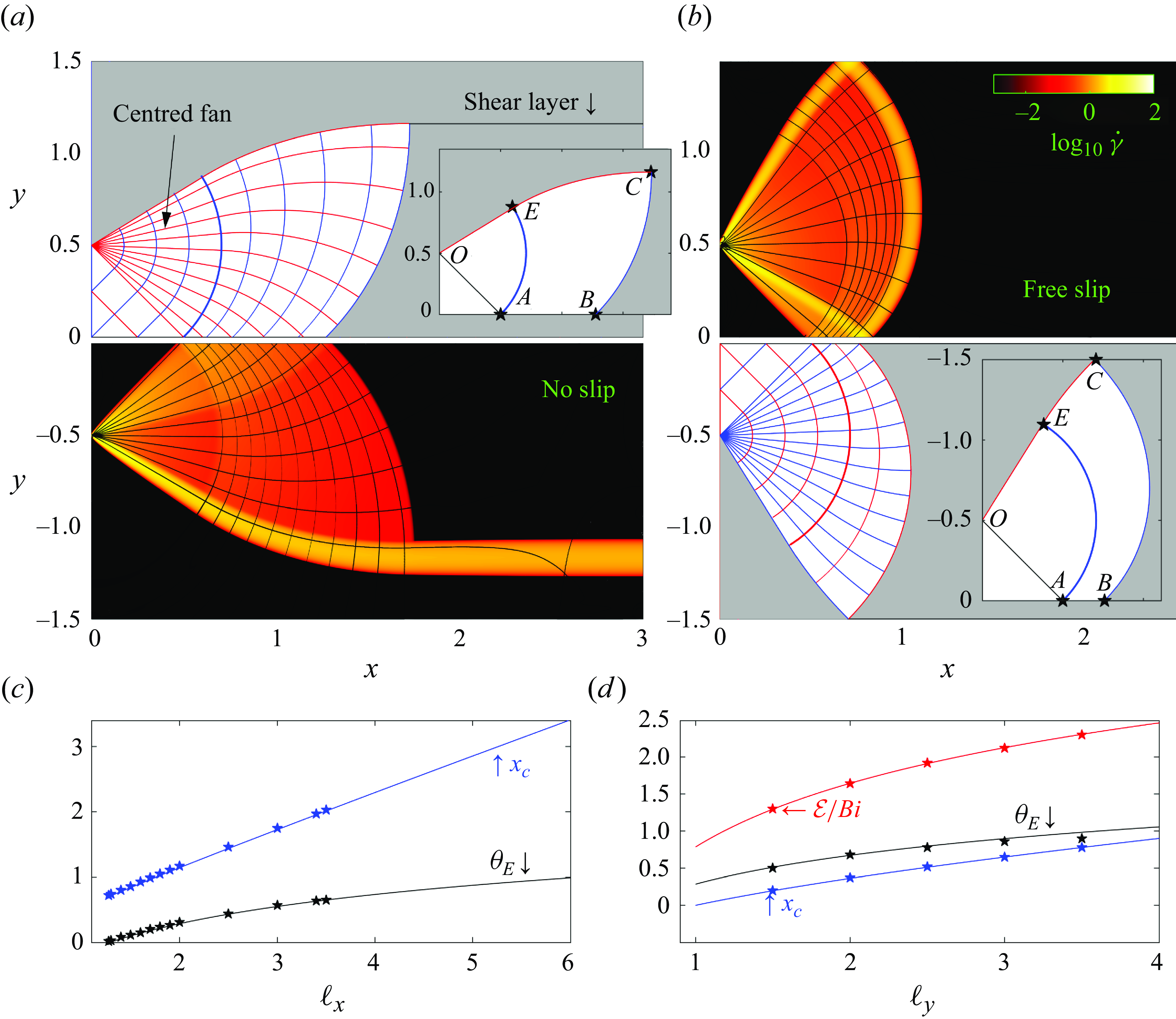
Figure 6. The two slipline fields for $\ell _x=3$
(cf. figure 4
g) for the (b) no-slip and (c) free-slip cases. Additional diagnostics are plotted in (c,d). In (a,b), half of the domain shows the numerical solution for
$\ell _x=3$
(cf. figure 4
g) for the (b) no-slip and (c) free-slip cases. Additional diagnostics are plotted in (c,d). In (a,b), half of the domain shows the numerical solution for $\log _{10}{\dot \gamma }$
along with reconstructions of the curves of constant
$\log _{10}{\dot \gamma }$
along with reconstructions of the curves of constant $p\pm 2\textit{Bi}\theta$
, and the insets display the geometry of the yielded regions and some special points of the slipline construction. For (c), we plot the
$p\pm 2\textit{Bi}\theta$
, and the insets display the geometry of the yielded regions and some special points of the slipline construction. For (c), we plot the $x-$
position of point
$x-$
position of point $C$
(
$C$
( $x_{_C}$
) and the slipline angle
$x_{_C}$
) and the slipline angle $(\theta _{_E}$
) at point
$(\theta _{_E}$
) at point $E$
against
$E$
against $\ell _x$
for no-slip solutions with
$\ell _x$
for no-slip solutions with $\ell _y=3$
. In (d), the scaled dissipation rate
$\ell _y=3$
. In (d), the scaled dissipation rate $\mathcal{E}/\textit{Bi}$
,
$\mathcal{E}/\textit{Bi}$
, $\theta _{_E}$
and
$\theta _{_E}$
and $x_{_C}$
are plotted against
$x_{_C}$
are plotted against $\ell _y$
, for free-slip solutions with
$\ell _y$
, for free-slip solutions with $\ell _y=1.5$
. The stars in (c,d) display corresponding results from the numerical solutions (with
$\ell _y=1.5$
. The stars in (c,d) display corresponding results from the numerical solutions (with $x_{_C}$
measured from the right-hand border of the plastic region in (a), then from the centre of the shear layer at
$x_{_C}$
measured from the right-hand border of the plastic region in (a), then from the centre of the shear layer at $y=\ell _y$
in (b) and
$y=\ell _y$
in (b) and $\theta _{_E}$
from the centre of the upper shear layer at
$\theta _{_E}$
from the centre of the upper shear layer at $x=(1/4)$
).
$x=(1/4)$
).
As the domain becomes longer, the stresses exerted on the moving plug increase; eventually, this increase causes the plug to break. A region of almost perfectly plastic deformation then appears near the inlet that allows the jet to adjust its width (figure 4 d,e). This widening reduces the net dissipation rate below that expected for an unbroken plug (figure 4 a), and abruptly increases the area of yielded plug (figure 4 b). Evidently, the widening of the jet is sufficient to reduce the velocity jumps across the shear layers, and the net dissipation rate within them, despite the lengthening of those layers and the additional dissipation incurred over the plastic region.
As illustrated in figure 6(a,b), the perfectly plastic flow can be described by slipline theory: much as for Prandtl’s punch, two centred fans emerge from the edges of the inlet, with a triangular wedge between them. Indeed, the intrusion can be viewed as an indentation problem, with different boundary conditions applying on the left wall. The fans extend outwards and meet along the centreline of the jet; the slipline pattern then continues out to the right, with all the sliplines becoming curved due to the symmetry condition along $y=0$
(
$y=0$
( $|\theta |=({1}/{4})\pi$
). The plastic region terminates to the right along a final slipline that fronts the widened moving plug. Shear layers continue to buffer the jet from above and below. More details of the construction of the slipline field are given in Appendix B. Note that the checkerboard of sliplines filling the wedge at the inlet, in combination with the rigid-body inflow velocity, allows that region to solidify into another example of an serendipitous plug. A different example, in which the inflow is not rigid and the checkerboard remains fully plastic, is presented below in § 4.5.
$|\theta |=({1}/{4})\pi$
). The plastic region terminates to the right along a final slipline that fronts the widened moving plug. Shear layers continue to buffer the jet from above and below. More details of the construction of the slipline field are given in Appendix B. Note that the checkerboard of sliplines filling the wedge at the inlet, in combination with the rigid-body inflow velocity, allows that region to solidify into another example of an serendipitous plug. A different example, in which the inflow is not rigid and the checkerboard remains fully plastic, is presented below in § 4.5.
Figure 6(b,c) also illustrates the slipline field reconstructed directly from the numerical solutions, by plotting the curves of constant $p\pm \textit{Bi} \tan ^{-1}({\tau _{_{\textit{XX}}}}/{\tau _{_{\textit{XY}}}})$
(cf. equations (3.15)). This more practical strategy to determine the sliplines successfully confirms most of the details of the slipline field, but breaks down in the shear layers and plugs, and fails to trace all the sliplines in the fans. An example is which the reconstruction is even poorer will be encountered later in figure 10(b).
$p\pm \textit{Bi} \tan ^{-1}({\tau _{_{\textit{XX}}}}/{\tau _{_{\textit{XY}}}})$
(cf. equations (3.15)). This more practical strategy to determine the sliplines successfully confirms most of the details of the slipline field, but breaks down in the shear layers and plugs, and fails to trace all the sliplines in the fans. An example is which the reconstruction is even poorer will be encountered later in figure 10(b).
From the slipline solution, one can construct the force balance on the widened plug, which controls the size of the plastic region. Appendix B.2 summarises the details of this calculation, which provides predictions for a number of key characteristics of the flow pattern, as plotted in figures 4(a) and 6(b,c). For example, the net dissipation rate can be determined, either by a direct calculation using Geiringer’s equations (3.16), or by exploiting the power balance in (3.12) and calculating the power input along the borders of the slipline pattern.
The analysis of the slipline patterns also predicts the domain length at which the uninterrupted moving plug breaks: the critical value is $\ell _x\sim (1/4)\pi +(1/2)$
, as seen in figure 4(a,b). Because sudden jumps arise in the properties of the flow pattern at this transition (including the area of the yielded region), owing to the breakage of the plug, we refer to this type of bifurcation as ‘first order’, following the terminology of phase-transition theory. As we shall see below, continuous, or ‘second-order’ bifurcations are also possible, that do not involve the breakage of any plug. Note that the transition for the numerical solutions in figure 4 is slightly shifted and ‘blurred’: the finite Bingham number used for the computations adjusts the domain length at which the plug breaks and appears to lead to flow patterns with mixed character over a narrow window surrounding that transition (see the inset in figure 4
a). However, it is hard to tell whether this latter feature is genuine or an artefact of the numerical scheme, the solution having perhaps failed to properly converge (see Appendix A).
$\ell _x\sim (1/4)\pi +(1/2)$
, as seen in figure 4(a,b). Because sudden jumps arise in the properties of the flow pattern at this transition (including the area of the yielded region), owing to the breakage of the plug, we refer to this type of bifurcation as ‘first order’, following the terminology of phase-transition theory. As we shall see below, continuous, or ‘second-order’ bifurcations are also possible, that do not involve the breakage of any plug. Note that the transition for the numerical solutions in figure 4 is slightly shifted and ‘blurred’: the finite Bingham number used for the computations adjusts the domain length at which the plug breaks and appears to lead to flow patterns with mixed character over a narrow window surrounding that transition (see the inset in figure 4
a). However, it is hard to tell whether this latter feature is genuine or an artefact of the numerical scheme, the solution having perhaps failed to properly converge (see Appendix A).
In fact, there are actually two suites of computations shown in figure 4: one with no-slip walls at $y=\pm \ell _y$
, the other with free slip there. As long as
$y=\pm \ell _y$
, the other with free slip there. As long as $\ell _x$
remains less than about
$\ell _x$
remains less than about $1.9$
, the two sets of solutions are identical. In other words, two different problems have the same solution. This coincidence arises because of the cloaking effect of the plug that intervenes between the flowing region and the wall for
$1.9$
, the two sets of solutions are identical. In other words, two different problems have the same solution. This coincidence arises because of the cloaking effect of the plug that intervenes between the flowing region and the wall for $\ell _x \lesssim 1.9$
: if the wall lies inside a plug, that entire region is rigid and so the conditions applying upon the wall, and even its shape are irrelevant. This notion of cloaking dates back at least to Oldroyd (see Balmforth, Craster & Hewitt (Reference Balmforth, Craster and Hewitt2021)), and has been considered in detail for the motion of differently shaped particles encased in viscoplastic fluid (Chaparian & Frigaard Reference Chaparian and Frigaard2017a
,Reference Chaparian and Frigaard
b
). The difference between the two cases that emerges for longer domains arises because the plug breaks for free-slip walls at
$\ell _x \lesssim 1.9$
: if the wall lies inside a plug, that entire region is rigid and so the conditions applying upon the wall, and even its shape are irrelevant. This notion of cloaking dates back at least to Oldroyd (see Balmforth, Craster & Hewitt (Reference Balmforth, Craster and Hewitt2021)), and has been considered in detail for the motion of differently shaped particles encased in viscoplastic fluid (Chaparian & Frigaard Reference Chaparian and Frigaard2017a
,Reference Chaparian and Frigaard
b
). The difference between the two cases that emerges for longer domains arises because the plug breaks for free-slip walls at $\ell _x\approx 1.9$
, decloaking the wall (see below in § 4.3).
$\ell _x\approx 1.9$
, decloaking the wall (see below in § 4.3).
4.2. Wide domains; no-slip walls
For longer domain lengths, the solutions depend on the boundary condition applied along the top and bottom boundaries (see e.g. figure 4
a,b,f). With a no-slip condition, the jet continues to widen gradually until it meets the walls at $y=\pm \ell _y$
, for domains lengths near
$y=\pm \ell _y$
, for domains lengths near $\ell _x\approx 3.6$
. Thereafter, as in figure 4(h), the bordering shear layers narrow to become described by the viscoplastic wall-boundary-layer theory of § C.1.2. That wall layer is predicted to have constant thickness and a parabolic velocity profile. The former feature is well reproduced by the numerical solution, as illustrated in figure 5(b). The parabolic velocity profile is less well reproduced, however; see figure 5(d). The discrepancy here arises not because the boundary-layer flow takes a different form to that predicted, but because of the algorithm used to compute the solutions: the algorithm exploits a Fourier cosine series in
$\ell _x\approx 3.6$
. Thereafter, as in figure 4(h), the bordering shear layers narrow to become described by the viscoplastic wall-boundary-layer theory of § C.1.2. That wall layer is predicted to have constant thickness and a parabolic velocity profile. The former feature is well reproduced by the numerical solution, as illustrated in figure 5(b). The parabolic velocity profile is less well reproduced, however; see figure 5(d). The discrepancy here arises not because the boundary-layer flow takes a different form to that predicted, but because of the algorithm used to compute the solutions: the algorithm exploits a Fourier cosine series in $y$
, and the solutions only satisfy a no-slip condition at
$y$
, and the solutions only satisfy a no-slip condition at $y=\ell _y$
after the addition of a numerical ‘sponge layer’ at the top boundary (spanning
$y=\ell _y$
after the addition of a numerical ‘sponge layer’ at the top boundary (spanning $\ell _y\lt y\lt 1.1\ell _y$
). Over the sponge, the yield stress and viscosity are artificially increased to suppress motion. In finer detail, however, this device does not fully incorporate no slip, leaving a velocity profile with noticeable departures from parabolic form. In other words, the boundary-layer theory exposes an artefact in the numerical solution.
$\ell _y\lt y\lt 1.1\ell _y$
). Over the sponge, the yield stress and viscosity are artificially increased to suppress motion. In finer detail, however, this device does not fully incorporate no slip, leaving a velocity profile with noticeable departures from parabolic form. In other words, the boundary-layer theory exposes an artefact in the numerical solution.
When the yielded region reaches the no-slip wall near $\ell _x\approx 3.6$
, the containment of the flow by the no-slip boundaries limits the yielded area and enhances the dissipation rate above what would have been incurred had there been no collision with the wall. Both feature are illustrated in figure 4(a,b), in which
$\ell _x\approx 3.6$
, the containment of the flow by the no-slip boundaries limits the yielded area and enhances the dissipation rate above what would have been incurred had there been no collision with the wall. Both feature are illustrated in figure 4(a,b), in which $\mathcal{E}$
and the yielded area are compared with corresponding data for solutions with larger
$\mathcal{E}$
and the yielded area are compared with corresponding data for solutions with larger $\ell _y$
. The collision of the yielded region with the wall indicates a second transition in flow pattern for the no-slip problem. In this case, however, no plug breaks and the pattern properties change continuously. The transition is therefore second-order.
$\ell _y$
. The collision of the yielded region with the wall indicates a second transition in flow pattern for the no-slip problem. In this case, however, no plug breaks and the pattern properties change continuously. The transition is therefore second-order.
According to the slipline solution, the widened jet meets the walls when $\ell _x\approx 3.824$
for this specific value of
$\ell _x\approx 3.824$
for this specific value of $\ell _y$
. Because the shear layers have finite thickness in the numerical solutions, the transition occurs at the slightly smaller value of
$\ell _y$
. Because the shear layers have finite thickness in the numerical solutions, the transition occurs at the slightly smaller value of $\ell _x\approx 3.6$
. Once the yielded region collides with the wall, its structure becomes fixed (see figure 4
h,i), with the lengthening of the domain in
$\ell _x\approx 3.6$
. Once the yielded region collides with the wall, its structure becomes fixed (see figure 4
h,i), with the lengthening of the domain in $x$
serving only to impact the length and thickness of the wall layer.
$x$
serving only to impact the length and thickness of the wall layer.
4.3. Wide domains; free-slip walls
For free-slip walls, the solutions develop differently with increasing domain length: at $\ell _x\approx 1.9$
, the yielded region widens abruptly, with the moving plug then filling the entire cross-stream domain (e.g. figure 4
f). The sudden jump in yielded area indicates that the transition is again first-order. In this case, the transition arises because the stationary plug that cloaks the wall for smaller
$\ell _x\approx 1.9$
, the yielded region widens abruptly, with the moving plug then filling the entire cross-stream domain (e.g. figure 4
f). The sudden jump in yielded area indicates that the transition is again first-order. In this case, the transition arises because the stationary plug that cloaks the wall for smaller $\ell _x$
breaks suddenly. This de-cloaking event leaves a pattern for
$\ell _x$
breaks suddenly. This de-cloaking event leaves a pattern for $\ell _x\gt 1.9$
containing sliplines that meet the wall at
$\ell _x\gt 1.9$
containing sliplines that meet the wall at $45^\circ$
(see figure 4
f); the new slipline pattern is shown in more detail in figure 6(b). The inset of figure 4(b) further illustrates how the transition again becomes blurred for the finite-
$45^\circ$
(see figure 4
f); the new slipline pattern is shown in more detail in figure 6(b). The inset of figure 4(b) further illustrates how the transition again becomes blurred for the finite- $\textit{Bi}$
computation, with patterns of mixed character appearing once more.
$\textit{Bi}$
computation, with patterns of mixed character appearing once more.
In regard to the minimisation of $\mathcal{E}$
, the widening of the moving plug incurs no additional dissipation at the top and bottom boundaries in view of the free-slip condition that holds there; the plug now freely slides. This means that, once the domain becomes sufficiently wide, the dissipation rate can be kept lower by eliminating the shear layers of the moving plug, despite the broadening of the perfectly plastic flow region, paving the way for the flow transition at
$\mathcal{E}$
, the widening of the moving plug incurs no additional dissipation at the top and bottom boundaries in view of the free-slip condition that holds there; the plug now freely slides. This means that, once the domain becomes sufficiently wide, the dissipation rate can be kept lower by eliminating the shear layers of the moving plug, despite the broadening of the perfectly plastic flow region, paving the way for the flow transition at $\ell _x\approx 1.9$
. The switch is reflected by a kink in the plot of
$\ell _x\approx 1.9$
. The switch is reflected by a kink in the plot of $\mathcal{E}$
near
$\mathcal{E}$
near $\ell _x\approx 1.9$
(figure 4
a), and a corresponding jump in the yielded area (figure 4(b)). Both metrics become independent of
$\ell _x\approx 1.9$
(figure 4
a), and a corresponding jump in the yielded area (figure 4(b)). Both metrics become independent of $\ell _x$
beyond the transition because the sliding plug shields the extended yielded zone from whatever lies to the right, and can accommodate any increase in domain length (see figure 4
f–
4(i)).
$\ell _x$
beyond the transition because the sliding plug shields the extended yielded zone from whatever lies to the right, and can accommodate any increase in domain length (see figure 4
f–
4(i)).
Note that the density plots of the strain rate in figure 4 display substructure beyond the identification of the yielded regions for both no-slip and free-slip top walls: the shear and boundary layers bordering the plastically deforming region are highlighted by elevated levels of $\dot \gamma$
. In addition, enhanced dissipation arises at the junctions between different sections of the slipline pattern due to the smoothing of the associated discontinuities in the plastic velocity field. Altogether, the viscoplastic shear and boundary layers in combination with the structure of the slipline field rationalise the form of the flow pattern.
$\dot \gamma$
. In addition, enhanced dissipation arises at the junctions between different sections of the slipline pattern due to the smoothing of the associated discontinuities in the plastic velocity field. Altogether, the viscoplastic shear and boundary layers in combination with the structure of the slipline field rationalise the form of the flow pattern.
4.4. Further details of the plugs; stress indeterminacy
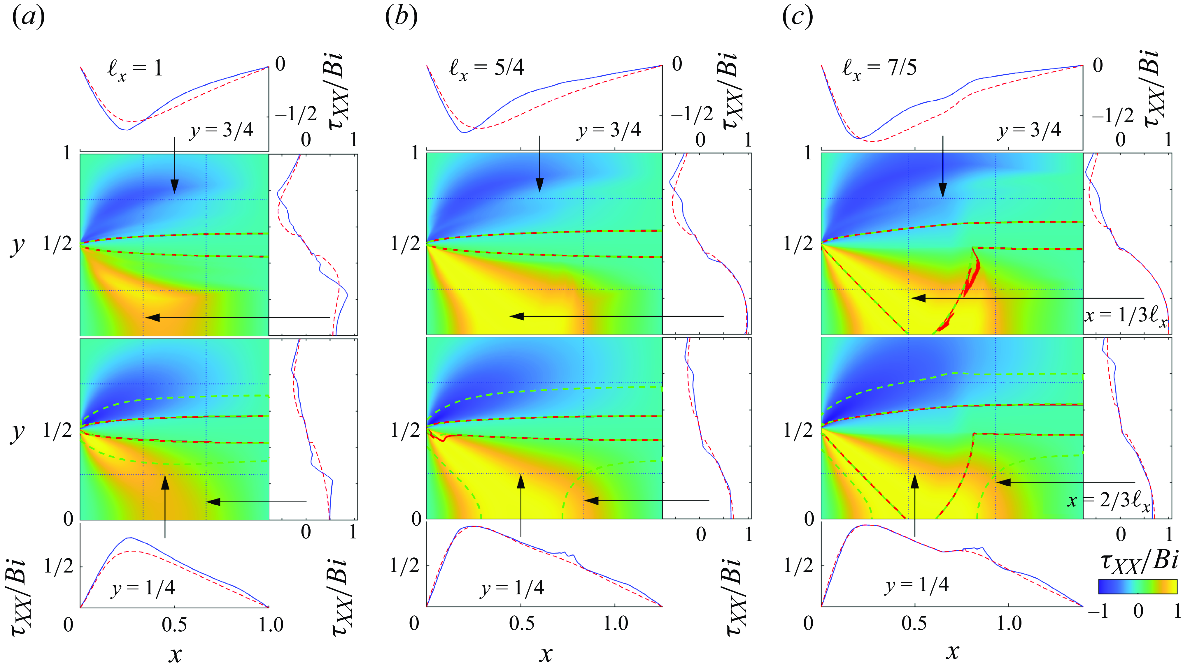
Figure 7. The scaled stress component ${\tau _{_{\textit{XX}}}}/\textit{Bi}$
for (a)
${\tau _{_{\textit{XX}}}}/\textit{Bi}$
for (a) $\ell _x=1$
, (b)
$\ell _x=1$
, (b) $5/4$
and (c)
$5/4$
and (c) $ 7/5$
, showing
$ 7/5$
, showing $y\gt 0$
. The upper density plot is computed with the augmented Lagrangian scheme; the lower one exploits a regularisation of the constitutive law (Papanastasiou (A1), with
$y\gt 0$
. The upper density plot is computed with the augmented Lagrangian scheme; the lower one exploits a regularisation of the constitutive law (Papanastasiou (A1), with $\beta =10^{4}$
). The red contours indicate where
$\beta =10^{4}$
). The red contours indicate where $\tau =\textit{Bi}$
; the dashed green contours identify curves of constant
$\tau =\textit{Bi}$
; the dashed green contours identify curves of constant ${\dot \gamma }=10^{-3}$
and
${\dot \gamma }=10^{-3}$
and $10^{-4}$
. Cuts of
$10^{-4}$
. Cuts of ${\tau _{_{\textit{XX}}}}/\textit{Bi}$
along
${\tau _{_{\textit{XX}}}}/\textit{Bi}$
along $x=(1/3)\ell _x$
and
$x=(1/3)\ell _x$
and $(2/3)\ell _x$
are plotted to the right of the density maps (upper and lower panels, respectively); cuts along
$(2/3)\ell _x$
are plotted to the right of the density maps (upper and lower panels, respectively); cuts along $y=(1/4)$
and
$y=(1/4)$
and $3/4$
are plotted below and above (respectively). In these cuts, the results with the augmented Lagrangian algorithm are plotted as solid blue, and for regularisation with dashed red.
$3/4$
are plotted below and above (respectively). In these cuts, the results with the augmented Lagrangian algorithm are plotted as solid blue, and for regularisation with dashed red.
Over the plugs in figure 4, the indeterminacy of the stress state implies that multiple solutions should be possible, even though the precise numerical algorithm employed selects a particular one. This feature is illustrated in figure 7 where computations with the augmented Lagrangian algorithm for $\ell _x=1$
,
$\ell _x=1$
, $5/4$
and
$5/4$
and $ 7/5$
are compared with corresponding solutions computed using the popular Papanastasiou regularisation (see Appendix A). The two agree over the yielded regions, provided the regularisation parameter
$ 7/5$
are compared with corresponding solutions computed using the popular Papanastasiou regularisation (see Appendix A). The two agree over the yielded regions, provided the regularisation parameter $\beta$
is chosen to be sufficiently large. In panels (a,b), the yielded region consists of only the shear layer; for the example in panel (c), the yielded region is larger, the central plug having broken.
$\beta$
is chosen to be sufficiently large. In panels (a,b), the yielded region consists of only the shear layer; for the example in panel (c), the yielded region is larger, the central plug having broken.
Over the plugs the two stress solutions do not agree, because the augmented Lagrangian scheme converges to a stress–velocity solution that does not satisfy the constitutive law of the generalised Newtonian fluid employed by the regularised scheme. However, near the bifurcation at $\ell _x\sim (1/4)\pi +(1/2)$
(panel (b)), the range of possible stress states evidently becomes more restricted. As a consequence, the two stress solutions align more closely over the impending yielded region. At bifurcation, the range of possible stress solutions narrows to the single, unique, yielded solution, which correspond to the mode of failure of the moving plug.
$\ell _x\sim (1/4)\pi +(1/2)$
(panel (b)), the range of possible stress states evidently becomes more restricted. As a consequence, the two stress solutions align more closely over the impending yielded region. At bifurcation, the range of possible stress solutions narrows to the single, unique, yielded solution, which correspond to the mode of failure of the moving plug.
Figure 7 also highlights two other practical issues with the computations: for the augmented Lagrangian scheme, the yield surface predicted by $\tau =\textit{Bi}$
can be somewhat rough; it is arguably better to use a contour of a small value of
$\tau =\textit{Bi}$
can be somewhat rough; it is arguably better to use a contour of a small value of $\log _{10}{\dot \gamma }$
. Indeed, we have followed this practice everywhere but in figure 7. On the other hand, with a regularisation of the viscosity, strain rates of order
$\log _{10}{\dot \gamma }$
. Indeed, we have followed this practice everywhere but in figure 7. On the other hand, with a regularisation of the viscosity, strain rates of order $\beta ^{-1}$
are not relevant to a yield-stress fluid and it can be awkward to detect true yield surfaces. For this algorithm, figure 7 demonstrates that it is better to use either
$\beta ^{-1}$
are not relevant to a yield-stress fluid and it can be awkward to detect true yield surfaces. For this algorithm, figure 7 demonstrates that it is better to use either $\tau =\textit{Bi}$
or a contour of constant
$\tau =\textit{Bi}$
or a contour of constant $1\gg {\dot \gamma }\gg \beta ^{-1}$
to locate effective yield surfaces. Even with such choices, however, the scheme fails to capture all of the yield surface in figure 7(b). Other practical issues with regularising the constitutive model are discussed by Frigaard & Nouar (Reference Frigaard and Nouar2005).
$1\gg {\dot \gamma }\gg \beta ^{-1}$
to locate effective yield surfaces. Even with such choices, however, the scheme fails to capture all of the yield surface in figure 7(b). Other practical issues with regularising the constitutive model are discussed by Frigaard & Nouar (Reference Frigaard and Nouar2005).
4.5. Indentation; the appearance of stress discontinuities
Prandtl’s punch problem in figure 2(b) corresponds to a minor variation on the jet configuration, in which we apply different boundary conditions on the left boundary and take the domain to be sufficiently large that fluid plugs up well before reaching all the other boundaries. In fact, a simple periodic version of Prandtl’s punch follows from adopting free-slip conditions at $y=\pm \ell _y$
and setting
$y=\pm \ell _y$
and setting $u(0,y)=u_0(y)$
, where
$u(0,y)=u_0(y)$
, where $u_0(y)$
is a
$u_0(y)$
is a $2\ell _y-$
periodic function with zero average. Figure 8 presents solutions for such a problem, in which
$2\ell _y-$
periodic function with zero average. Figure 8 presents solutions for such a problem, in which $u_0(y)$
is prescribed as either a square wave or a sine function. For large
$u_0(y)$
is prescribed as either a square wave or a sine function. For large $\textit{Bi}$
, we arrive at solutions for which we recognise a periodic repetition of the fans of Prandtl’s slipline pattern (panels (a,b), left-hand density plots). Much further from the plastic limit, at lower
$\textit{Bi}$
, we arrive at solutions for which we recognise a periodic repetition of the fans of Prandtl’s slipline pattern (panels (a,b), left-hand density plots). Much further from the plastic limit, at lower $\textit{Bi}$
, some of the features remain (panels (a,b), right-hand density plots).
$\textit{Bi}$
, some of the features remain (panels (a,b), right-hand density plots).
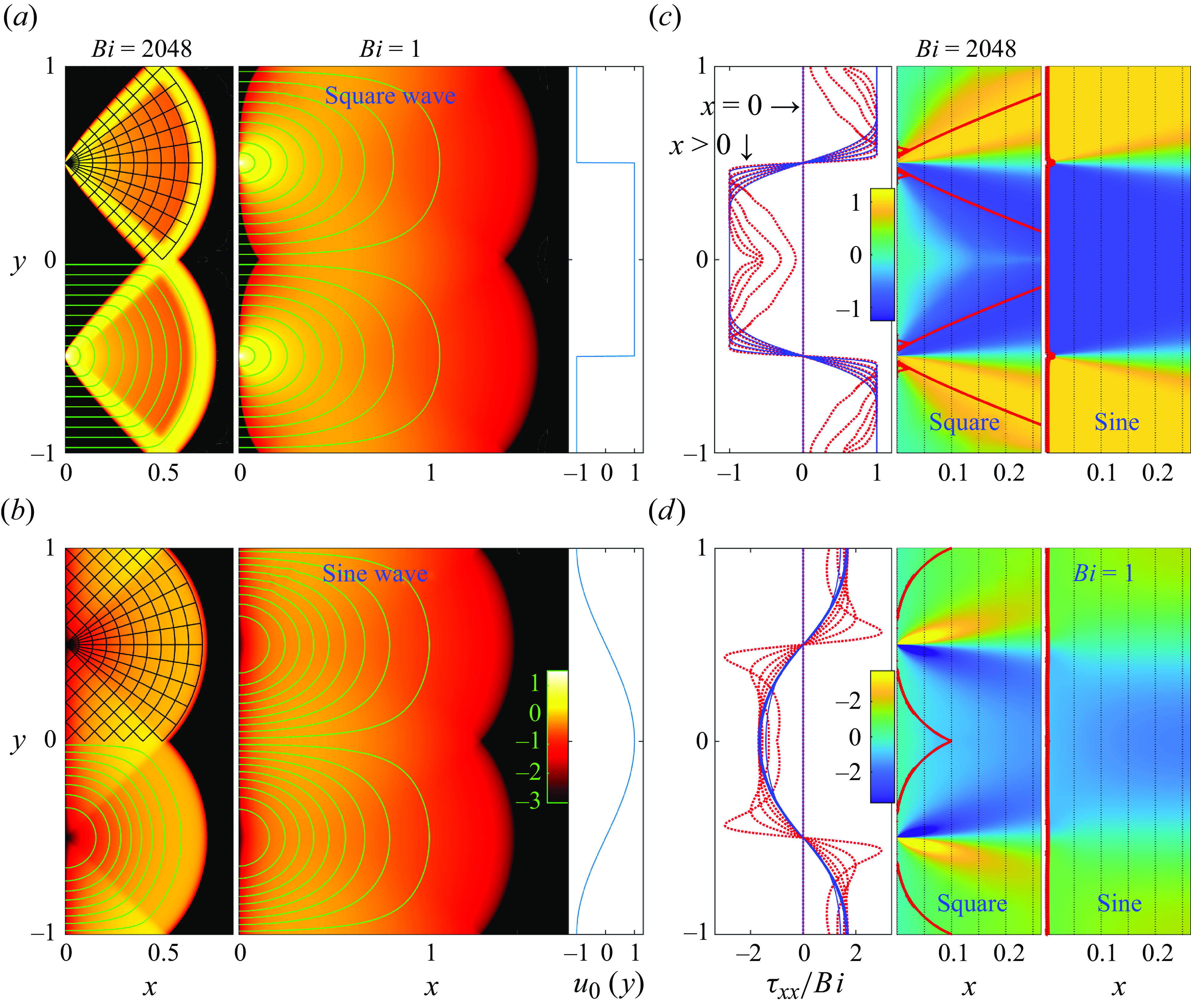
Figure 8. Indentation solutions for $u(0,y)=u_0(y)$
with (a)
$u(0,y)=u_0(y)$
with (a) $u_0=$
sgn
$u_0=$
sgn $((1/2)-|y|)$
and (b)
$((1/2)-|y|)$
and (b) $u_0=\sin y$
(and symmetry conditions along
$u_0=\sin y$
(and symmetry conditions along $y=\pm 1$
and
$y=\pm 1$
and $x=\ell _x$
). For each case, solutions for
$x=\ell _x$
). For each case, solutions for $\textit{Bi}=1$
and
$\textit{Bi}=1$
and $2048$
are shown, plotting
$2048$
are shown, plotting $\log _{10}{\dot \gamma }$
over the
$\log _{10}{\dot \gamma }$
over the $(x,y)$
-plane (with the same colour map). The green lines show sample streamlines; sliplines are plotted in black. In (c), the scaled stress component
$(x,y)$
-plane (with the same colour map). The green lines show sample streamlines; sliplines are plotted in black. In (c), the scaled stress component ${\tau _{_{\textit{XX}}}}/\textit{Bi}$
is shown for both solutions with
${\tau _{_{\textit{XX}}}}/\textit{Bi}$
is shown for both solutions with $\textit{Bi}=2048$
; the thicker (red) contour shows the yield surfaces. Cuts of
$\textit{Bi}=2048$
; the thicker (red) contour shows the yield surfaces. Cuts of ${\tau _{_{\textit{XX}}}}/\textit{Bi}$
are plotted to the left, taken from the vertical dotted lines on the density maps; the blue lines are for the sinusoid, red for the square wave. (d) A similar plot for the solutions with
${\tau _{_{\textit{XX}}}}/\textit{Bi}$
are plotted to the left, taken from the vertical dotted lines on the density maps; the blue lines are for the sinusoid, red for the square wave. (d) A similar plot for the solutions with $\textit{Bi}=1$
.
$\textit{Bi}=1$
.
Note that the velocity field over the triangular checkerboards in Prandtl’s solution is uniform, and so these regions are consistent with plugs. This remains true for the periodic version shown in figure 8(a) which uses the square-wave ‘indentation’, $u_0(y)=$
sgn
$u_0(y)=$
sgn $((1/2)-|y|)$
. By contrast, when
$((1/2)-|y|)$
. By contrast, when $u_0(y)=\sin y$
(figure 8
b), the velocity field over those regions is sheared and the checkerboards then add to the yielded area. In other words, the checkerboards again provide settings for serendipitous plugs.
$u_0(y)=\sin y$
(figure 8
b), the velocity field over those regions is sheared and the checkerboards then add to the yielded area. In other words, the checkerboards again provide settings for serendipitous plugs.
Aside from this difference, two solutions in figure 8 evidently possess the same stress solution for $\textit{Bi}\gg 1$
(see figure 8
c). This demonstrates another novel feature of viscoplastic flow near the plastic field: there can be multiple solutions with the same stress solution but different velocity field. This form of non-uniqueness is different from the cloaking effect of a plug, as it arises for yielded flow. The multiplicity is also only a feature of the plastic limit: for lower Bingham number (at
$\textit{Bi}\gg 1$
(see figure 8
c). This demonstrates another novel feature of viscoplastic flow near the plastic field: there can be multiple solutions with the same stress solution but different velocity field. This form of non-uniqueness is different from the cloaking effect of a plug, as it arises for yielded flow. The multiplicity is also only a feature of the plastic limit: for lower Bingham number (at $\textit{Bi}=1$
in figure 8
d), viscous effects distinguish the two solutions.
$\textit{Bi}=1$
in figure 8
d), viscous effects distinguish the two solutions.
The indentation problem illustrates yet another feature of the plastic limit: Prandtl’s solution demands that $\theta =\pm \frac \pi 4$
, or
$\theta =\pm \frac \pi 4$
, or ${\tau _{_{\textit{XY}}}}=0$
and
${\tau _{_{\textit{XY}}}}=0$
and $|{\tau _{_{\textit{XX}}}}|=\textit{Bi}$
, along the left wall. In fact, as seen in figure 8(c),
$|{\tau _{_{\textit{XX}}}}|=\textit{Bi}$
, along the left wall. In fact, as seen in figure 8(c), $\tau _{_{\textit{XX}}}$
jumps from
$\tau _{_{\textit{XX}}}$
jumps from $-\textit{Bi}$
to
$-\textit{Bi}$
to $\textit{Bi}$
as one passes through the centre of the fans. For the square-wave example, this stress distribution and jump is not significant, as the entire left boundary, barring the centres of the fans, lies within the plugged-up checkerboards. For the sinusoid, however, the velocity field through the checkerboards is inconsistent with rigid-body motion, leaving them yielded. But the velocity boundary condition and continuity demand
$\textit{Bi}$
as one passes through the centre of the fans. For the square-wave example, this stress distribution and jump is not significant, as the entire left boundary, barring the centres of the fans, lies within the plugged-up checkerboards. For the sinusoid, however, the velocity field through the checkerboards is inconsistent with rigid-body motion, leaving them yielded. But the velocity boundary condition and continuity demand $v=\partial v/\partial y = \partial u/\partial x=0 \quad {\rm at} \quad x=0$
. If the left-hand boundary were yielded, the last of these conditions implies that
$v=\partial v/\partial y = \partial u/\partial x=0 \quad {\rm at} \quad x=0$
. If the left-hand boundary were yielded, the last of these conditions implies that ${\tau _{_{\textit{XX}}}}=0$
, in disagreement with Prandtl’s solution. Thus, the stress field must contain a discontinuity along
${\tau _{_{\textit{XX}}}}=0$
, in disagreement with Prandtl’s solution. Thus, the stress field must contain a discontinuity along $x=0$
to rescue the slipline solution. Indeed, the cuts shown to the left of figure 8(c) provide numerical evidence that
$x=0$
to rescue the slipline solution. Indeed, the cuts shown to the left of figure 8(c) provide numerical evidence that $\tau _{_{\textit{XX}}}$
suddenly jumps from
$\tau _{_{\textit{XX}}}$
suddenly jumps from $\pm \textit{Bi}$
in
$\pm \textit{Bi}$
in $x\gt 0$
to zero at
$x\gt 0$
to zero at $x=0$
. As mentioned in § 3.4, such features are acceptable for a perfectly plastic material.
$x=0$
. As mentioned in § 3.4, such features are acceptable for a perfectly plastic material.
What is more surprising, however, is that the numerical solutions in figure 8 are not computed for the perfectly plastic problem, but with finite $\textit{Bi}$
. One might therefore imagine that the stress discontinuities are not true features of these numerical solutions, but become smoothed in some way by the addition of the viscous stress to the constitutive law. In fact, this is not the case: the solutions for
$\textit{Bi}$
. One might therefore imagine that the stress discontinuities are not true features of these numerical solutions, but become smoothed in some way by the addition of the viscous stress to the constitutive law. In fact, this is not the case: the solutions for $\textit{Bi}=1$
as well as those for
$\textit{Bi}=1$
as well as those for $\textit{Bi}=2048$
appear to share genuine stress discontinuities along
$\textit{Bi}=2048$
appear to share genuine stress discontinuities along $x=0$
. In other words, the viscous stress does not smooth out these feature, in conflict with one’s expectations from Stokes flow (where the strain rates and stresses are continuous for non-singular solutions). A closer inspection at figure 8(c,d) reveals how this is apparently accomplished: a yield surface with
$x=0$
. In other words, the viscous stress does not smooth out these feature, in conflict with one’s expectations from Stokes flow (where the strain rates and stresses are continuous for non-singular solutions). A closer inspection at figure 8(c,d) reveals how this is apparently accomplished: a yield surface with ${\dot \gamma }=0$
appears along
${\dot \gamma }=0$
appears along $x=0$
. Because of this yield line, the stress need no longer converge to
$x=0$
. Because of this yield line, the stress need no longer converge to ${\tau _{_{\textit{XX}}}}=0$
at
${\tau _{_{\textit{XX}}}}=0$
at $x=0$
for any
$x=0$
for any $\textit{Bi}$
.
$\textit{Bi}$
.
Stress discontinuities can also emerge at finite $\textit{Bi}$
within the flow domain. For example, Hewitt & Balmforth (Reference Hewitt and Balmforth2017) considered the viscoplastic version of Taylor’s swimming sheet, which is closely related to the indentation problems in figure 8, except that the left-hand boundary is no longer straight. At both large and order-one Bingham numbers, Hewitt & Balmforth (Reference Hewitt and Balmforth2017) present solutions with stress discontinuities.
$\textit{Bi}$
within the flow domain. For example, Hewitt & Balmforth (Reference Hewitt and Balmforth2017) considered the viscoplastic version of Taylor’s swimming sheet, which is closely related to the indentation problems in figure 8, except that the left-hand boundary is no longer straight. At both large and order-one Bingham numbers, Hewitt & Balmforth (Reference Hewitt and Balmforth2017) present solutions with stress discontinuities.
5. Flow between concentric cylinders
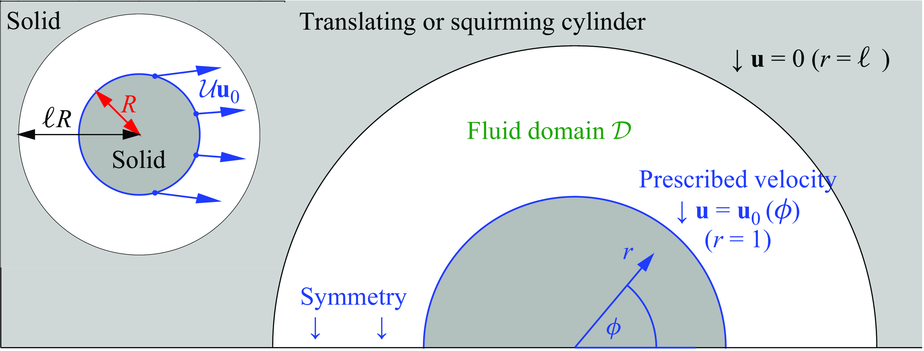
Figure 9. Sketch of the flow between concentric cylinders with prescribed surface velocities. The characteristic scales $\mathcal{L}$
and
$\mathcal{L}$
and $\mathcal{U}$
are set by the radius
$\mathcal{U}$
are set by the radius $R$
of the inner cylinder and a measure of its surface speed
$R$
of the inner cylinder and a measure of its surface speed $U$
. Again, symmetry about an axis is exploited to halve the computational domain.
$U$
. Again, symmetry about an axis is exploited to halve the computational domain.
Our second canonical problem, sketched in figure 9, describes the instantaneous flow between two cylinders induced by the motion of the inner surface. Because stresses decline away from the moving surface, one expects fluid to plug up well before the outer cylinder if the annular gap is sufficiently wide (cf. § 2). That wall is then cloaked, rendering its shape and precise position irrelevant. Consequently, in this limit the problem is equivalent to flow around a translating or rotating disk in an infinite viscoplastic medium (Randolph & Houlsby Reference Randolph and Houlsby1984; Tokpavi et al. Reference Tokpavi, Magnin and Jay2008; Hewitt & Balmforth Reference Hewitt and Balmforth2018). With a more complicated surface velocity, the problem also models a two-dimensional biological locomotor ‘squirming’ through viscoplastic fluid (Supekar et al. Reference Supekar, Hewitt and Balmforth2020). In the opposite limit, when the radii of the surfaces are much closer, the gap between them is narrow, and we arrive at a viscoplastic journal bearing (the eccentric version of which was considered by Hewitt & Balmforth (Reference Hewitt and Balmforth2012)).
For the examples we consider in this section, we adopt the radius of the inner cylinder as the length scale $\mathcal{L}$
(see figure 9), and prescribe its dimensional surface velocity by
$\mathcal{L}$
(see figure 9), and prescribe its dimensional surface velocity by
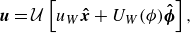 \begin{equation} \boldsymbol{u} = \mathcal{U} \left [ {u_{W}} \boldsymbol{\hat x} + {U_{W}}(\phi ) \boldsymbol{\hat \phi } \right ], \end{equation}
where $\phi$
denotes polar angle. That is,
$\phi$
denotes polar angle. That is, $\mathcal{U}{u_{W}}$
denotes the translation speed and
$\mathcal{U}{u_{W}}$
denotes the translation speed and $\mathcal{U}{U_{W}}(\phi )$
defines a specified angular velocity. The radius of the outer cylinder
$\mathcal{U}{U_{W}}(\phi )$
defines a specified angular velocity. The radius of the outer cylinder $\ell$
now becomes a parameter of the problem (along with
$\ell$
now becomes a parameter of the problem (along with $\textit{Bi}$
,
$\textit{Bi}$
, $u_{W}$
and any parametrisations contained in
$u_{W}$
and any parametrisations contained in ${U_{W}}(\phi )$
). In all the examples, there is also at least one axis of symmetry (displayed as
${U_{W}}(\phi )$
). In all the examples, there is also at least one axis of symmetry (displayed as $y=0$
in figure 9) that we exploit to reduce computational costs.
$y=0$
in figure 9) that we exploit to reduce computational costs.
A key feature of the problem, that we discuss a number of times below, is the power balance in (3.12), which in view of (5.1) can be written more explicitly as
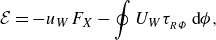 \begin{equation} \mathcal{E} = - {u_{W}} {F_{X}} - \oint {U_{W}} {\tau _{_{R\Phi }}} \; \textrm {d} \phi, \end{equation}
where
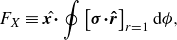 \begin{equation} {F_{X}} \equiv \hat {\boldsymbol{x \cdot }} \oint \left [ \boldsymbol{\sigma } \boldsymbol{\cdot \hat {r}}\right ]_{r=1} \textrm {d} \phi, \end{equation}
is the drag force exerted on the inner disk.
5.1. Pure translation
Solutions for flow around a disk in pure translation ( ${u_{W}}=1$
,
${u_{W}}=1$
, ${U_{W}}=0$
) with three different annular gaps,
${U_{W}}=0$
) with three different annular gaps, $\unicode{x1D6E5} =\ell -1$
, are shown in figure 10. For a sufficiently wide gap, the fluid plugs up further away from the inner cylinder, rendering the outer cylinder irrelevant and the flow equivalent to that around an isolated disk, as illustrated earlier in figure 1. Randolph & Houlsby (Reference Randolph and Houlsby1984) provided a slipline solution for the perfectly plastic version of this problem which is compared with the numerical solution (at finite
$\unicode{x1D6E5} =\ell -1$
, are shown in figure 10. For a sufficiently wide gap, the fluid plugs up further away from the inner cylinder, rendering the outer cylinder irrelevant and the flow equivalent to that around an isolated disk, as illustrated earlier in figure 1. Randolph & Houlsby (Reference Randolph and Houlsby1984) provided a slipline solution for the perfectly plastic version of this problem which is compared with the numerical solution (at finite $\textit{Bi}$
) in figure 10(a). The slipline field contains triangular checkerboards attached to the front and back of the disk, with semicircular fans positioned to either side; between the fans and checkerboards, the sliplines are involutes of the disk. As mentioned earlier, the velocity field across the checkerboards is consistent with solid-body motion, rendering these regions into serendipitous plugs in the numerical solution. The cores of the semicircular fans also solidify into residual plugs.
$\textit{Bi}$
) in figure 10(a). The slipline field contains triangular checkerboards attached to the front and back of the disk, with semicircular fans positioned to either side; between the fans and checkerboards, the sliplines are involutes of the disk. As mentioned earlier, the velocity field across the checkerboards is consistent with solid-body motion, rendering these regions into serendipitous plugs in the numerical solution. The cores of the semicircular fans also solidify into residual plugs.
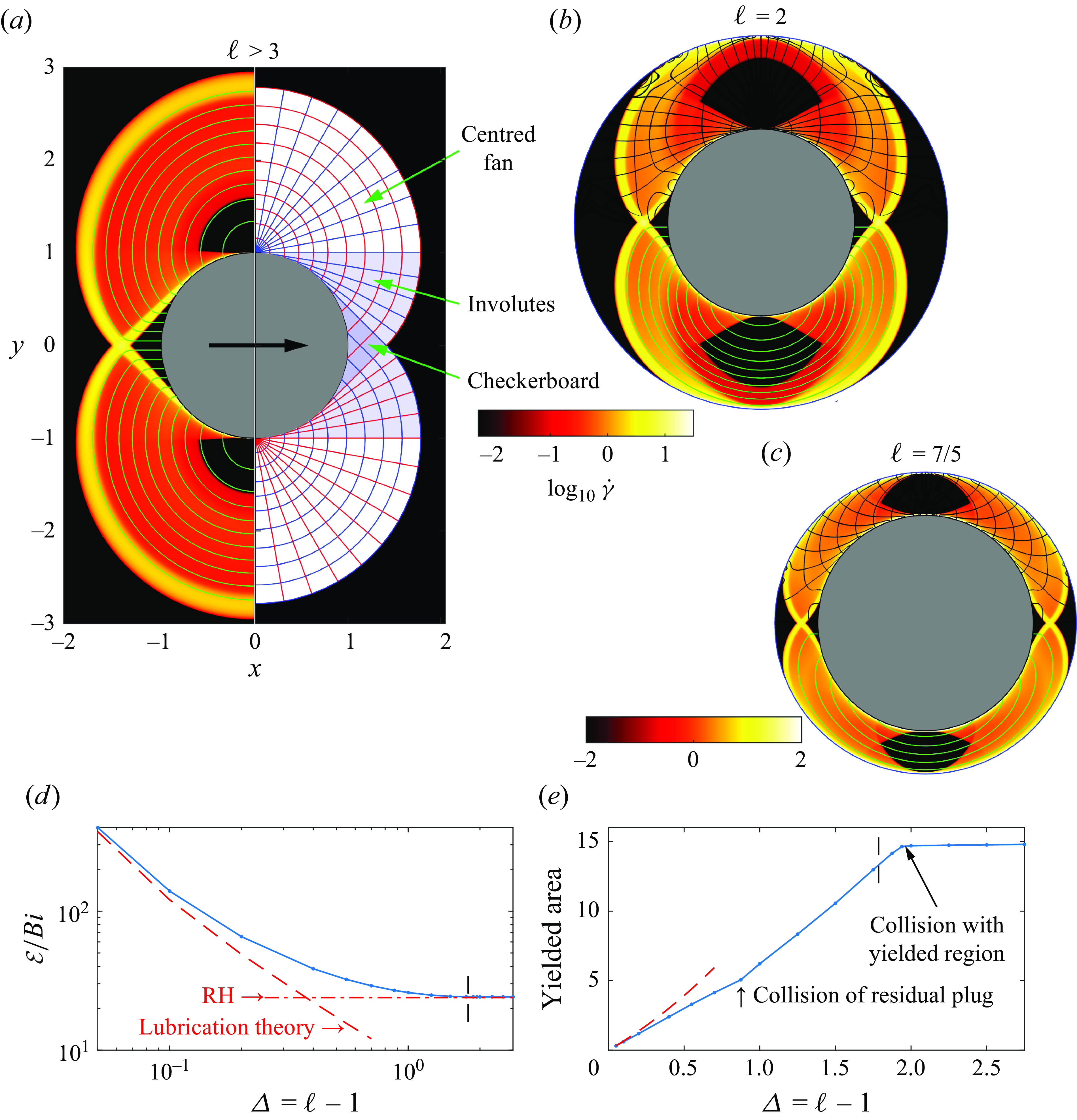
Figure 10. Translating cylinders for varying outer radius $\ell$
(as indicated), showing density maps of
$\ell$
(as indicated), showing density maps of $\log _{10}{\dot \gamma }$
along with sample streamlines (green). A selection of sliplines from Randolph & Houlsby’s solution are included in (a) (green lines), and from reconstructions using the numerical stress field in (b,c) (black lines). (d) Net dissipation rate
$\log _{10}{\dot \gamma }$
along with sample streamlines (green). A selection of sliplines from Randolph & Houlsby’s solution are included in (a) (green lines), and from reconstructions using the numerical stress field in (b,c) (black lines). (d) Net dissipation rate $\mathcal{E}/\textit{Bi}$
and (e) yielded area are plotted against
$\mathcal{E}/\textit{Bi}$
and (e) yielded area are plotted against $\unicode{x1D6E5} =\ell -1$
for a wider suite of computations. The (red) dashed lines display the predictions of lubrication theory (§ C.2); the dot-dashed line in (d) shows
$\unicode{x1D6E5} =\ell -1$
for a wider suite of computations. The (red) dashed lines display the predictions of lubrication theory (§ C.2); the dot-dashed line in (d) shows $\mathcal{E}/\textit{Bi}$
for Randolph & Houlsby’s solution (labelled RH). In (e), two flow patterns transitions are indicated: the values of
$\mathcal{E}/\textit{Bi}$
for Randolph & Houlsby’s solution (labelled RH). In (e), two flow patterns transitions are indicated: the values of $\unicode{x1D6E5}$
at which either the yielded region or the residual plug collides with the outer wall. The vertical dashed lines indicate the prediction for the former using Randolph & Houlsby’s solution.
$\unicode{x1D6E5}$
at which either the yielded region or the residual plug collides with the outer wall. The vertical dashed lines indicate the prediction for the former using Randolph & Houlsby’s solution. $\textit{Bi}=2048$
and
$\textit{Bi}=2048$
and $n=1$
.
$n=1$
.
Randolph & Houlsby’s slipline construction is analytical, and the net dissipation rate $\mathcal{E}$
can be calculated by hand along with the drag
$\mathcal{E}$
can be calculated by hand along with the drag $F_{X}$
and torque
$F_{X}$
and torque $T$
on the cylinder
$T$
on the cylinder
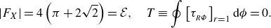 \begin{equation} |{F_{X}}| = 4 \left(\pi +2\sqrt {2} \right) = \mathcal{E}, \quad T \equiv \oint \left [ {\tau _{_{R\Phi }}} \right ]_{r=1} \textrm {d} \phi = 0. \end{equation}
Importantly, Randolph & Houlsby also demonstrate that one can find an acceptable stress field over the attached plugs and surrounding stationary plug; as already noted, the stress field is indeterminate over these regions, but to fully complete a slipline solution, one must show that there is an admissible stress over each plug that satisfies the force-balance equations (3.2) and yield condition ( ${\tau ^2_{_{\textit{XX}}}}+{\tau ^2_{_{YY}}}\lt \textit{Bi}^2$
).
${\tau ^2_{_{\textit{XX}}}}+{\tau ^2_{_{YY}}}\lt \textit{Bi}^2$
).
The other two solutions displayed in figure 10 indicate how the flow, and Randolph & Houlsby’s slipline field, becomes distorted when the outer boundary lies too close to the inner cylinder ( $\ell \lt 2+(1/4)\pi \approx 2.79$
for
$\ell \lt 2+(1/4)\pi \approx 2.79$
for $\textit{Bi}\to \infty$
). Other features remain, such as the residual plugs and the viscoplastic shear and boundary layers. Note that the slipline patterns reconstructed from the numerical solutions here are rather imprecise (especially in figure 10
b), which illustrates that construction of these characteristics can be delicate, particularly near non-plastic flow features (e.g. shear layers and rigid plugs).
$\textit{Bi}\to \infty$
). Other features remain, such as the residual plugs and the viscoplastic shear and boundary layers. Note that the slipline patterns reconstructed from the numerical solutions here are rather imprecise (especially in figure 10
b), which illustrates that construction of these characteristics can be delicate, particularly near non-plastic flow features (e.g. shear layers and rigid plugs).
The progression of the flow pattern as once proceeds from the wide-gap (Randolph–Houlsby) solution to the thin-gap limit is shown more quantitatively in figure 10(d,e). Here, net dissipation rates and yielded areas are presented for a wider suite of computations with varying $\ell$
. There are two second-order transitions in flow pattern present in this progression. The first transition arises when the yielded regions meet the shrinking outer cylinder, which occurs for
$\ell$
. There are two second-order transitions in flow pattern present in this progression. The first transition arises when the yielded regions meet the shrinking outer cylinder, which occurs for $\ell =2+ {\pi }/{4}$
according to Randolph & Houlsby’s slipline solution. The second arises only when
$\ell =2+ {\pi }/{4}$
according to Randolph & Houlsby’s slipline solution. The second arises only when $\textit{Bi}$
is finite, and corresponds to the collision of the outer wall with the residual plugs lying near the top and bottom of the disk. Both transitions are second order because slipline patterns exist to either side of the transitions that continuously connect to one another; no sudden jumps arise in pattern geometry, and no plugs break.
$\textit{Bi}$
is finite, and corresponds to the collision of the outer wall with the residual plugs lying near the top and bottom of the disk. Both transitions are second order because slipline patterns exist to either side of the transitions that continuously connect to one another; no sudden jumps arise in pattern geometry, and no plugs break.
5.2. The narrow-gap limit; annular squeeze flow
When the gap between the cylinders is narrow, $\ell -1=\unicode{x1D6E5} \ll 1$
, lubrication theory can be used to build solutions analytically. We illustrate this construction for the case of a uniformly translating inner disk (
$\ell -1=\unicode{x1D6E5} \ll 1$
, lubrication theory can be used to build solutions analytically. We illustrate this construction for the case of a uniformly translating inner disk ( ${u_{W}}=1$
,
${u_{W}}=1$
, ${U_{W}}=0$
); i.e. an annular squeeze-flow problem. Figure 11 presents numerical solutions in this limit, and a comparison with predictions from lubrication analysis, which is summarised in more detail in § C.2. Figure 10(e,g) also includes the corresponding predictions for the dissipation rate and plug area. The former is quoted in (C36), whereas the latter equals the area of the annulus because the plugs all become small in the thin-gap limit (the relevant Bingham number is
${U_{W}}=0$
); i.e. an annular squeeze-flow problem. Figure 11 presents numerical solutions in this limit, and a comparison with predictions from lubrication analysis, which is summarised in more detail in § C.2. Figure 10(e,g) also includes the corresponding predictions for the dissipation rate and plug area. The former is quoted in (C36), whereas the latter equals the area of the annulus because the plugs all become small in the thin-gap limit (the relevant Bingham number is $B=\unicode{x1D6E5} ^2\textit{Bi}$
, rather than
$B=\unicode{x1D6E5} ^2\textit{Bi}$
, rather than $\textit{Bi}$
, implying flow becomes effectively Newtonian for
$\textit{Bi}$
, implying flow becomes effectively Newtonian for $\unicode{x1D6E5} \to 0$
at fixed
$\unicode{x1D6E5} \to 0$
at fixed $\textit{Bi}$
).
$\textit{Bi}$
).
The density plots of the strain-rate invariant in panel (a) illustrate how the lubrication flow adopts a distinctive character in which a relatively weakly sheared region occupies the centre of the gap. This plug-like central flow is the thin-gap relative of the nearly plastic flow region in wider annuli (cf. figures 1 and 10), and is buffered from the walls by layers of stronger shear (which are the cousins of the boundary layers in figure 1). This layered flow pattern is the hallmark of the lubrication limit (§ C.2). Because the central region is not fully rigid, common practice is to refer it as a ‘pseudo-plug’, following Walton & Bittleston (Reference Walton and Bittleston1991). Earlier work has sometimes incorrectly identified the pseudo-plug as a true plug, and then falsely claimed an inconsistency in the lubrication analysis because of the weaker shear that remains present (the fallacy of the lubrication paradox).
The solution in figure 11, with $\unicode{x1D6E5} =1/5$
, is not particularly close to the narrow-gap limit. Consequently, there are noticeable discrepancies with the predictions of lubrication theory in the velocity profiles displayed in figure 11(b,c). The numerical solution matches the asymptotic predictions more closely for narrower gaps, as illustrated in figure 12 which presents numerical solutions for
$\unicode{x1D6E5} =1/5$
, is not particularly close to the narrow-gap limit. Consequently, there are noticeable discrepancies with the predictions of lubrication theory in the velocity profiles displayed in figure 11(b,c). The numerical solution matches the asymptotic predictions more closely for narrower gaps, as illustrated in figure 12 which presents numerical solutions for $\unicode{x1D6E5} ={1}/{20}$
. In this example, the main disagreements arise around the border between the pseudo-plug and the more strongly sheared layers. In fact, the lubrication velocity profile here can be further improved by smoothing out the splice between the two regions over a narrow intervening transition zone (Walton & Bittleston Reference Walton and Bittleston1991; Putz et al. Reference Putz, Burghelea, Frigaard and Martinez2008; Muravleva Reference Muravleva2015).
$\unicode{x1D6E5} ={1}/{20}$
. In this example, the main disagreements arise around the border between the pseudo-plug and the more strongly sheared layers. In fact, the lubrication velocity profile here can be further improved by smoothing out the splice between the two regions over a narrow intervening transition zone (Walton & Bittleston Reference Walton and Bittleston1991; Putz et al. Reference Putz, Burghelea, Frigaard and Martinez2008; Muravleva Reference Muravleva2015).
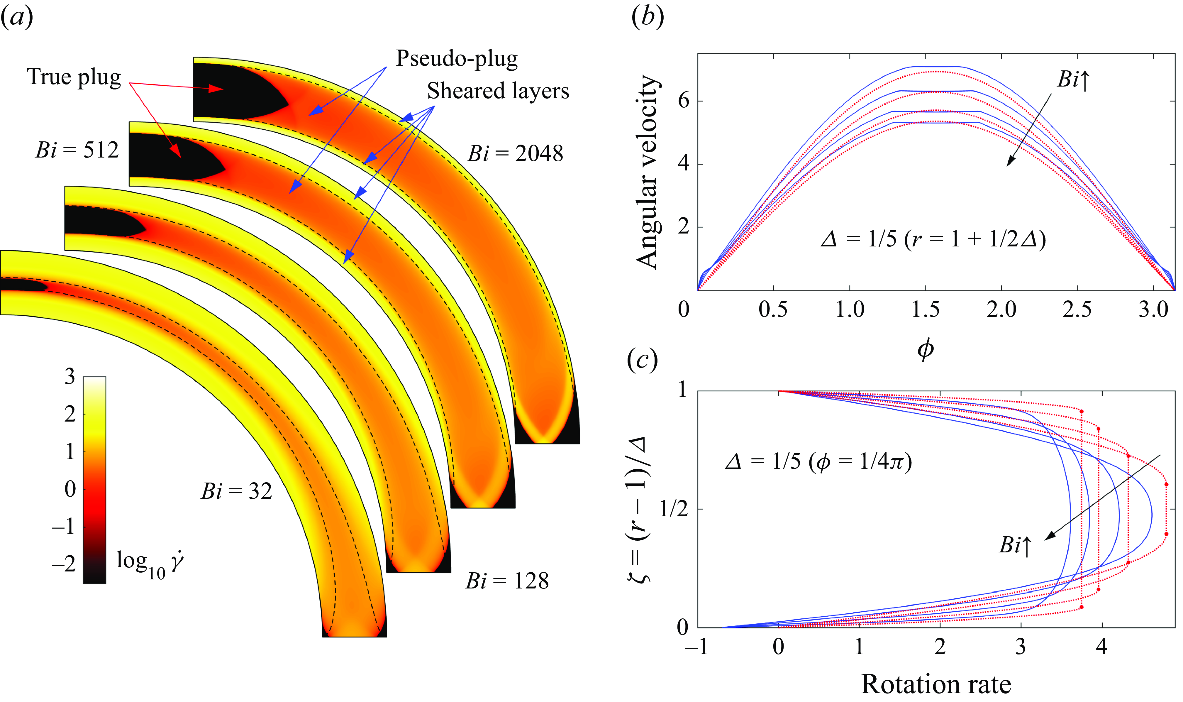
Figure 11. Squeeze flow in the narrow gap (of radial width $\unicode{x1D6E5}$
) between two cylinders, with the inner cylinder moving to the right at unit speed and the outer cylinder stationary. (a–c) Solutions for
$\unicode{x1D6E5}$
) between two cylinders, with the inner cylinder moving to the right at unit speed and the outer cylinder stationary. (a–c) Solutions for $\unicode{x1D6E5} = 1/5$
: (a) density plots of
$\unicode{x1D6E5} = 1/5$
: (a) density plots of $\log _{10}{\dot \gamma }$
for the values of
$\log _{10}{\dot \gamma }$
for the values of $\textit{Bi}$
indicated in each quadrant; (b) cuts through the angular velocity along the midline
$\textit{Bi}$
indicated in each quadrant; (b) cuts through the angular velocity along the midline $r=1+(1/2)\unicode{x1D6E5}$
(blue) are compared with the pseudo-plug velocity (C34) predicted by lubrication theory (red dashed); (c) cuts from the rotation rate at
$r=1+(1/2)\unicode{x1D6E5}$
(blue) are compared with the pseudo-plug velocity (C34) predicted by lubrication theory (red dashed); (c) cuts from the rotation rate at $\phi =(1/4)\pi$
(blue) are compared against the asymptotic velocity profile (C30) (red dotted). The dashed lines in (a) and the dots in (c) indicate the predicted fake yield surfaces
$\phi =(1/4)\pi$
(blue) are compared against the asymptotic velocity profile (C30) (red dotted). The dashed lines in (a) and the dots in (c) indicate the predicted fake yield surfaces $r=1+Y$
and
$r=1+Y$
and $r=1+\unicode{x1D6E5} -Y$
from (C33).
$r=1+\unicode{x1D6E5} -Y$
from (C33).
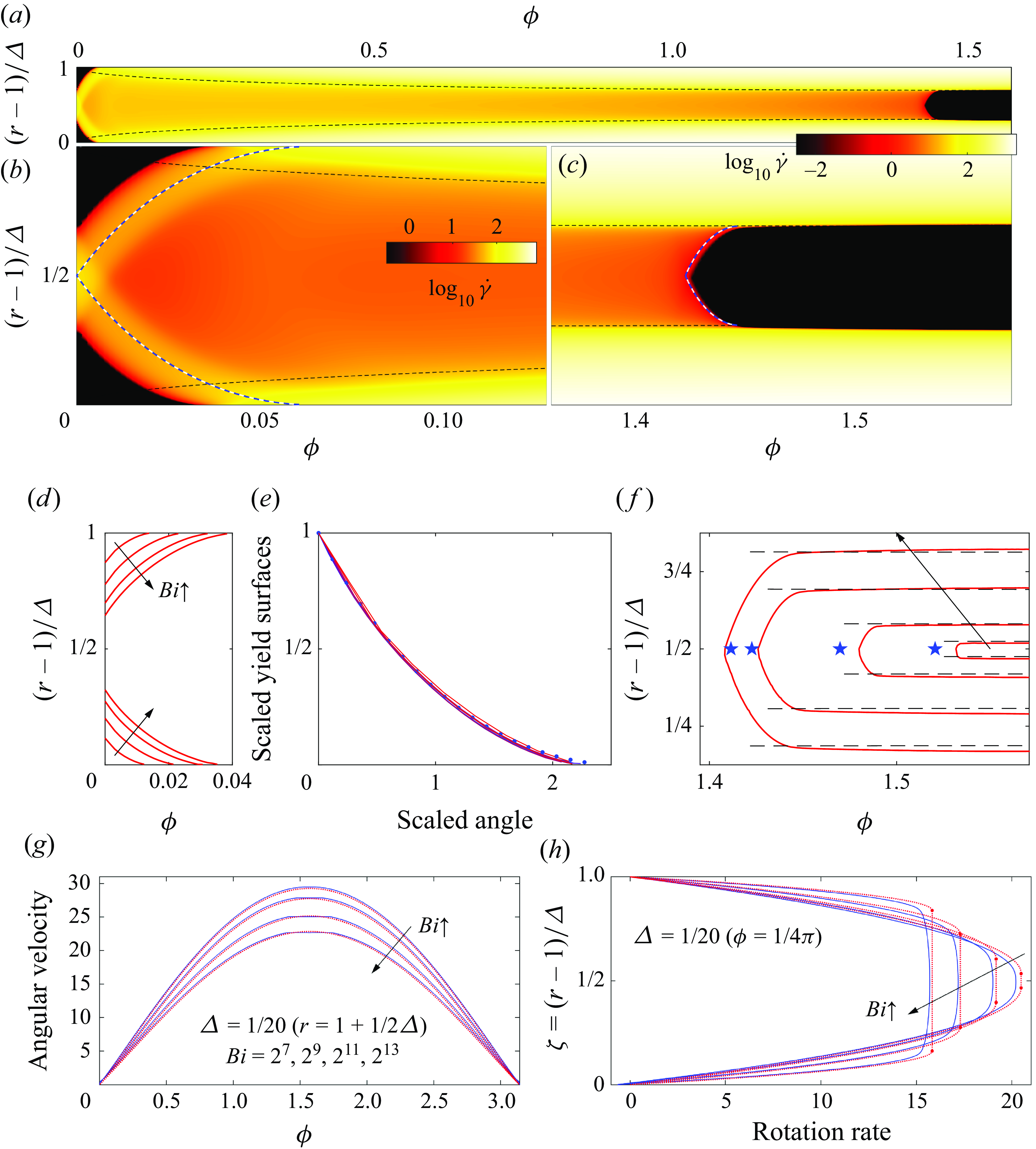
Figure 12. The thin-gap squeeze-flow solution for $\unicode{x1D6E5} = {1}/{20}$
(
$\unicode{x1D6E5} = {1}/{20}$
( $n=1$
). Density plots of
$n=1$
). Density plots of $\log _{10}{\dot \gamma }$
are plotted in panels (a–c) for
$\log _{10}{\dot \gamma }$
are plotted in panels (a–c) for $\textit{Bi}=2048$
: (a) shows the entire solution over
$\textit{Bi}=2048$
: (a) shows the entire solution over $0\lt \phi \lt {1}/{2}\pi$
; (b) and (c) show magnifications near
$0\lt \phi \lt {1}/{2}\pi$
; (b) and (c) show magnifications near $\phi =0$
and
$\phi =0$
and ${1}/{2}\pi$
, respectively. The black dashed lines show the fake yield surfaces,
${1}/{2}\pi$
, respectively. The black dashed lines show the fake yield surfaces, $r=1+Y$
and
$r=1+Y$
and $r=1+\unicode{x1D6E5} -Y$
, from (C33). The blue and white dashed lines show Prandtl’s cycloids (3.19), intersecting either
$r=1+\unicode{x1D6E5} -Y$
, from (C33). The blue and white dashed lines show Prandtl’s cycloids (3.19), intersecting either $\theta =0$
or the predicted edge of true plug at
$\theta =0$
or the predicted edge of true plug at $\phi ={1}/{2}\pi$
. Panels (d–h) add further solutions with
$\phi ={1}/{2}\pi$
. Panels (d–h) add further solutions with $\textit{Bi}=128$
,
$\textit{Bi}=128$
, $512$
,
$512$
, $2048$
and
$2048$
and $8096$
. The plug borders for solutions are plotted (in red) in (d) and (f). In (e), the yield surfaces near
$8096$
. The plug borders for solutions are plotted (in red) in (d) and (f). In (e), the yield surfaces near $\phi =0$
are scaled, using
$\phi =0$
are scaled, using $[r(\phi )-1]/[r(0)-1]$
(for the lower) or
$[r(\phi )-1]/[r(0)-1]$
(for the lower) or $[1+\unicode{x1D6E5} -r(\phi )]/[1+\unicode{x1D6E5} -r(0)]$
(for the upper), then replotted against
$[1+\unicode{x1D6E5} -r(\phi )]/[1+\unicode{x1D6E5} -r(0)]$
(for the upper), then replotted against $\phi /[r(0)-1]$
or
$\phi /[r(0)-1]$
or $\phi /[1+\unicode{x1D6E5} -r(0)]$
. The blue dots show Prandtl’s cycloid. In (e), the prediction (C74) of Appendix C.3 for the edges of the plugs at
$\phi /[1+\unicode{x1D6E5} -r(0)]$
. The blue dots show Prandtl’s cycloid. In (e), the prediction (C74) of Appendix C.3 for the edges of the plugs at $\phi = {1}/{2}\pi$
are indicated by (blue) stars, and the dashed lines indicate the radial borders given by (C33). In (g) and (h), cuts of the angular velocity along the midline (
$\phi = {1}/{2}\pi$
are indicated by (blue) stars, and the dashed lines indicate the radial borders given by (C33). In (g) and (h), cuts of the angular velocity along the midline ( $r=1+(1/2) \unicode{x1D6E5}$
) and of the rotation rate at
$r=1+(1/2) \unicode{x1D6E5}$
) and of the rotation rate at $\phi =(1/4)\pi$
(blue lines) are compared with the predictions in (C30) and (C34) (red dotted lines). The (red) dots in (h) show the predicted fake yield surfaces from (C33).
$\phi =(1/4)\pi$
(blue lines) are compared with the predictions in (C30) and (C34) (red dotted lines). The (red) dots in (h) show the predicted fake yield surfaces from (C33).
More awkwardly, lubrication theory also predicts that the pseudo-plug (the weakly sheared central region) persists all the way around the annulus. The numerical solutions, however, display plugs attached to the walls near $\phi =0$
and
$\phi =0$
and $\pi$
, and true plugs embedded within the pseudo-plug near
$\pi$
, and true plugs embedded within the pseudo-plug near $\phi =\pm (1/2)\pi$
. These features are not captured by leading-order lubrication analysis (§ C.2), primarily because their angular scale is too small. Despite this, their presence can be detected in the details of that analysis.
$\phi =\pm (1/2)\pi$
. These features are not captured by leading-order lubrication analysis (§ C.2), primarily because their angular scale is too small. Despite this, their presence can be detected in the details of that analysis.
First, the attached plugs near $\phi =0$
and
$\phi =0$
and $\pi$
can be anticipated because the lubrication analysis predicts that the pseudo-plug expands to fill the entire gap if
$\pi$
can be anticipated because the lubrication analysis predicts that the pseudo-plug expands to fill the entire gap if $\sin \phi =0$
(see (C33) and figures 11
a and 12
a). But this further implies that the entire gap then truly plugs up. Evidently, away from the asymptotic limit, such unyielded points broaden into the attached plugs over an angular scale comparable to the gap.
$\sin \phi =0$
(see (C33) and figures 11
a and 12
a). But this further implies that the entire gap then truly plugs up. Evidently, away from the asymptotic limit, such unyielded points broaden into the attached plugs over an angular scale comparable to the gap.
Second, the lubrication analysis fails to recover the true plugs at $\phi =\pm (1/2)\pi$
because it implicitly assumes that the pseudo-plug solution is always weakly sheared. But, at
$\phi =\pm (1/2)\pi$
because it implicitly assumes that the pseudo-plug solution is always weakly sheared. But, at $\phi =\pm (1/2)\pi$
, the angular velocity of the pseudo-plug reaches a maximum (see figures 11
b and 12
g) and the shear in the pseudo-plug locally vanishes. This opens up the possibility of a different asymptotic solution in which a true plug arises at the centre of the gap. One can construct this solution by adapting a method presented by Walton & Bittleston (who considered axial viscoplastic flow down an eccentric annular duct; see also Frigaard & Ryan (Reference Frigaard and Ryan2004); Putz et al. (Reference Putz, Burghelea, Frigaard and Martinez2008); Liu et al. (Reference Liu, Balmforth and Hormozi2019); Balmforth et al. (Reference Balmforth, Craster and Hewitt2021)). This higher-order extension of the lubrication theory is provided in Appendix C.3, and predicts embedded plugs with angular borders that are indicated by stars in figure 12(f).
$\phi =\pm (1/2)\pi$
, the angular velocity of the pseudo-plug reaches a maximum (see figures 11
b and 12
g) and the shear in the pseudo-plug locally vanishes. This opens up the possibility of a different asymptotic solution in which a true plug arises at the centre of the gap. One can construct this solution by adapting a method presented by Walton & Bittleston (who considered axial viscoplastic flow down an eccentric annular duct; see also Frigaard & Ryan (Reference Frigaard and Ryan2004); Putz et al. (Reference Putz, Burghelea, Frigaard and Martinez2008); Liu et al. (Reference Liu, Balmforth and Hormozi2019); Balmforth et al. (Reference Balmforth, Craster and Hewitt2021)). This higher-order extension of the lubrication theory is provided in Appendix C.3, and predicts embedded plugs with angular borders that are indicated by stars in figure 12(f).
The higher-order lubrication analysis assumes that the angular length of the plug is relatively small, but not as small as the gap. Consequently, the plug is predicted to end at a single angular position. The numerical solutions, however, display yield surfaces with a definite shape, albeit of the scale of the gap (see figures 11 and 12), similar to the attached plugs. In fact, both yield surfaces closely follow Prandtl cycloidal sliplines, as illustrated in figure 12(b,c).
We rationalise this observation by first noting that on the scale of the narrow gap, the walls appear straight and parallel with a nearly constant pressure gradient, $\partial P / \partial s=-\Gamma \textit{Bi}$
. At
$\partial P / \partial s=-\Gamma \textit{Bi}$
. At $\phi =0$
, we have
$\phi =0$
, we have $Y\to 0$
or
$Y\to 0$
or $\Gamma =2 \Delta ^{-1}$
, whereas
$\Gamma =2 \Delta ^{-1}$
, whereas $\Gamma = [(1/2)\unicode{x1D6E5} -Y({1}/{2}\pi )]^{-1}$
near
$\Gamma = [(1/2)\unicode{x1D6E5} -Y({1}/{2}\pi )]^{-1}$
near $\phi = {1}/{2}\pi$
. Inserting these two options into (3.19) gives the sliplines also plotted, choosing either
$\phi = {1}/{2}\pi$
. Inserting these two options into (3.19) gives the sliplines also plotted, choosing either $x_0=0$
or the location of the edge of the plug near
$x_0=0$
or the location of the edge of the plug near $\phi =(1/2)\pi$
predicted by (C74).
$\phi =(1/2)\pi$
predicted by (C74).
To reinforce this point, we exploit the scale invariant form of the cycloid noted in § 3.4.2 to collapse all the yield surfaces measured from the numerical solutions near $\phi =0$
: for the lower yield surfaces, we scale
$\phi =0$
: for the lower yield surfaces, we scale $r(\phi )-1$
and
$r(\phi )-1$
and $\phi$
by
$\phi$
by $r(0)-1$
, then scale
$r(0)-1$
, then scale $1+\unicode{x1D6E5} -r(\phi )$
and
$1+\unicode{x1D6E5} -r(\phi )$
and $\phi$
by
$\phi$
by $1+\unicode{x1D6E5} -r(0)$
for the upper yield surface. As shown by figure 12(e), this scaling successfully collapses the observed yield surfaces onto Prandtl’s cycloid.
$1+\unicode{x1D6E5} -r(0)$
for the upper yield surface. As shown by figure 12(e), this scaling successfully collapses the observed yield surfaces onto Prandtl’s cycloid.
Note that the floating plugs at $\phi =\pm (1/2)\pi$
correspond to the small-gap limit of the residual plugs at the core of the semi-circular fans of Randolph & Houlsby’s slipline field (figures 1
a,b and 10
a). Indeed, the former also disappear as
$\phi =\pm (1/2)\pi$
correspond to the small-gap limit of the residual plugs at the core of the semi-circular fans of Randolph & Houlsby’s slipline field (figures 1
a,b and 10
a). Indeed, the former also disappear as $\textit{Bi}\to \infty$
(
$\textit{Bi}\to \infty$
( $Y\to {1}/{2}$
in this limit; see (C74)). On the other hand, the plugs attached to the inner cylinder at
$Y\to {1}/{2}$
in this limit; see (C74)). On the other hand, the plugs attached to the inner cylinder at $\phi =0$
and
$\phi =0$
and $\phi =\pi$
are the remnants of the triangular plugs attached to the front and back of the disk in figure 1 (and are no longer serendipitous). The ambient plug that surrounds and cloaks the outer cylinder in figure 1 becomes compressed into the plugs attached to the outer cylinder at
$\phi =\pi$
are the remnants of the triangular plugs attached to the front and back of the disk in figure 1 (and are no longer serendipitous). The ambient plug that surrounds and cloaks the outer cylinder in figure 1 becomes compressed into the plugs attached to the outer cylinder at $\phi =0$
and
$\phi =0$
and $\phi =\pi$
.
$\phi =\pi$
.
5.3. Translation with rotation
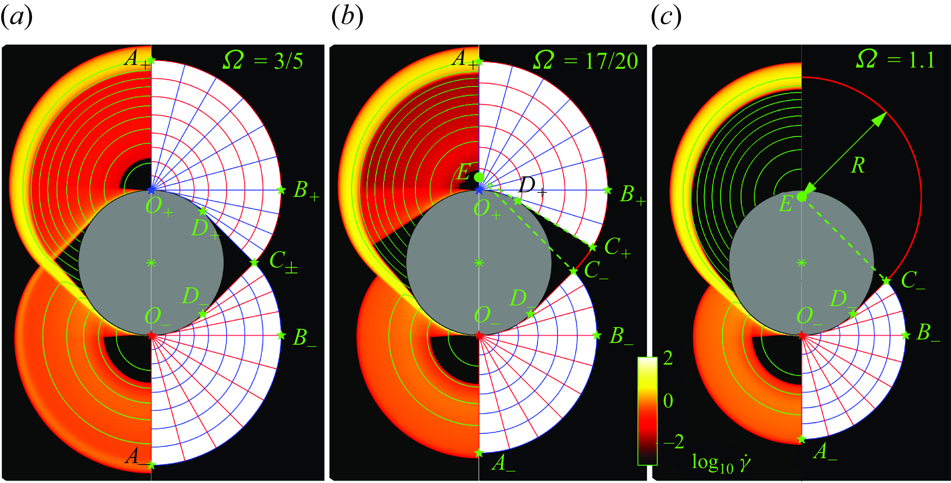
Figure 13. Translating and rotating cylinders for varying rotation speed $\Omega$
(as indicated; translation speed in positive
$\Omega$
(as indicated; translation speed in positive $x$
direction is again scaled to unity). On the left of each plot, we display a density map of
$x$
direction is again scaled to unity). On the left of each plot, we display a density map of $\log _{10}{\dot \gamma }$
for the numerical solution along with sample streamlines. On the right, we show the corresponding slipline solution, with various important points indicated. Plugs are shaded black, and the
$\log _{10}{\dot \gamma }$
for the numerical solution along with sample streamlines. On the right, we show the corresponding slipline solution, with various important points indicated. Plugs are shaded black, and the $\alpha$
(
$\alpha$
( $\beta$
) lines are plotted as red (blue) lines.
$\beta$
) lines are plotted as red (blue) lines.
Returning again to the limit in which the outer cylinder is sufficiently distant that it does not affect the flow, we now allow the inner cylinder to rotate as well as translate (Hewitt & Balmforth Reference Hewitt and Balmforth2018). Solutions in the plastic limit are illustrated in figure 13. Surprisingly, although one expects that rotation breaks sideways symmetry (up-down in the figures), the stress field remains symmetrical and equivalent to that of Randolph & Houlsby as long as $\Omega \lt ({1}/{\sqrt 2})$
(figure 13
a). This feature becomes reflected in the drag and torque, which remain at the values given in (5.4) to leading order; see figure 14. Nevertheless, the velocity field is asymmetrical, as illustrated in figure 13(a). This solution demonstrates how it is possible for an asymmetrical velocity field to be consistent with a symmetrical stress field in the plastic limit, since only the orientation of the strain-rate tensor needs to be symmetrical in (3.14), not the invariant
$\Omega \lt ({1}/{\sqrt 2})$
(figure 13
a). This feature becomes reflected in the drag and torque, which remain at the values given in (5.4) to leading order; see figure 14. Nevertheless, the velocity field is asymmetrical, as illustrated in figure 13(a). This solution demonstrates how it is possible for an asymmetrical velocity field to be consistent with a symmetrical stress field in the plastic limit, since only the orientation of the strain-rate tensor needs to be symmetrical in (3.14), not the invariant $\dot \gamma$
itself.
$\dot \gamma$
itself.
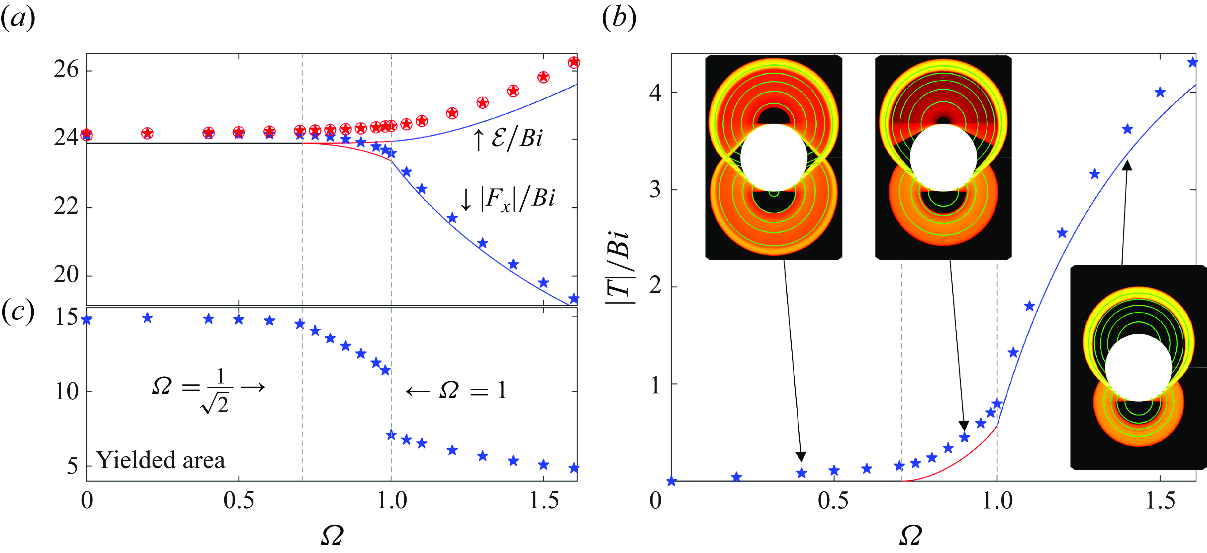
Figure 14. (a) Forces $|{F_{X}}|$
and dissipation rates
$|{F_{X}}|$
and dissipation rates $\mathcal{E}$
, scaled by
$\mathcal{E}$
, scaled by $\textit{Bi}$
, plotted against
$\textit{Bi}$
, plotted against $\Omega$
for translating and rotating cylinders. In (b,c) we show the corresponding torques
$\Omega$
for translating and rotating cylinders. In (b,c) we show the corresponding torques $T/\textit{Bi}$
and yielded areas, respectively. The stars indicate data taken from numerical solutions. The black, red and blue lines show the slipline predictions for the three different flow patterns, which are illustrated in the insets to (b) (density maps of
$T/\textit{Bi}$
and yielded areas, respectively. The stars indicate data taken from numerical solutions. The black, red and blue lines show the slipline predictions for the three different flow patterns, which are illustrated in the insets to (b) (density maps of $\log _{10}{\dot \gamma }$
) and shown in more detail in figure 13 (with the same colour scale). In (a), the red stars show
$\log _{10}{\dot \gamma }$
) and shown in more detail in figure 13 (with the same colour scale). In (a), the red stars show $\mathcal{E}$
, as computed from the velocity field, and the red circles indicate
$\mathcal{E}$
, as computed from the velocity field, and the red circles indicate $|{F_{X}}+\Omega T|$
.
$|{F_{X}}+\Omega T|$
.
When $\Omega$
reaches
$\Omega$
reaches $({1}/{\sqrt 2})$
, the asymmetrical velocity field is no longer able to remain consistent with the symmetrical stress field. This arises because the (anti-clockwise) tangential velocity along the section
$({1}/{\sqrt 2})$
, the asymmetrical velocity field is no longer able to remain consistent with the symmetrical stress field. This arises because the (anti-clockwise) tangential velocity along the section $O_+ D_+$
of the disk is
$O_+ D_+$
of the disk is $\Omega -\sin \phi$
,
$\Omega -\sin \phi$
, $(1/4)\pi \lt \phi \lt (1/2)\pi$
, whereas the plastic region on the other side of the wall boundary layer has zero angular velocity. Thus, between the plastic region and disk there is a tangential slip velocity of
$(1/4)\pi \lt \phi \lt (1/2)\pi$
, whereas the plastic region on the other side of the wall boundary layer has zero angular velocity. Thus, between the plastic region and disk there is a tangential slip velocity of $\sin \phi -\Omega$
, which must have the same sign as the local shear stress,
$\sin \phi -\Omega$
, which must have the same sign as the local shear stress, ${\tau _{_{R\Phi }}}=-\textit{Bi}$
. This can only be true if
${\tau _{_{R\Phi }}}=-\textit{Bi}$
. This can only be true if $\Omega \lt ({1}/{\sqrt {2}})$
.
$\Omega \lt ({1}/{\sqrt {2}})$
.
For higher rotation rates, the stress field necessarily deviates from the Randolph & Houlbsy form and becomes asymmetrical, as seen in figure 13(b). In particular, the rightmost involutes leaving the front of the cylinder no longer meet at $(x,y)=(\sqrt 2,0)$
. Instead, a gap opens, with the attached plug separated from the surrounding ambient plug by the circular slip surface
$(x,y)=(\sqrt 2,0)$
. Instead, a gap opens, with the attached plug separated from the surrounding ambient plug by the circular slip surface $C_-C_+$
. This arc is centred at point
$C_-C_+$
. This arc is centred at point $E$
, which is the centre of rotation of the combined velocity field of the cylinder,
$E$
, which is the centre of rotation of the combined velocity field of the cylinder, $(1,0)+\Omega (-y,x) = \Omega (y_{\Omega }-y,x)$
with
$(1,0)+\Omega (-y,x) = \Omega (y_{\Omega }-y,x)$
with $y_{\Omega }=\Omega ^{-1}$
.
$y_{\Omega }=\Omega ^{-1}$
.
The arc $C_-C_+$
widens as
$C_-C_+$
widens as $\Omega$
is increased still further. Eventually, for
$\Omega$
is increased still further. Eventually, for $\Omega =1$
, the rotation centre
$\Omega =1$
, the rotation centre $E$
reaches the centre of the fan
$E$
reaches the centre of the fan $O_+$
and the attached plug meets the semi-circular fan on that side of the disk. At this stage, the entire upper fan plugs up, as illustrated in figure 13(c). This third slipline pattern was constructed previously by Hewitt & Balmforth (Reference Hewitt and Balmforth2018). As highlighted by the area of the yielded region plotted in figure 14(c), the first switch in flow pattern at
$O_+$
and the attached plug meets the semi-circular fan on that side of the disk. At this stage, the entire upper fan plugs up, as illustrated in figure 13(c). This third slipline pattern was constructed previously by Hewitt & Balmforth (Reference Hewitt and Balmforth2018). As highlighted by the area of the yielded region plotted in figure 14(c), the first switch in flow pattern at $\Omega =1/\sqrt 2$
is second order because the intersecting slipline fields are compatible. The second switch at
$\Omega =1/\sqrt 2$
is second order because the intersecting slipline fields are compatible. The second switch at $\Omega =1$
is first order, because the rotating plug of the last pattern breaks.
$\Omega =1$
is first order, because the rotating plug of the last pattern breaks.
The drag, torque and dissipation rate can be calculated analytically for all of the three slipline patterns in figure 13 (see § B.3). In each case, $\mathcal{E} = |{F_{X}}|+|\Omega T|$
. The predictions are included in figure 14. Note that the torque calculated numerically for solutions with
$\mathcal{E} = |{F_{X}}|+|\Omega T|$
. The predictions are included in figure 14. Note that the torque calculated numerically for solutions with $\textit{Bi}=2048$
does not vanish for
$\textit{Bi}=2048$
does not vanish for $\Omega \lt ({1}/{\sqrt 2})$
because of a residual viscous torque stemming from the asymmetrical viscoplastic boundary and shear layers. For
$\Omega \lt ({1}/{\sqrt 2})$
because of a residual viscous torque stemming from the asymmetrical viscoplastic boundary and shear layers. For $\textit{Bi}\to \infty$
, however, the first slipline pattern (rather surprisingly) implies that a translating disk can rotate at a rate
$\textit{Bi}\to \infty$
, however, the first slipline pattern (rather surprisingly) implies that a translating disk can rotate at a rate $0\lt \Omega \lt ({1}/{\sqrt 2})$
without requiring any torque or incurring any additional dissipation beyond that expended for the non-rotating disk.
$0\lt \Omega \lt ({1}/{\sqrt 2})$
without requiring any torque or incurring any additional dissipation beyond that expended for the non-rotating disk.
Strictly speaking, as noted earlier, to establish that the slipline patterns in figure 13 are the exact solutions in the plastic limit one must further demonstrate that there is an acceptable stress field over each of the plugs. Randolph & Houlsby perform this construction for $\Omega =0$
, but none has been provided for the asymmetrical or rotating plugs of figure 13(b,c). Following Hewitt & Balmforth (Reference Hewitt and Balmforth2018) and § B.3, one can establish there are matching velocity and stress fields elsewhere which satisfy force balance, the constitutive law and boundary conditions. Hence, except for the extension of the stress field into the plugs, the extremum principles imply that
$\Omega =0$
, but none has been provided for the asymmetrical or rotating plugs of figure 13(b,c). Following Hewitt & Balmforth (Reference Hewitt and Balmforth2018) and § B.3, one can establish there are matching velocity and stress fields elsewhere which satisfy force balance, the constitutive law and boundary conditions. Hence, except for the extension of the stress field into the plugs, the extremum principles imply that $\mathcal{E} = |{F_{X}}|+|\Omega T|$
and the solutions are exact. That said, the numerical solutions provide evidence that admissible stress fields can be found for the plugs. Therefore, the slipline patterns do not only provide bounds on the net drag or dissipation rate, as sometimes they are constructed to do, but are the true solutions. Nor is it strictly necessarily to compute both
$\mathcal{E} = |{F_{X}}|+|\Omega T|$
and the solutions are exact. That said, the numerical solutions provide evidence that admissible stress fields can be found for the plugs. Therefore, the slipline patterns do not only provide bounds on the net drag or dissipation rate, as sometimes they are constructed to do, but are the true solutions. Nor is it strictly necessarily to compute both $\mathcal{E}$
and
$\mathcal{E}$
and $|{F_{X}}|+|\Omega T|$
independently and verify they are equal (they must be if all is consistent).
$|{F_{X}}|+|\Omega T|$
independently and verify they are equal (they must be if all is consistent).
5.4. Squirmers
The two examples shown in figure 10(a) and 13(a) repeat the possibility for two solutions to possess the same stress field but different velocity fields in the plastic limit. A third example is shown in figure 15(a,c), which corresponds to an idealised model of a circular microswimmer that ‘squirms’ through fluid by activating a tangential surface motion (Lighthill Reference Lighthill1975). More specifically, we consider domains for which the outer boundary $r=\ell$
is sufficiently far away that it is hidden by the surrounding plug, and, in (5.1), we take
$r=\ell$
is sufficiently far away that it is hidden by the surrounding plug, and, in (5.1), we take ${U_{W}}(\phi )=\phi (\pi -|\phi |)$
for
${U_{W}}(\phi )=\phi (\pi -|\phi |)$
for $-\pi \lt \phi \lt \pi$
(sinusoidal surface velocities were considered by Supekar et al. (Reference Supekar, Hewitt and Balmforth2020)). The (dimensionless) translation speed
$-\pi \lt \phi \lt \pi$
(sinusoidal surface velocities were considered by Supekar et al. (Reference Supekar, Hewitt and Balmforth2020)). The (dimensionless) translation speed $u_{W}$
is now a parameter of the problem, although for a genuine self-propelled squirmer,
$u_{W}$
is now a parameter of the problem, although for a genuine self-propelled squirmer, $u_{W}$
must be selected by demanding that no net forces are exerted on the inner disk (see below).
$u_{W}$
must be selected by demanding that no net forces are exerted on the inner disk (see below).
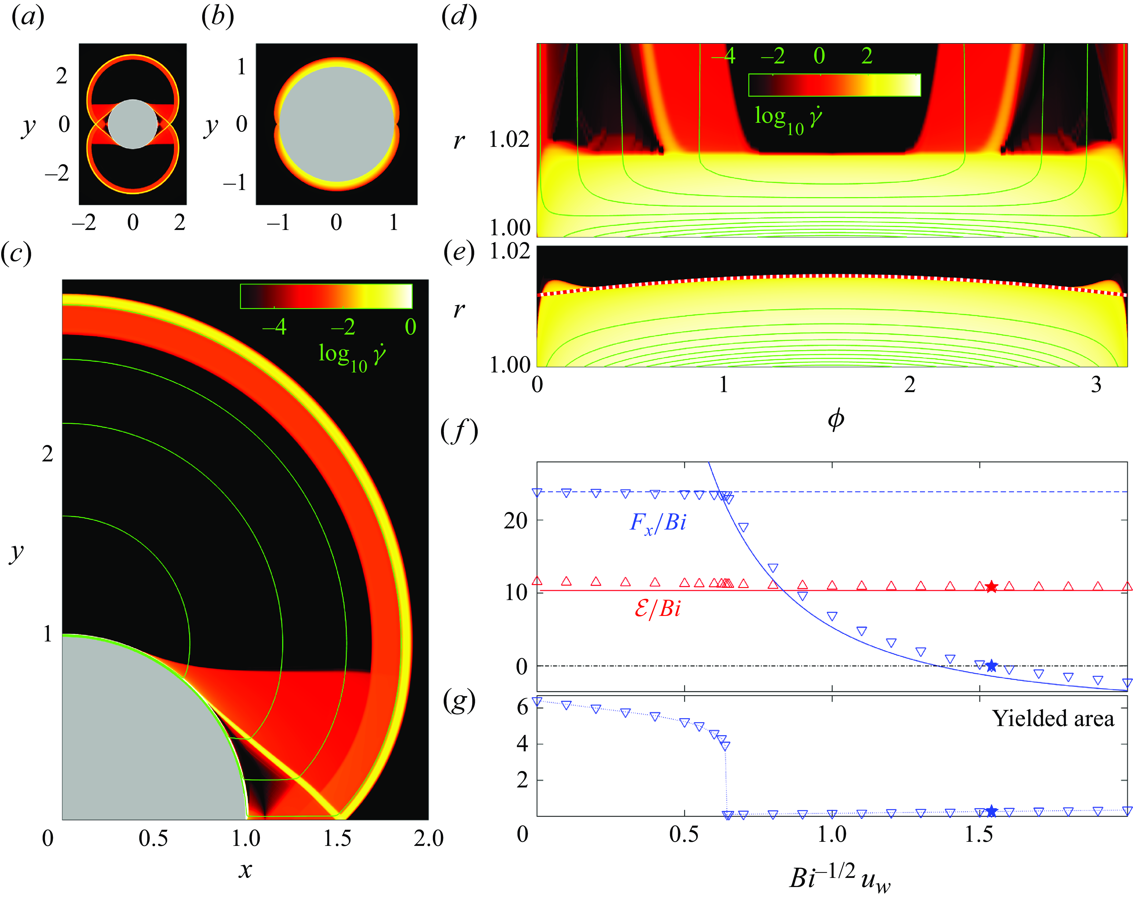
Figure 15. Model squirmers with a surface angular velocity ${U_{W}}(\phi )=\phi (\pi -|\phi |)$
for
${U_{W}}(\phi )=\phi (\pi -|\phi |)$
for $-\pi \lt \phi \lt \pi$
, and
$-\pi \lt \phi \lt \pi$
, and $\textit{Bi}=2048$
(
$\textit{Bi}=2048$
( $n=1$
). In (a), the (logarithmic) strain rate is plotted for a Randolph & Houlsby-like solution with a translation speed of
$n=1$
). In (a), the (logarithmic) strain rate is plotted for a Randolph & Houlsby-like solution with a translation speed of ${u_{W}}=0.4\textit{Bi}^{-1/2}$
; a boundary-layer solution with
${u_{W}}=0.4\textit{Bi}^{-1/2}$
; a boundary-layer solution with ${u_{W}}=5\textit{Bi}^{-1/2}$
is presented in (b). A magnified view of the first solution in the first quadrant is shown in (c), along with sample streamlines (green). The boundary layer against the squirmer is shown in more detail in (d). A corresponding plot for another boundary-layered solution with
${u_{W}}=5\textit{Bi}^{-1/2}$
is presented in (b). A magnified view of the first solution in the first quadrant is shown in (c), along with sample streamlines (green). The boundary layer against the squirmer is shown in more detail in (d). A corresponding plot for another boundary-layered solution with ${u_{W}}=0.7\textit{Bi}^{-1/2}$
is presented in (e) (the colour scale is the same as for (d)); the dotted line shows the prediction (C23) for the boundary-layer width. A suite of computations with varying
${u_{W}}=0.7\textit{Bi}^{-1/2}$
is presented in (e) (the colour scale is the same as for (d)); the dotted line shows the prediction (C23) for the boundary-layer width. A suite of computations with varying $\textit{Bi}^{1/2}{u_{W}}$
are presented in (f,g). Plotted are (f) the drag force
$\textit{Bi}^{1/2}{u_{W}}$
are presented in (f,g). Plotted are (f) the drag force $F_{X}$
and net dissipation rate
$F_{X}$
and net dissipation rate $\mathcal{E}$
, and (g) the yielded area. In (d), the (red and blue) solid lines show the predictions in (5.5) and (C24); the (blue) dashed line shows (5.4). The self-propelled squirmer, with zero net drag, is indicated by the star.
$\mathcal{E}$
, and (g) the yielded area. In (d), the (red and blue) solid lines show the predictions in (5.5) and (C24); the (blue) dashed line shows (5.4). The self-propelled squirmer, with zero net drag, is indicated by the star.
All three examples in figures 10(a), 13(a) and 15(a,c) have the same (leading-order) slipline pattern, and all experience the same drag force $|{F_{X}}|\approx 4(\pi +2\sqrt 2)\textit{Bi}$
(figure 15
f). One minor difference is that the triangular sections at the front and back of the disk that correspond to checkerboards in the slipline field are no longer fully plugged up for the squirmer. The viscoplastic boundary layer at
$|{F_{X}}|\approx 4(\pi +2\sqrt 2)\textit{Bi}$
(figure 15
f). One minor difference is that the triangular sections at the front and back of the disk that correspond to checkerboards in the slipline field are no longer fully plugged up for the squirmer. The viscoplastic boundary layer at $r=1$
also persists all the way around the disk. These discrepancies arise because the squirmer’s surface velocity is not consistent with solid-body motion over the checkerboard, unlike in figures 10(a) and 13(a). Instead, the checkerboards contain true plastic deformation, or at least partly so, with the fine structure of the flow pattern tracking the
$r=1$
also persists all the way around the disk. These discrepancies arise because the squirmer’s surface velocity is not consistent with solid-body motion over the checkerboard, unlike in figures 10(a) and 13(a). Instead, the checkerboards contain true plastic deformation, or at least partly so, with the fine structure of the flow pattern tracking the $45^\circ$
sliplines (see figure 15
c). Besides this, the circular fan turns out to mostly have a rigidly rotating velocity field, leading to a persistent serendipitous plug, instead of the residual plug of figure 1.
$45^\circ$
sliplines (see figure 15
c). Besides this, the circular fan turns out to mostly have a rigidly rotating velocity field, leading to a persistent serendipitous plug, instead of the residual plug of figure 1.
Much as with the rotating, translating cylinder considered above, the squirmer’s stress solution takes the Randolph–Houlsby form only for as long as the translation speed $u_{W}$
is not too large. A different solution emerges when
$u_{W}$
is not too large. A different solution emerges when $u_{W}$
exceeds a critical value of
$u_{W}$
exceeds a critical value of $O(\textit{Bi}^{-1/2})$
, which is much less than the the
$O(\textit{Bi}^{-1/2})$
, which is much less than the the $O(1)$
tangential surface motion
$O(1)$
tangential surface motion ${U_{W}}(\phi )$
. Because this transition value is so small, the dissipation in the Randolph–Houlsby-type solutions is dominated by the boundary layer against the cylinder (see figure 15
a,c,d). The power balance (5.2) then reduces to
${U_{W}}(\phi )$
. Because this transition value is so small, the dissipation in the Randolph–Houlsby-type solutions is dominated by the boundary layer against the cylinder (see figure 15
a,c,d). The power balance (5.2) then reduces to
 \begin{equation} \mathcal{E} \sim \textit{Bi} \oint | {U_{W}} | \; \textrm {d} \phi, \end{equation}
since ${\tau _{_{R\Phi }}}\sim -\textit{Bi}$
sgn
${\tau _{_{R\Phi }}}\sim -\textit{Bi}$
sgn $({U_{W}})$
over the boundary layer (§ C.1.2).
$({U_{W}})$
over the boundary layer (§ C.1.2).
Beyond the critical transition in the translation speed, the flow becomes completely confined to the viscoplastic boundary layer around the inner cylinder and there is no extended region of plastic deformation, as illustrated in figure 15(b,e). In this case, the boundary-layer theory of § C.1.2 provides analytical predictions for the boundary-layer width and drag force $F_{X}$
, with the net dissipation rate again given by (5.5). In figure 15(e), the prediction for the boundary-layer thickness (equation (C23)) agrees satisfyingly with the numerical solution, except near
$F_{X}$
, with the net dissipation rate again given by (5.5). In figure 15(e), the prediction for the boundary-layer thickness (equation (C23)) agrees satisfyingly with the numerical solution, except near $\phi =0$
and
$\phi =0$
and $\pi$
, where the boundary-layer approximation locally breaks down.
$\pi$
, where the boundary-layer approximation locally breaks down.
The net drag and dissipation rate for a suite of computations with varying $u_{W}$
are plotted in figure 15(f) and compared with the predictions stated above. Also displayed is the area of the yielded region, which abruptly jumps to small values when flow localises to the squirmer surface. That is, the transition in flow pattern is first order, precipitated by the breakage of the plug around the localised boundary-layer flow. The transition also arises when the drag for the boundary-layer solution matches that for Randolph & Houlsby’s construction (see figure 15
f), which implies
$u_{W}$
are plotted in figure 15(f) and compared with the predictions stated above. Also displayed is the area of the yielded region, which abruptly jumps to small values when flow localises to the squirmer surface. That is, the transition in flow pattern is first order, precipitated by the breakage of the plug around the localised boundary-layer flow. The transition also arises when the drag for the boundary-layer solution matches that for Randolph & Houlsby’s construction (see figure 15
f), which implies
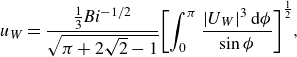 \begin{equation} {u_{W}} = \frac {\frac {1}{3}\textit{Bi}^{-1/2}}{\sqrt {\pi +2\sqrt {2} - 1}} {\left [ \int _0^\pi \frac {|{U_{W}}|^3\; \textrm {d} \phi }{\sin \phi } \right ]}^{\frac {1}{2}}, \end{equation}
from boundary-layer theory (§ C.1.2; Supekar et al. (Reference Supekar, Hewitt and Balmforth2020)). This criterion is consistent with a minimisation of the net dissipation rate (§ 3.3) because, hidden beyond the leading-order term in (5.5), lies a contribution of ${u_{W}} |{F_{X}}|$
from translation.
${u_{W}} |{F_{X}}|$
from translation.
Note that the force $F_{X}$
must vanish for a self-propelled squirmer. As indicated in figure 15(f), this condition selects the particular locomotion speed
$F_{X}$
must vanish for a self-propelled squirmer. As indicated in figure 15(f), this condition selects the particular locomotion speed ${u_{W}} \approx 1.54\textit{Bi}^{-1/2}$
, shown by the filled star. The analytical prediction from boundary-layer analysis
${u_{W}} \approx 1.54\textit{Bi}^{-1/2}$
, shown by the filled star. The analytical prediction from boundary-layer analysis
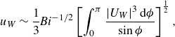 \begin{equation} {u_{W}} \sim \frac {1}{3} \textit{Bi}^{-1/2} \left [ \int _0^\pi \frac {|{U_{W}}|^3\; \textrm {d} \phi }{\sin \phi } \right ]^{\frac 12}, \end{equation}
(§ C.1.2; Supekar et al. (Reference Supekar, Hewitt and Balmforth2020)) is slightly smaller, as seen in figure 15(f).
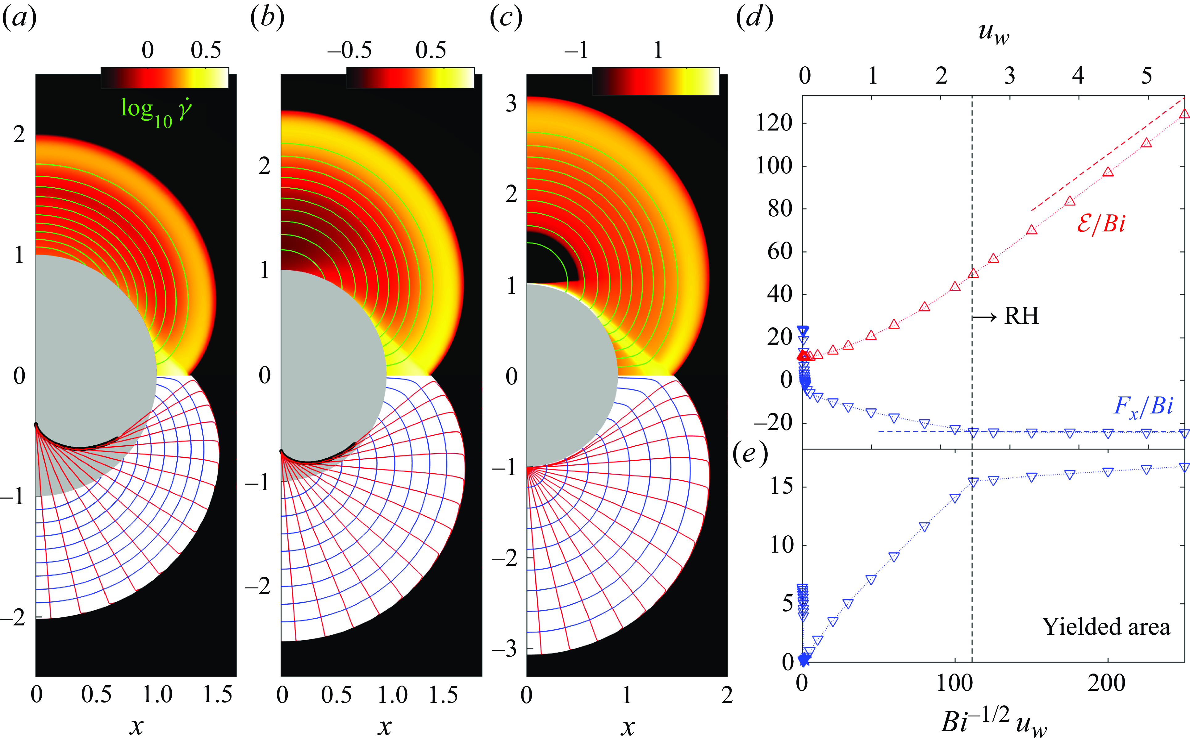
Figure 16. Model squirmers for higher translation speeds $u_{W}$
;
$u_{W}$
; $(n,\textit{Bi})=(1,2048)$
. On the left, strain-rate maps and sample streamlines are plotted for (a)
$(n,\textit{Bi})=(1,2048)$
. On the left, strain-rate maps and sample streamlines are plotted for (a) ${u_{W}}=45\textit{Bi}^{-1/2}\approx 1$
, (b)
${u_{W}}=45\textit{Bi}^{-1/2}\approx 1$
, (b) ${u_{W}}=80\textit{Bi}^{-1/2}\approx 1.77$
and (c)
${u_{W}}=80\textit{Bi}^{-1/2}\approx 1.77$
and (c) ${u_{W}}=250\textit{Bi}^{- 1/2}\approx 5.52$
. The lower half of the plots show slipline fields, constructed using the argument described in the main text. The thicker (red) lines in (a,b) reconstruct the curve inside the disk that appears to generate the involutes. A wider suite of computations with varying
${u_{W}}=250\textit{Bi}^{- 1/2}\approx 5.52$
. The lower half of the plots show slipline fields, constructed using the argument described in the main text. The thicker (red) lines in (a,b) reconstruct the curve inside the disk that appears to generate the involutes. A wider suite of computations with varying $u_{W}$
is presented on the right, plotting (d) the drag force
$u_{W}$
is presented on the right, plotting (d) the drag force $F_{X}$
and net dissipation rate
$F_{X}$
and net dissipation rate $\mathcal{E}$
, and (e) the yielded area. In (d), the (red and blue) dashed lines show (5.4) and
$\mathcal{E}$
, and (e) the yielded area. In (d), the (red and blue) dashed lines show (5.4) and $\mathcal{E}=|{F_{X}}|/u_{W}$
. The Randolph–Houlsby (RH) slipline pattern features to the right of the vertical line indicated.
$\mathcal{E}=|{F_{X}}|/u_{W}$
. The Randolph–Houlsby (RH) slipline pattern features to the right of the vertical line indicated.
Though not relevant to locomotion, one can consider much larger translation speeds of $O(1)$
, as illustrated in figure 16. Because the boundary-layer width grows with
$O(1)$
, as illustrated in figure 16. Because the boundary-layer width grows with $u_{W}$
, the flow delocalises again in this parameter range, forming a wider region of plastic deformation (panels (a,b)). Eventually, once this region extends sufficiently far from the disk, the pattern transforms into another with the Randolph & Houlsby form (panel (c)). The drag is then approximately given by (5.4), with a dissipation rate of
$u_{W}$
, the flow delocalises again in this parameter range, forming a wider region of plastic deformation (panels (a,b)). Eventually, once this region extends sufficiently far from the disk, the pattern transforms into another with the Randolph & Houlsby form (panel (c)). The drag is then approximately given by (5.4), with a dissipation rate of $\mathcal{E}\approx {u_{W}} {F_{X}}$
for large
$\mathcal{E}\approx {u_{W}} {F_{X}}$
for large $u_{W}$
.
$u_{W}$
.
The nearly plastic solution for ${u_{W}}\lesssim 2.45$
has an interesting structure, as highlighted by the slipline patterns shown in the lower halves of figure 16(a,b). Here, rather than attempt to reconstruct the slipline using the stress field (as in figure 10), we make use of the observation that there are no plugs within the yielded region and the
${u_{W}}\lesssim 2.45$
has an interesting structure, as highlighted by the slipline patterns shown in the lower halves of figure 16(a,b). Here, rather than attempt to reconstruct the slipline using the stress field (as in figure 10), we make use of the observation that there are no plugs within the yielded region and the $y$
-axis must correspond to a slipline as it is a line of symmetry. Hencky’s rules then imply all the sliplines of the same family as the
$y$
-axis must correspond to a slipline as it is a line of symmetry. Hencky’s rules then imply all the sliplines of the same family as the $y$
-axis are straight, and Geiringer’s equations demand that the other family correspond to streamlines. We therefore reconstruct the sliplines by finding contours of constant velocity direction and streamlines. This leads to the patterns shown in figure 16(a,b,c), with the latter largely reproducing the Randolph & Houlsby slipline field.
$y$
-axis are straight, and Geiringer’s equations demand that the other family correspond to streamlines. We therefore reconstruct the sliplines by finding contours of constant velocity direction and streamlines. This leads to the patterns shown in figure 16(a,b,c), with the latter largely reproducing the Randolph & Houlsby slipline field.
Note that the reconstruction fails once the sliplines cross a shear layer, which happens near the front and back of the disk, where the slipline pattern from the $y$
-axis meets the local checkerboards there. For
$y$
-axis meets the local checkerboards there. For ${u_{W}}\lesssim 2.45$
, the slipline field is composed of involutes generated by a curve lying inside the disk (see figure 16
a,b). Importantly, there is no boundary layer along the surface of the disk that dictates the slipline angle there (unlike for the Randolph–Houlsby patterns). The geometry of the curve from which the involutes are built must therefore be controlled by the strain-rates at the disk’s surface.
${u_{W}}\lesssim 2.45$
, the slipline field is composed of involutes generated by a curve lying inside the disk (see figure 16
a,b). Importantly, there is no boundary layer along the surface of the disk that dictates the slipline angle there (unlike for the Randolph–Houlsby patterns). The geometry of the curve from which the involutes are built must therefore be controlled by the strain-rates at the disk’s surface.
Finally, figure 17 presents solutions for a squirmer with a different surface velocity distribution. In this case, the angular surface velocity is more step-like, with $U_{W}(\phi )=\tanh (5\sin \phi )$
. Unlike in previous examples, the nearly plastic solution shown in figure 17(a) with
$U_{W}(\phi )=\tanh (5\sin \phi )$
. Unlike in previous examples, the nearly plastic solution shown in figure 17(a) with $u_{w}=0$
escapes the Randolph & Houlsby form, because of the appearance of a stress discontinuity (indicated by the green arrow; the yield surfaces are a little difficult to determine in this example owing to the presence of a wide region held very close to the yield stress). The discontinuity also appears to persist for the solution with much lower
$u_{w}=0$
escapes the Randolph & Houlsby form, because of the appearance of a stress discontinuity (indicated by the green arrow; the yield surfaces are a little difficult to determine in this example owing to the presence of a wide region held very close to the yield stress). The discontinuity also appears to persist for the solution with much lower $\textit{Bi}$
shown in figure 17(b), breaking into two pieces that each track curved yield lines (black arrows). The nearly vertical one close to
$\textit{Bi}$
shown in figure 17(b), breaking into two pieces that each track curved yield lines (black arrows). The nearly vertical one close to $y=\phi =0$
manifests mainly in the component
$y=\phi =0$
manifests mainly in the component ${\tau _{_{RR}}}=-{\tau _{_{\Phi \Phi }}}$
, in accord with the jump conditions stated in § 3.4.1. Thus, this squirmer offers another example in which stress discontinuities appear, even at finite
${\tau _{_{RR}}}=-{\tau _{_{\Phi \Phi }}}$
, in accord with the jump conditions stated in § 3.4.1. Thus, this squirmer offers another example in which stress discontinuities appear, even at finite $\textit{Bi}$
.
$\textit{Bi}$
.
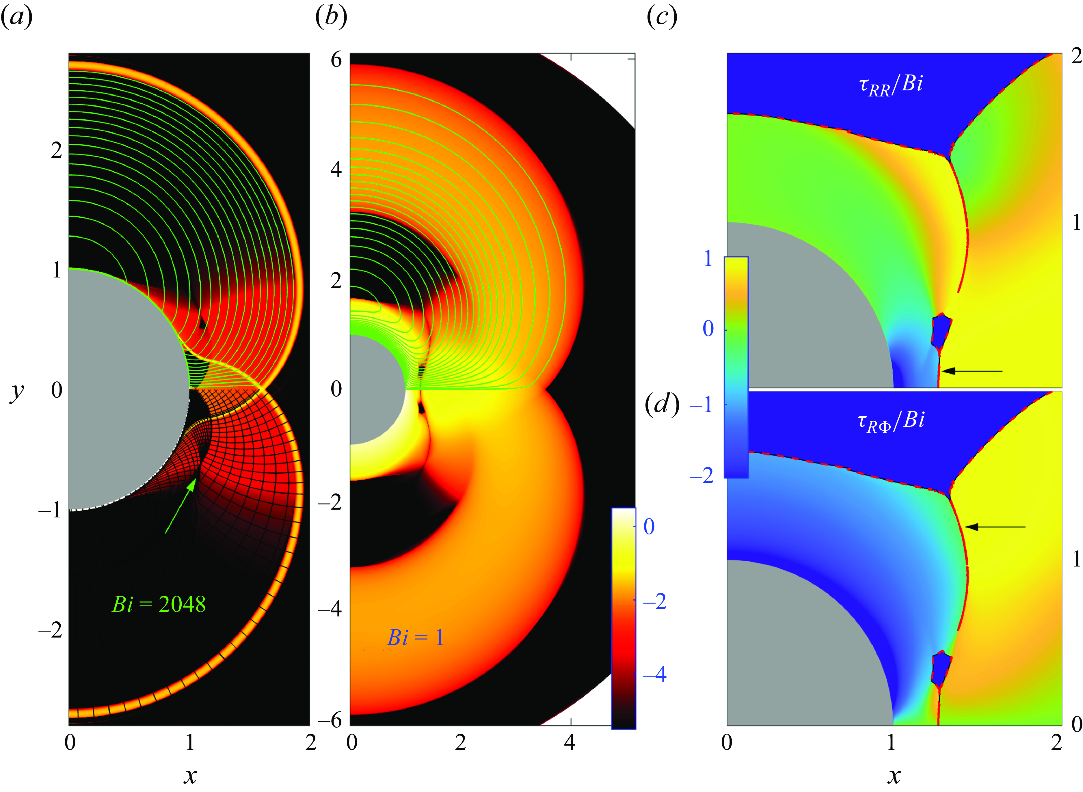
Figure 17. Sqirmer solutions for surface velocity, $u_{w}=0$
and
$u_{w}=0$
and $U_{W}(\phi )=\tanh (5\sin \phi )$
, and (a)
$U_{W}(\phi )=\tanh (5\sin \phi )$
, and (a) $\textit{Bi}=2048$
and (b)
$\textit{Bi}=2048$
and (b) $\textit{Bi}=1$
. Shown are sample streamlines (green) superposed on density maps of
$\textit{Bi}=1$
. Shown are sample streamlines (green) superposed on density maps of $\log _{10}{\dot \gamma }$
; in (a), the diagnosed slipline field is indicated by the black lines in
$\log _{10}{\dot \gamma }$
; in (a), the diagnosed slipline field is indicated by the black lines in $y\lt 0$
. Scaled stress components for the solution with
$y\lt 0$
. Scaled stress components for the solution with $\textit{Bi}=1$
are shown in (c,d). The plugs (diagnosed by the contour
$\textit{Bi}=1$
are shown in (c,d). The plugs (diagnosed by the contour ${\dot \gamma }=10^{-4}$
) are shaded dark blue with dashed red borders (the yield surfaces). The arrows point to what appear to be stress discontinuities.
${\dot \gamma }=10^{-4}$
) are shaded dark blue with dashed red borders (the yield surfaces). The arrows point to what appear to be stress discontinuities.
5.5. Translation with axial motion
Moving beyond two-dimensional flow, the relatively simple geometry of the annular gap (figure 9) offers a convenient setting in which to explore the impact of adding flow in the third spatial dimension on the dynamics in the nearly plastic limit. In particular, we can consider three-dimensional flow fields $(u,v,w)$
that depend only on the planar coordinates
$(u,v,w)$
that depend only on the planar coordinates $(x,y)$
. This task was accomplished by Hewitt & Balmforth (Reference Hewitt and Balmforth2018) and Hewitt & Balmforth (Reference Hewitt and Balmforth2022), who considered the flow around a cylinder translating at different angles to its axis, taking the annular gap to be sufficiently wide that the outer boundary is cloaked by a plug (rendering the problem equivalent to that of an infinitely long cylinder in an infinite domain). Further results for this problem are presented in figure 18. When the angle of motion is not closely aligned with the cylinder axis, the in-plane flow field is similar to the Randolph–Houlsby pattern; the boundary layers, shear layers and extended regions of nearly plastic deformation all survive the addition of an order-one out-of-plane velocity component (at large Bingham number). The nearly plastic regions, however, no longer possess an embedded slipline structure. Nevertheless, the structure of the two-dimensional flow pattern broadly carries over to a genuinely three-dimensional flow.
$(x,y)$
. This task was accomplished by Hewitt & Balmforth (Reference Hewitt and Balmforth2018) and Hewitt & Balmforth (Reference Hewitt and Balmforth2022), who considered the flow around a cylinder translating at different angles to its axis, taking the annular gap to be sufficiently wide that the outer boundary is cloaked by a plug (rendering the problem equivalent to that of an infinitely long cylinder in an infinite domain). Further results for this problem are presented in figure 18. When the angle of motion is not closely aligned with the cylinder axis, the in-plane flow field is similar to the Randolph–Houlsby pattern; the boundary layers, shear layers and extended regions of nearly plastic deformation all survive the addition of an order-one out-of-plane velocity component (at large Bingham number). The nearly plastic regions, however, no longer possess an embedded slipline structure. Nevertheless, the structure of the two-dimensional flow pattern broadly carries over to a genuinely three-dimensional flow.
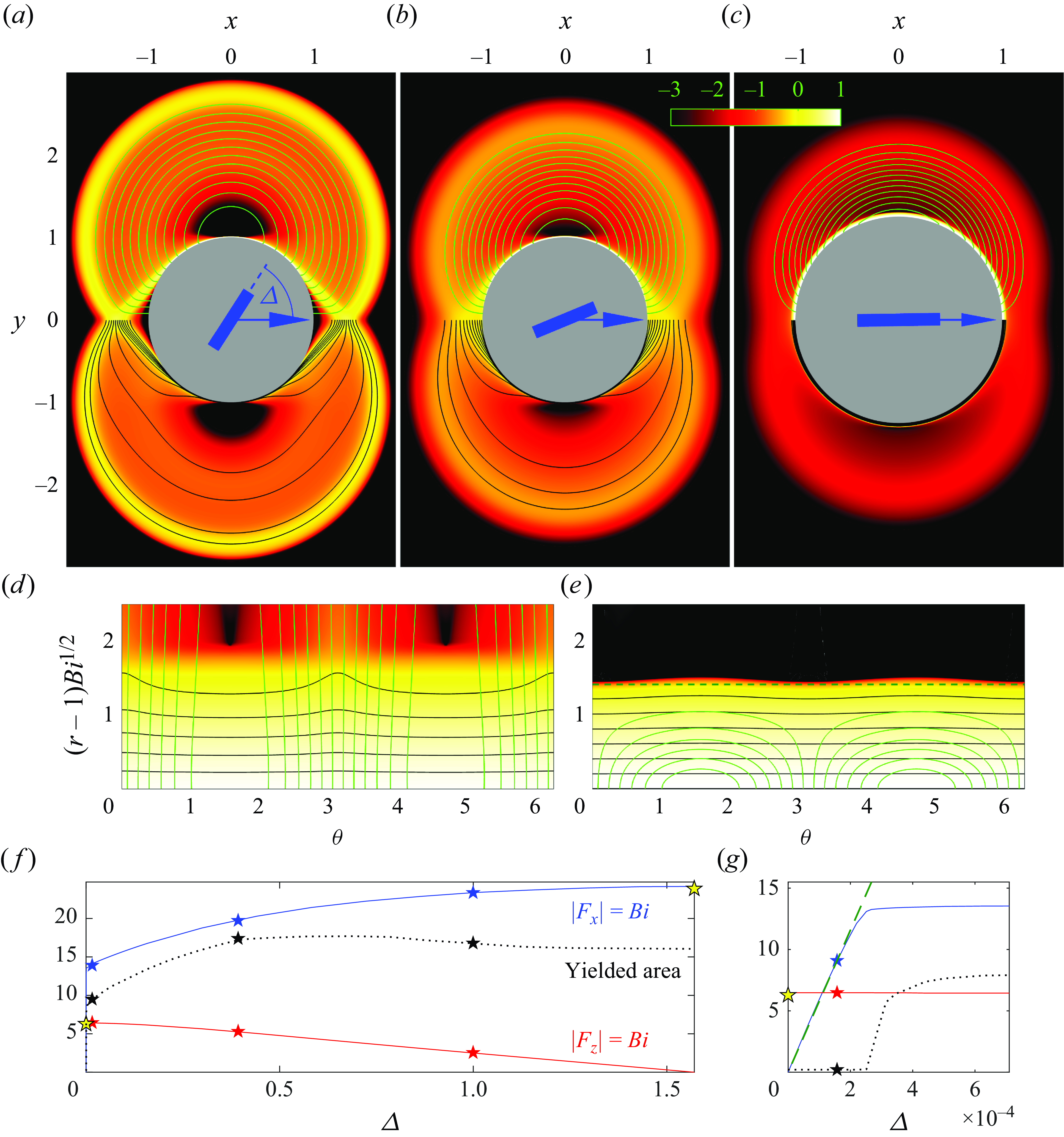
Figure 18. Flow around infinitely long cylinders translating with respect to their axes at angles $\unicode{x1D6E5}$
of (a)
$\unicode{x1D6E5}$
of (a) $ {7\pi }/{22}$
, (b)
$ {7\pi }/{22}$
, (b) $ \pi/ 8$
and (c)
$ \pi/ 8$
and (c) $ {\pi }/{200}$
. Shown are density plots of
$ {\pi }/{200}$
. Shown are density plots of $\log _{10}{\dot \gamma }$
with sample streamlines for the in-plane velocity field (green,
$\log _{10}{\dot \gamma }$
with sample streamlines for the in-plane velocity field (green, $y\gt 0$
) and contours of constant
$y\gt 0$
) and contours of constant $w$
(black,
$w$
(black, $y\lt 0$
).
$y\lt 0$
). $\textit{Bi}=2048$
. (d) A magnification of the boundary layer for the solution also shown in (c); panel (e) shows a similar plot for a fourth solution with localised boundary-layer flow at
$\textit{Bi}=2048$
. (d) A magnification of the boundary layer for the solution also shown in (c); panel (e) shows a similar plot for a fourth solution with localised boundary-layer flow at $\unicode{x1D6E5} =5\pi \times 10^{-5}$
. The force components,
$\unicode{x1D6E5} =5\pi \times 10^{-5}$
. The force components, $F_{X}$
and
$F_{X}$
and $F_{Z}$
(solid red and blue), and yielded area (dotted) are shown in (f) as functions of
$F_{Z}$
(solid red and blue), and yielded area (dotted) are shown in (f) as functions of $\unicode{x1D6E5}$
, for a wider set of computations. The filled stars show the angles for the solutions in (a,b,c,e), whereas the open (yellow) stars indicate the limits
$\unicode{x1D6E5}$
, for a wider set of computations. The filled stars show the angles for the solutions in (a,b,c,e), whereas the open (yellow) stars indicate the limits $({F_{X}},{F_{Z}})=(8\sqrt 2+4\pi, 0)\textit{Bi}$
and
$({F_{X}},{F_{Z}})=(8\sqrt 2+4\pi, 0)\textit{Bi}$
and $(0,2\pi )\textit{Bi}$
, expected for
$(0,2\pi )\textit{Bi}$
, expected for $\unicode{x1D6E5} =(1/2)\pi$
and
$\unicode{x1D6E5} =(1/2)\pi$
and $\unicode{x1D6E5} =0$
, respectively. Panel (g) replots the data for the small window of angles (of order
$\unicode{x1D6E5} =0$
, respectively. Panel (g) replots the data for the small window of angles (of order $\textit{Bi}^{-1}$
) over which the drag force reorientates. The dashed lines in (e) and (g) shows the predictions from boundary-layer analysis (Hewitt & Balmforth Reference Hewitt and Balmforth2022) of
$\textit{Bi}^{-1}$
) over which the drag force reorientates. The dashed lines in (e) and (g) shows the predictions from boundary-layer analysis (Hewitt & Balmforth Reference Hewitt and Balmforth2022) of ${F_{X}}\sim 9\pi \textit{Bi}^2\unicode{x1D6E5}$
and boundary-layer thickness (
${F_{X}}\sim 9\pi \textit{Bi}^2\unicode{x1D6E5}$
and boundary-layer thickness ( $\sqrt {2/\textit{Bi}}$
).
$\sqrt {2/\textit{Bi}}$
).
As the direction of motion becomes closer to axial, the flow pattern loses its similarity with the Randolph–Houlsby slipline field (see figure 18
b). More interestingly, when translation is almost completely aligned to the axial direction, fluid flow becomes primarily axial, and mostly confined to a narrow boundary layer around the cylinder (panel (c)). However, sideways motion still persists, generating a significant transverse force $F_{X}$
. Indeed, it is only when the direction of motion reaches a relatively narrow window of angles close to the axial direction (with a width of
$F_{X}$
. Indeed, it is only when the direction of motion reaches a relatively narrow window of angles close to the axial direction (with a width of $O(\textit{Bi}^{-2/(n+1)})$
) that the sideways force abruptly drops from
$O(\textit{Bi}^{-2/(n+1)})$
) that the sideways force abruptly drops from $O(\textit{Bi})$
values to zero (see figure 18
f,g). Hewitt & Balmforth (2018, 2022) focused on the impacts of this feature in swimming problems in which relatively long waves along a cylindrical worm or tail drive locomotion through a viscoplastic fluid. In particular, it was shown that because of the abrupt reorientation of the force, locomotion took the form of ‘burrowing’, with each cylindrical segment of the worm or tail moving almost axially (Hewitt Reference Hewitt2024).
$O(\textit{Bi})$
values to zero (see figure 18
f,g). Hewitt & Balmforth (2018, 2022) focused on the impacts of this feature in swimming problems in which relatively long waves along a cylindrical worm or tail drive locomotion through a viscoplastic fluid. In particular, it was shown that because of the abrupt reorientation of the force, locomotion took the form of ‘burrowing’, with each cylindrical segment of the worm or tail moving almost axially (Hewitt Reference Hewitt2024).
The sharp switch in the drag force arises because, in the perfectly plastic problem, axial motion can be accounted for purely by slip over the cylinder surface (which broadens into a viscoplastic boundary layer for finite $\textit{Bi}$
). But sideways translation, no matter how small, cannot. Thus, an arbitrarily small, but finite sideways translation must always create a region of perfectly plastic deformation away from the cylinder, generating a finite sideways drag. In the viscoplastic problem, this sideways drag can be switched off when the boundary layer against the cylinder consumes all motion, leading to the
$\textit{Bi}$
). But sideways translation, no matter how small, cannot. Thus, an arbitrarily small, but finite sideways translation must always create a region of perfectly plastic deformation away from the cylinder, generating a finite sideways drag. In the viscoplastic problem, this sideways drag can be switched off when the boundary layer against the cylinder consumes all motion, leading to the $O(\textit{Bi}^{-2/(n+1)})$
window of angles (a true boundary-layered solution from within this window is shown in figure 18
e). The switch from a localised boundary layer to extended sideways flow takes the form of a first-order transition in flow pattern in which part of the plug surrounding the cylinder breaks. The transition is visible in figure 18(g) as the kink in
$O(\textit{Bi}^{-2/(n+1)})$
window of angles (a true boundary-layered solution from within this window is shown in figure 18
e). The switch from a localised boundary layer to extended sideways flow takes the form of a first-order transition in flow pattern in which part of the plug surrounding the cylinder breaks. The transition is visible in figure 18(g) as the kink in $F_{X}$
and sharp rise in yielded area near
$F_{X}$
and sharp rise in yielded area near $\unicode{x1D6E5} =2.5\times 10^{-4}$
.
$\unicode{x1D6E5} =2.5\times 10^{-4}$
.
The perfectly plastic solution that emerges in the limit $\textit{Bi}\to \infty$
for translation angles
$\textit{Bi}\to \infty$
for translation angles $1\gg \unicode{x1D6E5} \gg O(\textit{Bi}^{-2/(n+1)})$
is similar to that for the translation of a two-dimensional disk with a free-slip condition on its surface (Martin & Randolph Reference Martin and Randolph2006; Supekar et al. Reference Supekar, Hewitt and Balmforth2020). This arises because most of the axial motion is confined to the viscous boundary layer; the in-plane velocities are much smaller, and not so confined. Viscoplastic boundary layer theory, on the other hand, demands that the stress components,
$1\gg \unicode{x1D6E5} \gg O(\textit{Bi}^{-2/(n+1)})$
is similar to that for the translation of a two-dimensional disk with a free-slip condition on its surface (Martin & Randolph Reference Martin and Randolph2006; Supekar et al. Reference Supekar, Hewitt and Balmforth2020). This arises because most of the axial motion is confined to the viscous boundary layer; the in-plane velocities are much smaller, and not so confined. Viscoplastic boundary layer theory, on the other hand, demands that the stress components, $\tau _{_{R\Phi }}$
and
$\tau _{_{R\Phi }}$
and $\tau _{_{RZ}}$
, dominate close to the cylinder. But this further implies that
$\tau _{_{RZ}}$
, dominate close to the cylinder. But this further implies that $\tau _{_{RZ}}\gg {\tau _{_{R\Phi }}}$
since
$\tau _{_{RZ}}\gg {\tau _{_{R\Phi }}}$
since $w\gg (u,v)$
. The boundary layer therefore enforces a stress-free condition on the plastic flow further from the cylinder. Nevertheless, the axial velocity does not vanish outside the boundary, and merely becomes as small as
$w\gg (u,v)$
. The boundary layer therefore enforces a stress-free condition on the plastic flow further from the cylinder. Nevertheless, the axial velocity does not vanish outside the boundary, and merely becomes as small as $u$
and
$u$
and $v$
. The problem does not therefore correspond precisely to flow around a two-dimensional, stress-free disk, although the flow pattern looks similar (see Supekar et al. (Reference Supekar, Hewitt and Balmforth2020)).
$v$
. The problem does not therefore correspond precisely to flow around a two-dimensional, stress-free disk, although the flow pattern looks similar (see Supekar et al. (Reference Supekar, Hewitt and Balmforth2020)).
6. Viscoplastic gravity currents
The final problem, sketched in figure 19, considers the viscoplastic analogue of a canonical problem in viscous fluid mechanics: a dambreak initiating a gravity current. This problem has wide application in geophysical and industrial settings, piecing together the viscoplastic failure of an emplaced block, the resulting gravity-driven runout, and the final convergence to a plastically arrested state. Figure 19 illustrates the configuration for the symmetrical version of this problem, in which a block collapses to both left and right, and shows the initial state at the moment of failure. The height of the block $\mathcal{H}$
can be taken as the length scale
$\mathcal{H}$
can be taken as the length scale $\mathcal{L}$
; the scaled half-width
$\mathcal{L}$
; the scaled half-width $\ell$
provides one of the parameters of the problem.
$\ell$
provides one of the parameters of the problem.

Figure 19. Sketch of the collapse of a block of yield-stress fluid with finite density immersed in a miscible viscous fluid with negligible density. The computational domain contains exactly half of the block. The characteristic length scale is set by the height of the block $\mathcal{H}$
, and a characteristic speed
$\mathcal{H}$
, and a characteristic speed $\mathcal{U}$
is then taken to be
$\mathcal{U}$
is then taken to be $\rho g \mathcal{H}^2/{\mu }$
.
$\rho g \mathcal{H}^2/{\mu }$
.
The other main parameter (setting aside $n$
) is a measure of the yield stress. In this case, we cannot immediately define the usual Bingham number because there is no specified velocity scale
$n$
) is a measure of the yield stress. In this case, we cannot immediately define the usual Bingham number because there is no specified velocity scale $\mathcal{U}$
. Instead, the distance over which the yield stress competes against gravity can be gauged by the length scale
$\mathcal{U}$
. Instead, the distance over which the yield stress competes against gravity can be gauged by the length scale ${\tau _{_{_P}}}/(\rho g)$
, leading us to define the parameter
${\tau _{_{_P}}}/(\rho g)$
, leading us to define the parameter
 \begin{equation} \textit{Bi} = \frac {{\tau _{_{_P}}}}{\rho g \mathcal{H}} . \end{equation}
A balance between the gravitational stress scale $\rho g \mathcal{H}$
and the viscous stress
$\rho g \mathcal{H}$
and the viscous stress $K(\mathcal{U}/\mathcal{H})^n$
, then implies a convenient velocity scale
$K(\mathcal{U}/\mathcal{H})^n$
, then implies a convenient velocity scale
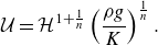 \begin{equation} \mathcal{U} = \mathcal{H}^{1+\frac 1n} \left ( \frac {\rho g}{K} \right )^{\frac 1n} . \end{equation}
With this choice, we could replace (6.1) with the original definition of the Bingham number in (2.3), and we continue to informally refer to $\textit{Bi}$
in that fashion with this in mind. However, as defined in (6.1),
$\textit{Bi}$
in that fashion with this in mind. However, as defined in (6.1), $\textit{Bi}$
is more properly interpreted as the ratio of the yield stress to the externally imposed, gravitational stress scale (which is often referred to as the Oldroyd number).
$\textit{Bi}$
is more properly interpreted as the ratio of the yield stress to the externally imposed, gravitational stress scale (which is often referred to as the Oldroyd number).
6.1. Failure
Failure problems like the initial collapse of the block in figure 19 are commonplace in geotechnical engineering, in addressing the stability of slopes, embankments and other structures (Terzaghi Reference Terzaghi1943). For cohesive soil, the problem is traditionally dealt with within the framework of ideal plasticity theory, which corresponds to the plastic limit for failure of a block of yield-stress fluid. The problem is also more commonly couched in terms of the limit analysis of plasticity (Prager & Hodge Reference Prager and Hodge1951), wherein one exploits the corresponding extremum principles to § 3.3 to provide bounds on the critical value of $\textit{Bi}$
at which failure occurs.
$\textit{Bi}$
at which failure occurs.
For a rectangular block, the critical value for failure, $\textit{Bi}_{crit}$
, depends on the aspect ratio
$\textit{Bi}_{crit}$
, depends on the aspect ratio $\ell$
(Liu et al. Reference Liu, Balmforth, Hormozi and Hewitt2016), as summarised in figure 20(a). In addition, at
$\ell$
(Liu et al. Reference Liu, Balmforth, Hormozi and Hewitt2016), as summarised in figure 20(a). In addition, at $\textit{Bi}=\textit{Bi}_{crit}$
deformation adopts a specific spatial pattern, or ‘failure mode’. Such patterns correspond to the dynamical modes for incipient collapse in elastic systems, or the neutral modes at the onset of linear instability in a viscous flow, with the critical value
$\textit{Bi}=\textit{Bi}_{crit}$
deformation adopts a specific spatial pattern, or ‘failure mode’. Such patterns correspond to the dynamical modes for incipient collapse in elastic systems, or the neutral modes at the onset of linear instability in a viscous flow, with the critical value $\textit{Bi}_{crit}(\ell )$
playing the role of the stability threshold. However, the yield stress ensures that viscoplastic failure is equivalent to a nonlinear eigenproblem (with an indeterminate equilibrium stress), unlike a conventional linear stability analysis. Demanding symmetry along
$\textit{Bi}_{crit}(\ell )$
playing the role of the stability threshold. However, the yield stress ensures that viscoplastic failure is equivalent to a nonlinear eigenproblem (with an indeterminate equilibrium stress), unlike a conventional linear stability analysis. Demanding symmetry along $x=0$
also rules out failure modes that correspond to sideways buckling, divorcing the current formulation from the classical problem of Euler’s elastic column.
$x=0$
also rules out failure modes that correspond to sideways buckling, divorcing the current formulation from the classical problem of Euler’s elastic column.
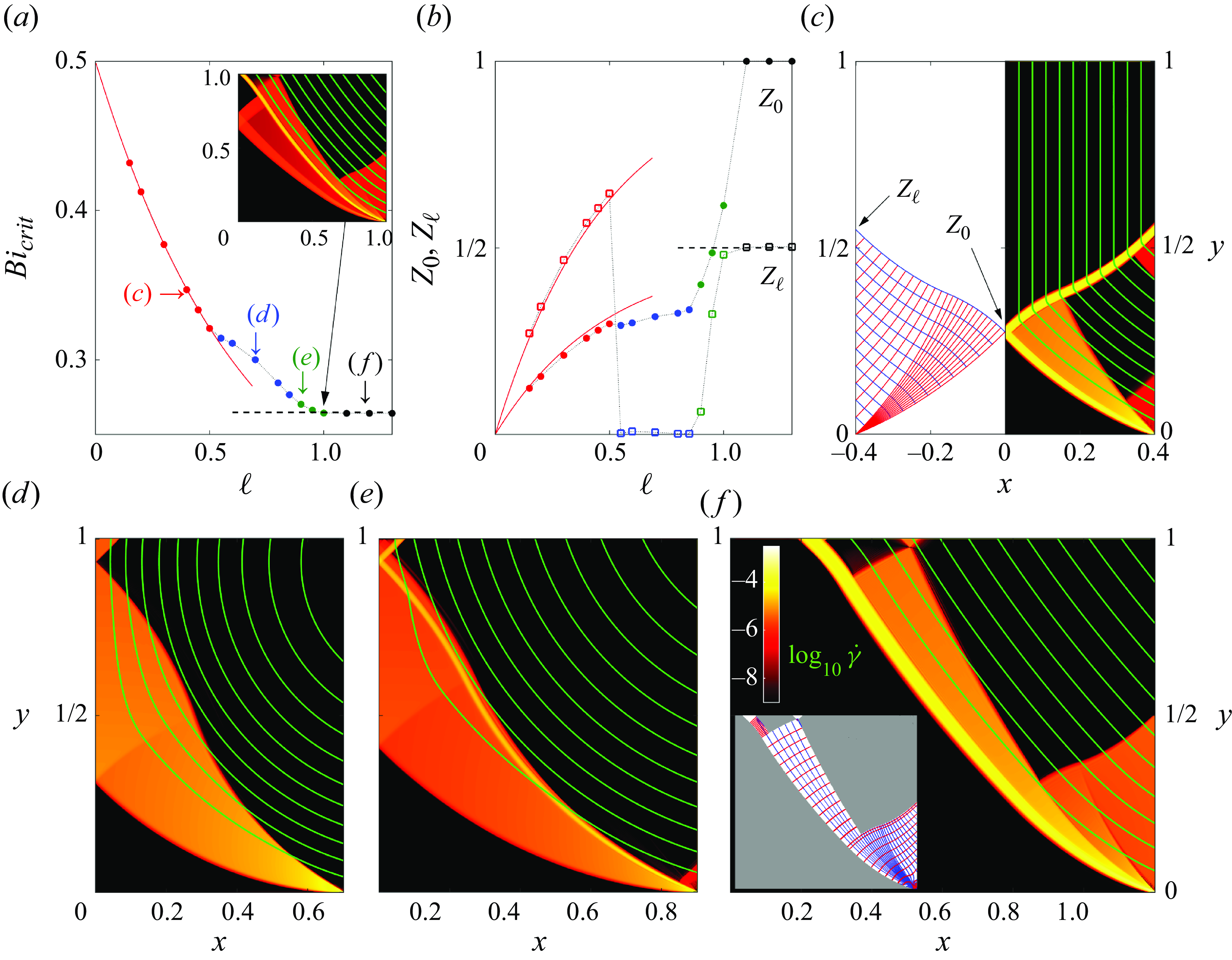
Figure 20. Failure modes for the problem sketched in figure 19. (a) The critical Bingham number $\textit{Bi}_{crit}$
above which there is no motion as a function of the aspect ratio
$\textit{Bi}_{crit}$
above which there is no motion as a function of the aspect ratio $\ell = \mathcal{L}/\mathcal{H}$
, and (b) the heights,
$\ell = \mathcal{L}/\mathcal{H}$
, and (b) the heights, $Z_0$
(filled circles) and
$Z_0$
(filled circles) and $Z_\ell$
(open squares), at which failure occurs along
$Z_\ell$
(open squares), at which failure occurs along $x=0$
and
$x=0$
and $x=\ell$
, respectively. Four distinct modes are identified in (a,b) and plotted with different colours; samples of each are illustrated in the remaining panels (e–f), which present density plots of
$x=\ell$
, respectively. Four distinct modes are identified in (a,b) and plotted with different colours; samples of each are illustrated in the remaining panels (e–f), which present density plots of $\log _{10}(\dot \gamma )$
along with selected streamlines. The solution at
$\log _{10}(\dot \gamma )$
along with selected streamlines. The solution at $\ell =1$
, shown further in the inset to panel (a), appears to have mixed character. In (c), a corresponding slipline pattern is also shown (in
$\ell =1$
, shown further in the inset to panel (a), appears to have mixed character. In (c), a corresponding slipline pattern is also shown (in $x\lt 0$
); the predictions of slipline theory are shown by (red) solid lines in (a,b). The dashed lines in (a,b) indicates the aspect-ratio-independent theoretical limit for
$x\lt 0$
); the predictions of slipline theory are shown by (red) solid lines in (a,b). The dashed lines in (a,b) indicates the aspect-ratio-independent theoretical limit for $\ell \gt 1$
(Lyamin & Sloan Reference Lyamin and Sloan2002a
,Reference Lyamin and Sloan
b
; Martin Reference Martin2011). The inset to (f) shows a reconstruction of the slipline field. The failure modes here are identified by computing solutions at sequentially larger
$\ell \gt 1$
(Lyamin & Sloan Reference Lyamin and Sloan2002a
,Reference Lyamin and Sloan
b
; Martin Reference Martin2011). The inset to (f) shows a reconstruction of the slipline field. The failure modes here are identified by computing solutions at sequentially larger $\textit{Bi}$
until the maximum strain rate over the block,
$\textit{Bi}$
until the maximum strain rate over the block, ${\dot \gamma }_{max}$
, falls below
${\dot \gamma }_{max}$
, falls below $2\times 10^{-3}$
; the critical Bingham number is then determined by extrapolating
$2\times 10^{-3}$
; the critical Bingham number is then determined by extrapolating ${\dot \gamma }_{max}$
to zero.
${\dot \gamma }_{max}$
to zero.
For relatively slender blocks, the column of material fails primarily at its base, below a vertically falling plug. The distinctive flow pattern, or the failure mode, that results is illustrated in figure 20(c), and can be built by slipline theory (Chamberlain et al. Reference Chamberlain, Sader, Landman and White2001). The slipline pattern, also shown in the figure, contains a checkerboard stemming from the free surface at the side, together with a fan emanating from the lower outer corner. The sliplines in both are no longer straight, but curve because of gravity and the impact of hydrostatic pressure on the slipline invariants (see Appendix B.4). Note that a section of the expected plastic region appears to plug up in the computation, a feature permitted by the shear layer along its top border. This leads to a serendipitous plug at the side that rotates out of position.
The slipline solution illustrated in figure 20(c) provides a prediction for $\textit{Bi}_{crit}(\ell )$
that is added to figure 20(a). Other properties of the failure mode can also be established, such as the heights,
$\textit{Bi}_{crit}(\ell )$
that is added to figure 20(a). Other properties of the failure mode can also be established, such as the heights, $Z_0$
and
$Z_0$
and $Z_\ell$
, up to which failure occurs at
$Z_\ell$
, up to which failure occurs at $x=0$
and
$x=0$
and $x=\ell$
, respectively (cf. figure 20
c). These alternative measures offer clearer diagnostics of the transitions in flow patterns (or failure mode) that take place as the aspect ratio is varied; see figure 20(b). The first transition arises for
$x=\ell$
, respectively (cf. figure 20
c). These alternative measures offer clearer diagnostics of the transitions in flow patterns (or failure mode) that take place as the aspect ratio is varied; see figure 20(b). The first transition arises for $\ell \approx 0.5$
and is first order, involving the breakage of the upper plug along the symmetry line. The breakage eliminates purely vertical collapse (and the slipline field of panel (c)), and instead permits the upper corners of the initial block to rotate out sideways. Widespread plastic deformation takes places underneath the rigid rotation.
$\ell \approx 0.5$
and is first order, involving the breakage of the upper plug along the symmetry line. The breakage eliminates purely vertical collapse (and the slipline field of panel (c)), and instead permits the upper corners of the initial block to rotate out sideways. Widespread plastic deformation takes places underneath the rigid rotation.
The failure mode changes again when the aspect ratio $\ell$
reaches values closer to unity, with a prominent shear layer emerging that pierces the block close to its core. Figure 20 identifies what appear to be four distinct failure modes altogether. In panels (a,b), the four modes are plotted with different colours, and examples of each mode are shown in (c,d,e,f). In these failure computations (which proceed in an iterative manner in order to determine
$\ell$
reaches values closer to unity, with a prominent shear layer emerging that pierces the block close to its core. Figure 20 identifies what appear to be four distinct failure modes altogether. In panels (a,b), the four modes are plotted with different colours, and examples of each mode are shown in (c,d,e,f). In these failure computations (which proceed in an iterative manner in order to determine $\textit{Bi}_{crit}$
), the modes and the transitions between them are less straightforward to characterise because strain rates are necessarily small, which can obscure the geometry of the yield surfaces, plugs and plastic regions.
$\textit{Bi}_{crit}$
), the modes and the transitions between them are less straightforward to characterise because strain rates are necessarily small, which can obscure the geometry of the yield surfaces, plugs and plastic regions.
Once $\ell$
exceeds unity, collapse only arises in the vicinity of the vertical face (figure 20
f); the central core of the block never fails, and the critical value becomes independent of aspect ratio. The solution then corresponds to the failure mode of an infinitely wide block, bounds for which have been provided by Lyamin & Sloan (Reference Lyamin and Sloan2002a
,Reference Lyamin and Sloan
b
). This failure mode has
$\ell$
exceeds unity, collapse only arises in the vicinity of the vertical face (figure 20
f); the central core of the block never fails, and the critical value becomes independent of aspect ratio. The solution then corresponds to the failure mode of an infinitely wide block, bounds for which have been provided by Lyamin & Sloan (Reference Lyamin and Sloan2002a
,Reference Lyamin and Sloan
b
). This failure mode has $\textit{Bi}_{crit}\approx 0.2648$
,
$\textit{Bi}_{crit}\approx 0.2648$
, $Z_0=1$
and
$Z_0=1$
and $Z_\ell \approx (1/2)$
(as seen in figure 20
a,b), and possesses a slipline solution that has been constructed by Martin (Reference Martin2011). This slipline field is rather intricate, however, and Martin’s strategy to build it is more like our slipline reconstruction from the numerical viscoplastic flow computation (cf. the inset in figure 20
f) than an explicit construction using the slipline equations, as in Appendix B. In fact, beyond the relatively narrow limit, the modes of failure and their corresponding slipline patterns are fairly complicated; for no aspect ratio do they take the form of simple arcs of failure between rigid blocks (as is often assumed in the geotechnical engineering literature in order to establish simple bounds; e.g. Terzaghi (Reference Terzaghi1943); Chamberlain et al. (Reference Chamberlain, Horrobin, Landman and Sader2004)). Nevertheless, the failure modes again form the patchwork of plugs, plastic regions and boundary layers that we now expect in the plastic limit.
$Z_\ell \approx (1/2)$
(as seen in figure 20
a,b), and possesses a slipline solution that has been constructed by Martin (Reference Martin2011). This slipline field is rather intricate, however, and Martin’s strategy to build it is more like our slipline reconstruction from the numerical viscoplastic flow computation (cf. the inset in figure 20
f) than an explicit construction using the slipline equations, as in Appendix B. In fact, beyond the relatively narrow limit, the modes of failure and their corresponding slipline patterns are fairly complicated; for no aspect ratio do they take the form of simple arcs of failure between rigid blocks (as is often assumed in the geotechnical engineering literature in order to establish simple bounds; e.g. Terzaghi (Reference Terzaghi1943); Chamberlain et al. (Reference Chamberlain, Horrobin, Landman and Sader2004)). Nevertheless, the failure modes again form the patchwork of plugs, plastic regions and boundary layers that we now expect in the plastic limit.
6.2. Runout; thin-film spreading
After failure, the block collapses into a free-surface gravity current that runs out to lower the gravitational stresses towards the yield stress everywhere. The time-dependent dynamics of the spreading gravity current can be interrogated by numerical simulation (see Liu et al. (Reference Liu, Balmforth, Hormozi and Hewitt2016) and references therein; Valette et al. (Reference Valette, Pereira, Riber, Sardo, Larcher and Hachem2021)), although computations can be time consuming and tricky. An alternative is to assume that flows are relatively shallow ( $\ell \ll 1$
) and exploit lubrication theory, as has been done for viscous gravity currents (e.g. Huppert Reference Huppert1982). Balmforth et al. (Reference Balmforth, Craster, Rust and Sassi2006) and Appendix C.2.2 review details of the viscoplastic version of this analysis, which furnishes an evolution equation for the local depth of the fluid layer
$\ell \ll 1$
) and exploit lubrication theory, as has been done for viscous gravity currents (e.g. Huppert Reference Huppert1982). Balmforth et al. (Reference Balmforth, Craster, Rust and Sassi2006) and Appendix C.2.2 review details of the viscoplastic version of this analysis, which furnishes an evolution equation for the local depth of the fluid layer $h(x,t)$
. Related situations in which the analysis has been exploited include bearings and blade coating (Hewitt & Balmforth Reference Hewitt and Balmforth2012; Lister & Hinton Reference Lister and Hinton2022), the flow of lava and mud (Blake Reference Blake1990; Hinton & Hogg Reference Hinton and Hogg2022; Hinton, Hewitt & Hogg Reference Hinton, Hewitt and Hogg2023), the growth of mountain ranges (Ribinskas et al. Reference Ribinskas, Ball, Penney and Neufeld2024; Taylor-West & Hogg Reference Taylor-West and Hogg2024), the viscoplastic linings of lung airways (Shemilt et al. Reference Shemilt, Horsley, Jensen, Thompson and Whitfield2022, Reference Shemilt, Horsley, Jensen, Thompson and Whitfield2023) and other problems involving surface tension (Ross, Wilson & Duffy Reference Ross, Wilson and Duffy2001; Jalaal & Balmforth Reference Jalaal and Balmforth2016; Jalaal, Stoeber & Balmforth Reference Jalaal, Stoeber and Balmforth2021; Ball & Balmforth Reference Ball and Balmforth2024).
$h(x,t)$
. Related situations in which the analysis has been exploited include bearings and blade coating (Hewitt & Balmforth Reference Hewitt and Balmforth2012; Lister & Hinton Reference Lister and Hinton2022), the flow of lava and mud (Blake Reference Blake1990; Hinton & Hogg Reference Hinton and Hogg2022; Hinton, Hewitt & Hogg Reference Hinton, Hewitt and Hogg2023), the growth of mountain ranges (Ribinskas et al. Reference Ribinskas, Ball, Penney and Neufeld2024; Taylor-West & Hogg Reference Taylor-West and Hogg2024), the viscoplastic linings of lung airways (Shemilt et al. Reference Shemilt, Horsley, Jensen, Thompson and Whitfield2022, Reference Shemilt, Horsley, Jensen, Thompson and Whitfield2023) and other problems involving surface tension (Ross, Wilson & Duffy Reference Ross, Wilson and Duffy2001; Jalaal & Balmforth Reference Jalaal and Balmforth2016; Jalaal, Stoeber & Balmforth Reference Jalaal, Stoeber and Balmforth2021; Ball & Balmforth Reference Ball and Balmforth2024).
Figure 21. A shallow-layer solution to (C39) for the collapse of a block above a horizontal base plate for $\textit{Bi}=0.004$
and
$\textit{Bi}=0.004$
and $\ell =10$
. The initial shape is given by
$\ell =10$
. The initial shape is given by $h(x,0)=h_\infty +1+\tanh [100(x-(1/2)\ell )]$
, where
$h(x,0)=h_\infty +1+\tanh [100(x-(1/2)\ell )]$
, where $h_\infty =10^{-3}$
denotes a pre-wetted film coating the entire base plate (added to ease numerical computations, along with the regularisation parameter,
$h_\infty =10^{-3}$
denotes a pre-wetted film coating the entire base plate (added to ease numerical computations, along with the regularisation parameter, $Y_\infty =10^{-6}$
, introduced in the replacement
$Y_\infty =10^{-6}$
, introduced in the replacement $Y=$
Max
$Y=$
Max $(Y_\infty, h-\textit{Bi}/|\partial h / \partial x|)$
in (C39)). The geometry of the slump is sketched in (a). Panel (b) shows snapshots of
$(Y_\infty, h-\textit{Bi}/|\partial h / \partial x|)$
in (C39)). The geometry of the slump is sketched in (a). Panel (b) shows snapshots of $h(x,t)$
and
$h(x,t)$
and $Y(x,t)$
; the final profile of
$Y(x,t)$
; the final profile of $h(x,t)$
(as given by (6.3)) is shown by the red dots. In (c), scaled snapshots of
$h(x,t)$
(as given by (6.3)) is shown by the red dots. In (c), scaled snapshots of $Y$
and
$Y$
and $u_p$
for
$u_p$
for $t\gt 0.1$
are plotted against
$t\gt 0.1$
are plotted against $\xi =x/X(t)$
(with
$\xi =x/X(t)$
(with $X(t)$
defined by
$X(t)$
defined by $h(X,t)=1.01h_\infty$
);
$h(X,t)=1.01h_\infty$
); $Y$
is scaled by its maximum value,
$Y$
is scaled by its maximum value, $u_p$
by twice the value taken where
$u_p$
by twice the value taken where $\xi =(2/3)$
. Panel (d) shows times series of
$\xi =(2/3)$
. Panel (d) shows times series of $h_m(t)=h(0,t)$
and
$h_m(t)=h(0,t)$
and $X(t)$
, with the dashed lines show the predictions from solving (C46).
$X(t)$
, with the dashed lines show the predictions from solving (C46).
Figure 21 presents a sample numerical solution to the thin-film evolution equation (C39), in which a block of fluid collapses and runs out over the underlying horizontal plane. Note that, because shear stresses vanish along the free surface (in the absence of surface tension), a superficial pseudo-plug must appear during runout, as sketched in figure 21(a). The relatively strongly sheared layer underneath the pseudo-plug has depth $Y(x,t)\equiv h-\textit{Bi}/|\partial h / \partial x|$
; as the fluid runs out, and surface slopes and stresses decline, this depth descends to
$Y(x,t)\equiv h-\textit{Bi}/|\partial h / \partial x|$
; as the fluid runs out, and surface slopes and stresses decline, this depth descends to $y=0$
. Importantly, runout becomes limited by the yield stress and fluid eventually reaches a slumped state with a sloped surface, unlike in the corresponding viscous problem (in the absence of surface tension).
$y=0$
. Importantly, runout becomes limited by the yield stress and fluid eventually reaches a slumped state with a sloped surface, unlike in the corresponding viscous problem (in the absence of surface tension).
As noted by Nye (Reference Nye1951) and others, the final state is given by $Y\to 0$
, or
$Y\to 0$
, or
 \begin{equation} h = \sqrt { 2\textit{Bi} (X-x)}, \end{equation}
where $x=X$
denotes the fluid edge (see Appendix C.2.2). In the example shown in figure 21, the entire block yields and flows on its path to the final state. When the initial block is sufficiently wide, or the yield stress large enough, however, part of the block remains intact, leaving a flat-topped final deposit (Balmforth et al. Reference Balmforth, Craster, Rust and Sassi2006). Here, we consider only fully collapsed states.
$x=X$
denotes the fluid edge (see Appendix C.2.2). In the example shown in figure 21, the entire block yields and flows on its path to the final state. When the initial block is sufficiently wide, or the yield stress large enough, however, part of the block remains intact, leaving a flat-topped final deposit (Balmforth et al. Reference Balmforth, Craster, Rust and Sassi2006). Here, we consider only fully collapsed states.
The convergence to the final state can be described analytically and follows a relatively long, algebraic dependence on time (see Matson & Hogg (Reference Matson and Hogg2007); Hogg & Matson (Reference Hogg and Matson2009); Appendix C.2.2). For a Bingham fluid the convergence takes the form $t^{-1}$
, as illustrated in figure 21(d). During this passage,
$t^{-1}$
, as illustrated in figure 21(d). During this passage, $\partial u_{p}/\partial x\gt 0$
, where
$\partial u_{p}/\partial x\gt 0$
, where $u_p$
is the speed of the pseudo-plug, indicating a state of horizontal expansion (cf. figure 21
c).
$u_p$
is the speed of the pseudo-plug, indicating a state of horizontal expansion (cf. figure 21
c).
Note that dambreaks from a step-like initial condition are problematic in lubrication theory because $|\partial h / \partial x|$
becomes arbitrarily large at the step, but should be asymptotically small for the theory to remain valid (which is partly why the step in the initial condition in figure 21 has been smoothed out slightly). Lubrication theory cannot therefore address the initial failure of the block, as in § 6.1. Indeed, the theory predicts that the block always fails (the yield criterion being
$|\partial h / \partial x|$
becomes arbitrarily large at the step, but should be asymptotically small for the theory to remain valid (which is partly why the step in the initial condition in figure 21 has been smoothed out slightly). Lubrication theory cannot therefore address the initial failure of the block, as in § 6.1. Indeed, the theory predicts that the block always fails (the yield criterion being $Y=h-\textit{Bi}/|\partial h / \partial x|\gt 0$
, which is inevitably satisfied if
$Y=h-\textit{Bi}/|\partial h / \partial x|\gt 0$
, which is inevitably satisfied if $|\partial h / \partial x|\to \infty$
).
$|\partial h / \partial x|\to \infty$
).
6.3. Slumped states with finite slope
Armed with slipline theory, one can attempt to advance beyond the thin-film limit and build the final shape for slumps with finite slope. In this context, Nye provided an elegant construction for gravity-driven plastic flow with a free surface in the context of modelling the shape of the snout of a glacier. This construction applies equally to viscoplastic flow in the plastic limit.
Details of Nye’s construction are provided in Appendix B.4, which begins by artificially providing data along the outer arc of a circular fan, as illustrated in figure 22(a). The opening angle of the fan and its height $h_0$
act as two parameters. The surprising feature of Nye’s construct is that, as one proceeds to shallower depths, the slipline field converges to a special solution regardless of the precise details of the initial slipline (i.e. the fan angle and
$h_0$
act as two parameters. The surprising feature of Nye’s construct is that, as one proceeds to shallower depths, the slipline field converges to a special solution regardless of the precise details of the initial slipline (i.e. the fan angle and $h_0$
). Indeed, another choice for the initial slipline based on Prandtl’s cycloid (see Appendix B.4) leads to the slipline field shown in figure 22(b). This alternative construction converges more quickly to the special solution.
$h_0$
). Indeed, another choice for the initial slipline based on Prandtl’s cycloid (see Appendix B.4) leads to the slipline field shown in figure 22(b). This alternative construction converges more quickly to the special solution.
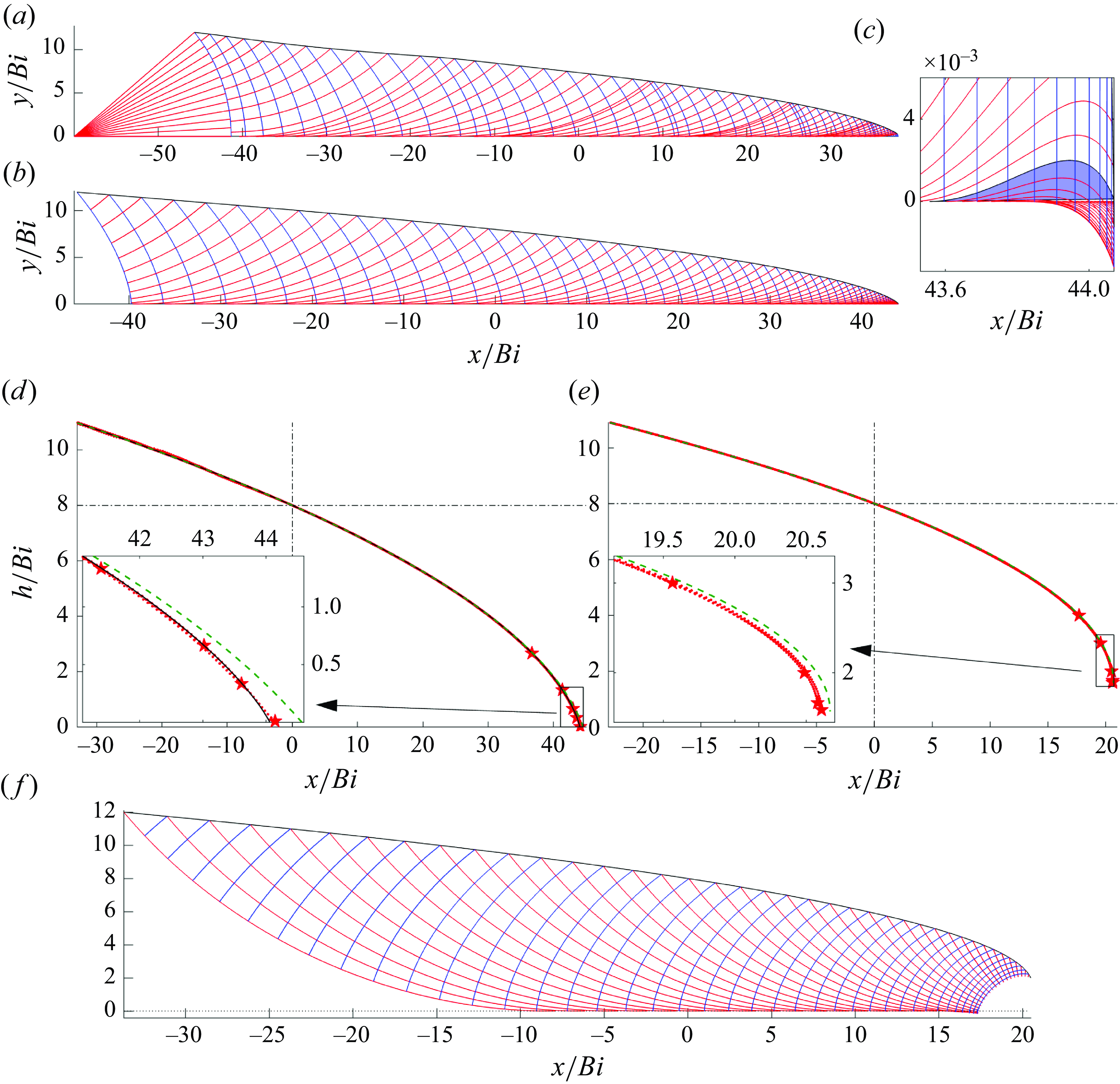
Figure 22. Surface profiles constructed for (a–d) horizontal extension and (e,f) horizontal compression. Nye’s original construction of the slipline field from part of a circular fan is shown in (a); the construction in (b) uses a modified Prandtl cycloid to launch the sliplines. In (c), a magnification near the nose is shown for the slipline field of (b); the shaded region indicates the plug introduced by Nye to avoid the sliplines unphysically turning downwards from $y=0$
. The constructions in (d,e) uses the minimisation scheme outlined in Appendix B.4 to build the slipline field using a section of the free surface for
$y=0$
. The constructions in (d,e) uses the minimisation scheme outlined in Appendix B.4 to build the slipline field using a section of the free surface for $h_1 \gt (h/Bi) \gt h_2$
with
$h_1 \gt (h/Bi) \gt h_2$
with $h_1=12$
and
$h_1=12$
and $h_2=2$
. The red dots show surface profiles constructed for the different values of
$h_2=2$
. The red dots show surface profiles constructed for the different values of $h_2$
marked by stars (
$h_2$
marked by stars ( $h_2=0.505\pi$
,
$h_2=0.505\pi$
, $(5/3)$
, 2, 3 and 4 in (c);
$(5/3)$
, 2, 3 and 4 in (c); $h_2=0.01$
,
$h_2=0.01$
, $(1/3)$
,
$(1/3)$
, $(2/3)$
,
$(2/3)$
, $(4/3)$
and
$(4/3)$
and $(8/3)$
in (e)). The dashed lines show the profile predicted by (higher-order) shallow-layer theory. The solid line in (d) shows the profile from (b). All the profiles are aligned at the surface height
$(8/3)$
in (e)). The dashed lines show the profile predicted by (higher-order) shallow-layer theory. The solid line in (d) shows the profile from (b). All the profiles are aligned at the surface height $h=8$
indicated by the dot-dashed lines. The overlaid plots in (d,e) show magnifications near the nose.
$h=8$
indicated by the dot-dashed lines. The overlaid plots in (d,e) show magnifications near the nose.
The profile of the special solution is displayed in figure 22(d). One awkward detail of this solution is that the steepening of the free surface near the fluid edge inevitably leads to the lowest $\alpha $
-line eventually curving downwards rather than upwards into the fluid (see Nye (Reference Nye1951) and Appendix B.4). Nye argued that this breakdown of the special solution could by cured by placing a plug below the distinguished
$\alpha $
-line eventually curving downwards rather than upwards into the fluid (see Nye (Reference Nye1951) and Appendix B.4). Nye argued that this breakdown of the special solution could by cured by placing a plug below the distinguished $\alpha $
-line that curves initially upwards from the base before descending and intersecting the fluid edge, as illustrated by the shaded region in figure 22(c).
$\alpha $
-line that curves initially upwards from the base before descending and intersecting the fluid edge, as illustrated by the shaded region in figure 22(c).
Unfortunately, Nye’s construction is not relevant to the dambreak problem shown in figure 21: his glacier snout is assumed to be in a state of horizontal compression. By contrast, as illustrated in figure 21(c), shallow viscoplastic dambreaks reach their the final state under horizontal expansion, a result that carries over to finite depths (Liu et al. Reference Liu, Balmforth, Hormozi and Hewitt2016). When the surface boundary conditions are adjusted to account for this difference, Nye’s construction fails to work: the slipline calculation no longer converges, but diverges from any special solution. The mathematical reason underlying the ‘stability’ of Nye’s construction has not previously been established; nor has the ‘instability’ of its extensional counterpart.
To provide the extensional version of Nye’s construction a different procedure is needed. One simple strategy for the task is outlined in Appendix B.4, and leads to the results shown in figure 22(e). This procedure begins with a guess for a section of the free-surface position, builds the resulting slipline field down to the base, then updates the surface position to correct the bottom boundary condition ( $\theta (x,0)=0$
). The strategy can also be used to build solutions for horizontal compression; figure 22(c) demonstrates that the results agree with Nye’s construction, except near the end of the profile where the
$\theta (x,0)=0$
). The strategy can also be used to build solutions for horizontal compression; figure 22(c) demonstrates that the results agree with Nye’s construction, except near the end of the profile where the $\alpha $
-lines bend downward.
$\alpha $
-lines bend downward.
The breakdown of the slipline field near the fluid edge is also inevitable when the fluid is under horizontal extension (Appendix B.4). Awkwardly, once the $\alpha $
-lines begin to curve downwards it no longer becomes possible to extend the slipline field down from the surface to positions where
$\alpha $
-lines begin to curve downwards it no longer becomes possible to extend the slipline field down from the surface to positions where $y=\theta =0$
, and the strategy of Appendix B.4 fails to produce a physical solution. For horizontal extension, the breakdown is more noticeable (see figure 22
e,f), and it does not seem possible to rectify the situation by adding a plug against the base to allow the slipline network to be continued to the fluid edge.
$y=\theta =0$
, and the strategy of Appendix B.4 fails to produce a physical solution. For horizontal extension, the breakdown is more noticeable (see figure 22
e,f), and it does not seem possible to rectify the situation by adding a plug against the base to allow the slipline network to be continued to the fluid edge.
As an analytical alternative to sliplines, one can continue the asymptotics of lubrication theory to higher order to generate more accurate profiles than the leading-order result in (6.3). This exercise was accomplished by Dubash et al. (Reference Dubash, Balmforth, Slim and Cochard2009) and Liu et al. (Reference Liu, Balmforth, Hormozi and Hewitt2016), leading to the predictions
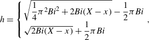 \begin{equation} h =\left \{ \begin{array}{l} \sqrt {\dfrac {1}{4}\pi ^2\textit{Bi}^2+2\textit{Bi}(X-x)}-\dfrac {1}{2}\pi \textit{Bi} \cr \sqrt {2\textit{Bi}(X-x)}+\dfrac {1}{2}\pi \textit{Bi} \end{array}\right ., \end{equation}
for horizontal compression or extension, respectively. Note that the profile in extension ends at $x=X$
with a finite depth (indicating an implausible vertical cliff face at the edge), and both profiles reduce to parameterless curves when using the variables,
$x=X$
with a finite depth (indicating an implausible vertical cliff face at the edge), and both profiles reduce to parameterless curves when using the variables, $(x,h)/\textit{Bi}$
. The predictions in (6.4) are added to figure 22(d,e) for comparison with the slipline solutions.
$(x,h)/\textit{Bi}$
. The predictions in (6.4) are added to figure 22(d,e) for comparison with the slipline solutions.
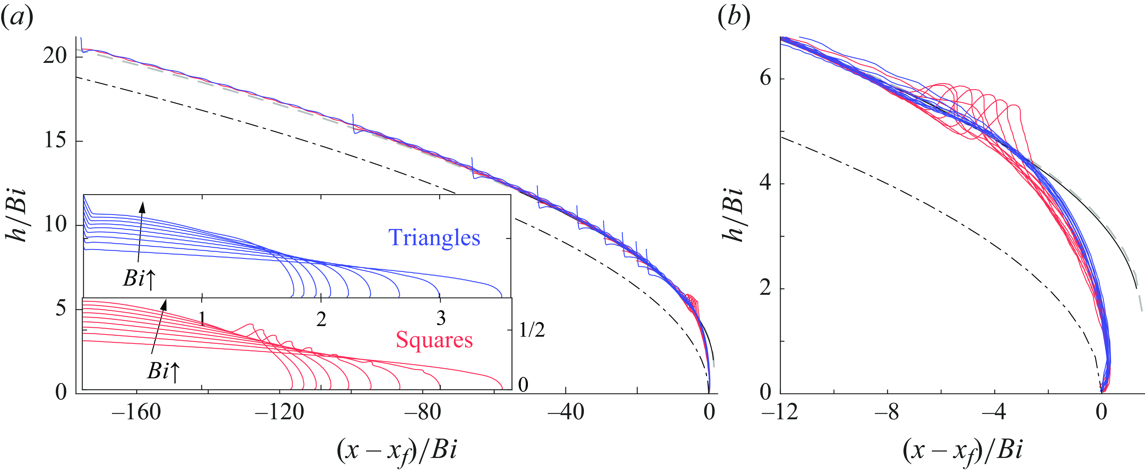
Figure 23. Final profiles from a suite of numerical simulations with varying $\textit{Bi}$
that begin with either a square or triangle of unit area (Liu et al. Reference Liu, Balmforth, Hormozi and Hewitt2016). The insets in (a) show the two sets of final profiles. These are then scaled by
$\textit{Bi}$
that begin with either a square or triangle of unit area (Liu et al. Reference Liu, Balmforth, Hormozi and Hewitt2016). The insets in (a) show the two sets of final profiles. These are then scaled by $\textit{Bi}$
and replotted in the main panel. A magnification near the front is displayed in (b). The dot-dashed line shows the leading-order asymptotic prediction from (6.3). The dashed line is the improved profile from (6.4) and the solid line shows the construction from figure 22(c). The latter two curves are shifted horizontally to align them with the numerical simulations at the position where
$\textit{Bi}$
and replotted in the main panel. A magnification near the front is displayed in (b). The dot-dashed line shows the leading-order asymptotic prediction from (6.3). The dashed line is the improved profile from (6.4) and the solid line shows the construction from figure 22(c). The latter two curves are shifted horizontally to align them with the numerical simulations at the position where $h=10\textit{Bi}$
.
$h=10\textit{Bi}$
.
Finally, the slipline results and higher-order asymptotic predictions for horizontal extension are replotted in figure 23 and compared with the final profiles from a suite of numerical simulations with varying $\textit{Bi}$
provided by Liu et al. (Reference Liu, Balmforth, Hormozi and Hewitt2016). These simulations are conducted by adopting either a square or triangular initial shape with the same area (the latter being a right-angle triangle with width
$\textit{Bi}$
provided by Liu et al. (Reference Liu, Balmforth, Hormozi and Hewitt2016). These simulations are conducted by adopting either a square or triangular initial shape with the same area (the latter being a right-angle triangle with width $\ell$
at the base, but height 2 at
$\ell$
at the base, but height 2 at $x=0$
). Aside from some relics from the initial shape, the final profiles are successfully collapsed on scaling by
$x=0$
). Aside from some relics from the initial shape, the final profiles are successfully collapsed on scaling by $\textit{Bi}$
. The scaled profiles match well with (6.4) and the slipline construction over distances exceeding about
$\textit{Bi}$
. The scaled profiles match well with (6.4) and the slipline construction over distances exceeding about $4\textit{Bi}$
(i.e. four times the dimensional length scale
$4\textit{Bi}$
(i.e. four times the dimensional length scale ${\tau _{_{_P}}}/(\rho g)$
). However, very close to the front, the latter terminate at finite height, whereas the simulations abruptly descend and bend around to create a small overhang. Evidently, (6.4) adequately describes the final shape of a slump except for the region at the nose, whose detailed structure remains unresolved.
${\tau _{_{_P}}}/(\rho g)$
). However, very close to the front, the latter terminate at finite height, whereas the simulations abruptly descend and bend around to create a small overhang. Evidently, (6.4) adequately describes the final shape of a slump except for the region at the nose, whose detailed structure remains unresolved.
7. Discussion: implications, complications and perspectives
7.1. Flow patterns; what to expect in the plastic limit
In the plastic limit, two-dimensional viscoplastic flow generates a patchwork of plugs, shear layers, wall boundary layers and regions of nearly perfectly plastic deformation. There is further substructure within the latter, guided by distinguished sliplines. The extent of the region of deformation is typically set by the length scale of the object acting as a forcing to or barrier against flow. Deformations can become more widespread if the forces needed to push fluid out of the way are not limited but become correspondingly higher as the volume of displaced fluid increases.
Driving flow by tangential motions of a wall can, in principle, be somewhat different, as the possibility then arises for all motion to be localised to a boundary layer. For example, in the limit of large rotation, the flow field around the translating and rotating cylinder of § 5.3 becomes localised to relatively narrow boundary layer at the surface (see Hewitt & Balmforth (Reference Hewitt and Balmforth2018)). However, as illustrated by the squirming cylinder (§ 5.4), deformation cannot always be confined within a wall boundary layer; weaker deformations are still driven plastically further afield. Other examples in which the deformation is not completely localised are provided by Oldroyd’s moving plate (Balmforth et al. Reference Balmforth, Craster, Hewitt, Hormozi and Maleki2017) and a swimming sheet driven by longitudinal waves (Hewitt & Balmforth Reference Hewitt and Balmforth2017). Therefore, it can be dangerous to conclude that remote deformations have an origin that is not viscoplastic.
Nevertheless, as illustrated by the translating and rotating cylinder, the addition of further motion components to a solid wall or translating object does not necessarily expand the yielded region. In fact, adding rotation (§ 5.3) or axial motion (5.5) to the translating cylinder initially leads to the same yielded area. Then, as one ramps up the rotation rate or axial speed, changes in flow pattern arise that actually decrease the yielded area. This somewhat counter-intuitive result might serve as a cautionary note in problems in which the goal is to eliminate plugs or enhance shear flow (such as in transport and mixing problems), where adding another component to the driving motion might seem advantageous.
The plastic limit also supports an interesting type of partial non-uniqueness: the same stress state is possible for different velocity fields. As the stress controls the yield surfaces, the geometrical shape of the flow pattern is the same. However, the streamlines, and the dissipation and its spatial structure, are different. For example, the solutions in figures 1, 10, 13(a), 15(a) and 16(c) all possess the Randolph–Houlsby stress field, but the streamlines and distribution of the shear rate are not the same. This non-uniqueness extends to problems with different boundary locations or shapes, or with isolated flow structures. In such cases, the intervening plugs provide effective cloaks to hide any detail embedded within them or lying further afield.
A related feature is that the velocity field associated with the checkerboards or circular fans of a slipline solution can be consistent with rigid-body motion. Certain velocity boundary conditions must be present for this to be the case, and if they are, the checkerboards or fans effectively plug up, even though the stress there is held exactly at the yield stress. With other velocity boundary conditions, however, shear must arise, implying that the checkerboards or fans appear as nearly plastic regions. We have termed the plugs that arise in the former setting as ‘serendipitous’ in view of this. The relatively low deformation rates associated with the plastic regions for $\textit{Bi}\gg 1$
also mean that viscous effects can sometimes eliminate shear at slightly smaller
$\textit{Bi}\gg 1$
also mean that viscous effects can sometimes eliminate shear at slightly smaller $\textit{Bi}$
. This leads to ‘residual’ plugs that owe their existence to finite viscosity and (somewhat counter-intuitively) are not present for
$\textit{Bi}$
. This leads to ‘residual’ plugs that owe their existence to finite viscosity and (somewhat counter-intuitively) are not present for $\textit{Bi}\to \infty$
. Therefore near the plastic limit, there can be three types of plugs, the last being the genuine, permanent plugs that feature in the slipline solution and truly lie below the yield stress.
$\textit{Bi}\to \infty$
. Therefore near the plastic limit, there can be three types of plugs, the last being the genuine, permanent plugs that feature in the slipline solution and truly lie below the yield stress.
One might wonder why the Randolph & Houlsby slipline pattern appears so prevalent in the solutions in § 5. Or, for that matter, why the components of Prandtl’s indentation solution are common in the solutions of § 4. One reason is that both have lines of symmetry, which imply that certain sliplines are straight. But Hencky’s rules then demand that a significant fraction of the slipline pattern must contain straight sliplines (§ 3.4). In combination with the geometry of a straight or circular boundary, the solution is thereby evidently forced to adopt those familiar forms.
A final curiosity is that the stress field can apparently be disfigured by discontinuities. Such scars are expected in the plastic limit (§ 3.4). But their appearance at finite Bingham number is, perhaps, a little shocking in view of the smoothing action of viscosity. In our numerical solutions, the discontinuities at finite $\textit{Bi}$
appear to be associated with ‘yield lines’. These are curves along which stresses reach the yield stress; on both sides, the yield criterion is met, so that the curves are not genuine yield surfaces. However, their appearance appears to allow the numerical solutions to establish stress jumps across the yield lines as the constitutive law no longer demands continuity there. We know of no results from analysis that preclude the existence of stress discontinuities at finite Bingham number (which, if they existed, would imply that those in figures 8 and 17 are numerical artefacts). We are also unaware of any previous computations, barring those in Hewitt & Balmforth (Reference Hewitt and Balmforth2017), that highlight their possible existence. Indeed, one imagines that such features are potentially problematic in numerical computations, requiring careful consideration to avoid persistent gridding errors and Gibbs phenomena.
$\textit{Bi}$
appear to be associated with ‘yield lines’. These are curves along which stresses reach the yield stress; on both sides, the yield criterion is met, so that the curves are not genuine yield surfaces. However, their appearance appears to allow the numerical solutions to establish stress jumps across the yield lines as the constitutive law no longer demands continuity there. We know of no results from analysis that preclude the existence of stress discontinuities at finite Bingham number (which, if they existed, would imply that those in figures 8 and 17 are numerical artefacts). We are also unaware of any previous computations, barring those in Hewitt & Balmforth (Reference Hewitt and Balmforth2017), that highlight their possible existence. Indeed, one imagines that such features are potentially problematic in numerical computations, requiring careful consideration to avoid persistent gridding errors and Gibbs phenomena.
7.2. Bifurcations; the role of stress inside the rigid plugs
A guiding principle of the inertialess problem in the plastic limit is that the solution must be a unique minimiser of the dissipation rate (for finite $\textit{Bi}$
, the quantity minimised is not quite this; see § 3.3). In other words, there cannot be multiple solutions with different values for
$\textit{Bi}$
, the quantity minimised is not quite this; see § 3.3). In other words, there cannot be multiple solutions with different values for $\mathcal{E}$
that correspond to local, but not global, minimisers. Therefore, when flow patterns changes at a point of bifurcation, one of the corresponding solutions must cease to exist, while the other must come into existence. In a number of situations, this demands that one or more plugs of the former must necessarily break to eliminate that pattern as a potential solution.
$\mathcal{E}$
that correspond to local, but not global, minimisers. Therefore, when flow patterns changes at a point of bifurcation, one of the corresponding solutions must cease to exist, while the other must come into existence. In a number of situations, this demands that one or more plugs of the former must necessarily break to eliminate that pattern as a potential solution.
This feature is not always obvious because the stress state within the plugs is indeterminate. The jet problem of § 4 provides numerous bifurcations that illustrate this point. The first bifurcation, for example, corresponds to the sudden breakage of the central, moving plug that, for smaller domain lengths, spans the entire domain (figure 4
c). But to determine when that plug breaks, one would need to track through every admissible stress field and demonstrate that all ceased to exist at the bifurcation point, an exercise that sounds impossible. A much better approach is to examine the solution after the bifurcation, with its broken plug and known stress state (i.e. Figure 4
d,e or figure 6
a), and then track that solution back to the bifurcation to gauge when that flow pattern must disappear. This exercise is certainly feasible and can be accomplished using the slipline solution in figure 6(a), which exists for $\ell _x \gt (1/4)\pi +(1/2)$
. The bifurcation point is thereby identified, and must correspond to the domain length at which the uninterrupted moving plug breaks. In other words, the analysis of the flow patterns at transitions is approached from one side only, taking a path that avoids the undetermined stress state of the plug that breaks. Alternatively, one might relax the treatment of the stress state below the yield stress, and use a constitutive law that predicts the plug stress. This is the approach implicitly taken when a regularised model is used, and would, in principle, allow a direct construction of the transition point from either side, were the solution to be analytically accessible.
$\ell _x \gt (1/4)\pi +(1/2)$
. The bifurcation point is thereby identified, and must correspond to the domain length at which the uninterrupted moving plug breaks. In other words, the analysis of the flow patterns at transitions is approached from one side only, taking a path that avoids the undetermined stress state of the plug that breaks. Alternatively, one might relax the treatment of the stress state below the yield stress, and use a constitutive law that predicts the plug stress. This is the approach implicitly taken when a regularised model is used, and would, in principle, allow a direct construction of the transition point from either side, were the solution to be analytically accessible.
Because the plugs that break at such a bifurcation have finite size, solution properties such as the yielded area can change discontinuously at transitions in flow pattern. The transitions of the jet at $\ell _x=(1/4)\pi +(1/2)$
and, for free-slip walls, at
$\ell _x=(1/4)\pi +(1/2)$
and, for free-slip walls, at $\ell _x\approx 1.9$
, for example, have this feature (see figure 4
b). We have referred to these types of transitions as ‘first order’, following the terminology of the theory of phase transition.
$\ell _x\approx 1.9$
, for example, have this feature (see figure 4
b). We have referred to these types of transitions as ‘first order’, following the terminology of the theory of phase transition.
Continuous, or ‘second-order’, types of transitions are also possible: in such cases, global solution properties like the yielded area do not abruptly change because the two flow patterns are connected continuously across the transition point by a common, nearly plastic (slipline) solution. For example, when the jet expands to meet the no-slip wall between panels (g) and (h) of figure 4, there is a connecting slipline field like that in figure 5(a). Since the boundary layer against a no-slip wall demands that sliplines intersect it tangentially, one expects transitions with this continuity whenever a yielded region or plug meets a no-slip boundary. Further examples are provided by the concentric annular problem in § 5.1 (see figure 10). By contrast, at a free-slip wall, or a line of symmetry, the slipline angle must be $\theta =(1/4)\pi$
. This rules out any continuous transition between slipline patterns when the yield region collides with the wall. Instead, there must be a sudden jump to a new flow pattern, with a breakage of one of the plugs; i.e. a first-order transition.
$\theta =(1/4)\pi$
. This rules out any continuous transition between slipline patterns when the yield region collides with the wall. Instead, there must be a sudden jump to a new flow pattern, with a breakage of one of the plugs; i.e. a first-order transition.
Such considerations impact the possibility for a plug to cloak a boundary or isolate a localised flowing region. For example, when a plug adheres to a no-slip boundary, that rigid material cloaks the wall to render its detailed shape and position irrelevant. Moreover, the plug will effectively cloak the boundary until stresses increase sufficiently for the yielded regions to progress smoothly to the wall; thereafter, a viscoplastic wall layer buffers the flow. For a free-slip wall or symmetry line, however, a sudden switch in flow state arises at an abrupt de-cloaking event, because the transition becomes first order. This points to the existence of long-range influence beyond the yielded envelope, or stress connections across bridging plugs. Beyond the examples considered here, such features have been explored in flow patterns around multiple particles moving through viscoplastic fluids (Chaparian et al. Reference Chaparian, Wachs and Frigaard2018).
7.3. Perspectives
Our aim here has been to gain insight into the impact of a fluid yield stress on flow structures and the dynamics, and our conclusions are perhaps best summarised by the bullet points in tables 1 and 2 presented in § 2. In order to explore these features, we have focused on three relatively simple problems involving the inertialess, two-dimensional flow of a Herschel–Bulkley fluid. Diving into more complicated modelling generally means leaving behind some of the ability to dissect and fully interpret solutions inherent in this ideal setting. However, although the relaxation of modelling assumptions inevitably renders the situation more murky, the intuition and general principles gained hopefully carry over into more complicated problems.
For example, it is not conceptually difficult to move from two to three dimensions, and there are many largely numerical (and experimental) studies that consider three-dimensional viscoplastic flows. Indeed, we have already looked into the effect of adding a component of flow in the third dimension in flow between concentric cylinders (§ 5.5), finding that aspects of the two-dimensional dynamics can survive. However, one key analytical tool is lost in the process: the slipline theory of perfect plasticity. It is also relatively straightforward, numerically, to incorporate inertia into viscoplastic modelling, although sufficiently strong inertial forces may well significantly disrupt the flow features identified here.
As noted in the introduction, most real viscoplastic materials violate the idealisations inherent in the Herschel–Bulkley model. In particular, most behave visco-elastically both below and above yield. Many recent studies of viscoplastic fluids employ an ‘elasto-viscoplastic’ formulation, with the most popular modelling approach following Saramito (Reference Saramito2007). Such studies have had success in capturing some of the experimental observations of yield-stress fluids that run counter to the predictions of non-elastic formulations (e.g. Fraggedakis, Dimakopoulos & Tsamopoulos (Reference Fraggedakis, Dimakopoulos and Tsamopoulos2016); Varchanis et al. (Reference Varchanis, Haward, Hopkins, Syrakos, Shen, Dimakopoulos and Tsamopoulos2020); Moschopoulos et al. (Reference Moschopoulos, Spyridakis, Varchanis, Dimakopoulos and Tsamopoulos2021); Esposito et al. (Reference Esposito, Dimakopoulos and Tsamopoulos2024)). While such elasto-viscoplastic models are now fairly commonly used in numerical studies, the anatomy of the flows produced are usually not dissected in quite the manner we have attempted here. This is partly because the added rheological complexity thwarts most analytical progress. It would, however, be instructive to explore in an idealised context and in a systematic manner how elasticity affects the canonical flow patterns discussed here. For example, can one quantify and interpret how elasticity affects the force balances that underpin the thin viscoplastic shear layers? In what manner do elastic forces act to disrupt the slipline structure of the extended plastic regions? Can one illustrate generic principles for how elasticity should affect the different types of plug?
Acknowledgements.
N.J.B. thanks the Isaac Newton Institute for Mathematical Sciences, Cambridge, for support and hospitality during the programme Anti-diffusive dynamics: from sub-cellular to astrophysical scales, where work on this paper was undertaken. This work was supported by EPSRC grant no EP/K032208/1.
Declaration of interests.
The authors report no conflict of interest.
Appendix A. Numerical details
A.1. Regularisation and the augmented Lagrangian method
The difficulties associated with numerically computing solutions to (3.6)–(3.9) include dealing with the rigid plugs and the associated indeterminacy of the stress. Practically, efforts that exploit the effective viscosity of the constitutive law are also plagued by its divergence at the yield surfaces. Both issues can be alleviated by abandoning the Herschel–Bulkley law in favour of a regularised version such as
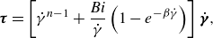 \begin{equation} \boldsymbol{\tau } = \left [{\dot \gamma }^{n-1} +\frac {\textit{Bi}}{{\dot \gamma }}\left (1-e^{-\beta {\dot \gamma }}\right )\right ] \dot {\boldsymbol{\gamma }}, \end{equation}
often known as the ‘Papanastasiou regularisation’ (Papanastasiou Reference Papanastasiou1987), where $\beta$
is a regularisation parameter that should be chosen to be sufficiently large that the yielded regions are insensitive to the precise choice for its value. More specifically,
$\beta$
is a regularisation parameter that should be chosen to be sufficiently large that the yielded regions are insensitive to the precise choice for its value. More specifically, $\beta ^{-1}$
represents a limiting scale for the strain rate
$\beta ^{-1}$
represents a limiting scale for the strain rate $\dot \gamma$
, below which the model inaccurately approximates the true Herschel–Bulkely law (3.3). There is no longer any need in (A1) for two branches to the constitutive law, nor the switch between them at the yield stress. Any true plug becomes replaced by a plug-like region with small strain rate and effective viscosity
$\dot \gamma$
, below which the model inaccurately approximates the true Herschel–Bulkely law (3.3). There is no longer any need in (A1) for two branches to the constitutive law, nor the switch between them at the yield stress. Any true plug becomes replaced by a plug-like region with small strain rate and effective viscosity $\sim \beta \textit{Bi}$
.
$\sim \beta \textit{Bi}$
.
Though popular, regularised models have the potentially unappealing feature of the removal of the true plugs. Other numerical approaches based on augmented Lagrangian algorithms are available that avoid this drawback. The trick is to augment the problem with some new variables and iterate to the solution; the extremum principles summarised above provide the formalism that underscores this strategy (see Treskatis et al. (Reference Treskatis, Roustaei, Frigaard and Wachs2018) for a concise and readable overview of modern approaches to this method).
For most of the two-dimensional numerical solutions presented here in the steady, inertialess, Bingham limit, we employ the following version of the augmented Lagrangian approach, which we outline in a practical manner, avoiding any derivation (for a more formal derivation, see Dean, Glowinski & Guidoboni (Reference Dean, Glowinski and Guidoboni2007); Glowinski & Wachs (Reference Glowinski and Wachs2011)). First, we take the curl of the force-balance equation (3.2) to eliminate the pressure, and enforce incompressibility by introducing a streamfunction such that
 \begin{align} \boldsymbol{u}=\left (\frac {\partial {\psi }}{\partial {y}},-\frac {\partial {\psi }}{\partial {x}}\right ) . \end{align}
The basic approach then is to introduce dummy tensors $\boldsymbol{d}$
and
$\boldsymbol{d}$
and $\boldsymbol{\lambda }$
, which are iterated towards the true strain rate
$\boldsymbol{\lambda }$
, which are iterated towards the true strain rate $\boldsymbol{{\dot \gamma }}$
and plastic stress
$\boldsymbol{{\dot \gamma }}$
and plastic stress $\textit{Bi} \boldsymbol{{\dot \gamma }}/{\dot \gamma }$
tensors, respectively. As such, these tensors each have only two independent components (the others being enforced by the symmetry and vanishing trace of the strain rate), which are iterated as follows, here illustrating the evolution from step
$\textit{Bi} \boldsymbol{{\dot \gamma }}/{\dot \gamma }$
tensors, respectively. As such, these tensors each have only two independent components (the others being enforced by the symmetry and vanishing trace of the strain rate), which are iterated as follows, here illustrating the evolution from step $k$
to step
$k$
to step $k+1$
:
$k+1$
:
 \begin{align} &\qquad\qquad\quad \begin{pmatrix} {\lambda ^{k+1}_{_{\textit{XX}}}} \\[5pt] {\lambda ^{k+1}_{_{\textit{XY}}}} \end{pmatrix} = \begin{pmatrix} {\lambda ^k_{_{\textit{XX}}}} \\[5pt] {\lambda ^k_{_{\textit{XY}}}} \end{pmatrix} + r \begin{pmatrix} 2\psi _{xx}^{k} \\[5pt] \psi _{yy}^{k}-\psi _{xx}^{k} \end{pmatrix} - r \begin{pmatrix} {d^k_{_{\textit{XX}}}} \\[5pt] {d^k_{_{\textit{XY}}}} \end{pmatrix}, \end{align}
 \begin{align} &\nabla ^4 \psi ^{k+1} = -\left(1 + r\right)^{-1} \left[ 2 \left({\lambda ^{k+1}_{_{\textit{XX}}}} - r {d^k_{_{\textit{XX}}}}\right)_{xy} + (\partial _{yy}-\partial _{xx})\left({\lambda ^{k+1}_{_{\textit{XY}}}} - r {d^k_{_{\textit{XY}}}}\right)\right], \end{align}
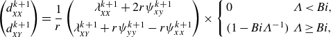 \begin{align} &\quad \begin{pmatrix} {d^{k+1}_{_{\textit{XX}}}} \\[5pt] {d^{k+1}_{_{\textit{XY}}}} \end{pmatrix} = \frac {1}{r} \begin{pmatrix} {\lambda ^{k+1}_{_{\textit{XX}}}} + 2r \psi ^{k+1}_{xy} \\[5pt] {\lambda ^{k+1}_{_{\textit{XY}}}} + r \psi ^{k+1}_{yy} - r \psi ^{k+1}_{xx} \end{pmatrix} \times \left \{ \begin{array}{ll} 0 & \Lambda \lt \textit{Bi}, \\[5pt] (1-\textit{Bi}\Lambda ^{-1}) & \Lambda \geq \textit{Bi}, \end{array}\right . \end{align}
with $\Lambda =\sqrt {4({\lambda ^{k+1}_{_{\textit{XX}}}} + 2r \psi ^{k+1}_{xy})^2 + ({\lambda ^{k+1}_{_{\textit{XY}}}} + r \psi ^{k+1}_{yy} - r \psi ^{k+1}_{xx})^2}$
and where
$\Lambda =\sqrt {4({\lambda ^{k+1}_{_{\textit{XX}}}} + 2r \psi ^{k+1}_{xy})^2 + ({\lambda ^{k+1}_{_{\textit{XY}}}} + r \psi ^{k+1}_{yy} - r \psi ^{k+1}_{xx})^2}$
and where $r = O(\textit{Bi})$
is a relaxation parameter. The superscripts indicate the iteration number, and the lower-case
$r = O(\textit{Bi})$
is a relaxation parameter. The superscripts indicate the iteration number, and the lower-case $(x,y)$
subscripts imply partial derivatives, as do the operators
$(x,y)$
subscripts imply partial derivatives, as do the operators $\partial _{xx}$
and
$\partial _{xx}$
and $\partial _{yy}$
. The iteration can be initiated with the Newtonian solution or an existing viscoplastic one, and converges to a solution with
$\partial _{yy}$
. The iteration can be initiated with the Newtonian solution or an existing viscoplastic one, and converges to a solution with $\boldsymbol{d}\equiv \boldsymbol{\dot \gamma }$
and
$\boldsymbol{d}\equiv \boldsymbol{\dot \gamma }$
and $\boldsymbol{\lambda } = \textit{Bi} \boldsymbol{\dot \gamma }/{\dot \gamma }$
over the yielded regions. Correspondingly, in the plugged regions
$\boldsymbol{\lambda } = \textit{Bi} \boldsymbol{\dot \gamma }/{\dot \gamma }$
over the yielded regions. Correspondingly, in the plugged regions $\boldsymbol{d} \to \boldsymbol{{\dot \gamma }} \to 0$
, while the augmented plastic stress tensor
$\boldsymbol{d} \to \boldsymbol{{\dot \gamma }} \to 0$
, while the augmented plastic stress tensor $\boldsymbol{\lambda }$
converges to an acceptable stress field there. Convergence is typically monitored by the magnitude of the difference between the dummy and true strain rates.
$\boldsymbol{\lambda }$
converges to an acceptable stress field there. Convergence is typically monitored by the magnitude of the difference between the dummy and true strain rates.
The true power of the technique is that the original nonlinear (and, indeed, non-differentiable) differential equations are replaced by solving the linear biharmonic relation in (A4) (which evaluates the yield-stress terms using a previous iterate, and locks in the boundary conditions as long as they can be expressed in terms of $\psi$
). The nonlinearity in the constitutive law is dealt with instead by (A5), which is simply an algebraic expression, with no more need to work with a potentially singular effective viscosity. The main downside of the approach is that convergence can be extremely slow, particularly in the plastic limit, and some care must be taken with accurate determination of convergence.
$\psi$
). The nonlinearity in the constitutive law is dealt with instead by (A5), which is simply an algebraic expression, with no more need to work with a potentially singular effective viscosity. The main downside of the approach is that convergence can be extremely slow, particularly in the plastic limit, and some care must be taken with accurate determination of convergence.
Note that the algorithm above is for a Bingham fluid; the Herschel–Bulkley version follows from replacing the factor $(1+r)^{-1}$
in (A4) with
$(1+r)^{-1}$
in (A4) with $(\mu ^* + r)^{-1}$
, where
$(\mu ^* + r)^{-1}$
, where $\mu ^* = \dot \gamma ^{n-1}$
is the dimensionless viscosity. However, if one desires to retain the linearity of the partial differential equation in (A4) (if the numerical solver requires this, for example), an alternative approach is to replace the factor
$\mu ^* = \dot \gamma ^{n-1}$
is the dimensionless viscosity. However, if one desires to retain the linearity of the partial differential equation in (A4) (if the numerical solver requires this, for example), an alternative approach is to replace the factor $(1+r)^{-1}$
with
$(1+r)^{-1}$
with $r^{-1}$
, and to replace the
$r^{-1}$
, and to replace the $1/r$
prefactor in (A5) by
$1/r$
prefactor in (A5) by $(\mu ^* + r)^{-1}$
. This approach places all the nonlinearity back into the algebraic equation (A5), leaving the elliptic problem linear; as a result, the dummy stress tensor
$(\mu ^* + r)^{-1}$
. This approach places all the nonlinearity back into the algebraic equation (A5), leaving the elliptic problem linear; as a result, the dummy stress tensor $\boldsymbol{\lambda }$
in this alternative formulation converges to the full deviatoric stress tensor
$\boldsymbol{\lambda }$
in this alternative formulation converges to the full deviatoric stress tensor $\boldsymbol{\lambda } \to (\textit{Bi}/\dot \gamma + \mu ^*) \boldsymbol{\dot \gamma }$
, rather than just to the plastic part of the stress.
$\boldsymbol{\lambda } \to (\textit{Bi}/\dot \gamma + \mu ^*) \boldsymbol{\dot \gamma }$
, rather than just to the plastic part of the stress.
A.2. Some practical numerical details
The numerical solutions presented here were computed using a mixed finite-difference approach that fundamentally replies on the linearity of the biharmonic equation in (A4). To begin, one spatial direction is identified in which the boundary conditions are amenable to a Fourier transform: a sine, cosine, or full transform can be employed to achieve odd, even, or periodic boundary conditions for the streamfunction and its derivatives. Having explicitly taken the transform, (A4) reduces to an ordinary differential equation that can be integrated using a standard finite-difference approach (requiring the inversion of a penta-diagonal matrix) before transforming the solution back to real space. The main strength of this approach is that it allows relatively accurate computations at high $\textit{Bi}$
: fast Fourier transforms render the method quite efficient, allowing for a fairly large number of grid cells and fairly small convergence tolerances in the augmented Lagrangian iteration scheme. Such accuracy is essential at high
$\textit{Bi}$
: fast Fourier transforms render the method quite efficient, allowing for a fairly large number of grid cells and fairly small convergence tolerances in the augmented Lagrangian iteration scheme. Such accuracy is essential at high $\textit{Bi}$
if one wants to accurately capture the finer details of, for example, narrow viscoplastic shear layers. In fact, it also turns out that high accuracy is often required to extract a reasonable map of slipline characteristics: although these features stretch across the extended plastic regions, they are sensitively affected by small changes in, for example, the pressure in the viscoplastic layers, which one might not otherwise notice was slightly inaccurate.
$\textit{Bi}$
if one wants to accurately capture the finer details of, for example, narrow viscoplastic shear layers. In fact, it also turns out that high accuracy is often required to extract a reasonable map of slipline characteristics: although these features stretch across the extended plastic regions, they are sensitively affected by small changes in, for example, the pressure in the viscoplastic layers, which one might not otherwise notice was slightly inaccurate.
The downsides of this numerical approach are its (lack of) versatility, particularly with respect to boundary conditions. For example, no-slip conditions on three walls of a rectangular domain is not straightforwardly achieved using this method. One way around that is to artificially construct a no-slip condition by dramatically enhancing the yield stress over a narrow ‘sponge layer’ adjacent to the boundary, which effectively forces the material to be plugged up there. This is the strategy adopted in § 4 to deal with no-slip boundaries at $y=\pm \ell _y$
, and it works effectively, although it slows down convergence of the algorithm somewhat.
$y=\pm \ell _y$
, and it works effectively, although it slows down convergence of the algorithm somewhat.
A final point relates to convergence, and the choice of the relaxation parameter $r$
in the scheme. We measure convergence by the proximity of the dummy strain rate
$r$
in the scheme. We measure convergence by the proximity of the dummy strain rate $\boldsymbol{d}$
and the true strain rate
$\boldsymbol{d}$
and the true strain rate $\boldsymbol{\dot \gamma } = \boldsymbol{\nabla u} + \boldsymbol{\nabla u}^T$
, with solutions being deemed to have converged when the average magnitude of the difference (that is, the mean root of the sum of the squares of the difference) lies below an imposed threshold. In most cases, we use a threshold of
$\boldsymbol{\dot \gamma } = \boldsymbol{\nabla u} + \boldsymbol{\nabla u}^T$
, with solutions being deemed to have converged when the average magnitude of the difference (that is, the mean root of the sum of the squares of the difference) lies below an imposed threshold. In most cases, we use a threshold of $O(10^{-7})$
, although in cases where the strain rates are themselves very low (as for the failure modes of § 6) it is more appropriate to use a relative error, and demand the relative error in
$O(10^{-7})$
, although in cases where the strain rates are themselves very low (as for the failure modes of § 6) it is more appropriate to use a relative error, and demand the relative error in $\boldsymbol{\dot \gamma }$
, scaled by the largest value of
$\boldsymbol{\dot \gamma }$
, scaled by the largest value of $\dot \gamma$
in the domain, is less than a given threshold (in § 6 we use a threshold of
$\dot \gamma$
in the domain, is less than a given threshold (in § 6 we use a threshold of $O(10^{-4})$
. This convergence metric is not the only choice: one could demand convergence pointwise, rather than in the mean, or could use a different metric (the simplest choice is simply to monitor the change in the strain rate between two iterates, and to require this to be sufficiently small; this is, however, an unsatisfactory measure, since the rate of change of the strain rate becoming small is no guarantee that the solution is close to convergence).
$O(10^{-4})$
. This convergence metric is not the only choice: one could demand convergence pointwise, rather than in the mean, or could use a different metric (the simplest choice is simply to monitor the change in the strain rate between two iterates, and to require this to be sufficiently small; this is, however, an unsatisfactory measure, since the rate of change of the strain rate becoming small is no guarantee that the solution is close to convergence).
More importantly, we find that the choice of relaxation parameter $r$
has a significant impact on convergence and the accuracy of solutions, a feature that may not be detected if one simply trusts that a given convergence criterion has been met. For example, it turns out that the boundary-layer profile against the ‘fake’ no-slip wall in figure 5(d) is sensitive to the choice of
$r$
has a significant impact on convergence and the accuracy of solutions, a feature that may not be detected if one simply trusts that a given convergence criterion has been met. For example, it turns out that the boundary-layer profile against the ‘fake’ no-slip wall in figure 5(d) is sensitive to the choice of $r$
, even though the flow structure elsewhere seems to be unchanged; values of
$r$
, even though the flow structure elsewhere seems to be unchanged; values of $r$
that are too large give increasingly inaccurate boundary-layer profiles, even at higher resolution. This feature could easily be missed without interrogation of the finer details, emphasising how numerical solutions near the plastic limit should be checked against theory whenever possible. Note that the alternative, but closely related, ‘dual-based proximal gradient’ algorithm (Treskatis et al. Reference Treskatis, Moyers-González and Price2016, Reference Treskatis, Roustaei, Frigaard and Wachs2018) may avoid this issue of choosing the relaxation parameter, as well as accelerating convergence.
$r$
that are too large give increasingly inaccurate boundary-layer profiles, even at higher resolution. This feature could easily be missed without interrogation of the finer details, emphasising how numerical solutions near the plastic limit should be checked against theory whenever possible. Note that the alternative, but closely related, ‘dual-based proximal gradient’ algorithm (Treskatis et al. Reference Treskatis, Moyers-González and Price2016, Reference Treskatis, Roustaei, Frigaard and Wachs2018) may avoid this issue of choosing the relaxation parameter, as well as accelerating convergence.
Appendix B. Plasticity details
A practical example of the construction of a slipline pattern is shown in figure 24, corresponding to one of the broken-jet flow patterns of § 4. The construction begins from a slipline that is known because a portion of the slipline field can be prescribed: the uniform inflow at the left-hand boundary corresponds to a checkerboard with $45^\circ$
sliplines. But the boundary condition implied by the checkerboard is inconsistent with no slip on the wall above and below the inflow. This inconsistency can be relieved by adding circular fans at the edges of the checkerboard. The resulting pattern mirrors Prandtl’s punch solution. Unlike in figure 2(b), however, we terminate the fan at a particular angle,
$45^\circ$
sliplines. But the boundary condition implied by the checkerboard is inconsistent with no slip on the wall above and below the inflow. This inconsistency can be relieved by adding circular fans at the edges of the checkerboard. The resulting pattern mirrors Prandtl’s punch solution. Unlike in figure 2(b), however, we terminate the fan at a particular angle, $ (1/2)\pi -\theta _{_E}$
, as illustrated on the left of figure 24. The upper fan then spans sliplines with
$ (1/2)\pi -\theta _{_E}$
, as illustrated on the left of figure 24. The upper fan then spans sliplines with $- (1/4)\pi \lt \theta \lt \theta _{_E}$
, and the angle
$- (1/4)\pi \lt \theta \lt \theta _{_E}$
, and the angle $\theta _{_E}$
becomes a parameter of the problem. The known starting slipline for the upper half of the solution is the final circular arc of the fan, the
$\theta _{_E}$
becomes a parameter of the problem. The known starting slipline for the upper half of the solution is the final circular arc of the fan, the $\beta -$
line
$\beta -$
line $AE$
(which has prescribed stress, up to an arbitrary pressure constant).
$AE$
(which has prescribed stress, up to an arbitrary pressure constant).
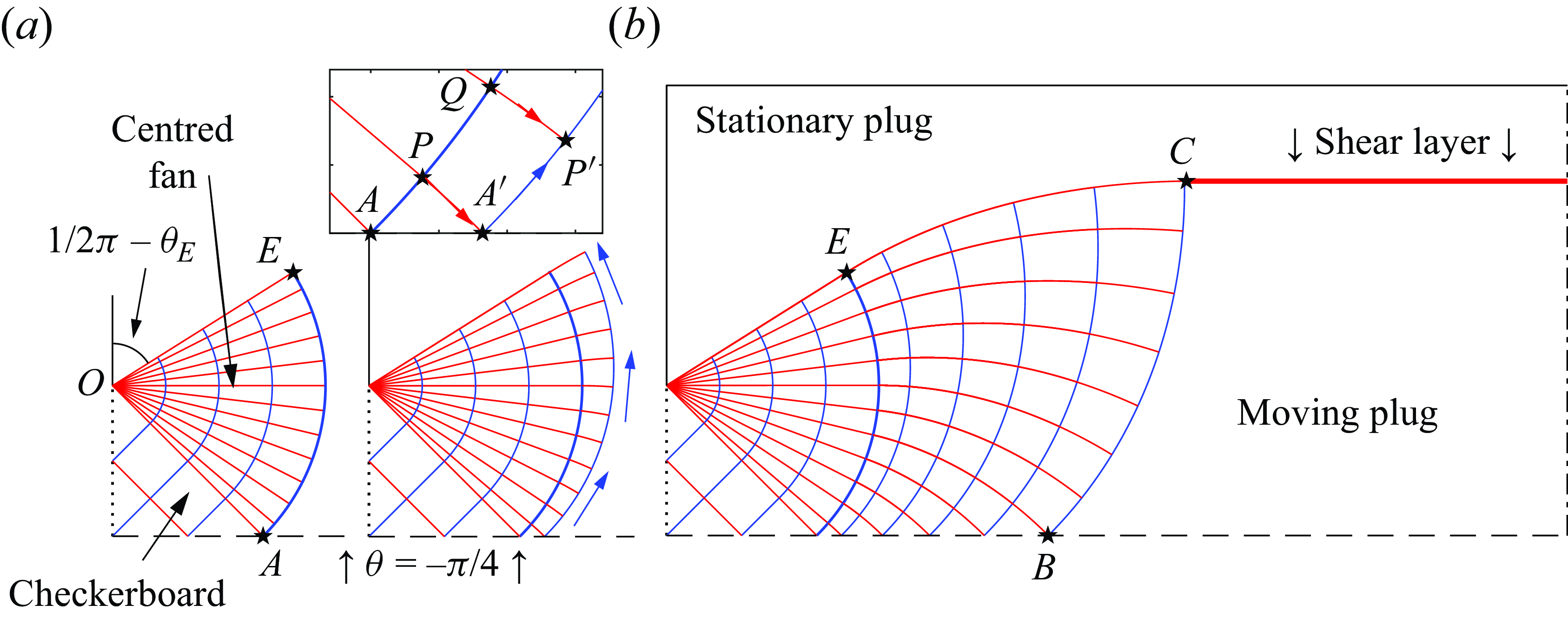
Figure 24. Illustration of the construction of a slipline network. We begin on the left with a piece of Prandtl’s punch solution: only half of the solution is displayed.
To construct the rest of the slipline field, we first extend the $\alpha $
-line that intersects point
$\alpha $
-line that intersects point $P$
along
$P$
along $AE$
down to the new point
$AE$
down to the new point $A'$
at
$A'$
at $y=0$
, as illustrated by the inset in the top left of figure 24. This extension is accomplished by combining the local slope of the
$y=0$
, as illustrated by the inset in the top left of figure 24. This extension is accomplished by combining the local slope of the $\alpha $
-line and its Riemann invariant with the symmetry condition
$\alpha $
-line and its Riemann invariant with the symmetry condition $\theta =-(1/4)\pi$
applying along
$\theta =-(1/4)\pi$
applying along $y=0$
. Specifically, using a simple finite-difference approximation (Hill Reference Hill1950; Prager & Hodge Reference Prager and Hodge1951), the new point
$y=0$
. Specifically, using a simple finite-difference approximation (Hill Reference Hill1950; Prager & Hodge Reference Prager and Hodge1951), the new point $A'$
is given by
$A'$
is given by $(x,y,\theta, p)=(x_{_P}-y_{_P}\cot ( ({1}/{2})\theta _{_P}-(1/4)\pi ),0, - (1/4)\pi, p_{_P}-2\textit{Bi}(\theta _{_P}+ (1/4)\pi ))$
, where the subscript refers values at point
$(x,y,\theta, p)=(x_{_P}-y_{_P}\cot ( ({1}/{2})\theta _{_P}-(1/4)\pi ),0, - (1/4)\pi, p_{_P}-2\textit{Bi}(\theta _{_P}+ (1/4)\pi ))$
, where the subscript refers values at point $P$
. The point
$P$
. The point $A'$
initiates a new
$A'$
initiates a new $\beta $
-line to the right of the fan. Similar finite-difference approximations allow one to advance this
$\beta $
-line to the right of the fan. Similar finite-difference approximations allow one to advance this $\beta $
-line from
$\beta $
-line from $A'$
to
$A'$
to $P'$
, combining the known characteristics information from
$P'$
, combining the known characteristics information from $A'$
and
$A'$
and $Q$
. Indeed, the entire new
$Q$
. Indeed, the entire new $\beta $
-line can be constructed by stepping up and along its length using the information from
$\beta $
-line can be constructed by stepping up and along its length using the information from $AE$
carried by the
$AE$
carried by the $\alpha $
-lines.
$\alpha $
-lines.
A repetition of this exercise furnishes the slipline field. The field terminates when the uppermost $\alpha $
-line becomes horizontal. At this point
$\alpha $
-line becomes horizontal. At this point $C$
, we must add the shear layer that extends across to the symmetry line at
$C$
, we must add the shear layer that extends across to the symmetry line at $x=\ell$
. At this stage, however,
$x=\ell$
. At this stage, however, $\ell$
cannot be prescribed. Instead, that length must be determined by evaluating the horizontal force along the rightmost
$\ell$
cannot be prescribed. Instead, that length must be determined by evaluating the horizontal force along the rightmost $\beta $
-line (from
$\beta $
-line (from $B$
to
$B$
to $C$
), and setting this force equal to
$C$
), and setting this force equal to $\textit{Bi}$
times the length of the shear layer (fixing
$\textit{Bi}$
times the length of the shear layer (fixing $\ell$
). This construction guarantees net force balance on the moving plug. The entire solution is thereby parameterised by the angle
$\ell$
). This construction guarantees net force balance on the moving plug. The entire solution is thereby parameterised by the angle $\theta _{_E}$
adopted at the outset.
$\theta _{_E}$
adopted at the outset.
B.1. Hencky’s rules
To quote Hencky’s rules, we first denote the radii of curvature of the two sliplines by
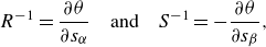 \begin{equation} R^{-1}=\frac {\partial \theta }{\partial s_\alpha } \quad \textrm {and} \quad S^{-1}=-\frac {\partial \theta }{\partial s_\beta }, \end{equation}
where $s_\alpha$
and
$s_\alpha$
and $s_\beta$
denote arclength along the
$s_\beta$
denote arclength along the $\alpha$
and
$\alpha$
and $\beta $
-lines, respectively. The rules are:
$\beta $
-lines, respectively. The rules are:
-
(i) For any curve of one of the family of sliplines, the change in the angle $\theta$
is constant between intersections with two adjacent lines of the other family. In other words, referring to figure 2, the change in the angle
$\theta$
between points
$A$
and
$C$
is the same as that between
$B$
and
$D$
(or the change in the angle along the
$\beta $
-lines
$AB$
and
$CD$
is the same).
$\theta$
is constant between intersections with two adjacent lines of the other family. In other words, referring to figure 2, the change in the angle
$\theta$
between points
$A$
and
$C$
is the same as that between
$B$
and
$D$
(or the change in the angle along the
$\beta $
-lines
$AB$
and
$CD$
is the same). -
(ii) As one traverses a slipline, the change in the radius of curvature of the other intersecting sliplines is equal to arc length
(B2)That is, in figure 2 as one progresses from
\begin{equation} \frac {\partial R}{\partial s_\beta } = \frac {\partial S}{\partial s_\alpha } = -1 . \end{equation}
$A$
to
$B$
, the radii of curvature of the
$\alpha -$
lines through
$A$
and
$B$
differ by the arclength of
$AB$
(or the radii of curvature of the
$\beta $
-lines at
$A$
and
$C$
differ by the arclength of
$AC$
).


B.2. Slipline calculations for figure 6
Over the upper fan, the pressure is constant along the $\alpha $
-lines (the radial spokes); along the circular
$\alpha $
-lines (the radial spokes); along the circular $\beta $
-lines, we have
$\beta $
-lines, we have
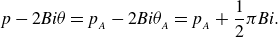 \begin{equation} p - 2\textit{Bi} \theta = p_{_A} - 2\textit{Bi} \theta _{_A} = p_{_A} + \frac {1}{2} \pi \textit{Bi} . \end{equation}
Thus,
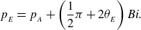 \begin{equation} p_{_E} = p_{_A} + \left(\frac {1}{2}\pi +2\theta _{_E}\right)\textit{Bi} . \end{equation}
Since $EC$
is an
$EC$
is an $\alpha $
-line
$\alpha $
-line
 \begin{equation} p_{_C} = p_{_E} + 2 (\theta _{_E} - \theta _{_C})\textit{Bi} = p_{_A} + \left(\frac {1}{2}\pi + 4\theta _{_E} - 2\theta _{_C} \right)\textit{Bi} . \end{equation}
Last, $BC$
is a
$BC$
is a $\beta $
-line, implying
$\beta $
-line, implying
 \begin{equation} p = p_{_C} + 2(\theta - \theta _{_C}) \textit{Bi} . \end{equation}
For the no-slip case in figure 6(a), point $C$
also lies along the horizontal shear layer. Here, the pressure variation is relatively small (§ C.1.1) and the symmetry condition at
$C$
also lies along the horizontal shear layer. Here, the pressure variation is relatively small (§ C.1.1) and the symmetry condition at $x=\ell _x$
demands that
$x=\ell _x$
demands that $p={\tau _{_{\textit{XX}}}}=0$
there. Thus,
$p={\tau _{_{\textit{XX}}}}=0$
there. Thus, $\theta _{_C}=p_{_C}=0$
, leaving
$\theta _{_C}=p_{_C}=0$
, leaving $p=2\theta \textit{Bi}$
along
$p=2\theta \textit{Bi}$
along $BC$
. The horizontal component of force along this curve is
$BC$
. The horizontal component of force along this curve is
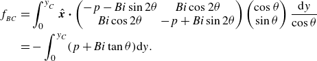 \begin{align} f_{_{BC}} &= \int _0^{y_{_C}} \hat {\boldsymbol{x}} \boldsymbol{\cdot } \begin{pmatrix} -p-\textit{Bi}\sin 2\theta & \textit{Bi}\cos 2\theta \cr \textit{Bi}\cos 2\theta & -p+\textit{Bi}\sin 2\theta \end{pmatrix} \begin{pmatrix} \cos \theta \cr \sin \theta \end{pmatrix} \frac {\textrm {d} y}{\cos \theta } \nonumber\\&= - \int _0^{y_{ C}} (p + \textit{Bi} \tan \theta ) \textrm {d} y. \end{align}
Because there can be no horizontal forces along $AB$
or the symmetry line
$AB$
or the symmetry line $x=\ell _x$
, this force component must be equal and opposite to that along the shear layer, which is
$x=\ell _x$
, this force component must be equal and opposite to that along the shear layer, which is $-\textit{Bi}(\ell _x-x_{_C})$
. It is this condition that dictates the position of point
$-\textit{Bi}(\ell _x-x_{_C})$
. It is this condition that dictates the position of point $C$
, given the domain length
$C$
, given the domain length $\ell _x$
and the slipline construction of
$\ell _x$
and the slipline construction of $\theta$
along
$\theta$
along $BC$
. In addition, by mass conservation, the speed of the moving plug at
$BC$
. In addition, by mass conservation, the speed of the moving plug at $BC$
is
$BC$
is $(2y_{_C})^{-1}$
, and the net dissipation rate (for
$(2y_{_C})^{-1}$
, and the net dissipation rate (for $y\gt 0$
) is
$y\gt 0$
) is
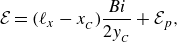 \begin{equation} \mathcal{E} = (\ell _x-x_{_C})\frac {\textit{Bi}}{2y_{_C}} + \mathcal{E}_p, \end{equation}
where $\mathcal{E}_p$
is the contribution from the upper plastic region. But this latter rate must also equal the net power input along the border
$\mathcal{E}_p$
is the contribution from the upper plastic region. But this latter rate must also equal the net power input along the border $OECBC$
, which is given by the input along
$OECBC$
, which is given by the input along $OA$
(and equal
$OA$
(and equal $-(1/2)(p_{_A}-\textit{Bi})$
) less the output along
$-(1/2)(p_{_A}-\textit{Bi})$
) less the output along $BC$
(given by
$BC$
(given by $f_{_{BC}} (2y_{_C})^{-1}$
). Altogether, and recalling that
$f_{_{BC}} (2y_{_C})^{-1}$
). Altogether, and recalling that $P_{_A}=-( (1/2)\pi +4\theta _{_E})\textit{Bi}$
when
$P_{_A}=-( (1/2)\pi +4\theta _{_E})\textit{Bi}$
when $P_{_C}=\theta _{_C}=0$
, we arrive at
$P_{_C}=\theta _{_C}=0$
, we arrive at
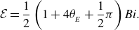 \begin{equation} \mathcal{E} = \frac {1}{2} \left(1 + 4\theta _{_E} + \frac {1}{2}\pi \right)\textit{Bi} . \end{equation}
Note that the upper slipline solution in figure 6(a) terminates when $\theta _{_E}\to 0$
,
$\theta _{_E}\to 0$
, $B\to A$
and
$B\to A$
and $C\to E$
. The force component
$C\to E$
. The force component $f_{_{BC}}$
can then be computed directly as
$f_{_{BC}}$
can then be computed directly as
 \begin{align} f_{_{BC}} \to \frac {1}{2}\textit{Bi} \left (1 - \sqrt 2 + \frac {1}{2}\pi \right ); \end{align}
( $p=2\theta \textit{Bi}$
along
$p=2\theta \textit{Bi}$
along $BC$
and
$BC$
and $\textrm {d} y= (1/2)\sqrt 2 \cos \theta \;\textrm {d}\theta$
). Force balance demands this be equal to
$\textrm {d} y= (1/2)\sqrt 2 \cos \theta \;\textrm {d}\theta$
). Force balance demands this be equal to $\textit{Bi}(\ell _x-x_{_C}) \to \textit{Bi}(\ell _x - ({1}/{2})\sqrt 2)$
, and so we find the bifurcation point
$\textit{Bi}(\ell _x-x_{_C}) \to \textit{Bi}(\ell _x - ({1}/{2})\sqrt 2)$
, and so we find the bifurcation point
 \begin{equation} \ell _x = \frac {1}{2} + \frac {1}{4}\pi . \end{equation}
For the free-slip case in figure 6(a), the position of point $C$
is set simply by the condition that
$C$
is set simply by the condition that $y_{_C}=\ell _y$
and
$y_{_C}=\ell _y$
and $\theta _{_C}= (1/4)\pi$
(
$\theta _{_C}= (1/4)\pi$
( $x_{_C}$
then following from the slipline construction). Moreover, the pressure
$x_{_C}$
then following from the slipline construction). Moreover, the pressure $p_{_C}$
cannot now vanish, but must be fixed by demanding that
$p_{_C}$
cannot now vanish, but must be fixed by demanding that $f_{_{BC}}=0$
, which follows because there are no other forces acting on the moving plug to the right of
$f_{_{BC}}=0$
, which follows because there are no other forces acting on the moving plug to the right of $C$
. i.e.
$C$
. i.e. $p=p_{_C} + (2\theta - (1/2)\pi ) \textit{Bi}$
along
$p=p_{_C} + (2\theta - (1/2)\pi ) \textit{Bi}$
along $BC$
, which must be fed into (B7) with
$BC$
, which must be fed into (B7) with $f_{_{BC}}=0$
, and then solved for
$f_{_{BC}}=0$
, and then solved for $p_{_C}$
. The only power input is now along
$p_{_C}$
. The only power input is now along $OA$
and so the net dissipation rate must be
$OA$
and so the net dissipation rate must be
 \begin{equation} \mathcal{E} = - \frac {1}{2}( p_{_A} - \textit{Bi}) = \frac {1}{2} (1 + 4 \theta _{_E}) \textit{Bi} - \frac {1}{2} p_{_C} . \end{equation}
B.3. Slipline calculations for figures 13 and 14
The slipline construction for the case without an upper fan in figure 13(c) was presented by Hewitt & Balmforth (Reference Hewitt and Balmforth2018); we summarise here the construction for the intermediate case in (b). To begin, consider the pressure along the contour $A_-B_-C_-C_+B_+A_+$
and its reflection in
$A_-B_-C_-C_+B_+A_+$
and its reflection in $x\lt 0$
. Let
$x\lt 0$
. Let $p_0$
denote the pressure at the bottom of the fan at
$p_0$
denote the pressure at the bottom of the fan at $A_-$
. The curve
$A_-$
. The curve $A_-B_-C_-$
is a
$A_-B_-C_-$
is a $\beta $
-line, and so
$\beta $
-line, and so
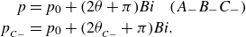 \begin{equation} \begin{aligned} p &= p_0 + (2\theta +\pi )\textit{Bi} \quad (A_-B_-C_-) \cr p_{_{C-}} &= p_0 + (2\theta _{_{C-}}+\pi ) \textit{Bi} . \end{aligned} \end{equation}
The combined section $C_-C_+B_+A_+$
is an
$C_-C_+B_+A_+$
is an $\alpha $
-line, implying
$\alpha $
-line, implying
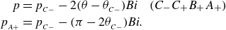 \begin{equation} \begin{aligned} p &= p_{_{C-}} - 2(\theta -\theta _{_{C-}})\textit{Bi} \quad (C_-C_+B_+A_+) \cr p_{_{A+}} &= p_{_{C-}} - (\pi -2\theta _{_{C-}})\textit{Bi} . \end{aligned} \end{equation}
Continuing the calculation around the mirror image in $x\lt 0$
, and finally returning to
$x\lt 0$
, and finally returning to $A_-$
, we find that the pressure is
$A_-$
, we find that the pressure is
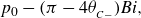 \begin{equation} p_0 - (\pi - 4\theta _{_{C-}})\textit{Bi}, \end{equation}
which should equal $p_0$
. Hence
$p_0$
. Hence $\theta _{_{C-}}= (1/4)\pi$
. Given that the disk’s motion can be viewed as pure rotation about the centre
$\theta _{_{C-}}= (1/4)\pi$
. Given that the disk’s motion can be viewed as pure rotation about the centre $E$
at
$E$
at $(0,\Omega ^{-1})$
the geometry of
$(0,\Omega ^{-1})$
the geometry of $EC_+$
and
$EC_+$
and $EC_-$
demands that these radial spokes have length
$EC_-$
demands that these radial spokes have length
 \begin{equation} R_{_{EC}} = \frac {1}{2} \left(\sqrt 2+\Omega ^{-1} \right). \end{equation}
To calculate the force and torque, consider the segment $O_-D_-C_-C_+D_+O_+$
(the net force and torque on the attached plug must vanish, and so contributions from
$O_-D_-C_-C_+D_+O_+$
(the net force and torque on the attached plug must vanish, and so contributions from $D_-C_-C_+D_+$
are the same as those along the plugged surface of the disk): if
$D_-C_-C_+D_+$
are the same as those along the plugged surface of the disk): if $\hat {\boldsymbol{n}}$
denotes the outward normal, each line element supports a force
$\hat {\boldsymbol{n}}$
denotes the outward normal, each line element supports a force
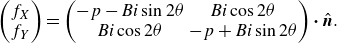 \begin{equation} \begin{pmatrix} f_{X} \cr f_{Y} \end{pmatrix} = \begin{pmatrix} -p-\textit{Bi}\sin 2\theta & \textit{Bi}\cos 2\theta \cr \textit{Bi}\cos 2\theta & -p+\textit{Bi}\sin 2\theta \end{pmatrix} \boldsymbol{\cdot } \hat {\boldsymbol{n}} . \end{equation}
The integral of $f_{X}$
along the various sections provides the net drag, whereas the integrals of
$f_{X}$
along the various sections provides the net drag, whereas the integrals of $f_{T} = xf_{Y}-yf_{X}$
determine the torque. The various contributions to the drag (setting
$f_{T} = xf_{Y}-yf_{X}$
determine the torque. The various contributions to the drag (setting $p_0=0$
, as the contribution of that background pressure ultimately cancels) are as follows:
$p_0=0$
, as the contribution of that background pressure ultimately cancels) are as follows:
 \begin{align} &\qquad\qquad O_-D_-: \quad \begin{aligned} \hat {\boldsymbol{n}}&=\begin{pmatrix}\sin \theta \cr -\cos \theta \end{pmatrix}, \cr 0&\lt \theta \lt \frac {1}{4}\pi, \end{aligned} \quad \frac {\delta F_{X}}{\textit{Bi}} = \frac {3\sqrt {2}}{4}(\pi -2)-\pi \\[-5pt] \nonumber \end{align}
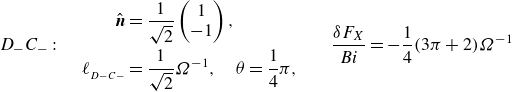 \begin{align} &\quad D_-C_-: \quad \begin{aligned} \hat {\boldsymbol{n}}&=\frac {1}{\sqrt 2}\begin{pmatrix}1\cr -1\end{pmatrix}, \cr \ell _{_{D-C-}}&=\frac {1}{\sqrt 2}\Omega ^{-1}, \quad \theta =\frac {1}{4}\pi, \end{aligned} \quad \frac {\delta F_{X}}{\textit{Bi}} = -\frac {1}{4}(3\pi +2)\Omega ^{-1} \\[-5pt] \nonumber \end{align}
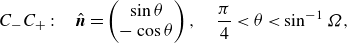 \begin{align} &\qquad\qquad\quad C_-C_+: \quad \hat {\boldsymbol{n}}=\begin{pmatrix}\sin \theta \cr -\cos \theta \end{pmatrix}, \quad \frac {\pi }{4}\lt \theta \lt \sin ^{-1}\Omega, \\[5pt] \nonumber \end{align}
 \begin{align} &\quad \frac {\delta F_{X}}{\textit{Bi}} = -\left(1+\frac {1}{\sqrt 2}\Omega ^{-1} \right)\left [\mbox{$\frac {3\pi }{2\sqrt 2}$} - \Omega + \frac {1}{\sqrt 2} - 2(\pi -\sin ^{-1}\Omega )\sqrt {1-\Omega ^2}\right ] \\[-5pt] \nonumber \end{align}
 \begin{align} & C_+D_+: \quad \hat {\boldsymbol{n}}=\begin{pmatrix}\sqrt {1-\Omega ^2}\cr \Omega \end{pmatrix}, \quad \ell _{_{C+D+}}=R_{_{EC}}-\sqrt {\Omega ^{-2}-1}, \quad \theta =\sin ^{-1}\Omega, \\[-5pt] \nonumber \end{align}
 \begin{align} &\qquad\quad \frac {\delta F_{X}}{\textit{Bi}} = - [1 + 2(\pi -\sin ^{-1}\Omega )\sqrt {\Omega ^{-2}-1}] [\Omega + \frac {1}{\sqrt 2} - \sqrt {1-\Omega ^2}] \\[-5pt] \nonumber \end{align}
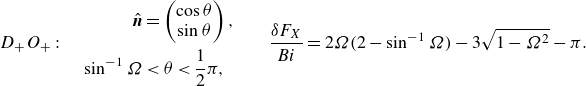 \begin{align} & D_+O_+: \quad \begin{aligned} \hat {\boldsymbol{n}}&=\begin{pmatrix}\cos \theta \cr \sin \theta \end{pmatrix}, \cr \sin ^{-1}\Omega &\lt \theta \lt \frac {1}{2}\pi, \end{aligned} \quad \frac {\delta F_{X}}{\textit{Bi}} = 2\Omega (2-\sin ^{-1}\Omega ) - 3\sqrt {1-\Omega ^2} - \pi . \end{align}
We avoid quoting the torque contributions as the formulae are somewhat cumbersome.
Summing the various contributions gives
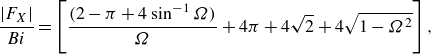 \begin{equation} \frac {|{F_{X}}|}{\textit{Bi}} = \left [\frac {(2-\pi +4\sin ^{-1}\Omega )}{\Omega } + 4\pi +4\sqrt 2+4\sqrt {1-\Omega ^2}\right ], \end{equation}
and
 \begin{equation} \frac {|T|}{\textit{Bi}} = \frac {1}{2}\Omega ^{-2} \left [\pi -2-2\pi \Omega ^2+4(2\Omega ^2-1)\sin ^{-1}\Omega +4\Omega \sqrt {1-\Omega ^2} \right ], \end{equation}
which bridge between the force and torque for Randolph & Houlsby’s solution in (5.4) and those for the slipline pattern in figure 13(c), which are (Hewitt & Balmforth Reference Hewitt and Balmforth2018)
 \begin{equation} \frac {|{F_{X}}|}{\textit{Bi}} = 2\pi +4\sqrt 2+\frac {2+3\pi }{\Omega } \quad \& \quad \frac {|T|}{\textit{Bi}} = 2\pi - \frac {3\pi +2}{2\Omega ^2}. \end{equation}
B.4. Including gravity and Nye’s construction of a glacier snout
When the body force of gravity acts, the slipline construction must be modified accordingly. First, we switch the pressure that appears in (3.15) to $P(x,y) = p(x,y) + (\rho g \mathcal{L}) y / \mathcal{P}$
, the non-hydrostatic part of the dimensionless pressure, assuming that gravity is directed in the negative
$P(x,y) = p(x,y) + (\rho g \mathcal{L}) y / \mathcal{P}$
, the non-hydrostatic part of the dimensionless pressure, assuming that gravity is directed in the negative $y$
-direction. The relations (3.15) still then apply, with the Riemann invariants along the sliplines modified to
$y$
-direction. The relations (3.15) still then apply, with the Riemann invariants along the sliplines modified to $P \pm 2\textit{Bi}\theta$
and the constructions of the slipline field proceeding otherwise as before. The only change with the addition of gravity is then to any boundary condition imposed on the stress, such as at a free surface.
$P \pm 2\textit{Bi}\theta$
and the constructions of the slipline field proceeding otherwise as before. The only change with the addition of gravity is then to any boundary condition imposed on the stress, such as at a free surface.
In that case of a free surface, the construction of the sliplines becomes more convoluted because the boundary position must be found as part of the solution of the problem. As part of this exercise, one hardwires the free-surface conditions into the construction of the slipline field, which requires that two families of sliplines meet the free surface at $45^\circ$
to the local tangent. For the slump problem, in which we choose
$45^\circ$
to the local tangent. For the slump problem, in which we choose $\mathcal{P} = \rho g \mathcal{H}$
and
$\mathcal{P} = \rho g \mathcal{H}$
and $\mathcal{L}=\mathcal{H}$
, one further demands
$\mathcal{L}=\mathcal{H}$
, one further demands $P=\textit{Bi}(h\pm 1)$
at the free surface
$P=\textit{Bi}(h\pm 1)$
at the free surface $y=h(x)$
, with the sign set by whether the final state is reached under horizontal compression or extension.
$y=h(x)$
, with the sign set by whether the final state is reached under horizontal compression or extension.
The alternative to Nye’s initial fan, that is used in figure 22(b), is the $\beta $
-line given by
$\beta $
-line given by
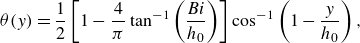 \begin{align} \theta (y) & = \frac {1}{2} \left [ 1 - \frac {4}{\pi }\tan ^{-1} \left (\frac {\textit{Bi}}{h_0}\right ) \right ] \cos ^{-1}\left (1-\frac {y}{h_0}\right ), \end{align}
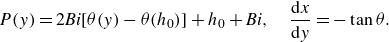 \begin{align} P(y) & = 2\textit{Bi}[\theta (y)-\theta (h_0)]+h_0+\textit{Bi}, \quad \frac {\textrm {d} x}{\textrm {d} y} = - \tan \theta . \end{align}
This choice recognises that the special solution to which Nye’s construction converges at larger depths is almost flat (and corresponds to that predicted by shallow-layer theory). The slipline therefore corresponds to one of Prandtl’s cyloids, but modified to allow for the small surface slope.
The inevitability of the bending downwards of the lowest $\alpha $
-line as the surface slope steepens (Nye Reference Nye1951) follows from Hencky’s rules: the combination of the surface boundary conditions and slipline equations imply that
$\alpha $
-line as the surface slope steepens (Nye Reference Nye1951) follows from Hencky’s rules: the combination of the surface boundary conditions and slipline equations imply that
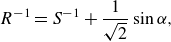 \begin{equation} R^{-1} = S^{-1} + \frac {1}{\sqrt 2}\sin \alpha, \end{equation}
for a point on the surface, where $\alpha =-\tan ^{-1}(h_x)$
gives the surface angle. For the
$\alpha =-\tan ^{-1}(h_x)$
gives the surface angle. For the $\alpha $
-line leaving the free surface at
$\alpha $
-line leaving the free surface at $G$
in figure 25(a),
$G$
in figure 25(a), $R\gt 0$
, but the upward
$R\gt 0$
, but the upward $\beta $
-line meeting this point has
$\beta $
-line meeting this point has $S\lt 0$
(as drawn,
$S\lt 0$
(as drawn, $\theta$
is increasing upwards). A short consideration of the geometry of the isosceles triangles formed by the slipline network just underneath the free surface, coupled with the pressure boundary condition, leads to (B30).
$\theta$
is increasing upwards). A short consideration of the geometry of the isosceles triangles formed by the slipline network just underneath the free surface, coupled with the pressure boundary condition, leads to (B30).
Now consider two adjacent $\beta $
-lines from the free surface to the bottom, labelled
$\beta $
-lines from the free surface to the bottom, labelled $GH$
and
$GH$
and $G'H'$
in the sketch shown in figure 25(a). Hencky’s first rule indicates that the
$G'H'$
in the sketch shown in figure 25(a). Hencky’s first rule indicates that the $\alpha $
-line intersecting the free surface at
$\alpha $
-line intersecting the free surface at $G$
must approach that point with the same sign for
$G$
must approach that point with the same sign for $R$
at that for the
$R$
at that for the $\alpha $
-line leaving the base at
$\alpha $
-line leaving the base at $H'$
(
$H'$
( $\theta$
changes by the same increment along both
$\theta$
changes by the same increment along both $\alpha $
-lines between their intersections with the two
$\alpha $
-lines between their intersections with the two $\beta $
-lines). Hencky’s second rule implies that
$\beta $
-lines). Hencky’s second rule implies that $S$
at
$S$
at $G$
must equal the length of the
$G$
must equal the length of the $\alpha $
-line
$\alpha $
-line $FG$
, because
$FG$
, because $S$
vanishes where the
$S$
vanishes where the $\beta $
-line hits the base at
$\beta $
-line hits the base at $F$
. As
$F$
. As $S^{-1}$
inevitably increases as we progress towards the nose of the current, but
$S^{-1}$
inevitably increases as we progress towards the nose of the current, but $({1}/{\sqrt 2})\sin \alpha$
is bounded, it follows from (B30) there must be a horizontal location at which
$({1}/{\sqrt 2})\sin \alpha$
is bounded, it follows from (B30) there must be a horizontal location at which $R$
for the top
$R$
for the top $\alpha $
-line (which was initially positive) becomes negative. The corresponding bottom
$\alpha $
-line (which was initially positive) becomes negative. The corresponding bottom $\alpha $
-line must therefore bend downwards.
$\alpha $
-line must therefore bend downwards.

Figure 25. Sliplines for horizontal (a) compression and (b) expansion, illustrating the geometry underlying Nye’s argument.
For horizontal extension, the slipline geometry illustrated in figure 25(b) implies that both $R$
and
$R$
and $S$
are positive (
$S$
are positive ( $\theta$
is now decreasing downwards, becoming less negative), and the construction leading to (B30) can be adjusted to now show that
$\theta$
is now decreasing downwards, becoming less negative), and the construction leading to (B30) can be adjusted to now show that
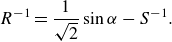 \begin{equation} R^{-1} = \frac {1}{\sqrt 2}\sin \alpha - S^{-1} . \end{equation}
Moreover, Hencky’s second rule still indicates that $S$
must equal the arclength of
$S$
must equal the arclength of $HG$
, which again becomes small if the slipline field extends down to
$HG$
, which again becomes small if the slipline field extends down to $h=0$
. Therefore,
$h=0$
. Therefore, $R^{-1}$
must again switch sign, both at the surface point (labelled
$R^{-1}$
must again switch sign, both at the surface point (labelled $G$
in figure 25
b), and at the base along the corresponding
$G$
in figure 25
b), and at the base along the corresponding $\beta -$
line (labelled
$\beta -$
line (labelled $H$
).
$H$
).
A simple alternative to Nye’s construction to build the slipline field under horizontal extension is to first set up a grid of heights $y=h$
along a section of the free surface, assign values of
$y=h$
along a section of the free surface, assign values of $\theta$
on the grid and then integrate
$\theta$
on the grid and then integrate
 \begin{equation} \frac {\textrm {d} x}{\textrm {d} h} = \cot \left(\theta +\frac {1}{4}\pi \right), \end{equation}
to obtain a free-surface shape. A network of sliplines can then be generated by integrating downwards to the heights $y_0$
where
$y_0$
where $\theta =0$
. Minimising the sum of squares of all the
$\theta =0$
. Minimising the sum of squares of all the $y_0$
’s (by, for example, using MATLAB’s fminsearch), one can then try to home in on the surface values of
$y_0$
’s (by, for example, using MATLAB’s fminsearch), one can then try to home in on the surface values of $\theta$
that lead to a slipline field which satisfies the true boundary condition (i.e.
$\theta$
that lead to a slipline field which satisfies the true boundary condition (i.e. $y_0=0$
). Constructions of this kind, beginning with guesses based on shallow-layer theory, appear in figure 22(b,f).
$y_0=0$
). Constructions of this kind, beginning with guesses based on shallow-layer theory, appear in figure 22(b,f).
Note that the profiles built in this fashion or by Nye’s construction do not constrain the total amount of material. Therefore, the only length scale of relevance is ${\tau _{_{_P}}}/(\rho g)$
. This implies that a simple rescaling of the problem is possible which eliminates all parameters. The rescaling is to take
${\tau _{_{_P}}}/(\rho g)$
. This implies that a simple rescaling of the problem is possible which eliminates all parameters. The rescaling is to take $L=H$
,
$L=H$
, $\textit{Bi}={\tau _{_{_P}}}/(\rho g H)$
, and then consider the new variables
$\textit{Bi}={\tau _{_{_P}}}/(\rho g H)$
, and then consider the new variables $\textit{Bi}^{-1}(x,y,h,p)$
, as used in figures 22 and 23.
$\textit{Bi}^{-1}(x,y,h,p)$
, as used in figures 22 and 23.
Appendix C. Asymptotic details
C.1. Viscoplastic boundary layers
C.1.1. Shear layers
When plastic slipline constructions are considered as the limit of a viscoplastic theory, any jump in tangential velocity across a slipline must be smoothed by viscosity over a narrow shear layer. Such viscoplastic shear layers were explored by Oldroyd (Reference Oldroyd1947b ), who gave a leading-order theory for their structure and offered a self-similar solution for the corresponding velocity profile. Because the shear layers follow sliplines, and such curves can also be yield surfaces, Oldroyd’s boundary layer can also act as the buffer between a plastically deforming region and a rigid plug. Indeed, it is also acceptable to place a shear layer between two plugs, in the manner of a line of failure between rigid blocks.
Oldroyd’s original shear-layer theory considered a straight boundary layer within a Bingham fluid. His analysis was generalised by Balmforth et al. (Reference Balmforth, Craster, Hewitt, Hormozi and Maleki2017) to allow for a curved centreline (i.e. centring slipline) and fluid described by the Herschel–Bulkley law. In this generalisation, the curvilinear coordinate system $(s,\eta )$
of § 3.2 is defined by the centreline of the shear layer (i.e. the slipline at the shear layer’s centre has
$(s,\eta )$
of § 3.2 is defined by the centreline of the shear layer (i.e. the slipline at the shear layer’s centre has $s=s_\alpha$
or
$s=s_\alpha$
or $s=s_\beta$
and
$s=s_\beta$
and $\eta =0$
).
$\eta =0$
).
When the shear layer is relatively thin (compared with its length), the geometry demands that $V\ll U$
,
$V\ll U$
, ${\dot \gamma _{_{\textit{SS}}}}\sim 2U_s$
and
${\dot \gamma _{_{\textit{SS}}}}\sim 2U_s$
and ${\dot \gamma _{_{SN}}}\sim U_\eta$
where we have used subscripts corresponding to the spatial coordinates(
${\dot \gamma _{_{SN}}}\sim U_\eta$
where we have used subscripts corresponding to the spatial coordinates( $s,\eta$
) as a shorthand for partial derivatives (an exercise we extend to the Cartesian coordinates (x, y) and time t below). In Oldroyd’s theory the main balances of terms from (3.6) are
$s,\eta$
) as a shorthand for partial derivatives (an exercise we extend to the Cartesian coordinates (x, y) and time t below). In Oldroyd’s theory the main balances of terms from (3.6) are
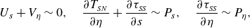 \begin{equation} U_s + V_\eta \sim 0, \quad \frac {\partial {{T_{_{SN}}}}}{\partial {\eta }} + \frac {\partial {{\tau _{_{\textit{SS}}}}}}{\partial {s}} \sim P_s, \quad \frac {\partial {{\tau _{_{\textit{SS}}}}}}{\partial {\eta }} \sim P_\eta, \end{equation}
where
 \begin{equation} p = -2\sigma \textit{Bi} \theta + P, \!\!\!\quad {\tau _{_{SN}}} = \sigma \textit{Bi} + {T_{_{SN}}}, \!\!\!\quad {\tau _{_{\textit{SS}}}} \sim \frac {2\sigma \textit{Bi} U_s}{U_\eta }, \!\!\!\quad {T_{_{SN}}} \sim |U_\eta |^{n-1} U_\eta - \frac {2\sigma \textit{Bi} U_s^2}{U_\eta ^2}, \end{equation}
and $\sigma =+1$
(
$\sigma =+1$
( $\sigma =-1$
) if
$\sigma =-1$
) if $U_\eta \gt 0$
(
$U_\eta \gt 0$
( $U_\eta \lt 0$
). The leading-order part of the pressure (
$U_\eta \lt 0$
). The leading-order part of the pressure ( $-2\sigma \textit{Bi}\theta$
) is demanded by the Riemann invariant of the slipline threading the shear layer (recall
$-2\sigma \textit{Bi}\theta$
) is demanded by the Riemann invariant of the slipline threading the shear layer (recall $\kappa =\theta _s$
), which is an
$\kappa =\theta _s$
), which is an $\alpha $
-line (
$\alpha $
-line ( $\beta$
-line) if
$\beta$
-line) if $\sigma =+1$
(
$\sigma =+1$
( $\sigma =-1$
). Because the leading-order term in the stress tensor is constant (
$\sigma =-1$
). Because the leading-order term in the stress tensor is constant ( ${\tau _{_{SN}}}\sim \sigma \textit{Bi}$
and
${\tau _{_{SN}}}\sim \sigma \textit{Bi}$
and $|{T_{_{SN}}}|\ll \textit{Bi}$
), and all the terms from the curvature of the shear layer cancel to leading order, force balance boils down to countering pressure gradients with a mix of the viscous shear stress and higher-order plastic stress corrections.
$|{T_{_{SN}}}|\ll \textit{Bi}$
), and all the terms from the curvature of the shear layer cancel to leading order, force balance boils down to countering pressure gradients with a mix of the viscous shear stress and higher-order plastic stress corrections.
The leading-order relations in (C1)–(C2) can be combined into Oldroyd’s shear-layer equation, which is the formidable-looking partial differential equation
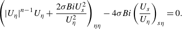 \begin{equation} \left ( |U_\eta |^{n-1} U_\eta + \frac {2\sigma \textit{Bi} U_s^2}{U_\eta ^2} \right )_{\eta \eta } - 4 \sigma \textit{Bi} \left ( \frac {U_s}{U_\eta }\right )_{s\eta } = 0. \end{equation}
This equation must be solved subject to matches of $U$
to the flow to either side of the shear layer:
$U$
to the flow to either side of the shear layer: $U\to U_\pm$
for
$U\to U_\pm$
for $\eta \to \pm \sigma \textit{Bi}^{-1/(n+2)}Y(s)$
, where
$\eta \to \pm \sigma \textit{Bi}^{-1/(n+2)}Y(s)$
, where $U_+-U_-$
(with
$U_+-U_-$
(with $U_+\gt U_-$
) is the jump in tangential velocity across the shear layer and its half-width is
$U_+\gt U_-$
) is the jump in tangential velocity across the shear layer and its half-width is $\textit{Bi}^{-1/(n+2)}Y(s)$
.
$\textit{Bi}^{-1/(n+2)}Y(s)$
.
Despite the daunting look of (C3), that equation has a useful self-similar solution in which
 \begin{equation} U(s,\eta ) = \frac {1}{2} (U_++U_-) + (U_+-U_-) f(\zeta ), \quad \zeta = \sigma \textit{Bi}^{1/(n+2)} \frac {\eta }{Y(s)} . \end{equation}
The profile function $f(\zeta )$
is given by an incomplete beta function, and the shear-layer half-width
$f(\zeta )$
is given by an incomplete beta function, and the shear-layer half-width $Y(s)$
follows from solving a relatively simple ordinary differential equation (Balmforth et al. Reference Balmforth, Craster, Hewitt, Hormozi and Maleki2017). For Bingham fluids (
$Y(s)$
follows from solving a relatively simple ordinary differential equation (Balmforth et al. Reference Balmforth, Craster, Hewitt, Hormozi and Maleki2017). For Bingham fluids ( $n=1$
), the solution is more transparent and given by
$n=1$
), the solution is more transparent and given by
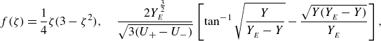 \begin{equation} f(\zeta )=\frac 14 \zeta (3-\zeta ^2), \quad \frac {2Y_{_E}^{\frac 32} }{\sqrt {3(U_+-U_-)}} \left [ \tan ^{-1}\sqrt {\frac {Y}{Y_{_E}-Y}} - \frac {\sqrt {Y (Y_{_E}-Y)}}{Y_{_E}} \right ], \end{equation}
if the boundary opens at $s=0$
(so
$s=0$
(so $Y(0)=0$
) and reaches a maximum half-width of
$Y(0)=0$
) and reaches a maximum half-width of $\textit{Bi}^{-1/3}Y_{_E}=\textit{Bi}^{-1/3}Y(s_{_E})$
at
$\textit{Bi}^{-1/3}Y_{_E}=\textit{Bi}^{-1/3}Y(s_{_E})$
at
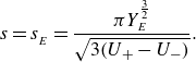 \begin{equation} s = s_{_E} = \frac {\pi Y_{_E}^{\frac 32}}{\sqrt {3(U_+-U_-)}} . \end{equation}
That is, the maximum half-width and length are related by
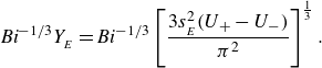 \begin{equation} \textit{Bi}^{-1/3}Y_{_E} = \textit{Bi}^{-1/3}\left [\frac {3s_{_E}^2(U_+-U_-)}{\pi ^2}\right ]^{\frac 13} . \end{equation}
Further calculations imply that the area occupied by the shear layer is
 \begin{equation} 2 \textit{Bi}^{-1/3} \int _0^{s_{_E}} Y(s) \; \textrm {d} s = \frac {3}{2}\pi ^{-2/3} s_{_E}^{5/3} \textit{Bi}^{-1/3} [3(U_+-U_-]^{1/3}, \end{equation}
and, to leading order, the net dissipation rate arising over it is given by
 \begin{equation} \mathcal{E} \sim (U_+-U_-)s_{_E}\textit{Bi}. \end{equation}
The results in (C5), (C8) and (C9), with $(U_+,U_-)=(1,0)$
and
$(U_+,U_-)=(1,0)$
and $s\equiv x$
, are compared with numerical solutions for the jet problem in figures 4 and 5 (
$s\equiv x$
, are compared with numerical solutions for the jet problem in figures 4 and 5 ( $s_{_E}\to \ell _x$
), and for the translating disk in figure 1(d).
$s_{_E}\to \ell _x$
), and for the translating disk in figure 1(d).
C.1.2. Wall layers
Viscoplastic boundary layers can also arise against a no-slip wall. In such settings, the wall need not align with a slipline and the flow structure is necessarily different (Beris et al. Reference Beris, Tsamopoulos, Armstrong and Brown1985; Piau Reference Piau2002; Balmforth et al. Reference Balmforth, Craster, Hewitt, Hormozi and Maleki2017). The main balances in the boundary layer follow those in Reynolds lubrication theory
 \begin{equation} U_s+V_\eta \sim 0, \quad \frac {\partial {\tau _{_{SN}}}}{\partial \eta } - 2 \kappa {\tau _{_{SN}}} \sim p_s, \quad 0 \sim p_\eta . \end{equation}
i.e. the pressure is approximately constant across the boundary layer and its gradient along the layer balances the resistance from shear stresses. Hence, taking $\eta$
to increase into the fluid from the wall at
$\eta$
to increase into the fluid from the wall at $\eta =0$
,
$\eta =0$
,
 \begin{equation} p \sim P(s) \quad \& \quad {\tau _{_{SN}}} \sim \sigma \textit{Bi} + (\eta - \eta _*) (P_s+2\kappa \sigma \textit{Bi}), \end{equation}
where $\sigma =$
sgn
$\sigma =$
sgn $(U_\eta )$
and
$(U_\eta )$
and $\eta =\eta _*$
denotes the edge of the boundary layer, at which location the stress invariant, which is dominated by
$\eta =\eta _*$
denotes the edge of the boundary layer, at which location the stress invariant, which is dominated by $\tau _{_{SN}}$
, must decrease towards the yield stress. Given that the boundary layer is thin,
$\tau _{_{SN}}$
, must decrease towards the yield stress. Given that the boundary layer is thin, $\eta \ll 1$
, and so the first term in the shear stress in (C11) significantly outweighs the second.
$\eta \ll 1$
, and so the first term in the shear stress in (C11) significantly outweighs the second.
The leading-order form of the constitutive law demands that
 \begin{equation} {\tau _{_{SN}}} \sim \sigma \textit{Bi} + |U_\eta |^{n-1} U_\eta, \end{equation}
which, in combination with (C11), leads to the velocity profile
 \begin{equation} U \sim U_w - \frac {n}{n+1}\left |P_s+2\kappa \sigma \textit{Bi}\right |^{\frac 1n} \left[|\eta _*|^{1+\frac 1n} - |\eta _*-\eta |^{1+\frac 1n} \right] \; \textrm {sgn}(P_s+2\kappa \sigma \textit{Bi}), \end{equation}
given that sgn $(U_\eta )\equiv -$
sgn
$(U_\eta )\equiv -$
sgn $(P_s+2\kappa \sigma \textit{Bi})\,\times$
sgn
$(P_s+2\kappa \sigma \textit{Bi})\,\times$
sgn $(\eta _*)$
. Here,
$(\eta _*)$
. Here, $U(s,0)=U_w$
is the tangential wall velocity. If
$U(s,0)=U_w$
is the tangential wall velocity. If $U=U_*$
at
$U=U_*$
at $\eta =\eta _*$
, then we find that the velocity jump is related to the pressure gradient and boundary-layer thickness by
$\eta =\eta _*$
, then we find that the velocity jump is related to the pressure gradient and boundary-layer thickness by
 \begin{equation} U_*-U_w \sim -\frac {n}{n+1}\left |P_s+2\kappa \sigma \textit{Bi}\right |^{\frac 1n} |\eta _*|^{1+\frac 1n} \; \textrm {sgn}(P_s+2\kappa \sigma \textit{Bi}) . \end{equation}
A further relation arises from mass conservation: the net flux along the layer is
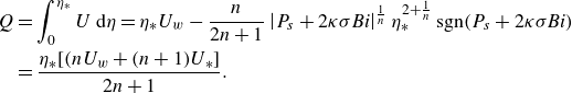 \begin{align} Q &= \int _0^{\eta _*} U \; \textrm {d}\eta = \eta _* U_w -\frac {n}{2n+1} \left |P_s +2\kappa \sigma \textit{Bi} \right |^{\frac 1n} \eta _*^{2+\frac 1n} \; \textrm {sgn}(P_s+2\kappa \sigma \textit{Bi}) \nonumber \\ &= \frac {\eta _* [(nU_w + (n+1)U_*]}{2n+1} . \end{align}
But
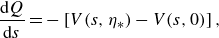 \begin{equation} \frac {\textrm {d} Q}{\textrm {d} s} = - \left [ V(s,\eta _*) - V(s,0) \right ], \end{equation}
or
 \begin{equation} \frac {\eta _* [(nU_w + (n+1)U_*]}{2n+1} = Q_0 - \int _0^s \left [ V(s,\eta _*) - V(s,0) \right ] \; \textrm {d} s, \end{equation}
for some flux constant $Q_0$
. To proceed any further, the normal velocities or pressure drop along the boundary layer must be specified, which requires a splice with the surrounding flow. In most situations, this splice demands that
$Q_0$
. To proceed any further, the normal velocities or pressure drop along the boundary layer must be specified, which requires a splice with the surrounding flow. In most situations, this splice demands that $P=O(\textit{Bi})$
(in the plastic limit). It follows that the boundary layer has a characteristic thickness given by
$P=O(\textit{Bi})$
(in the plastic limit). It follows that the boundary layer has a characteristic thickness given by
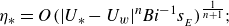 \begin{equation} \eta _* = O( |U_*-U_w|^n \textit{Bi}^{-1} s_{_E})^{\frac {1}{n+1}}; \end{equation}
(where $s_{_E}$
is again the boundary-layer length), which is thinner than Oldroyd’s shear layer (which has a thickness of
$s_{_E}$
is again the boundary-layer length), which is thinner than Oldroyd’s shear layer (which has a thickness of $O(\textit{Bi}^{-1/(n+2)})$
).
$O(\textit{Bi}^{-1/(n+2)})$
).
C.1.3. Flat plate next to a moving plug
When the boundary layer buffers a straight wall from a plug, the tangential velocity jump $U_*-U_w$
is constant and the normal velocity
$U_*-U_w$
is constant and the normal velocity $V$
vanishes on both sides. The net flux
$V$
vanishes on both sides. The net flux $Q$
must then be constant, demanding that the boundary layer have uniform thickness and pressure gradient. The velocity profile becomes
$Q$
must then be constant, demanding that the boundary layer have uniform thickness and pressure gradient. The velocity profile becomes
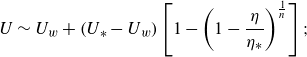 \begin{equation} U \sim U_w + (U_*-U_w) \left [1 - \left (1 - \frac {\eta }{\eta _*}\right )^{\frac 1n}\right ]; \end{equation}
(cf. figure 5 b,d; the corresponding profile for the translating disk is compared with numerical results in figure 1 e).
C.1.4. Boundary-layered squirmers
For a Bingham fluid ( $n=1$
) between a circular wall with unit radius and a surrounding stationary plug, we have
$n=1$
) between a circular wall with unit radius and a surrounding stationary plug, we have
 \begin{equation} s \equiv \phi, \quad \eta = -(r-1), \quad \kappa = 1, \quad U_*=0, \quad \sigma = \textrm {sgn}(U_w). \end{equation}
The boundary-layer profile simplifies to
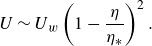 \begin{equation} U \sim U_w \left ( 1 - \frac {\eta }{\eta _*} \right )^2 . \end{equation}
Since the wall speed is specified, $U_w = {U_{W}}(\phi ) + O(\textit{Bi}^{-1/2})$
, we solve (C14) for the pressure gradient
$U_w = {U_{W}}(\phi ) + O(\textit{Bi}^{-1/2})$
, we solve (C14) for the pressure gradient
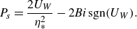 \begin{equation} P_s = \frac {2 {U_{W}}}{\eta _*^2} - 2 \textit{Bi} \; \textrm {sgn}({U_{W}}). \end{equation}
Given that $V(s,0)={u_{W}}\cos \phi$
and
$V(s,0)={u_{W}}\cos \phi$
and $V(s,\eta _*)=0$
, the flux relation in (C17) reduces to
$V(s,\eta _*)=0$
, the flux relation in (C17) reduces to
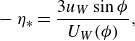 \begin{equation} -\eta _* = \frac {3{u_{W}}\sin \phi }{{U_{W}}(\phi )}, \end{equation}
since ${U_{W}}(0)=0$
(eliminating the integration constant
${U_{W}}(0)=0$
(eliminating the integration constant $Q_0$
). Evidently,
$Q_0$
). Evidently, ${U_{W}}(\phi )$
must have the same sign as
${U_{W}}(\phi )$
must have the same sign as $\sin \theta$
(
$\sin \theta$
( $\eta _*\lt 0$
); otherwise the boundary layer cannot contain the flow.
$\eta _*\lt 0$
); otherwise the boundary layer cannot contain the flow.
Since the pressure $P$
and shear stress
$P$
and shear stress ${\tau _{_{R\Phi }}}=-{\tau _{_{SN}}}\sim -\textit{Bi}$
sgn
${\tau _{_{R\Phi }}}=-{\tau _{_{SN}}}\sim -\textit{Bi}$
sgn $({U_{W}})$
dominate the stress at
$({U_{W}})$
dominate the stress at $\eta =0$
, the net force on the squirmer can be evaluated as
$\eta =0$
, the net force on the squirmer can be evaluated as
 \begin{equation} {F_{X}} \sim 2 \int _0^\pi [\textit{Bi}\;\textrm {sgn}({U_{W}}) \sin \phi - P\cos \phi ] \; \textrm {d} \phi = \frac {4}{9{u^2_{W}}} \int _0^\pi \frac {|{U_{W}}|^3\; \textrm {d} \phi }{\sin \phi } - 4 \textit{Bi} . \end{equation}
Finally, because the tangential velocity gradient across the boundary layer again dominates the shear rate tensor, the net dissipation rate is given by (5.5).
C.2. Lubrication theory
If the geometry of the flow domain takes the form a narrow gap, then Reynolds lubrication analysis applies throughout. The reduction of the problem becomes complicated, however, by the fact that a number of different flow patterns are possible depending on the applied stresses (Hewitt & Balmforth Reference Hewitt and Balmforth2012). As an example (although one for which this full richness is not realised), we consider a narrow gap of uniform thickness $h$
in which flow is driven by primarily the normal motion of one of the walls; i.e. a squeeze flow like that considered in § 5.2.
$h$
in which flow is driven by primarily the normal motion of one of the walls; i.e. a squeeze flow like that considered in § 5.2.
Returning to (C10) (which again applies), we now write
 \begin{equation} {\tau _{_{SN}}} \sim \left(\eta -\frac {1}{2} h \right)P_s, \end{equation}
because the velocity boundary conditions $U(s,0)=U(s,h)=0$
imply symmetry about the midline of the gap. That said, a key difference with the solution (C11) adopted in § C.1.2 is that lubrication pressures are relatively large
$U(s,0)=U(s,h)=0$
imply symmetry about the midline of the gap. That said, a key difference with the solution (C11) adopted in § C.1.2 is that lubrication pressures are relatively large $P\gg \textit{Bi}$
, leading us to abandon the curvature term
$P\gg \textit{Bi}$
, leading us to abandon the curvature term $2\kappa \sigma \textit{Bi}$
. As before, though, the thin-gap scalings lead one to expect that
$2\kappa \sigma \textit{Bi}$
. As before, though, the thin-gap scalings lead one to expect that ${\dot \gamma _{_{SN}}}\gg {\dot \gamma _{_{\textit{SS}}}}$
,
${\dot \gamma _{_{SN}}}\gg {\dot \gamma _{_{\textit{SS}}}}$
, ${\dot \gamma }=|u_s|$
,
${\dot \gamma }=|u_s|$
, ${\tau _{_{SN}}}\gg {\tau _{_{\textit{SS}}}}$
and
${\tau _{_{SN}}}\gg {\tau _{_{\textit{SS}}}}$
and $\tau \approx |{\tau _{_{SN}}}|$
. It follows that
$\tau \approx |{\tau _{_{SN}}}|$
. It follows that
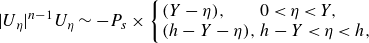 \begin{equation} |U_\eta |^{n-1} U_\eta \sim - P_s \times \left \{ \begin{array}{ll} (Y-\eta ), & 0\lt \eta \lt Y, \cr (h-Y - \eta ), & h-Y\lt \eta \lt h, \end{array}\right . \end{equation}
with
 \begin{equation} Y = \frac {h}{2} - \frac {\textit{Bi}}{|P_s|} . \end{equation}
Over the region $Y\lt \eta \lt h-Y$
, the shear stress
$Y\lt \eta \lt h-Y$
, the shear stress $\tau _{_{SN}}$
becomes less than
$\tau _{_{SN}}$
becomes less than $\textit{Bi}$
and it appears that the total stress must fall below the yield threshold. However, for
$\textit{Bi}$
and it appears that the total stress must fall below the yield threshold. However, for $\eta \to Y$
from below, or
$\eta \to Y$
from below, or $\eta \to h-Y$
from above,
$\eta \to h-Y$
from above, $U_\eta$
becomes small, and it is no longer acceptable to assume that
$U_\eta$
becomes small, and it is no longer acceptable to assume that ${\tau _{_{SN}}}\gg {\tau _{_{\textit{SS}}}}$
. Indeed, it is possible to satisfy the constitutive law by taking the stress components to be of the same order, with
${\tau _{_{SN}}}\gg {\tau _{_{\textit{SS}}}}$
. Indeed, it is possible to satisfy the constitutive law by taking the stress components to be of the same order, with
 \begin{equation} U\sim U_p(s) + U_1(s,\eta ) + \ldots, \end{equation}
as long as $U_p\gg U_1$
and
$U_p\gg U_1$
and $U_{1\eta }=O(U_{px})$
. In this setting the constitutive law corresponds to the perfectly plastic relation
$U_{1\eta }=O(U_{px})$
. In this setting the constitutive law corresponds to the perfectly plastic relation
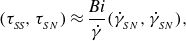 \begin{equation} ({\tau _{_{\textit{SS}}}},{\tau _{_{SN}}}) \approx \frac {\textit{Bi}}{{\dot \gamma }} ({\dot \gamma _{_{SN}}}, {\dot \gamma _{_{SN}}}), \end{equation}
and we can adopt this alternative strategy for solving the constitutive relation over $Y\lt \eta\lt h$
. Because
$Y\lt \eta\lt h$
. Because $U_{\eta }$
is relatively small here, this region is often called a ‘pseudo-plug’ in the viscoplastic fluids literature (Walton & Bittleston Reference Walton and Bittleston1991), and it is a mistake to view
$U_{\eta }$
is relatively small here, this region is often called a ‘pseudo-plug’ in the viscoplastic fluids literature (Walton & Bittleston Reference Walton and Bittleston1991), and it is a mistake to view $\eta =Y$
and
$\eta =Y$
and $\eta =h-Y$
as genuine yield surfaces (this is the core of the fallacy of the lubrication paradox). Indeed, it typically turns out that the plug-like flow speed,
$\eta =h-Y$
as genuine yield surfaces (this is the core of the fallacy of the lubrication paradox). Indeed, it typically turns out that the plug-like flow speed, $U\sim U_p(s)$
, depends on position along the gap and cannot be rigid.
$U\sim U_p(s)$
, depends on position along the gap and cannot be rigid.
In other words, the sections $0\lt \eta \lt Y$
and
$0\lt \eta \lt Y$
and $h-Y\lt \eta \lt h$
are relatively strongly sheared, viscoplastic flow regions. The central section
$h-Y\lt \eta \lt h$
are relatively strongly sheared, viscoplastic flow regions. The central section $Y\lt \eta \lt h-Y$
, however, deforms plastically and is simply the thin-gap relative of a nearly plastic zone (§ 3.4). The flow profile is
$Y\lt \eta \lt h-Y$
, however, deforms plastically and is simply the thin-gap relative of a nearly plastic zone (§ 3.4). The flow profile is
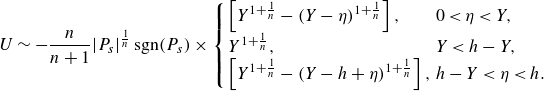 \begin{equation} U \sim - \frac {n}{n+1}|P_s|^{\frac 1n}\; \textrm {sgn}(P_s) \times \left \{ \begin{array}{ll} \left[Y^{1+\frac 1n}-(Y-\eta )^{1+\frac 1n} \right], & 0\lt \eta \lt Y, \cr Y^{1+\frac 1n}, & Y \lt h-Y,\cr \left[Y^{1+\frac 1n}-(Y-h+\eta )^{1+\frac 1n} \right], & h-Y\lt \eta \lt h. \end{array} \right . \end{equation}
Note that, in a full asymptotic analysis, narrow transition regions surrounding the fake yield surfaces $\eta =Y$
and
$\eta =Y$
and $\eta =h-Y$
are required to smooth out the join between the pseudo-plug and sheared regions (Walton & Bittleston Reference Walton and Bittleston1991; Putz et al. Reference Putz, Burghelea, Frigaard and Martinez2008; Muravleva Reference Muravleva2015). These layers, however, have no impact on the leading-order solutions elsewhere and therefore need no explicit consideration.
$\eta =h-Y$
are required to smooth out the join between the pseudo-plug and sheared regions (Walton & Bittleston Reference Walton and Bittleston1991; Putz et al. Reference Putz, Burghelea, Frigaard and Martinez2008; Muravleva Reference Muravleva2015). These layers, however, have no impact on the leading-order solutions elsewhere and therefore need no explicit consideration.
The pressure gradient, or equivalently $Y$
, must be determined by considering mass conservation across the gap
$Y$
, must be determined by considering mass conservation across the gap
 \begin{equation} \frac {\partial }{\partial {s}} \int _0^h U \; \textrm {d}\eta = - \frac {\partial }{\partial {s}}\left [\frac {n(h+2nh-2nY)}{(2n+1)(n+1)} |P_s|^{\frac 1n}Y^{1+\frac 1n} \; \textrm {sgn}(P_s) \right ] = V(s,h) - V(s,0). \end{equation}
After an integral in $s$
, and the addition of an unknown flux constant, this furnishes an algebraic equation to solve for either
$s$
, and the addition of an unknown flux constant, this furnishes an algebraic equation to solve for either $P_s$
or
$P_s$
or $Y$
. Last, with the solution for the pressure gradient in hand, we determine the unknown flux constant by integrating
$Y$
. Last, with the solution for the pressure gradient in hand, we determine the unknown flux constant by integrating $P_s$
over the lubrication layer and applying the boundary conditions on
$P_s$
over the lubrication layer and applying the boundary conditions on $P$
at the ends.
$P$
at the ends.
C.2.1. Narrow annulus
In the Bingham squeeze-flow example presented in § 5.2, $s$
is equivalent to the angle turned around the annular gap, and we have the correspondences
$s$
is equivalent to the angle turned around the annular gap, and we have the correspondences
 \begin{equation} s \equiv \phi, \quad \eta \equiv \ell -r, \quad h \equiv \unicode{x1D6E5} = \ell -1, \quad V(s,h)\equiv 0, \quad V(s,0)\equiv -\cos \phi; \end{equation}
( $n=1$
, and the inner wall of the annulus moves to the right with unit speed, which prescribes this particular
$n=1$
, and the inner wall of the annulus moves to the right with unit speed, which prescribes this particular $V(s,0)$
, and demands that
$V(s,0)$
, and demands that $U(s,0)\approx 0$
because
$U(s,0)\approx 0$
because $U\gg V$
).
$U\gg V$
).
In this case, reflection symmetry about $\theta =0$
implies that the flux constant vanishes after integrating equation (C31), and we arrive at the cubic,
$\theta =0$
implies that the flux constant vanishes after integrating equation (C31), and we arrive at the cubic,
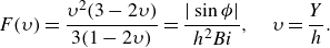 \begin{equation} F(\upsilon ) = \frac {\upsilon ^2(3-2\upsilon )}{3(1 - 2\upsilon )} = \frac {|\sin \phi |}{h^2\textit{Bi}}, \quad \upsilon = \frac {Y}{h} . \end{equation}
Note that this cubic implies that $B=h^2\textit{Bi}$
is a more natural Bingham number for the narrow-gap geometry. The pressure gradient and plug speed are given by
$B=h^2\textit{Bi}$
is a more natural Bingham number for the narrow-gap geometry. The pressure gradient and plug speed are given by
 \begin{equation} P_s = -\frac {2\textit{Bi}}{h(1-2\upsilon )} \textrm {sgn}(\sin \phi ) \quad \& \quad U_p = \frac {\upsilon ^2h\textit{Bi}}{h(1-2\upsilon )} \textrm {sgn}(\sin \phi ) . \end{equation}
The net dissipation rate is
 \begin{align} &\mathcal{E} = \int _{-\pi }^\pi \int _0^h \tau {\dot \gamma } (\ell -\eta ) \textrm {d}\eta \textrm {d} s \sim 2 \int _{-\pi }^\pi \int _0^Y \left(\frac {1}{2} h - \eta \right) (Y-\eta ) P_s^2 \textrm {d}\eta \textrm {d} s \end{align}
 \begin{align} &\qquad\quad = \frac {2\textit{Bi}}{\ell -1} \int _{-\pi }^\pi |\sin \phi | \frac {\textrm {d} s}{(1-2\upsilon )} = - \int _{-\pi }^\pi P_s \sin \phi \; \textrm {d} s, \end{align}
which equals the power input due to the translation of the inner cylinder, $\int _{-\pi }^\pi P \cos \phi \; \textrm {d} s$
(to leading order), as it must.
$\int _{-\pi }^\pi P \cos \phi \; \textrm {d} s$
(to leading order), as it must.
C.2.2. Gravity currents
For a shallow film spreading under gravity above a flat plane (figure 21), $(s,\eta )\equiv (x,y)$
and the lubrication analysis follows along a parallel path to that sketched above (Liu & Mei Reference Liu and Mei1989; Balmforth et al. Reference Balmforth, Craster, Rust and Sassi2006). Important differences are that the flow is now time-dependent, spanning the region
$(s,\eta )\equiv (x,y)$
and the lubrication analysis follows along a parallel path to that sketched above (Liu & Mei Reference Liu and Mei1989; Balmforth et al. Reference Balmforth, Craster, Rust and Sassi2006). Important differences are that the flow is now time-dependent, spanning the region $0\lt y\lt h(x,t)$
, and gravity is included, which modifies the last of equations (3.6) by adding a term
$0\lt y\lt h(x,t)$
, and gravity is included, which modifies the last of equations (3.6) by adding a term $-1$
to the right-hand side (given that the stress scale is
$-1$
to the right-hand side (given that the stress scale is $\rho g \mathcal{H}$
). In the shallow limit, and for stress-free conditions along the top surface
$\rho g \mathcal{H}$
). In the shallow limit, and for stress-free conditions along the top surface $y=h(x,t)$
, we then find
$y=h(x,t)$
, we then find $p \sim h-y$
and
$p \sim h-y$
and ${\tau _{_{SN}}}\sim -h_x (h-\eta )$
(instead of
${\tau _{_{SN}}}\sim -h_x (h-\eta )$
(instead of $p=P(x,t)$
and (C25)). The velocity profile (assuming no-slip at
$p=P(x,t)$
and (C25)). The velocity profile (assuming no-slip at $y=0$
) becomes,
$y=0$
) becomes,
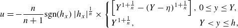 \begin{equation} u = - \frac {n}{n+1}\textrm {sgn}(h_x) \left | h_x\right |^{\frac 1n} \times \left \{ \begin{array}{ll} \left[Y^{1+\frac 1n}-(Y-\eta)^{1+\frac 1n} \right], & 0 \leq y \leq Y, \\ Y^{1+\frac 1n}, & Y \lt y \leq h, \end{array}\right . \end{equation}
where
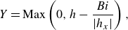 \begin{equation} Y = \textrm {Max}\left (0,h - \frac {\textit{Bi}}{ |h_x|}\right ), \end{equation}
is a fake yield surface that divides a fully shear region below from an overlying pseudo-plug; see figure 21(a).
Last, mass conservation across the gap, along with the kinematic condition $h_t + U(x,h,t) h_x = V(x,h,t)$
, furnishes the evolution equation
$h_t + U(x,h,t) h_x = V(x,h,t)$
, furnishes the evolution equation
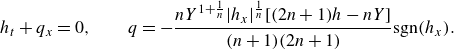 \begin{equation} h_t + q_x = 0, \qquad q = - \frac {nY^{1+\frac 1n} |h_x|^{\frac 1n}[(2n+1)h-nY]}{(n+1)(2n+1)} \textrm {sgn}(h_x) . \end{equation}
If $Y\to 0$
, the pseudo-plug expands to fill the entire fluid layer, bringing flow to rest. Given
$Y\to 0$
, the pseudo-plug expands to fill the entire fluid layer, bringing flow to rest. Given $h_x\lt 0$
, this furnishes the condition
$h_x\lt 0$
, this furnishes the condition
 \begin{equation} hh_x \approx -\textit{Bi}, \end{equation}
which leads to the profile quoted in (6.3). The convergence to this final state can be captured by setting
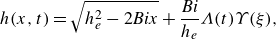 \begin{equation} h(x,t) = \sqrt {h_e^2-2\textit{Bi} x} + \frac {\textit{Bi}}{h_e}\Lambda (t) \Upsilon (\xi ), \end{equation}
where $h_e$
denotes the final maximum depth
$h_e$
denotes the final maximum depth
 \begin{equation} \xi = \frac {x}{X(t)}, \qquad X(t) = \frac {h_e^2}{2\textit{Bi}} - \Lambda (t), \end{equation}
and $\Lambda \ll 1$
(at least in the situation in which the entire fluid layer yields). Plugging these relations into the definition of
$\Lambda \ll 1$
(at least in the situation in which the entire fluid layer yields). Plugging these relations into the definition of $Y$
and the evolution equation leads to
$Y$
and the evolution equation leads to
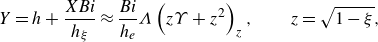 \begin{equation} Y = h + \frac {X\textit{Bi}}{h_\xi } \approx \frac {\textit{Bi}}{h_e}\Lambda \left( z\Upsilon+z^2 \right)_z, \qquad z = \sqrt {1-\xi }, \end{equation}
and
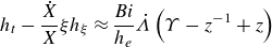 \begin{align} &\quad\qquad h_t - \frac {\dot {X}}{X}\xi h_\xi \approx \frac {\textit{Bi}}{h_e} \dot {\Lambda } \left (\Upsilon - z^{-1} + z \right ) \end{align}
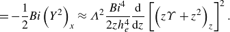 \begin{align} & = - \frac {1}{2} \textit{Bi} \left ( Y^2 \right )_x \approx \Lambda ^2 \frac {\textit{Bi}^4}{2z h_e^4} \frac {\textrm {d}}{\textrm {d}z } \left [\left( z \Upsilon + z^2 \right)_z \right ]^2 . \end{align}
That is,
 \begin{equation} \dot {\Lambda } = - \frac {1}{3k} \textit{Bi}^2\Lambda ^{2} \qquad \& \qquad 1 - \left(z\Upsilon + z^2 \right) = \frac {1}{2} k \frac {\textrm {d}}{\textrm {d}{z} }\left [\left ( z \Upsilon + z ^2 \right )_z \right ]^2, \end{equation}
for some separation constant $k$
, and since
$k$
, and since $h_e^3 = 3\textit{Bi}$
when
$h_e^3 = 3\textit{Bi}$
when $h_\infty \to 0$
. The solution therefore converges to the final state as
$h_\infty \to 0$
. The solution therefore converges to the final state as $\Lambda \sim (\textit{Bi}^2 t / 3k)^{-1}$
. The analysis of the ordinary differential equation for
$\Lambda \sim (\textit{Bi}^2 t / 3k)^{-1}$
. The analysis of the ordinary differential equation for $\Upsilon(z)$
further demands that
$\Upsilon(z)$
further demands that $k\approx 0.0866$
, which corresponds to ensuring that the solution remains regular at both
$k\approx 0.0866$
, which corresponds to ensuring that the solution remains regular at both $z =0$
and
$z =0$
and $z =1$
(where
$z =1$
(where $\Upsilon =0$
and
$\Upsilon =0$
and $\Upsilon =1$
, respectively; see Matson & Hogg (Reference Matson and Hogg2007)).
$\Upsilon =1$
, respectively; see Matson & Hogg (Reference Matson and Hogg2007)).
C.3. Lubrication analysis for annular squeeze flow with plugs
The squeeze-flow problem in § 5.2 has an order-one transverse (radial) velocity $V$
. For a thin gap, of thickness
$V$
. For a thin gap, of thickness ${\epsilon }\ll 1$
, the velocity along the gap must therefore be
${\epsilon }\ll 1$
, the velocity along the gap must therefore be $O({\epsilon }^{-1})$
, and so the shear is
$O({\epsilon }^{-1})$
, and so the shear is $U_\eta =O({\epsilon }^{-2})$
. The lubrication analysis of § C.2 therefore requires some rescaling in order to fully appreciate the asymptotics at work. In particular, it is helpful to introduce the scaled variables
$U_\eta =O({\epsilon }^{-2})$
. The lubrication analysis of § C.2 therefore requires some rescaling in order to fully appreciate the asymptotics at work. In particular, it is helpful to introduce the scaled variables
 \begin{equation} \eta = {\epsilon } \zeta, \quad ({\tau _{_{\textit{SS}}}},{\tau _{_{SN}}}) = {\epsilon }^{-2} ({\mathcal{T}_{_{\textit{SS}}}},{\mathcal{T}_{_{SN}}}), \quad p = {\epsilon }^{-3} \Pi, \quad \textit{Bi} = {\epsilon }^{-2} B, \quad U = {\epsilon }^{-1} u ;\end{equation}
(recycling some notation for the last variable). Noting that $\kappa =1$
, the curvilinear force-balance equations in (3.6) can then be written as
$\kappa =1$
, the curvilinear force-balance equations in (3.6) can then be written as
 \begin{equation} \Pi _s = (1-{\epsilon }\zeta )\frac {\partial }{\partial {\zeta }} {\mathcal{T}_{_{SN}}} + {\epsilon } \frac {\partial }{\partial {s}}{\mathcal{T}_{_{\textit{SS}}}} - 2{\epsilon } {\mathcal{T}_{_{SN}}}, \quad \Pi _\zeta + {\epsilon } \frac {\partial }{\partial {\zeta }}{\mathcal{T}_{_{\textit{SS}}}} = O({\epsilon }^2). \end{equation}
The leading-order terms here present the usual lubrication balances. We further have the mass conservation relation
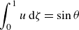 \begin{equation} \int _0^1 u \; \textrm {d} \zeta = \sin \theta \end{equation}
and (Bingham) constitutive law
 \begin{equation} \begin{pmatrix} {\mathcal{T}_{_{\textit{SS}}}} \cr {\mathcal{T}_{_{SN}}} \end{pmatrix} \sim \left ( 1 + \frac {B}{\Gamma }\right ) \begin{pmatrix} 2{\epsilon } u_s \cr u_\zeta +{\epsilon } u \end{pmatrix},\quad \Gamma = \sqrt {(u_\zeta +{\epsilon } u)^2 + 4 {\epsilon }^2 u_s^2}, \end{equation}
for ${\mathcal{T}_{_{\textit{SS}}}}^2+{\mathcal{T}_{_{SN}}}^2 \gt B^2$
(to
${\mathcal{T}_{_{\textit{SS}}}}^2+{\mathcal{T}_{_{SN}}}^2 \gt B^2$
(to $O({\epsilon }^2)$
).
$O({\epsilon }^2)$
).
Focusing on the upper part of the annulus ( $0\lt \theta \lt \pi$
), the scale of the small true plug that appears near
$0\lt \theta \lt \pi$
), the scale of the small true plug that appears near $s=\theta = (1/2)\pi$
is relatively small, though not as small as the gap itself. Consequently, we further set
$s=\theta = (1/2)\pi$
is relatively small, though not as small as the gap itself. Consequently, we further set
 \begin{equation} s = \frac {1}{2} \pi + \delta \xi, \end{equation}
where ${\epsilon } \ll \delta \ll 1$
. The first relation in (C48) becomes
${\epsilon } \ll \delta \ll 1$
. The first relation in (C48) becomes
 \begin{equation} \frac {1}{\delta } \Pi _\xi = \frac {\partial }{\partial {\zeta }} {\mathcal{T}_{_{SN}}} + \frac {{\epsilon }}{\delta } \frac {\partial }{\partial {\xi }}{\mathcal{T}_{_{\textit{SS}}}} + O({\epsilon }); \end{equation}
(the second is unchanged). The constitutive law implies that $\mathcal{T}_{_{\textit{SS}}}$
is
$\mathcal{T}_{_{\textit{SS}}}$
is $O({\epsilon }\delta ^{-1})\ll 1$
smaller than
$O({\epsilon }\delta ^{-1})\ll 1$
smaller than $\mathcal{T}_{_{SN}}$
where the fluid is yielded, and the mass conservation constraint becomes
$\mathcal{T}_{_{SN}}$
where the fluid is yielded, and the mass conservation constraint becomes
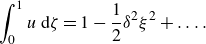 \begin{equation} \int _0^1 u \; \textrm {d} \zeta = 1 - \frac {1}{2}\delta ^2\xi ^2 + \ldots .\end{equation}
To solve the problem, we therefore introduce the sequences
 \begin{equation} \Pi = \delta \Pi _0 + {\epsilon } \Pi _1 +\ldots, \!\!\!\!\quad {\mathcal{T}_{_{SN}}} = \mathcal{T}_0 + \frac {{\epsilon }}{\delta } \mathcal{T}_1+\ldots, \!\!\!\!\quad u = u_0 + \frac {{\epsilon }}{\delta } u_1 +\ldots, \!\!\!\!\quad {\mathcal{T}_{_{\textit{SS}}}} = \Sigma _0 + \ldots. \end{equation}
The problem is also now symmetrical about $\zeta = 1/2$
, leading us to consider the inner half of the annulus with
$\zeta = 1/2$
, leading us to consider the inner half of the annulus with $0\lt \zeta \lt 1/2$
.
$0\lt \zeta \lt 1/2$
.
At leading order, we find that
 \begin{equation} \Pi _{0\xi } = \mathcal{T}_{0\zeta }, \quad \Pi _{0\zeta } = 0, \quad \mathcal{T}_0 = u_{0\zeta } + B, \end{equation}
with solution
 \begin{equation} \mathcal{T}_0 = - \left(\frac {1}{2}-\zeta \right)\Pi _{0\xi },\quad u_0 = - \frac {1}{2} \zeta (2Y_0-\zeta ) \Pi _{0\xi }, \quad Y_0 = \frac {1}{2} - \frac {B}{|\Pi _{0\xi }|}, \end{equation}
applying in $0\lt \zeta \lt Y_0$
(where
$0\lt \zeta \lt Y_0$
(where $\Pi _{0\xi }\lt 0$
), and
$\Pi _{0\xi }\lt 0$
), and $u_{0\zeta }=0$
in
$u_{0\zeta }=0$
in $Y_0\lt \zeta \lt 1/2$
. This reproduces the solution in § C.2 except that the leading-order mass conservation constraint boils down to
$Y_0\lt \zeta \lt 1/2$
. This reproduces the solution in § C.2 except that the leading-order mass conservation constraint boils down to
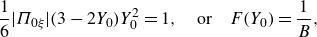 \begin{equation} \frac {1}{6} |\Pi _{0\xi }| (3-2Y_0)Y_0^2 = 1, \quad \textrm {or} \quad F(Y_0)= \frac {1}{B}, \end{equation}
and demands that $P_{0\xi }$
,
$P_{0\xi }$
, $Y_0$
and
$Y_0$
and $u_{p0}=- (1/2)\Pi _{0\xi }Y_0^2$
are all constant.
$u_{p0}=- (1/2)\Pi _{0\xi }Y_0^2$
are all constant.
At $O({\epsilon }\delta ^{-1})$
we arrive at the equations
$O({\epsilon }\delta ^{-1})$
we arrive at the equations
 \begin{equation} \Pi _{1\xi } = \mathcal{T}_{1\zeta } + \Sigma _{0\xi }, \quad (\Pi _1 + \Sigma _0)_\zeta = 0 . \end{equation}
But $\Sigma _0=0$
and
$\Sigma _0=0$
and $\mathcal{T}_1=u_{1\zeta }$
over the yielded region, and so for
$\mathcal{T}_1=u_{1\zeta }$
over the yielded region, and so for $0\lt \zeta \lt Y_0$
we find
$0\lt \zeta \lt Y_0$
we find
 \begin{equation} \Pi _1=\Pi _1(\xi ),\quad \mathcal{T}_1 = T_1 + \zeta \Pi _{1\xi }\quad \& \quad u_1 = \zeta T_1 + \frac {1}{2} \zeta ^2\Pi _{1\xi } . \end{equation}
Over the plug, the solution is less clear as $\Sigma _0$
need not vanish, and (C58) do not provide sufficient conditions to determine all of
$\Sigma _0$
need not vanish, and (C58) do not provide sufficient conditions to determine all of $\Pi _1$
,
$\Pi _1$
, $\mathcal{T}_1$
and
$\mathcal{T}_1$
and $\Sigma _0$
, which corresponds to the usual indeterminacy below the yield stress. Setting that complication to one side, we observe that the corrections to the leading-order solution imply shifts to the yield surface position and plug velocity from
$\Sigma _0$
, which corresponds to the usual indeterminacy below the yield stress. Setting that complication to one side, we observe that the corrections to the leading-order solution imply shifts to the yield surface position and plug velocity from
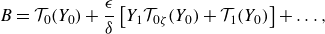 \begin{equation} B=\mathcal{T}_0(Y_0) + \frac {{\epsilon }}{\delta }\left[Y_1\mathcal{T}_{0\zeta }(Y_0) + \mathcal{T}_1(Y_0) \right]+\ldots, \end{equation}
and
 \begin{equation} u_{p0}+\frac {{\epsilon }}{\delta }u_{p1}+\ldots = u_{0}(Y_0) + \frac {{\epsilon }}{\delta } \left[Y_1u_{0\zeta }(Y_0) + u_1(Y_0) \right]+\ldots .\end{equation}
That is,
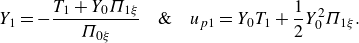 \begin{equation} Y_1 = -\frac {T_1+Y_0\Pi _{1\xi }}{\Pi _{0\xi }} \quad \& \quad u_{p1} = Y_0 T_1 + \frac {1}{2} Y_0^2 \Pi _{1\xi }. \end{equation}
The last of these implies a constraint, as $u_{1p}$
should be constant.
$u_{1p}$
should be constant.
With these corrections in hand, mass conservation now demands that
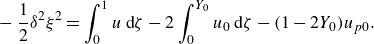 \begin{equation} -\frac {1}{2} \delta ^2 \xi ^2 = \int _0^1 u \; \textrm {d}\zeta - 2\int _0^{Y_0} u_0 \; \textrm {d}\zeta - (1-2Y_0) u_{p0}. \end{equation}
The right-hand side of this expression of $O({\epsilon }\delta ^{-1})$
. To match the
$O({\epsilon }\delta ^{-1})$
. To match the $O(\delta ^2)$
terms on the left, we must therefore select
$O(\delta ^2)$
terms on the left, we must therefore select $\delta ={\epsilon }^{\frac 13}$
. We then find
$\delta ={\epsilon }^{\frac 13}$
. We then find
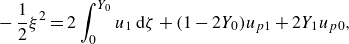 \begin{equation} -\frac {1}{2}\xi ^2 = 2\int _0^{Y_0} u_1 \; \textrm {d}\zeta + (1-2Y_0) u_{p1} + 2Y_1 u_{p0}, \end{equation}
or
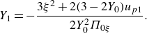 \begin{equation} Y_1 = -\frac {3\xi ^2+2(3-2Y_0)u_{p1}}{2Y_0^2\Pi _{0\xi }} . \end{equation}
At the edge of the plug, $\xi =\xi _*$
, the solution must smoothly join on to that for the pseudo-plug, given that the shape of the yield surface varies over a much shorter scale (
$\xi =\xi _*$
, the solution must smoothly join on to that for the pseudo-plug, given that the shape of the yield surface varies over a much shorter scale ( $O({\epsilon })$
) than the plug width. The leading-order pseudo-plug solution is given by
$O({\epsilon })$
) than the plug width. The leading-order pseudo-plug solution is given by
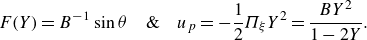 \begin{equation} F(Y)=B^{-1}\sin \theta \quad \& \quad u_p=-\frac {1}{2}\Pi _\xi Y^2 = \frac {B Y^2}{1-2Y} . \end{equation}
Corrections to these expressions are not expected at $O(\epsilon \delta ^{-1}\equiv {\epsilon }^{\frac 23})$
in the bulk of the pseudo-plug, and so the match demands that
$O(\epsilon \delta ^{-1}\equiv {\epsilon }^{\frac 23})$
in the bulk of the pseudo-plug, and so the match demands that
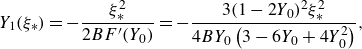 \begin{equation} Y_1(\xi _*) = - \frac {\xi _*^2}{2BF'(Y_0)} =-\frac {3(1-2Y_0)^2\xi _*^2}{4BY_0 \left(3-6Y_0+4Y_0^2 \right)}, \end{equation}
and
 \begin{equation} u_{p1} = \frac {2Y_0B(1-Y_0)}{(1-2Y_0)^2} Y_1(\xi _*) = - \frac {3(1-Y_0)\xi _*^2}{2 \left(3-4Y_0+4Y_0^2 \right)}, \end{equation}
which are consistent with (C65). This must be true because, at this stage, the solution simply corresponds to an expansion of that for the pseudo-plug for $\theta =\frac {1}{2}\pi +\delta \xi _*$
, given that the only new addition to the problem, the extensional stress
$\theta =\frac {1}{2}\pi +\delta \xi _*$
, given that the only new addition to the problem, the extensional stress $\Sigma _0$
, has not yet made a decisive appearance.
$\Sigma _0$
, has not yet made a decisive appearance.
Last, we must consider the force balance on the plug: (C58) imply
 \begin{equation} \Pi _1(\xi, \zeta ) = \Pi _1(\xi, Y_0) - \Sigma _0(\xi, \zeta ) \quad \& \quad \int _{Y_0}^{\frac 12} \left[\Pi _1(\xi, Y_0)-2\Sigma _0 \right]_\xi \textrm {d}\zeta = - \mathcal{T}_1(\xi, Y_0), \end{equation}
since $\Sigma _0(\xi, Y_0)=0$
and
$\Sigma _0(\xi, Y_0)=0$
and $\mathcal{T}_1(\xi, ({1}/{2})=0$
. That is,
$\mathcal{T}_1(\xi, ({1}/{2})=0$
. That is,
 \begin{equation} \frac {\partial }{\partial {\xi }} \int _{Y_0}^{\frac 12} \Sigma _0 \textrm {d}\zeta = \frac {1}{2} T_1 + \frac {1}{4} \Pi _{1\xi }(\xi, Y_0) \frac {2u_{p1}\left(3-6Y_0+4Y_0^2 \right)}{4Y_0^3} + \frac {3(1-Y_0)\xi ^2}{4Y_0^3} . \end{equation}
Symmetry about $\xi =0$
(
$\xi =0$
( $\phi = ({1}/{2})\pi$
) then indicates that
$\phi = ({1}/{2})\pi$
) then indicates that
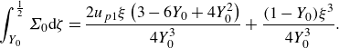 \begin{equation} \int _{Y_0}^{\frac 12} \Sigma _0 \textrm {d}\zeta = \frac {2u_{p1}\xi \left(3-6Y_0+4Y_0^2 \right)}{4Y_0^3} + \frac {(1-Y_0)\xi ^3}{4Y_0^3} . \end{equation}
But where the plug breaks, the extensional stress $\Sigma _0$
must match with that for the pseudo-plug, which is
$\Sigma _0$
must match with that for the pseudo-plug, which is
 \begin{equation} \Sigma _0 = \pm \sqrt {B^2 - \mathcal{T}_0^2} = \pm \sqrt {B^2 - \left(\frac {1}{2}-\zeta \right)^2\Pi _{0\xi }^2}. \end{equation}
Evaluating the integral at $\xi =\xi _*$
as
$\xi =\xi _*$
as $- (1/4) \pi B( (1/2)-Y_0)$
now gives
$- (1/4) \pi B( (1/2)-Y_0)$
now gives
 \begin{equation} -\left(\frac {1}{2}-Y_0 \right)\pi B Y_0^3 = 2u_{p1}\xi _*(3-6Y_0+4Y_0^2) + (1-Y_0)\xi _*^3 = -2(1-Y_0)\xi _*^3 . \end{equation}
That is,
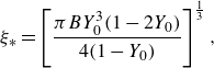 \begin{equation} \xi _* = \left [ \frac {\pi B Y_0^3(1-2Y_0)}{4(1-Y_0)}\right ]^{\frac 13}, \end{equation}
which is plotted as a function of $B$
in figure 26 along with plug sizes measured from numerical solutions. The plug length has the interesting feature that it is a non-monotonic function of Bingham number (which is already evident from the numerical solutions in figure 11).
$B$
in figure 26 along with plug sizes measured from numerical solutions. The plug length has the interesting feature that it is a non-monotonic function of Bingham number (which is already evident from the numerical solutions in figure 11).

Figure 26. Plug lengths $\xi _*\equiv ( ({1}/{2})\pi -\phi _*)/\unicode{x1D6E5} ^{1/3}$
plotted against rescaled Bingham number,
$\xi _*\equiv ( ({1}/{2})\pi -\phi _*)/\unicode{x1D6E5} ^{1/3}$
plotted against rescaled Bingham number, $B=\unicode{x1D6E5} ^2 \textit{Bi}$
. The solid line shows (C74) and the stars indicate measurements from numerical solutions with
$B=\unicode{x1D6E5} ^2 \textit{Bi}$
. The solid line shows (C74) and the stars indicate measurements from numerical solutions with $\unicode{x1D6E5} = {1}/{20}$
; the triangles show the measurements from the solutions shown in figure 11 with
$\unicode{x1D6E5} = {1}/{20}$
; the triangles show the measurements from the solutions shown in figure 11 with $\unicode{x1D6E5} = 1/5$
.
$\unicode{x1D6E5} = 1/5$
.


 Open access