


Introduction
In recent years, scholars have discovered remarkable inequalities in who gets represented in electoral democracies around the world. In the United States, a number of studies find that elected representatives appear to respond almost exclusively to the preferences of the very affluent when they pursue legislation (e.g., Flavin Reference Flavin2014; Bartels Reference Bartels2008; Gilens Reference Gilens2012; Jacobs & Page Reference Jacobs and Page2005). Other US studies raise questions about these findings and the extent of the inequality (e.g., Enns Reference Enns2015; Branham et al. Reference Branham, Soroka and Wlezien2017; Brunner et al. Reference Brunner, Ross and Washington2013; Bhatti & Erikson Reference Bhatti, Erikson, Enns and Wlezien2001). Yet, outside the United States, the growing number of studies all seem to find similarly unequal representation (e.g., Bernauer et al. Reference Bernauer, Giger and Rosset2015; Giger et al. Reference Giger, Rosset and Bernauer2012; Lupu & Warner Reference Lupu, Warner, Joignant, Morales and Fuentes2017; Peters & Ensink Reference Peters and Ensink2015; Schakel et al. Reference Schakel, Burgoon and Hakhverdian2020; Schakel & Hakhverdian Reference Schakel and Hakhverdian2018; Rosset et al. Reference Rosset, Giger and Bernauer2013; Rosset & Stecker Reference Rosset and Stecker2019; Rosset Reference Rosset2016; Lesschaeve Reference Lesschaeve2017; Donnelly & Lefkofridi Reference Donnelly and Lefkofridi2014).Footnote 1
In the most comprehensive study to date, Lupu and Warner (Reference Lupu and WarnerForthcoming) find that more affluent citizens are on average better represented by their elected officials than are poorer citizens. Digging deeper into specific cases, they find that this affluence bias exists on socioeconomic issues – and that a pro‐poor bias exists on social or cultural issues (see also Gilens Reference Gilens2012; Lesschaeve Reference Lesschaeve2017; Rosset & Stecker Reference Rosset and Stecker2019; Bartels Reference Bartels2016). But their comparative dataset focuses on left–right positions that appear to capture socioeconomic policy preferences.
We use their dataset to study what might be driving unequal representation around the world. Why is representation more unequal in some countries and in some years than others? To date, most scholarship on unequal representation has focused on documenting its existence and variation. Only a handful of studies examine the question of why representation tends to be unequal (Bernauer et al. Reference Bernauer, Giger and Rosset2015; Rosset Reference Rosset2016; Guntermann et al. Reference Guntermann, Dassonneville and Miller2020; Flavin Reference Flavin2014; Bartels Reference Bartels2008; Gilens Reference Gilens2012). And even these largely test just one or two potential explanations – such as campaign finance regulations or electoral disproportionality – in isolation.
Many plausible alternative explanations also exist, including income inequality, government partisanship, trade union strength and corruption, to name a few. In this paper, we leverage variation across time and space to adjudicate among these plausible explanations for what drives unequal representation. That is, in order to understand why representation is unequal on average, we ask why it is more unequal in some times and places than in others. We focus on five groups of possible explanations: those focusing on economic conditions, political institutions, governance, interest groups and political behaviour.
The list of plausible explanations is long, and unequal representation is undoubtedly multi‐causal. There is also little in the way of theory about how to model these explanations or the interdependent relationships among the explanatory variables. Our aim is descriptive and not causal.Footnote 2 We want to know which of the many possible explanations for unequal representation seem to matter empirically so that scholars can begin to develop more parsimonious theories that can be tested. For this reason, we use machine learning rather than only vanilla linear regression analysis to evaluate which variables better explain the variation in the data (see Molina & Garip Reference Molina and Garip2019; Grimmer Reference Grimmer2015).
Using the global sample, we find that variables relating to economic conditions and governance are the most important for predicting affluence bias in representation. We find little support overall for hypotheses that affluence bias might be due to factors related to political institutions, interest groups or political behaviour, such as turnout or compulsory voting. Further, we find that these variables account not only for global patterns in unequal representation but also, largely, differences among the wealthy democracies of Western Europe. Among this subset, the same basic groups of variables account for much of the variation in unequal representation, though the precise order of variable importance shifts somewhat: economic development becomes substantially less important, while campaign finance and party institutionalization become more important.
Explaining unequal representation
Canonical theories typically divide the representative process into two stages: first, congruence or opinion representation – the process of generating a body of representatives that reflects the preferences of the electorate – and then, responsiveness – the process by which these representatives generate policies that reflect citizens' preferences (Miller & Stokes Reference Miller and Stokes1963; Achen Reference Achen1978). Whereas recent empirical research on unequal representation in the United States has focused on responsiveness (e.g., Bartels Reference Bartels2008; Gilens Reference Gilens2012), comparative work has tended to focus on congruence (e.g., Bernauer et al. Reference Bernauer, Giger and Rosset2015; Giger et al. Reference Giger, Rosset and Bernauer2012; Schakel & Hakhverdian Reference Schakel and Hakhverdian2018; Lupu & Warner Reference Lupu and WarnerForthcoming). We build on this comparative work, asking why elected representatives around the world seem to be more congruent with their more affluent constituents.
One group of explanations suggests that economic conditions may affect representation. Economic development may be associated with higher levels of education, greater opportunities for class‐based mobilization and declining opportunities for clientelism – all of which might increase the policy demands of the poor (Luna & Zechmeister Reference Luna and Zechmeister2005). Conversely, where economic resources are distributed unequally, the rich may be able to exert more disproportionate influence on policymakers (Rosset et al. Reference Rosset, Giger and Bernauer2013; Erikson Reference Erikson2015). Globalization – that is, a country's dependence on foreign trade or capital – may constrain the policy space such that elected representatives may be forced to take positions preferred by international economic elites (Andrews Reference Andrews1994; Kurzer Reference Kurzer1991; Cerny Reference Cerny1999), which will presumably also be close to those of domestic elites.
A second approach suggests that domestic political institutions matter. Electoral systems with proportional representation are thought to promote more mass–elite congruence than majoritarian systems (e.g., McDonald & Budge Reference McDonald and Budge2005; Huber & Powell Reference Huber and Powell1994; Powell Reference Powell2009), although some studies challenge that finding (e.g., Blais & Bodet Reference Blais and Bodet2006; Golder & Lloyd Reference Golder and Lloyd2014; Ferland Reference Ferland2016; Lupu et al. Reference Lupu, Selios and Warner2017). The logic is that proportional systems ensure that a larger swath of the electorate is represented in the legislature, which might also reduce biases toward the rich (see Bernauer et al. Reference Bernauer, Giger and Rosset2015). Representation may also be more equal in contexts where democratic governance and party systems are more consolidated. In these contexts, where party labels may be more informative (Lupu Reference Lupu2016), voters might be better able to select candidates who represent their preferences. Contexts with more robust political parties may also provide institutional vehicles for recruiting and supporting politicians who are less biased toward the preferences of the rich.
A third group of explanations focuses on different forms of governance. Where clientelism and corruption are rampant, representatives may have incentives to emphasize the preferences of the affluent because they fund their political machines or because poor voters are bought off (Stokes Reference Stokes2005). The ideological makeup of the legislature might also matter. Since leftist parties typically have less affluent core constituencies (Garrett Reference Garrett1998; Korpi & Palme Reference Korpi and Palme2003; Huber & Stephens Reference Huber and Stephens2001), having more leftists in office may produce less affluence bias.Footnote 3 Finally, some studies find that female representatives prioritize pro‐poor policies more than their male counterparts (Clayton et al. Reference Clayton, Josefsson, Mattes and Mozaffar2019), suggesting that legislatures with more female representatives may be less biased in favour of the rich.
Interest groups often also play a substantial role in determining who runs for and wins public office (Grossman & Helpman Reference Grossman and Helpman2001). Some interest groups favour the preferences of the rich while others emphasize the preferences of the poor, and the relative strength of these types of groups could help determine whether elected representatives better reflect one side over the other. For instance, since trade unions tend to represent the interests of the less affluent (Korpi Reference Korpi1983), contexts with stronger unions might demonstrate less affluence bias.
Scholars of US politics tend to focus on the role that interest groups and affluent citizens play through political donations (e.g., Flavin Reference Flavin2014; Bartels Reference Bartels2008; Gilens Reference Gilens2012). Since affluent voters and their allied interest groups are the source of most of the money involved in political campaigns, it seems plausible that they use their wealth to shift the selection of policymakers closer to their preferences. Although we know far less about the role of money in politics outside the United States (Scarrow Reference Scarrow2007), campaign contributions may similarly bias representation in other democracies (see Rosset Reference Rosset2016).
A final group of theories suggests that unequal representation might arise primarily through different patterns in political behaviour. For instance, the affluence bias might just be a function of poor people being less likely to vote than the rich (e.g., Schlozman et al. Reference Schlozman, Verba and Brady2012; Lijphart Reference Lijphart1997; Avery Reference Avery2015; Leighley & Nagler Reference Leighley and Nagler2013). If elected representatives are re‐election oriented, they may discount the preferences of citizens who are unlikely to turn out to vote (Guntermann et al. Reference Guntermann, Dassonneville and Miller2020). Although disproportionate turnout among the rich is less common in developing countries (Kasara & Suryanarayan Reference Kasara and Suryanarayan2015; Gallego Reference Gallego2015), it is plausible that elected representatives discount the preferences of the poor in contexts where they participate less. A related possibility is that political cleavages cross‐cut, such that political dimensions beyond affluence – such as ethnicity or region – inform political selection (Lipset Reference Lipset1960). In these cases, we might see unequal representation on the affluence dimension but more equal representation along other salient cleavage dimensions.
Scholars are only beginning to evaluate which of these competing arguments might best explain the patterns of unequal representation around the world. Studies of the United States generally conclude that the role of money in US politics is the most apt explanation for the inequalities they find (Flavin Reference Flavin2014; Bartels Reference Bartels2008; Gilens Reference Gilens2012). But their evidence is largely indirect, and they rule out only a small number of alternatives – most notably, disproportionately lower turnout by the less affluent. Comparative studies have only recently begun to study the topic, offering support for the importance of electoral institutions, turnout, and party public financing (Guntermann et al. Reference Guntermann, Dassonneville and Miller2020; Bernauer et al. Reference Bernauer, Giger and Rosset2015; Rosset Reference Rosset2016). But these, too, largely test a single explanation in isolation. We are still far from understanding why representation is unequal.
Empirical strategy
To answer this question, we use a new dataset on mass–elite ideological congruence worldwide. Lupu and Warner (Reference Lupu and WarnerForthcoming) collected every publicly available survey of national representatives or candidates in which respondents were asked to place themselves on a scale with ‘left’ and ‘right’ (or similar) anchors.Footnote 4 They then matched these elite surveys with data on mass preferences using publicly available surveys in which voting‐age adults were similarly asked to place themselves on a left–right scale.Footnote 5
The resulting dataset includes 92,000 unique legislator‐year observations matched to 3.9 million citizen‐year observations. It spans 565 country‐years across 52 countries and 33 years, the largest collection of mass and elite ideological preferences of which we are aware.Footnote 6 Although the dataset represents all of the available information, note that it comes overwhelmingly from Europe and Latin America. To avoid problems arising from small samples, we restrict our analysis to the 285 country‐years in which responses for at least 30 legislators and 30 citizens are available.
Our dependent variable is a measure of congruence, the similarity between the preferences of citizens and those of their elected representatives. We compute congruence for each country‐year using the earth mover's distance (EMD), a measure of distributional similarity that has been shown to better capture mass–elite congruence than alternative approaches (Lupu et al. Reference Lupu, Selios and Warner2017). The EMD between two distributions solves a linear optimization problem, the optimal flow of mass from one distribution to the other until they are identical. In our case, the EMD captures the distance, or similarity, between the distribution of preferences of citizens and the distribution of preferences of elected representatives. We calculate the EMD for both the bottom and top quintile of citizens in terms of affluence. Since the EMD captures the distance between each distribution of citizen preferences and legislator positions, our dependent variable is the difference between these EMDs, computed as
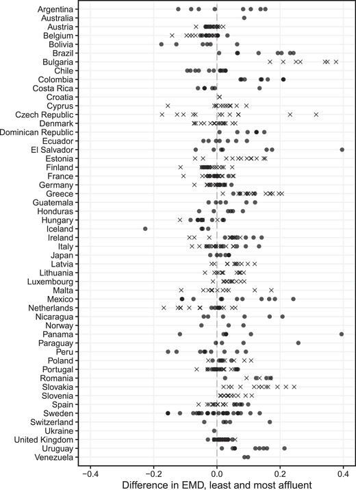
 . Larger values indicate greater affluence bias, with legislators' preferences closer to those of the rich than of the poor. Figure 1 plots the distribution of our dependent variable by country, with each point indicating a country‐year of data; crosses indicate country‐years excluded from our statistical analyses due to small sample sizes. Variation in affluence bias does not appear to be predominantly within‐ or across‐country, but rather a combination of both.

Figure 1. The distribution of affluence bias in the dataset. Each point represents the EMD between legislators and the least affluent quintile of voters, minus the EMD between legislators and the most affluent quintile of voters, for one country‐year. Positive values indicate that the poor are underrepresented relative to the rich, while negative values indicate the opposite. Dots represent observations in the statistical analyses, while crosses indicate data that are excluded because there are too few respondents in the country‐year.
To measure affluence, we develop a rank ordering of indicators, which privileges measuring wealth over household income and occupational status.Footnote 7 Where we have data on ownership of durable goods (e.g., a car or refrigerator), we use multiple correspondence analysis to generate a factored index of affluence (see Filmer & Pritchett Reference Filmer and Pritchett2001). Where these data are not available, we use household income or occupation, in that order. We then generate quintiles from the material wealth and income variables, and we recode occupational data into general categories (e.g., ‘white‐collar professional').Footnote 8
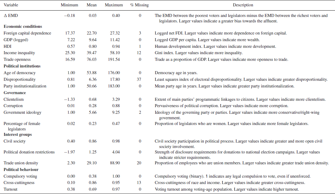
To measure our independent variables of interest, we collected data on a range of covariates to test all of the potential explanations for the affluence effect discussed above. Summary statistics and descriptions are provided in Table 1, with data sources and coding rules summarized in the online appendix.
Table 1. Summary statistics

See the text for variable sources. Note that each variable is centred and scaled prior to analysis.
The first group of variables all relate to economic conditions. To measure levels of economic development, we use GDP per capita and the United Nations' Human Development Index (HDI), a broad measure that encompasses health, education, and standard of living outcomes. Our measure of income inequality is the Gini index derived from economic household surveys and reported by the World Bank. To study the effects of globalization, we include both net foreign direct investment, as a measure of dependence on foreign capital, and trade openness.
Our second group of covariates relate to political institutions. To study the effects of electoral systems, we follow previous studies and focus on the translation of votes into seats using a Gallagher (Reference Gallagher1991) index of electoral disproportionality, as collated and updated by Gandrud (Reference Gandrud2019). For measures of how consolidated democratic governance and party systems are, we use the age of democracy calculated by Boix et al. (Reference Boix, Miller and Rosato2013) and the mean party age provided in the Database of Political Institutions (DPI; Beck et al. Reference Beck, Clarke, Groff, Keefer and Walsh2001; Cruz et al. Reference Cruz, Keefer and Scartascini2016).
The third set of covariates focuses on governance. We measure political clientelism using an index derived from expert surveys fielded by the Varieties of Democracy (V‐Dem) project (recoded from a party linkages variable). We also use V‐Dem's index of political corruption, which captures six distinct types of corruption across legislative, judicial, and executive branches of government, as well as in the public sector (Coppedge et al. Reference Coppedge, Gerring, Lindberg, Skaaning, Teorell, Altman, Bernhard, Fish, Glynn, Hicken, Knutsen, Krusell, Lührmann, Marquardt, McMann, Mechkova, Olin, Paxton, Pemstein, Pernes, Petrarca, Römer, Saxer, Seim, Sigman, Staton, Stepanova and Wilson2017). To examine government ideology, we build a measure of left–right ideology, weighted by party strength in government, for each country‐year. Our data for this variable are drawn from the Chapel Hill Expert Survey Data (CHES; Polk et al. Reference Polk, Rovny, Bakker, Edwards, Hooghe, Jolly, Koedam, Kostelka, Marks, Schumacher, Steenbergen, Vachudova and Zilovic2017; Bakker et al. Reference Bakker, Vries, Edwards, Hooghe, Jolly, Marks, Polk, Rovny, Steenbergen and Vachudova2015), adding in data from the Manifesto Project (Volkens et al. Reference Volkens, Krause, Lehmann, Matthieß, Merz, Regel and els2018) and Baker & Greene (Reference Baker and Greene2011), rescaling these sources to the same 0–10 scale as in CHES. Finally, we study the proportion of legislators who are women, which we computed by scraping the website of the Inter‐Parliamentary Union (2019), now downloadable from the Parline repository.
Our fourth group of potential explanations focuses on interest groups. Here we use a V‐Dem index of civil society participation in policymaking to measure the overall strength of civil society and International Labor Organization data on trade union density to look specifically at the role of unions. To explore the effects of campaign finance, we include V‐Dem's measure of the stringency of restrictions on political donations.
Our final group of covariates relate to political behaviour. To examine the effects of cross‐cutting cleavages, we use the measure of race–income cross‐cuttingness developed by Selway (Reference Selway2011). We also want to examine the possible effect that disproportionately lower turnout by the poor may have on unequal representation. Prior studies suggest that these inequalities in participation are lower when turnout itself is higher and when voting is compulsory (Gallego Reference Gallego2010; Persson et al. Reference Persson, Solevid and hrvall2013; Dassonneville et al. Reference Dassonneville, Hooghe and Miller2017). We derive both indicators from V‐Dem, which measures electoral turnout among the voting‐age population and a binary variable for whether citizens are required to vote, regardless of enforcement.
Modelling affluence bias
Which of these possible factors actually exert influence on the gap in representation between rich and poor? Answering this question poses methodological challenges. Representation is undoubtedly multi‐causal, but we have little in the way of theory to guide us in modelling the relationships among all of these factors, let alone their independent relationships with representation. We could simply make strong assumptions and throw all of these variables into a kitchen‐sink regression model, but this would unreasonably assert independence among the variables, assume linearity and yield conditional results that are difficult to interpret (Achen Reference Achen2005; Hindman Reference Hindman2015; Ray Reference Ray2005). It would also undoubtedly lead us to overfitting, finding relationships among variables that fit noise in our particular dataset but are unlikely to generalize beyond our sample.Footnote 9 And, like many regression analyses, making such arbitrary modelling choices would lead us to underestimate (and understate) our modelling uncertainty (Bartels Reference Bartels1997; Montgomery et al. Reference Montgomery, Hollenbach and Ward2012).
One way to resolve these issues, particularly in descriptive studies like ours, is to turn to machine learning (Molina & Garip Reference Molina and Garip2019; Athey & Imbens Reference Athey and Imbens2019; Breiman Reference Breiman2001b). Machine learning allows us to estimate models in which the parameters are algorithmically honed to provide better model fit while also incentivizing parsimony. The ensemble of machine learning algorithms we study allows for nonlinearities, interactions, nested functions and a number of other complexities that are difficult to study in the framework of linear regression. By using split samples and cross‐validation, machine learning also provides a more rigorous approach to measuring out‐of‐sample predictive power, thereby guarding against overfitting. At the same time, this approach subsumes standard linear regression, allowing us to also study the same models that could be estimated using ordinary least squares. These advantages have led more and more political scientists to use machine learning tools to study questions relating to topics as diverse as interest group politics, voting behaviour, survey research methods, legislator ideology, genocide and civil war onset (Bonica Reference Bonica2018; Cohen & Warner Reference Cohen and WarnerForthcoming; Grimmer & Stewart Reference Grimmer and Stewart2013; Hainmueller & Hazlett Reference Hainmueller and Hazlett2014; Muchlinski et al. Reference Muchlinski, Siroky, He and Kocher2016; Becker et al. Reference Becker, Fetzer and Novy2017).
We begin by imputing missing data among our independent variables.Footnote 10 Patterns of missingness in our variables vary from source to source, such that listwise deleting each observation for which we do not have data on every variable would mean losing nearly half of our sample. Overall, 11 per cent of our data are missing, so we use conditional multiple imputation to generate 11 imputation replicates, each with 10 iterations (Kropko et al. Reference Kropko, Goodrich, Gelman and Hill2014; Bodner Reference Bodner2008). Each of these replicates is then partitioned into training and test samples containing 75 and 25 per cent of the data, respectively, while preserving the marginal distributions of all variables. Training samples are used to find model parameters that produce the best predictions, while the test samples are used to measure how accurate those predictions are.
Next, we iterate through 13 machine learning algorithms using the
 package
 (Kuhn Reference Kuhn2008). The models we study include the generalized linear model, linear discriminant, nearest‐neighbour, neural network and random forest implementations, including bagged and boosted variants.Footnote 11 Together, these models include all of the major flavours of machine learning prevalent in political science. For each replicate, each model's hyperparameters (e.g., the number of layers in a neural network) are ‘tuned’ using fivefold cross‐validation with five repeats, after which the hyperparameters that provide the lowest root mean‐squared error (RMSE) are chosen (Bagnall & Cawley Reference Bagnall and Cawley2017). The model is then fitted to the training replicate using these hyperparameters and the model parameters (e.g., coefficient estimates) that minimize RMSE. These
 fitted models are then used to predict the gap in representation for observations in each of the 11 test samples.Footnote 12
We care about two quantities of interest. First, we want to know which models provide the best fit, as evident in the smallest RMSE. Second, from the best‐fitting models, we want to know which variables exert the greatest effect on the representation gap. A typical quantity in machine learning (e.g., Breiman Reference Breiman2001a; Hill & Jones Reference Hill and Jones2014), ‘variable importance’ metrics indicate the amount of information a covariate provides to the model for predicting the outcome. In essence, they tell us how much a model's predictive performance changes if each variable is removed. By default,
 rescales all variable importance measures (which differ across models) to a 0–100 scale, where zero indicates a variable provided no information to the model and 100 indicates a variable provided the most information among all covariates.Footnote 13
Which variables matter most?
All of the models we study perform reasonably well. The worst‐fitting models are two neural network implementations, each of which produces a mean RMSE of 0.086 across the 11 imputed data replicates; the best‐fitting model is a random forest with a mean RMSE of 0.074.Footnote 14 These slight differences shrink even further when we account for imputation uncertainty: all the models' standard deviation of RMSE across imputation replicates hover between 0.008 and 0.013, suggesting that most models perform as well as the others. Still, our tree‐based models generally outperform our neural networks – an unsurprising result since neural networks are more prone to overfitting, which may be a problem for our small sample. Given these findings, we interpret results from the random forest.Footnote 15
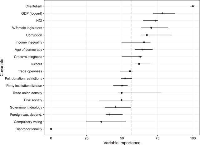
Figure 2 presents the variable importance results for the random forest. Dots indicate median importance across the imputation replicates, with lines for interquartile ranges. We do not find much evidence suggesting political institutions are important for understanding variation in affluence bias. Disproportionality ranks dead last in variable importance, and in fact is not used in any of the random forests fit to the 11 imputation replicates, suggesting that it is never informative for understanding variation in affluence bias. While age of democracy is slightly above average in importance, the last institutional variable, party system institutionalization, is of below‐average importance. Compulsory voting, foreign capital dependence, government ideology and civil society strength round out the bottom five variables alongside disproportionality. Also somewhat striking is the below‐average importance of restrictions on political donations. Taken as a whole, these results indicate that political institutions and campaign finance are far less important for determining the gap in representation between rich and poor than previously thought.

Figure 2. Variable importance. Each dot represents the mean variable importance, with lines for the interquartile range, across all imputation replications from the random forest model. Larger values indicate variables providing the model more information for predicting unequal representation. The dashed vertical line represents the mean variable importance score.
Which factors are important? Economic conditions and governance appear to be most important in providing information about unequal representation. Domestic economic factors like the levels of economic and social development and income inequality appear to be very important, representing three of the top six covariates. Among the governance variables, clientelism, corruption and female representation demonstrate relatively high importance, rounding out the other half of the top six. The remaining variables – turnout, trade openness, and trade union density – all appear to have middling levels of importance.
These results suggest that unequal representation is not a product of globalization, the structure of domestic political institutions or money in politics. Instead, we find the strongest support for arguments that economic development and good governance determine the extent of political inequality. Of course, these data are observational and our models correlational, so our analysis cannot shed light on whether these are underlying causal mechanisms or just broad associations. But these results provide the first cross‐national evidence on the factors most strongly associated with unequal representation, suggesting directions for further theorizing and hypothesis testing.
Direction of effects
Beyond knowing which variables correlate most strongly with unequal representation, we also want to know whether these mechanisms work in the direction predicted by theory. To investigate this question, we vary each covariate along its interquartile range and predict affluence bias using each of the models fit to the imputed data replicates. The partial dependence plots in Figure 3 aggregate these predictions for the six most important variables,Footnote 16 providing the loess fit as a black line with 95 per cent confidence intervals in grey.
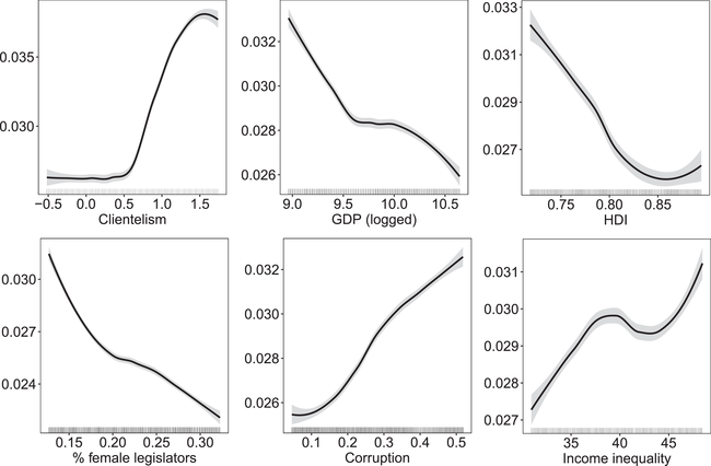
Figure 3. Partial dependence plots for the six most importance variables. Each panel provides the predicted change in unequal representation as a predictor is moved across its inter‐quartile range. Lines represent loess fits, with 95 per cent confidence intervals in grey, computed from random forest predictions across all imputation replicates. Rug plots are also provided along the
 axis to indicate support in the underlying data for these predictions. Note the differing axes in each panel.
The resulting relationships are largely consistent with theoretical expectations. Higher levels of clientelism, corruption and income inequality are associated with higher levels of bias in representation in favour of the affluent. Conversely, as levels of economic and social development and female representation increase, unequal representation in favour of the rich appears to decline. There are some nonlinearities in these relationships, but they nevertheless seem remarkably close to linear.
To quantify the magnitudes of these effects, Table 2 provides the change in the expected quantile of the dependent variable that results when each covariate is (separately) shifted from its 25th to its 75th quantile. For example, when clientelism is low, the gap in representation is predicted to be just above the empirical mean, in the 56th quantile. When clientelism is high, this gap is predicted to be in the 65th quantile, a shift of just over 8 per cent of the observed representation gap (before rounding). For an example to build intuition, this shift corresponds to the difference between Finland in 2014 (low clientelism) and Mexico in 1997 (high clientelism). On the other hand, when the human development index (HDI) is shifted from its 25th to its 75th quantile, the EMD drops from the 62nd to the 56th quantile. Although this shift may seem small in the abstract, it corresponds to the difference between the Dominican Republic in 2014 (low HDI) and Ireland in 2011 (high HDI).
Table 2. Effect magnitudes from the random forest

Predictions indicate the difference in the quantile of the dependent variable that results when the covariate is shifted across its interquartile range, as generated by simulating out of the random forests fit to each of the imputed data replicates.
As expected, the largest effects are found among the most important variables. None of the variables by themselves account for massive portions of the representation gap. But together, these variables explain a substantial amount, consistent with our expectation that unequal representation is multi‐causal.
Unequal representation in Western Europe
By painting in such broad strokes, with a comprehensive cross‐national dataset, our analysis may miss important variation among smaller subsets of cases. For instance, while factors such as clientelism, corruption and levels of development are important for predicting unequal representation globally, these variables may prove less important among the more developed democracies in Western Europe – where much of the comparative research on unequal representation is focused. In these countries, levels of clientelism and corruption are comparatively low and levels of development are comparatively high, particularly relative to Latin America.
To explore this possibility, we subset our data to include just Austria, Belgium, Finland, France, Germany, Greece, Iceland, Ireland, Italy, the Netherlands, Norway, Portugal, Spain, Sweden, Switzerland and the United Kingdom. We then rerun all of the same models described above and compute the same variable importance measures. The results of this exercise are presented in Figure 4.
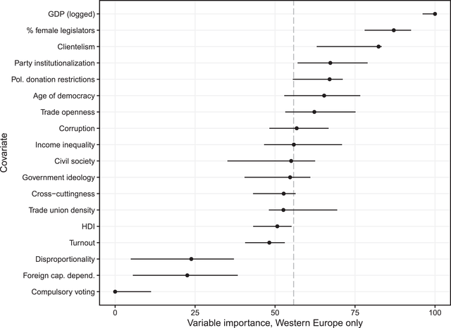
Figure 4. Variable importance in Western Europe. Each dot represents the mean variable importance, with lines for the interquartile range, across all imputation replications from the random forest model. Larger values indicate variables providing the model more information for predicting unequal representation.
Subsetting to just these developed democracies does change the results but not as much as one might expect. Economic development appears to be even more important for predicting the representation gap among Western European democracies than across our global sample. Corruption does drop off in importance but remains above average, while clientelism remains among the most important variables. Female representation also remains among the most important variables even within Western Europe. At the bottom end, disproportionality and compulsory voting remain among the least important variables, and other factors like globalization and government ideology continue to show middling or below‐average importance.
Three notable differences do appear. Party institutionalization, which showed a middling level of importance in the global sample, is one of the most important variables in the Western European subset. Unsurprisingly, HDI appears to matter much less in Western Europe. Perhaps most notably, given its prominence in studies of the United States, restrictions on political donations are vastly more important in Western Europe than globally.
On the whole, these results still suggest that economic conditions and governance are the most important areas for understanding unequal representation worldwide. While there are some differences between the more developed democracies in our dataset and the rest of the sample, most of the conclusions from the broader dataset hold also for this subset. Perhaps the most notable exception is that campaign finance and party institutionalization seem to matter more in Western Europe than they do elsewhere. Still, these results reassure us that the global patterns in the data are broadly worth pursuing for further theorizing and hypothesis testing, regardless of whether one is ultimately interested in understanding unequal representation in but one region of the world.
Understanding unequal representation
Political scientists are coming to grips with the finding that around the world, elected representatives sometimes better reflect the preferences of rich citizens. While there are on‐going debates about the extent of this bias in the United States, comparative research is remarkably uniform in uncovering such a bias, at least when it comes to economic issues. But we have few empirical studies that try to explain this bias. And those that do, focus on a single explanatory factor in isolation and often on a small number of countries.
Using a new dataset on mass–elite congruence around the world, matched to the relevant country‐year covariates, we have sought to begin to fill this gap. Our descriptive efforts here reveal that variables relating to economic conditions and governance are the most important for predicting affluence bias in representation. We find little support overall for hypotheses that affluence bias might be due to factors relating to political institutions, interest groups, or political behaviour, such as turnout.
This is but an initial exploration of the patterns in unequal representation around the world. Our study highlights factors that the data tell us appear to be most important in understanding differences in unequal representation over time and space. Our descriptive analysis relies on existing measures and on correlations in the data; we cannot draw conclusions from this about causal relationships among the variables. Still, this exercise should help guide future theorizing about this important research topic in democratic politics.
Broad studies of this kind are not without limitations. For one, we are limited by the kinds of measures that are available across time and space, though they surely do not exhaust the factors that might explain unequal representation. For instance, one possible explanation for affluence bias is that elected representatives misperceive the preferences of their constituents. Representatives' perceptions are an important link in the representational chain developed by Miller and Stokes (Reference Miller and Stokes1963). There are reasons to think that with the spread of opinion polls, representatives' information about public preferences could be more accurate (Geer Reference Geer1996), but there is also growing evidence of biases in how legislators and their staffs derive impressions of public opinion (Butler Reference Butler2014; Hertel‐Fernandez et al. Reference Fernandez, Mildenberger and Stokes2019; Broockman & Skovron Reference Broockman and Skovron2018). Another, related possibility is that elected representatives reflect better the preferences of the affluent because they themselves tend to be affluent, something that has recently received renewed attention (Carnes & Lupu Reference Carnes and Lupu2015; Carnes Reference Carnes2013). Neither of these possibilities lends themselves to the kind of cross‐national analysis we engage in here, but they surely merit further investigation.
There is also some comparative evidence that the poor and the rich may base their voting behaviour on different issue domains (e.g., Shayo Reference Shayo2009; De la O & Rodden Reference O and Rodden2008; Calvo & Murillo Reference Calvo and Murillo2019), which may explain why representation on the left–right dimension (our focus here) favours the affluent. If the rich care more about the economic issues captured by this dimension and the poor care more about other issues, then these inequalities may be a function of elected representatives simply reacting to issue publics. Again, while our empirical strategy is ill‐equipped to study this possible explanation, we hope future research considers it further.
Our analysis also focuses on congruence and on collective representation, two among multiple other dimensions of the broad concept of democratic representation. As we note above, these choices are driven both by theoretical interest – theories of representation ascribe substantial normative significance to both congruence and collective representation – and empirical tractability, given the availability of a broad comparative dataset. This of course leaves open the possibility that the explanations for the type of unequal representation we study would not generalize to other dimensions. Indeed, the extent to which representation itself is unequal may vary depending on the policy domain and type of inequality one measures. But our efforts here still point to useful directions for understanding why the aspects of representation that we study are unequal.
Acknowledgements
We presented our early results from this paper at Amsterdam, Geneva, Gothenburg, Princeton and Rice. We are grateful to these audiences for their helpful feedback. Lupu acknowledges generous support from the Unequal Democracies project (ERC grant 741538).
Online Appendix
Additional supporting information may be found in the Online Appendix section at the end of the article:
Table A1: Data sources
Table A2: Predictive performance
Figure A1: Partial dependence plots.
Table A3: Variable importance results under listwise deletion
Supporting Data S1


 x
x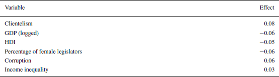


 Open access