Inventory management with carryover in the laboratory: going beyond the news vendor

Abstract

This paper considers a stationary model of inventory management in a rich setting in which unsold units carry over, in contrast with the full depreciation of unsold units that is implemented in laboratory studies of the news vendor problem. The model permits an array of costs associated with restocking, understocking, depreciation, financing, and holding inventories. The extra dimensions make it possible to hold the optimal inventory constant, while adjusting parameters that change the frequency of stockouts and the risks associated with storage and depreciation. This framework facilitates an investigation of factors that influence the nature and severity of behavioral biases observed in simpler news vendor settings. Optimal inventory decisions are derived and tested with a laboratory experiment. We consider four main questions in the inventory literature: the “pull-to-center” effect, the “recency” effect, the effect of increased up-front costs, and the effect of risk aversion.

1. Introduction

The news vendor paradigm, with full depreciation of any unsold units, has become a “workhorse” framework for laboratory studies of behavioral operations management. The underlying theory is conveniently simple and intuitive when demand is random and units can be purchased at a cost c and sold at a price p. Let q denote the inventory stock, and let F(•) denote the cumulative demand distribution, so an additional unit of inventory will sell with probability 1 – F(q). The marginal expected revenue of [1 – F(q)]p is equated to the marginal purchase price of c, to obtain the formula for the optimal inventory: F(q) = (p – c) / p.¹ If demand is uniform on [0, 1], for example, then F(q) = q, and the optimal inventory is the ratio of the profit margin to the product price (p – c) / p, a classic formula that is commonly known and that can even be found on Wikipedia.² In a laboratory experiment, the optimal inventory can be moved around by changing parameter values. A commonly observed pattern in news vendor inventory experiments is that order quantities tend to be too high when the optimal order is low relative to anticipated demand. Conversely, order quantities tend to be too low when the optimal order quantity is relatively high (Schweitzer & Cachon, 2000). This directional bias persists with scaled-up payoffs and reduced frequency of orders relative to demand realizations (Bostian et al., 2008).³

The news vendor problem is somewhat special in the sense that most inventory management settings are for products that do not fully depreciate, which introduces a range of costs associated with restocking, holding, and financing inventories. Moreover, the special features of the news vendor setting typically studied may have yielded seemingly general results that are constrained by the narrow range of situations considered. For example, the vast majority of news vendor experiments have been done with uniform demand distributions over a specified interval. As a result, holding the optimal inventory when it is low in the range of demand quantities will result in frequent stockouts, which could cause actual inventory choices to be above optimal levels. Conversely, holding the optimal inventory when it is high in the feasible range will result in frequent cases of “worthless” unsold units, which could cause actual inventory choices to be below optimal levels. Behavioral responses to recent outcomes, stockouts or unsold units, therefore, may result in a “pull-to-center” pattern between high and low optimal inventory treatments. This possibility has, of course, been recognized by researchers, who have specified and estimated models with “recency effects.” Such models are developed in Bostian et al. (2008), who also find evidence of a reinforcement bias in which participants tend to focus more on earnings from decisions previously made than on counterfactual earnings from decisions not made.

Instead of fitting a behavioral model to the simple news vendor framework, our approach in this paper is to specify an inventory model with a wide range of possible parameter variations that can be used to evaluate behavior in carefully specified treatments. In particular, we investigate several behavioral effects identified in the existing news vendor literature, for example, the related pull to center and recency effects. The pull-to-center effect refers to “the observation that people place order quantities that are between the expected‐profit‐maximizing quantities and mean demand” Beker-Peth et al. (2013). Brokesova et al. (2022) define it as “the observation that people order too few units when the per-unit inventory cost is relatively low and too many units when the cost is relatively high.” In our setting, the pull to center may be defined as the observation that orders tend to be above the optimal inventory level when the optimal inventory level is relatively low in the range of possible demands and below the optimal inventory level when the optimal inventory level is relatively high in the range of possible demands. We also elicit measures of risk aversion and consider their effects.

We replicate the pull-to-center effect in a general setting in which inventory carries over. One approach that is directly motivated by the previous paragraph’s discussion of recency effects is to hold the optimal inventory constant across a pair of treatments, while moving the stockout probability (at the optimal inventory) by changing the distribution of possible demand quantities. We also investigate whether decision makers are more sensitive to some cost factors, for example, the up-front cost of purchasing a unit of inventory, relative to other factors like the costs of holding inventory. This approach resembles the strategy used by Rapoport (1967) who investigated the impact of several variables in a multistage single-product inventory task, including storage costs and shortage costs.

The next section contains the derivation of optimal inventory stocks in a fairly general model, with the qualitative effects of risk aversion being derived in Appendix A. The third and fourth sections provide a description of the experiment procedures and the design of paired treatments. The fifth and sixth sections contain a sequence of results and support for those results. The seventh section presents a logit probabilistic choice model that is consistent with the observed pull-to-center effects, which are discussed more broadly in the final section.

2. Theory

Consider an inventory decision with discrete time periods, in which purchases are made at the start of a period at a unit cost of c, and sales revenues at a price of p per unit are received at the end. As before, let q denote the inventory stock, which will be a fixed target quantity for the stationary setting to be considered. The available stock (carried over or purchased) requires an inventory holding cost h per unit held during the period, including the period in which it is purchased. It is assumed that p > c + h to avoid the situation in which the optimal inventory is zero. Unsold units are depreciated at a rate of δ, so the fraction (1 – δ) of the unsold units constitutes the carryover prior to restocking at the start of the next period.⁴ We first characterize the optimal inventory policy in the absence of behavioral biases, under an assumption of risk neutrality. Appendix A contains a proof that the effect of an increase in risk aversion is to lower the optimal inventory stock, even when unsold units are not fully depreciated (i.e., with full or partial carryover).

To summarize the notation: q = target inventory level, D = random quantity demanded, c = cost of ordering a unit to add to inventory, p = retail price per unit sold, h = holding cost for each unit purchased or carried over from prior periods, δ = depreciation rate (fraction of inventory that is lost due to spoilage or theft each period). For simplicity, the depreciation rate is assumed to be fixed in the sense that it is independent of the age or “vintage” of an unsold unit.⁵

The distribution of exogenous demands is represented by a probability density function f(•) with cumulative function F(•). In the baseline treatments of the experiment to be reported, demand was uniformly distributed over the 100 integers from 1 to 100, which is easy to explain to participants. In this case, Pr(D ≤ q) = q / 100 and Pr(D > q) = 1 – q / 100, so a stockout should occur more frequently when the optimal inventory is low in the distribution of demand realizations. Stockouts might have behavioral consequences associated with regret, and therefore, we introduce a treatment that manipulates the demand distribution in a manner that moves the stockout probability at the optimal inventory level but holds the optimal inventory constant for different treatments. This permits us to isolate the effects of (nonoptimal) best responses to the most recent demand realization, that is, recency bias.

The firm’s payoff is calculated as the net revenue (price minus cost) for units sold, the first term on the right side of (1), minus the cost of restocking to cover depreciation of unsold units (second term), minus holding costs for a stock of q:

(1)\begin{equation}Payoff = {\text{ }}\left( {p\, - {\text{ }}c} \right)min\left( {q,D} \right)\,\,\, - {\text{ }}\left( {\delta c} \right)max\left( {q--D,{\text{ }}0} \right){\text{ }}--hq.\end{equation}

For example, consider a firm with a 10% depreciation rate that begins a period with a target inventory stock of 100 units and incurs a holding cost of 100 h. If the firm sells 60, the carryover to the next period would be 90% of the 40 unsold units, or 36, and the cost of restocking the 4 unit depreciation would be 4c. At the beginning of the next period, the firm would order 64 (cost of sales plus depreciation) to restore the total stock to 100. Assuming risk neutrality, it is straightforward to break the min and max expressions in (1) into separate integrals over the demand distribution. Maximization of the resulting expected payoff function yields the first-order condition for the optimal inventory stock, a condition that will be derived later in the proof proposition 1:

(2)\begin{equation}\left( {p - c} \right)\left[ {1 - F\left( q \right)} \right]\quad = \quad \delta cF\left( q \right) + h.\end{equation}

The intuition for this result can be seen by considering the consequence of stocking one additional inventory unit that will sell when demand exceeds the current stock, which occurs with a probability of 1 – F(q). Thus, the left side of (2) represents the expected net revenue for an additional inventory unit that sells with probability 1 – F(q), which is decreasing in q. An additional unit will remain unsold with probability F(q), so the first term on the right side of (2) represents the expected marginal cost of restocking for depreciation of unsold inventory, which is increasing in q. The final term on the right side represents the costs associated with holding an additional inventory unit. The optimal inventory condition in (2) can be solved for the probability of no stockout with optimal inventory:

(3)\begin{equation}F\left( q \right)\quad = \quad \frac{{p - \,c - \,h}}{{p - \left( {1 - \delta } \right)c}}\,\,\left( {optimal{\text{ }}no - stockout{\text{ }}probability} \right).\end{equation}

Note that the numerator of (3) is the price-cost margin for a unit that is sold, including replacement and holding costs. The denominator is the margin between the price and the carryover value (after depreciation) of a unit that is not sold. To summarize:

Theorem 1: With a stationary demand distribution F(•), the optimal inventory stock, q, under risk neutrality equates the probability of no stockout, F(q), to [p – c h)] / [p – (1 – δ)c], which is the ratio of the price-cost margin for a unit sold (including holding cost) to the price minus carryover-value margin after depreciation for a unit not sold. An increase in risk aversion reduces the optimal inventory stock.

Proof. The proof is based on the observation that any unsold unit at the end of the round is depreciated and valued at $\left( {1 - \delta } \right)$c, representing the cost reduction of returning the inventory to the target level q in the next period. There is no “next period” in the final period of an experiment, in which case this $\left( {1 - \delta } \right)$c amount is the preannounced redemption value for final inventory remaining. Let q = I + z, where I is the initial inventory at the beginning of the period and z is the order quantity that incurs a cost of zc on the far-right side of the expression below. The first and second terms show the sales revenue for the cases of no stockout and stockout. The third term shows the expected value of depreciated unsold inventory at the end. The term for holding costs depends on total inventory held, which is q (equivalently I + z).

(4)\begin{equation}p\mathop \int \limits_0^q xf\left( x \right)dx\quad + p\mathop \int \limits_q^{100} qf\left( x \right)dx\quad + c\left( {1 - \delta } \right)\mathop \int \limits_0^q \left( {q - x} \right)f\left( x \right)dx\quad - \;hq\, - zc.\end{equation}

One implication of this formulation is that the firm’s incentives are unchanged in the final period of an experiment if each unit of remaining inventory at that point is “redeemed” for c per unit after depreciation. The derivative of (4) with respect to the order quantity z is done using the condition that dq / dz = 1, since the initial inventory I is fixed. The effects of q in the limits of the first two integrals cancel out, and the effect of q in the upper limit of the third integral is zero since the integrand is zero at that point. The remaining derivative terms: $p\left[ {1 - F\left( q \right)} \right]\quad + c\left( {1 - \delta } \right)F\left( q \right) - h - c$, can be set to 0 and rearranged as (2) with marginal expected (net) revenue on the left and marginal costs on the right. The first statement of the proposition follows from the resulting optimal stockout probability in (3) and the maintained assumption that the price-cost margin is positive. The second statement is proved in Appendix A by comparing two utility functions, one of which has higher absolute risk aversion, – Uʺ(π) / Uʹ(π), for all possible payoff levels, π ■

For the uniform distribution used in some treatments of the experiment, F(q) = q / 100, so the optimal inventory determined by (3) is:

(5)\begin{equation}q\quad = \quad 100\;\;\frac{{p - c - h}}{{p - c + \delta c}}.\end{equation}

In the special case of full depreciation and no holding costs (δ = 1 and h = 0), the optimal inventory is given by the standard news vendor formula for a firm that purchases perishable units at a cost of c and resells at a price p: q = 100(p – c) / p. As the depreciation rate in the denominator of (4) decreases, optimal inventories are higher than the news vendor benchmark since unsold units have some value. In the extreme case of zero depreciation and no holding cost (h = 0 and δ = 0), the optimal inventory is 100, which prevents any chance of “stockout” in the absence of costs beyond the cost of purchasing at wholesale.

The result for risk neutrality in (3) is consistent with prior work on inventory management, for example, Porteus (2002). As far as we know, the risk aversion generalization is new, although risk aversion effects are well understood for the special case of the news vendor (full depreciation) case. See Eeckhoudt and Schlesinger (1995), who also derive an array of comparative statics results associated with demand risk and other parameter changes. In addition, Becker-Peth et al. (2018) hypothesize that risk aversion is associated with lower ordering quantities, which is confirmed by Becker-Peth and Thonemann (2018) for the news vendor case. For the discrete uniform demand distributions used in the experiment, the risk-neutrality predictions in (5) determined for the continuous demand can be verified by using a spreadsheet with 100 rows, one for each demand quantity D, and with a column for each of the possible values of q, the final inventory holding levels. Then (1) can be used to calculate the payoff for each cell (D, q combination), and the average of cells in each column determines the expected payoff for that inventory stock q. The resulting vector of expected payoffs traces out a quadratic curve that is maximized at the q value determined in (5). These calculations can also be used to evaluate payoff flatness and risk associated with possible treatments.

3. Experiment design

The model presented in the previous section contains an array of parameters that can be varied in an experiment. Our design has three sets of treatments, the Holding Cost treatments, which vary the holding cost parameter (low, medium, and high), the Demand treatments, which vary the median of the demand distribution (low, medium, and high in the interval of possible demands from 0 to 100), and the High Purchasing Cost treatment, which increases the cost of purchasing inventory and lowers the holding cost in a balanced manner (details to follow). In all treatments, the product price is held constant at $0.06, and the redemption values are set equal to the purchase cost c in order to avoid endgame effects. Since the news vendor problem with full depreciation has been the focus of so many investigations, we decided to use the other extreme with no depreciation, δ = 0, in all treatments.⁶ Finally, demand ranges from 0 to 100 in all treatments. Participants were informed of these endpoints, although the distribution of demand over this interval was not announced, which allows for testing the effect of observed demand on behavior.

3.1. Holding cost treatments

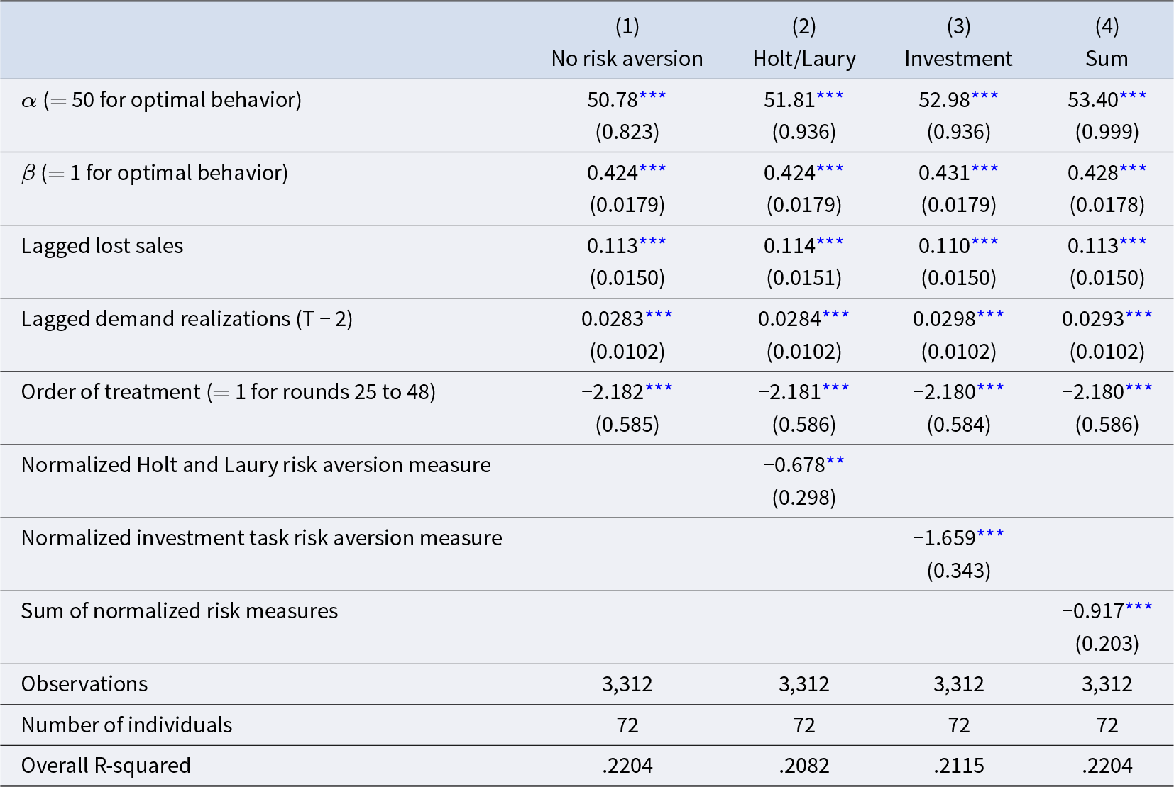
The standard way of evaluating a pull-to-center effect in a full depreciation (news vendor) setting is to vary the purchase cost c, but with δ < 1, changes in this cost affect both the numerator and denominator of the optimal no-stockout probability in (4), and therefore, we chose to vary the holding cost, h, to get sharper predictions. With no depreciation (δ = 0) and a price of 6, the ratio on the right side of (3) that determines the no-stockout probability is (6 – c – h) / (6 – c). The basic cost treatments maintain a price of 6 and a purchase cost of 2, while the holding h cost varies from 3 to 2 to 1, which yields optimal no-stockout probabilities of 0.25, 0.5, and 0.75, respectively, for the high, medium, and low holding cost treatments. With uniform demand on [0, 100], as represented by the diagonal dotted line in Figure 1, these no-stockout probabilities produce optimal inventory stocks of 25, 50, and 75, as indicated by the three dots with labels A, B, and C on that diagonal line. For example, when the holding cost is relatively high (at 3), the no-stockout probability is (4 − 3) / 4 or 0.25, as shown by the “Low Ratio” line in the figure. The intersection of this horizontal no-stockout line at 0.25 with the diagonal cumulative demand distribution in Figure 1 is at the point A, which yields the optimal inventory of 25 for this treatment. Lower holding costs produce higher no-stockout ratio lines, with intersections at points B and C in the figure. These three treatments are listed in the first three rows of Table 1, which shows the optimal inventory levels in the right column. By changing the holding cost from high (3) in treatment A to low (1) in treatment C, the optimal inventory switches from 25 to 75. This leads to our first hypothesis:

Pull-to-center effect: In this setting with full inventory carryover, observed inventory levels will tend to be too high when the optimal level is relatively low in the distribution of demands and will tend to be too low when the optimal level is relatively high.

Fig. 1 Optimal inventory levels for treatments A–F as intersections of cumulative demand distributions and horizontal no-stockout ratios determined by Equation (5)

Table 1 Summary of treatments (All without depreciation)

3.2. High purchasing cost treatment

Notice that the center point in Figure 1 had two labels, point B for the medium replacement and holding costs (c = 2 and h = 2), and point D at the same location. This second point was determined by raising the replacement cost and lowering the holding cost in a balanced manner to maintain a constant no-stockout probability at 0.5, determined by the intersection at the center of the diagonal line in Figure 1. The idea is to compare observed inventory levels for the two treatments with the same optimal inventory: treatment B with medium replacement and holding costs, and treatment D with high replacement costs (4) and low holding costs (1). A comparison of observed inventory stocks for these two treatments would help identify whether or not there is any bias associated with high replacement costs (incurred in the moment) as compared with holding costs (incurred later in the period and in subsequent periods in the event of no sale). This timing difference is, of course, an illusion, since replacement and holding costs are typically incurred in all periods in a steady state. Our second hypothesis is framed in terms of this possible bias, although the actual null hypothesis for the statistical test will be that average inventories are invariant to a balanced change in cost composition that does not alter the optimal inventory level:

Current cost bias: An increase in the current inventory replacement cost, balanced by an offsetting reduction in the inventory holding cost for unsold units, will reduce observed inventory levels, even when the optimal inventory level stays constant.

3.3. Demand treatments

The two kinked dashed lines in Figure 1 represent nonuniform demand distributions. For example, the upper dashed line, with a kink at an inventory of 25, has the property that half of the demand observations are uniformly distributed below 25, as indicated by the steep segment on the left side, and the other half are between 25 and 100, as indicated by the long flatter segment to the right. The optimal inventory of 25 is determined by the intersection of this upper kinked demand distribution with the middle horizontal line in Figure 1, which represents the no-stockout probability for medium replacement and holding costs, c = 2 and h = 2. Similarly, the lower demand distribution, with a kink at 75, intersects this middle horizontal line at point F, so the no-stockout probability is also 0.5 at the optimal inventory of 75 for that treatment (point F). The three diamonds (E, B, and F) on this horizontal line in Figure 1 can be thought of as treatments with three different median demands (25, 50, and 75), all with the same cost combination. Note that the middle point, at a median of 50, is for a uniform demand distribution with no kink. In the two kinked-demand treatments, the optimal inventory aligns with the kinks, which are the median demands. These kinks provide a tool for studying whether participants engage in demand-chasing behavior and whether this leads to a reduced pull to center. When the optimal inventory levels and the median demands are both at 25 (in the low kinked demand) or 75 (in the high kinked demand), chasing demand could lead to a decreased pull-to-center, as in both cases the optimal inventory is not at the center. This combination of treatments allows to study the pull-to-center phenomenon from a fresh angle and in settings, which should be neutral to the prevalence of this bias, as, in the kink demand treatments, the optimal inventory and the mean of the distributions are the same and, for the low and the high median treatments, not in the center of the distribution.

With a replenished inventory at the median of the demand distribution, the probability of a stockout (which might induce ex post regret for being short) is equal to the probability of having unsold units (which might induce regret for carrying too many units). Think of a “demand chaser” as someone who adjusts inventory in response to the most recent outcome, shortage or excess. In each of the kinked-demand cases, a myopic demand chaser is equally likely to be pulled down when demand is below the optimal inventory as to be pulled up when demand is above the optimal inventory. Thus, there is no systematic effect of observing stockouts or unsold units in the kinked-demand treatments. If a pull-to-center effect is due in part to myopic best responding to the directional effects of most recent demands for the uniform-demand treatments A and C, then the kinked-demand treatments E and F should result in lower deviations from optimal inventory levels (less pull to center), which leads to our third (alternative) hypothesis:

Recency bias: Any pull-to-center tendency that is observed when no-stockout probabilities are not constant at the optimal inventory levels (points A and C in Fig. 1) will be diminished when no-stockout probabilities are held constant (points E and F) so as to diminish recency effects.

4. Procedures

Participants were recruited from the University of Virginia for one-hour sessions. In total, 72 participants were included in 6 groups with 12 participants each.⁷ Each group made inventory decisions in two treatments (details to follow), that is, two sequences of 24 periods each.⁸ Participants were told the relevant holding and inventory purchase costs, and that demand would be between 1 and 100 inclusive, but they were only told that “The quantity that buyers are willing to purchase in a round is randomly determined.” A transcript of instructions is provided in Appendix B.

Cost changes between treatments were announced. In the kinked demand treatments, however, we observed slow learning and strong sequence effects in a pilot session, and therefore, we decided to use the same demand distribution for all 48 rounds when demand was kinked. For these sessions with a kinked demand, there was a statement that the probabilities associated with each possible demand quantity had not changed, even though the exact demand distribution was not announced (other than to reveal the minimum and maximum demands of 0 and 100, as had been done in the treatments with uniform demand).⁹

Each of the six labeled intersections in Figure 1 determines a treatment, and pairs of treatments are used to evaluate each of the three hypotheses provided in the previous section. Participants were recruited in groups of 12, with each group doing two treatments for 24 periods each, for a total of 48 inventory decisions. The first two groups encountered treatments with high and low holding costs, with high costs being encountered first for group 1 and second for group 2, as shown in the top two rows of Table 2. The right part of the table shows the cost parameters and the optimal inventory predictions with the first treatment listed on the left. For this test of the pull-to-center effect, the optimal inventories switch from 25 to 75 or vice versa. This pairing of extreme treatments was intended to determine whether deviations from optimal behavior for the same participants show up in different settings.¹⁰

Table 2 Treatments for each session, with payoffs in pennies

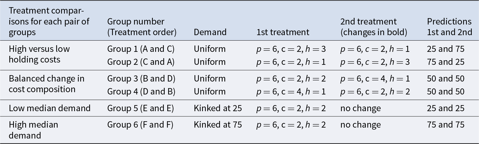
The middle part of the table, for groups 3 and 4, involves treatments with either medium replacement and holding costs (B) or with high replacement and offsetting low holding costs (D). The predictions for these two treatments are the same, with optimal inventories of 50 for each, as shown in the right column of the table. The bottom part of the table pertains to the treatments with a kinked demand structure that causes the median demand to be 25 when the optimal inventory is 25 (group 5) and to be 75 when the optimal inventory is 75 (group 6). Notice that there is no treatment change for either of these groups.

Each session began with a pair of financially motivated risk aversion measurements, with only one of the two methods being selected at random ex post to determine earnings. The earnings from these risk aversion tasks were not released until after all of the inventory decisions had been completed, at which time one of the investment tasks was selected at random to be payoff relevant. One of these measurements was a menu of six alternative investments with increasing risk for investments with higher expected returns. This menu, which is inspired by Binswanger (1981), will be explained in Section 6. The other measurement was the Holt and Laury (2002) procedure, which provides an ordered list of binary choices between safe and increasingly risky gambles as one goes down the list.¹¹ The purpose of obtaining risk aversion measures was to distinguish the effects of individual-specific risk preferences from general patterns of inventory adjustment. Total earnings averaged about $26 for the inventory decisions, $6 for the investment task, and $6 for the show-up fee, for a total of about $38.

5. Results

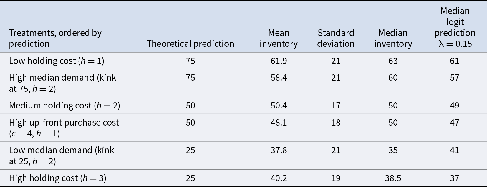
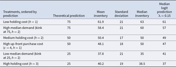
Table 3 shows treatments listed in order of optimal inventory from high to low, along with summary measures. Note that the measure of “replenished inventory” is the sum of the carryover from the prior period plus the order quantity for that period.¹² The top two rows show treatments for which the optimal inventory is high (75), which is the case with a low holding cost or with a high median demand (kink at 75). The middle two rows show treatments for which the optimal inventory is 50, which is in the middle of the demand distributions for those treatments. And the bottom two rows, with high holding costs or low median demands, show treatments with a low optimal inventory of 25. The mean and median inventories for the middle two rows are approximately 50, as predicted. For the other rows, the means and medians deviate from 50 in the right direction, but are less extreme than predicted. At the aggregate level, the median observed inventory is 63, with a low inventory cost, when it is predicted to be 75 (top row of Table 3). When the holding cost is high (bottom row of the table), the median inventory is 38.5 when it is predicted to be 25. Each of these medians is about halfway between the predicted level and the median demand of 50. The average inventory levels show a similar pattern. Our first result pertains to the pull-to-center effect of holding-cost variations shown in the top and bottom rows of Table 3.

Result 1. In a setting with full inventory carryover and a constant inventory purchase cost, increases in the holding cost reduce observed inventory levels as predicted, but replenished inventory levels tend to be too low when the optimal inventory is relatively high, and too high when the optimal inventory is relatively low. The observed “pull to center” is roughly symmetric for the parameters used.

Table 3 Replenished inventory by treatment: Summary statistics and risk neutrality predictions

Support: The decisions are independent across individuals, and therefore, we will use individual averages to determine the statistical significance of treatment differences. To allow for learning, we use averages for the last half of each treatment (last 12 rounds). If there were no pull to center, positive deviations from the predicted level would be balanced by negative deviations. Therefore, we will express these individual average inventories as deviations from the theoretical predictions in order to detect trends in deviations. If the treatment (high or low holding cost) were to have no effect on the bias, then the deviations would be the same, on average, in each treatment. In the presence of a pull to center, the deviations will tend to be negative when the inventory prediction is high (at 75), and the deviations will tend to be positive when the prediction is low (at 25). There are 24 participants who did both treatments (with treatment order reversed for half of them), so we have two vectors of 24 average deviations, one for each treatment. When the predicted inventory level is high (75), the average of the individual deviations is –13, and when the predicted inventory level is low (25), the average deviation is 12.8. This yields a treatment difference of 12.8 – (–13) = 25.8, with symmetry at the aggregate level. A simple way to proceed would be to test whether the individual deviation averages are higher for the high holding cost (low predicted inventory) treatment. This test is highly significant (p < .001) using a permutation test on the two vectors of deviations. A more appropriate test approach uses the fact that each person generates an average deviation for each treatment, a dependence that limits the possible permutations. This requires a matched-pairs permutation test, which considers the possible ways that the two observed deviations for each person could be permuted, where the p-value is the proportion of permutations that generate a treatment difference at least as large as the 25.8 difference that was observed. This test yields the same, highly significant, result (p < .001).

The conclusion that there is a universal pull-to-center bias must be qualified by the considerable heterogeneity among individuals (as noted previously by Lau and Bearden, 2014). We find that 50% of the participants had a mean replenished inventory between 25 and 50 in the High cost treatment and 54.16% of the participants had a mean replenished inventory between 50 and 75 in the Low cost treatment. Two of the people showed no deviation in either direction (optimal behavior) for one of the treatments and the predicted directional bias for the other treatment. Slightly more than half of the others (12 out of 22) exhibit a negative deviation when the predicted inventory is high and a positive deviation when the predicted inventory is low. Only one person exhibits the reverse “pull-to-extreme” pattern. All but three participants showed a lower (signed) deviation when the predicted inventory is high, but not everyone produced inventory levels in the center (25–75) range. Five participants were bold high-inventory types who showed positive deviations in both treatments, and another four were cautious low-inventory types with negative deviations in both treatments. Such systematic biases, upward or downward, could be due to risk preferences. Correlation between observed inventory levels and recent demand realizations (controlling for risk preferences) will be considered in the next section.

Next, we consider the treatments in the middle two rows of Table 3, one with medium costs (c = 2, h = 2) and one with high up-front purchase costs balanced by a reduction in holding costs (c = 4, h = 1) so as to leave the optimal inventory unchanged at 50 (assuming risk neutrality). Again, there were 24 participants who did these two treatments, with the order reversed for half of them.

Result 2: A doubling of the inventory purchase cost does not reduce observed inventory levels when it is balanced by a reduction in the holding cost by a factor of one-half, so as to maintain a constant optimal inventory. Thus, there is no clear evidence of a cost-composition bias for the parameters used.

Support: As before, we use the replenished inventory levels averaged for each individual for the last half of each treatment (periods 13–24 for treatment 1 and 37–48 for treatment 2). Even though average inventories are lower for the high purchase cost treatment, slight reductions in inventories might be due to risk aversion. In order to test the cost-composition hypothesis, we use a matched-pairs test again, which controls for individual risk preference differences. The data consists of 24 matched pairs of second-half average inventory levels. The second-half treatment averages are 48.96 for the baseline medium cost (c = 2, h = 2) treatment, and 46.08 for the high purchase cost (c = 4, h = 1) treatment, for a treatment difference of 2.875.¹³ The matched-pairs permutation test determines the proportion of permutations that yield a treatment difference as great (or greater than) this observed difference. This proportion is about 0.33 (two-tailed test) or about half that for a one-tailed test, so either way, the difference is not significant at conventional levels.

Next, we consider our third hypothesis, based on whether the pull-to-center pattern observed with uniform demands for high and low holding costs may be mitigated for demand distributions with a kink at the optimal inventory level. As noted previously, the idea behind this hypothesis is that most participants adapt and adjust instead of relying on complex mathematical calculations. Such participants may rely to some extent on the most recently observed demand when deciding on order quantities. Those who are subject to a recency bias (relying too much on the most recent experience) would appear to be “demand chasers,” raising inventory levels after stockouts and lowering them otherwise.¹⁴ In a low optimal inventory condition, orders would be pulled down when demand is below 25 and pulled up when demand is above 25. These effects balance out when the median demand is at 25, so we would not expect to see a consistent bias due to recency effects in this kinked-demand treatment. Similarly, in a high optimal inventory condition, replenished inventories are pulled down when demand is below 75 and are pulled up when demand is above 75, and these effects would be balanced when the median demand is 75.

The series of replenished inventories, averaged over all 24 participants in each treatment, is plotted in Figure 2. As noted before, inventories in the holding cost treatments and in the demand treatments show a pull-to-center effect relative to the theoretical predictions at 75 and 25 represented by the full horizontal line and short dash horizontal line at the top and bottom of the figure, respectively. The high purchasing cost treatment is reported with a long dashed line and tilted crosses.

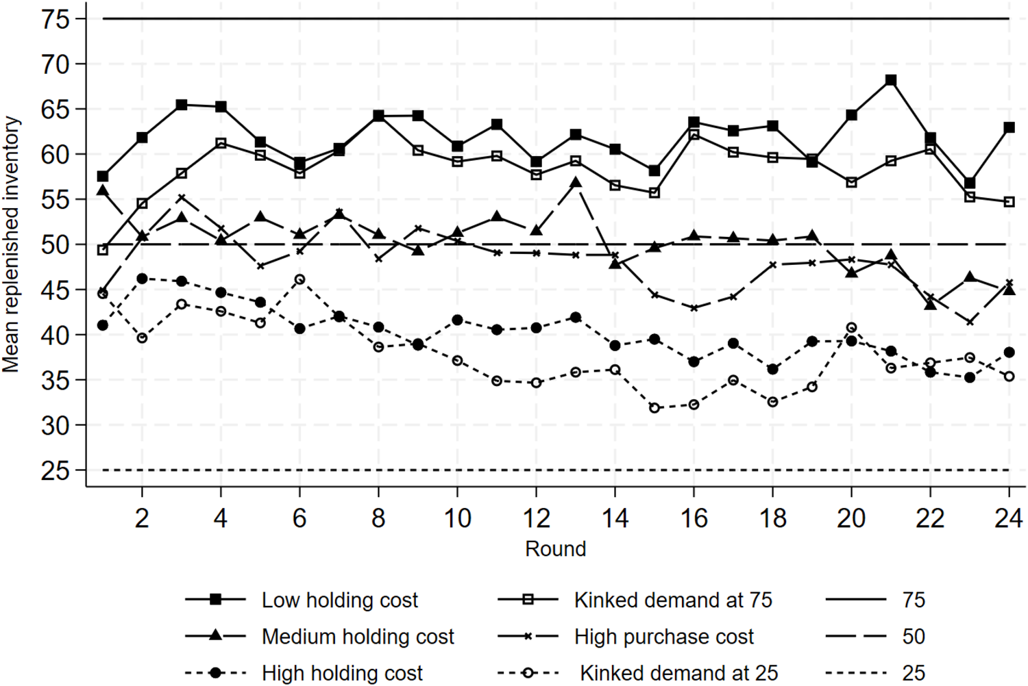
Fig. 2 Mean replenished inventory by holding cost variations and by kinked demand variations

Figures 3 and 4 further report that, consistent with the results of Brokesova et al. (2022) and Bolton and Katok (2008) in a news vendor setting, experience reduces the pull-to-center effect, but it does not make it fully disappear. These results indicate that the speed at which participants learn to maximize expected return differs across treatments, which is aligned with the analysis of Erev and Roth of the differences in learning speed (Erev & Roth, 2014).

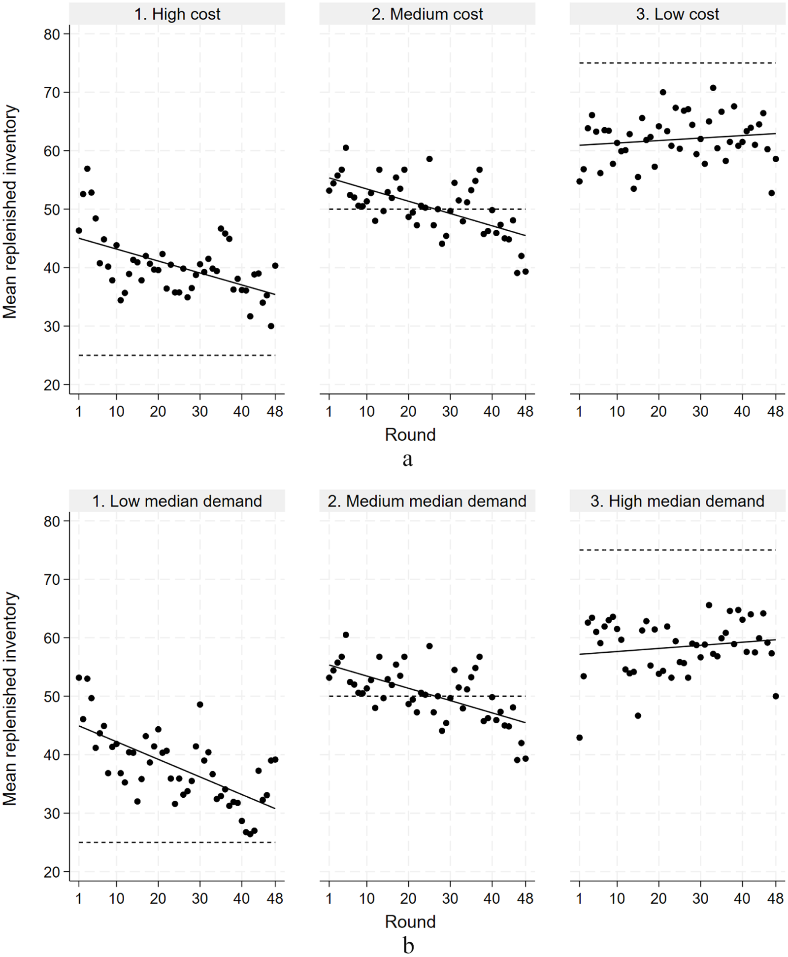
Fig. 3 (a) Mean replenished inventory by holding cost variations over the 48 periods. (b) Mean replenished inventory by median demand variations over the 48 periods

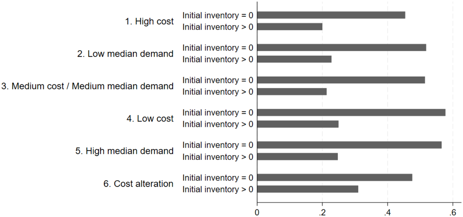
Fig. 4 Mean propensity to increase the replenished inventory after a round of stockout (initial inventory = 0) versus a round with carryover (initial inventory > 0)

As before, we will consider individual deviations, since one subject’s decisions are independent of another’s. We find that 71% of the participants had a mean replenished inventory between 25 and 50 in the low median demand treatment, and 63% of the participants had a mean replenished inventory between 50 and 75 in the high median demand treatment. The average inventory levels for the last half of each kinked-demand treatment (last 24 rounds in this case) are listed in the bottom two rows of Table 4. There was no treatment change for the kinked-demand treatments; the second-half data (rounds 45–48) are shown on the right side of the table, and there are only 12 participants in each treatment, as opposed to the 24 participants for prior (within-subjects) treatment comparisons. When the demand is kinked at 75 (bottom row), only one of these participants exhibits a positive deviation (77) from the prediction of 75; the other deviations are all negative. Conversely, for the treatment with a kink at 25, only one person, with an average of 19, exhibits a negative deviation relative to the prediction of 25.

Table 4 Average replenished inventories for the second half of each treatment

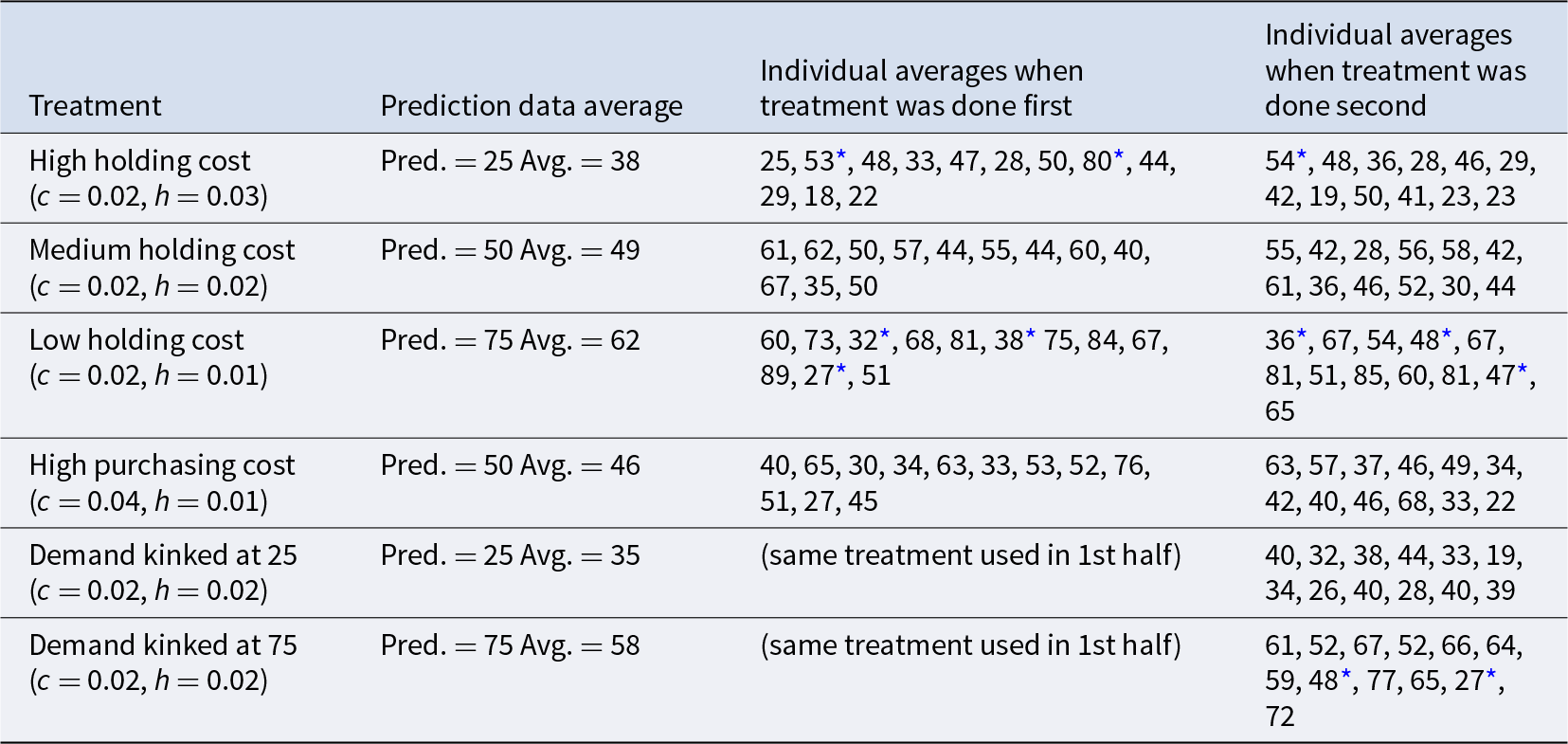
* Data averages on the “wrong side” of the midpoint inventory of 50.

In each case, we can reject the null hypothesis that the distribution is centered around the theoretical prediction.¹⁵ The more interesting question, however, is how the pull-to-center tendency for this treatment pair compares with that previously observed.

In the low median and high median treatments, we observe that participants whose replenished inventories are for a given round within 10 units of the previously observed demand realizations have replenished inventories that are closer to the optimal inventory. This results in a mean replenished inventory of 29.98 in the low median demand treatment (compared to 40.11 when not following demand), a mean replenished inventory of 61.53 in the High median treatment (compared to 57.69 when not following demand). The difference between these two groups is statistically significant, with p-values of .0000 and .0237, respectively, with Mann–Whitney tests.

In addition, we investigate whether participants have a propensity to increase their inventory after stockouts that is higher than after a round with carryover, that is, unsold items.¹⁶ We find that the propensity to increase the mean replenished inventory in a round after a stockout is doubled, as shown in Figure 5. These sequential dependencies (Plonsky et al., 2015) indicate that participants react to recent realizations of demand.

Result 3. Pull-to-center effects are not mitigated for the kinked-demand distributions that position the median demand at the high or low optimal inventory level.

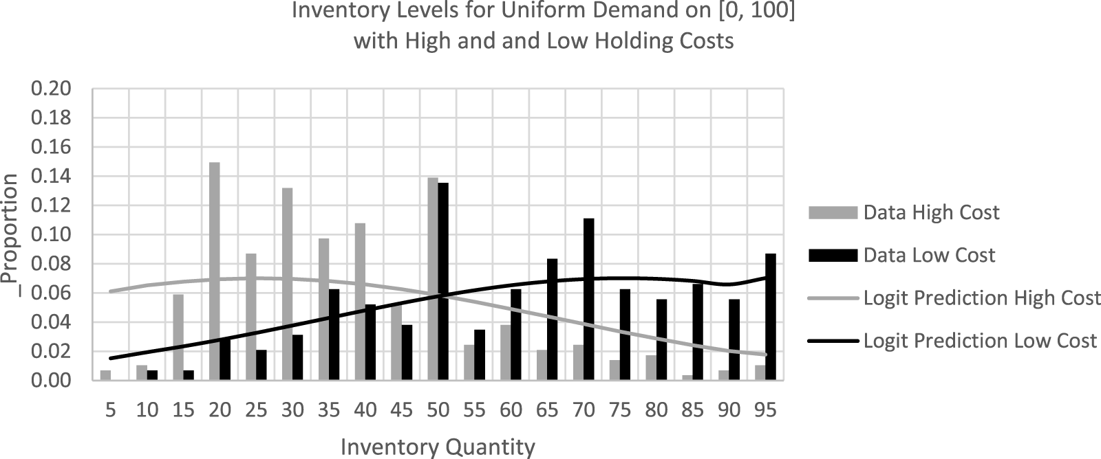
Fig. 5 Logit predictions and data distribution for high and low holding cost treatments

Support. To test the mitigation hypothesis, we first compare the individual averages for the two treatments with optimal inventories of 75. These averages are found on the right side of the low holding cost (third) row of Table 4 and on the right side of the bottom row. Despite the small difference in last-half average inventory levels (62 versus 59), the null hypothesis of no difference cannot be rejected (p = .66, 2-tailed permutation test).¹⁷ Nor is there a significant difference (p = .60) between the second-half inventory averages for the two treatments with theoretical predictions of 25: the high holding cost treatment and the treatment with kinked demand at 25. Thus, the kinked demand designs that align the median demand with the theoretical predictions do not attenuate the strong pull-to-center effect observed for the treatments with uniform demand.

6. Risk-aversion effects

The individual averages in Table 4 reveal considerable heterogeneity, which tends to blur pull-to-center effects. Documenting such heterogeneity helps assess the impact of having individuals decide on inventory levels, given that algorithms may be accompanied by humans for such decisions (Donohue et al., 2020). In this section, we will reevaluate this effect when individual measures of risk preference or aversion are used. We used two different choice menus to estimate the degree of risk aversion or preference.

The first measure (Holt & Laury, 2002) has 10 rows, each with a safe option that pays either $3.2 or $4, and a risky option that pays either $0.2 or $7.7, with the probability of the high payoff increasing from 0.1 in the top row to 0.2 in the second row, etc.¹⁸ A choice is made for each row, and then one of the 10 rows is selected at random, and the option (safe or risky) selected for that row is used to determine the person’s payoff. The number of rows in which the safe option is selected (usually they are contiguous) is used to infer the degree of risk aversion, with zero to three rows corresponding to risk preference, four rows for approximate risk neutrality, and five or more safe choices for risk aversion.¹⁹ Using this test, 48 of the 72 participants were classified as being risk averse, 16 were classified as being risk neutral, and 8 were classified as risk preferring.²⁰ We used the number of safe rows selected as the person’s risk aversion measure.

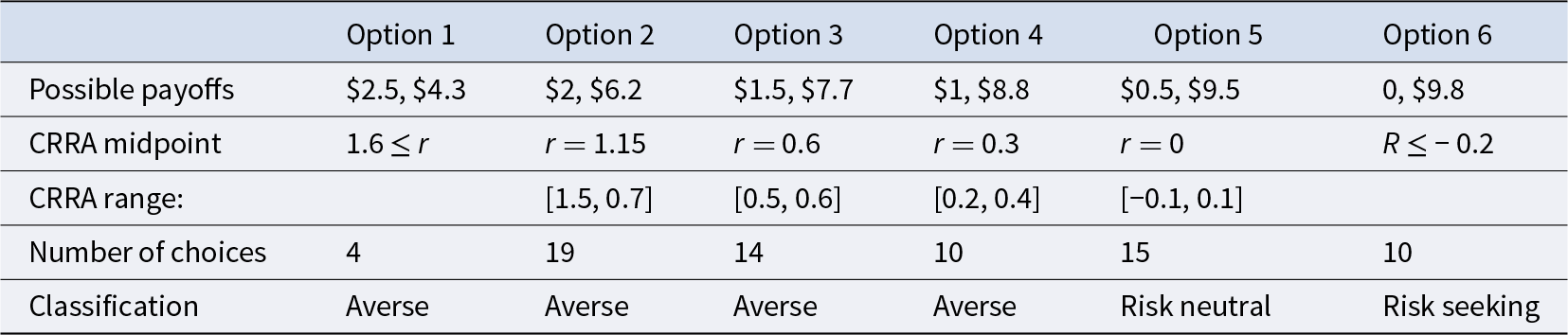
The simple binary choices in the Holt and Laury menu are quite different from inventory decisions, for which inventory increases result in more risk, with higher payoffs if demand is high, and low payoffs otherwise. Since high inventory orders are loosely analogous to allocating more resources to a risky asset, we use an investment task as our second measure, where the options correspond to investing a greater share of resources in a risky asset.²¹ We developed a modification of the Binswanger (1981) investment list for this paper by adjusting the nonlinear return parameter for the risky asset so as to generate equally spaced CRRA regions for alternative investments in the most relevant range. This second risk assessment task provides the subject with six alternative gambles or “investment options,” which are shown in the top row of Table 5, with increasing degrees of risk moving from left to right. Option 1, for example, involves equal probabilities of getting $2.5 or $4.3. Option 2 had a higher expected value but more payoff spread, and hence, more risk. For a utility specification of constant relative risk aversion (CRRA), that is, u(x) = x ^1–r / (1 – r), most participants are classified as having r measures in the range from 0 (risk neutrality) to about 0.6.²² The high and low payoffs used in this table were adjusted so that the CRRA intervals for Options 3–5 were equally spaced in this range, as can be seen from the “CRRA range” and “CRRA midpoints” rows in the table.²³ The CRRA midpoint for Option 5, the range [–1, 1] is symmetric around r = 0, which corresponds to risk neutrality. Payoff sums, and hence expected payoffs, increase moving from left to right, except that Option 6 has a lower sum and lower expected value than Option 5, and hence, only a risk-preferring person would select that option, based on the higher payoff spread it offers. The final row shows the distribution of options selected by the 72 participants, which has an average of 3.6, indicating moderate risk aversion. The number of the option selected is used in our subsequent analysis with this measure.

Table 5 Investment tasks with equally likely payoffs and risk preference classifications

To assess the effects of risk aversion on deviations from theoretical predictions, we estimate the panel regression model: ${\text{In}}{{\text{v}}_{i,t}} = \,{\alpha _i} + \beta {\text{De}}{{\text{v}}_{i,t}} + \,\gamma {\text{Lost sale}}{{\text{s}}_{i,t}} + \eta {\text{Lagged demand }}{\left( {{\text{T}} - 2} \right)_{i,t}} + \,\theta {\text{Order of treatmen}}{{\text{t}}_{i,t}} + \iota {\text{Ris}}{{\text{k}}_i} + {u_{i,t}}$, where Inv is the replenished inventory level, Dev is the deviation of the theoretical prediction (25, 50, or 75) from the midpoint of 50, Lost sales²⁴ is the difference between replenished inventory and demand when this difference is less than 0, LaggedDemand is the demand at the one before last period (T – 2),²⁵ Order of Treatment is whether the treatment was played first or second (with 1 for periods 25 to 48), Risk is the risk aversion measure (in columns (2), (3), and (4)), and u is the random effect specification. The prediction of 25 for the low-inventory treatments determines a Dev value of –25, the prediction of 50 determines a Dev value of 0, and the prediction of 75 determines a Dev value of +25. The optimal behavior is characterized by the parameters $\alpha = 50$ and $\beta = 1$, and a pull-to-center effect is characterized by the parameters $\alpha = 50$ and 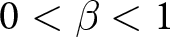$0 \lt \beta \lt 1$. In particular, the Lost sales variable picks up the opportunity cost associated with the units that could not be sold, but they were not in the replenished inventory.

The panel regression results are reported in Table 6 with separate regressions without risk aversion measures (Model 1) for each of the two risk measures,²⁶ the Holt and Laury measure (Model 2) or the Investment measure (Model 3) and the sum of both risk profiles (Model 4). The asterisks in the table represent significance levels for differences from zero. Since all of the β estimates are closer to zero than one, the β estimates for all equations are also significantly different from 1 (p < .01), which indicates a pull to center in all cases. Lost sales and the one before last previous demand realizations (T – 2) have a significant positive impact on replenished inventory. The positive coefficient for lost sales indicates that replenished inventory increases as lost sales become less negative, that is, closer to zero. The impact of the order of treatments is statistically significant. Increases in risk aversion measures are associated with lower inventory levels for all three measures. An additional safe choice in the Holt and Laury measure or a safer portfolio in the Investment measure would lead to both statistically and economically significant decrease in the replenished inventory, as predicted by theory.

Table 6 Panel regression results by risk measure

*** Standard errors in parentheses. *** p < .01, ** p < .05.

7. Probabilistic choice and pull to center

Our kinked demand treatments were designed to reduce the central tendencies in a non-news vendor setting with no depreciation of unsold units. In addition to the panel regressions shown in Table 6, we ran regressions separately for the high and low holding cost treatments and for the high and low kinked demand treatments. The estimated pull-to-center parameters (analogous to the β parameters in Table 6) were highly significant and approximately the same in both treatment pairs (0.434 in the cost treatments and about 0.42 in the demand treatments, where 0 is no pull and 1 is optimal). Thus the pull to center in our setup is alive and well, even after controlling for risk aversion and recency, and even after using kinked demands to pull the median of the demand distribution out from the center toward the high and low optimal inventory levels (corresponding to the high and low kinked demands).

At first we were surprised and disappointed by the persistence of pull-to-center effects in the kinked demand treatments, but a closer analysis of the expected payoff functions for these treatments revealed an interesting similarity: the expected payoff functions have a longer “tail” on the right side of the maximum when it is at 25 (high holding cost and low kinked demand), and the expected payoff functions have a longer tail on the left when the maximum is at 75 (low holding cost and high skewed demand). In each case, the expected payoffs are fairly flat around the optimum, so that deviations are not costly and are obscured by the randomness in demand and feedback. But there is more “room” for upward deviations in the treatments with low optimal inventories at 25, and more “room” to downward deviations with high optimal inventories of 75.

There is, of course, a lot of randomness in the data, due to a variety of factors, including complexity, confusion, or “bracketing” of attention on subsets of the perceived payoff landscape. Here, we use a simple logit probabilistic choice function to model the observed distributions of replenished inventories as functions of the expected payoffs. Recall that the expected payoff is essentially the price-cost difference times the minimum of the realized demand and replenished inventory, minus the holding cost. Sensitivity to expected payoffs is determined by the magnitude of a logit precision parameter, λ. The resulting choice probabilities for a choice of x are proportional to an exponential function of the expected payoff, weighted by λ: ${e^{\lambda \pi \left( x \right)}}$, where π(x) is the expected payoff for a replenished inventory of x. These exponential functions will sum to 1 if we divide by the sum of exponentials over all possible inventory choices from 1 to 100. These probability calculations are straightforward but tedious. We constructed a spreadsheet with 100 rows (one for each demand) and 101 columns (1 for each inventory level), using demand probabilities for the uniform or kinked demand setup. The elements in each column were weighted by the appropriate demand probability and summed to determine expected payoffs, which in turn were used to calculate the logit probability predictions.

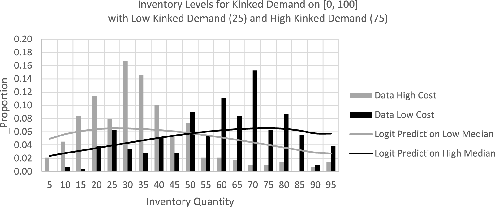
The logit explanation has more plausibility if the same logit precision parameter that explains the upward pull to center when the optimal inventory is low can also explain the downward pull in the opposite situation. Although the precision might be lower for the more complex kinked demand distribution, participants got more experience in the kinked demand sessions, and therefore, we use the last half of the data. The logit choice distributions shown by the smooth lines in Figures 5 and 6 were constructed with the same parameter value, λ = 0.15.

Fig. 6 Logit predictions and data distribution for high and low kinked demand treatments

Even though the data bars exhibit a fair amount of lumpiness at focal points in these figures, the logit parameter was selected so that the medians of all four treatment distributions are quite close to the observed median inventories. To see this, compare the medians of the logit distribution predictions in the right column of Table 3 with the data values shown in the mean and median columns in that table. To conclude, the observed pull-to-center tendencies with high or low optimal inventories (at 25 or 75) seem to be due to the shapes of the expected payoff functions that determine the logit prediction lines in Figures 5 and 6. These logit predictions have more density on the inside (center side) of the optimal inventory than on the outside of the optimal inventory. This result is consistent with the service contract treatment in Bolton et al. (2022), which changes the slope of the expected payoff, reducing the pull-to-center effect.

8. Conclusion

This paper proposes a general framework for studying inventory decisions that accounts for purchase and holding costs, and different degrees of depreciation that range from full depreciation (news vendor) to the full carryover used in the reported experimental test.²⁷ On the one hand, using such settings in laboratory research may pose a challenge as participants face more elaborate instructions and a more complex problem. On the other hand, a rich set of payoff options enables us to stress test results from the literature obtained in simpler settings, for example, the workhorse news vendor game. This framework can help document the impacts of individual heterogeneity as well as those of contextual and behavioral factors that are considered to be central in the current research agenda of operations decisions (Atasu et al., 2020; Caro et al., 2020; Donohue et al., 2020).

We find that replenished inventory decisions with full inventory carryover are directionally consistent with expected payoff-maximizing predictions but that, in the aggregate, the pull-to-center effect in the news vendor setting extends to our specification of this more general setting. Our paper contributes to the literature that studies the impact of the structure and complexity of the task on the prevalence of the pull-to-center bias. Zhang and Siemsen (2019) perform a meta-analysis of the experimental literature on the news vendor game and find that, although confirmed and very stable across studies, the pull-to-center effect varies significantly from study to study, underlying the importance of design aspects of the experiment. Although not done in a news vendor context, our study shows that the pull to center extends to more complex settings with holding costs and without full depreciation. Interestingly, Brokesova et al. (2022) report a pull-to-center effect in a price-gouging game that is “mathematically isomorphic” to the news vendor setting. They interpret their result as driven by structural aspects of their task rather than context-specific explanations pertaining to inventory management. Further research is needed to determine which economic settings are conducive to the pull-to-center effect and to study whether it is a fundamental attribute of human behavior.

Moreover, we observe that the pull-to-center pattern persists even when kinked demand structures are used to ensure that the median demand matches the expected payoff-maximizing inventory, so that recency effects of previous-period stockouts and surpluses are balanced. The fact that the recency bias does not reduce substantially the pull-to-center effect suggests that there may be an underlying explanation that is potentially more profound than a behavioral bias; individuals may want to balance the two objectives of meeting demand, which pulls their replenished inventory up, and of minimizing costs, which pulls their replenished inventory down, which leads to pull to center when the optimal replenished inventory is not at the center. A closer examination of the expected payoff functions revealed asymmetrical payoff distributions. When the optimal inventory is 25, the expected payoff function has a longer tail on the right, which is consistent with upward deviations. When the optimal inventory is 75, the expected payoff function has a longer tail on the left, which is consistent with downward deviations. The fact that the payoff region around the optimum is flat lowers the cost of deviations from optimality. The observed pull-to-center behavior is modeled using a logit probabilistic choice function. The model captures the median tendencies for all treatments, despite visible data lumpiness at focal points, and it explains both the observed upward pull and the downward pull from optimality. This result is consistent with the service contract treatment in Bolton et al. (2022), which changes the slope of the expected payoff, reducing the pull-to-center effect.

There is considerable heterogeneity across individuals, and we developed an investment task to measure individual risk preferences. This measure is closely related to the classic Binswanger (1981) menu, but it is structured to provide equally spaced intervals of constant relative risk aversion in the relevant range. Consistent with the literature (Eeckhoudt & Schlesinger, 1995; Van Mieghem, 2007), we show that, in our setting, risk aversion measured in this manner leads to lower optimal inventory levels, and we observe that risk-averse participants do carry lower inventories in the treatment variations caused by cost differences.