1 - Introduction

Summary

A brief overview and description of the atmospheric lidar measurement technique is followed by the structure of the atmosphere in terms of the troposphere, stratosphere, and mesosphere, as it is usually presented in atmospheric science and meteorology. The atmosphere is then described in terms of lidar observables at all altitudes, including water vapor; trace gases; clouds; several other kinds of particulate matter; and metal atoms, as well as density, temperature, and winds. Examples of lidar measurements include tropospheric and stratospheric ozone, greenhouse gases, other pollutants, tropospheric and stratospheric aerosols, polar stratospheric clouds, and atoms of sodium, potassium, calcium, and iron in the mesosphere. Finally, the structure and contents of the book are described, and suggestions for further reading are given.

Lidar (light detection and ranging) is an optical remote sensing technique used to measure properties of the atmosphere at long ranges without direct contact. Because a lidar system transmits pulses of laser light, the atmospheric measurements are functions of range, where the range is calculated from the pulse time-of-flight multiplied by the speed of light. Lidar is a very powerful tool for atmospheric remote sensing. No other active remote sensing technique can measure as many parameters as lidar.

1.1 The Atmospheric Lidar Technique

A basic lidar system is illustrated in Figure 1.1, where the laser emits pulses of light in a narrow beam into the atmosphere toward an opaque cloud. The receiver telescope collects backscattered photons and concentrates them onto a photodetector that converts the photons into an electronic signal. If that signal is plotted versus time, it will have the characteristics shown graphically in the box on the right: For short ranges, the signal will be zero, because none of the scattered photons can get through the receiver optics to reach the detector. At intermediate ranges, the signal is caused by backscatter from molecules, and it rises suddenly to a peak, from which it falls rapidly, until a second peak appears due to a strong signal caused by backscatter from the water droplets in the cloud. After the cloud, the signal returns to zero because the laser light cannot penetrate an opaque cloud, so no laser light is received from ranges beyond it.

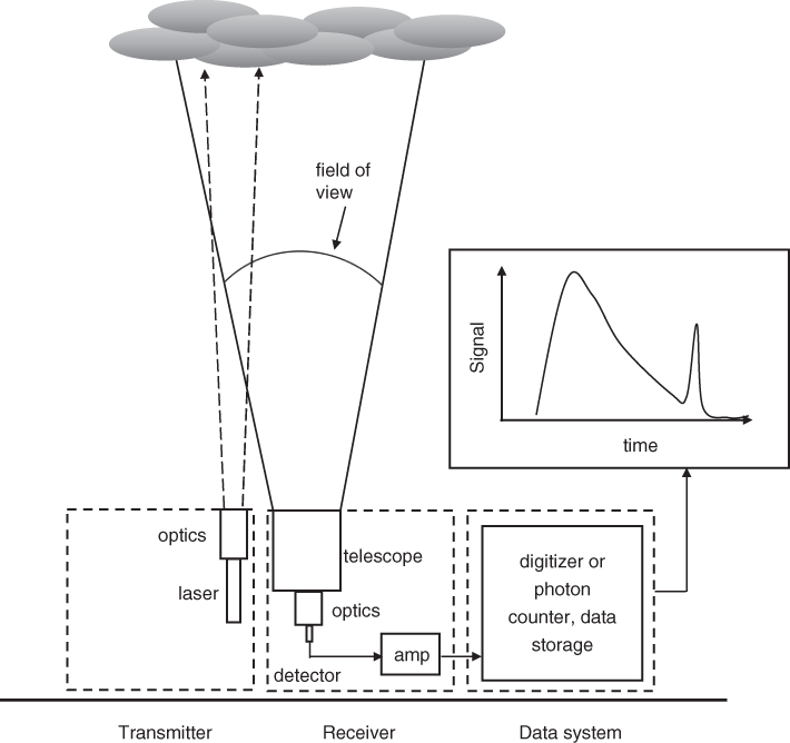
Figure 1.1 A basic lidar system. The lidar has three main components: a transmitter, a receiver, and a data system that acquires a transient electronic signal versus time, for each laser pulse.

In practice, the time axis shown in Figure 1.1 is always converted to range, by using the formula distance = velocity × time, where the velocity of light $c$ is 3 × 10⁸ m/s. The light must travel out and back, so the distance $2R$ is equal to $ct$ for a time $t$, and the lidar range $R$ is therefore $ct/2.$ For example, a time of 1 µs corresponds to a lidar range of 150 m. The lidar signal is often referred to as a transient waveform because it occurs in such a short time. The lidar signal is discussed in detail in the chapters that follow, but for now, it is sufficient to note three features: (1) a lidar system always has a nonzero minimum range; (2) the signal tends to span a very large dynamic range; and (3) the time duration of the signal is very short, generally less than 1 ms for ground-based lidars.

1.2 Structure and Composition of the Atmosphere

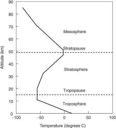
To appreciate the wide variety and value of lidar measurements, we must understand the structure and composition of Earth’s atmosphere. The atmosphere is conventionally described as a set of concentric spherical shells (troposphere, stratosphere, etc.) where the shell boundaries, known as pauses, are determined by inflections of the temperature profile, as shown in Figure 1.2. Clouds, convection, and weather phenomena are primarily in the troposphere, whereas there is much less vertical mixing in the stratosphere. The mesosphere is free of aerosols, and it was a poorly known region until remote sensing measurements became available. The thermosphere lies above these layers, from roughly 100 to 500 km, where the temperature rises rapidly with altitude and atmospheric gases may be ionized. From the ground all the way up to the top of the mesosphere at 100 km, the atmospheric gases are well mixed and neutral. Being well mixed means that air is always 78% nitrogen, 21% oxygen, and 1% argon, with smaller amounts of other gases, including 0.04% carbon dioxide (CO₂) and highly variable amounts of water vapor. Being neutral means that the concentration of ions is negligible in this altitude region.

Figure 1.2 The structure of Earth’s atmosphere. The conventional description of the atmosphere in terms of spherical shells is illustrated using the temperature profile data in the U.S. Standard Atmosphere, 1976 [1].

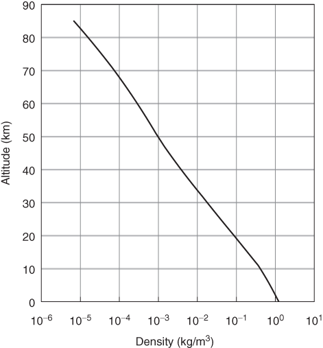
The decrease in air density with altitude is nearly exponential, and it decreases by six orders of magnitude between the ground and 100 km, as indicated in Figure 1.3, where the density scale is logarithmic. In geoscience, altitude is usually plotted on the vertical axis even though it is an independent variable, so this convention is followed in Figures 1.2 and 1.3. In lidar, signals are often plotted with range on the horizontal axis, as in the Figure 1.1 inset, but reduced data products in the form of altitude profiles are usually plotted using the geoscience convention. Modeled lidar profiles are plotted both ways.

Figure 1.3 Air density versus altitude. The air density profile is from the U.S. Standard Atmosphere, 1976 [1].

1.3 Atmospheric Lidar Applications

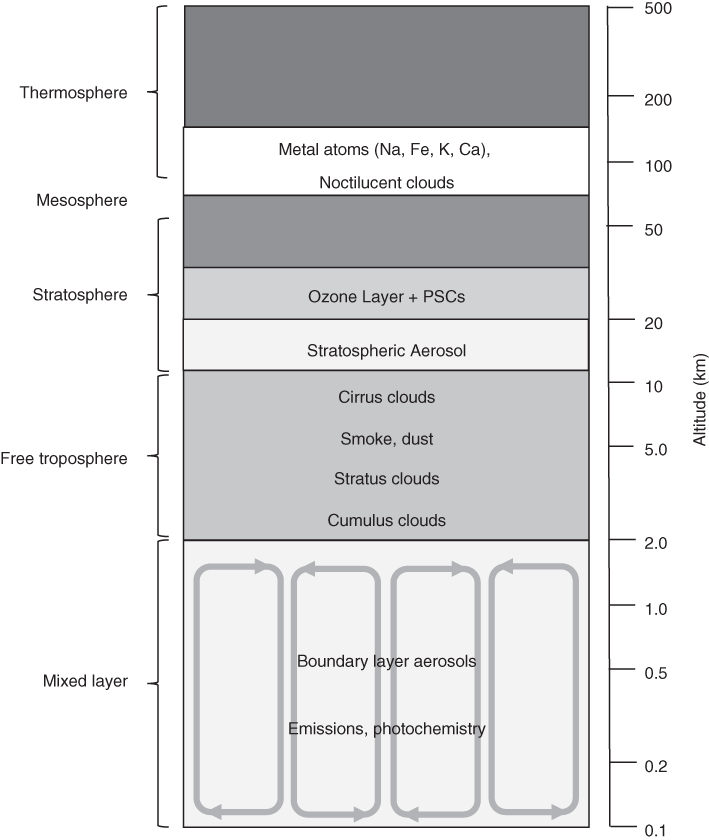
Figure 1.2 describes the atmosphere in terms of the conventional spherical shells of atmospheric science and meteorology, with a typical temperature profile. However, the lidar point of view is much more complex, as illustrated in Figure 1.4, because the atmosphere contains important observable constituents at all levels, including both trace gases and solid and liquid particles of matter. Lidar systems have been developed to measure all the constituents shown in Figure 1.4 as well as winds and temperatures. Some of those lidar measurements are briefly described in the following sections.

Figure 1.4 Lidar observables in the atmosphere. The main constituents that are measurable with lidar systems are shown for the various regions of the atmosphere. Note that the altitude scale is logarithmic.

1.3.1 Troposphere

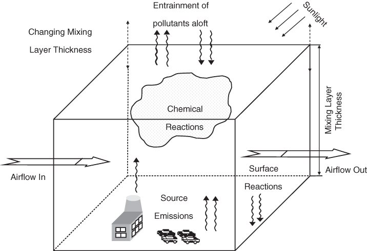
The troposphere is where virtually all human activity takes place. It has two distinct regions: the mixed layer, which is typically 1–2 km thick, and the free troposphere, where the word “free” refers to unimpeded winds. The greatest source of aerosols is at Earth’s surface, and those aerosols are carried upward by convection in the mixed layer. Photochemistry related to air pollution also occurs in the mixed layer, producing both ozone (O₃) and additional aerosols. Industrial emissions of pollutants occur at the surface, and those pollutants are diluted by the mixing action in this layer. Ozone and smog are major components of bad air quality, which is a regional hazard to human health often associated with urban areas. Some industrial emissions such as mercury (Hg) find their way into the environment and consequently into the food chain, again presenting a health hazard. Lidar techniques have been developed to provide information for managing all these issues. As shown in Figure 1.5, urban air-quality problems are intrinsically time varying and three-dimensional (3-D), depending on the mixing layer thickness, the emission rates of pollutants, prevailing winds, photochemical reactions, and entrainment of pollutants or their precursors in the free troposphere. Urban areas often have arrays of surface air-quality sensors to monitor the air that people breathe, but a detailed understanding of air quality can only come from measurements throughout the 3-D volume, which are difficult to obtain. For this reason, periodic air-quality measurement campaigns employ suites of ground-based and airborne instruments that usually include lidars because of their long-range measurement capability.

Figure 1.5 The three-dimensional nature of urban air quality. In any volume of the mixing layer, there are many sources and sinks for pollutants. All the factors shown tend to be time varying.

Lidar techniques are also being employed to monitor the related but much larger problem of global climate change. Although Earth’s climate does have natural periodic changes on geological timescales, as shown by phenomena such as ice ages, man-made emissions of certain gases and aerosols are introducing unusual changes to Earth’s energy balance. Without an atmosphere, the average temperature of our planet would be about 260 K, which is below the freezing point of water. The actual average temperature is a much more habitable 295 K because of the greenhouse effect, which is caused by atmospheric gases with strong absorption bands in the infrared region of the spectrum. The incoming and outgoing radiations are in a delicate balance: The sun’s irradiance outside the atmosphere (known as the solar constant) is about 1,400 W/m², and climate-changing imbalances are of the order of 1 W/m². Around 30% of the solar radiation (averaged over the globe and all seasons) is scattered to space by the atmosphere, land, and oceans. The remaining 70% is absorbed, and an equal amount of power escapes to space as thermal radiation. Both scattering and absorption of solar radiation in the atmosphere are highly dependent on aerosols and clouds, and small changes in the amounts or the optical properties of aerosols and clouds cause significant changes in the energy balance. In addition, aerosols cause an indirect change by influencing the formation of clouds and their ability to scatter sunlight. Lidar is an essential tool for studying and monitoring many of these competing effects.

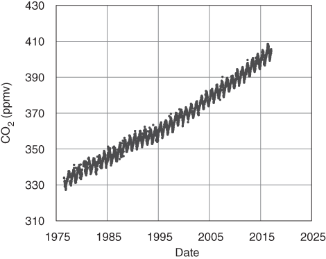
Of the absorbed 70% of the incoming sunlight, around 20% is absorbed in the atmosphere and the remaining 50% is absorbed at the surface. Much of the latter is reradiated upward as thermal radiation. However, only 6% is radiated directly to space, and the rest is absorbed by clouds and greenhouse gases (GHGs), of which the most important are water vapor, CO₂, methane (CH₄), and nitrous oxide (N₂O). The concentrations of the last three are increasing rapidly due to human activities. Since the start of the industrial revolution, CO₂ has increased by almost 50%, and its rate of increase is accelerating, as shown in Figure 1.6 [2]. As of this writing, half of the CO₂ humans have ever generated has been put into the atmosphere in the past three decades. CH₄ concentrations have more than doubled, and the greenhouse effect of CH₄ is 25 times that of CO₂. GHGs are already causing measurable climate changes, and the continued rise in their concentrations can lead to environmental catastrophes. The natural “sinks” that remove both natural and man-made gases are not understood, but the effects are already apparent. For example, CO₂ is being absorbed by oceans and land areas much faster than models predict, but there is great concern that the current absorption rate will not be sustained in the future. Carbonic acid (CH₂O₃) produced by CO₂ dissolving into sea water has already increased ocean acidity by 25% over the past two centuries, affecting the survival of many marine animals at the bottom of the food chain. As industrialized nations attempt to grapple with this situation, a need has arisen for monitoring GHG concentrations and emission rates globally. In response to this challenge, the international lidar community is pioneering a suite of techniques to monitor GHGs in Earth’s atmosphere, in which ground-based, airborne, and spaceborne measurement platforms all have applications.

Figure 1.6 Monthly mean CO₂ mixing ratios measured at Mauna Loa, Hawaii, known as the Keeling Curve. The jagged appearance is due to seasonal variations. The CO₂ concentration was in the 260–280 ppm range during the 10,000 years, leading up to the industrial revolution. Data are from [2], used by permission.

In the free troposphere, both aerosols and trace gases are transported over long distances, so they cause environmental harm far from the source of pollutants. For example, nitrogen dioxide (NO₂) is a precursor for ozone, but local regulations to control its concentration are not an effective strategy in the eastern U.S. because so much of it is transported from other regions upwind. The situation with sulfur dioxide (SO₂) is similar – once it gets into the free troposphere, it is transported by the prevailing winds, causing acid rain over wide geographical areas. Smoke from forest fires and ash from volcanic eruptions can also rise into the free troposphere and be transported to thousands of kilometers, causing widespread air-quality problems as well as hazards to aviation. Ground-based and airborne lidar systems are used to monitor and understand the transport of all these pollutants.

Several lidar techniques have been developed for measuring wind speed, which is a key parameter for weather forecasting and aviation safety. Wind lidars are in use at airfields to monitor local winds near the ground and to detect wake vortices, which are serious hazards to small aircraft. Studies have shown that measurements of the global wind field are the most important missing input for weather forecasting, and for this reason, spaceborne wind-profiling lidar technology is being developed in both Europe and the U.S.

1.3.2 Stratosphere

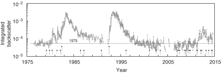
The stratosphere lies above the troposphere. As the name suggests, this region is stratified, meaning that there is much less vertical mixing than in the troposphere, but the stratosphere contains important layers from the lidar point of view. The stratospheric aerosol layer is mainly tiny drops of sulfuric acid, although it also contains ashes of meteors that burned up much higher in the atmosphere. This aerosol layer is constantly being depleted as the aerosols fall into the troposphere and become entrained in weather, and it is constantly being replenished by SO₂ from volcanoes and other sources. After exceptionally large volcanic eruptions, scattering of sunlight by this aerosol layer significantly alters Earth’s energy balance, and this effect persists for years. The stratospheric aerosol layer has been continuously monitored with ground-based lidars for more than three decades, as shown in Figure 1.7 [3].

Figure 1.7 Thirty-year lidar record of stratospheric aerosols at Garmisch-Partenkirchen. The layer is characterized by its lidar backscattering signal, which varies by more than two orders of magnitude, depending on volcanic activity. The horizontal line shows the 1979 average value, and the vertical arrows show the dates of eruptions.

This figure is adapted from [3] and used by permission.

A thick layer of ozone occurs roughly in the middle of the stratosphere, and this layer helps to make the earth habitable by absorbing harmful ultraviolet light from the sun at wavelengths shorter than about 300 nm. In the 1980s, an alarming discovery was announced: Each year in springtime, the stratospheric ozone layer becomes depleted in a large area over the South Pole. This phenomenon, which became known as the “ozone hole,” was traced to chemical reactions involving chlorine and bromine atoms in man-made chlorofluorocarbons, which were manufactured for use as refrigerants and propellants in aerosol cans. This explanation was puzzling because such reactions do not occur in the gas phase; they require a solid surface. Lidar instruments showed that the required surface was provided by polar stratospheric clouds (PSCs) that occur at both poles when the stratospheric temperature drops below about 198 K. Lidar techniques were used to classify these clouds into several distinct types based on their backscattering and depolarization of the laser light [4]. As a result of the solid scientific understanding that lidar helped provide, nearly 200 nations have ratified an international treaty, known as the Montreal Protocol, banning the production of certain chlorofluorocarbons. Permanent lidar facilities have been installed in the polar regions to monitor ozone and PSCs, and the ozone layer is expected to fully recover by the year 2050. The Montreal Protocol is widely heralded as illustrating the level of international cooperation on man-made atmospheric change that can be achieved when the science is convincing enough. The stratospheric ozone layer is now routinely monitored by an international network that includes more than 30 ground-based lidar stations, the Network for the Detection of Atmospheric Composition Change (NDACC), that is providing a long-term record [5].

Much of the upper stratosphere is free of aerosols, and in that region, the lidar signal is caused by Rayleigh scattering from air molecules, which is proportional to the air density. Temperature profiles can be derived from density profiles by using the principle of hydrostatic equilibrium and the ideal gas law. Long-term stratospheric temperature variations have been monitored in this way by researchers at several locations, including a lidar station in France with a continuous record spanning four decades [6].

1.3.3 Mesosphere

The mesosphere (the prefix meso- means “middle”) extends from the stratosphere to an altitude of about 100 km. Until the development of lidar techniques, measurements in the mesosphere were generally made with sounding rockets, which provided very sparse data; hence, little was known about this region. In addition, the air in the mesosphere is so rarified that molecular scattering provides a very small signal, which is a serious challenge for ground-based lidars. However, the mesosphere contains a layer of atoms in the 80–100 km range that are deposited by meteors as they burn up, including the elements sodium (Na), potassium (K), iron (Fe), and calcium (Ca), and lidar techniques have been developed to observe all of them. The scattering mechanism is called resonance fluorescence scattering, and it is 12 orders of magnitude stronger than molecular (Rayleigh) scattering. For this reason, the mesospheric elements cause measurable lidar backscatter even though their concentrations are tiny. Both temperatures and winds are measured in the mesosphere with ground-based lidars that exploit resonance fluorescence scattering by the metal atoms [7].

In summary, lidar systems are now deployed on the ground, in the air, and in space to help keep our planet habitable and to protect public health. Lidar remote sensing is used in atmospheric science to understand and monitor both natural and man-made changes, including bad air quality caused by emissions of pollutants, the ozone hole, and the climate-forcing effects of GHGs and aerosols. Lidars are being used to improve weather forecasting, which will have a huge benefit for both agriculture and mitigating natural disasters. Lidars are used to improve the safety and efficiency of air travel by monitoring hazards such as volcanic ash, terminal-area winds, and wake vortices. For many of these applications, there is no other practical way to obtain the combination of spatial coverage, range resolution, and time resolution that lidar provides, because the atmosphere is large, dynamic, and three dimensional. As shown by these applications, lidar is a powerful and essential remote sensing tool. However, lidar engineering is inherently multidisciplinary, requiring expertise in lasers, geometrical optics, atmospheric optics, optomechanics, photodetectors, statistics, digital electronics, and signal processing. All these topics are introduced in the chapters that follow, as they apply to lidar, and best practices for designing, constructing, and operating lidars are given so that the final data products will be unbiased results with reliable error estimates.

1.4 Book Contents and Structure

This book is an introduction to the engineering and application of atmospheric lidar instruments. The main engineering challenges are described, along with engineering trade-offs and best practices. Many tips are given for avoiding common pitfalls. A thorough understanding of atmospheric lidar systems requires a basic familiarity with a broad range of technical topics, and there is perhaps no ideal order in which to present them. The approach taken in this book is to address a set of sequential questions that arise naturally from the material in each chapter. For example, a statistical model for the lidar signal-to-noise ratio (SNR) in Chapter 2 requires as inputs the numbers of laser and sky photoelectrons in a measurement, and this fact leads to the question of how to find those numbers. That question is answered in the following two sections, with mathematical models for those two parameters. But the models also depend on atmospheric parameters, which leads to the question of how to find them, and that question is addressed in Chapters 3 and 4 on atmospheric optics. The models in Chapter 2 also depend on instrumental parameters, and the question of how to get them is answered in Chapters 5 and 6 on lidar transmitters and receivers. At that point, the reader will also be aware of the necessity to maintain optical alignment between the transmitter and the receiver, and techniques for achieving this are given in Chapter 7. Chapters 3–6 also lead to the question of how to detect photons, so Chapter 8 covers the conversion of photon arrival rates to electronic lidar signals. Methods of recording the signals are addressed in Chapter 9, and finally, the analysis of the resulting digital lidar data is addressed in Chapter 10. This book is heavily slanted toward elastic backscatter lidar, which is the simplest type, but the physical bases for more sophisticated types of lidars are covered in Chapters 3 and 4, and some comments about data analysis for them are provided in Chapter 11. The material is introductory because it is intended to be accessible to advanced undergraduates, and recommendations for further reading are provided at the end of each chapter, along with references.

1.5 Further Reading

E. D. Hinckley, Ed., Laser Monitoring of the Atmosphere. New York: Springer, 1976.

Written when the lidar technique was only 13 years old, this book has seven chapters with a different author (or team of authors) for each chapter. It covers several of the major types of atmospheric lidars, and it remains perhaps a valuable resource for newcomers to lidar because of its clear and very readable expositions on the physical basis of each lidar measurement technique.

R. M. Measures, Laser Remote Sensing: Fundamentals and Application. New York: Wiley-Interscience, 1984.

This book, written when lidar was about two decades old, tends to be very theoretical, but it contains photos of early lidar instruments as well as numerous examples of the corresponding lidar data. It has a chapter on atmospheric applications.

V. Kovalev and W. Eichinger, Elastic Lidar: Theory, Practice, and Analysis Methods. Hoboken: Wiley-Interscience, 2004.

This book was written as a handbook of elastic backscatter lidar and a guide to the lidar literature. The authors included some information on lidar instrumentation, but their book is more focused on lidar techniques and analysis. It has the most comprehensive treatment of the multi-angle lidar technique in the literature.

C. Weitkamp, Ed., Lidar: Range-Resolved Optical Remote Sensing of the Atmosphere. New York: Springer, 2005.

This book has 14 chapters covering all major types of atmospheric lidar, with a different author (or team of authors) for each chapter. It is highly recommended as a general resource.

T. Fujii and T. Fukuchi, Eds., Laser Remote Sensing. New York: Taylor & Francis, 2005.

This is another book with different authors for each of its nine chapters. It is complementary to the Springer book described above, and its chapters on resonance fluorescence lidar and wind lidar are much more comprehensive.

C.-Y. She and J. S. Friedman, Atmospheric Lidar Fundamentals: Laser Light Scattering from Atoms and Linear Molecules. New York: Cambridge University Press, 2022.

This recent book is a rigorous explanation from first-principles physics of many standard types of lidar measurements. As the subtitle implies, atoms and molecules are emphasized, not aerosols. The book includes a few comments on lidar optical systems and detectors, but it is primarily theoretical.