Learning robust bipedal running via structured gait and trajectory guidance

Abstract

Legged robots have demonstrated remarkable potential for dynamic locomotion and terrain adaptability, making them a prominent focus of research. However, achieving robust and agile bipedal running remains challenging due to the complex dynamics of legged locomotion. In this paper, we propose a reinforcement learning framework for robust bipedal running, incorporating a simple reference trajectory generator and an asymmetric actor-critic architecture. The reference generator, based on kinematics, provides diverse trajectory references while preserving key gait characteristics, facilitating efficient policy exploration. To mitigate the simulation-to-reality gap, we extract latent variables encoding environmental and motion information from dual historical observations. Our method simplifies the trajectory generation process while maintaining effective guidance for learning. Extensive simulation and physical experiments demonstrate that, compared to model-based and learning-based baselines, our approach achieves higher agility, more accurate velocity tracking, and stronger disturbance rejection while preserving gait stability. The resulting controller exhibits spring–mass running dynamics that remain robust on both flat and uneven terrains.

1. Introduction

Legged robots have gained significant popularity over the past two decades, driven by impressive demonstrations of whole-body locomotion and balance by researchers. Beyond their agility and robust locomotion capabilities, a key advantage is their ability to traverse complex and unstructured terrains, including uneven ground, fields, continuous steps, and stairs [1–4]. Their superior terrain adaptability, unmatched by wheeled and tracked robots, makes them invaluable for applications such as field rescue and factory inspection [5]. However, robust and versatile bipedal locomotion presents a significant challenge due to the hybrid and multi-phase dynamics, and factors such as underactuation, unilateral contact constraints, highly nonlinear dynamics, and a large number of degrees of freedom (DoF) contribute to the complexity of modeling and control [6]. Current methodologies for legged robot control can be broadly categorized into two paradigms: model-based and learning-based approaches.

As discussed in ref. [7], model-based methods that use numerical optimization have been extensively reviewed, highlighting the ongoing challenges to achieve agile and robust locomotion. A significant limitation of model-based methods is the difficulty in accurately representing the robot’s dynamics in real-world environments and real-time control performance. To achieve dynamic locomotion such as running, Wensing et al. [8] and Englsberger et al. [9] modeled the robot as a Spring-Loaded Inverted Pendulum (SLIP), drawing inspiration from animal locomotion. They achieved highly dynamic bipedal running through offline periodic trajectory generation and online feedback control, but their approach was only validated in simulation. Liang et al. [10] proposed a hierarchical control framework combining nonlinear Model Predictive Control (MPC) and Whole-Body Control (WBC) to enhance robustness. A low-frequency MPC optimized the Center of Mass (CoM) trajectory and ground reaction forces, while a high-frequency reduced-dimensional WBC tracked these trajectories. William et al. [11] and Koushil et al. [12] employed a full-body dynamics model and used the Hybrid Zero Dynamics (HZD) method to design periodic gaits offline, with online feedback controllers enforcing virtual constraints [13]. While this approach enabled long-duration running on the Casse robot, its heavy reliance on offline planning and feedback adjustments reduced adaptability to disturbances. Moreover, inherent modeling errors limited the robustness of the resulting controllers, requiring heuristic compensations and extensive manual tuning – a labor-intensive process heavily dependent on expert experience.

With recent advancements in learning-based methods, deep reinforcement learning (RL) has proven highly effective and promising for the dynamic control of underactuated robots, including bipeds [6], quadrupeds [4], and wheeled robots [14]. This success is largely attributed to the powerful function approximation and adaptability of neural networks, along with the availability of abundant training data, allowing RL to find an optimal policy through trial and error. Peng et al. [15] proposed a learning framework that enables bipedal robots to acquire multiple tasks in simulation by mimicking human motion capture data. However, obtaining high-quality mocap data can be challenging. To address this, Xie et al. [16, 17] leveraged motion data generated by manually tuned controllers as a reference for learning. Similarly, Green et al. [18] incorporated SLIP dynamics to encourage the emergence of spring-mass-like locomotion. Additionally, Li et al. [19] utilized an HZD gait library to expand the range of learned behaviors, enabling more diverse and dynamic locomotion.

Although significant progress has been made in the locomotion of bipedal robots, most existing approaches primarily focus on achieving stable omnidirectional walking. However, the ability to seamlessly achieve more dynamic gaits like running remains largely unexplored. Developing learning-based controllers that can generalize various locomotion gaits while maintaining robustness under diverse environmental conditions remains a significant challenge. To achieve versatile bipedal locomotion, Siekmann et al. [20] and Xue et al. [21] introduced a universal reward function adaptable to various gaits, primarily penalizing excessive plantar velocity during the stance phase and excessive plantar force during takeoff. However, as a reference-free approach, it encourages extensive exploration, which can lead to unnatural motion. In contrast, RL with expert reference guidance has proven to be an effective strategy for exploration, which can reduce the complexity of the design of reward functions and disincentivize exploitative behaviors [18]. Additionally, Li et al. [6] developed a robust and versatile controller capable of handling walking, running, and jumping. Their approach integrates skill-specific reference motions derived from multiple sources, including trajectory optimization, human motion capture, and animation, to enhance learning efficiency and adaptability. Despite the success of learning from various reference motions, generating these references remains a time-consuming and labor-intensive process, requiring researchers to master a range of complex techniques. Wu et al. [22] argued that custom sine waves are sufficient for learning bipedal gaits with different styles. While sine waves provide a lightweight alternative for generating gait references, they fail to capture the dynamic characteristics essential for running. Developing a simple yet effective reference trajectory generator that facilitates policy exploration without restricting learning flexibility remains an open challenge.

In this paper, we propose an end-to-end reinforcement learning framework guided by structured gait patterns and trajectory information to achieve robust and agile bipedal running. To enhance learning efficiency, we introduce a simple yet effective reference trajectory generator that provides diverse and meaningful trajectory references while preserving key gait characteristics. Additionally, to enable zero-shot transfer to real-world deployment, we employ an asymmetric actor-critic framework, utilizing dual-history observations to extract key information and mitigate the simulation-to-reality gap. Compared to the work in refs. [6, 22], our method significantly simplifies the trajectory generation process while maintaining effective guidance. Both simulation and real-world experiments show that our approach achieves a running gait with strong robustness, disturbance rejection, and terrain adaptability. Our main contributions are

• • A simple, kinematics-based trajectory generator for full-body joints that assists policy exploration, captures leg dynamics while coordinating the upper body, and reduces data-generation complexity.

• • A robust and effective reinforcement learning training framework, deployable directly on bipedal robots, bridging the gap between simulation and real-world application.

• • Validated in both simulation and hardware, the proposed method achieves robust, arm-coordinated bipedal running, improves velocity tracking performance and disturbance rejection, and exhibits effective adaptability to complex terrain.

2. Preliminary and problem description

2.1. Humanoid robot platform

The humanoid robot studied in this paper, Lingxi-X2, stands 1.4 m tall and weighs 34 kg, with actuation provided by electric motor-driven joints. It features 32 DoF, distributed as follows: 8 in the arms, 12 in the legs, and 3 in the waist. Figure 1 illustrates its overall appearance and joint configuration. In this study, we focus on controlling all leg joints and the shoulder-pitch joints of the arms.

Figure 1. The appearance and joint configuration of our studied robot.

2.2. Structured gait and trajectory generation

To provide prior guidance for versatile bipedal locomotion, we employ a simple and effective method to generate reference joint trajectories and contact sequences across diverse gaits. Motivated by ref. [20], we define different gaits using the stepping period $T_s$ , the swing phase duty cycle $\delta$ , and the phase offset $\psi$ . In one gait cycle, the contact sequences $\unicode{x1D7D9}_{i,\text{contact}}, i=0,1$ can be derived from the signals $C_{z,i}({\phi })$ associated with the time-varying periodic phase variable ${\phi }\in [0,1]$ . These signals $C_{z,i}({\phi })\in [0,1]$ are polynomial spline curves and can be defined as:

(1) \begin{equation} \begin{aligned} C_{z,0}({\phi }) &= \begin{cases} \sum _{n=0}^{5} \alpha _n \left ( \dfrac {\phi + \psi }{2\delta } \right )^n & \phi \in [0, \delta -\psi ) \\ 0 & \phi \in [\delta -\psi , \psi ) \\ \sum _{n=0}^{5} \alpha _n \left ( \dfrac {\phi - \psi }{2\delta } \right )^n & \phi \in [\psi ,1] \end{cases} \\ \end{aligned} \end{equation}

(2) \begin{equation} \begin{aligned} C_{z,1}({\phi }) &= \begin{cases} \sum _{n=0}^{5} \alpha _n \left ( \dfrac {\phi }{2\delta } \right )^n & \phi \in [0, \delta ) \\[5pt] 0 & \phi \in [\delta , 1] \end{cases} \end{aligned} \end{equation}

where the polynomial coefficients are defined as $\boldsymbol{\alpha }=[\alpha _{0}, \cdot \cdot \cdot , \alpha _{5}]^T=[{0, 0.1, 5.0, -18.8, 12.0, 9.6}]^T$ and the phase offset $\psi$ is set to 0.5 for walking or running gaits, and 0 for standing or jumping gaits. Take the running gait as an example, Figure 2 illustrates the variation of the quintic polynomial curves $C_{z,i}({\phi })$ w.r.t the phase variables $\phi$ , given $\psi =0.5$ and $\delta =0.7$ . A signal value greater than zero indicates the swing phase, while a value of zero corresponds to the support phase. The gait stance indicator $\boldsymbol{\unicode{x1D7D9}}_{\text{contact}}$ is defined as:

(3) \begin{equation} \begin{aligned} \unicode{x1D7D9}_{i,\text{contact}} = \begin{cases} 0, & \text{if } C_{z,i}({\phi }) \gt 0, \\[5pt] 1, & \text{otherwise}. \end{cases} \end{aligned} \end{equation}

Similarly, in the $x$ and $y$ directions, the spline curves $C_{x(y),i}(\phi )\in [-0.5,0.5]$ are employed to map the stride length to the displacement relative to the initial default position on either side, which can be defined as:

(4) \begin{equation} \begin{aligned} C_{x(y),i}(\phi ) &= -6{\phi ^{'}}_i^5 - 15{\phi ^{'}}_i^4 + 10{\phi ^{'}}_i^3 - 0.5 \end{aligned} \end{equation}

(5) \begin{equation} \begin{aligned} {\phi }^{'}_0 &= \begin{cases} \dfrac {\phi + \psi }{\delta } & \phi \in [0, \delta -\psi ) \\[8pt] \dfrac {\phi - \psi + 1 - \delta }{1-\delta } & \phi \in [\delta -\psi , \psi ) \\[8pt] \dfrac {\phi - \psi }{\delta } & \phi \in [\psi ,1] \end{cases} \\[8pt] {\phi }^{'}_1 &= \begin{cases} \dfrac {\phi }{\delta } & \phi \in [0, \delta ) \\[8pt] 1 - \dfrac {\phi -\delta }{1-\delta } & \phi \in [\delta , 1] \end{cases} \end{aligned} \end{equation}

where ${\phi }^{'}_i\in [0,1]$ are homogenized phase variables by transforming the original phase variables $\phi$ using the phase offset $\psi$ and the swing phase duty cycle $\delta$ .

Figure 2. The variation of the quintic polynomial curves $C_{z,i}({\phi })$ within one running cycle, where $i=0$ and $i=1$ correspond to the left and right legs, respectively, given $\psi =0.5$ and $\delta =0.7$ .

Inspired by the Raibert heuristic foothold strategy in ref. [23], given the structured gaits, the trajectory of the leg’s end $\boldsymbol{p}^{\text{foot}}_i$ relative to the body frame can be expressed as:

(6) \begin{equation} \begin{aligned} p^{\text{foot}}_{x,i}({\phi }) &= ({v}^d_x + {s}_i {\omega }^d_z l_{\text{foot}}) \frac {(1-\delta )T_s}{2} C_{x,i}({\phi }) \\[4pt] p^{\text{foot}}_{y,i}({\phi }) &= {s}_i l_{\text{foot}} + {v}^d_y \frac {(1-\delta )T_s}{2} C_{y,i}({\phi }) \\[4pt] p^{\text{foot}}_{z,i}({\phi }) &= h_{\text{foot}} C_{z,i}({\phi }) \end{aligned} \end{equation}

where $ v^d_x, v^d_y, \omega ^d_z$ denote the desired linear and angular velocity commands, respectively. The half-distance of foot placement and swing height are represented by $ l_{\text{foot}}$ and $ h_{\text{foot}}$ , respectively, as illustrated in Figure 3. A signed variable $ \boldsymbol{s} = [1, -1]^T$ distinguishes between the left and right legs.

Figure 3. Foot and joint space trajectories calculated based on the polynomial curves and inverse kinematics, with $\boldsymbol{v}^d_x=1.0 m/s$ and ${v}^d_y=0.3 m/s$ .

Subsequently, analytical inverse kinematics is employed to compute the reference joint position $\boldsymbol{q}^{\text{ref}}_{\text{leg}} \in \mathbb{R}^{12}$ . Figure 3 illustrates the trajectories of both the leg ends and the joints, with ${v}^d_x=1.0m/s$ and ${v}^d_y=0.3m/s$ . Additionally, the arm reference trajectory can be simply defined as:

(7) \begin{equation} \begin{aligned} q^{\text{ref}}_{\text{arm},0}({\phi }) &= q^{\text{max}}_{\text{arm}} \cdot \text{sin}[2\pi \cdot (\phi -(1-\delta ))] \\[4pt] q^{\text{ref}}_{\text{arm},1}({\phi }) &= q^{\text{max}}_{\text{arm}} \cdot \text{sin}[2\pi \cdot (\phi -(1-\delta )+\psi )] \end{aligned} \end{equation}

where $q^{\text{max}}_{\text{arm}}$ denotes the maximum swing range of the shoulder-pitch joints.

In the subsequent RL training, each set of randomized speed commands will correspond to a set of reference joint positions $\boldsymbol{q}^{\text{ref}}=[\boldsymbol{q}^{\text{ref}}_{\text{leg},0}, q^{\text{ref}}_{\text{arm},0}, \boldsymbol{q}^{\text{ref}}_{\text{leg},1}, q^{\text{ref}}_{\text{arm},1}]^T \in \mathbb{R}^{14}$ that guide the learned locomotion, with the corresponding contact masks $\boldsymbol{\unicode{x1D7D9}}_{\text{contact}}$ .

2.3. RL for bipedal robots

Bipedal robot locomotion control can be formulated as a Partially Observable Markov Decision Process (POMDP). In this framework, at each timestep $t$ , the environment resides in a state $\boldsymbol{s}_t$ . The robot, acting as the agent, perceives an observation $\boldsymbol{o}_t$ from the environment, executes an action $\boldsymbol{a}_t$ , and consequently influences the transition of the environment to a new state $\boldsymbol{s}_{t+1}$ , receiving a reward $r_t$ in response. This interaction sequence continues until the completion of an episode of length $T$ .

Due to partial observability, the robot cannot access the full environmental state $\boldsymbol{s}_t$ . Instead, it relies on observable information $\boldsymbol{o}_t$ , which excludes the privileged information such as the base linear velocity and system parameters, as discussed in Section 3.2. The observation $o_t$ can be determined by the observation function $O(\boldsymbol{o}_t | \boldsymbol{s}_t, \boldsymbol{a}_{t-1})$ . The reinforcement learning objective is to identify an optimal policy $\pi$ that selects actions $a_t$ to maximize the expected return, expressed as:

(8) \begin{equation} \begin{aligned} J(\pi )= \mathbb{E}_{\tau \sim p(\tau | \pi )} \left [\sum _{t=0}^T \gamma ^t r_t\right ] \end{aligned} \end{equation}

where $\tau = \{(x_0, a_0, r_0), (x_1, a_1, r_1), \ldots \}$ denotes the trajectory of the agent while following policy $\pi$ , and $ p(\tau |\pi )$ represents the probability of observing this trajectory under the policy $ \pi$ . The discount factor $\gamma \in [0,1]$ prioritizes immediate rewards over future ones.

3. Methodology

In this section, we introduce our RL training framework, designed to enable the robot to learn a robust locomotion policy. This policy is guided by characteristic gaits and trajectories that capture key aspects of dynamic bipedal running.

Figure 4. Our RL control framework utilizes dual-history observations from the robot. The actor policy, running at 100 Hz, processes a 6.6-second history, which is first encoded by a 1D CNN to extract the system’s latent representation $\boldsymbol{z}_t$ . A short history of four time steps is directly input into the base MLP, along with the estimated velocity $\hat {\boldsymbol{v}}_b$ . All networks are trained simultaneously. The actor policy outputs the desired motor positions $\boldsymbol{a}_t$ , which are smoothed using an LPF before being transmitted to the joint-level PD controllers to generate motor torques $\boldsymbol{\tau }$ .

3.1. Policy architecture

Figure 4 shows the overview of our control framework. Inspired by ref. [4], we employ an asymmetric actor-critic framework to enable zero-shot transfer from simulation to the real world. This framework integrates a long-term memory encoder and a short-term memory state estimation network [6] to mitigate the sim-to-real gap. The encoder extracts latent information $\boldsymbol{z}_t \in \mathbb{R}^{64}$ (such as terrain, friction, and dynamic parameters) from a 66-frame stack of historical observations. Meanwhile, the state estimation network [24] explicitly estimates the base linear velocity $\hat {\boldsymbol{v}}_b \in \mathbb{R}^{3}$ using a 3-frame stack of historical observations. Unlike the actor policy input in ref. [6], our approach excludes explicit reference trajectories and does not employ a model-based state estimator. Instead, the structured gait and trajectory implicitly guide the learning process through the reward function, which can facilitate the deployment of policy. All trainable network parameters are provided in Table I.

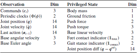
3.2. State and action

States $\boldsymbol{s}_t\in \mathbb{R}^{81}$ are divided into two categories: observations and privileged information. Observations, denoted as $\boldsymbol{o}_t \in \mathbb{R}^{53}$ , consist of data directly obtainable from the user and the robot, including the user commands $\boldsymbol{c}_t\in \mathbb{R}^3$ , periodic clocks $\Phi (\phi )=[sin(\phi ),\ cos(\phi )]^T\in \mathbb{R}^2$ , and onboard sensor data. Privileged information, represented by $\boldsymbol{p}_t \in \mathbb{R}^{28}$ , includes data that is challenging to obtain or prone to significant noise. It is worth noting that no noise is introduced into the critic network to preserve its guiding role and facilitate stable learning during training. Instead, appropriate random noise and time delays are applied to the dual historical observations to enhance the robustness of the actor policy. Table II lists the observations and privileged information in the state space.

Table I. Network architecture for the actor-critic, encoder, and state estimator networks. The configuration of the 1D encoder CNN’s hidden layers is defined as [kernel size, filter size, stride size].

Convolutional Neural Networks (CNN), Multi-Layer Perceptron (MLP).

Table II. Composition of the state space.

The action $\boldsymbol{a}_t \in \mathbb{R}^{14}$ represents the desired joint positions, encompassing both the leg joints and the arm shoulder-pitch joints. A joint-level PD controller subsequently computes the motor torques based on the smoothed action using a low-pass filter (LPF). The policy operates at 100 Hz, while the PD controller runs at 1 kHz.

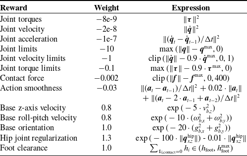
3.3. Reward

We formulate the reward structure to enforce specific gait locomotion while ensuring stability and adaptability. Given that gait and trajectory guidance are derived from the generator in Section 2.2, we introduce tailored reward terms to incorporate prior knowledge. The overall reward function is formulated as:

(9) \begin{equation} \begin{aligned} r=r_{\text{command}} + r_{\text{gait}} + r_{\text{regularization}} \end{aligned} \end{equation}

where $r_{\text{command}}$ denotes the reward for tracking external commands, and the term $r_{\text{gait}}$ ensures adherence to the structured locomotion gait. Additionally, to suppress undesirable motions, a set of regularization rewards $r_{\text{regularization}}$ is introduced to assist smooth and stable action.

3.3.1. Command tracking

Given the desired linear velocity ${v}^d_{x},{v}^d_{x}$ , angular velocity ${\omega }^d_{z}$ , and the base height $h^d_{b}$ , the tracking rewards are defined as:

(10) \begin{equation} \begin{aligned} r_{\text{linear}}&=3\cdot \exp (\!-8\cdot \lVert v^d_{x,y}-v_{x,y}\rVert ^2) \\[5pt] r_{\text{angular}}&=1.5\cdot \exp (\!-8\cdot \lVert \omega ^d_{z}-\omega _{z}\lVert ^2) \\[5pt] r_{\text{height}}&=0.2\cdot \exp (\!-100\cdot \lVert h^d_{b}-h_{b}\lVert ) \end{aligned} \end{equation}

To ensure the robot follows the commanded velocity while avoiding excessive deviations, we define a speed tracking reward $ r_{\text{speed}}$ . Specifically, we penalize low speeds when the robot moves significantly slower than the commanded velocity, assign a neutral reward for excessive speeds, and provide a positive reward when the speed falls within the desired range. Furthermore, since moving in the wrong direction severely affects task performance, we impose a higher penalty for sign mismatches between the actual and commanded velocities. The reward function is defined as:

(11) \begin{equation} r_{\text{speed}} = \begin{cases} -1.0, & \text{if } |{v}_x| \lt 0.5 \cdot |{v}^d_{x}| \\[4pt] 0.0, & \text{if } |{v}_x| \gt 1.2 \cdot |{v}^d_{x}| \\[4pt] 1.2, & \text{if } 0.5 \cdot |{v}^d_{x}| \leq |{v}_x| \leq 1.2 \cdot |{v}^d_{x}| \\[4pt] -2.0, & \text{if } \text{sign}({v}_x) \neq \text{sign}({v}^d_{x}) \end{cases} \end{equation}

3.3.2. Gait style

The gait reward $ r_{\text{gait}}$ comprises three components. The first term, $ r_{\text{contact}}$ , encourages the foot contact pattern to align with the expected structured gait phase, ensuring stable and coordinated locomotion. The second term, $ r_{\text{swing}}$ , reinforces rewards and penalties for feet in the air phase, i.e., $ \boldsymbol{\unicode{x1D7D9}}_{\text{contact}} = \boldsymbol{0}$ , thereby facilitating diverse and adaptable gait patterns. This reward is crucial for learning more complex gaits, as explained in Section 4.2.2. The third term, $ r_{\text{joint}}$ , promotes adherence to predefined joint trajectories, minimizing unnecessary deviations during the exploration process. Given the gait stance indicator $ \boldsymbol{\unicode{x1D7D9}}_{\text{contact}}$ and the joint reference $ \boldsymbol{q}^{\text{ref}}$ derived in Section 2.2, the overall gait reward is formulated as follows:

(12) \begin{equation} \begin{aligned} r_{\text{gait}} &= 1.0 \cdot \sum _{i=0}^1 r_{\text{i,contact}} + 2.0 \cdot r_{\text{swing}} +2.2\cdot r_{\text{joint}} \\ r_{\text{i,contact}} &= \begin{cases} 1.0, & \text{if } \unicode{x1D7D9}_{\text{i,force}}={\unicode{x1D7D9}}_{\text{i,contact}}\\ -0.4, & \text{if } \unicode{x1D7D9}_{\text{i,force}}\neq {\unicode{x1D7D9}}_{\text{i,contact}}\\ \end{cases} \\ r_{\text{swing}} &= \begin{cases} 1.5, & \text{if } \boldsymbol{\unicode{x1D7D9}}_{\text{force}}=\boldsymbol{\unicode{x1D7D9}}_{\text{contact}}=\textbf{0} \\ -0.8, & \text{if } \boldsymbol{\unicode{x1D7D9}}_{\text{force}} \neq \boldsymbol{\unicode{x1D7D9}}_{\text{contact}}=\textbf{0} \end{cases} \\ r_{\text{joint}} &= \exp (\!-2\cdot \lVert \boldsymbol{q}_{m}-\boldsymbol{q}^{\text{ref}}\rVert ) - 0.2\cdot \lVert \boldsymbol{q}_{m}-\boldsymbol{q}^{\text{ref}}\rVert \end{aligned} \end{equation}

where $ \unicode{x1D7D9}_{i,\text{force}}$ denotes the contact indicator for the $ i$ -th foot in the simulator.

3.3.3. Regularization

To suppress undesirable motions, a set of regularization rewards $r_{\text{regularization}}$ is introduced to penalize excessive joint torque, high velocities, unnecessary angular motion, joint regularization, action smoothness, etc. (see Table III). Most of the reward functions are shaped by referring to [25].

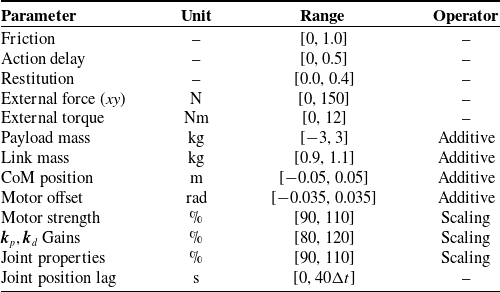
3.4. Domain randomization

Domain randomization is a widely adopted technique in RL to improve policy robustness and reduce the gap between simulation and real-world deployment. In our training details, we apply domain randomization to various physical and control parameters. Specifically, we introduce variations in environment parameters (e.g., friction and restitution), external disturbances (e.g., forces and torques), and dynamic properties of the robot (e.g., payload mass, link mass, and CoM position). Additionally, we randomize actuation characteristics, including motor strength, joint properties, and PD gains, as well as sensory defects such as action delay and joint position lag. These parameters are uniformly sampled from the predefined ranges, as detailed in Table IV.

Table III. Regularization rewards.

Table IV. Domain randomization parameters and their ranges. Additive randomization offsets a parameter within the given range, while scaling applies a multiplicative factor.

4. Experimental results

In this section, we present sim-to-sim evaluations conducted in MuJoCo [26] alongside hardware experiments on the Lingxi-X2 robot. These evaluations measure our method’s performance in terms of speed tracking accuracy, gait cycle stability and consistency, disturbance rejection, and terrain adaptability across different scenarios.

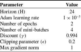
4.1. Setup

We train our policy using the PPO algorithm [27] in the IsaacGym simulator [28], leveraging parallelization across 4096 environments with input normalization. The PPO hyperparameters are provided in Table V. The training process requires approximately 20,000 episodes to achieve a well-performing policy on an Nvidia GeForce 4090 GPU. For a comprehensive evaluation of dynamic locomotion tracking, including stability, disturbance rejection, and adaptability to complex terrain, we compare our approach against the following settings:

• • Baseline [22]: The policy was trained using custom sine waves as the reference trajectory, with the velocity command $\boldsymbol{c}_t=\textbf{0}$ in the gait and trajectory generator set to zero.

• • Asymmetric actor-critic [29]: This method excludes the dual-history window encoding mechanism and uses the same actor and critic observation stack lengths as reported in [29].

• • Model-based method [10, 30]: The controller adopts a cascade scheme, including the nonlinear MPC [30] based on the centroidal dynamics and the WBC [10] based on the full-body dynamics.

• • Ours: The proposed method in this paper.

Additionally, we conduct ablation experiments to assess the contributions of the proposed trajectory generator, gait reward function, upper body motion, and dual-channel network architecture to running performance.

• • Ours w/o reference trajectory: The proposed method without the joint trajectory guidance, i.e., $r_{\text{joint}}=0$ .

• • Ours w/o structured gait : The proposed method without the gait style guidance, i.e., $r_{\text{swing}}=0$ .

• • Ours w/o whole-body control: The proposed method excluding the arm swing control, i.e., $\boldsymbol{a}_t \in \mathbb{R}^{12}$ .

• • Ours w/o long-term history: The proposed method without the 2D-CNN module for extracting the latent representation $\boldsymbol{z}_t$ from long-term observations.

• • Ours w/o short-term history: The proposed method with a single-frame observation instead of the five-frame stack.

Table V. PPO hyperparameters.

All RL-based methods use identical proportional–derivative joint gains, with proportional gains specified as $\boldsymbol{k}_p = 2\cdot [60,\ 60,\ 40,\ 80,\ 40,\ 30,\ 40]^T$ and differential gains as $\boldsymbol{k}_d = 2\cdot [3,\ 3,\ 3,\ 4,\ 2,\ 2,\ 3]^T$ . The joint sequence is ordered left to right, beginning with the left leg and left arm, followed by the right leg and right arm.

4.2. Ablation study

4.2.1. Network architecture

We conducted ablation studies on the dual-history window state encoding by selectively removing each module to evaluate its individual contribution. The results, shown in Figure 5, demonstrate that the proposed method consistently outperforms the ablated variants across all evaluation metrics. In particular, our method achieves faster convergence and higher asymptotic performance in terms of mean reward and episode length (Figure 5, top), reflecting improved learning efficiency and task stability. The gradient-penalized loss, which was not included in the overall PPO objective during ablation experiments, is markedly higher for both ablation variants, with the effect especially pronounced when short-term observations are removed (Figure 5, bottom left). Evaluating this loss separately highlights the stabilizing effect of the dual-history window encoding on policy optimization. Moreover, our full method yields lower base velocity loss than the variant without short-term observations (Figure 5, bottom right), while the removal of long-term observations has little impact. This underscores the critical role of short-term history in accurate velocity estimation. Notably, our method also achieves lower gradient penalty loss compared to the configuration in ref. [29], which adopts a simple asymmetric actor–critic network. Furthermore, their approach lacks the capability to estimate real body velocity. Taken together, these results confirm that both short-term and long-term history windows play essential roles in improving the stability and robustness of the learned locomotion policy.

Figure 5. Ablation study results on the dual-history window state encoding. The plots report the mean reward (top left), episode length (top right), gradient penalty loss (bottom left), and estimated base velocity loss (bottom right). Solid curves represent moving-average filtered data, and shaded regions indicate the standard deviation.

4.2.2. Effect of structured rewards on gait consistency

To evaluate the role of structured gait and trajectory references in maintaining gait consistency, we performed ablation studies on running gaits, which are characterized by a double flight phase. We compared the ground reaction forces (GRFs) of both feet under our proposed method with and without the swing reward $r_{\text{swing}}$ and the reference trajectory reward $r_{\text{joint}}$ . As shown in the top and middle plots of Figure 6, removing $r_{\text{joint}}$ increases apparent alignment with the pre-planned gait schedule, likely due to the increased relative weight of rewards that promote specific motion styles. However, the absence of reference trajectories produces kinematically implausible motions (as illustrated in the supplementary video material), which hinders the learning of robust control policies for highly dynamic tasks such as running. Moreover, excluding $r_{\text{swing}}$ results in mismatched gait sequences (Figure 6, bottom). Although the basic contact reward $r_{\text{contact}}$ remains, it is insufficient to induce a true running gait: the absence of a double flight phase causes the behavior to degenerate into walking. In contrast, our full method achieves a double-hump GRF pattern purely through kinematic motion planning, consistent with the expected behavior in spring–mass dynamics [18].

Figure 6. Ground reaction forces during a $1.3\,{m/s}$ running gait using various method. Solid lines represent low-pass filtered data, while shaded regions indicate data processed with a moving window filter.

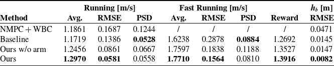
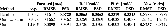
Table VI. Velocity tracking metrics for different gaits.

The bold values indicate that these values outperform others.

4.3. Simulation results

4.3.1. Velocity tracking performance

We evaluate both normal and fast running by starting from rest and ramping to a desired speed and assess tracking performance using the average body height, the average forward velocity, the average velocity tracking reward, the root mean square error (RMSE), and the population standard deviation (PSD) metrics. The results are shown in Figure 7 and Table VI. Given a target speed of $1.3\,{m/s}$ , all methods achieve stable dynamic locomotion, but our method attains the highest average speed and the smallest tracking error. As summarized in Table VI, the maximum achievable speed improves by $9.07\%$ over the baseline. We attribute this gain to the trajectory generator, which supplies reference motions closely aligned with the target speed and thereby guides policy learning, a benefit also reflected in the higher average velocity-tracking reward at convergence.

For a higher target speed of $1.9\,{m/s}$ , the RL-based controller maintains stable locomotion, showing only modest increases in tracking error and body oscillation. In contrast, the model-based controller [10, 30] becomes unstable and often approaches failure (see also the accompanying video). At high running speed, it shows a reduction in body height (Figure 7 middle), a behavior not observed with our policy. These discrepancies reflect an amplified discrepancy between the dynamics model and reality in highly dynamic scenes, which degrades model-based control. Leveraging a neural network’s nonlinear capacity and large-scale interaction data, our RL policy achieves greater locomotion stability and robustness. Furthermore, compared with a policy that ignores arm motions, our approach achieves a lower population standard deviation (PSD) of forward velocity. This indicates reduced body oscillations and improved dynamic stability and highlights the importance of whole-body coordination.

Figure 7. Forward velocity and body height tracking results. Top two rows: RL-based and model-based controllers under a running gait with desired forward speed $v_x^{{d}}=1.3\,{m/s}$ , gait period $T_s=0.66\,{s}$ , and duty factor $\delta =0.65$ . Middle two rows: corresponding body-height variations. Bottom row: RL-based controller under fast running with $v_x^{{d}}=1.9\,{m/s}$ (same $T_s$ and $\delta$ ).

4.3.2. Disturbance rejection capability

The contribution of the structured trajectory generator was evaluated through external force perturbation experiments. As illustrated in Figure 8, disturbances were imposed on the robot torso in eight directions ( $0^\circ -360^\circ$ at $45^\circ$ intervals) and applied for 0.1 $s$ . A trial was considered successful if the robot did not fall, and the maximum resistible external force was evaluated across different methods, thereby demonstrating the role of the trajectory generator in robust running locomotion.

Figure 8. External perturbation evaluation. The left figure shows the maximum external force that each method can resist, while the right figure depicts the directional distribution of perturbations applied during the experiments.

Figure 9 (top) shows snapshots where the robot recovers and maintains stability after external disturbances. Figure 9 (bottom) reports the time histories of forward body velocity, body pitch angle, left–hip joint position, and touchdown phase under a horizontal push of $290\,{N}$ applied at $t=1\,{s}$ . The model-based controller fails under this disturbance, indicating limited disturbance-rejection capability. In contrast, our method and the baseline exhibit comparable immediate responses in terms of forward velocity and body pitch. However, our method achieves faster recovery and requires fewer phase switches than the baseline, as shown in Figure 9 bottom (see also the supplementary video). This improvement can be attributed to the guidance provided by the joint reference reward $r_{\text{joint}}$ during training. Unlike a single sinusoidal reference trajectory, the proposed structured kinematics-based trajectory generator encourages the robot to take larger steps to counter external perturbations, resulting in reactive behaviors more consistent with human locomotion patterns. Figure 8 (left) summarizes a more comprehensive disturbance–rejection evaluation. Compared with the baseline, our method tolerates larger perturbations for forward, backward, and oblique pushes, and it markedly outperforms the classical model-based controller.

Figure 9. Recovery behavior under external perturbations. Top: snapshots of the robot’s recovery after push disturbances using our method. Bottom: responses of forward velocity, body pitch angle, left-hip joint position, and touchdown phase following the perturbation.

4.3.3. Terrain adaptability

We further constructed continuous, complex terrains to evaluate the proposed method’s terrain adaptability relative to the baselines. As illustrated in Figure 10 (top), the environment comprises flat ground, uphill, downhill ( $8^\circ$ ), uneven ground (random height in $[0, 0.05],\mathrm{m}$ ), and transitional terrains. The robot traverses the scene at a target speed of $1.3,\mathrm{m/s}$ . Figure 10 (bottom) shows the time histories of forward velocity, left–hip pitch angle, and body roll angle.

Compared with the other baselines, only our method successfully traversed all terrains. On sloped terrain, RL-based methods exhibited comparable performance. However, on irregular terrain, our method achieved higher dynamic stability and better balance, particularly under uncertain ground height at touchdown (see also the supplementary video). An ablation removing arm coordination produced pronounced body-roll fluctuations and more frequent losses of balance, indicating that upper-body coordination is critical for stable dynamic locomotion. Additionally, in contrast to RL-based methods, the model-based controller performed poorly on slopes and irregular ground because it requires explicit terrain height inputs for landing point selection [1]. Notably, our policy was trained without a terrain curriculum yet remained robust across varying terrains, demonstrating superior adaptability and generalization.

Figure 10. Body behavior on complex terrains. Top: snapshots from the terrain-adaptation experiment using our method. Bottom: time histories of forward body velocity, left-hip joint position, and body roll angle during terrain traversal.

4.4. Hardware results

Terrain setup: The physical experiments were conducted on flat indoor ground with a rigid surface.

Sources of disturbance: During the running trials, an attendant accompanied the robot via a safety tether. However, no external force was exerted on the robot through the tether; it was employed solely as a precautionary measure to safeguard against potential accidents.

Perception system configuration: In contrast to model-based controllers that rely on explicit state estimation, such as extended Kalman filtering, our policy uses only raw proprioceptive signals (joint angles, velocities, and IMU data) as input. This eliminates the need for additional estimation modules, reducing system complexity and improving robustness to modeling errors and sensor noise.

Figure 11. Snapshots of the robot executing running gaits with different methods in the real world.

Figure 12. Base velocity tracking results of different methods in the physical world.

4.4.1. Velocity tracking performance

We evaluated the velocity tracking performance of different methods for running gait control on our real robot. The user specified the desired forward velocity using a handheld controller, and the robot’s snapshots are shown in Figure 11.

As further illustrated in Figure 12 and the accompanying videos, our method achieves superior running performance, characterized by a higher average speed and reduced velocity tracking error. As summarized in Table VII, it improves the maximum speed by 13.36% compared to the approach in ref. [22]. This improvement is attributed to the structured gait trajectories, which are generated based on the desired velocity and enable the exploration of more agile and dynamic running behaviors. We also compared the base velocity fluctuations using different methods. Although our method exhibits a slight increase in the standard deviation of the base’s linear and angular velocities, which is likely due to the higher running speed, the video results show that the overall base stability remains comparable. Importantly, by incorporating coordinated arm motions, our method effectively reduces base posture fluctuations and enhances overall motion stability compared to cases without arm control. As shown at the bottom of Figures 11 and 12, the absence of arm assistance results in considerable yaw fluctuations, increasing the risk of instability and potential falls.

Table VII. Velocity tracking metrics for different gaits.

The bold values indicate that these values outperform others.

4.4.2. Periodic stability

Periodic stability is an important indicator of gait robustness. We evaluate it empirically by analyzing joint limit cycles in the running gait. Figure 13 shows the joint limit cycles obtained from real-world experiments under different methods. Although discrepancies between simulation and reality prevent the trajectories from perfectly matching their simulated counterparts, all methods still form relatively closed limit cycles, suggesting that stable periodic patterns are achieved. Our method demonstrates gait stability comparable to the baseline, and both clearly outperform the variant without arm coordination. The latter exhibits more pronounced oscillations in the joint limit cycles – particularly in the right knee – indicating reduced motion consistency and stability.

Figure 13. Limit cycle of the learned policy of running gaits.

4.5. Discussion

Lightweight trajectory generation: As evidenced by Tables VI, VII, and Figure 9, the proposed control architecture benefits from a kinematics-based gait and trajectory generator, yielding reduced velocity-tracking errors and enabling larger stride lengths both during running and under external disturbances. Unlike prior work [6, 19], our method avoids complex model-based trajectory generators and large externally collected datasets. This simple yet effective generator is sufficient to guide the learning of robust and stable running gaits, thereby streamlining the RL pipeline and improving usability. However, unlike the method in ref. [20], our approach may not handle transitions between diverse gaits.

Terrain adaptability: Although our method is not explicitly trained on certain complex terrains, it still demonstrates strong adaptability and generalization to unseen scenarios, outperforming classical model-based methods that rely on detailed terrain information. Nevertheless, the approach may still fail in more challenging environments, for instance, stair climbing.

Whole-body coordination: Our method seamlessly integrates upper-limb motion within a unified control policy, thereby enhancing the dynamic stability and robustness of locomotion. Compared with [31], our method achieves similar humanoid arm motion without resorting to separate multi-agent training for the upper and lower limbs.

5. Conclusion and future work

In this paper, we propose a reinforcement learning framework for robust bipedal running. The framework incorporates a kinematics-based structured gait generator during training, which facilitates efficient policy learning and exploration. To bridge the sim-to-real gap and enable zero-shot transfer, we introduce two auxiliary networks within an asymmetric actor–critic architecture that infer latent environment state and body velocity from long- and short-horizon observation histories. Extensive experiments in simulation and on hardware demonstrate that our method significantly enhances running agility and achieves larger stride lengths, both in free running and under external disturbances. Moreover, the learned gait maintains periodic consistency on slopes and uneven terrain while naturally capturing the ground reaction force characteristics of spring-mass dynamics without explicitly modeling them.

Our future work will focus on a unified control framework that encompasses multiple locomotion gaits and supports seamless transitions among them. Developing a general strategy for diverse bipedal gaits remains challenging and significant.