


1. Introduction
In this note we investigate geometric properties of invariant spatio-temporal random fields $X\colon\mathbb M^d\times \mathbb R\to \mathbb R$
,
$X\colon\mathbb M^d\times \mathbb R\to \mathbb R$
, $(x,t)\mapsto X(x,t)$
defined on compact two-point homogeneous spaces
$(x,t)\mapsto X(x,t)$
defined on compact two-point homogeneous spaces $\mathbb M^d$
in any dimension
$\mathbb M^d$
in any dimension $d\ge 2$
, and evolving over time. A key example is
$d\ge 2$
, and evolving over time. A key example is $\mathbb M^d=\mathbb S^d$
, the d-dimensional sphere with the round metric.
$\mathbb M^d=\mathbb S^d$
, the d-dimensional sphere with the round metric.
In recent decades the theory of spherical random fields, or more generally random fields on Riemannian manifolds, has received growing interest, also in view of possible applications to cosmology, brain imaging, machine learning, and climate science, to cite a few. As for the latter, it is indeed natural to model the Earth surface temperature as a random field on $\mathbb S^2$
evolving over time.
$\mathbb S^2$
evolving over time.
1.1. Previous work on the sphere
In [Reference Caponera, Marinucci and Vidotto2] the authors, relying on this probabilistic model, are able to detect Earth surface temperature anomalies via analysis of climate data collected from 1949 to 2020. On the other hand, in [Reference Marinucci, Rossi and Vidotto23] geometric properties of invariant Gaussian random fields Z on $\mathbb S^2\times \mathbb R$
are investigated (see also [Reference Leonenko and Ruiz-Medina14]). (In this manuscript,
$\mathbb S^2\times \mathbb R$
are investigated (see also [Reference Leonenko and Ruiz-Medina14]). (In this manuscript, $\mathbb N_0=\lbrace 0,1,2,\dots \rbrace$
while
$\mathbb N_0=\lbrace 0,1,2,\dots \rbrace$
while $\mathbb N=\mathbb N_0\setminus \lbrace 0 \rbrace$
.) The Fourier components of Z, say
$\mathbb N=\mathbb N_0\setminus \lbrace 0 \rbrace$
.) The Fourier components of Z, say $\lbrace Z_\ell \rbrace_{\ell\in \mathbb N_0}$
, satisfying
$\lbrace Z_\ell \rbrace_{\ell\in \mathbb N_0}$
, satisfying $\Delta_{\mathbb S^2} Z_\ell(\cdot, t) + \ell(\ell+1) Z_\ell(\cdot, t)=0$
(where
$\Delta_{\mathbb S^2} Z_\ell(\cdot, t) + \ell(\ell+1) Z_\ell(\cdot, t)=0$
(where $\Delta_{\mathbb S^2}$
is the Laplace–Beltrami operator on the sphere) are allowed to have short or long memory in time (independently of one another), i.e. an integrable or non-integrable temporal covariance function. The parametric model is related to functions that at infinity behave like
$\Delta_{\mathbb S^2}$
is the Laplace–Beltrami operator on the sphere) are allowed to have short or long memory in time (independently of one another), i.e. an integrable or non-integrable temporal covariance function. The parametric model is related to functions that at infinity behave like $t^{-2}$
(or any other integrable power) in the short-memory case, and
$t^{-2}$
(or any other integrable power) in the short-memory case, and $t^{-\beta_\ell}$
in the long-memory case, where
$t^{-\beta_\ell}$
in the long-memory case, where $\beta_\ell\in (0,1)$
. In order to make the notation more compact, the short-memory case is associated with
$\beta_\ell\in (0,1)$
. In order to make the notation more compact, the short-memory case is associated with $\beta_\ell=1$
, representing an integrable power law at infinity. For details, see (10) and Assumption 1.
$\beta_\ell=1$
, representing an integrable power law at infinity. For details, see (10) and Assumption 1.
In particular, in [Reference Marinucci, Rossi and Vidotto23] the authors focus on the large-time (as $T\to +\infty$
) fluctuations of the average empirical area
$T\to +\infty$
) fluctuations of the average empirical area
 \begin{equation} \mathcal M^Z_T(u) \,:\!=\, \int_{[0,T]}\int_{\mathbb S^2}(\mathbf{1}_{\lbrace Z(x,t)\ge u\rbrace} - \mathbb P(Z(x,t)\ge u))\,{\mathrm{d}} x\,{\mathrm{d}} t,\end{equation}
where $u\in \mathbb R$
is the threshold at which we ‘cut’ the field. Note that in (1) the spatial domain is fixed.
$u\in \mathbb R$
is the threshold at which we ‘cut’ the field. Note that in (1) the spatial domain is fixed.
Both first- and second-order fluctuations of $\mathcal M_T^Z(u)$
depend on a subtle interplay between the parameters of the model, in particular between
$\mathcal M_T^Z(u)$
depend on a subtle interplay between the parameters of the model, in particular between
 \begin{equation} \beta_{\ell^*} \,:\!=\, \min_{\ell\in \mathbb N} \beta_\ell\end{equation}
(which the authors of [Reference Marinucci, Rossi and Vidotto23] assume exists), the value of $\beta_0$
, and the threshold u. The core of their proofs relies on the decomposition of (1) into so-called Wiener chaoses: basically, when Z has zero mean and unit variance,
$\beta_0$
, and the threshold u. The core of their proofs relies on the decomposition of (1) into so-called Wiener chaoses: basically, when Z has zero mean and unit variance, $\mathcal M_T^Z(u)$
can be written as an orthogonal series in
$\mathcal M_T^Z(u)$
can be written as an orthogonal series in $L^2(\Omega)$
of the form
$L^2(\Omega)$
of the form
 \begin{equation} \mathcal M_T^Z(u) = \sum_{q=1}^{+\infty}\mathcal M_T^Z(u)[q] = \sum_{q=1}^{+\infty}\int_{[0,T]}\bigg(\frac{\phi(u)H_{q-1}(u)}{q!}\int_{\mathbb S^2}H_q(Z(x,t))\,{\mathrm{d}} x\bigg)\,{\mathrm{d}} t,\end{equation}
where $\lbrace H_q\rbrace_{q\in \mathbb N_0}$
represents the family of Hermite polynomials, and
$\lbrace H_q\rbrace_{q\in \mathbb N_0}$
represents the family of Hermite polynomials, and $\phi$
the standard Gaussian density. This expansion is satisfied by any
$\phi$
the standard Gaussian density. This expansion is satisfied by any $L^2(\Omega)$
-functional of a Gaussian field, and it is based on the fact that Hermite polynomials form a complete orthogonal basis for the space of square-integrable functions on the real line with respect to the Gaussian measure.
$L^2(\Omega)$
-functional of a Gaussian field, and it is based on the fact that Hermite polynomials form a complete orthogonal basis for the space of square-integrable functions on the real line with respect to the Gaussian measure.
The quantity $\beta_0\in (0,1]$
is the memory parameter of the temporal part of
$\beta_0\in (0,1]$
is the memory parameter of the temporal part of $\mathcal M_T^Z(u)[1]$
in (3), i.e. of the stochastic process
$\mathcal M_T^Z(u)[1]$
in (3), i.e. of the stochastic process $\mathbb R\ni t\mapsto \phi(u) \int_{\mathbb S^2} Z(x,t)\,{\mathrm{d}} x$
. If
$\mathbb R\ni t\mapsto \phi(u) \int_{\mathbb S^2} Z(x,t)\,{\mathrm{d}} x$
. If $\beta_0=1$
, then the asymptotic variance of
$\beta_0=1$
, then the asymptotic variance of $\mathcal M_T^Z(u)[1]$
is of order T, otherwise it is of order
$\mathcal M_T^Z(u)[1]$
is of order T, otherwise it is of order $T^{2-\beta_0}$
. Of course,
$T^{2-\beta_0}$
. Of course, $\mathcal M_T^Z(u)[1]$
is Gaussian for every
$\mathcal M_T^Z(u)[1]$
is Gaussian for every $T>0$
.
$T>0$
.
As for the second chaotic component, it is worth noticing that it vanishes if and only if $u=0$
(indeed,
$u=0$
(indeed, $H_1(u)=u$
); for
$H_1(u)=u$
); for $u\ne 0$
, roughly speaking, the dependence property of its integrand stochastic process relies on the interplay between
$u\ne 0$
, roughly speaking, the dependence property of its integrand stochastic process relies on the interplay between $\beta_{\ell^*}$
and
$\beta_{\ell^*}$
and $\beta_0$
: if
$\beta_0$
: if $2\beta_{\ell^*} < \min(1, 2\beta_0)$
then the asymptotic variance of
$2\beta_{\ell^*} < \min(1, 2\beta_0)$
then the asymptotic variance of $\mathcal M_T^Z(u)[2]$
is of order
$\mathcal M_T^Z(u)[2]$
is of order $T^{2-2\beta_{\ell^*}}$
, while if both
$T^{2-2\beta_{\ell^*}}$
, while if both $2\beta_{\ell^*}$
and
$2\beta_{\ell^*}$
and $2\beta_0$
are
$2\beta_0$
are $>1$
it is of order T. In the former case, the limiting distribution of
$>1$
it is of order T. In the former case, the limiting distribution of $\mathcal M_T^Z(u)[2]$
after standardization is non-Gaussian, in the latter case a central limit theorem holds. The analysis of higher-order chaotic components of (3) is somewhat analogous.
$\mathcal M_T^Z(u)[2]$
after standardization is non-Gaussian, in the latter case a central limit theorem holds. The analysis of higher-order chaotic components of (3) is somewhat analogous.
In particular, in the ‘short-memory case’ (that corresponds to $\beta_0=1$
and
$\beta_0=1$
and $\beta_{\ell^*}=\min_{\ell\in \mathbb N} \beta_\ell$
such that
$\beta_{\ell^*}=\min_{\ell\in \mathbb N} \beta_\ell$
such that $\beta_{\ell^*}> \frac12$
for
$\beta_{\ell^*}> \frac12$
for $u\ne 0$
or
$u\ne 0$
or $\beta_{\ell^*}> \frac13$
for
$\beta_{\ell^*}> \frac13$
for $u=0$
) the statistic in (1), once divided by
$u=0$
) the statistic in (1), once divided by $\sqrt T$
, shows Gaussian fluctuations. Indeed, each non-null chaotic component in (3) has an asymptotic variance of order T (so the whole variance series is of order T), and once divided by
$\sqrt T$
, shows Gaussian fluctuations. Indeed, each non-null chaotic component in (3) has an asymptotic variance of order T (so the whole variance series is of order T), and once divided by $\sqrt{T}$
, converges to a Gaussian random variable (r.v.) via an application of the fourth moment theorem (hence, thanks to a Breuer–Major argument, for
$\sqrt{T}$
, converges to a Gaussian random variable (r.v.) via an application of the fourth moment theorem (hence, thanks to a Breuer–Major argument, for $\mathcal M_T^Z(u)/\sqrt T$
a central limit theorem holds [Reference Nourdin and Peccati26, Theorem 6.3.1]).
$\mathcal M_T^Z(u)/\sqrt T$
a central limit theorem holds [Reference Nourdin and Peccati26, Theorem 6.3.1]).
In the ‘long-memory case’, in particular when $2\beta_{\ell^*} < \min(1,\beta_0)$
, for
$2\beta_{\ell^*} < \min(1,\beta_0)$
, for $u\ne 0$
the statistics
$u\ne 0$
the statistics $\mathcal M_T^Z(u)$
and
$\mathcal M_T^Z(u)$
and $\mathcal M_T^Z(u)[2]$
are asymptotically equivalent in
$\mathcal M_T^Z(u)[2]$
are asymptotically equivalent in $L^2(\Omega)$
, and
$L^2(\Omega)$
, and $\mathcal M_T^Z(u)[2]$
converges in distribution towards a linear combination of independent Rosenblatt r.v.s, once divided by
$\mathcal M_T^Z(u)[2]$
converges in distribution towards a linear combination of independent Rosenblatt r.v.s, once divided by $T^{1-\beta_{\ell^*}}$
(hence (1) does not have Gaussian fluctuations). This non-central limit theorem follows from standard results for Hermite rank-two functionals of Gaussian fields in the presence of long memory [Reference Dobrushin and Major5, Reference Taqqu31].
$T^{1-\beta_{\ell^*}}$
(hence (1) does not have Gaussian fluctuations). This non-central limit theorem follows from standard results for Hermite rank-two functionals of Gaussian fields in the presence of long memory [Reference Dobrushin and Major5, Reference Taqqu31].
1.2. Our main contribution
The aim of the present note is to take a first step towards possible natural generalizations in two directions of the results of [Reference Marinucci, Rossi and Vidotto23] mentioned in Section 1.1: the type of randomness of the field and the underlying manifold. Indeed, as briefly anticipated, we want to study the large-time behavior of the statistic $\mathcal M_T^X(u)$
defined as in (1) with the spherical random field Z replaced by an invariant time-dependent chi-squared distributed process X on a two-point homogeneous space
$\mathcal M_T^X(u)$
defined as in (1) with the spherical random field Z replaced by an invariant time-dependent chi-squared distributed process X on a two-point homogeneous space $\mathbb M^d$
in any dimension
$\mathbb M^d$
in any dimension $d\ge 2$
(see Definition 1). Of course, we consider only the case of positive thresholds, i.e.
$d\ge 2$
(see Definition 1). Of course, we consider only the case of positive thresholds, i.e. $u>0$
. (For
$u>0$
. (For $u=0$
, it is natural to study the time behavior of the set
$u=0$
, it is natural to study the time behavior of the set $\lbrace X(\cdot , t) =0\rbrace$
. We leave this as a topic for future research – see [Reference Marinucci, Rossi and Vidotto24] for fluctuations of the level lines of a spatio-temporal Gaussian field on the 2-sphere.)
$\lbrace X(\cdot , t) =0\rbrace$
. We leave this as a topic for future research – see [Reference Marinucci, Rossi and Vidotto24] for fluctuations of the level lines of a spatio-temporal Gaussian field on the 2-sphere.)
To be more precise, the marginal law of $X=X_k$
is a chi-square distribution with
$X=X_k$
is a chi-square distribution with $k\in \mathbb N$
degrees of freedom. In order to define
$k\in \mathbb N$
degrees of freedom. In order to define $X_k$
, it suffices to consider k independent and identically distributed (i.i.d.) copies
$X_k$
, it suffices to consider k independent and identically distributed (i.i.d.) copies $Z_1,\dots, Z_k$
of an invariant Gaussian random field Z on
$Z_1,\dots, Z_k$
of an invariant Gaussian random field Z on $\mathbb M^d\times \mathbb R$
(generalizing the definition for
$\mathbb M^d\times \mathbb R$
(generalizing the definition for $\mathbb S^2\times \mathbb R$
) with standard Gaussian marginals, and take the sum of their squares,
$\mathbb S^2\times \mathbb R$
) with standard Gaussian marginals, and take the sum of their squares, $X_k(x,t)=Z_1(x,t)^2 +\dots + Z_k(x,t)^2$
,
$X_k(x,t)=Z_1(x,t)^2 +\dots + Z_k(x,t)^2$
, $(x,t)\in \mathbb M^d\times \mathbb R$
. Our main results mirror those obtained for the statistic in (1) in the spherical case. It is worth stressing that although our proofs closely follow the strategy developed in [Reference Marinucci, Rossi and Vidotto23], there are a few differences and we obtain some novel results that may be of independent interest. First of all, it is possible to obtain a chaotic expansion similar to (3) for
$(x,t)\in \mathbb M^d\times \mathbb R$
. Our main results mirror those obtained for the statistic in (1) in the spherical case. It is worth stressing that although our proofs closely follow the strategy developed in [Reference Marinucci, Rossi and Vidotto23], there are a few differences and we obtain some novel results that may be of independent interest. First of all, it is possible to obtain a chaotic expansion similar to (3) for $\mathcal M_T^{X_k}(u)$
, actually the distribution of the underlying noise
$\mathcal M_T^{X_k}(u)$
, actually the distribution of the underlying noise $(Z_1,\dots, Z_k)$
is Gaussian. Due to parity of the involved functions, terms of odd order q vanish, and this expansion can hence be rewritten in terms of Laguerre polynomials. We find along the way an explicit formula for chaotic coefficients of the function
$(Z_1,\dots, Z_k)$
is Gaussian. Due to parity of the involved functions, terms of odd order q vanish, and this expansion can hence be rewritten in terms of Laguerre polynomials. We find along the way an explicit formula for chaotic coefficients of the function $\mathbf{1}_{\lbrace \chi^2(k)\ge u\rbrace}$
for
$\mathbf{1}_{\lbrace \chi^2(k)\ge u\rbrace}$
for $u>0$
, a result that may have some independent interest. (Here and in what follows,
$u>0$
, a result that may have some independent interest. (Here and in what follows, $\chi^2(k)$
denotes a chi-square r.v. with k degrees of freedom.)
$\chi^2(k)$
denotes a chi-square r.v. with k degrees of freedom.)
Let us define $\beta_{\ell^*}\,:\!=\,\min_{\ell\in \mathbb N_0}\beta_\ell$
– see also (2). As for the asymptotic variance and limiting distribution of
$\beta_{\ell^*}\,:\!=\,\min_{\ell\in \mathbb N_0}\beta_\ell$
– see also (2). As for the asymptotic variance and limiting distribution of $\mathcal M_T^{X_k}(u)$
, for
$\mathcal M_T^{X_k}(u)$
, for $\beta_{\ell^*} > \frac12$
it is of order T and a central limit theorem holds for every
$\beta_{\ell^*} > \frac12$
it is of order T and a central limit theorem holds for every $u>0$
, while for
$u>0$
, while for $\beta_{\ell^*} < \frac12$
it is of order
$\beta_{\ell^*} < \frac12$
it is of order $T^{2-2\beta_{\ell^*}}$
and convergence to a linear combination of independent Rosenblatt r.v.s holds (still for every
$T^{2-2\beta_{\ell^*}}$
and convergence to a linear combination of independent Rosenblatt r.v.s holds (still for every $u>0$
).
$u>0$
).
1.3. Brief overview of the literature
The existing literature is rich in results on sojourn times of random fields, and more generally on the geometry of their excursion sets. As for chi-square random fields on manifolds, it is worth mentioning as a possible application in astrophysics in the analysis of the cosmic microwave background (CMB) data. Indeed, the CMB polarization intensity is modeled as a spin-2 spherical random field [Reference Marinucci and Peccati21, Chapter 12] and, as noted in [Reference Carones, Carrón Duque, Marinucci, Migliaccio and Vittorio3], the expected Lipschitz–Killing curvatures of corresponding excursion sets coincide with those of a chi-square random field on the sphere. In this regard, recently in [Reference Marinucci and Stecconi25] critical points of chi-square random fields on manifolds have been investigated. In the Euclidean setting the distribution of sojourn functionals for spatio-temporal Gaussian random fields with long memory has been studied in [Reference Leonenko and Ruiz-Medina14], while in [Reference Leonenko, Ruiz-Medina and Taqqu15] the case of nonlinear functionals of Gamma-correlated random fields with long memory (and no time dependence) has been treated by means of Laguerre chaos. See also [Reference Makogin and Spodarev20] for limit theorems in the case of subordinated Gaussian random fields, still with long-range dependence. The paper [Reference Leonenko, Maini, Nourdin and Pistolato12] contains recent developments on this subject; indeed, the authors investigate limit theorems for p-domain functionals of stationary Gaussian fields. Moreover, in [Reference Dębicki, Hashorva, Liu and Michna4] the authors show that under a very general framework there is an interesting relationship between tail asymptotics of sojourn times and that of the supremum of the random field. To conclude, let us recall that the decomposition structure of (time-varying) Gaussian random fields on compact two-point homogeneous spaces was studied, e.g., in [Reference Ma and Malyarenko19]; see also [Reference Lu, Ma and Xiao18] for regularity properties of their sample paths. Of course, this list is by no means complete.
2. Background and notation
Let $\mathbb M^d$
be a two-point homogeneous compact Riemannian manifold with dimension
$\mathbb M^d$
be a two-point homogeneous compact Riemannian manifold with dimension $d\ge 2$
, and denote by
$d\ge 2$
, and denote by $\rho$
its geodesic distance. Here we assume that
$\rho$
its geodesic distance. Here we assume that $\rho(x,y) \in [0,\pi]$
for every
$\rho(x,y) \in [0,\pi]$
for every $x,y \in \mathbb{M}^d$
, and consider also a normalized Riemannian measure, denoted by
$x,y \in \mathbb{M}^d$
, and consider also a normalized Riemannian measure, denoted by ${\mathrm{d}}\nu$
, so that
${\mathrm{d}}\nu$
, so that $\int_{\mathbb{M}^d} {\mathrm{d}}\nu = 1$
. Denoting by G the group of isometries of
$\int_{\mathbb{M}^d} {\mathrm{d}}\nu = 1$
. Denoting by G the group of isometries of $\mathbb M^d$
, for any set of four points
$\mathbb M^d$
, for any set of four points $x_1, y_1, x_2, y_2\in \mathbb M^d$
with
$x_1, y_1, x_2, y_2\in \mathbb M^d$
with $\rho(x_1, y_1)=\rho(x_2, y_2)$
, there exists
$\rho(x_1, y_1)=\rho(x_2, y_2)$
, there exists $\varphi \in G$
such that
$\varphi \in G$
such that $\varphi(x_1)=x_2$
and
$\varphi(x_1)=x_2$
and $\varphi(y_1)=y_2$
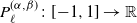
. As pointed out in [Reference Wang32],
$\varphi(y_1)=y_2$
. As pointed out in [Reference Wang32], $\mathbb M^d$
belongs to one of the following categories: the unit (hyper)sphere
$\mathbb M^d$
belongs to one of the following categories: the unit (hyper)sphere $\mathbb S^d$
,
$\mathbb S^d$
, $d=2,3,\dots$
; the real projective spaces
$d=2,3,\dots$
; the real projective spaces $\mathbb P^d(\mathbb R)$
,
$\mathbb P^d(\mathbb R)$
, $d=2,3,\dots$
; the complex projective spaces
$d=2,3,\dots$
; the complex projective spaces $\mathbb P^d(\mathbb C)$
,
$\mathbb P^d(\mathbb C)$
, $d=4,6,\dots$
; the quaternionic projective spaces
$d=4,6,\dots$
; the quaternionic projective spaces $\mathbb P^d(\mathbb H)$
,
$\mathbb P^d(\mathbb H)$
, $d = 8, 12, \dots$
; and the Cayley projective plane
$d = 8, 12, \dots$
; and the Cayley projective plane $\mathbb P^d(\mathrm{Cay})$
,
$\mathbb P^d(\mathrm{Cay})$
, $d = 16$
.
$d = 16$
.
2.1. Fourier analysis for two-point homogeneous spaces
Let $\Delta_{\mathbb{M}^d}$
be the Laplace–Beltrami operator on
$\Delta_{\mathbb{M}^d}$
be the Laplace–Beltrami operator on $\mathbb{M}^d$
(see, e.g., [Reference Giné Masdéu6, Reference Helgason7, Reference Ma and Malyarenko19]). It is well known that the spectrum of
$\mathbb{M}^d$
(see, e.g., [Reference Giné Masdéu6, Reference Helgason7, Reference Ma and Malyarenko19]). It is well known that the spectrum of $\Delta_{\mathbb{M}^d}$
is purely discrete, the eigenvalues being
$\Delta_{\mathbb{M}^d}$
is purely discrete, the eigenvalues being $\lambda_\ell = \lambda_\ell(\mathbb{M}^d) = -\ell(\ell+\alpha+\beta+1)$
,
$\lambda_\ell = \lambda_\ell(\mathbb{M}^d) = -\ell(\ell+\alpha+\beta+1)$
, $\ell \in \Lambda$
, where
$\ell \in \Lambda$
, where
 \begin{equation} \Lambda = \Lambda(\mathbb{M}^d) = \begin{cases} \{n \in \mathbb{N}_0\colon n\text{ even}\} & \text{if } \mathbb{M}^d = \mathbb{P}^d(\mathbb R), \\ \mathbb{N}_0 & \text{if } \mathbb{M}^d \ne \mathbb{P}^d(\mathbb R), \end{cases}\end{equation}
and the parameters $\alpha, \beta$
are reported in Table 1. Now consider
$\alpha, \beta$
are reported in Table 1. Now consider $L^2(\mathbb{M}^d)$
, the space of real-valued, square-integrable functions on
$L^2(\mathbb{M}^d)$
, the space of real-valued, square-integrable functions on $\mathbb{M}^d$
with respect to the normalized Riemannian measure
$\mathbb{M}^d$
with respect to the normalized Riemannian measure ${\mathrm{d}}\nu$
, endowed with the standard inner product
${\mathrm{d}}\nu$
, endowed with the standard inner product $\langle \cdot, \cdot \rangle_{L^2(\mathbb M^d)}$
.
$\langle \cdot, \cdot \rangle_{L^2(\mathbb M^d)}$
.
(Recall the definition of the set $\Lambda$
in (4).) For every
$\Lambda$
in (4).) For every $\ell \in \Lambda$
, eigenfunctions corresponding to the same eigenvalue
$\ell \in \Lambda$
, eigenfunctions corresponding to the same eigenvalue $\lambda_\ell$
form a finite-dimensional vector space, denoted by
$\lambda_\ell$
form a finite-dimensional vector space, denoted by $\mathcal{Y}_\ell = \mathcal{Y}_\ell (\mathbb{M}^d)$
, with dimension
$\mathcal{Y}_\ell = \mathcal{Y}_\ell (\mathbb{M}^d)$
, with dimension
 \begin{equation*} \operatorname{dim}(\mathcal{Y}_\ell) = \frac{(2\ell + \alpha + \beta + 1) \Gamma(\beta +1) \Gamma(\ell +\alpha + \beta +1)\Gamma(\ell +\alpha +1)} {\Gamma(\alpha +1) \Gamma(\alpha + \beta +2)\Gamma(\ell +1)\Gamma(\ell +\beta+1)}.\end{equation*}
It is well known that $L^2(\mathbb M^d) = \bigoplus_{\ell \in \Lambda} \mathcal{Y}_\ell$
, where
$L^2(\mathbb M^d) = \bigoplus_{\ell \in \Lambda} \mathcal{Y}_\ell$
, where $\bigoplus$
stands for the orthogonal sum, in
$\bigoplus$
stands for the orthogonal sum, in $L^2$
, of vector spaces. Moreover, given a real-valued orthonormal basis of
$L^2$
, of vector spaces. Moreover, given a real-valued orthonormal basis of $\mathcal{Y}_\ell$
, say
$\mathcal{Y}_\ell$
, say $\{ Y_{\ell,m}, m=1,\dots, \operatorname{dim}(\mathcal{Y}_\ell) \}$
, any function
$\{ Y_{\ell,m}, m=1,\dots, \operatorname{dim}(\mathcal{Y}_\ell) \}$
, any function $f \in L^2(\mathbb{M}^d)$
can be written as a series, converging in
$f \in L^2(\mathbb{M}^d)$
can be written as a series, converging in $L^2$
, of the form
$L^2$
, of the form
 \begin{equation*} f = \sum_{\ell\in\Lambda}\sum_{m=1}^{\operatorname{dim}(\mathcal{Y}_\ell)}\langle f,Y_{\ell,m}\rangle_{L^2(\mathbb{M}^d)}Y_{\ell,m}.\end{equation*}
Table 1. Eigenvalue parameters $\alpha$
and
$\alpha$
and $\beta$
.
$\beta$
.

From [Reference Giné Masdéu6, Theorem 3.2] an addition formula holds: for any $\ell \in \Lambda$
,
$\ell \in \Lambda$
,
 \begin{equation} \frac{1}{\operatorname{dim}(\mathcal{Y}_\ell)}\sum_{m=1}^{\operatorname{dim}(\mathcal{Y}_\ell)}Y_{\ell,m}(x)Y_{\ell,m}(y) = \frac{P_{\ell }^{(\alpha, \beta)}(\cos \varepsilon \rho(x,y))}{P_{\ell}^{(\alpha, \beta)}(1)},\end{equation}
where $\varepsilon=\frac12$
if
$\varepsilon=\frac12$
if $\mathbb{M}^d = \mathbb{P}^d(\mathbb R)$
and
$\mathbb{M}^d = \mathbb{P}^d(\mathbb R)$
and $\varepsilon=1$
otherwise. The functions
$\varepsilon=1$
otherwise. The functions $P_{\ell}^{(\alpha,\beta)}\colon[\!-\!1,1]\to\mathbb{R}$
,
$P_{\ell}^{(\alpha,\beta)}\colon[\!-\!1,1]\to\mathbb{R}$
, $\ell \in \mathbb{N}_0$
, are the well-known Jacobi polynomials [Reference Szegö29]. Notably, when
$\ell \in \mathbb{N}_0$
, are the well-known Jacobi polynomials [Reference Szegö29]. Notably, when $\mathbb{M}^d = \mathbb{S}^2$
(the unit two-dimensional sphere with the round metric), they reduce to the Legendre polynomials
$\mathbb{M}^d = \mathbb{S}^2$
(the unit two-dimensional sphere with the round metric), they reduce to the Legendre polynomials $P_\ell$
,
$P_\ell$
, $\ell \in \mathbb N_0$
. Recall that
$\ell \in \mathbb N_0$
. Recall that
 \begin{equation*} P_{\ell}^{(\alpha, \beta)}(1) =\binom{\ell +\alpha}{\ell},\end{equation*}
and that $|P_{\ell}^{(\alpha, \beta)}(z)| \le P_{\ell}^{(\alpha, \beta)}(1)$
,
$|P_{\ell}^{(\alpha, \beta)}(z)| \le P_{\ell}^{(\alpha, \beta)}(1)$
, $z \in [\!-\!1,1]$
.
$z \in [\!-\!1,1]$
.
In general, the reason for the ‘exceptional’ behavior of the real projective spaces is discussed, for instance, in [Reference Kushpel10] (see also [Reference Kushpel and Tozoni11] and the references therein).
2.2. Spatio-temporal invariant random fields
Consider a mean-square continuous isotropic and stationary centered Gaussian field Z on $\mathbb M^d\times \mathbb R$
, that is, a measurable map
$\mathbb M^d\times \mathbb R$
, that is, a measurable map $Z\colon\Omega \times \mathbb M^d\times \mathbb R\to \mathbb R$
, where
$Z\colon\Omega \times \mathbb M^d\times \mathbb R\to \mathbb R$
, where $(\Omega, \mathcal F, \mathbb P)$
is some probability space, such that:
$(\Omega, \mathcal F, \mathbb P)$
is some probability space, such that:
-
• $(Z(x_1, t_1),\dots, Z(x_n, t_n))$
is Gaussian for every n and every
$x_1,\dots,x_n\in\mathbb M^d$
,
$t_1,\dots,t_n\in \mathbb R$
;
$(Z(x_1, t_1),\dots, Z(x_n, t_n))$
is Gaussian for every n and every
$x_1,\dots,x_n\in\mathbb M^d$
,
$t_1,\dots,t_n\in \mathbb R$
; -
•
$\mathbb E[Z(x,t)]=0$
for every
$x\in \mathbb M^d$
,
$t\in \mathbb R$
; -
• there exists a function
$\Sigma\colon[0,\pi]\times \mathbb R\to \mathbb R$
such that, for every
$x,y\in \mathbb M^d$
,
$t,s\in \mathbb R$
,
$\mathbb E[Z(x,t)Z(y,s)] = \Sigma(\rho(x,y), t-s)$
– see also [Reference Ma and Malyarenko19, Definition 1]; -
•
$\Sigma$
is a continuous function.


It is well known [Reference Ma and Malyarenko19, Theorem 3/Corollary 1] that, under these assumptions, $\Sigma$
admits the spectral decomposition
$\Sigma$
admits the spectral decomposition
 \begin{equation} \Sigma(\theta,\tau) = \sum_{\ell\in\Lambda}\kappa_\ell C_\ell(\tau)P^{(\alpha,\beta)}_{\ell}(\cos\varepsilon\theta), \quad \tau\in \mathbb R, \theta\in [0,\pi],\end{equation}
where $\kappa_\ell = {\operatorname{dim}(\mathcal{Y}_\ell)}/{P_{\ell}^{(\alpha, \beta)}(1)}$
,
$\kappa_\ell = {\operatorname{dim}(\mathcal{Y}_\ell)}/{P_{\ell}^{(\alpha, \beta)}(1)}$
, $\varepsilon=\frac12$
if
$\varepsilon=\frac12$
if $\mathbb{M}^d = \mathbb{P}^d(\mathbb R)$
and
$\mathbb{M}^d = \mathbb{P}^d(\mathbb R)$
and $\varepsilon=1$
otherwise; the series on the right-hand side (r.h.s.) of (6) converges uniformly on
$\varepsilon=1$
otherwise; the series on the right-hand side (r.h.s.) of (6) converges uniformly on $[0,\pi]\times \mathbb R$
, and
$[0,\pi]\times \mathbb R$
, and $C_\ell\colon\mathbb R\to \mathbb R$
,
$C_\ell\colon\mathbb R\to \mathbb R$
, $\ell\in \Lambda$
, are semi-positive-definite functions. Note that the uniform convergence of the series in (6) is equivalent to the condition
$\ell\in \Lambda$
, are semi-positive-definite functions. Note that the uniform convergence of the series in (6) is equivalent to the condition $\sum_{\ell\in \Lambda} \operatorname{dim}(\mathcal{Y}_\ell) C_\ell(0) <+\infty$
.
$\sum_{\ell\in \Lambda} \operatorname{dim}(\mathcal{Y}_\ell) C_\ell(0) <+\infty$
.
Throughout this work we assume that the field Z has unit variance:
 \begin{equation} \Sigma(0,0) = \sum_{\ell\in \Lambda} \operatorname{dim}(\mathcal{Y}_\ell) C_\ell(0) = 1.\end{equation}
Definition 1. Let $Z_1, Z_2,\dots, Z_k$
be
$Z_1, Z_2,\dots, Z_k$
be $k\in \mathbb N$
i.i.d. copies of an isotropic and stationary centered unit-variance Gaussian field Z on
$k\in \mathbb N$
i.i.d. copies of an isotropic and stationary centered unit-variance Gaussian field Z on $\mathbb M^d\times \mathbb R$
For
$\mathbb M^d\times \mathbb R$
For $k\in \mathbb N$
, we define the spatio-temporal
$k\in \mathbb N$
, we define the spatio-temporal $\chi^2(k)$
-random field
$\chi^2(k)$
-random field $X_k$
as
$X_k$
as $X_k(x,t) \,:\!=\, Z_1^2(x,t) + \dots + Z_k^2(x,t)$
,
$X_k(x,t) \,:\!=\, Z_1^2(x,t) + \dots + Z_k^2(x,t)$
, $x\in \mathbb M^d$
,
$x\in \mathbb M^d$
, $t\in \mathbb R$
.
$t\in \mathbb R$
.
Note that the marginal distribution of $X_k$
is a chi-square probability law with k degrees of freedom. Hence
$X_k$
is a chi-square probability law with k degrees of freedom. Hence $\mathbb E[X_k(x,t)]=k$
and, moreover,
$\mathbb E[X_k(x,t)]=k$
and, moreover,
 \begin{equation} \operatorname{Cov}(X_k(x,t),X_k(y,s)) = 2k\, \Sigma(\rho(x,y), t-s)^2.\end{equation}
Indeed,
 \begin{align*} \operatorname{Cov}(X_k(x,t),X_k(y,s)) = k\operatorname{Cov}(Z(x,t)^2,Z(y,s)^2) & = k\,\mathbb E[H_2(Z(x,t))H_2(Z(y,s))] \\ & = 2k\operatorname{Cov}\!(Z(x,t), Z(y,s))^2,\end{align*}
where $H_2(r)=r^2-1$
,
$H_2(r)=r^2-1$
, $r\in \mathbb R$
, is the second Hermite polynomial.
$r\in \mathbb R$
, is the second Hermite polynomial.
Note that the covariance function of invariant chi-square random fields always takes positive values; see (8).
Remark 1. In this regard, we mention an application in percolation theory that is attracting growing interest: the positivity of the covariance kernel of a random field replaces the assumption of ‘positive association’ in the study of percolation properties of an invariant bond percolation process on the square lattice. In particular, the results in [Reference Köhler-Schindler and Tassion9] that are valid for the latter can be extended at least to the case of isotropic random fields on $\mathbb R^2$
whose covariance function is positive, in order to investigate whether or not their excursion sets have an unbounded component.
$\mathbb R^2$
whose covariance function is positive, in order to investigate whether or not their excursion sets have an unbounded component.
2.2.1. Short and long memory
Let Z be a mean-square continuous isotropic and stationary centered Gaussian field Z on $\mathbb M^d\times \mathbb R$
. From (6), it is straightforward to prove that Z admits the spectral decomposition
$\mathbb M^d\times \mathbb R$
. From (6), it is straightforward to prove that Z admits the spectral decomposition
 \begin{equation} Z(x,t) = \sum_{\ell\in\Lambda}\sum_{m=1}^{\operatorname{dim}\!(\mathcal{Y}_\ell)} a_{\ell,m}(t) Y_{\ell,m}(x),\end{equation}
where $a_{\ell,m}$
,
$a_{\ell,m}$
, $\ell\in \Lambda$
,
$\ell\in \Lambda$
, $m=1,\dots ,\operatorname{dim}(\mathcal{Y}_\ell)$
are independent stationary (centered) Gaussian stochastic processes, indexed by
$m=1,\dots ,\operatorname{dim}(\mathcal{Y}_\ell)$
are independent stationary (centered) Gaussian stochastic processes, indexed by $\mathbb R$
, such that
$\mathbb R$
, such that $\mathbb E[a_{\ell,m}(t)a_{\ell',m'}(s)] = \delta_\ell^{\ell'}\delta_{m}^{m'} C_\ell(t-s)$
. Note that the convergence of the series in (9) is in
$\mathbb E[a_{\ell,m}(t)a_{\ell',m'}(s)] = \delta_\ell^{\ell'}\delta_{m}^{m'} C_\ell(t-s)$
. Note that the convergence of the series in (9) is in $L^2(\Omega \times \mathbb M^d\times [\!-\!T,T])$
for any
$L^2(\Omega \times \mathbb M^d\times [\!-\!T,T])$
for any $T>0$
, and that
$T>0$
, and that
 \begin{align*}\sup\nolimits_{\tau\in \mathbb R} \sum_{\ell \in \Lambda} \operatorname{dim}(\mathcal{Y}_\ell) \mid C_\ell(\tau)| \le \sum_{\ell \in \Lambda} \operatorname{dim}(\mathcal{Y}_\ell) C_\ell(0) = 1.\end{align*}
Of course, from now on we can restrict ourselves to $\tilde \Lambda\,:\!=\,\lbrace \ell \in \Lambda \colon C_\ell(0)\ne 0\rbrace$
.
$\tilde \Lambda\,:\!=\,\lbrace \ell \in \Lambda \colon C_\ell(0)\ne 0\rbrace$
.
Similarly to the spatio-temporal model on $\mathbb S^2$
defined in [Reference Marinucci, Rossi and Vidotto23], we allow the stochastic processes
$\mathbb S^2$
defined in [Reference Marinucci, Rossi and Vidotto23], we allow the stochastic processes $a_{\ell,m}$
,
$a_{\ell,m}$
, $\ell\in \tilde \Lambda$
,
$\ell\in \tilde \Lambda$
, $m=1,\dots, \operatorname{dim}(\mathcal{Y}_\ell)$
to have short- or long-range dependence. Let us define the family of functions
$m=1,\dots, \operatorname{dim}(\mathcal{Y}_\ell)$
to have short- or long-range dependence. Let us define the family of functions $g_\beta$
,
$g_\beta$
, $\beta\in (0,1]$
, as follows: for
$\beta\in (0,1]$
, as follows: for $\tau\in \mathbb R$
,
$\tau\in \mathbb R$
,
 \begin{equation} g_\beta(\tau) \,:\!=\, \begin{cases} (1+|\tau|)^{-\beta}, \quad & \beta\in (0,1), \\ (1+|\tau|)^{-2}, & \beta=1. \end{cases}\end{equation}
Assumption 1. The covariance functions $C_\ell$
,
$C_\ell$
, $\ell\in \tilde \Lambda$
, can be written as
$\ell\in \tilde \Lambda$
, can be written as $C_\ell(\tau) = G_\ell(\tau)\cdot g_{\beta_\ell}$
,
$C_\ell(\tau) = G_\ell(\tau)\cdot g_{\beta_\ell}$
, $\tau\in \mathbb R$
, for some parameters
$\tau\in \mathbb R$
, for some parameters $\beta_\ell\in (0,1]$
,
$\beta_\ell\in (0,1]$
, $\ell\in \tilde \Lambda$
, where
$\ell\in \tilde \Lambda$
, where
 \begin{equation*} \sup\nolimits_{\ell\in\tilde\Lambda}\bigg|\frac{G_\ell(\tau)}{G_\ell(0)}-1\bigg| = o(1), \quad \tau\to +\infty. \end{equation*}
Note that $G_\ell(0)=C_\ell(0)$
. From now on we assume that Assumption 1 holds. If
$G_\ell(0)=C_\ell(0)$
. From now on we assume that Assumption 1 holds. If $\beta_\ell=1$
(resp.
$\beta_\ell=1$
(resp. $\beta_\ell <1$
), the processes
$\beta_\ell <1$
), the processes $a_{\ell,m}$
,
$a_{\ell,m}$
, $m=1,\dots,\operatorname{dim}(\mathcal{Y}_\ell)$
, have short (resp. long) memory; indeed, their common covariance function
$m=1,\dots,\operatorname{dim}(\mathcal{Y}_\ell)$
, have short (resp. long) memory; indeed, their common covariance function $C_\ell$
is integrable on
$C_\ell$
is integrable on $\mathbb R$
(resp.
$\mathbb R$
(resp. $\int_{\mathbb R } |C_\ell| = +\infty$
) – see (10).
$\int_{\mathbb R } |C_\ell| = +\infty$
) – see (10).
Remark 2. In (10), the assumption $\beta\in (0,1]$
can be relaxed. To be more precise, in principle we may consider covariance functions that behave like any power at infinity, i.e. for
$\beta\in (0,1]$
can be relaxed. To be more precise, in principle we may consider covariance functions that behave like any power at infinity, i.e. for $\ell\in \tilde \Lambda$
we may assume
$\ell\in \tilde \Lambda$
we may assume $C_\ell$
to be of the form
$C_\ell$
to be of the form $G_\ell(\tau) \cdot (1+|\tau|)^{-\beta_\ell}$
,
$G_\ell(\tau) \cdot (1+|\tau|)^{-\beta_\ell}$
, $\tau \in \mathbb R$
, for some
$\tau \in \mathbb R$
, for some $\beta_\ell >0$
. Indeed, we expect the nature of the results for the average empirical volume in (11) to be analogous even though the discussion is more tangled. In particular, in the ‘short-memory regime’ (see Section 4) that basically corresponds to any chaotic component temporal process
$\beta_\ell >0$
. Indeed, we expect the nature of the results for the average empirical volume in (11) to be analogous even though the discussion is more tangled. In particular, in the ‘short-memory regime’ (see Section 4) that basically corresponds to any chaotic component temporal process
 \begin{align*} t\mapsto\sum_{\substack{n_1,\dots,n_k\in\mathbb N_0\\n_1+\dots+n_k=q}} \frac{\alpha_{n_1,\dots,n_k}(u)}{n_1!\cdots n_k!}\int_{\mathbb M^d}\prod_{j=1}^k H_{n_j}(Z_j(x,t))\,{\mathrm{d}}\nu(x)\end{align*}
(see Lemma 2) having an integrable covariance function, we would need to improve some technical lemmas in [Reference Marinucci, Rossi and Vidotto23]. Indeed, to simplify some of their arguments, the authors of [Reference Marinucci, Rossi and Vidotto23] only consider a quadratic power law in the integrable case, while actually the same results are expected for any other integrable power (and not necessarily independent of $\ell$
).
$\ell$
).
Assumption 2. There exists $\beta_{\ell^*} \,:\!=\, \min_{\ell\in \tilde \Lambda} \beta_\ell$
.
$\beta_{\ell^*} \,:\!=\, \min_{\ell\in \tilde \Lambda} \beta_\ell$
.
From now on we assume that Assumption 2 holds. In particular, $\beta_{\ell^*}\in (0,1]$
. (Note that the definition of
$\beta_{\ell^*}\in (0,1]$
. (Note that the definition of $\beta_{\ell^*}$
in Assumption 2 is slightly different than the one given in [Reference Marinucci, Rossi and Vidotto23] for the spherical case; actually, in that paper the minimum is taken over
$\beta_{\ell^*}$
in Assumption 2 is slightly different than the one given in [Reference Marinucci, Rossi and Vidotto23] for the spherical case; actually, in that paper the minimum is taken over $\ell \in\tilde \Lambda(\mathbb S^2) \setminus \lbrace 0\rbrace$
, while here we consider
$\ell \in\tilde \Lambda(\mathbb S^2) \setminus \lbrace 0\rbrace$
, while here we consider $\ell\in \tilde \Lambda(\mathbb M^d)$
. The reason relies on the fact that in our case the first chaotic component
$\ell\in \tilde \Lambda(\mathbb M^d)$
. The reason relies on the fact that in our case the first chaotic component $\mathcal M^{X_k}_T(u)[1]$
vanishes for every
$\mathcal M^{X_k}_T(u)[1]$
vanishes for every $u>0$
, in contrast with the spherical Gaussian case where the integrand process in
$u>0$
, in contrast with the spherical Gaussian case where the integrand process in $\mathcal M^Z_T(u)[1]$
has memory parameter
$\mathcal M^Z_T(u)[1]$
has memory parameter $\beta_0$
.)
$\beta_0$
.)
3. The sojourn functional
For $u>0$
, let us consider the following geometric functional of the spatio-temporal
$u>0$
, let us consider the following geometric functional of the spatio-temporal $\chi^2(k)$
-random field
$\chi^2(k)$
-random field $X_k$
on
$X_k$
on $\mathbb M^d\times \mathbb R$
(as in Definition 1): for any
$\mathbb M^d\times \mathbb R$
(as in Definition 1): for any $T>0$
,
$T>0$
,
 \begin{equation} \mathcal M_T(u) = \mathcal M_T^{X_k}(u) \,:\!=\, \int_{[0,T]}\int_{\mathbb M^d} \big(\mathbf{1}_{\lbrace X_k(x,t)\ge u\rbrace}-\mathbb P(\chi^2(k) \ge u)\big)\,{\mathrm{d}}\nu(x)\,{\mathrm{d}} t,\end{equation}
where $\mathbb P(\chi^2(k) \ge u)$
is the tail distribution of a chi-square r.v. with k degrees of freedom. Note that
$\mathbb P(\chi^2(k) \ge u)$
is the tail distribution of a chi-square r.v. with k degrees of freedom. Note that $\mathbb E[\mathcal M_T(u)]=0$
. This geometric functional can be interpreted as the temporal average, over [0, T], of the volume of the excursion set on the manifold, evaluated at a fixed positive threshold u. We will refer to (11) as the average empirical volume.
$\mathbb E[\mathcal M_T(u)]=0$
. This geometric functional can be interpreted as the temporal average, over [0, T], of the volume of the excursion set on the manifold, evaluated at a fixed positive threshold u. We will refer to (11) as the average empirical volume.
A key aspect in obtaining our results is that the random variable $\mathcal M_T(u)$
, being bounded, is a square-integrable functional of the underlying Gaussian field
$\mathcal M_T(u)$
, being bounded, is a square-integrable functional of the underlying Gaussian field $(Z_1, Z_2, \dots, Z_k)$
, and hence it admits a Wiener–Itô chaos expansion [Reference Nourdin and Peccati26, Section 2.2] (see also [Reference Leonenko and Olenko13]) of the form
$(Z_1, Z_2, \dots, Z_k)$
, and hence it admits a Wiener–Itô chaos expansion [Reference Nourdin and Peccati26, Section 2.2] (see also [Reference Leonenko and Olenko13]) of the form
 \begin{equation} \mathcal M_T(u) = \sum_{q=1}^{+\infty}\mathcal M_T(u)[q],\end{equation}
where the series converges in $L^2(\Omega)$
, and
$L^2(\Omega)$
, and $\mathcal M_T(u)[q], \mathcal M_T(u)[q']$
are orthogonal in
$\mathcal M_T(u)[q], \mathcal M_T(u)[q']$
are orthogonal in $L^2(\Omega)$
whenever
$L^2(\Omega)$
whenever $q\ne q'$
(see Lemmas 1 and 2). Specifically, for
$q\ne q'$
(see Lemmas 1 and 2). Specifically, for $q\ge 1$
,
$q\ge 1$
,
 \begin{equation*} \mathcal M_T(u)[q] = \sum_{\substack{n_1,\dots,n_k\in\mathbb N_0\\n_1+\dots+n_k=q}} \frac{\alpha_{n_1,\dots,n_k}(u)}{n_1!\cdots n_k!} \int_{[0,T]}\int_{\mathbb M^d}\prod_{j=1}^k H_{n_j}(Z_j(x,t))\,{\mathrm{d}}\nu(x)\,{\mathrm{d}} t,\end{equation*}
where, for $N_1,\dots,N_k$
i.i.d. standard Gaussians,
$N_1,\dots,N_k$
i.i.d. standard Gaussians,
 \begin{equation} \alpha_{n_1,\dots,n_k}(u) = \mathbb E\Bigg[\mathbf{1}_{\lbrace\sum_{j=1}^k N_j^2\ge u\rbrace}\prod_{j=1}^k H_{n_j}(N_j)\Bigg]\end{equation}
(note that the coefficients in (13) are symmetric). Here, $H_q$
,
$H_q$
, $q\in \mathbb N_0$
, again denotes the qth Hermite polynomial [Reference Nourdin and Peccati26, Section 1.4], which can be defined as follows:
$q\in \mathbb N_0$
, again denotes the qth Hermite polynomial [Reference Nourdin and Peccati26, Section 1.4], which can be defined as follows: $H_0\equiv 1$
; for
$H_0\equiv 1$
; for $q\ge 1$
,
$q\ge 1$
, $H_q(r) = (\!-\!1)^q \phi^{\!-\!1}(r) {{\mathrm{d}}^q\phi(r)}/{{\mathrm{d}} r^q}$
,
$H_q(r) = (\!-\!1)^q \phi^{\!-\!1}(r) {{\mathrm{d}}^q\phi(r)}/{{\mathrm{d}} r^q}$
, $r\in \mathbb R$
,
$r\in \mathbb R$
, $\phi$
denoting the standard Gaussian density. Recall that
$\phi$
denoting the standard Gaussian density. Recall that $\{H_q, \, q\in \mathbb N_0\}$
form an orthogonal basis for the space of square-integrable real-valued functions with respect to the Gaussian measure
$\{H_q, \, q\in \mathbb N_0\}$
form an orthogonal basis for the space of square-integrable real-valued functions with respect to the Gaussian measure $\phi(r)\,{\mathrm{d}} r$
, denoted by
$\phi(r)\,{\mathrm{d}} r$
, denoted by $L^2(\mathbb R,\phi(r)\,{\mathrm{d}} r)$
. Moreover, the set of tensor products
$L^2(\mathbb R,\phi(r)\,{\mathrm{d}} r)$
. Moreover, the set of tensor products $\big\{{\otimes}_{j=1}^k H_{n_j}, \,n_1,\dots,n_k \in \mathbb{N}_0\big\}$
provides an orthogonal basis for the space of square-integrable real-valued functions with respect to
$\big\{{\otimes}_{j=1}^k H_{n_j}, \,n_1,\dots,n_k \in \mathbb{N}_0\big\}$
provides an orthogonal basis for the space of square-integrable real-valued functions with respect to $\otimes_{j=1}^{k}\phi(r_{j})\,{\mathrm{d}} r_{j}$
.
$\otimes_{j=1}^{k}\phi(r_{j})\,{\mathrm{d}} r_{j}$
.
Lemma 1. Let $k\in\mathbb N$
and
$k\in\mathbb N$
and $n_1,\dots,n_k\in\mathbb N_0$
. If there exists
$n_1,\dots,n_k\in\mathbb N_0$
. If there exists $j\in\lbrace1,2,\dots,k\rbrace$
such that
$j\in\lbrace1,2,\dots,k\rbrace$
such that $n_j$
is an odd number, then
$n_j$
is an odd number, then $\alpha_{n_1, \dots, n_k}(u)=0$
.
$\alpha_{n_1, \dots, n_k}(u)=0$
.
Proof. For $k=1$
it is straightforward due to parity of Hermite polynomials. For
$k=1$
it is straightforward due to parity of Hermite polynomials. For $k\ge 2$
we can assume without loss of generality that
$k\ge 2$
we can assume without loss of generality that $n_1$
is odd; then, since
$n_1$
is odd; then, since
 \begin{align*} \alpha_{n_1,\dots,n_k}(u) & = \mathbb E\Bigg[\mathbb E\Bigg[1_{\sum_{j=1}^k N_j^2\ge u}\prod_{j=1}^k H_{n_j}(N_j) \mid N_{2},\dots,N_{k}\Bigg]\Bigg] \\ & = \mathbb E\Bigg[\prod_{j=2}^k H_{n_j}(N_j) {\mathbb E \Bigg[\mathbf{1}_{N_1^2+\sum_{j=2}^k x_j^2\ge u}H_{n_1}(N_1)\Bigg]}_{x_2=N_{2},\dots, x_k=N_{k}}\Bigg] \end{align*}
and $\mathbb E[1_{N_1^2\ge r} H_{n_1}(N_1)] =0$
for every
$\mathbb E[1_{N_1^2\ge r} H_{n_1}(N_1)] =0$
for every $r\in \mathbb R$
, we deduce that
$r\in \mathbb R$
, we deduce that $\alpha_{n_1, \dots, n_k}(u)=0$
.
$\alpha_{n_1, \dots, n_k}(u)=0$
.
Thus (12) can be rewritten as follows.
Lemma 2. The chaotic expansion of $\mathcal M_T(u)$
in (11) is
$\mathcal M_T(u)$
in (11) is
 \begin{align*} \mathcal M_T(u) & = \sum_{q=1}^{+\infty}\mathcal M_T(u)[2q] \\ & = \sum_{q=1}^{+\infty}\sum_{n_1+\dots+n_k=q}\frac{\alpha_{2n_1,\dots,2n_k}(u)}{(2n_1)!\cdots(2n_k)!} \int_{[0,T]}\int_{\mathbb M^d}\prod_{j=1}^k H_{2n_j}(Z_j(x,t))\,{\mathrm{d}}\nu(x)\,{\mathrm{d}} t, \end{align*}
where the series is orthogonal and converges in $L^2(\Omega)$
.
$L^2(\Omega)$
.
Proof. The proof of Lemma 2 closely follows the proof of [Reference Marinucci, Rossi and Vidotto23, Lemma 4.1]. Let $N_1,\dots,N_k$
be i.i.d. standard Gaussians. Since
$N_1,\dots,N_k$
be i.i.d. standard Gaussians. Since $\mathbf{1}_{\{\sum_{j=1}^k N_j^2\ge u\}}$
is square-integrable with respect to the underlying Gaussian measure induced by the random vector
$\mathbf{1}_{\{\sum_{j=1}^k N_j^2\ge u\}}$
is square-integrable with respect to the underlying Gaussian measure induced by the random vector $(N_1,N_2,\dots,N_k)$
, applying Lemma 1 gives the following orthogonal expansion in
$(N_1,N_2,\dots,N_k)$
, applying Lemma 1 gives the following orthogonal expansion in $L^2(\Omega)$
:
$L^2(\Omega)$
:
 \begin{equation*} \mathbf{1}_{\lbrace \sum_{j=1}^k N_j^2\ge u\rbrace} = \sum_{q=0}^{+\infty}\sum_{n_1+\dots+n_k=q} \frac{\alpha_{2n_1,\dots,2n_k}(u)}{(2n_1)!\cdots(2n_k)!}\prod_{j=1}^k H_{2n_j}(N_j). \end{equation*}
Note that the component corresponding to $q=0$
is exactly
$q=0$
is exactly $\mathbb P(\chi^2(k) \ge u)$
, and that, for fixed
$\mathbb P(\chi^2(k) \ge u)$
, and that, for fixed $x \in \mathbb M^d$
and
$x \in \mathbb M^d$
and $t \in \mathbb R$
,
$t \in \mathbb R$
, $Z_1(x, t),\dots,Z_k(x,t)$
are i.i.d. standard Gaussians. From our expansion, the Jensen inequality and the Fubini–Tonelli theorem, we have
$Z_1(x, t),\dots,Z_k(x,t)$
are i.i.d. standard Gaussians. From our expansion, the Jensen inequality and the Fubini–Tonelli theorem, we have
 \begin{multline*} \mathbb{E}\Bigg[\Bigg(\mathcal M_T(u) - \sum_{q=1}^{Q}\sum_{n_1+\dots+n_k=q}\frac{\alpha_{2n_1,\dots,2n_k}(u)}{(2n_1)!\cdots(2n_k)!} \int_{0}^{T}\int_{\mathbb{M}^{d}}\prod_{j=1}^k H_{2n_j}(Z_j(x,t))\,{\mathrm{d}}\nu(x)\,{\mathrm{d}} t\Bigg)^{2}\Bigg] \\ \leq T^{2}\mathbb{E}\Bigg[\Bigg(\mathbf{1}_{\lbrace\sum_{j=1}^k N_j^2\ge u\rbrace} - \sum_{q=0}^{Q}\sum_{n_1+\dots+n_k=q}\frac{\alpha_{2n_1,\dots,2n_k}(u)}{(2n_1)!\cdots(2n_k)!} \prod_{j=1}^k H_{2n_j}(N_j)\Bigg)^{2}\Bigg]\to 0 \end{multline*}
as $Q\to \infty$
, and orthogonality follows from [Reference Nourdin and Peccati26, Proposition 2.2.1].
$Q\to \infty$
, and orthogonality follows from [Reference Nourdin and Peccati26, Proposition 2.2.1].
The chaotic expansion in Lemma 2 can be rewritten in terms of Laguerre polynomials thanks to [Reference Abramowitz and Stegun1, (22.5.40), (22.5.18)].
Note that, by standard properties of Hermite polynomials [Reference Nourdin and Peccati26, Section 1.4],
 \begin{equation} \textrm{Var}\big(1_{\chi^2(k)\ge u}\big) = \mathbb P\big(\chi^2(k) \ge u\big)\big(1-\mathbb P(\chi^2(k) \ge u)\big) = \sum_{q=1}^{+\infty}\sum_{n_1+\dots+n_k=q}\frac{(\alpha_{2n_1,\dots,2n_k}(u))^2}{(2n_1)!\cdots(2n_k)!},\end{equation}
thus the series on the r.h.s. of (14) converges.
Lemma 3. Let $u>0$
,
$u>0$
, $q\in\mathbb N$
, and
$q\in\mathbb N$
, and $n_1,\dots,n_k\in\mathbb N_0$
be such that
$n_1,\dots,n_k\in\mathbb N_0$
be such that $n_1+\dots+n_k=q$
. Then, for
$n_1+\dots+n_k=q$
. Then, for $k\!=\!1$
,
$k\!=\!1$
, $\alpha_{2n_1}(u) = 2 \phi(\sqrt u) H_{2n_1-1}(\sqrt u)$
, where
$\alpha_{2n_1}(u) = 2 \phi(\sqrt u) H_{2n_1-1}(\sqrt u)$
, where $\phi$
is the standard Gaussian density, while for
$\phi$
is the standard Gaussian density, while for $k\ge 2$
,
$k\ge 2$
,
 \begin{align*} \alpha_{2n_1,\dots,2n_k}(u) & = \sum_{0\le r_1\le n_1,\dots,0\le r_k\le n_k}\frac{(\!-\!1)^{r_1+\dots+r_k+1}}{2^{n_1}\cdots2^{n_k}} \frac{(2n_1)!\cdots(2n_k)!}{r_1!(n_1-r_1)!\cdots r_k!(n_k-r_k)!} \\ & \qquad\qquad\qquad\qquad\quad \times \frac{\gamma({k}/{2}+n_1-r_1+\dots+n_k-r_k,{u}/{2})}{\Gamma({k}/{2}+n_1-r_1+\dots+n_k-r_k)}, \end{align*}
where $\gamma$
is the lower incomplete Gamma function [Reference Abramowitz and Stegun1, Section 6.5], and
$\gamma$
is the lower incomplete Gamma function [Reference Abramowitz and Stegun1, Section 6.5], and $\Gamma$
is the (standard) Gamma function.
$\Gamma$
is the (standard) Gamma function.
Lemma 3 immediately entails that $\alpha_{2}(u) = 2\phi(\sqrt u) \sqrt u> 0$
for every
$\alpha_{2}(u) = 2\phi(\sqrt u) \sqrt u> 0$
for every $u>0$
. Actually, we are able to show that
$u>0$
. Actually, we are able to show that $\alpha_{2n_1, 2n_2, \dots, 2n_k}(u)> 0$
for
$\alpha_{2n_1, 2n_2, \dots, 2n_k}(u)> 0$
for $n_1=1$
,
$n_1=1$
, $n_2=\dots =n_k=0$
, for all
$n_2=\dots =n_k=0$
, for all $k\ge 1$
and
$k\ge 1$
and $u>0$
, i.e.,
$u>0$
, i.e.,
 \begin{equation} \alpha_{2,0,\dots,0}(u) > 0 \quad \text{for all } u>0. \end{equation}
Lemma 3 is new, its proof is technical and hence we collect it in Appendix A, together with the proof of (15).
4. Main results
We are interested in the large-time behavior (as $T\to \infty$
) of the average empirical volume (11) at any positive threshold. We will observe a phase transition for both asymptotic variance and limiting distribution depending on the memory parameters of the field, in particular under the ‘long-memory regime’, i.e. for
$T\to \infty$
) of the average empirical volume (11) at any positive threshold. We will observe a phase transition for both asymptotic variance and limiting distribution depending on the memory parameters of the field, in particular under the ‘long-memory regime’, i.e. for $2\beta_{\ell^*} < 1$
(where
$2\beta_{\ell^*} < 1$
(where $\beta_{\ell^*}$
is defined as in Assumption 2) we will observe a non-Gaussian behavior for the second-order fluctuations of
$\beta_{\ell^*}$
is defined as in Assumption 2) we will observe a non-Gaussian behavior for the second-order fluctuations of $\mathcal M_T(u)$
as
$\mathcal M_T(u)$
as $T\to +\infty$
, in contrast with the central limit theorem that we will prove in the case of ‘short memory’, i.e. for
$T\to +\infty$
, in contrast with the central limit theorem that we will prove in the case of ‘short memory’, i.e. for $2\beta_{\ell^*} > 1$
.
$2\beta_{\ell^*} > 1$
.
In order to state our main results, we first need some more notation.
Definition 2. The r.v. $X_\beta$
has the standard Rosenblatt distribution (see, e.g., [Reference Taqqu30] and also [Reference Dobrushin and Major5, Reference Taqqu31]) with parameter
$X_\beta$
has the standard Rosenblatt distribution (see, e.g., [Reference Taqqu30] and also [Reference Dobrushin and Major5, Reference Taqqu31]) with parameter $\beta \in \big(0,\frac{1}{2}\big)$
if it can be written as
$\beta \in \big(0,\frac{1}{2}\big)$
if it can be written as
 \begin{equation} X_{\beta} = a(\beta)\int_{(\mathbb{R}^{2})^{^{\prime }}} \frac{{\mathrm{e}}^{\mathrm{i}(\lambda_{1}+\lambda_{2})}-1}{\mathrm{i}(\lambda_{1}+\lambda_{2})} \frac{W({\mathrm{d}}\lambda_{1})W({\mathrm{d}}\lambda_{2})}{|\lambda_{1}\lambda_{2}|^{(1-\beta)/2}}, \end{equation}
where W is complex Hermitian Gaussian measure with Lebesgue control measure satisfying conditions (i)–(iv) in [Reference Peccati and Taqqu27, Definition 9.2.1], and the double stochastic integral in (16) is defined in the Itô sense excluding the diagonals ( $(\mathbb{R}^2)^{\prime}$
represents the set
$(\mathbb{R}^2)^{\prime}$
represents the set $\lbrace(\lambda_1,\lambda_2)\in\mathbb{R}^2\colon\lambda_1\ne\lambda_2\rbrace$
). Moreover,
$\lbrace(\lambda_1,\lambda_2)\in\mathbb{R}^2\colon\lambda_1\ne\lambda_2\rbrace$
). Moreover,
 \begin{equation*} a(\beta) \,:\!=\, \frac{\sigma(\beta)}{2\,\Gamma(\beta)\,\sin({(1-\beta)\pi}/{2})}, \qquad \sigma(\beta) \,:\!=\, \sqrt{\frac12(1-2\beta)(1-\beta)}. \end{equation*}
Following [Reference Marinucci, Rossi and Vidotto23], we say the random vector V satisfies a composite Rosenblatt distribution of degree $N\in \mathbb{N}$
with parameter
$N\in \mathbb{N}$
with parameter $\beta$
and coefficients
$\beta$
and coefficients $c_{1},\ldots,c_{N}\in\mathbb{R}\setminus\lbrace0\rbrace$
if
$c_{1},\ldots,c_{N}\in\mathbb{R}\setminus\lbrace0\rbrace$
if
 \begin{equation} V = V_{N}(c_{1},\ldots,c_{N};\,\beta)\mathop=\limits^{\mathrm{d}}\sum_{k=1}^{N}c_{k}X_{k;\beta}, \end{equation}
where $\{X_{k;\,\beta}\}_{k=1,\ldots,N}$
is a collection of i.i.d. standard Rosenblatt r.v.s (16) of parameter
$\{X_{k;\,\beta}\}_{k=1,\ldots,N}$
is a collection of i.i.d. standard Rosenblatt r.v.s (16) of parameter $\beta $
.
$\beta $
.
The Rosenblatt distribution was first introduced in [Reference Taqqu30] and has already appeared in the context of spherical isotropic Gaussian random fields as the exact distribution of the correlogram [Reference Leonenko, Taqqu and Terdik17].
Some comments are in order. The r.h.s. of (16) provides the spectral representation of the marginal, at time $t=1$
, of the Hermite process of order two, with self-similar parameter
$t=1$
, of the Hermite process of order two, with self-similar parameter $H=1-\beta$
. The Hermite process has stationary increments, and has the same covariance function as fractional Brownian motion (see [Reference Peccati and Taqqu27, Section 9.5]), in particular with our parametrization
$H=1-\beta$
. The Hermite process has stationary increments, and has the same covariance function as fractional Brownian motion (see [Reference Peccati and Taqqu27, Section 9.5]), in particular with our parametrization $\mathbb{E}[X_\beta]=0$
,
$\mathbb{E}[X_\beta]=0$
, ${\mathrm {Var}}(X_\beta)=1$
(see also [Reference Taqqu31, Theorem 6.3]). Moreover, since
${\mathrm {Var}}(X_\beta)=1$
(see also [Reference Taqqu31, Theorem 6.3]). Moreover, since $X_\beta$
belongs to a second-order Wiener chaos, being a double stochastic integral in the Itô sense, it is non-Gaussian and, thanks to [Reference Nourdin and Peccati26, Theorem 2.10.1], has a density with respect to the Lebesgue measure.
$X_\beta$
belongs to a second-order Wiener chaos, being a double stochastic integral in the Itô sense, it is non-Gaussian and, thanks to [Reference Nourdin and Peccati26, Theorem 2.10.1], has a density with respect to the Lebesgue measure.
Remark 3. The characteristic function $\Xi_V$
of
$\Xi_V$
of $V=V_{N}(c_{1},\ldots,c_{N};\beta)$
in (17) is
$V=V_{N}(c_{1},\ldots,c_{N};\beta)$
in (17) is
 \begin{equation*} \Xi_V(\theta) = \prod_{k=1}^N \xi_\beta(c_k \theta), \qquad \xi_\beta(\theta) = \exp\Bigg(\frac12\sum_{j=2}^{+\infty}(2\mathrm{i}\theta\sigma(\beta))^j\frac{a_j}{j}\Bigg), \end{equation*}
where $\xi_\beta$
is the characteristic function of
$\xi_\beta$
is the characteristic function of $X_\beta$
in (16), the series is only convergent near the origin, and
$X_\beta$
in (16), the series is only convergent near the origin, and
 \begin{equation*} a_j \,:\!=\, \int_{[0,1]^j}|x_1-x_2|^{-\beta}|x_2-x_3|^{-\beta}\cdots|x_{j-1}-x_j|^{-\beta}|x_j-x_1|^{-\beta}\, {\mathrm{d}} x_1\,{\mathrm{d}} x_2\,\cdots\,{\mathrm{d}} x_j . \end{equation*}
Note that when $\beta\to 0^+$
(resp.
$\beta\to 0^+$
(resp. $\beta \to \frac12^-$
) then
$\beta \to \frac12^-$
) then $\xi_\beta$
approaches the characteristic function of
$\xi_\beta$
approaches the characteristic function of $H_2(Z)/\sqrt{2} = (Z^2 -1)/\sqrt{2}$
(resp. Z), where
$H_2(Z)/\sqrt{2} = (Z^2 -1)/\sqrt{2}$
(resp. Z), where $Z\sim \mathcal{N}(0,1)$
is a standard Gaussian random variable. Many more characterizations of the Rosenblatt distribution have been given in the literature; for instance, its infinite divisibility properties and Lévy–Khinchin representation are discussed in [Reference Leonenko, Ruiz-Medina and Taqqu16] and the references therein.
$Z\sim \mathcal{N}(0,1)$
is a standard Gaussian random variable. Many more characterizations of the Rosenblatt distribution have been given in the literature; for instance, its infinite divisibility properties and Lévy–Khinchin representation are discussed in [Reference Leonenko, Ruiz-Medina and Taqqu16] and the references therein.
Theorem 1. For $2\beta_{\ell^*}<1$
, as
$2\beta_{\ell^*}<1$
, as $T\to +\infty$
,
$T\to +\infty$
,
 \begin{equation} \lim_{T\to+\infty}\frac{\mathrm{Var}(\mathcal M_T(u))}{T^{2-2\beta_{\ell^*}}} = k\frac{(\alpha_{2,0,\dots,0}(u))^2}{2(2-2\beta_{\ell^*})(1-2\beta_{\ell^*})} \sum_{\ell\in\mathcal I^*}\operatorname{dim}(\mathcal{Y}_\ell)(C_\ell(0))^2 \,=\!:\, v_{\beta_{\ell^*}}(u). \end{equation}
Assume moreover that the set
 \begin{equation} \mathcal I^*\,:\!=\, \lbrace\ell\in\tilde\Lambda\colon\beta_\ell = \beta_{\ell^*}\rbrace \end{equation}
is finite, i.e. the number of dominant eigenspaces where the projected process displays the largest dependence range is finite. Then
 \begin{equation} \frac{\mathcal M_T(u)}{\sqrt{\mathrm{Var}(\mathcal M_T(u))}\,} \mathop{\longrightarrow}^{\mathrm{d}} \mathcal R(u), \end{equation}
where
 \begin{align*} \mathcal R(u) \mathop{=}^{\mathrm{d}} \frac{\alpha_{2,0,\dots,0}(u)}{2!}\sum_{j=1}^k\sum_{\ell_j\in\mathcal I^*} \frac{C_{\ell_j}(0)}{a(\beta_{\ell^*})\sqrt{v_{\beta_{\ell^*}}(u)}\,} \sum_{m_j=1}^{{\mathrm{dim}}(\mathcal Y_{\ell_j})}X_{m_j;\beta_{\ell^*}}\end{align*}
is a composite Rosenblatt r.v. with parameter $\beta_{\ell^*}$
and degree
$\beta_{\ell^*}$
and degree $\sum_{j=1}^k\mathrm{dim}(\mathcal Y_{\ell_j})$
(see Definition 2).
$\sum_{j=1}^k\mathrm{dim}(\mathcal Y_{\ell_j})$
(see Definition 2).
Note that the r.h.s. of (18) is (strictly) positive and finite, indeed $\alpha_{2,0,\dots,0}(u) >0$
from (15),
$\alpha_{2,0,\dots,0}(u) >0$
from (15), $\beta_{\ell^*}\in \big(0,\frac12\big)$
, and
$\beta_{\ell^*}\in \big(0,\frac12\big)$
, and $0<\sum_{\ell\in \mathcal I^*} \operatorname{dim}(\mathcal{Y}_\ell) C_\ell(0)^2 < +\infty$
(actually, from (7) we deduce that
$0<\sum_{\ell\in \mathcal I^*} \operatorname{dim}(\mathcal{Y}_\ell) C_\ell(0)^2 < +\infty$
(actually, from (7) we deduce that $C_\ell(0) \le 1$
for all
$C_\ell(0) \le 1$
for all $\ell\in \Lambda$
).
$\ell\in \Lambda$
).
Theorem 2. For $2\beta_{\ell^*}>1$
, as
$2\beta_{\ell^*}>1$
, as $T\to +\infty$
,
$T\to +\infty$
,
 \begin{equation} \lim_{T\to +\infty}\frac{\mathrm{Var}(\mathcal M_T(u))}{T} = \sum_{q=1}^{+\infty} s^2_{2q}, \end{equation}
where
 \begin{equation} s^2_2 = k\frac{(\alpha_{2,0,\dots,0}(u))^2}{2!} \sum_{\ell\in\tilde\Lambda}\operatorname{dim}(\mathcal{Y}_\ell)\int_{\mathbb R}(C_{\ell}(\tau))^2\,{\mathrm{d}}\tau \end{equation}
and, for $q\ge 2$
,
$q\ge 2$
,
 \begin{multline} s^2_{2q} \,:\!=\, \sum_{n_1+\dots+n_k=q}\frac{(\alpha_{2n_1,\dots,2n_k}(u))^2}{(2n_1)!\cdots(2n_k)!} \sum_{\ell_1,\dots,\ell_{2q}\in\tilde\Lambda}\kappa_{\ell_1}\cdots\kappa_{\ell_{2q}} \int_{\mathbb R}C_{\ell_1}(\tau)\cdots C_{\ell_{2q}}(\tau)\,{\mathrm{d}}\tau \\ \times \int_{(\mathbb M^d)^2}P^{(\alpha,\beta)}_{\ell_1}(\!\cos\varepsilon\rho(x,y))\cdots P^{(\alpha,\beta)}_{\ell_{2q}} (\cos\varepsilon\rho(x,y))\,{\mathrm{d}}\nu(x)\,{\mathrm{d}}\nu(y). \end{multline}
Moreover,
 \begin{equation*} \frac{\mathcal M_T(u)}{\sqrt{\mathrm{Var}(\mathcal M_T(u))}\,} \mathop{\longrightarrow}^{\mathrm{d}} Z, \end{equation*}
where $Z\sim \mathcal N(0,1)$
is a standard Gaussian r.v.
$Z\sim \mathcal N(0,1)$
is a standard Gaussian r.v.
As for the asymptotic variance (21), note that $0< \sum_{q=1}^{+\infty} s^2_{2q} < +\infty$
. Positivity is due to
$0< \sum_{q=1}^{+\infty} s^2_{2q} < +\infty$
. Positivity is due to $s_2^2 >0$
(see (22) and (15)), while the convergence of the series follows from the inequality
$s_2^2 >0$
(see (22) and (15)), while the convergence of the series follows from the inequality
 \begin{equation*} \int_{(\mathbb M^d)^2}\big|P^{(\alpha,\beta)}_{\ell_1}(\cos\varepsilon\rho(x,y))\cdots P^{(\alpha,\beta)}_{\ell_{2q}}(\cos\varepsilon\rho(x,y))\big|\,{\mathrm{d}}\nu(x)\,{\mathrm{d}}\nu(y) \le P^{(\alpha,\beta)}_{\ell_1}(1)\cdots P^{(\alpha,\beta)}_{\ell_{2q}}(1)\end{equation*}
and (7). Indeed,
 \begin{equation*} s^2_{2q} \le \sum_{n_1+\dots+n_k=q}\frac{(\alpha_{2n_1,\dots,2n_k}(u))^2}{(2n_1)!\cdots(2n_k)!} \sum_{\ell_1,\ell_2\in\tilde\Lambda}\operatorname{dim}(\mathcal{Y}_{\ell_1})\operatorname{dim}(\mathcal{Y}_{\ell_2}) \int_{\mathbb R}|C_{\ell_1}(\tau)||C_{\ell_2}(\tau)|\,{\mathrm{d}}\tau,\end{equation*}
and the double sum over $\tilde \Lambda$
is finite thanks to Assumption 1 (recall that
$\tilde \Lambda$
is finite thanks to Assumption 1 (recall that $2\beta_{\ell^*} >1$
) and (7). We then have
$2\beta_{\ell^*} >1$
) and (7). We then have
 \begin{equation*} \sum_{q=2}^{+\infty}s^2_{2q} \le \sum_{\ell_1,\ell_2\in\tilde\Lambda}\operatorname{dim}(\mathcal{Y}_{\ell_1}) \operatorname{dim}(\mathcal{Y}_{\ell_2})\int_{\mathbb R}|C_{\ell_1}(\tau)||C_{\ell_2}(\tau)|\,{\mathrm{d}}\tau \sum_{q=2}^{+\infty}\sum_{n_1+\dots+n_k=q}\frac{(\alpha_{2n_1,\dots,2n_k}(u))^2}{(2n_1)!\cdots(2n_k)!},\end{equation*}
where the sum over q is finite given (14).
4.1. Outline of the proofs
Our results in Theorems 1 and 2 rely on the non-universal asymptotic behavior of chaotic components in (12). Their proofs are fully inspired by [Reference Marinucci, Rossi and Vidotto23].
Proposition 1. Let $q\ge 1$
. For
$q\ge 1$
. For $2q\beta_\ell^* <1$
,
$2q\beta_\ell^* <1$
,
 \begin{align*} \lim_{T\to+\infty}\frac{\mathrm{Var}(\mathcal M_T(u)[2q])}{T^{2-2q\beta_{\ell^*}}} & = \sum_{n_1+\dots+n_k=q}\frac{(\alpha_{2n_1,\dots,2n_k}(u))^2}{(2n_1)!\cdots(2n_k)!} \\ & \quad \times \sum_{\ell_1,\dots,\ell_{2q}\in\mathcal I^*}^{+\infty}\kappa_{\ell_1}\cdots\kappa_{\ell_{2q}} \frac{2C_{\ell_1}(0)\cdots C_{\ell_{2q}}(0)}{(1-2q\beta_{\ell^*})(2-2q\beta_{\ell^*})} \\ & \quad \times \int_{(\mathbb M^d)^2}P^{(\alpha,\beta)}_{\ell_1}(\cos\varepsilon\rho(x,y))\cdots P^{(\alpha,\beta)}_{\ell_{2q}}(\cos\varepsilon\rho(x,y))\,{\mathrm{d}}\nu(x)\,{\mathrm{d}}\nu(y); \end{align*}
for $2q\beta_\ell^* =1$
,
$2q\beta_\ell^* =1$
,
 \begin{align*} \lim_{T\to+\infty}\frac{\mathrm{Var}(\mathcal M_T(u)[2q])}{T\log T} & = \sum_{n_1+\dots+n_k=q}\frac{(\alpha_{2n_1,\dots,2n_k}(u))^2}{(2n_1)!\cdots(2n_k)!} \\ & \quad \times \sum_{\ell_1,\dots,\ell_{2q}\in\mathcal I^*}^{+\infty}\kappa_{\ell_1}\cdots\kappa_{\ell_{2q}} 2C_{\ell_1}(0)\cdots C_{\ell_{2q}}(0) \\ & \quad \times \int_{(\mathbb M^d)^2}P^{(\alpha,\beta)}_{\ell_1}(\cos\varepsilon\rho(x,y))\cdots P^{(\alpha,\beta)}_{\ell_{2q}}(\cos\varepsilon\rho(x,y))\,{\mathrm{d}}\nu(x)\,{\mathrm{d}}\nu(y); \end{align*}
and finally, for $2q\beta_\ell^* >1$
,
$2q\beta_\ell^* >1$
,
 \begin{equation*} \lim_{T\to+\infty}\frac{\mathrm{Var}(\mathcal M_T(u)[2q])}{T} = s^2_{2q}, \end{equation*}
where $s^2_{2q}$
is as in (22) for
$s^2_{2q}$
is as in (22) for $q=1$
and (23) for
$q=1$
and (23) for $q\ge 2$
.
$q\ge 2$
.
The proof of Proposition 1 is postponed to Section 5.1. Proposition 1 implies the following.
Corollary 1. For $2\beta_{\ell^*}<1$
, as
$2\beta_{\ell^*}<1$
, as $T\to +\infty$
,
$T\to +\infty$
,
 \begin{equation} \frac{\mathcal M_T(u)}{\sqrt{\mathrm{Var}(\mathcal M_T(u))}\,} = \frac{\mathcal M_T(u)[2]}{\sqrt{\mathrm{Var}(\mathcal M_T(u)[2])}\,} + o_{\mathbb P}(1), \end{equation}
where $o_{\mathbb P}(1)$
denotes a sequence of r.v.s converging to zero in probability.
$o_{\mathbb P}(1)$
denotes a sequence of r.v.s converging to zero in probability.
Proposition 2. For $2\beta_{\ell^*}<1$
, as
$2\beta_{\ell^*}<1$
, as $T\to +\infty$
,
$T\to +\infty$
,
 \begin{equation*} \frac{\mathcal M_T(u)[2]}{\sqrt{\mathrm{Var}(\mathcal M_T(u)[2])}\,} \mathop{\longrightarrow}^{\mathrm{d}} \mathcal R(u), \end{equation*}
where $\mathcal R(u)$
is as in (20).
$\mathcal R(u)$
is as in (20).
The proof of Proposition 2 is based on non-central limit theorems for Hermite transforms of long-memory stochastic processes [Reference Dobrushin and Major5]. Proposition 2 together with (24) allow us to prove Theorem 1.
From Proposition 1, for $2\beta_{\ell^*}>1$
, the order of magnitude of
$2\beta_{\ell^*}>1$
, the order of magnitude of $\mathrm{Var}(\mathcal M_T(u)[2q])$
is T for every
$\mathrm{Var}(\mathcal M_T(u)[2q])$
is T for every $q\ge 1$
(since
$q\ge 1$
(since $2q\beta_{\ell^*} >1$
for every
$2q\beta_{\ell^*} >1$
for every $q\ge 1$
).
$q\ge 1$
).
Proposition 3. For any $q\ge 1$
such that
$q\ge 1$
such that $2q\beta_{\ell^*}>1$
,
$2q\beta_{\ell^*}>1$
,
 \begin{equation*} \frac{\mathcal M_T(u)[2q]}{\sqrt{\mathrm{Var}(\mathcal M_T(u)[2q])}\,} \mathop{\longrightarrow}^{\mathrm{d}} Z, \end{equation*}
where $Z\sim \mathcal N(0,1)$
.
$Z\sim \mathcal N(0,1)$
.
The proof of Theorem 2 is then an application of the central limit theorem à la Breuer–Major via chaotic expansion [Reference Nourdin and Peccati26, Theorem 6.3.1], whose key intermediate step is indeed Proposition 3.
5. Proofs of the main results
5.1. Asymptotic variance
Let us study the variance of each chaotic component in (12). By independence and equidistribution of the fields $Z_1,\dots, Z_k$
, and standard properties of Hermite polynomials [Reference Nourdin and Peccati26, Section 1.4], we can write, for any
$Z_1,\dots, Z_k$
, and standard properties of Hermite polynomials [Reference Nourdin and Peccati26, Section 1.4], we can write, for any $q\ge 1$
,
$q\ge 1$
,
 \begin{align} \mathrm{Var}(\mathcal M_T(u)[2q]) & = \sum_{\substack{n_1+\dots+n_k=q\\n_1'+\dots+n_k'=q}}\frac{\alpha_{2n_1,\dots,2n_k}(u)}{(2n_1)!\cdots(2n_k)!} \frac{\alpha_{2n'_1,\dots,2n'_k}(u)}{(2n'_1)!\cdots(2n'_k)!} \nonumber \\ & \quad \times \int_{[0,T]^2}\int_{(\mathbb M^d)^2}\prod_{j=1}^k \mathbb E\big[H_{2n_j}(Z_j(x,t))H_{2n'_j}(Z_j(y,s))\big]\,{\mathrm{d}}\nu(x)\,{\mathrm{d}}\nu(y)\,{\mathrm{d}} t\,{\mathrm{d}} s \nonumber \\ & = \sum_{n_1+\dots+n_k=q}\frac{(\alpha_{2n_1,\dots,2n_k}(u))^2}{(2n_1)!\cdots(2n_k)!} \nonumber \\ & \quad \times \int_{[0,T]^2}\int_{(\mathbb M^d)^2}(\Sigma(\rho(x,y),t-s))^{2q}\,{\mathrm{d}}\nu(x)\,{\mathrm{d}}\nu(y)\,{\mathrm{d}} t\,{\mathrm{d}} s \nonumber \\ & = \sum_{n_1+\dots+n_k=q}\frac{(\alpha_{2n_1,\dots,2n_k}(u))^2}{(2n_1)!\cdots(2n_k)!} \nonumber \\ & \quad \times \sum_{\ell_1,\dots,\ell_{2q}\in\tilde\Lambda}^{+\infty}\kappa_{\ell_1}\cdots\kappa_{\ell_{2q}} \int_{[0,T]^2}C_{\ell_1}(t-s)\cdots C_{\ell_{2q}}(t-s)\,{\mathrm{d}} t\,{\mathrm{d}} s \nonumber \\ & \quad \times \int_{(\mathbb M^d)^2}P^{(\alpha,\beta)}_{\ell_1}(\cos\varepsilon\rho(x,y))\cdots P^{(\alpha,\beta)}_{\ell_{2q}}(\cos\varepsilon\rho(x,y))\,{\mathrm{d}}\nu(x)\,{\mathrm{d}}\nu(y). \end{align}
In particular, for $q=1$
, thanks to the addition formula (5) and the symmetry of chaotic coefficients,
$q=1$
, thanks to the addition formula (5) and the symmetry of chaotic coefficients,
 \begin{align*} \mathrm{Var}(\mathcal M_T(u)[2]) & = k\frac{(\alpha_{2,0,\dots,0}(u))^2}{2!}\sum_{\ell\in\tilde\Lambda}\kappa_\ell^2 \frac{(P_{\ell}^{(\alpha,\beta)}(1))^2}{\operatorname{dim}(\mathcal{Y}_\ell)} \int_{[0,T]^2}(C_\ell(t-s))^2\,{\mathrm{d}} t\,{\mathrm{d}} s \\ & = k\frac{(\alpha_{2,0,\dots,0}(u))^2}{2!}\sum_{\ell\in\tilde\Lambda}\operatorname{dim}(\mathcal{Y}_\ell) \int_{[0,T]^2}(C_\ell(t-s))^2\,{\mathrm{d}} t\,{\mathrm{d}} s. \end{align*}
For notational convenience, let us set, for $\ell\in \tilde \Lambda$
,
$\ell\in \tilde \Lambda$
, $K_{\ell}(T)\,:\!=\, \int_{[0,T]^2} (C_\ell(t-s))^2\,{\mathrm{d}} t\,{\mathrm{d}} s$
and, for
$K_{\ell}(T)\,:\!=\, \int_{[0,T]^2} (C_\ell(t-s))^2\,{\mathrm{d}} t\,{\mathrm{d}} s$
and, for $q\ge 2$
,
$q\ge 2$
, $\ell_1,\dots, \ell_{2q}\in \tilde \Lambda$
,
$\ell_1,\dots, \ell_{2q}\in \tilde \Lambda$
, $K_{\ell_1,\dots,\ell_{2q}}(T) \,:\!=\, \int_{[0,T]^2}C_{\ell_1}(t-s)\cdots C_{\ell_{2q}}(t-s)\,{\mathrm{d}} t\,{\mathrm{d}} s$
.
$K_{\ell_1,\dots,\ell_{2q}}(T) \,:\!=\, \int_{[0,T]^2}C_{\ell_1}(t-s)\cdots C_{\ell_{2q}}(t-s)\,{\mathrm{d}} t\,{\mathrm{d}} s$
.
Proof of Proposition
1. From [Reference Marinucci, Rossi and Vidotto23, Lemma 4.4], for $\ell\in \tilde \Lambda$
, if
$\ell\in \tilde \Lambda$
, if $2\beta_\ell < 1$
,
$2\beta_\ell < 1$
,
 \begin{equation*} \lim_{T\to+\infty}\frac{K_{\ell}(T)}{T^{2-2\beta_{\ell}}} = \frac{2(C_{\ell}(0))^2}{(1-2\beta_{\ell}))(2-2\beta_{\ell})}; \end{equation*}
for $2\beta_\ell = 1$
,
$2\beta_\ell = 1$
,
 \begin{equation*} \lim_{T\to+\infty}\frac{K_{\ell}(T)}{T\log T} = 2(C_{\ell}(0))^2; \end{equation*}
finally, for $2\beta_{\ell} > 1$
,
$2\beta_{\ell} > 1$
,
 \begin{equation*} \lim_{T\to+\infty}\frac{K_{\ell}(T)}{T} = \int_{\mathbb R}(C_{\ell}(\tau))^2\,{\mathrm{d}}\tau. \end{equation*}
From [Reference Marinucci, Rossi and Vidotto23, Lemma 4.11], for every $q\ge2$
, for
$q\ge2$
, for $\beta_{\ell_1}+\dots+\beta_{\ell_{2q}} < 1$
,
$\beta_{\ell_1}+\dots+\beta_{\ell_{2q}} < 1$
,
 \begin{equation*} \lim_{T\to+\infty}\frac{K_{\ell_1,\dots,\ell_{2q}}(T)}{T^{2-(\beta_{\ell_1}+\dots+\beta_{\ell_{2q}})}} = \frac{2C_{\ell_1}(0)\cdots C_{\ell_{2q}}(0)}{(1-(\beta_{\ell_1}+\dots+\beta_{\ell_{2q}})) (2-(\beta_{\ell_1}+\dots+\beta_{\ell_{2q}}))}; \end{equation*}
for $\beta_{\ell_1}+\dots+\beta_{\ell_{2q}} = 1$
,
$\beta_{\ell_1}+\dots+\beta_{\ell_{2q}} = 1$
,
 \begin{equation*} \lim_{T\to+\infty}\frac{K_{\ell_1,\dots,\ell_{2q}}(T)}{T\log T} = 2C_{\ell_1}(0)\cdots C_{\ell_{2q}}(0); \end{equation*}
finally, for $\beta_{\ell_1}+\dots+\beta_{\ell_{2q}} > 1$
,
$\beta_{\ell_1}+\dots+\beta_{\ell_{2q}} > 1$
,
 \begin{equation*} \lim_{T\to+\infty}\frac{K_{\ell_1,\dots,\ell_{2q}}(T)}{T} = \int_{\mathbb R}C_{\ell_1}(\tau)\cdots C_{\ell_{2q}}(\tau)\,{\mathrm{d}}\tau. \end{equation*}
Now, consider the series in (25) divided respectively by $T^{2-2q\beta_{\ell^*}}$
if
$T^{2-2q\beta_{\ell^*}}$
if $2q\beta_{\ell^*}<1$
, by
$2q\beta_{\ell^*}<1$
, by $T\log T$
if
$T\log T$
if $2q\beta_{\ell^*}=1$
, and by T if
$2q\beta_{\ell^*}=1$
, and by T if $2q\beta_{\ell^*}>1$
. Thanks to [Reference Marinucci, Rossi and Vidotto23, Lemmas 4.7–4.10], [Reference Marinucci, Rossi and Vidotto23, Lemmas 4.13–4.17], and the fact that
$2q\beta_{\ell^*}>1$
. Thanks to [Reference Marinucci, Rossi and Vidotto23, Lemmas 4.7–4.10], [Reference Marinucci, Rossi and Vidotto23, Lemmas 4.13–4.17], and the fact that
 \begin{align*} & \sum_{\ell_1,\dots,\ell_{2q}\in\tilde\Lambda}\kappa_{\ell_1}\cdots\kappa_{\ell_{2q}}C_{\ell_1}(0)\cdots C_{\ell_{2q}}(0) \\ & \quad \times \int_{(\mathbb M^d)^2}\big|P^{(\alpha,\beta)}_{\ell_1}(\cos\varepsilon\rho(x,y))\cdots P^{(\alpha,\beta)}_{\ell_{2q}}(\cos\varepsilon\rho(x,y))\big|\,{\mathrm{d}}\nu(x)\,{\mathrm{d}}\nu(y) \\ & \qquad\qquad\qquad \le \sum_{\ell_1,\dots,\ell_{2q}\in\tilde\Lambda}\kappa_{\ell_1}\cdots\kappa_{\ell_{2q}} C_{\ell_1}(0)\cdots C_{\ell_{2q}}(0)P^{(\alpha,\beta)}_{\ell_1}(1)\cdots P^{(\alpha,\beta)}_{\ell_{2q}}(1) \\ & \qquad\qquad\qquad = \sum_{\ell_1,\dots,\ell_{2q}\in\tilde\Lambda}\rm{dim}(\mathcal Y_{\ell_1})\cdots \rm{dim}(\mathcal Y_{\ell_{2q}})C_{\ell_1}(0)\cdots C_{\ell_{2q}}(0) \\ & \qquad\qquad\qquad = \Bigg(\sum_{\ell\in\tilde\Lambda}\rm{dim}(\mathcal Y_{\ell})C_\ell(0)\Bigg)^{2q} = 1 \end{align*}
by (7), we can apply the dominated convergence theorem as in the proofs of [Reference Marinucci, Rossi and Vidotto23, Propositions 4.5 and 4.12], thus concluding the proof of our Proposition 1.
5.2. Limiting distribution
Proof of Proposition 2. Due to symmetry of chaotic coefficients in (13), and the definitions in Assumption 2 and (19),
 \begin{align} \frac{\mathcal M_T(u)[2]}{T^{1-\beta_{\ell^*}}} & = \frac{1}{T^{1-\beta_{\ell^*}}}\frac{\alpha_{2,0,\dots,0}(u)}{2!} \sum_{j=1}^k\int_{0}^T\int_{\mathbb M^d}H_{2}(Z_j(x,t))\,{\mathrm{d}} x\,{\mathrm{d}} t \nonumber \\ & = \frac{1}{T^{1-\beta_{\ell^*}}}\frac{\alpha_{2,0,\dots,0}(u)}{2!}\sum_{j=1}^k\sum_{\ell_j\in\mathcal I^*}C_{\ell_j}(0) \sum_{m_j=1}^{\rm{dim}(\mathcal{Y}_{\ell_{j}})}\int_{0}^T H_2 \bigg(\frac{a_{\ell_j,m_j}^{(j)}(t)}{\sqrt{C_{\ell_j}(0)}\,}\bigg)\,{\mathrm{d}} t + o_{\mathbb{P}}(1), \end{align}
where $a_{\ell_j,m_j}^{(j)}$
,
$a_{\ell_j,m_j}^{(j)}$
, $\ell_j\in \tilde \Lambda$
,
$\ell_j\in \tilde \Lambda$
, $m_j=1,\dots,\rm{dim}(\mathcal Y_{\ell_j})$
are k i.i.d. copies of
$m_j=1,\dots,\rm{dim}(\mathcal Y_{\ell_j})$
are k i.i.d. copies of $a_{\ell,m}$
,
$a_{\ell,m}$
, $\ell\in\tilde\Lambda$
,
$\ell\in\tilde\Lambda$
, $m=1,\dots,\operatorname{dim}(\mathcal{Y}_\ell)$
.
$m=1,\dots,\operatorname{dim}(\mathcal{Y}_\ell)$
.
From (26) and [Reference Dobrushin and Major5, Theorem 1] we have
 \begin{align*} \frac{\mathcal M_T(u)[2]}{T^{1-\beta_{\ell^*}}} & = \frac{1}{T^{1-\beta_{\ell^*}}}\frac{\alpha_{2,0,\dots,0}(u)}{2!}\sum_{j=1}^k\sum_{\ell_j\in\mathcal I^*}C_{\ell_j}(0) \sum_{m_j=1}^{\rm{dim}(\mathcal{Y}_{\ell_{j}})}\int_{0}^T H_2 \bigg(\frac{a_{\ell_j,m_j}^{(j)}(t)}{\sqrt{C_{\ell_j}(0)}\,}\bigg)\,{\mathrm{d}} t + o_{\mathbb{P}}(1) \\ & = \frac{\alpha_{2,0,\dots,0}(u)}{2!}\sum_{j=1}^k\sum_{\ell_j\in \mathcal I^*} \frac{C_{\ell_j}(0)}{a(\beta_{\ell^*})}\sum_{m_j=1}^{\rm{dim}(\mathcal Y_{\ell_j})} \frac{a(\beta_{\ell^*})}{T^{1-\beta_{\ell^*}}}\int_{0}^T H_2 \bigg(\frac{a_{\ell_j,m_j}^{(j)}(t)}{\sqrt{C_{\ell_j}(0)}\,}\bigg)\,{\mathrm{d}} t + o_{\mathbb{P}}(1) \\ & \mathop{\to}^{\mathrm{d}}\frac{\alpha_{2,0,\dots,0}(u)}{2!}\sum_{j=1}^k\sum_{\ell_j\in\mathcal I^*} \frac{C_{\ell_j}(0)}{a(\beta_{\ell^*})}\sum_{m_j=1}^{\rm{dim}(\mathcal Y_{\ell_j})}X_{m_j;\beta_{\ell^*}}, \end{align*}
where $X_{m_j;\beta_{\ell^*}}$
,
$X_{m_j;\beta_{\ell^*}}$
, $j=1,\dots,k$
,
$j=1,\dots,k$
, $m_j=1,\dots,\rm{dim}(\mathcal Y_{\ell_j})$
, are i.i.d. copies of a Rosenblatt r.v. with parameter
$m_j=1,\dots,\rm{dim}(\mathcal Y_{\ell_j})$
, are i.i.d. copies of a Rosenblatt r.v. with parameter $\beta_{\ell^*}$
(recall Definition 2).
$\beta_{\ell^*}$
(recall Definition 2).
The proof of Proposition 3 is similar to the proof of [Reference Marinucci, Rossi and Vidotto23, Proposition 5.3], hence we omit the details.
Appendix A. Technical proofs
Proof of Lemma
3. For $k=1$
, since
$k=1$
, since $N_1\mathop{=}^{\mathrm{d}} -N_1$
it is easy to check that, for all
$N_1\mathop{=}^{\mathrm{d}} -N_1$
it is easy to check that, for all $u>0$
,
$u>0$
,
 \begin{equation*} \alpha_{2n_1}(u) = 2\mathbb E\big[\mathbf{1}_{N_1\ge\sqrt u}H_{2n_1}(N_1)\big] = 2\int_{\sqrt u}^{+\infty}H_{2n_1}(t)\phi(t)\,{\mathrm{d}} t = 2\phi(\sqrt u)H_{2n_1-1}(\sqrt u), \end{equation*}
where $\phi$
still denotes the standard Gaussian density (in the last equality, it is enough to use the definition of Hermite polynomials).
$\phi$
still denotes the standard Gaussian density (in the last equality, it is enough to use the definition of Hermite polynomials).
The approach followed is inspired by [Reference Marinucci, Peccati, Rossi and Wigman22]. Recall the generating function of Hermite polynomials [Reference Nourdin and Peccati26, Proposition 1.4.2],
 \begin{equation} {\mathrm{e}}^{tr-({t^2}/{2})} = \sum_{q=0}^{+\infty}H_q(r)\frac{t^q}{q!} \quad \text{in } L^2(\mathbb R,\phi(r)\,{\mathrm{d}} r), \end{equation}
and, for $k\ge 2$
, consider the integral
$k\ge 2$
, consider the integral
 \begin{multline*} \frac{1}{(2\pi)^{{k}/{2}}}\int_{\mathbb R^k}\mathbf{1}_{\lbrace x_1^2+\dots+x_k^2\ge u\rbrace} {\mathrm{e}}^{\lambda_1 x_1-({\lambda_1^2}/{2})}\cdots{\mathrm{e}}^{\lambda_k x_k-({\lambda_k^2}/{2})} {\mathrm{e}}^{-({x_1^2+\dots+x_k^2})/{2}}\,{\mathrm{d}} x_1\,\cdots\,{\mathrm{d}} x_k \\ = \frac{1}{(2\pi)^{{k}/{2}}}\int_{\mathbb R^k}\mathbf{1}_{\lbrace x_1^2+\dots+x_k^2\ge u\rbrace} {\mathrm{e}}^{-({(x_1-\lambda_1)^2+\dots +(x_k-\lambda_k)^2})/{2}}\,{\mathrm{d}} x_1\,\cdots\,{\mathrm{d}} x_k. \end{multline*}
This integral coincides with $\mathbb P(X_1^2+\dots+X_k^2\ge u)$
, where
$\mathbb P(X_1^2+\dots+X_k^2\ge u)$
, where $X_1,\dots,X_k$
are independent Gaussian r.v.s with variance one and mean
$X_1,\dots,X_k$
are independent Gaussian r.v.s with variance one and mean $\mathbb E[X_i]=\lambda_i$
,
$\mathbb E[X_i]=\lambda_i$
, $i=1,\dots,k$
. Note that
$i=1,\dots,k$
. Note that $X_1^2 + \dots + X_k^2 \sim \chi^2(k, \lambda_1^2+\dots + \lambda_k^2)$
is a non-central chi-square r.v. with k degrees of freedom and non-centrality parameter
$X_1^2 + \dots + X_k^2 \sim \chi^2(k, \lambda_1^2+\dots + \lambda_k^2)$
is a non-central chi-square r.v. with k degrees of freedom and non-centrality parameter $\lambda_1^2+\dots + \lambda_k^2$
.
$\lambda_1^2+\dots + \lambda_k^2$
.
It is known that
 \begin{equation} \mathbb P(\chi^2(k,\lambda_1^2+\dots+\lambda_k^2) \ge u) = Q_{{k}/{2}}\Big(\sqrt{\lambda_1^2+\dots+\lambda_k^2},\sqrt{u}\Big), \end{equation}
where Q is the so-called $({k}/{2})$
th-order generalized Marcum Q-function (see, e.g., [Reference Sun and Baricz28]). The canonical representation of the
$({k}/{2})$
th-order generalized Marcum Q-function (see, e.g., [Reference Sun and Baricz28]). The canonical representation of the $\nu$
th-order generalized Marcum function
$\nu$
th-order generalized Marcum function $Q_{\nu}$
is
$Q_{\nu}$
is
 \begin{equation} Q_{\nu}(a,b) = 1- {\mathrm{e}}^{-a^2/2}\sum_{l=0}^{\infty}\frac{1}{l!}\frac{\gamma(\nu+l,\frac{b^2}{2})}{\Gamma(\nu+l)} \bigg(\frac{a^2}{2}\bigg)^l \end{equation}
(for $\nu, a>0$
and
$\nu, a>0$
and $b\ge 0$
), where
$b\ge 0$
), where $\gamma$
is the lower incomplete Gamma function, and
$\gamma$
is the lower incomplete Gamma function, and $\Gamma$
denotes the (standard) Gamma function. Hence, from (28) and (29) we can write
$\Gamma$
denotes the (standard) Gamma function. Hence, from (28) and (29) we can write
 \begin{align*} & 1 - \mathbb P(\chi^2(k,\lambda_1^2+\dots+\lambda_k^2) \ge u) \\ & = {\mathrm{e}}^{-{\lambda_1^2+\dots+\lambda_k^2}/{2}}\sum_{l=0}^{+\infty}\frac{1}{l!} \frac{\gamma({k}/{2} + l,{u}/{2})}{\Gamma({k}/{2}+l)} \bigg(\frac{\lambda_1^2+\dots+\lambda_k^2}{2}\bigg)^l \\ & = {\mathrm{e}}^{-{\lambda_1^2+\dots+\lambda_k^2}/{2}}\sum_{l=0}^{+\infty}\frac{1}{l!} \frac{\gamma({k}/{2}+l,{u}/{2})}{\Gamma({k}/{2}+l)} \sum_{m_1+\dots+m_k=l}\frac{1}{2^l}\binom{l }{ m_1,\dots,m_k}\lambda_1^{2m_1}\cdots\lambda_k^{2m_k} \\ & = \sum_{l,r_1,\dots,r_k=0}^{+\infty}\frac{(\!-\!1)^{r_1+\dots+r_k}}{2^{r_1}\cdots2^{r_k}r_1!\cdots r_k!}\frac{1}{l!} \frac{\gamma({k}/{2}+l,{u}/{2})}{\Gamma({k}/{2}+l)} \sum_{m_1+\dots+m_k=l}\frac{1}{2^l}\binom{l }{m_1,\dots,m_k} \\ & \quad \times (2m_1+2r_1)!\cdots(2m_k+2r_k)!\frac{\lambda_1^{2m_1+2r_1}}{(2m_1+2r_1)!}\cdots \frac{\lambda_k^{2m_k+2r_k}}{(2m_k+2r_k)!}. \end{align*}
Note that the series is absolutely summable. Performing the change of variable $2t_1=2m_1+2r_1$
,
$2t_1=2m_1+2r_1$
, $2t_k=2m_k + 2r_k$
, we get
$2t_k=2m_k + 2r_k$
, we get
 \begin{align*} & \sum_{l,r_1,\dots,r_k=0}^{+\infty}\frac{(\!-\!1)^{r_1+\dots+r_k}}{2^{r_1}\cdots2^{r_k}r_1!\cdots r_k!}\frac{1}{l!} \frac{\gamma({k}/{2}+l,{u}/{2})}{\Gamma({k}/{2}+l)} \sum_{m_1+\dots+m_k=l}\frac{1}{2^l}\binom{l}{ m_1,\dots,m_k} \\ & \quad \times (2m_1+2r_1)!\cdots(2m_k+2r_k)!\frac{\lambda_1^{2m_1+2r_1}}{(2m_1+2r_1)!}\cdots \frac{\lambda_k^{2m_k+2r_k}}{(2m_k+2r_k)!} \\ & \qquad\qquad = \sum_{t_1,\dots,t_k=0}^{+\infty}(2t_1)!\cdots(2t_k)!\sum_{r_1\le t_1,\dots,r_k\le t_k} \frac{(\!-\!1)^{r_1+\dots+r_k}}{2^{r_1}\cdots2^{r_k}r_1!\cdots r_k!} \\ & \qquad\qquad\quad \times \frac{1}{(t_1-r_1+\dots+t_k-r_k)!} \frac{\gamma({k}/{2}+t_1-r_1+\dots+t_k-r_k,{u}/{2})}{\Gamma({k}/{2}+t_1-r_1+\dots+t_k-r_k)} \\ & \qquad\qquad\quad \times \frac{1}{2^{t_1-r_1+\dots+t_k-r_k}}\binom{t_1-r_1+\dots+t_k-r_k }{ t_1-r_1,\dots,t_k-r_k} \frac{\lambda_1^{2t_1}}{(2t_1)!}\cdots\frac{\lambda_k^{2t_k}}{(2t_k)!}. \end{align*}
On the other hand, due to (27) we have the following (we can exchange integrals and summation by applying Fubini’s theorem thanks to standard estimates for Hermite polynomials [Reference Hille8, (30)]):
 \begin{align*} & \frac{1}{(2\pi)^{{k}/{2}}}\int_{\mathbb R^k}\mathbf{1}_{x_1^2+\dots+x_k^2\ge u} \sum_{t_1=0}^{+\infty}H_{t_1}(x_1)\frac{\lambda_1^{t_1}}{t_1!}\cdots\sum_{t_k=0}^{+\infty}H_{t_k}(x_k) \frac{\lambda_k^{t_k}}{t_k!}{\mathrm{e}}^{-({x_1^2+\dots+x_k^2})/{2}}\,{\mathrm{d}} x_1\,\cdots\,{\mathrm{d}} x_k \\ & = \sum_{t_1,\dots,t_k=0}^{+\infty}\underbrace{\frac{1}{(2\pi)^{{k}/{2}}} \int_{\mathbb R^k}\mathbf{1}_{x_1^2+\dots+x_k^2\ge u}H_{t_1}(x_1)\cdots H_{t_k}(x_k) {\mathrm{e}}^{-({x_1^2+\dots+x_k^2})/{2}}\,{\mathrm{d}} x_1\,\cdots\,{\mathrm{d}} x_k}_{=\alpha_{t_1,\dots,t_k}(u)} \frac{\lambda_1^{t_1}}{t_1!}\cdots\frac{\lambda_k^{t_k}}{t_k!} \\ & = \sum_{t_1,\dots,t_k=0}^{+\infty}\alpha_{2t_1,\dots,2t_k}(u)\frac{\lambda_1^{2t_1}}{(2t_1)!}\cdots \frac{\lambda_k^{2t_k}}{(2t_k)!}, \end{align*}
where the last two equalities follow from (13) and Lemma 1 respectively. Hence, necessarily,
 \begin{equation*} \alpha_{(0,\dots,0)}(u) = 1- \frac{\gamma({k}/{2},{u}/{2})}{\Gamma({k}/{2})}, \end{equation*}
and more generally,
 \begin{align*} \alpha_{2t_1,\dots,2t_k}(u) & = (2t_1)!\cdots(2t_k)!\sum_{r_1\le t_1,\dots,r_k\le t_k} \frac{(\!-\!1)^{r_1+\dots+r_k+1}}{2^{r_1}\cdots2^{r_k}r_1!\cdots r_k!} \\ & \quad \times \frac{1}{(t_1-r_1+\dots+t_k-r_k)!} \frac{\gamma({k}/{2}+t_1-r_1+\dots+t_k-r_k,{u}/{2})}{\Gamma({k}/{2}+t_1-r_1+\dots+t_k-r_k)} \\ & \quad \times \frac{1}{2^{t_1-r_1+\dots+t_k-r_k}}\binom{t_1-r_1+\dots+t_k-r_k}{t_1-r_1,\dots,t_k-r_k}. \end{align*}
For instance, for $t_1=q$
,
$t_1=q$
, $t_2=\dots=t_k=0$
we have
$t_2=\dots=t_k=0$
we have
 \begin{align*} \alpha_{(2q,0,\dots,0)}(u) & = (2q)!\sum_{r_1\le q}\frac{(\!-\!1)^{r_1+1}}{2^{r_1}r_1!}\frac{1}{2^{q-r_1}(q-r_1)!} \frac{\gamma({k}/{2}+q-r_1,{u}/{2})}{\Gamma({k}/{2}+q-r_1)} \\ & = (2q)!\sum_{r_1\le q}\frac{(\!-\!1)^{r_1+1}}{q!2^{q}}\binom{q }{r_1} \frac{\gamma({k}/{2}+q-r_1,{u}/{2})}{\Gamma({k}/{2}+q-r_1)} \\ & = \frac{(2q)!}{q!2^{q}}\sum_{r_1\le q}(\!-\!1)^{r_1+1}\binom{q }{ r_1} \frac{\gamma({k}/{2}+q-r_1,{u}/{2})}{\Gamma({k}/{2}+q-r_1)}. \end{align*}
Proof of (15).We can write
 \begin{align*} \alpha_{2,0,\dots,0}(u) & = \mathbb E\big[\mathbb E\big[\mathbf{1}_{\sum_{j=1}^k N_j^2\ge u}H_{2}(N_1) \mid N_{2},\dots,N_{k}\big]\big] \\ & = \mathbb E\Big[{\mathbb E\big[\mathbf{1}_{N_1^2+\sum_{j=2}^k x_j^2\ge u}H_{2}(N_1)\big]}_{x_2=N_{2},\dots,x_k=N_{k}}\Big]. \end{align*}
Now observe that, if $u - \sum_{j=2}^k x_j^2 \le 0$
, then
$u - \sum_{j=2}^k x_j^2 \le 0$
, then $\mathbb E\big[\mathbf{1}_{N_1^2+\sum_{j=2}^k x_j^2\ge u}H_{2}(N_1)\big] = \mathbb{E}[H_{2}(N_1)] = 0$
. On the other hand, if
$\mathbb E\big[\mathbf{1}_{N_1^2+\sum_{j=2}^k x_j^2\ge u}H_{2}(N_1)\big] = \mathbb{E}[H_{2}(N_1)] = 0$
. On the other hand, if $u - \sum_{j=2}^k x_j^2 > 0$
,
$u - \sum_{j=2}^k x_j^2 > 0$
,
 \begin{align*} \mathbb E\Big[\mathbf{1}_{N_1^2+\sum_{j=2}^k x_j^2\ge u}H_{2}(N_1)\Big] = 2\phi\left(\sqrt{u-\sum_{j=2}^k x_j^2}\right)H_1\left(\sqrt{u-\sum_{j=2}^k x_j^2}\right) > 0. \end{align*}
Hence,
 \begin{equation*} \alpha_{2,0,\dots,0}(u) = \mathbb{E}\left[\mathbf{1}_{u-\sum_{j=2}^k N_j^2 > 0}\, 2\phi\left(\sqrt{u-\sum_{j=2}^k N_j^2}\right)H_{1}\left(\sqrt{u-\sum_{j=2}^k N_j^2}\right)\right] > 0, \end{equation*}
thus concluding the proof.
Remark 4. More generally, we can deduce the following formula: for $n_1\in \mathbb N$
,
$n_1\in \mathbb N$
,
 \begin{equation*} \alpha_{2n_1,0,\dots,0}(u) = \mathbb{E}\left[\mathbf{1}_{u-\sum_{j=2}^k N_j^2 > 0}\, 2\phi\left(\sqrt{u-\sum_{j=2}^k N_j^2}\right)H_{2n_1-1}\left(\sqrt{u-\sum_{j=2}^k N_j^2}\right)\right]. \end{equation*}
Acknowledgement
We wish to thank two anonymous referees for a careful reading of our paper and useful comments that helped improve its clarity.
Funding information
M.R. would like to acknowledge support from the PRIN/MUR project 2022 Grafia and the GNAMPA-INdAM project 2024 Geometria di onde aleatorie su varietà. The research of M.D.R.M. has been partially supported by MCIN/ AEI/PID2022–142900NB-I00, and CEX2020-001105-M MCIN/ AEI/10.13039/501100011033.
Competing interests
There were no competing interests to declare which arose during the preparation or publication process of this article.


 Open access