Wages of Men, Women, and All the Others: Comparisons of the Standard of Living Based on Welfare Ratios Must Consider Household Complexity

Abstract

Wages earned by men are often used as an indicator of the material standard of living (MSoL). However, this indicator relies on several assumptions when used for comparisons across time and space. Considering these assumptions will improve estimates of the MSoL from wages. One necessary assumption is that households in the compared populations relied on the primary income of the male head of household to a comparable degree. I demonstrate that the degree of reliance on the male income was closely associated with the complexity of households within the population. Nuclear households – typical of English-speaking countries – were more reliant on the male income than more complex households found elsewhere. Consequently, estimates based on male wages are less accurate for populations with complex households, likely underestimating their MSoL. While the complexity of households in historical populations is seldom known, it can be predicted using demographic and economic indicators. I conclude that populations at similar stages of industrialization and the demographic transition are the most comparable when using male wages to estimate their MSoL. Further, I use a reductive model to show that a household’s MSoL is determined by the following three factors: time spent on productive work, the market wage for men, and the female/male (F/M) wage ratio. My analysis shows that including the F/M wage ratio does not change the ranking of the MSoL based on male wages. Nonetheless, I argue that there are compelling reasons to expect the wage ratio to be a useful addition when comparing the MSoL of historical populations.

Introduction

Wages earned by men are one of the most commonly used indicators for the material standard of living (MSoL) (for a recent review, see de Zwart 2023).¹ The incomes from men’s work are a clear and useful indicator for the MSoL. However, several issues need to be considered when using this indicator to compare the MSoL of populations across time and space. The most obvious of those issues is adjusting the wages for purchasing power. Different methods can be used for this adjustment, but they all come down to converting the monetary value to an amount of one or more physical goods.

Allen (2001) proposed a method for adjusting for purchasing power that is currently in widespread use in historical research, converting monetary wages into the number of a bundle of goods that they could buy. These bundles of goods are intended to correspond to the minimal amount of cheap food, fuels, cloth, and soap needed to sustain a family of four. Because the bundle can be adjusted to local consumption patterns (for example, including butter or olive oil), it can be used for comparisons across different populations (e.g., Allen et al. 2011).

The measurement created by Allen’s (2001) method is called a “welfare ratio” or a “subsistence ratio.” Its unit of measurement is one year’s subsistence of a standard family of four. While it is a very useful indicator for making the level of income of men in different populations comparable, a number of assumptions need to be made if we are to use it as an indicator for the level of the MSoL of households in those populations (de Zwart 2023 provides a valuable overview of these assumptions). Indeed, one of the intentions of Allen’s (2001: 427) method was to make “explicit the assumptions that are usually implicit when real wages are treated as measures of living standards.”

This article will focus on one potentially problematic assumption and will present two ways to move forward while acknowledging these problems. Burnette (2025) rasied the potentially problematic assumption in her article titled “How not to measure the standard of living.” She makes a powerful argument for the need to consider other sources of income besides the wage of the male head of household if we want to compare the MSoL of households in different populations. Specifically, Burnette argues that this is important because the share of the total household income coming from these other sources varied across populations.

Allen (2001: 427) acknowledged this issue and wrote about his method: “Obviously the calculation is notional in that it makes arbitrary assumptions about the size of the family, who earned income, and the number of days worked per year. Equally clearly, these could—and did—vary. Anyone who objects to these assumptions can ignore them; in that case, the welfare ratio is just a peculiarly scaled real wage index.” I argue that we can still use welfare ratios as an indicator for the MSoL of populations if we evaluate how plausible these “arbitrary assumptions” are for each population, and if we take into account what happens to our estimates and comparisons if the assumptions are not plausible.

It is worth repeating that the fact that households had other sources of income than the wage of the male head of household does not reduce the usefulness of male wages if we are interested in comparing the levels of male wages using “a peculiarly scaled real wage index.” And, if we are instead interested in comparing the MSoL of different populations, the other sources of income are problematic only if their share of the total household income varies across these populations. We could take this varying share into account if we knew the average share of the total household income coming from the wage of the male head of household for each population. However, to estimate this share, we need access to representative samples of detailed household budgets, data that are exceedingly rare for historical populations.

I argue that the average share of the total household income coming from the wage of the male household head was largely determined by the complexity and size of households in the population. This close association allows us to use more readily available indicators to evaluate the assumption that the share of the total household income coming from the wage of the male household head was about the same in the populations we compare.

Secondly, I show that a simple framework for the determinants of the MSoL of households can be simplified to indicate an additional indicator that could be useful when measuring the MSoL of households: the F/M wage ratio. The F/M wage ratio has hitherto not been used in historical research on differences in and changes of the MSoL. I evaluate its potential for such research by investigating whether including it alongside male wages changes the ranking of the MSoL of seven European countries. It turns out that including the F/M wage ratio does not change the ranking. Despite this, theory and results from present-day populations indicate that it should be a useful addition for comparative studies.

The current practice

The most commonly used information, when studying work and incomes historically, is the occupational title of the male head of household, reflecting his primary occupation and its corresponding wage. This article is not a critique of either how these real wage series are constructed or of the use of occupational titles. What I do argue is that we should only use such wages as indicators of the MSoL of a population if we highlight and evaluate the underlying assumptions.

A good starting point for taking note of these, often implicit, assumptions is to be more strict with terminology. The wages most often used in historical studies are, more specifically, the Male Adult Monetary Income from his Main Occupation for working a Specific Amount of time (MAMIMOSA). The stricter terminology makes it easier to realize that we need to make several assumptions if we want to use the MAMIMOSA to compare the MSoL of households in different populations. For instance, we need to assume both that the “certain amount” of work (e.g., a day) was comparable and that secondary incomes were about as common among men in the compared populations. And, as discussed above, we also need to assume that the share of the total household income coming from the MAMIMOSA is similar in the compared populations. Assuming similar shares of the total household income coming from the MAMIMOSA, in turn, means that we need to assume both that it was about as common for women and children to work and that the household structure was about the same in the compared populations.

The importance of considering all sources of income

Burnette (2025) used the extremely detailed budget surveys of 106 European households published by Frédéric Le Play and the Société d’économie sociale (I will use the first word of their titles, Les Ouvriers, as the name for these sources) in the late nineteenth century to illustrate the importance of considering all sources of income (Le Play 1877; Société d’économie sociale 1857). Le Play, indeed, reached the same conclusion when analyzing these budgets:

The simplest case … would be that where the entire family lived exclusively on the salary allocated to its head for a single type of work.… Several writers, who have dealt with the question of wages, seem to have implicitly assumed that European populations were composed of families thus constituted. They have been led into serious errors. This organization of the family is very rare, if it even exists; and, for my part, I have never succeeded in discovering it.

(Le Play 1879: 242–43, my translation)

Le Play (1879) goes on to note that it is also rare for families to live exclusively on the wages earned by their members (pp. 243–44) and that the importance of these other sources of income varies substantively between countries and different groups of workers (p. 282).

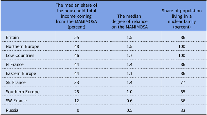
Burnette (2025) reached the same conclusions when analyzing the Les Ouvriers data and showed that the importance of the male head’s income to the households varied across nine regions in Europe.² Depending on the definition, the share of the total household income coming from the male head varied between 25 and 78 percent across the nine regions, with the share being lowest in south-western France and Russia and highest in Britain (Burnette 2025: tbl. 10).³

The purpose of this article is to show two ways to improve how we use wages to compare the MSoL of different populations. I will use the data from Les Ouvriers, as published by Burnette (2024), to illustrate my argument.⁴ Because comparisons of the MSoL are almost always based on the MAMIMOSA, we should focus on this rather than on the total income of the male head of household (which Burnette focused on). Therefore, I revisited the Les Ouvriers books and collected information on the income of the household head coming from their primary occupation(s) (Table 1, first column). The share of the total household income coming from the MAMIMOSA is very closely associated (r = + 0.96, N = 9) with the share coming from the total income of the male head of household, as was presented in Burnette (2025: tbl. 10) (see Table A2 in Supplementary material).

Table 1. Characteristics of the households’ income and structure, by the nine regions

Sources: The first column was calculated from data collected from Le Play (1877) and Société d’économie sociale (1857). The second column combines the data collected from Le Play (1877) and Société d’économie sociale (1857) with the Les Ouvriers data provided by Burnette (2024). The third column was calculated from the Les Ouvriers data provided by Burnette (2024).

Note: The degree of reliance was calculated using the expected share of income, which was calculated using the average number of working-age adults per household.

The data used for the analyses

The data from Les Ouvriers covers only 106 households spread across 16 countries. Further, more than half (60) of the households lived in France. I follow Burnette (2025) in dividing the Les Ouvriers households into groups based on the following nine geographical regions: Britain, the Low Countries, Northern Europe, Northern France, South-Western France, South-Eastern France, Southern Europe, Eastern Europe, and Russia. Even though it is questionable if the households were representative of the underlying populations, the differences in household size in the Les Ouvriers data are comparable to those found in other sources (Burnette 2025: tbl. 1). The reason why Burnette (2025) and I use the Les Ouvriers data is that these household budgets are extremely detailed and include information that is exceedingly rare. For example, the budgets include information on the occupations of all household members, both in the labor market work and in production for their own use. Besides monetary incomes, there are also valuations of payments and production in-kind, as well as valuations of the work put into production for personal use.

The second type of data used in this article is aggregated, country-level data. To ensure comparable country-level data, I have relied on Clio-infra.eu for data on male wages (de Zwart et al. 2015), International Historical Statistics (2013) for the share of population working in the agricultural sector, and the Human Mortality Database (2024) for the demographic indicators. The data coverage of these databases has restricted the sample size for some analyses; seven country-level observations for male wages, and nine countries in five regions for the economic and demographic indicators.⁵

Finally, through extensive literature searches, I have collected 52 estimates of the female/male (F/M) wage ratio in the mid-nineteenth century for 13 European countries (see Table A1 in Supplementary material for further details). I have used the median value for the nine countries with more than one estimate. The sample size when analyzing the effect of including the F/M wage ratio alongside male wages was limited because comparable male wages were currently only available for seven countries.

The sample size is very small, and future work will need to expand on the data to validate my results. Without any additional data, it is not possible to speculate on how the results would change if there were more data available.

The importance of male wages for the material standard of living

Burnette (2025) presents, but fails to comment on, results that have far-reaching implications for the use of male wages in comparisons of the MSoL of households. If one combines the results presented in Tables 1 and 10 in Burnette (2025), it becomes clear that the average share of the total household income coming from the male head of household is strongly, negatively associated (r = –0.86, N = 9) with the average household size (called “family size” in Burnette [2025]) (See Figure A1 in Supplementary material).⁶

The share of the total household income coming from the MAMIMOSA is highest in the populations with the smallest households. Thereby, populations with smaller households are closer to two of the underlying assumptions needed to estimate the MSoL of populations from male wages in general and welfare ratios in particular. First, the notional standard family of four used for welfare ratios is closer to being representative of an average household for populations with smaller households. Secondly, smaller households also meant that the households were more reliant on the income of the male head of household, as is also assumed when using male wages as an indicator of the MSoL of populations.

While it is not self-evident why there would be a negative association between the average household size and the share of the total household income coming from the MAMIMOSA, we should expect a strong negative association between this share and the number of working-age adults in the household. If other working-age adults besides the husband and wife were present, we should expect they contributed to the household income. And, if several adults contributed to the household income, this will, by definition, reduce the share of the total household income coming from the male head of household.

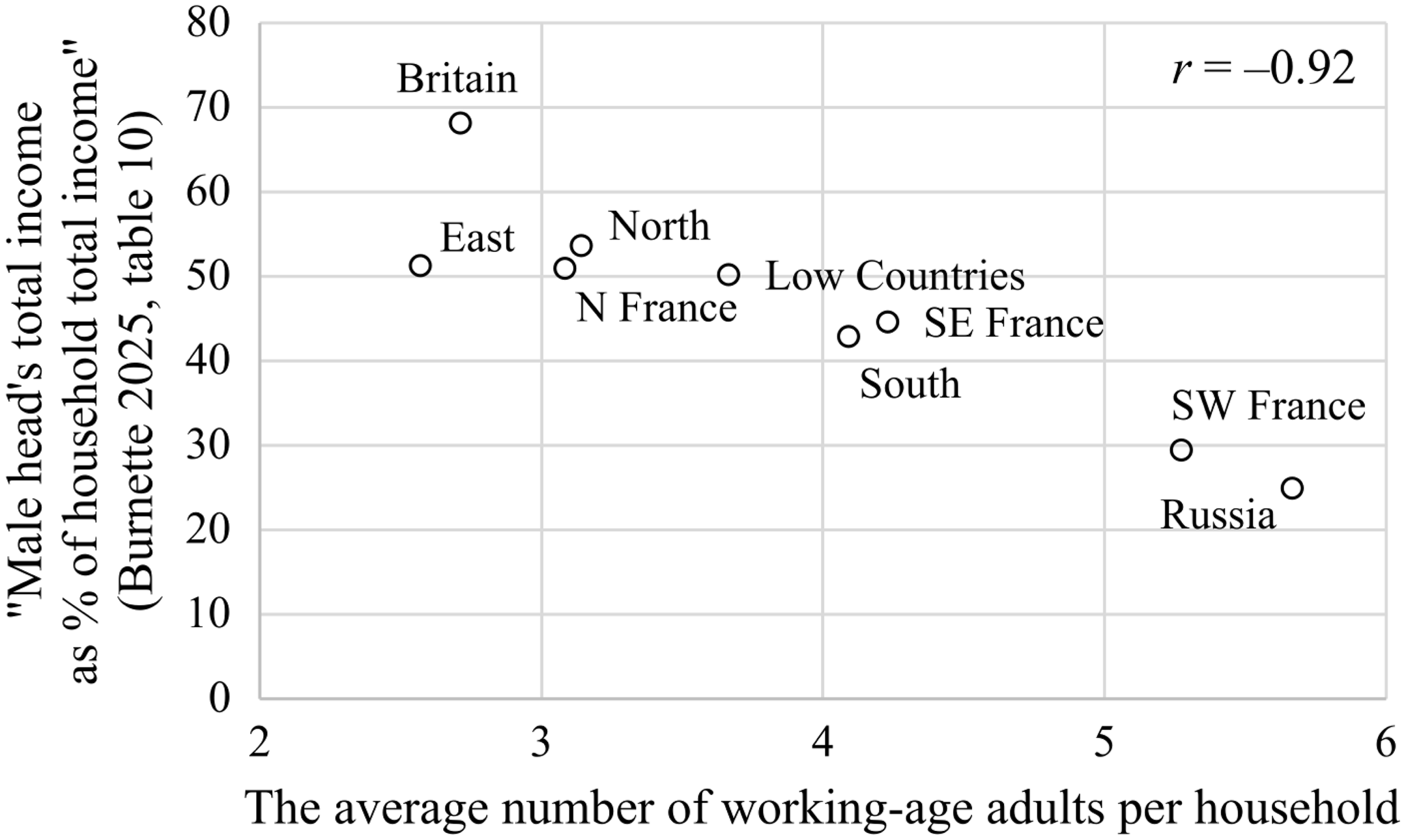
Figure 1 shows the association in the Les Ouvriers data between the average share of the total household income coming from the male head of household and the average number of working-age adults in the household across the nine regions in Burnette (2025). These two indicators have a strong negative association (r = –0.92, N = 9).

Figure 1. The association between the households’ structure and income in nine regions.

Sources: Table 10 in Burnette (2025) and the Les Ouvriers data provided by Burnette (2024).

It is not problematic in and of itself that the average share of the total household income coming from the male head of household is smaller in households including a larger number of working-age adults. In larger households, a greater number of working-age adults contributes to the larger total income needed to sustain the household. However, it is a problem if the degree to which the households are reliant on the income of the male head of household is different in populations with larger households. Specifically, it is a problem for using welfare ratios in comparisons across populations if larger households are less reliant on the MAMIMOSA. A welfare ratio based on the MAMIMOSA will underestimate the MSoL for households that are less reliant on the MAMIMOSA.

Further analysis of the Les Ouvriers data shows that it was, indeed, the case that populations with larger households were also less reliant on the MAMIMOSA. To estimate how reliant the households were on the MAMIMOSA, the observed share of income from this source must be compared to the expected share. As discussed above, the share of the total household income coming from the male head of household will be lower in households with a larger number of working-age adults. If we assume that all working-age adults contribute equally to the household income, it is possible to calculate the share that can be expected to come from the male head. For example, in a household with a husband and wife – two working-age adults – the expected share of the total household income coming from the husband would be 50 percent. In a household with four working-age adults, the expected share would be 25 percent, etc. Figure A2 in the Supplementary material shows the observed share of the total household income coming from the MAMIMOSA plotted against the expected share of the total household income earned by the male head.

The degree to which the households were relying on the MAMIMOSA can be estimated by dividing the observed share by the expected share (Equation 1). The ratio between the two shares includes both the degree to which the male head of household contributed more or less than could be expected and the degree to which the male head of household earned incomes from other sources than his primary occupation.⁷ A ratio above one suggests that the household is to a high degree reliant on the MAMIMOSA.⁸ A ratio equal to one suggests that the MAMIMOSA is equal to the average income from a working-age adult in the household. And, a ratio below one suggests that the household is to a higher degree reliant on the incomes of other members of the household and/or the secondary incomes of the male head of household. Because the indicator captures both the degree of reliance on the MAMIMOSA and the importance of secondary incomes of the male head of household, the substantive interpretation of the ratio is complex, and it is primarily intended as an indicator to be compared across the nine populations.

(1) $$\eqalign{Degree\;of\;& reliance\;on\;the\;IRMCAWTPO \cr & \!\!\!\!\!\!\!\!\!\!\!\!\!\!\! = {{IRMCAWTPO}\over{Total\;household\;income}}-{{1}\over{{The\;number\;of\;working\;age\;adults}}}}\times 100$$

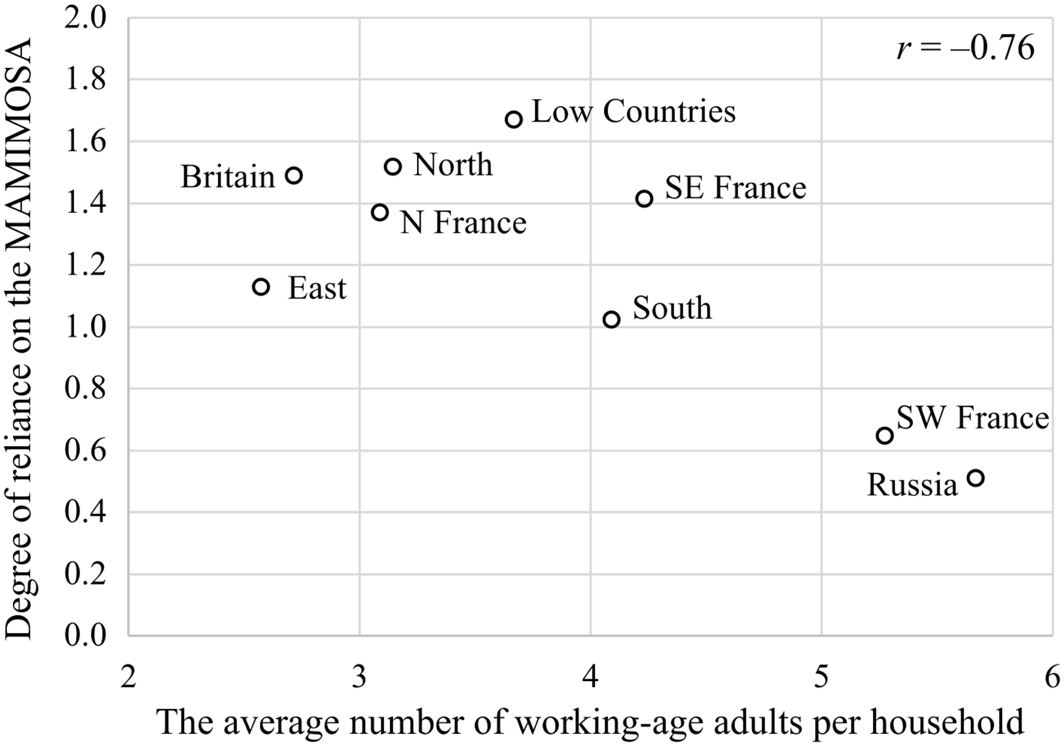
Figure 2 shows the degree of reliance on the MAMIMOSA for the nine regions plotted against the average number of working-age adults per household. The populations in the north and north-western parts of Europe were more reliant on the MAMIMOSA than the populations in the southern and eastern parts. As can also be seen in Figure 2, the degree of reliance on the MAMIMOSA is closely and negatively associated with the average number of working-age adults per household (r = –0.76). However, the degree of reliance on the MAMIMOSA is not as closely related to the average number of working-age adults per household as the average share of the total household income coming from the male head of household. The reason for the weaker association for the reliance on the MAMIMOSA is that this indicator excludes the variation in the importance of the secondary incomes for the male head of household. In general, the secondary incomes of the male head of household were more important in the regions in which the share of the total household income coming from the MAMIMOSA or the total income of the male head was lower (and reversed) (Table A2 in Supplementary material). Britain is an exception to this pattern, combining a high degree of reliance on the MAMIMOSA with secondary incomes of the male head also being important.

Figure 2. The degree of reliance on the MAMIMOSA across the nine regions plotted against the average number of working-age adults per household

Sources: The Les Ouvriers data provided by Burnette (2024) with added data collected from Le Play (1877) and Société d’économie sociale (1857).

Note: The degree of reliance was calculated using the expected share of income, which was calculated using the average number of working-age adults per household.

Guesstimating the degree of reliance on the MAMIMOSA

Because the degree of reliance is so closely associated with the average number of working-age adults in the households, we can use the latter to get an educated guesstimate of how reliant the households in the population were on the MAMIMOSA without having detailed budgets. The average number of working-age adults is, in turn, closely associated with the level of complexity of households in a population (i.e., how common it is to have households with three or more generations, or more than one nuclear family living together). This is illustrated in Table 1, which shows the degree of reliance on the MAMIMOSA for the nine regions along with the share of the population living in a nuclear family. Populations with a high share of nuclear families were more reliant on the MAMIMOSA than populations with a low share.

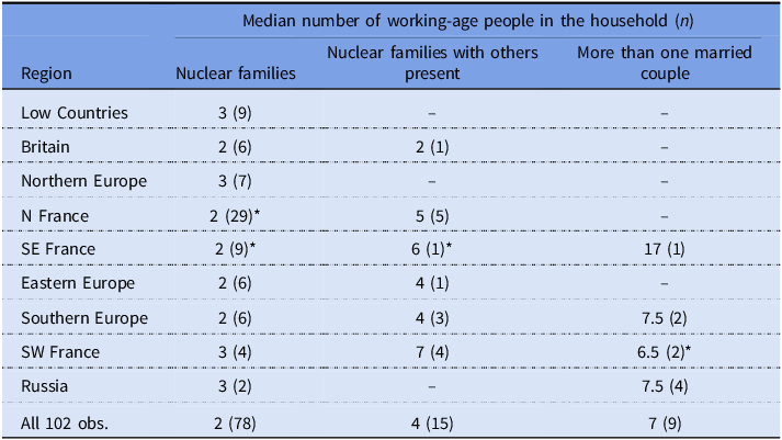
The close association between the complexity of the household and the number of working-age adults present is shown in detail in Table 2. Table 2 shows the median number of working-age people in the households in the Les Ouvriers data separated by region and type of household.⁹ The median number of working-age people is larger in the more complex households across all regions except Britain. (This was a nuclear family living with an elderly person.)

Table 2. Household size and complexity, by the nine regions

Source: Calculated from the Les Ouvriers data provided by Burnette (2024).

Note: I have excluded four households in which the head of household was 65 years old or older because he would not have been counted as a working-age adult. The cells these households would have appeared in are marked with an asterisk.

It is also clear from Table 2 that the complexity of the households increases in the regions further down the list. However, in Table 2, the regions are actually sorted based on the median share of the total household income coming from the MAMIMOSA (see Table 1). This pattern supports the suggestion here that the complexity of households in a population can be used to get an informed guesstimate of how reliant households were on the primary income of the male household head. Therefore, I propose that we can use the complexity of households in a population as a predictor of how reliant the households in this population were on the MAMIMOSA.

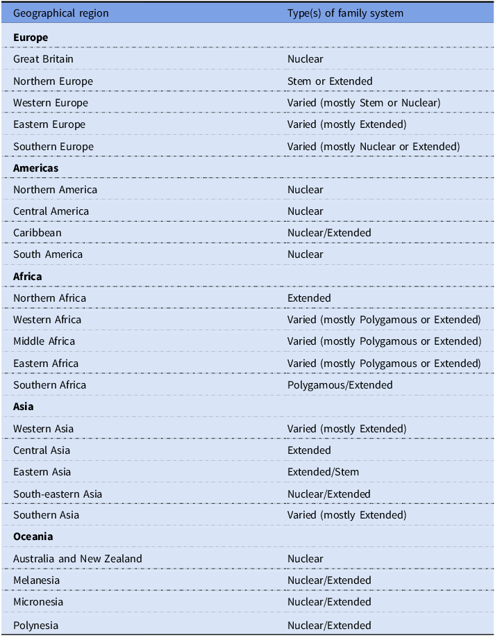
There are clear differences in the complexity of households globally that would make a difference for comparisons based on the MAMIMOSA (Esteve et al. 2024). Rijpma and Carmichael (2016) created a global classification of family systems by combining two compilations of anthropological and ethnographic data (see also Carmichael and Rijpma 2017). Most of the original underlying data were collected during the first half of the twentieth century. However, Rijpma and Carmichael’s (2016) analyses of the data suggested that even though characteristics of family systems might change, there is also persistence over time. The systematic differences between continents and regions seen in Table 3 are sufficiently clear to make it likely that at least some of these differences were present also historically.¹⁰ Therefore, there are reasons to check the historical family systems of any populations included in comparisons of their MSoL based on male wages.¹¹

Table 3. Family systems globally, by geographical region

Sources: Auke Rijpma kindly shared the data used in Rijpma and Carmichael (2016).

However, because the complexity of households in historical populations is often not known, we need a way to estimate this complexity from other indicators. Ruggles (2009: 259) used data from 84 censuses of populations in 35 countries between 1865 and 2007 to show that “a few simple economic and demographic indicators effectively predict most variation in coresidence” with elderly relatives, with coresidence with elderly relatives being used as a measure of the complexity of households in a population.¹² Specifically, the share of the population employed in agriculture and the percentage of the population aged 65 years or older were useful for predicting the coresidence pattern.¹³

The results in Ruggles (2009) suggest that we can use the share of the population employed in agriculture and the percentage of the population aged 65 years or older to estimate the complexity of households in different populations and, therefore, the degree to which households in these populations were reliant on the MAMIMOSA. The share of the population employed in agriculture is a measure of economic diversity and industrialization. The share of the population that is 65 years or older is, in turn, determined by which stage of the demographic transition¹⁴ the population is in.

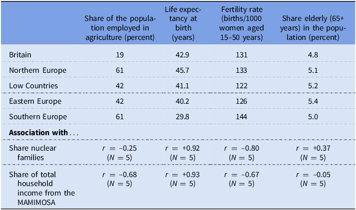
Table 4 shows the share of the population employed in agriculture, the period life expectancy at birth, the fertility rate,¹⁵ and the share of the elderly in the population for the five regions in Burnette (2025) for which data were available. The associations in Table 4 suggest that the period life expectancy at birth and the fertility rate could be useful indicators for guesstimates of how reliant households in a population were on the MAMIMOSA. The share of the population employed in agriculture could also be a useful predictor, seemingly at least partly through another channel than the complexity of the households.

Table 4. Associations between economic and demographic characteristics by five regions

Sources: Share employed in agriculture: International Historical Statistics (2013); the period life expectancy, the fertility rate, and the share of elderly in the population: Human Mortality Database (2024). Share of nuclear families and the share of income from the MAMIMOSA: The Les Ouvriers data provided by Burnette (2024) with added data collected from Le Play (1877) and Société d’économie sociale (1857). See the online Appendix Spreadsheet, “Agricultural population” and “Demography,” for further details (available at OpenICPSR 223 202, https://doi.org/10.3886/E223202V2).

Note: The five regions are represented by the following countries: Britain: Great Britain; Low Countries: Belgium, the Netherlands; North: Denmark, Finland, Norway, Sweden; East: Switzerland; South: Italy.

Because of data availability, the analyses in Table 4 are based on only five observations. Therefore, the results should be considered tentative. However, none of the results in Table 4 contradict the results in Ruggles (2009). Taken together, the results presented here suggest that populations with similar household structures and at similar stages of industrialization and demographic transition are the most comparable if we want to use male wages to estimate their MSoL. Limiting comparisons of the MSoL based on male wages to countries that are similar is clearly restrictive. It is not my opinion that we should limit our comparisons to such cases. However, I do suggest that we can use these results to evaluate when male wages are underestimating the MSoL of a population. The results indicate that the MAMIMOSA underestimates the MSoL of populations with higher fertility rates, lower life expectancy, and a more agricultural economy. These results can be taken into account if we want to compare such populations with those that have lower fertility rates, higher life expectancy, and a more diversified economy.

Access to property also affects the degree of reliance on the MAMIMOSA

Yet another factor that can influence the share of the total household income coming from the MAMIMOSA is the households’ access to property. Obviously, access to property will contribute positively to the MSoL in a direct way. However, access to property will also affect how well the MAMIMOSA works as an indicator of the households’ MSoL in, at least, two ways.

First, households will be less reliant on the MAMIMOSA when there are productive alternative uses of their time, and access to different types of property is necessary for many types of household production (as noted by both Le Play 1879: 249–53, 261, and Burnette 2025: 107; see also Whittle 2024). For example, small-scale farming and animal husbandry were common ways to complement the MAMIMOSA but both require access to property (cf. extensive margin). Secondly, access to different forms of property can increase the productivity of household production (cf. intensive margin). We should, therefore, expect the MAMIMOSA to be a less useful measure of the MSoL for households (and populations) with access to more property. If we want to compare the MSoL of different populations based on the MAMIMOSA, we should check that the populations have access to similar amounts of property (as well as public goods and services).

The F/M wage ratio as an indicator of the material standard of living

Further, I argue that a simplistic formalized model of a household’s sources of MSoL points to a hitherto underutilized indicator: the F/M wage ratio. An advantage of using this indicator alongside male wages is that the F/M wage ratio can be expected to be more important in populations for which male wages are a less useful indicator of the MSoL.

I have based the model on the very comprehensive budgets included in Les Ouvriers. While the simplification exercise only includes labor-based sources of income, I will return to the other sources of income in the conclusions. I will also only include a husband and a wife in the formalization. (In the equations, the terms are separated through subscript m and f.) Again, I will return to how we can reintroduce other household members.¹⁶ As is always the case, the model is a simplification that requires several more or less questionable assumptions. However, I argue that even questionable assumptions are useful if they enable structured conclusions and clarify relevant questions for further research.

In the model, I separate the income from labor into two categories: (a) income from labor market work and from work producing for the market through, for example, farming or knitting, and (b) income from work for production for the household's own use. The first category is what is more often known in historical sources. An algebraic summary of the labor-based sources of income for the households then looks like this:

(2) $$MSo{L_{hh}} = M{I_m} + F{U_m} + H{W_m} + M{I_f} + F{U_f} + H{W_f}$$

$MSo{L_{hh}}$ : the sum of all incomes of the household, hh, as a measure of its MSoL

$MI$ : the market incomes from labor market work or production,

$FU$ : the monetary value of the production for own use,

$HW$ : the monetary value of the housework.

Incomes from labor market work or production for a market, production for own use, and housework can all be separated into the time spent on the task, t, and the “wage” (i.e., the amount of income created from one unit of time spent working on the task), w. The times, t, and the “wages,” w, are differentiated through superscript MI, FU, and HW.

$$MI = {t^{MI}}{w^{MI}}$$

$$FU = {t^{FU}}{w^{FU}}$$

(3) $$HW = {t^{HW}}{w^{HW}}$$

The total available time, T, is fully used doing the different tasks or as unproductive leisure, superscripted L.

(4) $$T = {t^{MI}} + {t^{FU}} + {t^{HW}} + {t^L}$$

I don’t assign any value to leisure because we are studying the MSoL as it can be measured through income (and not the households’ overall utility). The amount of time spent on productive tasks is, therefore, $T - {t^L}$ .

Separating the work-related terms of Equation (1) into the time spent on a task and its “wage” makes the expression look like this:

(5) $$MSo{L_{hh}} = t_m^{MI}w_m^{MI} + t_m^{FU}w_m^{FU} + t_m^{HW}w_m^{HW} + t_f^{MI}w_f^{MI} + t_f^{FU}w_f^{FU} + t_f^{HW}w_f^{HW}$$

While Equation (5) is not obviously more helpful than Equation (1), we can make assumptions allowing us to simplify the expression in Equation (5). In her analyses of the Les Ouvriers data, Burnette (2025: 93) makes one such simplifying assumption and values housework the same as labor market work, meaning ${w^{HW}} = {w^{MI}}$ . This assumption relies on the idea that it is meaningful to value the time spent on other tasks using the foregone income from labor market work that could have been carried out during this time (i.e., other tasks are valued with the opportunity cost using the labor market wage) (Becker 1965).

Further, we can use the same line of argument to value the work spent on production for one's own use, using the foregone income from labor market work (i.e., the opportunity cost). Le Play (1879: 278–79) assigns the value of similar labor market work to the work spent on production for use. The Les Ouvriers data can be used to calculate the ratio between the wage(s) earned in the primary occupation and the (imputed) wage(s) earned from secondary occupations or production for own use. For men, the median ratio is 1.07 (average 1.20, N = 106), and for women, the median ratio is 1.00 (average 1.17, N = 58). Therefore, at least for the households in the Les Ouvriers data, it is reasonable to value time spent on other types of work using the foregone wage for labor market work (i.e., ${w^{FU}} = {w^{MI}}$ ). Using these two opportunity cost assumptions, Equation (5) can be rewritten as:

(6) $$MSo{L_{hh}} = \left( {t_m^{MI} + t_m^{FU} + t_m^{HW}} \right)w_m^{MI} + \big ( {t_f^{MI} + t_f^{FU} + t_f^{HW}} \big )w_f^{MI}$$

The consequence of these two opportunity cost assumptions is, therefore, that it does not matter for the MSoL of the household who is doing how much labor market work, production for own use, or housework. What does matter is the amount of time spent on productive work and the wage of the labor market work.

Next, I will introduce the assumption that the value of work of women compared to the value of work of men can be reasonably described as a constant wage ratio, WR. Assuming a constant wage ratio allows me to substitute the market wage paid to men multiplied by the wage ratio for the market wage paid to women: $w_f^{MI} = w_f^{MI}WR$ . The wage ratio is without a unit and does not need to be adjusted in any way to be comparable across populations. The main advantage of assuming a constant wage ratio is that it allows for using independent empirical estimates of the wage ratio (as I do below).

We can also substitute total time minus time spent on unproductive leisure, $T - {t^L}$ , for the amounts of time spent on labour market work or production, production for own use, and housework (i.e., $T - {t^L} = {t^{MI}} + {t^{FU}} + {t^{HW}}$ ). The final simplified version of Equation (1) then looks like this:

(7) $$MSo{L_{hh}} = \left( {T - t_m^L} \right)w_m^{MI} + \big ( {T - t_f^L} \big )w_m^{MI}WR$$

The MSoL of the household is (in this highly reductive model) determined by three factors:

1. 1. the amount of time spent on productive work, $T - {t^L}$ ,

2. 2. the market wage for men, $w_m^{MI}$ , and

3. 3. the ratio of wages paid to women compared to men, $WR$ .

These three factors are studied individually in three important scholarly works. de Vries (1994) is the seminal work on the consequences for the MSoL from the total amount of time spent on productive tasks (de Vries 1994). Allen’s (2001) article introducing the welfare ratio is a similarly influential work for the study of the consequences for the MSoL from the wage for men for labor market work (or market production) (see also Allen 2015; Allen et al. 2011). Finally, Burnette has written an important work for the study of the ratio of women’s wages compared to men’s (Burnette 2008; for a recent overview of the literature, see de Pleijt and van Zanden 2021). Notably, the simplistic model reminds us that all three perspectives need to be considered jointly if we want to estimate the MSoL.

While the amount of time spent on labor market work and the market wage for men have been thoroughly studied as determinants of the MSoL, not much work has, hitherto, been done on the gender wage ratio as a determinant of the MSoL. Below, I will make a tentative attempt to evaluate if this ratio could be a fruitful avenue for further research.

Evaluating the usefulness of the F/M wage ratio as a measure of MSoL

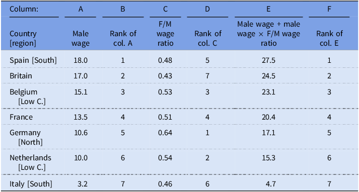
I have gathered estimates of the ratio of the wage paid to women compared to that paid to men in 13 European countries in the mid-nineteenth century (Table A1 in the Supplementary material). For seven of these countries, there were also comparable estimates of the male wage available. Column A in Table 5 shows the wage of male building laborers in the mid-nineteenth century expressed as subsistence ratios (de Zwart et al. 2015). Column B shows the rank number of the countries sorted from highest to lowest male wage. Columns C and D show the ratio between female and male wages and the countries ranked from the highest to the lowest ratio. There is no clear association between the level of the male wage and the size of the F/M wage ratio. In column E, I have combined the male wage and the wage ratio to calculate the total income of one adult man and one adult woman as suggested in Equation (7); $w_m^{MI} + w_m^{MI}WR$ . Column F shows the rank numbers of the countries sorted by the size of this sum from largest to smallest. The ranking is identical when based on the male wage as it is when based on the combination of male and female wages.

Table 5. Using male and female wages as indicators for the standard of living in 7 European countries in the mid-nineteenth century

Sources: Male wage: building laborers’ real wage, median for the years 1850–1859, Clio-Infra.eu (de Zwart et al. 2015); female/male (F/M) wage ratio in the mid-nineteenth century; see Table A1 in the Supplementary material.

This result suggests that the F/M wage ratio does not add anything to our knowledge on the relative ranking of the MSoL of historical populations. The theoretical model, as well as results from present-day populations (e.g., King et al. 2020; Veas et al. 2021), suggest that the wage ratio should add information to comparisons based on only male wages. Also, there are at least two weaknesses in the calculations in Table 5 that should be kept in mind before concluding that the F/M wage ratio does not add any information. First, the calculations are based on seven countries from northern, western, and southern Europe and can, therefore, not necessarily be generalized to other regions. Second, the calculations are based on the assumption that the F/M wage ratio is constant across all sectors of the economy. As can be seen in Table A1 in the Supplementary material, there are reasons to question these assumptions.

Conclusions

In this article, I argue that it is worthwhile to evaluate how reasonable it is to compare the MSoL of different populations based on male wages. Burnette (2025) showed that we should expect that the share of the total household income coming from the male head varied between populations. Here, I have tried to demonstrate that we can get informed guesstimates regarding how reliant households were on the MAMIMOSA by using demographic and economic indicators. Populations with similar household structures, access to similar amounts of private, public, and social capital, and that are at similar stages of industrialization, and the demographic transition will be the most comparable. However, because we know that if we use male wages, we will underestimate the MSoL of populations with higher fertility rates, lower life expectancy, and a more agricultural economy, we can take this into account when making our comparisons.

The results at both the household and the country levels are based on small numbers of observations from a limited geographical area. Obviously, I cannot predict how the results would change if there were more data available. However, even in their current form, the results are valid as a reminder that all comparisons of the MSoL of different populations based on wages should consider all the necessary underlying assumptions.

I also argue in this article that investigating the F/M wage ratio can be an additional way to improve wage-based comparisons of the MSoL of different populations. The tentative results, presented above, could not support a claim that the wage ratio adds information to rankings of the MSoL based on only male wages. However, I still argue that it could be relevant for future research to also consider the F/M wage ratio when comparing the MSoL across populations.

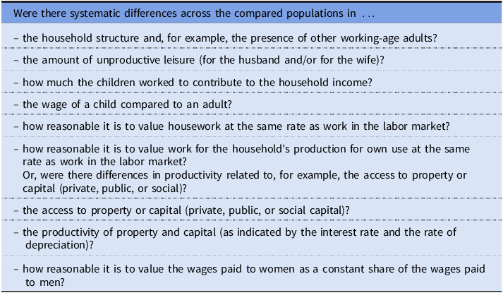
The simplistic model I used to point out the F/M wage ratio as an indicator for the MSoL of households relied on several, more or less plausible assumptions. However, I argue that even the less plausible ones can be useful to us as they highlight important questions for further research. Ideally, all these issues should be taken into account simultaneously. However, even the ones that cannot be investigated in detail for a specific study do provide a possibility for us to be aware of cases where we are likely to overestimate or underestimate the MSoL. Bringing other household members as well as other sources of income back into the picture, the assumptions underlying the simplistic model lead us to the following list of relevant empirical questions (Table 6).

Table 6. List of relevant empirical questions for future studies using male wages to compare the material standard of living across different populations

I do not argue that this list includes all relevant questions for future comparative research into the MSoL of populations. However, I do think it highlights some links to other fields that have not been sufficiently recognized, such as the close association between research into historical household structures and research using male wages as an indicator for the MSoL. The close association between the household structure and the households’ reliance on the income of the male head of household should also remind us that using male wages as an indicator for the MSoL is directly related to research on the nuclear hardship hypothesis (Laslett 1988; van Zanden et al. 2019b).

The simplistic model presented above suggests that the most relevant factor for the MSoL, besides the male and female wages, is the time spent on productive work. In the model, I assume that the labor market wage can be used as an estimate of the productivity of all types of work. Therefore, it is important to note that the time spent on productive work should include all tasks (i.e., labor market work, production for the market and for own use, housework, etc.). What is interesting for comparisons of the MSoL is whether or not there were systematic differences in the total amount of work or, inversely, if there were systematic differences in the time spent on unproductive leisure. There is, of course, research attempting to estimate this (e.g., de Vries 1994; Allen and Weisdorf 2011; Muldrew 2011; Gary and Olsson 2020). However, to the best of my knowledge, there is not yet a consensus on how this should be estimated or any large-scale comparative studies.

I am not claiming to be the first to point out the importance of including women in research into the MSoL of populations. For example, Szołtysek and Poniat (2024) argue that the level of gender (and age) equality in a country historically can be used to predict both gender equality today and the country’s long-term economic development. van Zanden et al.’s (2019a) book Capital Women similarly argues for the importance of women’s economic empowerment and agency in the long-term economic development in Europe. The positive effects they are arguing for have, indeed, been confirmed in research on present-day low-income countries (Balasubramanian et al. 2024).

This earlier research has focused on the positive long-term effects of gender equality on the MSoL. What I want to add to the literature comparing the MSoL of historical populations is the suggestion that the F/M wage ratio could be a useful indicator also for the short term and, especially, in cross-sectional comparisons.

I have shown that the assumptions needed to use male wages as an indicator of the MSoL of historical populations are stricter than have previously been acknowledged. However, I have also shown possible ways to move forward while improving the reliability of this indicator by evaluating the necessary assumptions.