

1. Introduction
The recent pandemic hit many economies in environments of low interest rates and high debt ratios. Central banks worldwide have adopted extraordinary measures, restoring the role of fiscal macroeconomic stabilisation to jumpstart recovery. The subsequent inflation surge – sourced by the combination of multiple shocks – restored not only standard monetary operations, but also debates about the role of fiscal policy and the way back to fiscal normalisaton. In the Euro Area (EA), these debates are even more fierce as the European Monetary Union (EMU) has established a special case of institutional framework – formalised by the 1992 Maastricht Treaty – that is complex to track and yet to be completed (see Reichlin et al. Reference Reichlin, Ricco and Tarbé2023; Pappa, Reference Pappa2020). Unlike national frameworks, the EMU features the coexistence of a single common, credible, and independent central bank targeting aggregate inflation, while fiscal policy remains fragmented at the member level under common rules. This unique design shapes a new form of policy interactions with the European Central Bank (ECB) acting on its price mandate, while national fiscal authorities treat inflation as given. In this multi-level setting, agents’ beliefs and uncertainty about policy credibility and coordination strategies gains major relevance to determine stability and sustainability outcomes (see Sims, Reference Sims1994; Cochrane, Reference Cochrane1998).Footnote 1 A comprehensive account of policy regimes for European countries is still missing.Footnote 2
We contribute to this debate using a model-based general equilibrium approach, where the history of monetary-fiscal interactions is driven by Markov-switching (MS) policy mix regimes (Bianchi and Ilut, Reference Bianchi and Ilut2017). These recurrent regimes shape macroeconomic outcomes, influencing growth, debt, and inflation. Agents form expectations based on the probabilistic distribution of future regime changes (Bianchi, Reference Bianchi2013), which enter their decisions and in turn affect equilibrium allocations. Therefore, agents’ beliefs and uncertainty about the duration and stability of policy regimes are a key aspect to be considered, possibly shaping regime transitions and macroeconomic dynamics.
We estimate a Dynamic Stochastic General Equilibrium (DSGE) for Italy and France from the 1950s to 2019. We select these countries as case studies of high fiscal imbalances and distinct yet comparable macroeconomic policy facts. Both experienced major shifts in monetary and fiscal policies, including periods of fiscal expansions, monetary tightening, and European integration. This allows for a comparative analysis of policy regimes and their responses to macroeconomic shocks. Moreover, as Italy has faced greater debt management challenges whereas France has relied on more fiscal space, the comparison enables an analysis of how fiscal constraints impact policy effectiveness.
The model allows the identification of alternative combinations of policy coordination or conflict regimes, which we interpret in terms of active/passive monetary and fiscal policy (Leeper, Reference Leeper1991), where an active behaviour identifies a leading authority, which sets interest rates (active monetary) or primary deficits (active fiscal) to control inflation or stabilise macroeconomic fluctuations (respectively), independently of inflation and debt dynamics. In cases of policy coordination, an active policy behaviour by one authority forces the other one to adopt a passive behaviour and accommodate: when monetary policy is active, the fiscal authority has to ensure primary surpluses adjust to stabilise debt; when fiscal policy is active, the central bank has to accommodate fiscal imbalances, allowing inflation to adjust and ensure debt sustainability. Hence, an Active Monetary-Passive Fiscal Policy mix (AM/PF) is a regime where the central bank controls inflation and the fiscal authority passively accommodates by adjusting primary surpluses to debt. In this regime, fiscal imbalances are backed by fiscal adjustments. A passive monetary-active fiscal policy mix (PM/AF) is then a regime where the fiscal authority is not constrained by its budget balance and the monetary authority allows inflation to stabilise debt. In these two policy interaction frameworks, inflation and debt are uniquely determined. However, we also allow the model to potentially generate cases of policy conflict scenarios (active monetary-active fiscal, passive monetary-passive fiscal), whose solutions - in absence of policy switches - would not exist or be indeterminate, respectively. Notably, we restrict the fiscal and monetary switches to occur at the same dates, hence they are not independent over time.
The model, specified as a closed economy, also incorporates deterministic monetary shifts to the EMU in 1999 and the Effective Lower Bound (ELB) regime in 2009. Post-EMU, the monetary instrument is defined at the EA level, thus responding to area-wide targets. The ELB is modelled as a monetary state with nominal interest rates set at zero, constraining the central bank’s response to inflation.Footnote 3 This framework unifies pre-EMU dynamics and the common currency period, which is crucial for identifying policy regimes over long horizons. However, the closed economy assumption to model European economies abstracts from cross-country dynamics, linked by exchange rates (pre-EMU) and a common central bank (post-EMU).
By estimating the model, we draw a narrative of policy interaction strategies for France and Italy in the post-World War II era. In both countries, an initial PM/AF regime describes sustained growth, the run-up of inflation, primary deficits, and low fiscal imbalances. The transition to an AM/PF regime coincides with the convergence to the monetary union, reinforcing the separation between a central bank committed to inflation control and fiscal authorities bound by European rules. France shifted earlier, by pegging the Franc to the Deutsche Mark under the European Exchange Rate Mechanism (ERM) in 1979. This significant turn not only helped restore exchange rate stability but it also imported the Bundesbank’s anti-inflationary credibility to signal a stronger commitment to low inflation. Mitterrand’s shift toward fiscal consolidation in 1987 accommodated the transition, with the aim to sustain the new active monetary strategy and meet the fiscal convergence criteria of the Maastricht Treaty. Italy, by contrast, experienced a more gradual and fragile adjustment: although it entered the ERM alongside France in 1979, it faced repeated currency tensions and exited the mechanism in 1992, only rejoining in 1996. This shift was further complicated by the delayed “divorce” between the Bank of Italy and the Treasury, ending the automatic monetisation of public debt only in the 1990s as part of a broader reform to strengthen central bank independence and qualify for EA membership.
The ELB later constrained the ECB action, prompting France to adopt active fiscal measures to counter deflation, whereas Italy delayed its transition to the end of the sovereign debt crisis, due to austerity under Monti’s government.
Model-based regime-conditional simulations—to fiscal, monetary, demand, and supply shocks—reveal that the PM/AF regime in France led to price volatility but stabilised debt, whereas the AM/PF regime achieved disinflation at the cost of rising debt. In Italy, by contrast, procyclical fiscal policy in downturns exacerbated imbalances, aggregate volatility, and low growth, especially under the PM/AF regime. These differences are closely linked to the role of fiscal space in our regime-switching framework. Tighter fiscal constraints in Italy—stemming from persistently high debt ratios—induced fiscal authorities to resort more often to procyclical consolidations in downturns, which amplified output volatility and debt accumulation. By contrast, France’s comparatively larger fiscal space allowed it to accommodate shocks, leading to smoother debt dynamics and a more supportive role for fiscal policy within the same monetary environment.
We then simulate belief scenarios (Bianchi and Ilut, Reference Bianchi and Ilut2017; Bianchi and Melosi, Reference Bianchi and Melosi2014) to isolate the role of agents’ expectations about future policy shifts in shaping model dynamics. We first run scenarios on agents’ confidence about transitioning from a PM/AF to a AM/PF regime. We show that when agents anticipate the transition, they behave already as if they were under AM/PF conditions. Hence, the credibility of announcing a different policy can significantly affect already the efficacy of the current policy stance. Then, we simulate scenarios where agents face uncertainty about the duration of the AM/PF regime - while still observing the regime in place in each period. Modelling this as a process where agents cannot immediately discern whether AM/PF is temporary or persistent, we find a gradual adjustment to the change in regime after the shift dates.
The remainder of this paper is organised as follows. Section 2 reviews the literature, and Section 3 recovers relevant stylised facts for monetary and fiscal policy historical regularities in the French and Italian data. The model is presented in Section 4. Section 5 provides the estimation results, extracts policy regimes, interprets regime-specific impulse responses, and builds scenarios on policy credibility and agents’ uncertainty. Section 6 discusses policy recommendations and Section 7 concludes.
2. Literature review
This study relates to three strands of the literature. First, the Fiscal Theory of the Price Level (FTPL) explains fiscal inflation (Sims, Reference Sims2011). Following the seminal contribution of Sargent and Wallace (Reference Sargent and Wallace1981), various studies (Sims, Reference Sims1994; Woodford, Reference Woodford1994, Reference Woodford1995, Reference Woodford2001) placed fiscal policy in coordination with the monetary authority. Leeper (Reference Leeper1991) defines the conditions for the uniqueness and existence of model solutions under combinations of policy regimes.Footnote 4 The latter have been studied both in isolation (Cochrane, Reference Cochrane1998, Reference Cochrane2001; Bhattarai et al. Reference Bhattarai, Lee and Park2012) and within a unified general equilibrium framework of power imbalances between two policy authorities (Fragetta and Kirsanova, Reference Fragetta and Kirsanova2010; Davig and Leeper, Reference Davig and Leeper2011; Bianchi and Melosi, Reference Bianchi and Melosi2017).
While the empirical validation of the FTPL is well established for the US, it is not fully explored for European countries. Reichlin et al. (Reference Reichlin, Ricco and Tarbé2023) explains how the European special institutional setting in Europe determines aggregate/domestic fiscal and monetary outcomes. Kliem et al. (Reference Kliem, Kriwoluzky and Suarez2016) elect the central bank independence process as a turning point between monetary-fiscal policy regimes. Jarociński and Maćkowiak (Reference Jarociński and Maćkowiak2018) and Bianchi et al. (Reference Bianchi, Melosi and Rogantini-Picco2022) study policy interaction in the EMU using a two-country DSGE model.Footnote 5 We inherit the general equilibrium approach within a closed economy framework to cover the long mixed history of Treasury-Central Bank agreements, monetary policy independence, and the growing fiscal instability of the two European economies.
Second, we build upon the empirical literature on the interaction between monetary and fiscal feedback rules. Based on the seminal work by Bohn (Reference Bohn1998), several works have estimated fiscal rules in isolation to test debt sustainability (see Bohn (Reference Bohn2008) and Canzoneri et al. (Reference Canzoneri, Cumby and Diba2011) for the US; Melitz (Reference Melitz2000), Mendoza and Ostry (Reference Mendoza and Ostry2008), Ghosh et al. (Reference Ghosh, Kim, Mendoza, Ostry and Qureshi2013), Mauro et al. (Reference Mauro, Romeu, Binder and Zaman2015), and Aldama and Creel (Reference Aldama and Creel2022) for a panel of advanced and emerging economies; Favero and Monacelli (Reference Favero and Monacelli2005) and Paniagua et al. (Reference Paniagua, Sapena and Tamarit2017) in nonlinear settings; Aldama and Creel (Reference Aldama and Creel2020) for France under MS regimes).Footnote 6 Davig and Leeper (Reference Davig and Leeper2006) introduces the simultaneous consideration of a monetary policy rule, which was applied, among others, by Cevik et al. (Reference Cevik, Dibooglu and Kutan2014) to a sample of emerging European economies. However, such reduced-form estimates are subject to a simultaneity bias arising from failing to bring the forward-looking nature of nominal debt valuation (Leeper and Li, Reference Leeper and Li2017). We use a fully specified DSGE framework to account for the general equilibrium determination of fiscal/monetary policy mix regimes.
Finally, our study borrows from the literature on the role of agents’ beliefs over policy mix regimes. MS-DSGE models provide a good understanding of how agents’ decision rules are affected by the degree of credibility of the changing policy stance (Sims, Reference Sims1982). Agent’s beliefs are relevant both within regimes and as a source of shifts over them (for monetary policy see Schorfheide (Reference Schorfheide2005), Fernández-Villaverde et al. (Reference Fernández-Villaverde, Guerron-Quintana and Rubio-Ramírez2010), Liu and Waggoner (Reference Liu and Waggoner2011) and Foerster (Reference Foerster2015, Reference Foerster2016); for the monetary/fiscal policy mix Davig and Leeper (Reference Davig and Leeper2006, Reference Davig and Leeper2007), Bianchi and Ilut (Reference Bianchi and Ilut2017) and Bianchi and Melosi (Reference Bianchi and Melosi2017)). Moreover, Davig and Leeper (Reference Davig and Leeper2007), Farmer et al. (Reference Farmer, Waggoner and Zha2009), Ascari et al. (Reference Ascari, Florio and Gobbi2020) show that MS models explain expanded regions of equilibrium determinacy through the role of expectations across regimes. We use this framework to simulate scenarios of agents’ beliefs on the future of the policy mix.
3. Narratives on the post-war policy mix
We present fiscal and monetary stylised facts for France and Italy by drawing a narrative over historical policy events characterising the last few decades. Figures 1 and 2 show the evolution of inflation, GDP growth, nominal interest rates, the primary deficit-to-debt ratio as a measure of the fiscal stance (Sims, Reference Sims2011), the debt-to-GDP ratio as an index of fiscal sustainability, and the ex-post real interest rate to measure the debt service cost.Footnote 7
During the 1955–1980 period, France maintained a low debt-to-GDP ratio primarily due to high inflation (inflation tax) and low real rates, despite running primary deficits. Devaluation events in 1958 and 1969 were used to boost growth and offset the lack of competitiveness, although they contributed to economic overheating and inflation. Monetary policy was conducted through quantitative controls on money and credit (Monnet, Reference Monnet2014), due to the rigid separation of the financial system. Following the government of Charles de Gaulle (Les Trente Glorieuses), three policy attempts were made to tackle the 1974–75 recession and the inflation-depreciation cycle. First, a countercyclical fiscal stance led to a significant fiscal balance deterioration in 1975–76. In response to rising inflation and worsening fiscal and external imbalances, the government introduced an austerity package in 1976, known as the Plan Barre, which resulted in higher inflation and deficits. The inflation peaked further with the second oil shock in 1979–1980. Later, in 1981–82, Mitterrand launched the politique de relance, inspired by the Keynesian Programme Commun, implementing expansionary fiscal measures to boost demand and reduce unemployment, but with negative consequences on the external current account, fiscal imbalances, and inflationary pressures were negative. The franc was devaluated in 1981, 1982, and 1983.

Figure 1. Monetary and fiscal policy facts—France. The top panel displays French data for inflation, interest rate and GDP growth. The bottom plot displays the primary deficit-to-debt, the ex-post real interest rates, and the debt-to-GDP ratios. Sample: 1955–2019, annual frequency.
From early 1983, a significant shift in French economic policy occurred (Artus et al. Reference Artus, Avouyi-Dovi, Bleuze and Lecointe1991). A broad adjustment programme was adopted to eliminate the trade deficit within two years and restore fiscal balance. This period, known as tournant de la rigeur or the austerity turn (Martin et al. Reference Martin, Tytell and Yakadina2011), marked profound changes in the French monetary policy system, including a quasi-fixed exchange rate under the ERM aimed at achieving nominal convergence with Germany.Footnote 8 A firm policy to uphold the franc’s external value, known as franc fort or exchange rate targeting, led to disinflation and exchange rate stability by 1987 (Smets, Reference Smets2007). This balanced policy mix was implemented in the context of growing financial integration, culminating in 1987 with the adoption of a monetary policy mechanism based on interest rate variations and liberalised credit markets.
However, the structural improvement of fiscal accounts was hindered by an economic slowdown, lower revenues, and rising interest payments on growing public debt. As the 1997 deadline for the monetary union approached, in 1994, the authorities adopted a five-year budgetary plan (Public Finance Programming Law) to meet the fiscal convergence criteria of the Maastricht Treaty. This law contributed to a decline in the government deficit and public debt stabilisation. In 1999, although adopting the common currency led to a period of low interest rates, the increased fiscal deficit combined with lower inflation led to an upward trend in the debt-to-GDP ratio. In 2003–2007, France was placed under Excessive Deficit Procedures (EDP) to enforce significant fiscal adjustments. In 2008, with the global financial crisis the ECB responded by lowering interest rates to the ELB and implementing asset purchases measures. Despite consolidation announcements under Fillon and Hollande, government deficits remained high.
Moving to Italy, the 1950s initiated a period of sustained economic development (the 1953–68 economic miracle), supported by monetary and fiscal stability. Monetary policy instruments at the time included discount rates, central bank advances, and credit controls. Since 1963, the Bank of Italy’s official interest rates were set by the Treasury, and public debt was entirely monetised. A prudent fiscal stance, favourable macroeconomic environment, and low real rates resulted in low debt-to-GDP ratios. However, the 1960s ended with severe economic difficulties. The collapse of the Bretton Woods System in 1971 led to a switch to a floating exchange regime and several devaluations of the lira. This, combined with a sharp rise in oil prices, caused a period of stagflation.Footnote 9 Inflation peaked at 19.2% in 1980, heavily impacting debt dynamics and fiscal imbalances. In 1979, Italy joined the ERM to stabilise inflation.

Figure 2. Monetary and fiscal policy facts—Italy. The top panel displays Italian data for inflation, interest rate, and GDP growth. The bottom panel displays the primary deficit-to-debt, the ex-post real interest rates, and the debt-to-GDP ratios. Sample: 1950–2019, annual frequency.
The divorce between the Bank of Italy and the Treasury in 1981 marked the beginning of a significant shift in policy to curb inflation (Passacantando, Reference Passacantando1996), in line with the international tendencies (Clarida et al. Reference Clarida, Gali and Gertler1998). This separation freed the central bank from the obligation to buy unsold government securities. In 1983, capital controls were dismissed, and the Bank of Italy moved away from domestic credit targets, using open-market operations as the primary tool for monetary intervention. This marked a transition from government-oriented to market-oriented operations. The introduction of an efficient auction system for treasury bills and a functioning interbank deposit market led to the creation of a true money market.
Despite these changes, the monetary reform was gradual and slow (Fratianni and Spinelli, Reference Fratianni and Spinelli1997). The central bank did not immediately stop buying government securities in the primary market, and the Treasury did not immediately cease setting base rates. By 1989, the minimum purchase prices for government securities were eliminated, and the Bank of Italy adopted an intermediate monetary target to obtain disinflation, reducing inflation to 6%.Footnote 10 The ERM participation enhanced the role of the nominal exchange rate, with the lira entering the narrow band of the ERM and full liberalisation of short-term capital movements. Nominal interest rates became an effective intermediate target for monetary policy. However, an expansionary fiscal stance coupled with rising interest rates led to a debt explosion, with the debt-to-GDP ratio rising from 50 in 1980 to 88% in 1990, causing further inflationary pressures and limited economic recovery. Although Italy achieved price stability, it failed to control public finances (Bartoletto et al. Reference Bartoletto, Chiarini and Marzano2014).
The Bank of Italy gained operational independence in 1992 and began explicitly targeting inflation. In 1993, it started using an interest rate corridor to guide monetary policy. The signing of the Maastricht Treaty in 1992 marked a significant shift in fiscal policy (Paesani and Piga, Reference Paesani and Piga2002; Balassone et al. Reference Balassone, Francese and Pace2013), leading to reforms aimed at adjusting public finances to join the EMU in 1997, such as Reform Amato in 1992 and Reform Dini in 1995. Despite these efforts, the EMS currency crisis and rising risk premiums on Italian bonds caused the debt ratio to peak at 114% in 1994 (Paesani and Piga, Reference Paesani and Piga2002).
Throughout the period leading up to the global financial crisis, Italy’s policy was characterised by inflation targeting, supported by fiscal measures, resulting in low inflation but high real interest rates and peaking debt-to-GDP ratios. In 2009, policy rates hit the ELB while the fiscal authority pursued austerity measures until the end of the sovereign debt crisis in 2012.
4. The model
Our framework builds on a standard monetary DSGE model in the tradition of Lubik and Shorfeide (Reference Lubik and Shorfeide2004) and Clarida et al. (Reference Clarida, Galí and Gertler2010), augmented by MS policy rules capturing recurrent monetary/fiscal policy mix regimes (Bianchi and Ilut, Reference Bianchi and Ilut2017).
We consider a production economy subject to nominal rigidities à la Rotemberg (Reference Rotemberg1982). Sticky prices introduce revaluation effects and channels for policy interactions, implying that monetary policy can influence real interest rates and, in turn, debt dynamics. We also introduce a maturity structure for government debt, external habits in consumption, and inflation indexation. Rules on tax revenues and government expenditure describe fiscal policy. Monetary policy is described by an augmented Taylor rule, accounting for the switch to the monetary union and the ELB on nominal interest rates.
Policymakers’ decisions - the monetary policy rule and tax rule - change between active and passive behaviours according to a two-state MS process,
 $\xi ^p$
, identifying policy mix regimes. They evolve according to the transition matrix
$\xi ^p$
, identifying policy mix regimes. They evolve according to the transition matrix
 $H^p$
, as defined in Table 1, collecting transition probabilities across regimes. Since 2009, the monetary policy is constrained and set at the ELB.
$H^p$
, as defined in Table 1, collecting transition probabilities across regimes. Since 2009, the monetary policy is constrained and set at the ELB.
Table 1. Priors and posteriors of the model parameters

Notes: The table reports the prior specification for model parameters (functional form, mean, standard deviation), and the posterior estimates (modes, means and 90% confidence intervals), for France and Italy. In the prior distribution specification, {G, N, B, IG, Dir} correspond to gamma, normal, beta, inverse gamma, and Dirichlet distribution, respectively.
The model equilibrium conditions are in Appendix A, linearised in Appendix C around the steady state (Appendix B). In Appendix D model variables are mapped to the data, which are described in Appendix E. Appendix F presents the forecast error variance decomposition of key model variables, whereas Appendix G runs model diagnostics.
4.1 Agents and decision problems
The structure of the economy is as follows. A representative household consumes, saves, and supplies labour. The final output is assembled by a competitive final good producer who uses a continuum of intermediate goods manufactured by monopolistic competitors as inputs. Intermediate goods producers rent labour from households and set prices à la Rotemberg (Reference Rotemberg1982). Finally, the central bank fixes the one-period nominal interest rate, while the government sets taxes and determines government expenditures. Ten shocks hit the economy: a preference shock, a technology shock, a cost-push shock, and seven policy shocks.
4.1.1 Households
The representative household’s preferences, logarithmic in consumption
 $C_t$
and linear in labour
$C_t$
and linear in labour
 $h_t$
, are described by the following discounted utility function:
$h_t$
, are described by the following discounted utility function:
 \begin{equation} \mathbb{E}_0\Bigg \{\sum _{t=0}^{\infty } \beta ^t e^{d_t} \Big [\log \big(C_t - \Phi C^A_{t-1}\big) - h_t\Big ] \Bigg \} \end{equation}
where preferences exhibit external habits defined on lagged aggregate consumption
 $\Phi C_{t-1}^A$
, with
$\Phi C_{t-1}^A$
, with
 $\Phi \in [0,1)$
denoting the degree of habit formation. The preference shock
$\Phi \in [0,1)$
denoting the degree of habit formation. The preference shock
 $d_t$
follows an AR(1) process:
$d_t$
follows an AR(1) process:
 $d_t = \rho _d d_{t-1} + \sigma _d \varepsilon _t^d$
.
$d_t = \rho _d d_{t-1} + \sigma _d \varepsilon _t^d$
.
Agents have access to two kinds of government bonds, differing in maturity: a one-period bond in zero net supply
 $B^s_t$
and a long-period bond in non-zero net supply
$B^s_t$
and a long-period bond in non-zero net supply
 $B_t^m$
.Footnote
11
Short- and medium-term bonds’ prices are respectively given by
$B_t^m$
.Footnote
11
Short- and medium-term bonds’ prices are respectively given by
 $P^s_t$
and
$P^s_t$
and
 $P_t^m$
, and
$P_t^m$
, and
 $R_t=\frac {1}{P^s_t}$
and
$R_t=\frac {1}{P^s_t}$
and
 $R^m_{t+1}=\frac {1+\rho P^m_{t+1}}{P^m_t}$
are the respective nominal interest rates. The price recursion for long-term bonds is defined as
$R^m_{t+1}=\frac {1+\rho P^m_{t+1}}{P^m_t}$
are the respective nominal interest rates. The price recursion for long-term bonds is defined as
 $P_{t+j}^{m-j} = \rho ^j P_{t+j}^m$
, where
$P_{t+j}^{m-j} = \rho ^j P_{t+j}^m$
, where
 $\rho \in [0,1]$
controls the degree to which the maturity of bonds decreases and yields the average debt maturity of
$\rho \in [0,1]$
controls the degree to which the maturity of bonds decreases and yields the average debt maturity of
 $(1-\beta \rho )^{-1}$
. With
$(1-\beta \rho )^{-1}$
. With
 $P_t$
as the consumer price, households receive labour income
$P_t$
as the consumer price, households receive labour income
 $P_t W_t h_t$
, pay lump-sum taxes
$P_t W_t h_t$
, pay lump-sum taxes
 $T_t$
, gain profits from firms
$T_t$
, gain profits from firms
 $P_t D_t$
, and lump-sum government transfers
$P_t D_t$
, and lump-sum government transfers
 $TR_t$
. The nominal flow budget constraint for households is:
$TR_t$
. The nominal flow budget constraint for households is:
 \begin{equation} P_t C_t + P_t^{m} B_{t}^m + P^s_t B^s_t = P_t W_t h_t + B^s_{t-1} + \big(1+ \rho P_t^m\big) B^m_{t-1} + P_t D_t -T_t+ TR_t \end{equation}
Then, the bond-pricing equations for short- and long-term securities are:
 \begin{align} 1 = \beta \mathbb{E}_t \bigg \{ e^{d_{t+1} - d_{t}} \frac {u_{c}(t+1)}{u_{c}(t)} \frac {R_{t}}{\Pi _{t+1}} \bigg \} \\[-8pt] \nonumber \end{align}
 \begin{align} 1 = \beta \mathbb{E}_t \bigg \{ e^{d_{t+1} - d_{t}} \frac {u_{c}(t+1)}{u_{c}(t)} \frac {R_{t+1}^m}{\Pi _{t+1}} \bigg \} \\[6pt] \nonumber \end{align}
where
 $u_c(t) = C_{t} - \Phi C^A_{t-1}$
is the marginal utility of consumption and
$u_c(t) = C_{t} - \Phi C^A_{t-1}$
is the marginal utility of consumption and
 $\Pi _{t} = \frac {P_t}{P_{t-1}}$
is the inflation rate. Combining these two conditions, we derive the no-arbitrage condition
$\Pi _{t} = \frac {P_t}{P_{t-1}}$
is the inflation rate. Combining these two conditions, we derive the no-arbitrage condition
 $R_{t} = \mathbb{E}_t \{ R_{t+1}^m\}$
. Finally, the labour supply condition is
$R_{t} = \mathbb{E}_t \{ R_{t+1}^m\}$
. Finally, the labour supply condition is
 $W_t = C_{t} - \Phi C^A_{t-1}$
.
$W_t = C_{t} - \Phi C^A_{t-1}$
.
4.1.2 Firms and price setting
The production sector is populated by a continuum of monopolistically competitive firms and perfectly competitive final goods producers. The first produce intermediate differentiated goods
 $Y_t(j)$
with
$Y_t(j)$
with
 $j \in [0,1]$
, which are combined in a final good
$j \in [0,1]$
, which are combined in a final good
 $Y_t$
through CES technology,
$Y_t$
through CES technology,
 $Y_t = \Big ( \int _{0}^1 Y_t(j)^{1-\nu _t} dj \Big )^{\frac {1}{1-\nu _t}}$
, where
$Y_t = \Big ( \int _{0}^1 Y_t(j)^{1-\nu _t} dj \Big )^{\frac {1}{1-\nu _t}}$
, where
 $\frac {1}{\nu _t}$
is the time-varying elasticity of substitution for intermediate goods. The latter translates into a price markup shock
$\frac {1}{\nu _t}$
is the time-varying elasticity of substitution for intermediate goods. The latter translates into a price markup shock
 $\mu _t = \frac {\kappa }{1+\iota \beta } \log \big (\frac {1-\nu }{-\nu _t}\big )$
, where
$\mu _t = \frac {\kappa }{1+\iota \beta } \log \big (\frac {1-\nu }{-\nu _t}\big )$
, where
 $\kappa = \frac {1-\nu }{\nu \psi \Pi ^2}$
,
$\kappa = \frac {1-\nu }{\nu \psi \Pi ^2}$
,
 $\iota$
controls the indexation to lagged inflation,
$\iota$
controls the indexation to lagged inflation,
 $\psi$
determines the degree of nominal price rigidity,
$\psi$
determines the degree of nominal price rigidity,
 $\nu$
and
$\nu$
and
 $\Pi$
represent the steady-state levels of
$\Pi$
represent the steady-state levels of
 $\nu _t$
and
$\nu _t$
and
 $\Pi _t$
, respectively. Finally, we assume an exogenous process for the markup shock
$\Pi _t$
, respectively. Finally, we assume an exogenous process for the markup shock
 $\mu _t = \rho _\mu \mu _{t-1} + \sigma _\mu \varepsilon _t^\mu$
.
$\mu _t = \rho _\mu \mu _{t-1} + \sigma _\mu \varepsilon _t^\mu$
.
Intermediate firms are price takers in factor markets and price makers in the goods market. Given technology, profit maximisation yields the demand for intermediate inputs,
 $Y_t(j) = \Big ( \frac {P_t(j)}{P_t} \Big )^{\frac {1}{\nu _t}} Y_t$
, where
$Y_t(j) = \Big ( \frac {P_t(j)}{P_t} \Big )^{\frac {1}{\nu _t}} Y_t$
, where
 $P_t(j)$
is the price of intermediate good
$P_t(j)$
is the price of intermediate good
 $j$
and
$j$
and
 $P_t$
the price of final goods. Intermediate producers operate under monopolistic competition and are endowed with the production technology
$P_t$
the price of final goods. Intermediate producers operate under monopolistic competition and are endowed with the production technology
 $Y_t(j) = A_t h_t(j)^{1-\alpha }$
, where labour is the only input,
$Y_t(j) = A_t h_t(j)^{1-\alpha }$
, where labour is the only input,
 $\alpha \in (0,1)$
and
$\alpha \in (0,1)$
and
 $A_t$
is the total factor productivity evolving according to a random walk with drift process
$A_t$
is the total factor productivity evolving according to a random walk with drift process
 $\ln (A_t/A_{t-1}) = \gamma + a_t$
with
$\ln (A_t/A_{t-1}) = \gamma + a_t$
with
 $a_t = \rho _a a_{t-1} + \sigma _a \varepsilon _t^a$
. The parameter
$a_t = \rho _a a_{t-1} + \sigma _a \varepsilon _t^a$
. The parameter
 $\gamma$
is the growth rate of the economy.Footnote
12
The labour demand is given by
$\gamma$
is the growth rate of the economy.Footnote
12
The labour demand is given by
 $W_t = \varphi _{t}(j) (1-\alpha ) A_t h_{t}(j)^{-\alpha }$
, where
$W_t = \varphi _{t}(j) (1-\alpha ) A_t h_{t}(j)^{-\alpha }$
, where
 $\varphi _t(j)$
is the real marginal cost. Each firm
$\varphi _t(j)$
is the real marginal cost. Each firm
 $j$
has monopolistic power in producing its variety and, therefore, solves the price-setting problem. To allow for the real effect of monetary policy, we introduce nominal rigidities à la Rotemberg (Reference Rotemberg1982). Firms face a quadratic cost in adjusting their prices in the form of output loss:
$j$
has monopolistic power in producing its variety and, therefore, solves the price-setting problem. To allow for the real effect of monetary policy, we introduce nominal rigidities à la Rotemberg (Reference Rotemberg1982). Firms face a quadratic cost in adjusting their prices in the form of output loss:
 \begin{equation} AC_t(j) = \frac {\psi }{2} \Bigg (\frac {P_t(j)}{P_{t-1}(j)} - \frac {\Pi _{t-1}^{j}}{\Pi ^{\iota -1}} \Bigg )^2 Y_t(j) \frac {P_t(j)}{P_t} \end{equation}
Each firm sets its price
 $P_t(j)$
to maximise the present value of future profits
$P_t(j)$
to maximise the present value of future profits
 \begin{align} \mathbb{E}_t \Bigg \{ \sum _{t=0}^{\infty } Q_t \Bigg [\Bigg ( \frac {P_t(j)}{P_t}\Bigg ) Y_t(j) - W_t h_t(j) - AC_t(j)\Bigg ] \Bigg \} \end{align}
subject to the production function, labour demand, and price adjustment costs.
 $Q_t=\beta (c_t-\Phi c_{t-1})^{-1}$
is the marginal value of a unit of the consumption good. Firms face the same problem. Therefore, they choose the same price (
$Q_t=\beta (c_t-\Phi c_{t-1})^{-1}$
is the marginal value of a unit of the consumption good. Firms face the same problem. Therefore, they choose the same price (
 $P_t(j) = P_t$
) and produce the same quantity (
$P_t(j) = P_t$
) and produce the same quantity (
 $Y_t(j) = Y_t$
,
$Y_t(j) = Y_t$
,
 $\varphi (j) = \varphi _t$
). After imposing the symmetric equilibrium, the optimal price-setting rule is given by:
$\varphi (j) = \varphi _t$
). After imposing the symmetric equilibrium, the optimal price-setting rule is given by:
 \begin{align} \frac {1}{\nu _t}[1-(1-\alpha )\varphi _t] &= 1 - \psi \bigg (\Pi _t - \frac {\Pi _{t-1}^{\iota }}{\Pi ^{\iota -1}}\bigg ) \Pi _t - \frac {\psi }{2} \bigg (\Pi _t - \frac {\Pi _{t-1}^{\iota }}{\Pi ^{\iota -1}}\bigg )^2 \frac {\nu _t -1}{\nu _t} \nonumber \\[3pt] & \quad+ \mathbb{E}_t \bigg \{ \beta \frac {C_t - \Phi C^A_{t-1}}{C_{t+1} - \Phi C^A_{t}}\psi \bigg (\Pi _{t+1} - \frac {\Pi _{t}^{\iota }}{\Pi ^{\iota -1}}\bigg ) \Pi _{t+1} \frac {Y_{t+1}}{Y_{t}} \bigg \} \end{align}
Finally, using labour supply and demand schedules, we derive the real marginal costs
 $\varphi _t = \big (C_t - \Phi C^A_{t-1}\big ) \frac {h_t}{(1-\alpha )Y_t}$
.
$\varphi _t = \big (C_t - \Phi C^A_{t-1}\big ) \frac {h_t}{(1-\alpha )Y_t}$
.
4.1.3 Government
The government collects revenues from lump-sum taxes and sells nominal bonds to finance interest payments and expenditures, given the government’s budget constraint
 $E_t + B_{t-1}^m (1+\rho P_t^m) +TP_t= P_t^m B_t^m + T_t$
, where
$E_t + B_{t-1}^m (1+\rho P_t^m) +TP_t= P_t^m B_t^m + T_t$
, where
 $P_t^m B_t^m$
is the market value of debt,
$P_t^m B_t^m$
is the market value of debt,
 $T_t$
stands for tax revenues,
$T_t$
stands for tax revenues,
 $E_t$
government expenditure. The shock
$E_t$
government expenditure. The shock
 $TP_t$
captures changes in the maturity structure and the term premium and follows:
$TP_t$
captures changes in the maturity structure and the term premium and follows:
 $tp_t=\rho _{tp}tp_{t-1}+\sigma _{tp}\epsilon _t^{tp}$
. Rewriting the government budget constraint in terms of the GDP ratio yields:
$tp_t=\rho _{tp}tp_{t-1}+\sigma _{tp}\epsilon _t^{tp}$
. Rewriting the government budget constraint in terms of the GDP ratio yields:
 \begin{equation} e_t + b_{t-1}^m \frac {R_{t}^m}{\Pi _t} \frac {Y_{t-1}}{Y_t}+tp_t = b_t^m +\tau _t \end{equation}
where
 $b_{t}^m = \frac {P_t^m B_t^m}{P_tY_t}$
,
$b_{t}^m = \frac {P_t^m B_t^m}{P_tY_t}$
,
 $e_t$
,
$e_t$
,
 $tp_t$
and
$tp_t$
and
 $\tau _t$
are the GDP ratios. The government expenditure collects good purchases (
$\tau _t$
are the GDP ratios. The government expenditure collects good purchases (
 $G_t$
) and transfers:
$G_t$
) and transfers:
 $E_t = P_t G_t + TR_t$
. It can be divided into a short- and a long-term component:
$E_t = P_t G_t + TR_t$
. It can be divided into a short- and a long-term component:
 $e_t = e_t^s + e_t^L$
. Short-term expenditure accounts for cyclical fiscal measures and follows:
$e_t = e_t^s + e_t^L$
. Short-term expenditure accounts for cyclical fiscal measures and follows:
 \begin{align} e_t^S = \rho _{e^S} e_{t-1}^S + (1-\rho _{e^S}) \Big [e^S + \phi _{y} \big (\hat {y_t} - \hat {y}_t^n \big )\Big ] \sigma _{e^S} \varepsilon _{t}^{e^S} \end{align}
where
 $\big (\hat {y_t} - \hat {y}_t^n \big )$
indicates the output gap, that is, the deviation of the actual output from its natural level prevailing in the absence of nominal rigidities, and
$\big (\hat {y_t} - \hat {y}_t^n \big )$
indicates the output gap, that is, the deviation of the actual output from its natural level prevailing in the absence of nominal rigidities, and
 $\phi _y$
is the parameter measuring the cyclicality of fiscal policy.Footnote
13
Long-term expenditure is assumed to capture large programmes following political processes and is exogenous:
$\phi _y$
is the parameter measuring the cyclicality of fiscal policy.Footnote
13
Long-term expenditure is assumed to capture large programmes following political processes and is exogenous:
 \begin{equation*}e_t^L = \rho _{e^L} e_{t-1}^L + \sigma _{e^L} \varepsilon _{t}^{e^L} \end{equation*}
Moreover, we define the fraction of public expenditure devoted to government goods’ purchases with
 $\chi _t = \frac {P_t G_t}{E_t}$
, which in terms of GDP ratios becomes
$\chi _t = \frac {P_t G_t}{E_t}$
, which in terms of GDP ratios becomes
 $\chi _t = \big (\frac {G_t}{Y_t} \big ) e_t^{-1}$
, where
$\chi _t = \big (\frac {G_t}{Y_t} \big ) e_t^{-1}$
, where
 $\chi _t=\rho _{\chi }\chi _{t-1}+\sigma _{\chi }\epsilon _t^{\chi }$
.
$\chi _t=\rho _{\chi }\chi _{t-1}+\sigma _{\chi }\epsilon _t^{\chi }$
.
4.1.4 Monetary/fiscal policy rules
Monetary policy. We assume that the central bank behaves according to a modified Taylor rule, where we account for two key events in the history of EA countries: the creation of the EMU in 1999 and the ELB for policy rates since 2009. They are modelled as deterministic exogenous one-time shifts in the monetary policy rule coefficients at known historical dates. Formally, we introduce dummy variables,
 $I_t^{EA}$
and
$I_t^{EA}$
and
 $I_t^{ELB}$
, that take value 1 after the respective transition date and 0 otherwise, as specified in Appendix A. They are known and observed by agents.Footnote
14
When a deterministic transition occurs, agents are assumed to instantaneously internalise the new rule and form rational expectations under the new coefficients from that period onward. Hence, there is no anticipation prior to the break and no gradual learning about the timing of the shift.Footnote
15
$I_t^{ELB}$
, that take value 1 after the respective transition date and 0 otherwise, as specified in Appendix A. They are known and observed by agents.Footnote
14
When a deterministic transition occurs, agents are assumed to instantaneously internalise the new rule and form rational expectations under the new coefficients from that period onward. Hence, there is no anticipation prior to the break and no gradual learning about the timing of the shift.Footnote
15
Therefore, the monetary authority sets the short-term nominal interest rate
 $R_t$
to adjust to inflation and to the output gap. Before the introduction of the monetary union, the rule takes the form:
$R_t$
to adjust to inflation and to the output gap. Before the introduction of the monetary union, the rule takes the form:
 \begin{align} \frac {R_t}{R}_{\text{pre-EMU}} = & \bigg ( \frac {R_{t-1}}{R}\bigg )^{\rho _{R}} \Bigg [\bigg (\frac {\Pi _t}{\Pi }\bigg )^{\psi _{\pi ,\xi _t^p}} \bigg (\frac {Y_t}{Y_t^n}\bigg )^{\psi _{y,\xi _t^{p}}} \Bigg ]^{(1-\rho _{R})} e^{\sigma _{R}\varepsilon _{t}^{R}} \end{align}
where
 $R$
is the steady-state gross nominal interest rate.Footnote
16
The monetary policy shock
$R$
is the steady-state gross nominal interest rate.Footnote
16
The monetary policy shock
 $\varepsilon _{t}^{R}$
has persistence
$\varepsilon _{t}^{R}$
has persistence
 $\rho _R$
and size
$\rho _R$
and size
 $\sigma _R$
. To account for the deterministic transition to the EMU in 1999, we introduce an exogenous dummy variable
$\sigma _R$
. To account for the deterministic transition to the EMU in 1999, we introduce an exogenous dummy variable
 $I_t^{EA}$
, that equals 1 since 1999 and 0 otherwise. The post-EMU rule is then written as:
$I_t^{EA}$
, that equals 1 since 1999 and 0 otherwise. The post-EMU rule is then written as:
 \begin{align} \frac {R_t}{R}_{\text{EMU}} = & \bigg ( \frac {R_{t-1}}{R}\bigg )^{\rho _{R}} \Bigg [\bigg (\frac {\Pi _t^{\omega }\Pi _{rEA,t}^{(1-\omega ))})}{\Pi }\bigg )^{\psi _{\pi ,\xi _t^p}} \bigg (\frac {Y_t}{Y_t^n}\bigg )^{\psi _{y,\xi _t^{p}}} \Bigg ]^{(1-\rho _{R})} e^{\sigma _{R}\varepsilon _{t}^{R}} \qquad \end{align}
where ECB policy rates react to EA inflation, and the parameter
 $\omega$
measures the weight of domestic inflation in the EA inflation aggregate. During the EMU period, the policy rate reacts to both domestic and rest-of-area inflation, where
$\omega$
measures the weight of domestic inflation in the EA inflation aggregate. During the EMU period, the policy rate reacts to both domestic and rest-of-area inflation, where
 $\Pi _{rEA,t}$
follows an exogenous AR(1) process,
$\Pi _{rEA,t}$
follows an exogenous AR(1) process,
 $\Pi _{rEA,t}=\rho _{\Pi _{rEA}}\Pi _{rEA,t-1}+ \sigma _{\pi _{rEA}} \varepsilon _{t}^{\Pi _{rEA}}$
.
$\Pi _{rEA,t}=\rho _{\Pi _{rEA}}\Pi _{rEA,t-1}+ \sigma _{\pi _{rEA}} \varepsilon _{t}^{\Pi _{rEA}}$
.
Monetary regimes are driven by
 $\psi _{\pi ,\xi _t^p}$
and
$\psi _{\pi ,\xi _t^p}$
and
 $\psi _{y,\xi _t^p}$
, capturing the interest rate’s response to inflation and the output gap. The active monetary regime (AM) realises when the Taylor principle is satisfied,
$\psi _{y,\xi _t^p}$
, capturing the interest rate’s response to inflation and the output gap. The active monetary regime (AM) realises when the Taylor principle is satisfied,
 $\psi _{\pi ,AM}\gt 1$
, as opposed to a passive monetary (PM) regime, where
$\psi _{\pi ,AM}\gt 1$
, as opposed to a passive monetary (PM) regime, where
 $\psi _{\pi ,PM}\lt 1$
.
$\psi _{\pi ,PM}\lt 1$
.
When the policy rates hit the ELB—from 2009 onward—a second exogenous dummy variable
 $I_t^{ELB}$
introduces a binding constraint on nominal interest rates, as follows:
$I_t^{ELB}$
introduces a binding constraint on nominal interest rates, as follows:
 \begin{align} \frac {R_t}{R}_{\text{ELB}}=\left (\frac {R_{t-1}}{R}\right )^{\rho _{R,I}}(1/R)^{(1-\rho _{R,I})\psi _I}e^{\sigma _{I}\varepsilon _{t}^{R}} \end{align}
where the parameter
 $0\lt \psi _I\leq 1$
controls the average interest rate, such that when
$0\lt \psi _I\leq 1$
controls the average interest rate, such that when
 $\psi _I=1$
and
$\psi _I=1$
and
 $\sigma _I=\rho _R,I=0$
, we obtain
$\sigma _I=\rho _R,I=0$
, we obtain
 $R_t=1$
and a zero net interest rate. The ELB monetary policy shock has persistence
$R_t=1$
and a zero net interest rate. The ELB monetary policy shock has persistence
 $\rho _{R,I}=0.1$
and volatility
$\rho _{R,I}=0.1$
and volatility
 $\sigma _I=\sigma _R/10$
.
$\sigma _I=\sigma _R/10$
.
This specification distinguishes between stochastic coordination regimes—estimated through
 $\xi _t^p$
—and deterministic shifts. The EMU transition represents a permanent and exogenous change in the monetary policy framework that remains compatible with the estimation of alternative fiscal–monetary policy mix regimes. In contrast, the ELB constitutes a deterministic constraint: once active (
$\xi _t^p$
—and deterministic shifts. The EMU transition represents a permanent and exogenous change in the monetary policy framework that remains compatible with the estimation of alternative fiscal–monetary policy mix regimes. In contrast, the ELB constitutes a deterministic constraint: once active (
 $I^{\text{ELB}}=1$
), the nominal policy rate becomes exogenously fixed at its lower bound, and no monetary policy parameters are estimated for this state.Footnote
17
$I^{\text{ELB}}=1$
), the nominal policy rate becomes exogenously fixed at its lower bound, and no monetary policy parameters are estimated for this state.Footnote
17
Fiscal policy. The fiscal authority sets tax revenues,
 $\tau _t$
, in response to debt and the output gap according to the following rule:
$\tau _t$
, in response to debt and the output gap according to the following rule:
 \begin{align} \tau _t = & \rho _{\tau } \tau _{t-1} + (1-\rho _{\tau }) \Big [ \tau + \delta _{b,\xi _t^{p}} (b_t - b) + \delta _{y} (y_t - y_t^n)\Big ]e^{\sigma _{\tau }\varepsilon _{t}^{\tau }} \end{align}
where
 $\varepsilon _{t}^{\tau }$
is the exogenous tax shock. The tax adjustment to debt, measured by
$\varepsilon _{t}^{\tau }$
is the exogenous tax shock. The tax adjustment to debt, measured by
 $\delta _{b,\xi _t^{p}}$
, determines fiscal regimes. In a passive fiscal (PF) regime, the fiscal authority sets taxes to stabilise debt variations,
$\delta _{b,\xi _t^{p}}$
, determines fiscal regimes. In a passive fiscal (PF) regime, the fiscal authority sets taxes to stabilise debt variations,
 $\delta _{b,PF}\gt \beta ^{-1}-1$
, whereas when fiscal policy is active (AF), it behaves unconstrained,
$\delta _{b,PF}\gt \beta ^{-1}-1$
, whereas when fiscal policy is active (AF), it behaves unconstrained,
 $\delta _{b,\,AF}\lt \beta ^{-1}-1$
. If fiscal policy acts according to the former behaviour, when real debt rises, future surpluses rise by more than the net real interest rate with the change in debt to cover more than the debt service.
$\delta _{b,\,AF}\lt \beta ^{-1}-1$
. If fiscal policy acts according to the former behaviour, when real debt rises, future surpluses rise by more than the net real interest rate with the change in debt to cover more than the debt service.
4.1.5 Market clearing
The model closes with the aggregate resource constraint, given by
 $Y_t = C_t + G_t$
. This specification for the market clearing condition assumes that losses from quadratic adjustment costs are paid by intermediate goods producers and transmitted to households through distributed profits. Expressing the market clearing condition in terms of
$Y_t = C_t + G_t$
. This specification for the market clearing condition assumes that losses from quadratic adjustment costs are paid by intermediate goods producers and transmitted to households through distributed profits. Expressing the market clearing condition in terms of
 $g_t = \frac {1}{1-\frac {G_t}{Y_t}}$
yields:Footnote
18
$g_t = \frac {1}{1-\frac {G_t}{Y_t}}$
yields:Footnote
18
 \begin{equation} Y_t = C_t + Y_t\bigg ( 1 - \frac {1}{g_t} \bigg ) \end{equation}
4.2 Solution and estimation methods
We solve the model using a first-order perturbation around the deterministic steady state (Appendix B and Appendix C), and then introduce regime switching using the Maih (Reference Maih2015)’s algorithm for DSGE models.Footnote 19 While this solution strategy is computationally efficient, it implies that the underlying nonlinear model with regime uncertainty is unknown to agents. As a result, the linearised solution does not capture the precautionary motives that would arise if agents accounted for higher-order moments of shocks and endogenous regime risk. Our estimates should therefore be interpreted as quantifying the first-order effects of regime switching, while acknowledging that a fully nonlinear solution could in principle amplify the role of regime uncertainty through precautionary channels.
The model’s first-order approximated solution can be written in the following form:
 \begin{align} \quad \Upsilon _t &= T_{\xi _t^{p}}(\Upsilon _{t-1},\chi ,\epsilon _t) \nonumber \\[3pt] T_{\xi _t^{p}} &\approx T_{\xi _t^{p}}(z)+DT_{\xi _t^{p}}(z)(z_t-z) \end{align}
where
 $\Upsilon _t$
is the vector of the model variables,
$\Upsilon _t$
is the vector of the model variables,
 $T_{\xi _t^{p}}$
the Taylor first-order expansion,
$T_{\xi _t^{p}}$
the Taylor first-order expansion,
 $\chi$
defines the perturbation parameter,
$\chi$
defines the perturbation parameter,
 $\epsilon _t$
the vector of structural shocks and
$\epsilon _t$
the vector of structural shocks and
 $DT$
the matrix of first-order derivatives. The vector of model state variables is denoted by
$DT$
the matrix of first-order derivatives. The vector of model state variables is denoted by
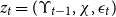 $z_t=(\Upsilon _{t-1},\chi ,\epsilon _t)$
, where
$z_t=(\Upsilon _{t-1},\chi ,\epsilon _t)$
, where
 $z=(\Upsilon ,0,0)$
identifies the expansion point. The stability of our model follows the concept of mean-square stability outlined by Farmer et al. (Reference Farmer, Waggoner and Zha2011).
$z=(\Upsilon ,0,0)$
identifies the expansion point. The stability of our model follows the concept of mean-square stability outlined by Farmer et al. (Reference Farmer, Waggoner and Zha2011).
The above law of motion is combined with the observation equations—in Appendix D—to build a state space system. Given the data presented in Appendix E, the model is estimated with Bayesian methods to construct the parameters’ posterior distribution. The likelihood is computed with a variant of the Kim filter, originally proposed by Kim and Nelson (Reference Kim and Nelson1999).Footnote 20 The states’ probabilities are extracted using the Hamilton (Reference Hamilton1989) filter. The obtained likelihood is combined with a prior distribution for the parameters, forming the posterior kernel. We first find the posterior modes and then use them as starting points to initialise the Metropolis-Hastings algorithm to sample from the posterior distribution. We generate two chains, each consisting of 100,000 draws (1 every ten draws is saved), with a burn-in period of 15% of them. The scale parameter is set to obtain an acceptance rate of around 35%. Model diagnostics are presented in Appendix G.
Importantly, we do not impose ex-ante restrictions on the combinations of monetary and fiscal behaviours in
 $\xi ^p_t$
. The estimation allows all the pairings of policy mix states (AM/PF; PM/AF; AM/AF; PM/PF). For each candidate parameter vector, the model is solved around the regime-specific steady state. We then check existence and uniqueness conditions for the local linear rational expectations solution. Parameter draws (and the associated regimes’ combinations) that fail to yield a valid, determinate solution produce an undefined or negligible likelihood and thus attract effectively zero posterior weight in the estimation. Consequently, the posterior distribution concentrates only on those regime-combinations that are both theoretically admissible (existence/uniqueness) and empirically supported by the data. In our sample, the estimation therefore selects two determinate policy mixes (AM/PF and PM/AF): other combinations either produce indeterminacy/non-existence at relevant parameter values or are unsupported by the data.
$\xi ^p_t$
. The estimation allows all the pairings of policy mix states (AM/PF; PM/AF; AM/AF; PM/PF). For each candidate parameter vector, the model is solved around the regime-specific steady state. We then check existence and uniqueness conditions for the local linear rational expectations solution. Parameter draws (and the associated regimes’ combinations) that fail to yield a valid, determinate solution produce an undefined or negligible likelihood and thus attract effectively zero posterior weight in the estimation. Consequently, the posterior distribution concentrates only on those regime-combinations that are both theoretically admissible (existence/uniqueness) and empirically supported by the data. In our sample, the estimation therefore selects two determinate policy mixes (AM/PF and PM/AF): other combinations either produce indeterminacy/non-existence at relevant parameter values or are unsupported by the data.
5. Monetary/fiscal policy mix regimes
The model is estimated using eight post-war time series for France and Italy, collected at an annual frequency, spanning samples 1955–2019 and 1950–2019 respectively. These include real GDP growth, domestic GDP deflator inflation, euro-wide consumer price inflation, short-term interest rate, and four fiscal variables expressed as GDP ratios: government debt, tax revenues, government expenditure, and government purchases. Appendix E provides a detailed description of the data used and Appendix D presents their mapping in the model. We select France and Italy as two large countries in the EA with distinct histories of policy facts, both facing trade-offs in monetary-fiscal coordination. As Italy has always relatively had tighter fiscal constraints (as from higher debt ratios) whereas they shared similar monetary paths, the comparison tends to highlight the role of fiscal space for macroeconomic stability and sustainability.
Estimation. We first calibrate a set of parameters. For both economies, we set the discount factor
 $\beta$
to 0.9804, implying an annual real interest rate of 2%. We set the labour share at 66%,
$\beta$
to 0.9804, implying an annual real interest rate of 2%. We set the labour share at 66%,
 $\alpha =0.33$
, and the average maturity at five years, implying
$\alpha =0.33$
, and the average maturity at five years, implying
 $\rho =0.816$
. To separate the short- from the long-term component of government expenditure, we fix
$\rho =0.816$
. To separate the short- from the long-term component of government expenditure, we fix
 $\rho _{e^L}=0.99$
, and
$\rho _{e^L}=0.99$
, and
 $\sigma _{e^L}=0.001$
, in line with Bianchi and Ilut (Reference Bianchi and Ilut2017). Finally, we calibrate the steady-state value of inflation for the rest of the EA to its empirical average value,
$\sigma _{e^L}=0.001$
, in line with Bianchi and Ilut (Reference Bianchi and Ilut2017). Finally, we calibrate the steady-state value of inflation for the rest of the EA to its empirical average value,
 $\Pi _{rEA}=1.1\%$
for France and
$\Pi _{rEA}=1.1\%$
for France and
 $\Pi _{rEA}=1.3\%$
for Italy.
$\Pi _{rEA}=1.3\%$
for Italy.
The remaining parameters are estimated using Bayesian priors and MS techniques to capture changes in policy mix regimes. Table 1 reports the prior distributions and posterior estimates for both economies. The priors for the steady-state parameters are centred at the country-specific empirical average values. The remaining priors follow Bianchi and Melosi (Reference Bianchi and Melosi2017), where those for consumption habit, the slope of the Phillips curve, and inflation indexation are adjusted from them quarterly to the lower annual frequency. The priors on shocks’ persistence and standard deviations are relatively loose and uninformative.
The posterior estimates are displayed by country. For both countries, the responses of interest rates to inflation,
 $\psi _{\pi }$
, are above 1 in the AM regime and below 1 in PM. Differences are less striking for the response to output,
$\psi _{\pi }$
, are above 1 in the AM regime and below 1 in PM. Differences are less striking for the response to output,
 $\psi _{y}$
, and even less for Italy. Regarding the response of taxes to debt,
$\psi _{y}$
, and even less for Italy. Regarding the response of taxes to debt,
 $\delta _b$
, we fix its value in the AF regime at 0, namely, imposing no responses of taxes on debt-to-GDP deviations. Instead, we estimate its value in the alternative regime. For both economies, the responses to debt are higher than the threshold value used to identify passive fiscal behaviour (
$\delta _b$
, we fix its value in the AF regime at 0, namely, imposing no responses of taxes on debt-to-GDP deviations. Instead, we estimate its value in the alternative regime. For both economies, the responses to debt are higher than the threshold value used to identify passive fiscal behaviour (
 $\beta ^{-1}-1=0.0171$
), implying the occurrence of a PF regime. Under this regime, France adjusts taxes to debt more than Italy.
$\beta ^{-1}-1=0.0171$
), implying the occurrence of a PF regime. Under this regime, France adjusts taxes to debt more than Italy.
In Italy, expenditure acts procyclically, as from a positive estimated response of short-expenditure to the output gap (
 $\phi _y\gt 0$
). This result indicates that a procyclical discretionary policy fully offsets automatic stabilisers, in line with the empirical evidence presented by Aghion et al. (Reference Aghion, Hemous and Kharroubi2014) and Balassone and Kumar (Reference Balassone and Kumar2007). Expenditure is instead countercyclical in France (
$\phi _y\gt 0$
). This result indicates that a procyclical discretionary policy fully offsets automatic stabilisers, in line with the empirical evidence presented by Aghion et al. (Reference Aghion, Hemous and Kharroubi2014) and Balassone and Kumar (Reference Balassone and Kumar2007). Expenditure is instead countercyclical in France (
 $\phi _y\lt 0$
), decreasing in booms and increasing in downturns.
$\phi _y\lt 0$
), decreasing in booms and increasing in downturns.
In line with these findings, Italy has an higher steady state debt-to-GDP ratio, partly from the cumulation of an higher steady state expenditure-to-GDP ratio and lower taxes-to-GDP ratio. Italy also features higher macroeconomic volatility and lower long-run growth.

Figure 3. Posterior probabilities of monetary/fiscal policy regimes. The figure shows the states’ smoothed probabilities evaluated at the posterior modes of the model, associated with regimes {[M], [F], [E]}, for the two model economies.
Policy mix regimes. Active and passive policy behaviours combine into three policy mix scenarios: an AM/PF regime; a PM/AF regime; an ELB monetary-active fiscal regime (ELB/AF). To link regime changes to historical accounts of the interaction of the monetary and fiscal authorities in France and Italy, Figure 3 plots the smoothed probabilities assigned to the three policy mix regimes, as defined in Section 4.
The three policy mix regions highlight a clear evolution in the relationship between fiscal and monetary policy over the decades, closely mirroring the historical events presented in Section 2: a PM/AF regime covering the first period of sustained growth, high inflation, and low fiscal imbalances; an AM/PF regime describing the switch to the monetary union framework, with a rigid separation between the ECB controlling inflation and fiscal policies committed to debt adjustments; a regime of constrained monetary policy combined with active fiscal behaviour. The latter can be interpreted as a special case of PM/AF regime.
The timing of regime shifts differs in the two countries to reflect substantial differences in their historical events, varying economic structures, and policy transmission mechanisms. From 1955 to the early 1990s, France operated under a Passive Monetary/Active Fiscal (PM/AF) regime, where the fiscal authority played a leading role. This period coincided with the country’s steady economic and industrial development, marked by policies of economic dirigisme (1955–75). Key historical events, such as the devaluations in 1958 and 1969, were instrumental in boosting growth and enhancing competitiveness, albeit at the cost of economic overheating and high inflation. Despite these challenges, primary deficits were managed in a way that maintained a low debt-to-GDP ratio, thus stimulating the economy and creating additional fiscal space for sustainability.
During this era, even efforts to curb inflation, like the Plan Barre in 1976, still operated within the PM/AF framework, where monetary policy was subordinated to fiscal needs. The shift began in 1983 when France started to peg the franc to the Deutsche Mark under the ERM, marking a significant transition in monetary policy (Smets, Reference Smets2007). This external anchor helped restore disinflation and exchange rate stability by 1986–87.
As France moved towards European integration, the Mitterrand fiscal consolidation plans of the 1980s accommodated the new monetary discipline, as evidenced by Aldama and Creel (Reference Aldama and Creel2020).Footnote 21 This marked the transition to an Active Monetary/Passive Fiscal (AM/PF) regime, aligning with the institutional framework designed by the euro membership. The ECB became the leading authority, acting on its price stability mandate, while fiscal policy was increasingly constrained by the requirements of the Stability and Growth Pact (SGP), which enforced fiscal discipline and prohibited excessive deficits. This period was characterised by low interest rates, sluggish growth, and increasing debt accumulation, setting the stage for the challenges that would follow.
This policy mix persisted until the Global Financial Crisis, which required a significant shift in strategy. Faced with a severe contraction in real economic activity, policymakers were forced to adopt extraordinary monetary policy measures. The ECB aggressively cut interest rates to the ELB, while the fiscal authority, abandoning its focus on debt stabilisation, shifted towards economic stimulus to combat the recession. This shift marked a return to a regime of active fiscal behaviour under constrained monetary policy, which can be interpreted as an ELB/Active Fiscal (ELB/AF) regime. The need for fiscal expansion to stimulate demand and escape the deflationary trap was paramount during this period (Sims, Reference Sims2016), resulting in low real rates, deflationary pressures, and rising debt ratios.
The results for Italy confirm the low-frequency relationship between fiscal stances and inflation found in a time-varying reduced-form VAR model by Kliem et al. (Reference Kliem, Kriwoluzky and Suarez2016).Footnote 22 During the 1970s, when the Bank of Italy was obligated to monetise government debt, the country operated under a Passive Monetary/Active Fiscal (PM/AF) regime, which contributed to high inflation and fiscal imbalances. This aligns with historical events with initial low fiscal deficits but a favourable expansion determining low real rates and debt ratios. Later, the central bank’s lack of independence led to significant budget deficits and the creation of a monetary base tied to Treasury financing. The transition to an Active Monetary/Passive Fiscal (AM/PF) regime began a few years later with respect to France, with the 1981 divorce between the Bank of Italy and the Treasury, marking a pivotal change in the relationship between monetary and fiscal authorities (Kliem et al. Reference Kliem, Kriwoluzky and Sarferaz2016). However, as noted by Fratianni and Spinelli (Reference Fratianni and Spinelli1997), this shift did not immediately result in lower inflation rates, as the fiscal authorities initially resisted fully supporting the central bank’s gradual move towards independence (Bartoletto et al. Reference Bartoletto, Chiarini and Marzano2013).
The process of establishing full central bank independence took over a decade, culminating in 1992 when, in compliance with the Maastricht Treaty, Italy formally abolished the law requiring the Bank of Italy to act as a residual buyer at treasury bill auctions. This institutional change coincided with a significant shift in fiscal policy (Paesani and Piga, Reference Paesani and Piga2002; Balassone et al. Reference Balassone, Francese and Pace2013), evidenced by the Amato and Dini reforms in 1992 and 1995, respectively. They were part of Italy’s efforts to align its public finances with the criteria necessary for joining the EMU in 1997.
Throughout the period leading up to the global financial crisis, Italy’s economic policy was characterised by inflation targeting, underpinned by fiscal discipline, resulting in low inflation, high real rates, and peaking debt-to-GDP ratios. By 2009, policy rates had reached the ELB, and fiscal austerity measures were intensified, particularly under the Berlusconi government in 2011 and the Monti government in 2012, as market pressures mounted. The subsequent shift in the policy mix in 2012 led to a reversal towards active fiscal behaviour, which, in the context of the global crisis, contributed to a vicious cycle of deflation, output contraction, and escalating public debt.
5.1 Policy mix transmission
The propagation of shocks in our model depends on the policy regime in place and the state variables of the economy. Simulating fiscal, monetary, demand, and supply shocks in the two economies, as shown in Figure 4 and 5, highlight relevant dynamic features within and across regimes. Specifically, impulse responses are computed conditionally for each policy regime prevailing over the entire horizon, but they continue to reflect the possibility of regime changes. They illustrate how regime-specific dynamics differ markedly between France and Italy, with fiscal space playing a key role in shaping responses. Then, in Appendix H, we compare the estimated responses to those generated under a benchmark regime-specific calibration for the policy rules (Kim, Reference Kim2003).
In France, a monetary contraction is recessionary and generates increases in the cost of debt (real rates) through sticky prices, accelerating its long-run accumulation under both regimes. This generates inflation, followed by a lagged expansionary effect, when the fiscal authority is leading. Therefore, the monetary policy shock backfires, as predicted by the stepping-on-a-rake mechanism (Sims, Reference Sims2011), namely, following an interest rate increase, spending increases due to a positive wealth effect, which then increases output and inflation. In contrast, when the economy is in the AM/PF regime, standard transmission applies: a monetary contraction leads to a decrease in output and inflation.

Figure 4. Regime-dependent impulse responses to macroeconomic shocks—France. Responses are conditional to the regime in place, implying that it will prevail over the entire simulation window. The displayed impulse responses are simulated over a monetary policy shock (
 $\epsilon ^{R}_t$
), a shock to the long-term expenditure (
$\epsilon ^{R}_t$
), a shock to the long-term expenditure (
 $\epsilon ^{e^L}_t$
), a preference shock (
$\epsilon ^{e^L}_t$
), a preference shock (
 $\epsilon ^{d}_t$
), and a mark-up shock (
$\epsilon ^{d}_t$
), and a mark-up shock (
 $\epsilon ^{\mu }_t$
). The blue solid line corresponds to the PM/AF regime, the red dashed one to the AM/PF regime. Results refer to the estimates on French data. The simulation horizon is 20 years.
$\epsilon ^{\mu }_t$
). The blue solid line corresponds to the PM/AF regime, the red dashed one to the AM/PF regime. Results refer to the estimates on French data. The simulation horizon is 20 years.

Figure 5. Regime-dependent impulse responses to macroeconomic shocks—Italy. Responses are conditional to the regime in place, implying that it will prevail over the entire simulation window. The displayed impulse responses are simulated over a monetary policy shock (
 $\epsilon ^{R}_t$
), a shock to the long-term expenditure (
$\epsilon ^{R}_t$
), a shock to the long-term expenditure (
 $\epsilon ^{e^L}_t$
), a preference shock (
$\epsilon ^{e^L}_t$
), a preference shock (
 $\epsilon ^{d}_t$
), and a mark-up shock (
$\epsilon ^{d}_t$
), and a mark-up shock (
 $\epsilon ^{\mu }_t$
). The blue solid line corresponds to the PM/AF regime, the red dashed one to the AM/PF regime. Results refer to the estimates on Italian data. The simulation horizon is 20 years.
$\epsilon ^{\mu }_t$
). The blue solid line corresponds to the PM/AF regime, the red dashed one to the AM/PF regime. Results refer to the estimates on Italian data. The simulation horizon is 20 years.
An expansionary long-term expenditure shock, financed by nominal debt, triggers expansion, increasing output, and inflation. Under the PM/AF regime, the shock is only partially controlled by policy rates, which respond only weakly to higher inflation allowing the latter to revalue debt downward, generating a sustained decline in real rates and the debt ratio. Indeed, the FTPL predicts that a positive fiscal shock, under no prospect that future taxes will rise, leads to a positive wealth effect, which increases spending and thereby inflation and output. The revaluation of government debt stimulate further aggregate demand and real growth, ultimately generating a persistent drop in the debt-to-GDP ratio. Under AM/PF, the expectation of future fiscal consolidation largely offsets the expansionary effects of the shock, producing muted responses in GDP and inflation and leading instead to debt accumulation.Footnote 23 This is a conventional Ricardian equivalence result.
A positive preference shock generates real economic expansion and an initial increase in inflation under both regimes, in line with the standard predictions of new Keynesian models. However, under PM/AF the induced drop in the fiscal burden and the milder increase in real rates are deflationary. The markup shock acts as a shock to inflation, and its effect on output differs across regimes. A drop in output is registered under the AM/PF regime after a few periods, whereas under the PM/AF regime, this happens only with some more delay. Simulated scenarios on agents’ beliefs prove that this initial expansion features the PM/AF regime and the AM/PF regime only when agents attach some probabilities to switch back to the PM/AF regime. Moreover, in AM/PF, interest rates adjust more, and real rates decrease. The fiscal burden first decreases but converges to zero over the long run. Under the PM/AF regime, the positive increase in output and the deeper drop in real rates explain the larger and more permanent contraction in the debt ratio.
Italy’s responses differ in both magnitude and persistence. Unlike in France, expectations of the stepping-on-a-rake effect already matter in the AM/PF regime: monetary policy shocks increase real rates and future debt, thereby increasing inflation through the anticipated transition back to the PM/AF regime. Moreover, differently from France, the monetary contraction in Italy under the PM/AF regime turns into an upward output trend after 2 years, as expectations of missing fiscal adjustments justify higher demand, output, and spending. However, fiscal shocks are more persistent and destabilising in the PM/AF regime. Indeed, procyclicality in discretionary expenditure amplifies output and price fluctuations, eroding fiscal balances and contributing to further debt accumulation more than under AM/PF. Preference shocks raise GDP and prices in both regimes. As from procyclical fiscal policy, expenditure increases, inflating debt evaluations after a few periods in both regimes despite declines in real rates. The opposite happens in France where lower expenditure—acting countercyclically—supports debt declines, dominating increasing real rates. Finally, a supply-side markup shock in Italy triggers a sharper and more immediate recession than in France, real rates fall under both regimes, and in PM/AF debt declines persistently via consolidation policies, albeit at the cost of deeper recession.
Overall, the cross-country comparison shows that France’s larger fiscal space allows countercyclical short-term expenditure responses that dampen volatility and smooth debt adjustments, whereas Italy’s constrained fiscal capacity forces procyclical adjustments, amplifying shocks and undermining stability. This mechanism operates across shock types—not only for fiscal disturbances but also for monetary, demand, and supply shocks—explaining the divergences in shocks’ transmission across policy mix regimes. Importantly, while in France the degree of fiscal sustainability—as reflected in the debt-to-GDP responses—depends strongly on the prevailing policy mix, in Italy debt tends to rise following all shocks except a recessionary markup shock, underscoring the structural weight of fiscal constraints in shaping outcomes.

Figure 6. Regime-dependent impulse responses under policy credibility scenarios—France. The figure compares the impulse responses under the estimated PM/AF regime for France with the simulated PM/AF responses of a confidence and a fully credible scenario. A confidence scenario is generated by increasing the probability to go from the PM/AF to the AM/PF regime from 0.007 to 0.105, and decreasing the probability to go from AM/PF to PM/AF from 0.017118 to 0.001. A credible scenario is simulated by increasing the probability to go from PM/AF to AM/PF to 1 and decrease the probability to go from AM/PF to PM/AF to 0. The displayed impulse responses are simulated over a monetary policy shock (
 $\epsilon ^{R}_t$
), a shock to the long-term expenditure (
$\epsilon ^{R}_t$
), a shock to the long-term expenditure (
 $\epsilon ^{e^L}_t$
), a preference shock (
$\epsilon ^{e^L}_t$
), a preference shock (
 $\epsilon ^{d}_t$
), and a mark-up shock (
$\epsilon ^{d}_t$
), and a mark-up shock (
 $\epsilon ^{\mu }_t$
). The simulation horizon is 20 years.
$\epsilon ^{\mu }_t$
). The simulation horizon is 20 years.

Figure 7. Regime-dependent impulse responses under policy credibility scenarios—Italy. The figure compares the impulse responses under the estimated PM/AF regime for Italy with the simulated PM/AF responses of a confidence and a fully credible scenario. A confidence scenario is generated by increasing the probability to go from the PM/AF to the AM/PF regime from 0.003 to 0.04, and decreasing the probability to go from AM/PF to PM/AF from 0.012 to 0.001. A credible scenario is simulated by increasing the probability to go from PM/AF to AM/PF to 1 and decrease the probability to go from AM/PF to PM/AF to 0. The displayed impulse responses are simulated over a monetary policy shock (
 $\epsilon ^{R}_t$
), a shock to the long-term expenditure (
$\epsilon ^{R}_t$
), a shock to the long-term expenditure (
 $\epsilon ^{e^L}_t$
), a preference shock (
$\epsilon ^{e^L}_t$
), a preference shock (
 $\epsilon ^{d}_t$
), and a mark-up shock (
$\epsilon ^{d}_t$
), and a mark-up shock (
 $\epsilon ^{\mu }_t$
). The simulation horizon is 20 years.
$\epsilon ^{\mu }_t$
). The simulation horizon is 20 years.
5.2 Belief scenarios about the policy mix
This section investigates how agents’ beliefs about the persistence of policy regimes influence the transmission of macroeconomic shocks. We compare the benchmark impulse responses - obtained from our estimation - with those generated under alternative assumptions about regime transition probabilities. By modifying these probabilities, we construct counterfactual scenarios that isolate the role of expectations about the future stance of the policy mix. Specifically, we examine how varying degrees of policy credibility and uncertainty—reflected in agents’ beliefs about the likelihood and duration of the AM/PF regime—shape how the economy behaves and responds to shocks in the current policy stance, whether in PM/AF or already in AM/PF.
Policy credibility scenarios. In a first set of simulations, we re-calibrate the transition matrix to reflect increasing degrees of credibility in the AM/PF regime, such as it is more likely to end up and remain in AM/PF. These simulations are in line with Bianchi and Ilut (Reference Bianchi and Ilut2017). Specifically, we define a confidence scenario, where we increase the probability of transitioning from PM/AF to AM/PF—from 0.007 to 0.11 for France, and from 0.003 to 0.04 for Italy—while simultaneously decreasing the probability of moving from AM/PF to PM/AF—from 0.02 to 0.001 for France, and from 0.012 to 0.001 for Italy. This setup reflects a moderate increase in agents’ belief that the policy mix will remain or revert to a credible AM/PF regime. In a more extreme scenario—the fully credible scenario—we impose full policy credibility by making the AM/PF regime absorbing. That is, the transition probability from PM/AF to AM/PF is set to 1, and any return from AM/PF to PM/AF is ruled out entirely. This scenario captures the case in which agents perceive the commitment to a sound policy mix as fully credible and irreversible.
All impulse responses are generated under the assumption that the economy is in the PM/AF regime, while agents form different expectations about the likelihood of transitioning to (and then remaining in) an AM/PF (Figure 6 and 7). This translates into a simulation on the role of expectations about AM/PF, given the PM/AF policy parameters. The model responses vary systematically with the credibility of such a policy shift. When agents expect the AM/PF regime to realise in the future with a higher probability, that is, when policy announcements effectively anchor expectations, in most cases they behave as if the policy change were already in place. Indeed, the stepping-on-a-rake effect associated with a more credible monetary policy contraction disappears in both countries. The same occurs in France for the expenditure shock, which leads to rising debt, and the preference shock, which turns inflationary. Given that in both scenarios we also assume a sharp reduction in the probability to exit AM/PF, in some cases the impulse responses reinforce the AM/PF dynamics.Footnote 24 In Italy, a credible commitment to exiting the PM/AF regime stabilises expectations toward the AM/PF, where the imbalances generated by procyclical expenditure remain.
Policy uncertainty scenarios. In a second set of simulations, we introduce agents’ uncertainty about the persistence of regime changes through calibrated differences in perceived transition probabilities. Following Bianchi and Melosi (Reference Bianchi and Melosi2014, Reference Bianchi and Melosi2018), agents are assumed to observe the regime in place and share common knowledge about the policy parameters and the transition matrix governing the coordination of fiscal and monetary policy. Uncertainty arises from agents’ inability to distinguish ex-ante whether the shift to AM/PF will be temporary or persistent. Hence, upon entering the AM/PF regime, agents behave as if they initially expect the change to be short-lived, and only gradually revise this belief as time in the regime lengthens and persistence becomes more credible.
This belief-perturbation approach preserves rational expectations while allowing us to examine how the perceived duration of a policy regime shapes the transmission of shocks.

Figure 8. Regime-dependent impulse responses under policy uncertainty scenarios—France. The figure compares the impulse responses under the estimated AM/PF regime for France with two simulated scenarios, where the transition matrix is expanded to include a short-lasting and a long-lasting AM/PF regime. A AM/PF-short scenario is generated by setting the probability to go from AM/PF temporary to AM/PF long-lasting to 0.01, and the probability to go from AM/PF temporary to the PM/AF regime to 0.49. A AM/PF-long scenario is simulated by setting the probability to go from AM/PF temporary to AM/PF long-lasting to 0.49 and the probability to go from AM/PF temporary to the PM/AF regime to 0.01. The impulse responses are simulated over a monetary policy shock (
 $\epsilon ^{R}_t$
), a shock to the long-term expenditure (
$\epsilon ^{R}_t$
), a shock to the long-term expenditure (
 $\epsilon ^{e^L}_t$
), a preference shock (
$\epsilon ^{e^L}_t$
), a preference shock (
 $\epsilon ^{d}_t$
), and a mark-up shock (
$\epsilon ^{d}_t$
), and a mark-up shock (
 $\epsilon ^{\mu }_t$
). The simulation horizon is 20 years.
$\epsilon ^{\mu }_t$
). The simulation horizon is 20 years.

Figure 9. Regime-dependent impulse responses under policy uncertainty scenarios—Italy. The figure compares the impulse responses under the estimated AM/PF regime for Italy with two simulated scenarios, where the transition matrix is expanded to include a short-lasting and a long-lasting AM/PF regime. A AM/PF-short scenario is generated by setting the probability to go from AM/PF temporary to AM/PF long-lasting to 0.01, and the probability to go from AM/PF temporary to the PM/AF regime to 0.49. A AM/PF-long scenario is simulated by setting the probability to go from AM/PF temporary to AM/PF long-lasting to 0.49 and the probability to go from AM/PF temporary to the PM/AF regime to 0.01. The impulse responses are simulated over a monetary policy shock (
 $\epsilon ^{R}_t$
), a shock to the long-term expenditure (
$\epsilon ^{R}_t$
), a shock to the long-term expenditure (
 $\epsilon ^{e^L}_t$
), a preference shock (
$\epsilon ^{e^L}_t$
), a preference shock (
 $\epsilon ^{d}_t$
), and a mark-up shock (
$\epsilon ^{d}_t$
), and a mark-up shock (
 $\epsilon ^{\mu }_t$
). The simulation horizon is 20 years.
$\epsilon ^{\mu }_t$
). The simulation horizon is 20 years.
Formally, these simulations rely on three regimes: a PM/AF regime; a short-lived AM/PF regime; a long-lasting AM/PF regime. The two AM/PF regimes share the same policy parameters but differ in their persistence, captured by alternative calibrations of the transition probabilities in the perceived law of motion.
We compare our benchmark impulse responses under the AM/PF regime with two alternative belief scenarios, where the AM/PF regime is perceived as either temporary or long-lasting. In a first scenario, labelled AM/PF-short, the transition matrix is set such that the probability of moving from the temporary AM/PF regime to the long-lasting AM/PF regime is 0.01, while the probability of reverting to the PM/AF regime is 0.49. In a second scenario, denoted AM/PF-long, we assume the probability of transitioning from the temporary to the long-lasting AM/PF regime is 0.49, while the probability of returning to the PM/AF regime is only 0.01. These calibrated probabilities serve as a reduced-form representation of uncertainty about regime duration.
For France, Figure 8 shows that when agents expect the AM/PF regime to be short-lived—anticipating a rapid reversion to the PM/AF regime—the monetary shock becomes inflationary, the expenditure shock reduces debt, and the preference shock is deflationary. These results reflect a muted adjustment of expectations: agents do not fully internalise the regime shift when they perceive it as transitory. Thus, the dynamics converge to those observed under a PM/AF regime, in line with Bianchi and Melosi (Reference Bianchi and Melosi2014), who document a similar pattern for fiscal shocks.
When the shift to the AM/PF regime is instead perceived as more persistent, the relevant dynamics of the AM/PF regime are reinforced, especially under an expenditure shock. Figure 9 confirms these results for Italy. Importantly, the AM/PF-long scenario removes the inflationary effects derived from the anticipated transition to the PM/AF in the face of a monetary contraction, leading to a deeper recession. Moreover, while in France the AM/PF-long explains higher debt accumulation, in Italy the most amplifying scenario is the AM/PF-short, as it entails a stronger procyclical expansion in expenditure, higher inflation, and faster debt growth. This result clarifies how Italian debt dynamics tend to depend more on fiscal space than on the prevailing policy mix regime.
6. Policy recommendations
While our analysis primarily provides a positive assessment of the differentials in inflation and fiscal dynamics in France and Italy, several policy recommendations can be derived. In particular, inspired by the recent work by Beyer et al. (Reference Beyer, Duttagupta, Fotiou, Honjo, Horton, Jakab, Nguyen, Portillo, Lindé, Suphaphiphat and Zeng2023), where they highlight the benefits of synchronised and union-wide fiscal measures as a complement to monetary policy in addressing inflation, our paper provides support to the benefits of coordinated monetary/fiscal strategies.Footnote 25 In particular:
-
• Italy, characterised by higher debt and procyclical fiscal behaviour in our analysis, aligns with a high-debt country in the Beyer et al. (Reference Beyer, Duttagupta, Fotiou, Honjo, Horton, Jakab, Nguyen, Portillo, Lindé, Suphaphiphat and Zeng2023)’s model. They show that when only high-debt countries consolidate, these countries bear disproportionate output costs, while all members benefit from reduced interest rates-implying a coordination failure. The estimated pro-cyclical fiscal behaviour in Italy confirms the deepened recessionary dynamics derived from fiscal consolidation.
-
• France, which showed relatively milder inflationary pressures and more stable fiscal conduct in our results, would relatively correspond to a low-debt country group that, in their setup, benefits from positive cross-border spillovers when others consolidate.
In light of this, the presence of asymmetries in inflation dynamics and fiscal responses supports the normative case for a shared fiscal response to EA-wide inflation shocks. Without coordination, high-debt countries like Italy face amplified adjustment costs, which may reduce policy effectiveness. A central fiscal capacity would internalise cross-country spillovers and align national incentives.
7. Conclusions
This study examines debt sustainability and inflation dynamics in Italy and France—two economies with a history of monetary independence, Treasury-Central Bank agreements, and fiscal instability. Using post-war data, we estimate a DSGE model with MS policy rules for tax revenues and nominal interest rates, capturing monetary-fiscal interactions, EMU transition, and ELB constraints.
Estimated policy regimes reveal distinct macroeconomic narratives. Since the 1950s, both countries followed a PM/AF regime, marked by fiscal-driven inflation and debt monetisation. The transition to AM/PF in the 1990s, driven by European integration, reduced inflation but increased debt burdens, with France shifting earlier due to ERM-induced fiscal discipline. Italy’s procyclical fiscal policy amplified volatility and constrained growth. Since 2009, the ELB limited monetary policy, prompting fiscal expansion in France, while Italy’s austerity delayed adjustment.
Simulations show that PM/AF stabilises debt but increases price volatility, while AM/PF curbs inflation at the cost of higher debt burdens. A key driver of these regime-specific dynamics is fiscal space: Italy’s persistently high debt ratios constrain fiscal policy, fostering procyclical adjustments that amplify output volatility and undermine stability, whereas France’s larger fiscal space enables countercyclical responses and greater scope for policy coordination. Policy credibility also shapes regime shifts, as agents anticipating changes in the policy mix adjust behaviour in ways that reinforce transitions. Finally, uncertainty over regime duration slows agents’ adjustments, influencing the speed and effectiveness of policy transmission.
Acknowledgements
We thank Pierpaolo Benigno, Huixin Bi, Giovanni Di Bartolomeo, Marco Di Pietro, Christophe Kamps, Francesco Giuli, Eric Leeper, Nadine Leiner Killinger, Marcello Messori, Alessandro Notarpietro, Joseph Plasmans, Massimiliano Tancioni, Patrizio Tirelli, and participants to the WGEM expert group on monetary and fiscal interaction, for useful discussions and suggestions. The views expressed are those of the authors and do not necessarily reflect those of the European Central Bank.
Appendix A. Equilibrium conditions
The model is characterised by the following set of equilibrium equations, in the endogenous variables
 $\{\hat {c}_t, R_t^m, R_t,P^m_t, \pi _t, \varphi _t, h_t, \hat {y}_t, b_t, \tau _t, e_t, e^S_t, \chi _t, g_t, \hat {y}_t^n, v_t\}$
and exogenous variables
$\{\hat {c}_t, R_t^m, R_t,P^m_t, \pi _t, \varphi _t, h_t, \hat {y}_t, b_t, \tau _t, e_t, e^S_t, \chi _t, g_t, \hat {y}_t^n, v_t\}$
and exogenous variables
 $\{a_t, d_t, \mu _t, tp_t, e^L_t, \Pi _{rEA,t}\}$
. Detrended variables (normalised by the level of aggregate TFP) are defined as
$\{a_t, d_t, \mu _t, tp_t, e^L_t, \Pi _{rEA,t}\}$
. Detrended variables (normalised by the level of aggregate TFP) are defined as
 $\hat {X}_t$
.
$\hat {X}_t$
.
-
1. Euler equation:
 $1 = \beta \mathbb{E}_t \Bigg \{ e^{d_{t+1}-d_t} \frac {\hat {c}_t - \Phi \hat {c}_{t-1}e^{-(\gamma +a_{t})}}{\hat {c}_{t+1} - \Phi \hat {c}_{t}e^{-(\gamma +a_{t+1})}} e^{-(\gamma +a_{t+1})} \frac { R^m_{t+1}}{\Pi _{t+1}}\Bigg \}$
-
2. Long-term return:
$R_t^m = \frac {1+\rho P^m_{t}}{P_{t-1}^m}$
-
3. Arbitrage condition:
$ R_t = \mathbb{E}_t [R_{t+1}^m]$
-
4. Real marginal costs:
$\varphi _t = \big [\hat {c}_t - \Phi \hat {c}_{t-1} e^{-(\gamma +a_t)} \big ] \frac {h_t^{\alpha }}{1-\alpha }$
-
5. Production function:
$\hat {y}_t = h_t^{1-\alpha }$
-
6. Phillips Curve:
$\frac {1}{\nu _t}\big (1-\varphi _t(1-\alpha )\big ) = 1 - \psi \bigg ( \Pi _t - \frac {\Pi _{t-1}^\iota }{\Pi ^{\iota -1}}\bigg ) \Pi _t - \frac {\psi }{2} \bigg (\Pi _t - \frac {\Pi _{t-1}^\iota }{\Pi ^{\iota -1}} \bigg )^2 \frac {\nu _t -1}{\nu _t}\ \ \ \ $
$+ \beta \mathbb{E}_t \Bigg \{ \frac {\hat {c}_t - \Phi \hat {c}_{t-1}e^{-(\gamma +a_{t})}}{\hat {c}_{t+1} - \Phi \hat {c}_{t}e^{-(\gamma +a_{t+1})}} \psi \bigg (\Pi _{t+1} -\frac {\Pi _t^\iota }{\Pi ^{\iota -1}}\bigg ) \Pi _{t+1} \frac {\hat {y}_{t+1}}{\hat {y}_t}\Bigg \}$
-
7. Mark-up shock:
$\frac {\kappa }{1+\iota \beta } \log \bigg (\frac {1-\nu }{1-\nu _t} \bigg ) = \mu _t; \quad \mu _t =\rho _\mu \mu _{t-1}+\sigma _\mu \varepsilon ^\mu _t$
-
8. Taylor rule:
$\frac {R_t}{R} = \left (1-I_t^{ELB}\right )\left \{\bigg ( \frac {R_{t-1}}{R}\bigg )^{\rho _{R}} \Bigg [\bigg (\frac {\Pi _t^{\omega (I_t^{EA})}\Pi _{rEA,t}^{(1-\omega (I_t^{EA}))})}{\Pi }\bigg )^{\psi _{\pi ,\xi _t^p}} \bigg (\frac {Y_t}{Y_t^n}\bigg )^{y,\xi _t^p} \Bigg ]^{(1-\rho _{R})} e^{\sigma _{R}\varepsilon _{t}^{R}}\right \}$
$+I_t^{ELB}\left \{\left (\frac {R_{t-1}}{R}\right )^{\rho _{R,I}}(1/R)^{(1-\rho _{R,I})\psi _I}e^{\sigma _{I}\varepsilon _{t}^{R}}\right \}$
-
9. Budget constraint:
$b_t = b_{t-1} \frac {R_t^m}{\Pi _t} \frac {\hat {y}_{t-1}}{\hat {y}_{t}} e^{-(\gamma +a_t)} -\tau _t + e_t+tp_t$
-
10. Government purchases-to-expenditure:
$\frac {\chi _t}{\chi } = \bigg (\frac {\chi _{t-1}}{\chi }\bigg )^{\rho _{\chi }} e^{\sigma _{\chi }\varepsilon ^{\chi }_t}$
;
$\chi _t = \bigg ( 1-\frac {1}{g_t}\bigg )e_t^{-1}$
-
11. Government expenditure:
$e_t = e_t^S + e_t^L$
-
Short-term component:
$e_t^S = \rho _{e^S} e_{t-1}^S + (1-\rho _{e^S}) \bigg [ e^S + \phi _y \Big (\hat {y}_t - \hat {y}_t^n\Big )\bigg ] + \sigma _{e^S} \varepsilon _t^{e^S}$
-
Long-term component:
$e_t^L = \rho _{e^L} e_{t-1}^L + \sigma _{e^L} \varepsilon _t^{e^L}$
-
-
12. Tax rule:
$\tau _t = \rho _{\tau } \tau _{t-1} + (1-\rho _{\tau }) \left [ \tau + \delta _{b,\xi _t^{p}} (b_t - b) + \delta _{y} (y_t - y_t^n)\right ] \sigma _{\tau }\varepsilon _{t}^{\tau }$
-
13. Government Purchases:
$g_t \equiv \left (1-\frac {\hat {G}_{t}}{\hat {y}_t}\right )^{-1}$
-
14. Market clearing:
$1 = \frac {\hat {c}_t}{\hat {y_t}} + \frac {g_t-1}{g_t}$
-
15. Potential output:
$\hat {y}_t^n = \Bigg [ \frac {1-\nu _t}{\frac {\hat {y}_t^n}{g_t} - \Phi \frac {\hat {y}^n_{t-1}}{g_{t-1}} e^{-(\gamma + a_t)}}\Bigg ]^{\frac {1-\alpha }{\alpha }}$
-
16. TFP shock:
$a_t=\rho _{a}a_{t-1}+\sigma _{a}\varepsilon ^{a}_t$
-
17. Term premium shock:
$tp_t=\rho _{tp}tp_{t-1}+\sigma _{tp}\varepsilon ^{tp}_t$
-
18. Preference shock:
$d_t=\rho _{d}d_{t-1}+\sigma _{d}\varepsilon ^{d}_t$
-
19. Rest of euro area inflation shock:
$\Pi _{rEA,t}=\rho _{\Pi _{rEA}}\Pi _{rEA,t-1}+ \sigma _{\pi _{rEA}} \varepsilon _{t}^{\Pi _{rEA}}$


Appendix B. Steady-state system
Given initial data-based calibrations for
 $\Pi =\Pi ^{\star }; \quad g=g^{\star }; \quad b=b^{\star }; \quad \tau =\tau ^{\star }$
, the steady state of the model is characterised by the following set of equations:
$\Pi =\Pi ^{\star }; \quad g=g^{\star }; \quad b=b^{\star }; \quad \tau =\tau ^{\star }$
, the steady state of the model is characterised by the following set of equations:
 \begin{gather*}R^m = \frac {\Pi ^{\star }}{\beta }e^\gamma \\[4pt] P^m = \frac {1}{R^m - \rho } \\[4pt] R = R^m \\[4pt] \varphi = \frac {1-\nu }{1-\alpha }= \hat {c}(1-\Phi e^{-\gamma }) \frac {h^{\alpha }}{1-\alpha }\\[4pt] e = \left (1-\frac {1}{\beta } \right ) b^{\star } + \tau ^{\star }\\[4pt] e^S = e \end{gather*}
 \begin{gather*} \chi = \Big ( 1 - \frac {1}{g^{\star }}\Big ) e^{-1}\\[4pt] h = \varphi (1-\alpha ) \frac {g^{\star }}{1-\Phi e^{-\gamma }} \\[4pt] y = h^{1-\alpha } \\[4pt] c = \frac {y}{g^{\star }} \\[4pt] y^n = y\\[4pt] a=d=e^L=\mu =tp=\Pi _{rEA}=0 \end{gather*}
Appendix C. Linearised model
After de-trending the model, we linearise each equation around the steady state. We use the notation
 $\tilde {x}_t$
to indicate both linear deviations, (
$\tilde {x}_t$
to indicate both linear deviations, (
 $\tilde {x}_t=X_t-X$
), and percentage deviations from the steady-state level (
$\tilde {x}_t=X_t-X$
), and percentage deviations from the steady-state level (
 $\tilde {x}_t=\log (\frac {X_t}{X})$
, while for de-trended variables
$\tilde {x}_t=\log (\frac {X_t}{X})$
, while for de-trended variables
 $\tilde {x}_t=\log \Big (\frac {\hat {X}_t}{\hat {X}}\Big )=\log \Big (\frac {X_t}{A_t}\frac {A}{X}\Big )$
).
$\tilde {x}_t=\log \Big (\frac {\hat {X}_t}{\hat {X}}\Big )=\log \Big (\frac {X_t}{A_t}\frac {A}{X}\Big )$
).
-
1. IS curve:
\begin{align*} \tilde {y}_t=&\tilde {g}_t-\frac {1}{1+\Phi e^{-\gamma }}\mathbb{E}_t\{\tilde {g}_{t+1}\}+\frac {\Phi e^{-\gamma }}{1+\Phi e^{-\gamma }}(\tilde {y}_{t-1}-\tilde {g}_{t-1}-a_t)+ \\& -\frac {1-\Phi e^{-\gamma }}{1+\Phi e^{-\gamma }}(\tilde {R}_t-\mathbb{E}_t\{\tilde {\pi }_{t+1}\}-(1-\rho _d d_t))+\frac {1}{1+\Phi e^{-\gamma }}(\mathbb{E}_t\{\tilde {y}_{t+1}\}+\rho _a a_t) \end{align*}
-
2. Phillips Curve:
\begin{align*} \tilde {\pi }_t=&\frac {\kappa (1-\Phi e^{-\gamma })^{-1}}{1+\iota \beta }\Big [\Big (1+\frac {\alpha }{1-\alpha }(1-\Phi e^{-\gamma })\Big )\tilde {y}_t-\tilde {g}_t-\Phi e^{-\gamma }(\tilde {y}_{t-1}-\tilde {g}_{t-1}-a_t)\Big ]\\&+\frac {\iota }{1+\iota \beta }\tilde {\pi }_{t-1}+\frac {\beta }{1+\iota \beta }\mathbb{E}_t\{\tilde {\pi }_{t+1}\}+\mu _t \end{align*}
-
3. Taylor rule:
$\tilde {R}_t=\left (1-I_t^{ELB}\right )\left \{\rho _R\tilde {R}_{t-1}+(1-\rho _R)\left [\psi _{\pi ,\xi ^p_t} \left (\omega (I_t^{EA})\tilde {\pi }_t+(1-\omega (I_t^{EA}))\tilde {\pi }_{rEA,t}\right ) \right.\right.$
$ \left .+ \left.\psi _{y,\xi ^p_t}(\tilde {y}_t-\tilde {y}^n_t)\right ]+ \sigma _R \varepsilon ^R_{t}\right \}$
$+\,I_t^{ELB}\left \{\rho _{R,I}\tilde {R}_{t-1}-(1-\rho _{R,I})\psi _I \text{log}R+\sigma _I \varepsilon _{t}^{R}\right \}$
-
4. Government Purchases-to-expenditure:
$ \tilde {\chi }_t=\rho _\chi \tilde {\chi }_{t-1}+\sigma _\chi \epsilon ^{\chi }_t$
;
$ \tilde {\chi }_t=\frac {1}{g^{\star }-1}\tilde {g}_t-e^{-1}\tilde {e}_t$
-
5. Tax rule:
$\tilde {\tau }_t=\rho _{\tau } \tilde {\tau }_{t-1}+(1-\rho _{\tau })\big[\delta _{b,\xi _t^{p}}\tilde {b}_{t-1}+\delta _{y}(\tilde {y}_t-\tilde {y}_t^n)\big]+\sigma _\tau \epsilon ^{\tau }_t$
-
6. Debt:
$\tilde {b}^m_t=\beta ^{-1}\tilde {b}^m_{t-1}+b^m\beta ^{-1}\big(\tilde {R}^m_{t-1,t}-\tilde {y}_t+\tilde {y}_{t-1}-a_t-\tilde {\pi }_t\big)-\tilde {\tau }_t+\tilde {e}^S_t+e^L_t+tp_t$
-
7. Return on portfolio:
$\tilde {R}^m_{t,t+1}=R^{-1}\rho \tilde {P}^m_{t+1}-\tilde {P}^m_t$
-
8. No arbitrage:
$\tilde {R}_t=\mathbb{E}_t\{\tilde {R}^m_{t,t+1}\}$
-
9. Natural output:
$\Big [\frac {1}{1-\Phi e^{-\gamma }}+\frac {\alpha }{1-\alpha }\Big ]\tilde {y}_t^n=(1-\Phi e^{-\gamma })^{-1}\tilde {g}_t+\frac {\Phi e^{-\gamma }}{1-\Phi e^{-\gamma }}\big(\tilde {y}^n_{t-1}-\tilde {g}_{t-1}-a_t\big)$
-
10. Government expenditure:
$\tilde {e}_t=\tilde {e}^S_t+e^L_t$
-
Short-term component:
$\tilde {e}^S_t=\rho _{e^S}\tilde {e}^S_{t-1}+(1-\rho _{e^S})\phi _y\big(\tilde {y}_t-\tilde {y}^n_t\big)+\sigma _{e^S}\epsilon ^{e^S}_t$
-
Long-term component:
$e^L_t=\rho _{e^L}e^L_{t-1}+\sigma _{e^L}\epsilon ^{e^L}_t$
-
-
11. Term premium shock:
$tp_t=\rho _{tp}tp_{t-1}+\sigma _{tp}\epsilon ^{tp}_t$
-
12. Technology shock:
$a_t=\rho _{a}a_{t-1}+\sigma _{a}\epsilon ^{a}_t$
-
13. Preference shock:
$d_t=\rho _{d}d_{t-1}+\sigma _{d}\epsilon ^{d}_t$
-
14. Mark-up shock:
$\mu _t=\rho _{\mu }\mu _{t-1}+\sigma _{\mu }\epsilon ^{\mu }_t$
-
15. Rest of euro area Inflation shock:
$\tilde {\pi }_{rEA,t}=\rho _{\pi _{rEA}}\tilde {\pi }_{rEA,t-1}+ \sigma _{\pi _{rEA}} \varepsilon _{t}^{\pi _{rEA}}$


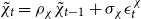


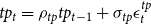


Appendix D. Observation equations
The vector of model solutions
 $S_t$
is combined with the following system of observation equations:
$S_t$
is combined with the following system of observation equations:
 \begin{align} X_t=D+ZS_t \end{align}
where
 $X_t=[\Delta \log (y_t^{\text{obs}}),\,\pi _t^{\text{obs}},\,R_t^{\text{obs}},\,b_t^{\text{obs}},\,\log (g_t^{\text{obs}}),\,\tau _t^{\text{obs}},\,e_t^{\text{obs}}]^{'}$
contains the observables,
$X_t=[\Delta \log (y_t^{\text{obs}}),\,\pi _t^{\text{obs}},\,R_t^{\text{obs}},\,b_t^{\text{obs}},\,\log (g_t^{\text{obs}}),\,\tau _t^{\text{obs}},\,e_t^{\text{obs}}]^{'}$
contains the observables,
 $D$
is the vector of constants, and
$D$
is the vector of constants, and
 $Z_t$
provides the mapping between the model’s solution and the data. The system of observation equations reads as follows:
$Z_t$
provides the mapping between the model’s solution and the data. The system of observation equations reads as follows:
 \begin{gather*} \Delta \log (y_t^{\text{obs}})= \gamma +a_t+\tilde {y}_t-\tilde {y}_{t-1}\\[4pt] \log (\pi _t^{\text{obs}})=\log \left (\frac {P^{\text{obs}}_t}{P^{\text{obs}}_{t-1}}\right )=\log (\Pi ^{\star })+\tilde {\pi }_t\\[4pt] \log (\pi _{rEA,t}^{\text{obs}})=\log (\Pi _{rEA}^{\star })+\tilde {\pi }_{rEA,t}\\[4pt] R_t^{\text{obs}}=\left (\log (\Pi ^{\star })+\left (\frac {e^{\gamma }}{\beta }-1\right )\right )+\tilde {R}_t\\[4pt] b_t^{\text{obs}}=b^{\star }+\tilde {b}_t\\[4pt] \log (g_t^{\text{obs}})=\log (g^{\star })+\tilde {g}_t\\[4pt] \tau _t^{\text{obs}}=\tau ^{\star }+\tilde {\tau }_t\\[4pt] e_t^{\text{obs}}=e+\tilde {e}_t \end{gather*}
where the percentage deviation of the de-trended output from its steady state is
 $\tilde {y}_t=\log \left (\frac {Y_t^{\text{obs}}}{A_t}\frac {y}{A}\right )$
and the percentage deviations for inflation, government purchases, and interest rates are
$\tilde {y}_t=\log \left (\frac {Y_t^{\text{obs}}}{A_t}\frac {y}{A}\right )$
and the percentage deviations for inflation, government purchases, and interest rates are
 $\tilde {\pi }_t=\log \left (\frac {\Pi _t^{\text{obs}}}{\Pi ^{\star }}\right )$
,
$\tilde {\pi }_t=\log \left (\frac {\Pi _t^{\text{obs}}}{\Pi ^{\star }}\right )$
,
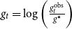 $g_t=\log \left (\frac {g_t^{\text{obs}}}{g^{\star }}\right )$
with
$g_t=\log \left (\frac {g_t^{\text{obs}}}{g^{\star }}\right )$
with
 $g_t^{\text{obs}}=(1-G_t^{\text{obs}}/Y_t^{\text{obs}})^{-1}$
,
$g_t^{\text{obs}}=(1-G_t^{\text{obs}}/Y_t^{\text{obs}})^{-1}$
,
 $\tilde {R}_t=\text{log}\left (\frac {R_t^{\text{obs}}}{R}\right )$
. For the variables normalised with respect to GDP, the linear deviations are
$\tilde {R}_t=\text{log}\left (\frac {R_t^{\text{obs}}}{R}\right )$
. For the variables normalised with respect to GDP, the linear deviations are
 $\tilde {\tau }_t=\tau _t^{\text{obs}}-\tau ^{\star }$
,
$\tilde {\tau }_t=\tau _t^{\text{obs}}-\tau ^{\star }$
,
 $\tilde {b}_t=b_t^{\text{obs}}-b^{\star }$
, and
$\tilde {b}_t=b_t^{\text{obs}}-b^{\star }$
, and
 $\tilde {e}_t=e_t^{\text{obs}}-e$
.
$\tilde {e}_t=e_t^{\text{obs}}-e$
.
Appendix E. Data
Country: France, Italy.
-
•
$Y_t^{\text{obs}}$
: Real GDP. France: Database: National accounts. Source: INSEE. Webpage: https://insee.fr/en/information/2868584#titre-bloc-1 Italy: Database: Baffigi (Reference Baffigi2013). Source: Bank of Italy, ISTAT. Webpage: https://www.bancaditalia.it/pubblicazioni/collana-storica/pil-storia-italia/index.html
-
•
$\Pi _t^{\text{obs}}$
: GDP deflator inflation. France: Database: National accounts. Source: INSEE. Italy: Database: Baffigi (Reference Baffigi2013). Source: Bank of Italy; ISTAT. -
•
$R_t^{\text{obs}}$
: short-term nominal interest rate. France: Call Money/Interbank Rate: Less than 24 Hours. Database: Main Economic Indicators. Source: OECD. Webpage: http://stats.oecd.org Italy: Official Discount rate (1950–1992); three-month money market rate (1993–2018). Database: Historical Tables. Monetary and Financial Indicators (Bank of Italy, 2013); Monthly Monetary and Financial statistics (MEI). Source: Bank of Italy, OECD. Webpage: https://www.bancaditalia.it/statistiche/tematiche/stat-storiche/stat-storiche-moneta/BDS_historical_tables.pdf?language_id=1
-
•
$b_t^{\text{obs}}$
: Gross General Government debt-to-GDP ratio, Maastricht debt. France: Source: INSEE, IMF Historical Public Debt Database. Webpage: https://www.imf.org/en/Publications/WP/Issues/2016/12/31/A-Historical-Public-Debt-Database-24332 Italy: Database: Baffigi (Reference Baffigi2013). Source: Banca d’Italia Webpage: https://www.bancaditalia.it/pubblicazioni/qef/2008-0031/index.html
-
•
$G_t^{\text{obs}}$
: Government purchases = final consumption expenditure+gross government investment+net purchases of non-produced assets. France: Database: National accounts. Source: INSEE. Italy: Database: RGS (2011) (1950–1979); Conto Economico consolidato delle Amministrazioni Pubbliche (1980–2018). Source: Italian Ministry of Economy and Finance (MEF). Webpage: http://www.rgs.mef.gov.it; ISTAT. Webpage: https://www.istat.it/it/archivio/11460
-
•
$e_t^{\text{obs}}$
: Government Expenditure-to-GDP, where Gov. Expenditure = Gov. Purchases=Transfers, and Transfers = net current transfers + subsidies + net capital transfers. France: Database: National accounts. Source: INSEE. Italy: RGS (2011) (1950–1979); Conto Economico consolidato delle Amministrazioni Pubbliche (1980–2018). Source: MEF, ISTAT -
•
$t_t^{\text{obs}}$
: Tax revenues-to-GDP ratio, where taxes=current receipts-current transfer receipts= taxes on production and imports (indirect taxes)+ current taxes on income and wealth (direct taxes)+property income. France: Database: National Households accounts. Source: INSEE. Italy: Database: Relazione generale sulla situazione economica del Paese (1950–1979). Conto Economico consolidato delle Amministrazioni Pubbliche (1980–2018). Source: Camera dei Deputati. Webpage: https://storia.camera.it/documenti/doc#nav; ISTAT


Appendix F. Macroeconomic volatility
We now analyse the implications of changes in policy behaviour on the volatilities of the main model variables. Figures F1 and F2 report the forecast error variance decomposition (FEVD) under France and Italy’s AM/PF and PM/AF policy regimes.
Consistently with Bianchi and Ilut (Reference Bianchi and Ilut2017), for France, preference shocks explain a large share of output growth volatility under both regimes. This is more relevant under the PM/AF regime, where preference shocks substantially transmit to inflation and debt-to-GDP dynamics. Under the AM/PF regime, instead, interest rates absorb this source of fluctuations. In Italy, this result is not confirmed, and no relevant regime-specific properties can be identified. Regarding mark-up shocks, they cover a large share of inflation volatility in France and Italy under the AM/PF regime. Under the PM/AF regime, instead, fiscal shocks achieve an essential and growing role in inflation dynamics, which in turn crucially contribute to explaining real rates. As for the real interest rates, their volatility is mainly driven by inflation and shocks on preferences under the AM/PF regime, while the influence of these two sources almost disappears under the PM/AF regime.

Figure F1. France. FEVD.
Notes: The figure reports the variance decomposition of GDP, inflation, debt-to-GDP, and real rates, at different horizons. The decomposition is marked as areas reflecting four shocks: the monetary policy shock, an aggregated measure of fiscal shocks, the preference shock, and the mark-up shock. The white area summarises the contribution of the remaining shocks, namely shocks to technology, and the rest of EA inflation. Both the standard deviations and variance decompositions take into account the possibility of regime changes. Results are for France, under the PM/AF (top panel) and the AM/PF regime (bottom panel).

Figure F2. Italy. FEVD.
Notes: The figure reports the variance decomposition of GDP, inflation, debt-to-GDP, and real rates, at different horizons. The decomposition is marked as areas reflecting four shocks: the monetary policy shock, an aggregated measure of fiscal shocks, the preference shock, and the mark-up shock. The white area summarises the contribution of the remaining shocks, namely shocks to technology, and the rest of EA inflation. Both the standard deviations and variance decompositions take into account the possibility of regime changes. Results are for Italy, under the PM/AF (top panel) and the AM/PF regime (bottom panel).
Appendix G. Model Diagnostics: MCMC simulation

Figure G1. France. Posterior and prior densities.

Figure G2. Italy. Posterior and prior densities.

Figure H1. Regime-dependent impulse responses to macroeconomic shocks—France, Model estimates vs. Benchmark calibration. Responses are conditional to the regime in place, implying that it will prevail over the entire simulation window. The displayed impulse responses are simulated over a monetary policy shock (
 $\epsilon ^{R}_t$
), a shock to the long-term expenditure (
$\epsilon ^{R}_t$
), a shock to the long-term expenditure (
 $\epsilon ^{e^L}_t$
), a preference shock (
$\epsilon ^{e^L}_t$
), a preference shock (
 $\epsilon ^{d}_t$
), and a mark-up shock (
$\epsilon ^{d}_t$
), and a mark-up shock (
 $\epsilon ^{\mu }_t$
). The blue solid line corresponds to the PM/AF regime from our model estimates, the blue dash-dot line to the benchmark PM/AF with
$\epsilon ^{\mu }_t$
). The blue solid line corresponds to the PM/AF regime from our model estimates, the blue dash-dot line to the benchmark PM/AF with
 $\delta _b=0$
and
$\delta _b=0$
and
 $\phi _\pi =0$
, the red dashed line to the AM/PF regime from our model estimates, and the red dotted line to the benchmark AM/PF with
$\phi _\pi =0$
, the red dashed line to the AM/PF regime from our model estimates, and the red dotted line to the benchmark AM/PF with
 $\delta _b=0.1$
and
$\delta _b=0.1$
and
 $\phi _\pi =2$
. Model estimates use French data. The simulation horizon is 20 years.
$\phi _\pi =2$
. Model estimates use French data. The simulation horizon is 20 years.

Figure H2. Regime-dependent impulse responses to macroeconomic shocks—Italy, Model estimates vs. Benchmark calibration. Responses are conditional to the regime in place, implying that it will prevail over the entire simulation window. The displayed impulse responses are simulated over a monetary policy shock (
 $\epsilon ^{R}_t$
), a shock to the long-term expenditure (
$\epsilon ^{R}_t$
), a shock to the long-term expenditure (
 $\epsilon ^{e^L}_t$
), a preference shock (
$\epsilon ^{e^L}_t$
), a preference shock (
 $\epsilon ^{d}_t$
), and a mark-up shock (
$\epsilon ^{d}_t$
), and a mark-up shock (
 $\epsilon ^{\mu }_t$
). The blue solid line corresponds to the PM/AF regime from our model estimates, the blue dash-dot line to the benchmark PM/AF with
$\epsilon ^{\mu }_t$
). The blue solid line corresponds to the PM/AF regime from our model estimates, the blue dash-dot line to the benchmark PM/AF with
 $\delta _b=0$
and
$\delta _b=0$
and
 $\phi _\pi =0$
, the red dashed line to the AM/PF regime from our model estimates, and the red dotted line to the benchmark AM/PF with
$\phi _\pi =0$
, the red dashed line to the AM/PF regime from our model estimates, and the red dotted line to the benchmark AM/PF with
 $\delta _b=0.1$
and
$\delta _b=0.1$
and
 $\phi _\pi =1.1$
. Model estimates use Italian data. The simulation horizon is 20 years.
$\phi _\pi =1.1$
. Model estimates use Italian data. The simulation horizon is 20 years.
Appendix H. Benchmark calibration of policy regimes
To assess the robustness of our regime-dependent impulse responses, we compare our results to a benchmark economy, whose monetary/fiscal policy mix rules are defined by Kim (Reference Kim2003). Specifically, the benchmark case for the passive monetary–active fiscal (PM/AF) regime assumes
 $\delta _b = 0$
and
$\delta _b = 0$
and
 $\phi _\pi = 0$
. Conversely, the benchmark for the active monetary–passive fiscal (AM/PF) regime features
$\phi _\pi = 0$
. Conversely, the benchmark for the active monetary–passive fiscal (AM/PF) regime features
 $\delta _b = 0.1$
and
$\delta _b = 0.1$
and
 $\phi _\pi = 1.1$
. Note that for France we use
$\phi _\pi = 1.1$
. Note that for France we use
 $\phi _\pi = 2$
in the benchmark AM/PF regime, otherwise the solution is indeterminate. We run the benchmark calibrations, given the remaining parameters fixed at the country-specific model estimates, including the transition probabilities across regimes. Figures H1 and H2 show the results. While the magnitude of the responses changes moderately–reflecting differences in feedback strength—the overall dynamics remain qualitatively unaffected, supporting the robustness of our main findings to variations in the benchmark regime specifications.
$\phi _\pi = 2$
in the benchmark AM/PF regime, otherwise the solution is indeterminate. We run the benchmark calibrations, given the remaining parameters fixed at the country-specific model estimates, including the transition probabilities across regimes. Figures H1 and H2 show the results. While the magnitude of the responses changes moderately–reflecting differences in feedback strength—the overall dynamics remain qualitatively unaffected, supporting the robustness of our main findings to variations in the benchmark regime specifications.


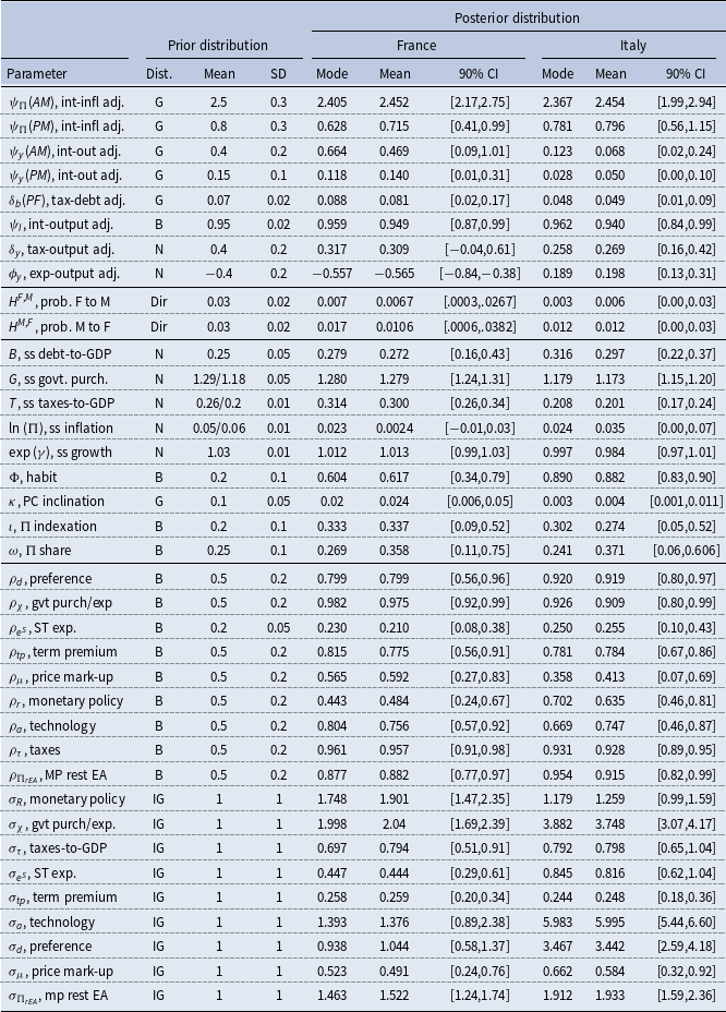


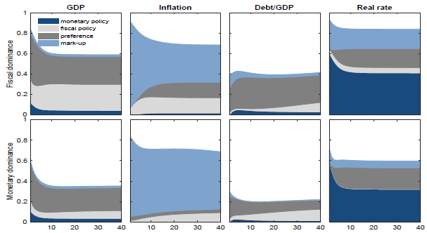
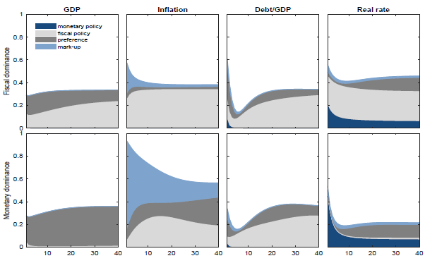
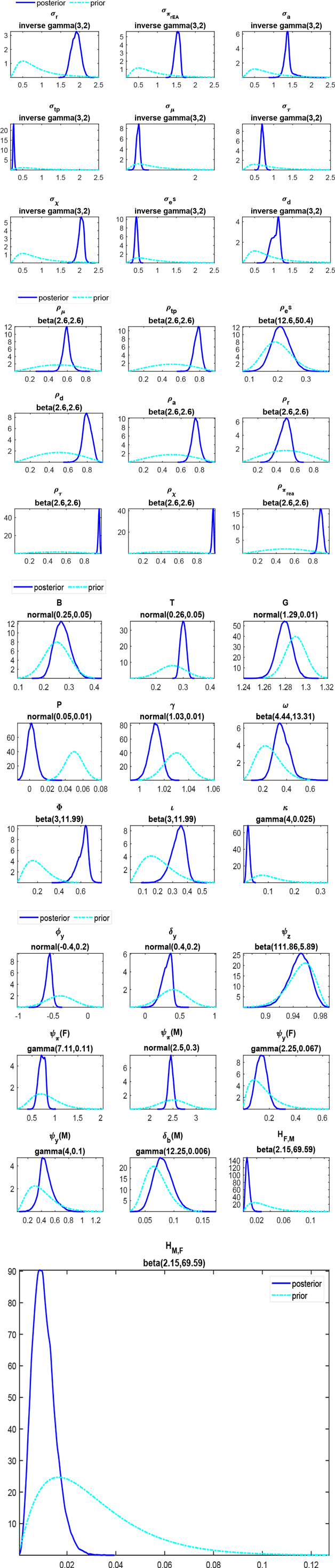
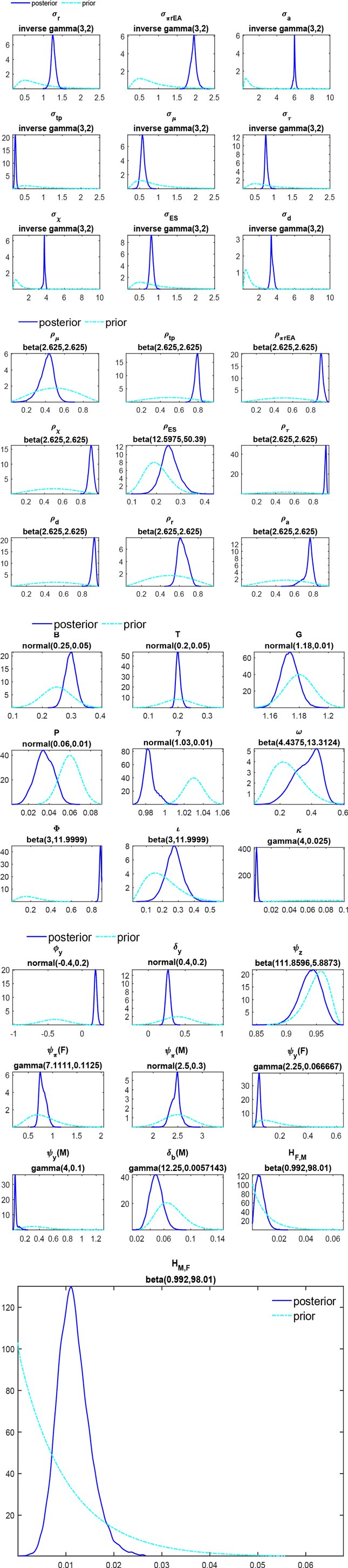
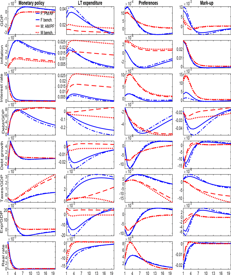


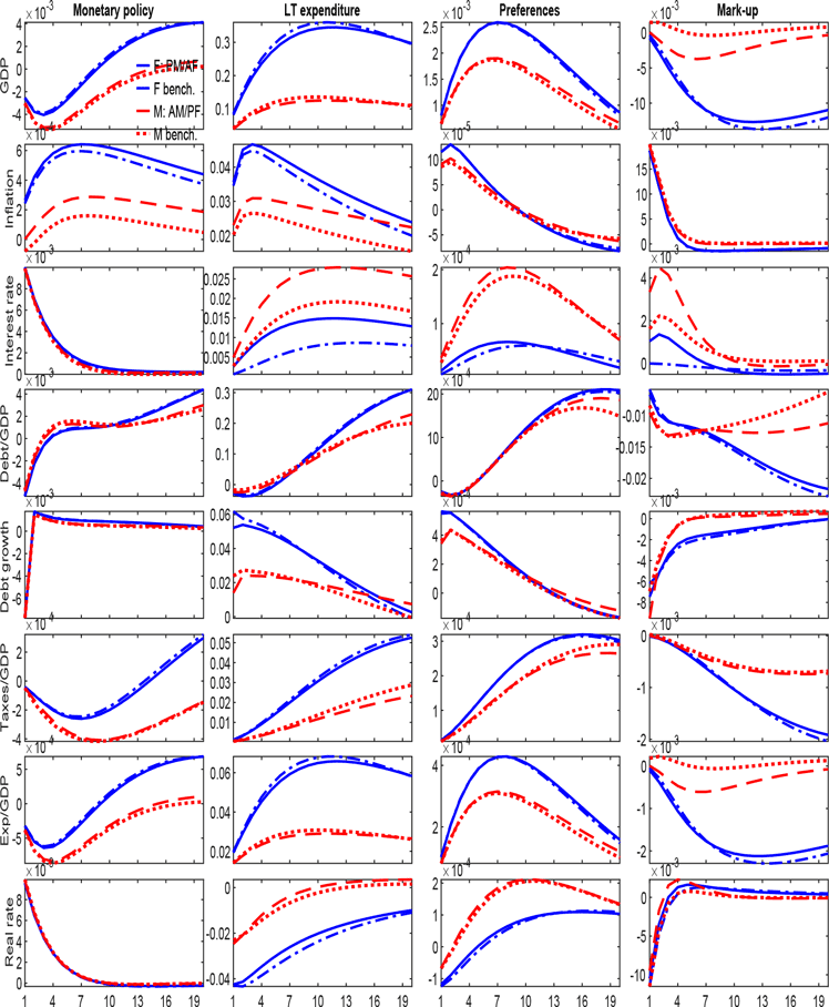


 Open access