


1. Introduction
Flow and transport simulations of fractured formations are relevant in many applications such as nuclear waste deposition (Hartley & Joyce Reference Hartley and Joyce2013; Joyce et al. Reference Joyce, Hartley, Applegate, Hoek and Jackson2014), CO $_2$
subsurface storage (Shao et al. Reference Shao, Matthäi, Driesner and Gross2021, Reference Shao, Boon, Youssef, Kurtev, Benson and Matthäi2022), enhanced geothermal systems (Olasolo et al. Reference Olasolo, Juárez, Morales, D’Amico and Liarte2016), groundwater management (Kitanidis Reference Kitanidis2015) and oil recovery processes (Srinivasan et al. Reference Srinivasan2021). With fractures often representing highly conductive flow conduits, they have a significant effect on flow and transport in natural porous media. Moreover, fractures can cover a wide range of scales starting at the grain level with microfractures (Anders, Laubach & Scholz Reference Anders, Laubach and Scholz2014). These fractures merge and form increasingly larger structures leading to a hierarchy that may span several orders of magnitude (Bonnet et al. Reference Bonnet, Bour, Odling, Davy, Main, Cowie and Berkowitz2001).
$_2$
subsurface storage (Shao et al. Reference Shao, Matthäi, Driesner and Gross2021, Reference Shao, Boon, Youssef, Kurtev, Benson and Matthäi2022), enhanced geothermal systems (Olasolo et al. Reference Olasolo, Juárez, Morales, D’Amico and Liarte2016), groundwater management (Kitanidis Reference Kitanidis2015) and oil recovery processes (Srinivasan et al. Reference Srinivasan2021). With fractures often representing highly conductive flow conduits, they have a significant effect on flow and transport in natural porous media. Moreover, fractures can cover a wide range of scales starting at the grain level with microfractures (Anders, Laubach & Scholz Reference Anders, Laubach and Scholz2014). These fractures merge and form increasingly larger structures leading to a hierarchy that may span several orders of magnitude (Bonnet et al. Reference Bonnet, Bour, Odling, Davy, Main, Cowie and Berkowitz2001).
Different approaches have been put forward to simulate flow and transport in fractured formations. On one hand, there are methods that resolve fractures with specialised fracture-conforming finite-element (Juanes, Samper & Molinero Reference Juanes, Samper and Molinero2002) or finite-volume grids (Ding, Basquet & Bourbiaux Reference Ding, Basquet and Bourbiaux2006; Karimi-Fard & Durlofsky Reference Karimi-Fard and Durlofsky2016) or combinations thereof (Matthäi et al. Reference Matthäi, Mezentsev and Belayneh2007). While some of these methods neglect matrix flow, which led to the discrete fracture network (DFN) method (Hyman et al. Reference Hyman, Karra, Makedonska, Gable, Painter and Viswanathan2015; Huang et al. Reference Huang, Liu, Jiang and Cheng2021), the discrete fracture matrix (DFM) method accounts for it; see e.g. (Viswanathan et al. Reference Viswanathan2022, figure 8). Depending on the level of resolution, DFM methods may resolve all fractures from a wide range of scales, or only large fractures while homogenising small ones and treating them as part of the matrix continuum. The resolved fractures are either presented as arrays of grid elements or reduced to lower-dimensional manifolds (Lei, Latham & Tsang Reference Lei, Latham and Tsang2017). To reduce the geometrical complexity of the finite element/volume grids, methods have been devised that embed fractures in Cartesian meshes (Lee, Lough & Jensen Reference Lee, Lough and Jensen2001). A popular example from this group of methods is the embedded discrete fracture model (EDFM) (Li & Lee Reference Li and Lee2008; Hajibeygi, Karvounis & Jenny Reference Hajibeygi, Karvounis and Jenny2011; Formaggia et al. Reference Formaggia, Fumagalli, Scotti and Ruffo2014; Moinfar et al. Reference Moinfar, Varavei, Sepehrnoori and Johns2014; Schwenck et al. Reference Schwenck, Flemisch, Helmig and Wohlmuth2015; Flemisch, Fumagalli & Scotti Reference Flemisch, Fumagalli and Scotti2016; Jiang & Younis Reference Jiang and Younis2017). While the EDFM adopts non-conforming meshes and reduces the complexity in this regard, it comes at the expense of a more complex fracture-matrix coupling formulation (Wong et al. Reference Wong, Doster, Geiger, Knut-Andreas and Møyner2021). However, since in DFN, DFM and EDFM simulations the fractures need to be explicitly resolved, the high accuracy of these methods comes at a price that becomes prohibitive for formations with wide fracture length distributions and/or high fracture densities (Berre, Doster & Keilegavlen Reference Berre, Doster and Keilegavlen2019, figure 4 or Joyce et al. Reference Joyce, Hartley, Applegate, Hoek and Jackson2014, p. 1240). Viswanathan et al. (Reference Viswanathan2022) state for example in their recent review: ‘… even the latest and cutting-edge DFN/DFM simulators can only resolve tens of thousands of fractures, not the millions present at field sites, although it can be argued that fracture locations will rarely be known at a field site at all relevant length scales’.
As an alternative to fracture-resolving methods, approaches have been devised that combine the flow transmissibility of fracture networks (and the matrix) into effective (tensor) permeabilities. These approaches are suitable for small, densely located (connected) fractures and are referred to as effective porous media (EPM) models. They rely on analytical (Oda Reference Oda1985) or numerical methods (e.g. Liu et al. Reference Liu, Li, Jiang and Huang2016; Romano et al. Reference Romano, Bigi, Carnevale, De’Haven Hyman, Karra, Valocchi, Tartarello and Battaglia2020) for the extraction of effective permeabilities. However, given the large range of length scales that fractures typically span, homogenisation volumes – also referred to as representative elementary volumes (REV) – may not exist for the definition of effective permeabilities: For example, Lee et al. (Reference Lee, Lough and Jensen2001, p. 1) write ‘…, in a naturally fractured formation, REVs can be too large to model with sufficient detail’. Despite these challenges, the EPM concept is widely used, since it allows for low-cost simulations of fractured formations, which has led to several EPM-based models: Firstly, DFM methods shall be mentioned that include a DFN description for large-scale fractures and couple it with an EPM representation for the matrix and unresolved fractures. Furthermore, there exist single continuum models, where matrix flow is typically neglected (e.g. Romano et al. Reference Romano, Bigi, Carnevale, De’Haven Hyman, Karra, Valocchi, Tartarello and Battaglia2020) and multi-continua models typically referred to as multi-rate mass transfer (MRMT) models (Haggerty & Gorelick Reference Haggerty and Gorelick1995; Harvey & Gorelick Reference Harvey and Gorelick1995). The latter are a generalisation of the dual porosity resp. mobile/immobile model. Despite the increasing level of refinement of these models, local effective parameters may generally not exist. For example, Berre et al. (Reference Berre, Doster and Keilegavlen2019) state in their recent review ‘…, there is generally no separation of length scales in fracture sizes; thus, upscaling into average properties often results in poor model quality’.
Given the limitations of existing methods, we focus in this work on formations with disconnected, highly conductive fractures that are of a size not much smaller than the scale of interest (Shapiro Reference Shapiro1987; Taylor, Pollard & Aydin Reference Taylor, Pollard and Aydin1999). Such fractures pose a particular challenge to existing approaches and were found in experiments to induce considerable secondary permeability (Su, Nimmo & Dragila Reference Su, Nimmo and Dragila2003). Since corresponding fractures typically appear in large numbers with their precise locations and characteristics being uncertain, we rely on a statistical description to determine the fractures. More specifically, our work is based on a non-local theory of porous media flow/transport that accounts for large-scale flow conduits, which first has been introduced at the pore scale (Delgoshaie et al. Reference Delgoshaie, Meyer, Jenny and Tchelepi2015; Jenny & Meyer Reference Jenny and Meyer2017; Meyer & Gomolinski Reference Meyer and Gomolinski2019). Later, that non-local methodology has been adapted by Jenny (Reference Jenny2020) for fractured formations leading to a new non-local dual media model. This model represents isolated fractures as contracted points with associated kernel functions that describe the expected flow exchange between fractures and matrix. The support of the kernel functions corresponds to the physical extent of the fractures. With the precise characteristics of the fractures being uncertain, the theory (Jenny Reference Jenny2020) does not provide the flow and pressure fields of fully resolved fractured formations but instead mean or expected flow and pressure fields that would result from an ensemble of formations sharing the same underlying fracture statistics. Further, it is assumed in Jenny (Reference Jenny2020) that the expected flow exchange between the fractures and the matrix is proportional to the expected pressure difference between the two domains with the magnitude of the kernel function providing the proportionality factor. The latter can be understood as a transfer coefficient that depends on the fracture statistics and the permeability of the porous matrix.
In the previous work, this transfer coefficient has been determined empirically by running Monte Carlo simulations (MCS) on an infinitely large domain with homogeneous fracture statistics. More specifically, a finite-size domain with periodic boundary conditions was used as an analogue to an infinite domain and the transfer coefficient could be extracted from the mean flow rate in the fractures. In this work, we aim to expand the model to account for statistical fracture distributions that are a function of space. Thus fractures are no longer homogeneously but instead heterogeneously distributed. Specifically, we present statistically one-dimensional cases, where the fractures are modelled as parallel plates with a spatially non-uniform distribution. For such fracture statistics, it is not possible to determine the transfer coefficient in the same way as periodic boundary conditions do not allow for arbitrary fracture statistics. Through numerical experiments using MCS, it was found, however, that the transfer coefficient at a location in the domain depends primarily on the statistics of fractures that have their centre points at that same location. Therefore, one can determine the transfer coefficient at an arbitrary point by running MCS on a periodic domain with homogeneous statistics being identical to the fractures at the point in question. In order to determine the transfer coefficient in the entire heterogeneous domain, MCS need to be repeated for all statistical states arising in the domain. This becomes prohibitive if the variation of these parameters is continuous. To alleviate this problem, a scaling law for the transfer coefficient will be presented, which allows us to determine transfer coefficients by running just two MCS and a single fracture simulation in total. With the resulting scaling law, spatially varying fracture statistics can be accounted for in the kernel-based model.
The rest of this work is divided into the following sections: § 2 first introduces the set-up of the MCS used for generating reference data. In particular, § 2.1 provides a detailed explanation of the implementation of the reference MCS, included for the sake of completeness (readers focusing on our new model generalisations may skip this subsection). Then the kernel-based model proposed by Jenny (Reference Jenny2020) is restated and the extension to heterogeneous fracture statistics is discussed. In § 2.3 the scaling law for the transfer coefficient is derived. In § 3.1 we compare the transfer coefficients calculated from the scaling law with those obtained from MCS data. In §§ 3.2 and 3.3 the proposed scaling law is applied for test cases where the fracture statistics vary discontinuously and continuously, and we compare the results from the model with the reference MCS data.
2. Method
We consider incompressible single-phase flow through a porous medium with embedded, isolated and highly conductive fractures. The flow is driven by a pressure gradient and the flow governing equation reads
 \begin{align} \frac {\partial \phi }{\partial t} - \frac {\partial }{\partial x_i}\left ( \frac {k_{ij}}{\mu } \frac {\partial p}{\partial x_j} \right ) = 0, \end{align}
where $\phi$
is the porosity of the fractured porous medium,
$\phi$
is the porosity of the fractured porous medium, $k_{ij}$
is the permeability tensor,
$k_{ij}$
is the permeability tensor, $\mu$
is the viscosity of the fluid and
$\mu$
is the viscosity of the fluid and $p$
is the pressure. Einstein summation notation is employed, wherein repeated indices are implicitly summed over the three spatial dimensions. We assume that the porosity is stationary and the viscosity constant, which leads to
$p$
is the pressure. Einstein summation notation is employed, wherein repeated indices are implicitly summed over the three spatial dimensions. We assume that the porosity is stationary and the viscosity constant, which leads to
 \begin{align} \frac {\partial }{\partial x_i}\left ( k_{ij} \frac {\partial p}{\partial x_j} \right ) = 0, \end{align}
or in normalised form to
 \begin{align} \frac {\partial }{\partial \hat {x}_i}\left ( \hat {k}_{ij} \frac {\partial \hat {p}}{\partial \hat {x}_j} \right ) = 0 \end{align}
and
 \begin{align} \hat {u}_i = -\hat {k}_{ij}\frac {\partial \hat {p}}{\partial \hat {x}_j} \end{align}
with
 \begin{align} \hat {x} = \frac {x}{l_{\textit{ref}}}, \hat {k}_{ij} = \frac {k_{ij}}{l_{\textit{ref}}^2}, \hat {u}_i = \frac {u_i}{u_{\textit{ref}}} \text{ and } \hat {p} = \frac {p}{\mu u_{\textit{ref}}}, \end{align}
where $l_{\textit{ref}}$
is the reference length,
$l_{\textit{ref}}$
is the reference length, $\rho _{\textit{ref}}$
the reference density of the fluid and
$\rho _{\textit{ref}}$
the reference density of the fluid and $u_{\textit{ref}}$
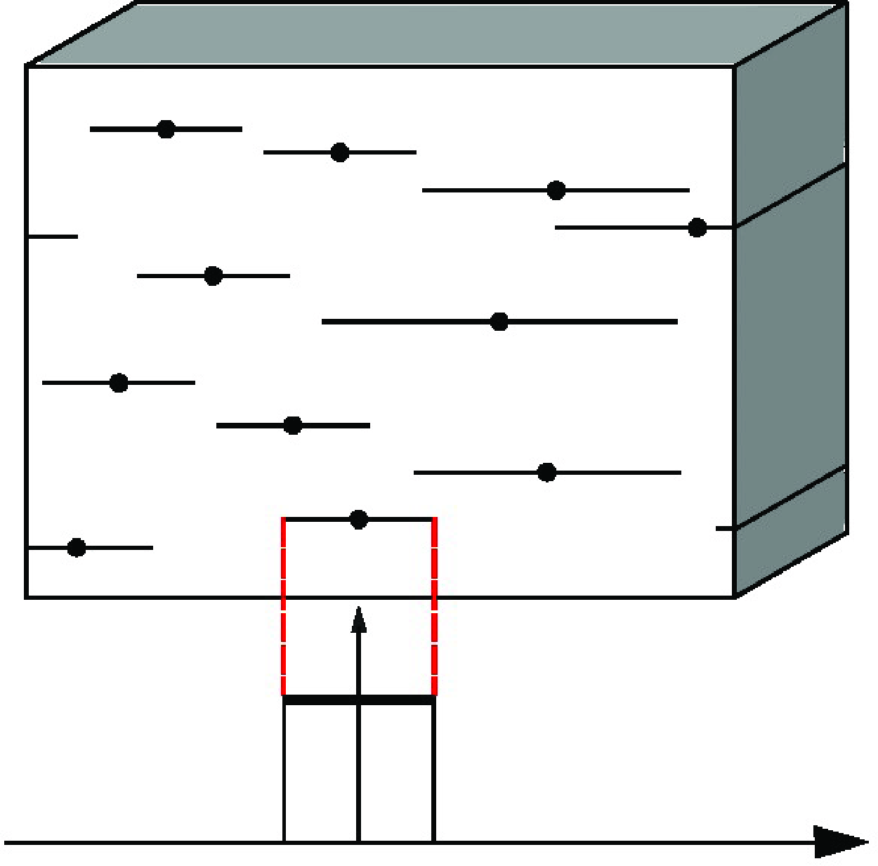
the reference velocity. From now on we focus on non-dimensional quantities and therefore, for the sake of simplicity, the hat symbol in (2.3) is omitted. In this work we focus on statistically one-dimensional scenarios, where all fractures have the same orientation. As shown in figure 1, a Cartesian coordinate system is considered with its
$u_{\textit{ref}}$
the reference velocity. From now on we focus on non-dimensional quantities and therefore, for the sake of simplicity, the hat symbol in (2.3) is omitted. In this work we focus on statistically one-dimensional scenarios, where all fractures have the same orientation. As shown in figure 1, a Cartesian coordinate system is considered with its $x$
-coordinate aligned with the fracture orientation. A mean pressure gradient in the
$x$
-coordinate aligned with the fracture orientation. A mean pressure gradient in the $x$
-direction is imposed, and the fracture statistics vary only along the
$x$
-direction is imposed, and the fracture statistics vary only along the $x$
-coordinate. In the
$x$
-coordinate. In the $y$
-direction, periodic boundary conditions are imposed, and spatial homogeneity in
$y$
-direction, periodic boundary conditions are imposed, and spatial homogeneity in $z$
-direction is considered (no pressure change or flow in
$z$
-direction is considered (no pressure change or flow in $z$
-direction).
$z$
-direction).
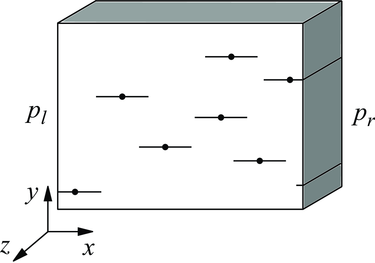
Figure 1. Porous medium with embedded, isolated, parallel fractures. The fractures are abstracted as line segments, where the black dots mark the fracture centres. The $x$
-direction of the Cartesian coordinate system is aligned with the fracture orientation. A mean pressure gradient is imposed in the
$x$
-direction of the Cartesian coordinate system is aligned with the fracture orientation. A mean pressure gradient is imposed in the $x$
-direction, and the fracture statistics may vary along the
$x$
-direction, and the fracture statistics may vary along the $x$
-coordinate. The pressure imposed on the left and right boundary is denoted as
$x$
-coordinate. The pressure imposed on the left and right boundary is denoted as $p_l$
and
$p_l$
and $p_r$
respectively. In the
$p_r$
respectively. In the $y$
-direction, periodic boundary conditions are imposed.
$y$
-direction, periodic boundary conditions are imposed.
2.1. Monte Carlo simulation
In the MCS we consider a finite domain $\Omega =[0,L_x]\times [0,L_y]$
of length
$\Omega =[0,L_x]\times [0,L_y]$
of length $L_x$
and height
$L_x$
and height $L_y$
with periodic boundary conditions in the
$L_y$
with periodic boundary conditions in the $y$
-direction. A mean pressure gradient is imposed in the
$y$
-direction. A mean pressure gradient is imposed in the $x$
-direction. The fracture centres are randomly placed within the sampling region
$x$
-direction. The fracture centres are randomly placed within the sampling region $\Omega ^{sampling}=[-{l_{f, max}}/{2}, L_x + {l_{f, max}}/{2}]\times [0, L_y]$
, which extends
$\Omega ^{sampling}=[-{l_{f, max}}/{2}, L_x + {l_{f, max}}/{2}]\times [0, L_y]$
, which extends $\Omega$
at the left and right boundaries by half the length of the longest possible fracture
$\Omega$
at the left and right boundaries by half the length of the longest possible fracture $l_{f, max}$
. This extended sampling domain is required to account for fractures with centres lying outside of the domain but intersecting with the domain boundaries. With the set-up being statistically homogeneous inthe
$l_{f, max}$
. This extended sampling domain is required to account for fractures with centres lying outside of the domain but intersecting with the domain boundaries. With the set-up being statistically homogeneous inthe $y$
-direction, the sampling region in the
$y$
-direction, the sampling region in the $x$
-direction was divided into thin slices
$x$
-direction was divided into thin slices ${\rm d}\Omega (x)$
being parallel to the
${\rm d}\Omega (x)$
being parallel to the $y$
–
$y$
– $z$
plane. With the fracture centres being uniformly distributed in the sampling region, the number of fractures
$z$
plane. With the fracture centres being uniformly distributed in the sampling region, the number of fractures $N_f(x)$
lying within a slice
$N_f(x)$
lying within a slice ${\rm d}\Omega (x)$
follows a binomial distribution with the probability mass function
${\rm d}\Omega (x)$
follows a binomial distribution with the probability mass function
 \begin{align} f(N_f) = \binom {\frac {1}{p} \rho _f |{\rm d}\Omega |}{N_f}p^{N_f}(1-p)^{\frac {1}{p} \rho _f |{\rm d}\Omega |-N_f}, \end{align}
where $p$
is the probability that a randomly sampled fracture lies inside
$p$
is the probability that a randomly sampled fracture lies inside ${\rm d}\Omega (x)$
in a Bernoulli experiment, which is a freely chosen parameter and should approach zero. In all the MCS,
${\rm d}\Omega (x)$
in a Bernoulli experiment, which is a freely chosen parameter and should approach zero. In all the MCS, $p$
was chose to be
$p$
was chose to be $0.1$
and the slice thickness was set to
$0.1$
and the slice thickness was set to $|{\rm d}\Omega (x)|=0.001L_x$
. Note that the expected number of fractures given by (2.6) is
$|{\rm d}\Omega (x)|=0.001L_x$
. Note that the expected number of fractures given by (2.6) is $\mathbb{E}(N_f) = \rho _f(x) |{\rm d}\Omega (x)|$
and the variance is
$\mathbb{E}(N_f) = \rho _f(x) |{\rm d}\Omega (x)|$
and the variance is $\mathbb{V}(N_f) = \rho _f(x) |{\rm d}\Omega (x)|(1-p)$
. Placing fractures in this way, rather than distributing
$\mathbb{V}(N_f) = \rho _f(x) |{\rm d}\Omega (x)|(1-p)$
. Placing fractures in this way, rather than distributing $\rho _f(x) |{\rm d}\Omega (x)|$
fractures within
$\rho _f(x) |{\rm d}\Omega (x)|$
fractures within ${\rm d}\Omega (x)$
, is important in order to account for the fact that the fracture number density
${\rm d}\Omega (x)$
, is important in order to account for the fact that the fracture number density $\rho _f(x)$
is the expected number of fractures per unit volume, while the actual number varies between single realisations. For each slice
$\rho _f(x)$
is the expected number of fractures per unit volume, while the actual number varies between single realisations. For each slice ${\rm d}\Omega (x)$
, we sample the number of fractures
${\rm d}\Omega (x)$
, we sample the number of fractures $N_f(x)$
according to (2.6). The resulting
$N_f(x)$
according to (2.6). The resulting $N_f(x)$
fractures are distributed randomly and uniformly within
$N_f(x)$
fractures are distributed randomly and uniformly within ${\rm d}\Omega (x)$
with the extra constraint that they do not intersect with each other.
${\rm d}\Omega (x)$
with the extra constraint that they do not intersect with each other.
For the numerical flow computations, i.e. to solve (2.3), a classical cell-centred finite volume method with a uniform Cartesian $n_x \times n_y$
grid was used. The grid has the same spacing in
$n_x \times n_y$
grid was used. The grid has the same spacing in $x$
- and
$x$
- and $y$
-directions, i.e.
$y$
-directions, i.e. $h = {L_x}/{n_x} = {L_y}/{n_y}$
. The upscaled permeability tensor in a cell is
$h = {L_x}/{n_x} = {L_y}/{n_y}$
. The upscaled permeability tensor in a cell is
 \begin{align} {\boldsymbol k} = \begin{bmatrix} k_x & 0 \\ 0 & k_y \end{bmatrix}, \end{align}
where
 \begin{align} k_{x} & = \frac {k_f a_f + k_m (h-a_f)}{h} \\[6pt] \nonumber \end{align}
and
 \begin{align} k_{y} & = \frac {h}{\dfrac {a_f}{k_f}+\dfrac {h-a_f}{k_m}}, \\[6pt] \nonumber \end{align}
if the cell is intersected by a fracture with aperture $a_f$
, and
$a_f$
, and
 \begin{align} k_{x} \, =\, k_{y} & =\, k_m \end{align}
otherwise; see (Renard & De Marsily Reference Renard and De Marsily1997) and (Kasap & Lake Reference Kasap and Lake1990). Note that $k_f$
and
$k_f$
and $k_m$
represent the fracture and matrix permeabilities, respectively, and are constants such that
$k_m$
represent the fracture and matrix permeabilities, respectively, and are constants such that ${k_f}/k_m\gg 1$
(Phillips Reference Phillips1991). Further, we assume that
${k_f}/k_m\gg 1$
(Phillips Reference Phillips1991). Further, we assume that $a_f$
does not vary along a fracture and is not larger than the grid spacing
$a_f$
does not vary along a fracture and is not larger than the grid spacing $h$
. To determine the numerical fluxes at cell interfaces, harmonically averaged permeability values are employed, and a direct solver is employed to solve the resulting linear system. Figure 2 shows realisations of two pressure fields with space-stationary fracture statistics. The solution of each realisation gets partitioned into the matrix and fracture pressure fields
$h$
. To determine the numerical fluxes at cell interfaces, harmonically averaged permeability values are employed, and a direct solver is employed to solve the resulting linear system. Figure 2 shows realisations of two pressure fields with space-stationary fracture statistics. The solution of each realisation gets partitioned into the matrix and fracture pressure fields
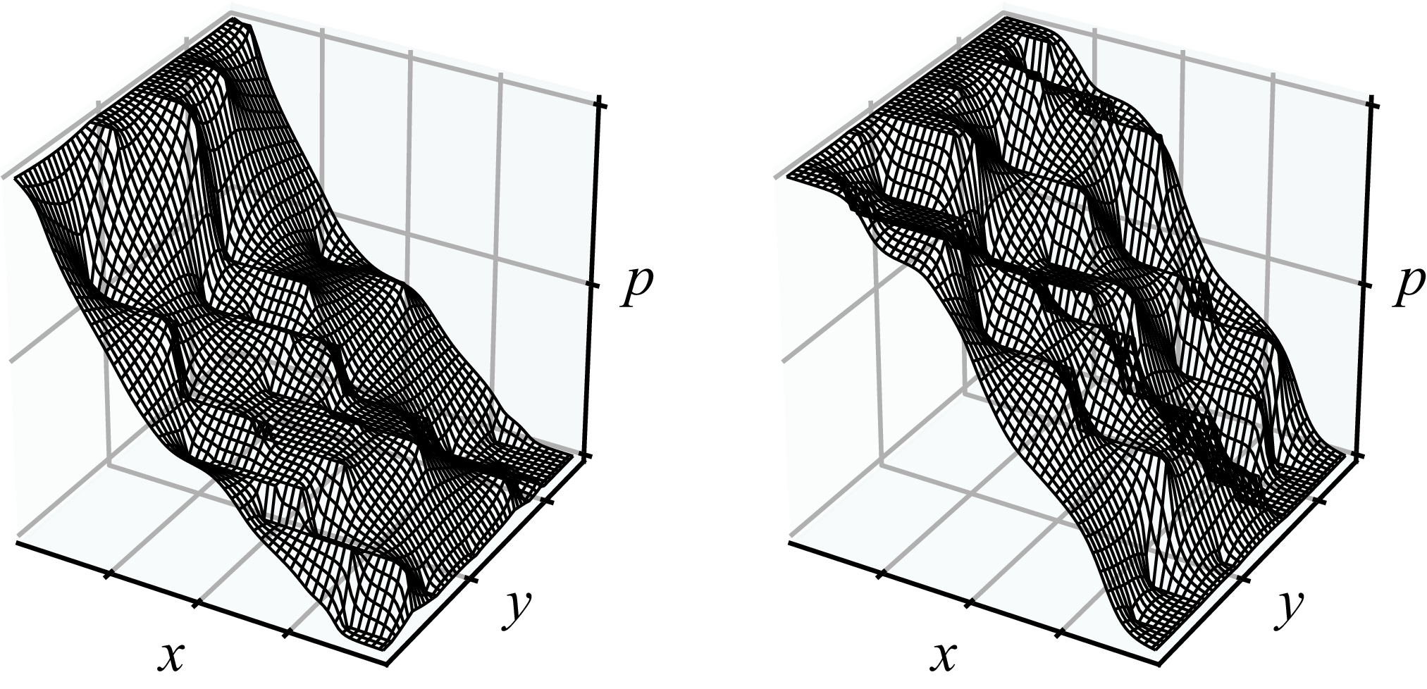
Figure 2. Realisations of two pressure fields with space-stationary fracture statistics.
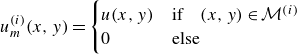
 \begin{align} p^{(i)}_m(x, y) & = \begin{cases} p(x, y) & \text{if} \quad (x, y) \in \mathcal{M}^{(i)} \\ 0 & \text{else} \end{cases} \end{align}
and
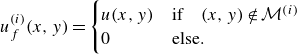
 \begin{align} p^{(i)}_f(x, y) & = \begin{cases} \frac {1}{|V_f(x, y)|}\int _{V_f(x, y)} p(x, y) {\rm d}V_f(x, y) & \text{if} \quad (x, y) \in \mathcal{F}^{(i)} \\ 0 & \text{else,} \end{cases} \end{align}
respectively, and correspondingly into the matrix and fracture flow fields
 \begin{align} u^{(i)}_m(x, y) & = \begin{cases} u(x, y) & \text{if} \quad (x, y) \in \mathcal{M}^{(i)} \\ 0 & \text{else} \end{cases} \end{align}
and
 \begin{align} u^{(i)}_f(x, y) & = \begin{cases} u(x, y) & \text{if} \quad (x, y) \notin \mathcal{M}^{(i)} \\ 0 & \text{else.} \end{cases} \end{align}
Here $\mathcal{M}^{(i)}$
and
$\mathcal{M}^{(i)}$
and $\mathcal{F}^{(i)}$
are the sets of matrix points and fracture centres of the
$\mathcal{F}^{(i)}$
are the sets of matrix points and fracture centres of the $i$
th realisation, and
$i$
th realisation, and $V_f(x, y)$
denotes the volume of the fracture with its centre at
$V_f(x, y)$
denotes the volume of the fracture with its centre at $(x, y)$
. The partitioned fields are averaged to obtain the mean fields (expectations)
$(x, y)$
. The partitioned fields are averaged to obtain the mean fields (expectations)
 \begin{align} \bar {p}_m(x) & = \bar {p}_m(x, y) = \lim \limits _{n \to \infty }\frac {\sum _{i=1}^{n}{\mathbb{I}}_{\mathcal{M}^{(i)}}\left (x, y\right )p_m^{(i)}(x, y)}{\sum _{i=1}^{n}{\mathbb{I}}_{\mathcal{M}^{(i)}}\left (x, y\right )}, \\[-12pt] \nonumber \end{align}
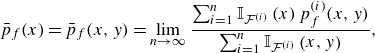 \begin{align} \bar {p}_f(x) & = \bar {p}_f(x, y) = \lim \limits _{n \to \infty }\frac {\sum _{i=1}^{n}{\mathbb{I}}_{\mathcal{F}^{(i)}}\left (x\right )p_f^{(i)}(x, y)}{\sum _{i=1}^{n}{\mathbb{I}}_{\mathcal{F}^{(i)}}\left (x, y\right )}, \\[-12pt] \nonumber \end{align}
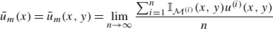 \begin{align} \bar {u}_m(x) & = \bar {u}_m(x, y) = \lim \limits _{n \to \infty } \frac {\sum _{i=1}^{n}{\mathbb{I}}_{\mathcal{M}^{(i)}}(x, y)u^{(i)}(x, y)}{n} \\[-12pt] \nonumber \end{align}
 \begin{align} \bar {u}_f(x) & = \bar {u}_f(x, y) = \lim \limits _{n \to \infty } \frac {\sum _{i=1}^{n}\left (1-{\mathbb{I}}_{\mathcal{M}^{(i)}}(x, y)\right )u^{(i)}(x, y)}{n} \\[6pt] \nonumber \end{align}
on the respective domains. Note that
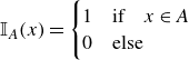 \begin{align} \mathbb{I}_A(x) = \begin{cases} 1 & \text{if} \quad x \in A \\ 0 & \text{else} \end{cases} \end{align}
is an indicator function. In the numerical implementation the matrix and fracture pressures in cell $(I, J)$
of realisation
$(I, J)$
of realisation $(i)$
are set to
$(i)$
are set to
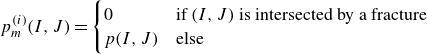 \begin{align} p^{(i)}_m(I, J) & = \begin{cases} 0 & \text{if $(I, J)$ is intersected by a fracture} \\ p(I, J) & \text{else} \end{cases} \end{align}
and
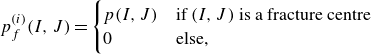 \begin{align} p^{(i)}_f(I, J) & = \begin{cases} p(I, J) & \text{if $(I, J)$ is a fracture centre} \\ 0 & \text{else,} \end{cases} \end{align}
respectively. Note that it is assumed that the average pressure inside a fracture is approximately equal to the pressure at its centre, which is reasonable for highly conductive fractures (as seen for example in figure 2).
2.2. Kernel-based model
Because of the domain set-up introduced previously, the expected fracture and matrix pressures, $\bar {p}_f(x)$
and
$\bar {p}_f(x)$
and $\bar {p}_m(x)$
, respectively, are functions of the
$\bar {p}_m(x)$
, respectively, are functions of the $x$
-coordinate only. Note that by definition
$x$
-coordinate only. Note that by definition $\bar {p}_f(x)$
refers to the mean pressure of all fractures with their centres at
$\bar {p}_f(x)$
refers to the mean pressure of all fractures with their centres at $x$
from an infinitely large ensemble. We follow the approach by Jenny (Reference Jenny2020, p. 4), that is, the expected flow exchange between fractures with centres at
$x$
from an infinitely large ensemble. We follow the approach by Jenny (Reference Jenny2020, p. 4), that is, the expected flow exchange between fractures with centres at $x'$
and the location
$x'$
and the location $x$
in the matrix domain is assumed to be proportional to
$x$
in the matrix domain is assumed to be proportional to $\bar {p}_f(x')-\bar {p}_m(x)$
. As outlined in Jenny (Reference Jenny2020), for a domain
$\bar {p}_f(x')-\bar {p}_m(x)$
. As outlined in Jenny (Reference Jenny2020), for a domain $\Omega = [0, L_x]$
this leads to the mass balance
$\Omega = [0, L_x]$
this leads to the mass balance
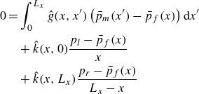 \begin{align} 0= & \int _0^{L_x} \hat {g}(x, x') \left ( \bar {p}_m(x') - \bar {p}_f(x)\right ) {\rm d}x' \nonumber \\ & + \hat {k}(x,0) \frac {p_l-\bar {p}_f(x)}{x} \nonumber \\ & + \hat {k}(x,L_x) \frac {p_r-\bar {p}_f(x)}{L_x-x} \end{align}
in the fracture domain at location $x$
and to the balance
$x$
and to the balance
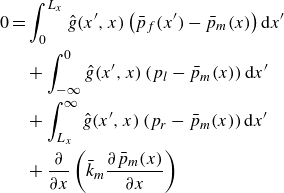 \begin{align} 0= & \int _0^{L_x} \hat {g}(x', x) \left ( \bar {p}_f(x') - \bar {p}_m(x)\right ) {\rm d}x' \nonumber \\ & + \int _{-\infty }^{0}\hat {g}(x', x) \left (p_l - \bar {p}_m(x)\right ) {\rm d}x' \nonumber \\ & + \int _{L_x}^{\infty }\hat {g}(x', x) \left (p_r - \bar {p}_m(x)\right ) {\rm d}x' \nonumber \\ & + \frac {\partial }{\partial x} \left ( \bar {k}_m \frac {\partial \bar {p}_m(x)}{\partial x} \right ) \end{align}
at point $x$
in the matrix domain. Note that these are coupled integro-differential equations employing the kernel functions
$x$
in the matrix domain. Note that these are coupled integro-differential equations employing the kernel functions $\hat {g}(x, x')$
and
$\hat {g}(x, x')$
and $\hat {k}(x, x')$
, where the shape of the kernel depends on the geometry of the fractures. In this work, like in Jenny (Reference Jenny2020, p. 11), we adopt kernels with the top-hat shape, that is,
$\hat {k}(x, x')$
, where the shape of the kernel depends on the geometry of the fractures. In this work, like in Jenny (Reference Jenny2020, p. 11), we adopt kernels with the top-hat shape, that is,
 \begin{align} &\hat {g}(x, x') =\begin{cases} \bar {g} & \quad \text{if} \quad \left |x-x'\right |\lt \frac {l_f}{2} \\ 0 & \quad \text{else} \\ \end{cases} \\[6pt] \nonumber \end{align}
and
 \begin{align} &\hat {k}(x, x') =\begin{cases} \bar {k} & \quad \text{if} \quad \left |x-x'\right |\lt \frac {l_f}{2} \\ 0 & \quad \text{else,} \\ \end{cases} \\[6pt] \nonumber \end{align}
where $l_f$
is the fracture length. Flow exchange between fracture and matrix domains is described by the first right-hand-side terms in (2.22) and (2.23); as argued, they are linear in the pressure difference
$l_f$
is the fracture length. Flow exchange between fracture and matrix domains is described by the first right-hand-side terms in (2.22) and (2.23); as argued, they are linear in the pressure difference $\bar {p}_f(x')-\bar {p}_m(x)$
. The second and third right-hand-side terms in (2.22) account for direct connections of fractures centred at
$\bar {p}_f(x')-\bar {p}_m(x)$
. The second and third right-hand-side terms in (2.22) account for direct connections of fractures centred at $x$
with the left and right boundaries, respectively; note that
$x$
with the left and right boundaries, respectively; note that $p_l$
and
$p_l$
and $p_r$
denote the corresponding boundary pressure values. Similarly, the second and third right-hand-side terms in (2.23) account for boundary effects in the mean matrix mass balance. More precisely, they consider the exchange between the matrix domain and fractures with centres outside of the domain; note their similarity with the first term in (2.23). Finally, the last right-hand-side term in (2.23), with the effective mean matrix permeability
$p_r$
denote the corresponding boundary pressure values. Similarly, the second and third right-hand-side terms in (2.23) account for boundary effects in the mean matrix mass balance. More precisely, they consider the exchange between the matrix domain and fractures with centres outside of the domain; note their similarity with the first term in (2.23). Finally, the last right-hand-side term in (2.23), with the effective mean matrix permeability $\bar {k}_m$
, accounts for Darcy-type flow exchange between a point in the matrix domain with its immediate neighbourhood.
$\bar {k}_m$
, accounts for Darcy-type flow exchange between a point in the matrix domain with its immediate neighbourhood.
For statistically homogeneous cases, as in Jenny (Reference Jenny2020, p. 13), the effective mean matrix permeability $\bar k_m$
and the kernel amplitudes
$\bar k_m$
and the kernel amplitudes $\bar k$
and
$\bar k$
and $\bar g$
are obtained as
$\bar g$
are obtained as
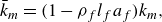 \begin{align} \bar {k}_m & = (1-\rho _fl_fa_f)k_m, \\[-10pt] \nonumber \end{align}
 \begin{align} \bar {k} & = \rho _fa_fk_f, \\[-10pt] \nonumber \end{align}
 \begin{align} \bar {g} & = \frac {12\ |\bar {u}_f^\infty |}{l_f^3|\nabla _x^\infty p|}, \\[6pt] \nonumber \end{align}
respectively, where $\nabla _x^\infty p$
and
$\nabla _x^\infty p$
and $\bar {u}_f^\infty$
denote mean pressure gradient and mean flow rate through the fracture in an infinitely large domain with isolated fractures of the same length. The scalar
$\bar {u}_f^\infty$
denote mean pressure gradient and mean flow rate through the fracture in an infinitely large domain with isolated fractures of the same length. The scalar $\bar {g}$
relates the expected flow exchange between the fractures and the porous matrix to the expected pressure difference between the two domains and can be understood as a transfer coefficient. It is worth pointing out that the only empirical value required for model closure is the normalised mean volumetric flow rate
$\bar {g}$
relates the expected flow exchange between the fractures and the porous matrix to the expected pressure difference between the two domains and can be understood as a transfer coefficient. It is worth pointing out that the only empirical value required for model closure is the normalised mean volumetric flow rate ${(|\bar {u}_f^\infty |)}/{(|\nabla _x^\infty p|)}$
through the fractures in an infinitely long domain subjected to a mean pressure gradient. In practice we resorted to a long periodic domain with an imposed pressure gradient in the
${(|\bar {u}_f^\infty |)}/{(|\nabla _x^\infty p|)}$
through the fractures in an infinitely long domain subjected to a mean pressure gradient. In practice we resorted to a long periodic domain with an imposed pressure gradient in the $x$
-direction. More details about the model for homogeneous fracture statistics and about the numerical solution algorithm can be found in Jenny (Reference Jenny2020).
$x$
-direction. More details about the model for homogeneous fracture statistics and about the numerical solution algorithm can be found in Jenny (Reference Jenny2020).
For spatially variable fracture statistics – being the focus of the present paper – the average volume occupied by the matrix domain (quantified by the first factor in (2.26)) varies, and thus (2.26) needs to be generalised as
 \begin{align} &\bar {k}_m (x) = \left (1-\int _{-\infty }^{\infty }\rho _f(x) a_f(x) \mathbb{I}_f(x, x') {\rm d}x'\right )k_m, \\[6pt] \nonumber \end{align}
with
 \begin{align} & \mathbb{I}_f(x, x') = \begin{cases} 1 & \quad \text{if} \quad \left |x-x'\right |\lt \frac {l_f(x)}{2} \\ 0 & \quad \text{else.} \end{cases} \\[6pt] \nonumber \end{align}
The integral term represents the effective fracture volume fraction at point $x$
. However, as fractures are assumed to occupy only a small volume fraction, we typically have
$x$
. However, as fractures are assumed to occupy only a small volume fraction, we typically have $\bar {k}_m \approx k_m$
. The kernel amplitude
$\bar {k}_m \approx k_m$
. The kernel amplitude $\bar {k}(x)$
can be calculated in the same way as in (2.27). Instead of taking a constant value, it varies as the fracture statistics vary. The transfer coefficient
$\bar {k}(x)$
can be calculated in the same way as in (2.27). Instead of taking a constant value, it varies as the fracture statistics vary. The transfer coefficient $\bar {g}(x)$
can no longer be determined in the same way as in the statistically homogeneous case, since a periodically repeating domain may not be compatible with arbitrarily varying statistics. It was found, however, that at any given point
$\bar {g}(x)$
can no longer be determined in the same way as in the statistically homogeneous case, since a periodically repeating domain may not be compatible with arbitrarily varying statistics. It was found, however, that at any given point $x$
,
$x$
, $\bar {g}(x)$
depends primarily on the parameters of the fractures with centres at
$\bar {g}(x)$
depends primarily on the parameters of the fractures with centres at $x$
(for evidence, please refer to § 3). One can therefore determine the transfer coefficient
$x$
(for evidence, please refer to § 3). One can therefore determine the transfer coefficient $g(x)$
for every point
$g(x)$
for every point $x$
according to (2.28), which implies running MCS with long, statistically homogeneous domains and the same fracture statistics as at point
$x$
according to (2.28), which implies running MCS with long, statistically homogeneous domains and the same fracture statistics as at point $x$
.
$x$
.
2.3. Scaling law for the transfer coefficient
In order to avoid the need of many expensive MCS studies to determine the kernel parameters for a potentially wide range of fracture statistics in the heterogeneous domains, analytical relations respectively scaling laws shall be derived next. From dimension analysis, it can be shown that
 \begin{align} \left [\bar {g}\right ] & = \left [L^{-1}\right ]. \end{align}
here, L denotes the dimension of length. According to the Buckingham theorem, the dependency of $\bar {g}$
on the parameters
$\bar {g}$
on the parameters $ ( \rho _f, l_f, a_f, k_f, k_m )$
can be reduced to the dependency of the following dimensionless variables
$ ( \rho _f, l_f, a_f, k_f, k_m )$
can be reduced to the dependency of the following dimensionless variables
 \begin{align} \bar {g}l_f \sim \left (\rho _f l_f^2\right )^{\alpha }\left (\frac {k_m}{l_f^2}\right )^{\beta } \left (\frac {l_f}{a_f}\right )^{\gamma } \left ( \frac {k_f}{k_m} \right )^\delta. \end{align} $\alpha$
,
$\alpha$
, $\beta$
,
$\beta$
, $\gamma$
and
$\gamma$
and $\delta$
are real-valued exponents determining the influence of each dimensionless group. As we assume that
$\delta$
are real-valued exponents determining the influence of each dimensionless group. As we assume that $k_f \gg k_m$
and
$k_f \gg k_m$
and $l_f \gg a_f$
, the fracture permeability and the aperture do not influence the flow exchange significantly. Thus we keep
$l_f \gg a_f$
, the fracture permeability and the aperture do not influence the flow exchange significantly. Thus we keep $\frac {k_f}{k_m}$
and
$\frac {k_f}{k_m}$
and $\frac {a_f}{l_f}$
fixed here, and (2.32) reduces to
$\frac {a_f}{l_f}$
fixed here, and (2.32) reduces to
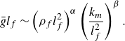 \begin{align} \bar {g}l_f \sim \left (\rho _f l_f^2\right )^{\alpha }\left (\frac {k_m}{l_f^2}\right )^{\beta }. \end{align}

Figure 3. Pressure fields around fractures with (a) small and (b) large relative distance between each other. Fractures are indicated as red lines. Panel (c) shows transverse pressure profiles (blue line, case with high fracture number density; orange, case with low fracture number density).
According to (2.28), $\bar {g}$
depends linearly on the mean flow rate
$\bar {g}$
depends linearly on the mean flow rate $\bar {u}_f^\infty$
through the fractures, and due to the linearity of the governing equation (2.3),
$\bar {u}_f^\infty$
through the fractures, and due to the linearity of the governing equation (2.3), $\bar {u}_f^\infty$
depends linearly on the permeability, from which follows that
$\bar {u}_f^\infty$
depends linearly on the permeability, from which follows that $\beta = 1$
and
$\beta = 1$
and
 \begin{align} \bar {g}l_f \sim \left (\rho _f l_f^2\right )^{\alpha }\left (\frac {k_m}{l_f^2}\right ). \end{align}
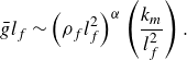
Rearranging (2.34) leads to
 \begin{align} \frac {\bar {g}l_f^3}{k_m} \sim \left (\rho _f l_f^2\right )^{\alpha } \end{align}
with $\alpha$
being the only scaling parameter. Note that the dimensionless geometrical parameter
$\alpha$
being the only scaling parameter. Note that the dimensionless geometrical parameter $\rho _f l_f^2$
describes the average spacing between fractures in relation to their length, and to determine
$\rho _f l_f^2$
describes the average spacing between fractures in relation to their length, and to determine $\alpha$
, we consider the following thought experiment. For very small values of
$\alpha$
, we consider the following thought experiment. For very small values of $\rho _f l_f^2$
in an infinitely large domain with an imposed pressure gradient
$\rho _f l_f^2$
in an infinitely large domain with an imposed pressure gradient $\nabla _x^\infty p$
, the fractures are far apart from each other, such that the flow exchange between a single fracture and the matrix is not influenced by other fractures. Therefore, the mean volumetric flow rate through the fracture domain
$\nabla _x^\infty p$
, the fractures are far apart from each other, such that the flow exchange between a single fracture and the matrix is not influenced by other fractures. Therefore, the mean volumetric flow rate through the fracture domain $\bar {u}_f^\infty$
is simply proportional to the number of fractures in the domain, i.e.
$\bar {u}_f^\infty$
is simply proportional to the number of fractures in the domain, i.e.
and thus $\alpha = 1$
for
$\alpha = 1$
for $\rho _f l_f^2 \to 0$
. However, as
$\rho _f l_f^2 \to 0$
. However, as $\rho _f l_f^2$
grows the fractures are packed closer to each other. Figure 3 shows pressure profiles from solutions with high (panel (a)) and low (panel (b)) fracture number densities, which correspond to the two limiting cases of our scaling analysis. In figure 3(c), transverse pressure profiles across two fractures are shown: as fractures are acting like sinks (upstream side) and sources (downstream side), the pressures inside the fractures whose centres are downstream (upstream) of a given location are lower (higher) than the average matrix pressure at that location. Moreover, in the limit of high fracture number density, the transverse pressure profile tends to be linear, while in the limit of low fracture number density the pressure distribution around a single fracture is nearly undisturbed by neighbouring fractures. Based on this observation we assume a piecewise linear pressure profile in the limiting case of high fracture number density. The expected longitudinal pressure gradient in the matrix is equal to
$\rho _f l_f^2$
grows the fractures are packed closer to each other. Figure 3 shows pressure profiles from solutions with high (panel (a)) and low (panel (b)) fracture number densities, which correspond to the two limiting cases of our scaling analysis. In figure 3(c), transverse pressure profiles across two fractures are shown: as fractures are acting like sinks (upstream side) and sources (downstream side), the pressures inside the fractures whose centres are downstream (upstream) of a given location are lower (higher) than the average matrix pressure at that location. Moreover, in the limit of high fracture number density, the transverse pressure profile tends to be linear, while in the limit of low fracture number density the pressure distribution around a single fracture is nearly undisturbed by neighbouring fractures. Based on this observation we assume a piecewise linear pressure profile in the limiting case of high fracture number density. The expected longitudinal pressure gradient in the matrix is equal to $\nabla _x^\infty p$
, while the average slope within a fracture is
$\nabla _x^\infty p$
, while the average slope within a fracture is $C_\lambda \nabla _x^\infty p$
(with
$C_\lambda \nabla _x^\infty p$
(with $C_\lambda$
being the ratio between the pressure gradient inside the fracture and the far field pressure gradient,
$C_\lambda$
being the ratio between the pressure gradient inside the fracture and the far field pressure gradient, $0 \leqslant C_\lambda \leqslant 1$
), and the expected pressure field in the matrix around a fracture with its centre at
$0 \leqslant C_\lambda \leqslant 1$
), and the expected pressure field in the matrix around a fracture with its centre at $(x', y')$
can be approximated as
$(x', y')$
can be approximated as
 \begin{align} \bar {p}(x, y) & = \bar {p}_m(x') + \nabla _x^\infty p (x-x')\left (C_\lambda +(1-C_\lambda )\frac {|y-y'|}{\lambda }\right ) \nonumber \\ \text{for}\quad & x'-\frac {l_f}{2} \lt x \lt x'+\frac {l_f}{2}, y'-\frac {\lambda }{2} \lt y \lt y'+\frac {\lambda }{2}, \end{align}
where the length $\lambda$
is the mean transverse distance between two fractures. As shown in figure 4, the number of fractures that intersect with a vertical line of length
$\lambda$
is the mean transverse distance between two fractures. As shown in figure 4, the number of fractures that intersect with a vertical line of length $L_y$
is
$L_y$
is
 \begin{align} N_{\textit{intersection}} = \rho _f l_f L_y \end{align}
and it follows that the expected distance between two fractures is
 \begin{align} \lambda = \frac {L_y}{N_{\textit{intersection}}} = \frac {1}{\rho _f l_f}. \end{align}
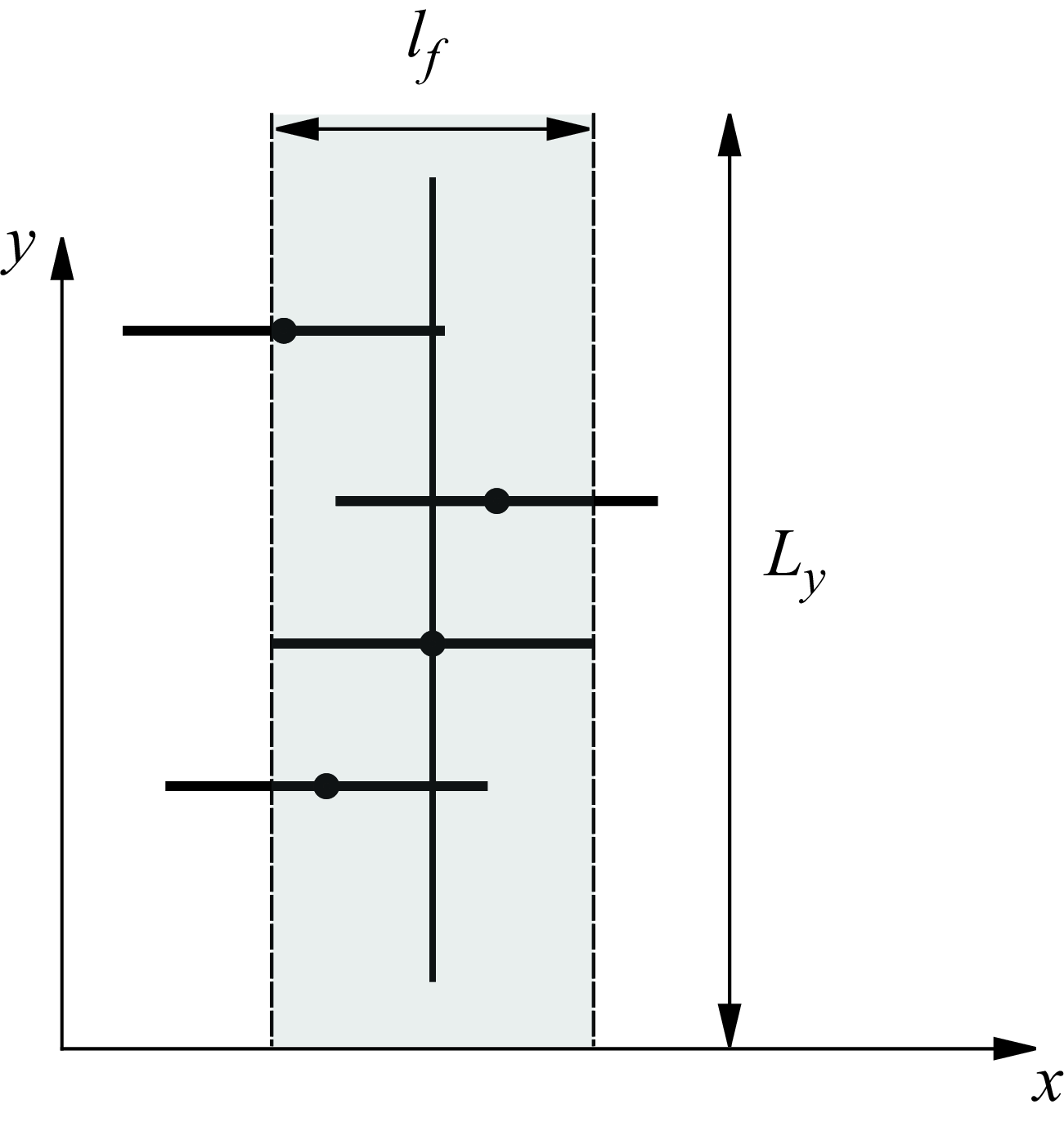
Figure 4. Fractures intersecting with a vertical line of length $L_y$
; the expected number of intersections is
$L_y$
; the expected number of intersections is $N_{\textit{intersection}} = \rho _f l_f L_y$
.
$N_{\textit{intersection}} = \rho _f l_f L_y$
.
Recall the definition of $\bar {g}$
as the transfer coefficient that relates the expected fracture-matrix flow exchange to the expected pressure difference between two points of the respective domains. With the pressure profile from (2.37) the expected flow from a matrix location
$\bar {g}$
as the transfer coefficient that relates the expected fracture-matrix flow exchange to the expected pressure difference between two points of the respective domains. With the pressure profile from (2.37) the expected flow from a matrix location $x$
to fractures with centres at
$x$
to fractures with centres at $x'$
is
$x'$
is
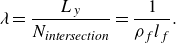
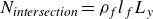
 \begin{align} \bar {q}_{m \to f}(x, x') & = \underbrace {\rho _f}_{\text{number of fractures}} \underbrace {k_m \left(\lim _{y \to 0^+} \left | \frac {\partial p}{\partial y} \right |+\lim _{y \to 0^-} \left | \frac {\partial p}{\partial y} \right | \right)}_{\text{flow rate normal to the fracture-matrix interface}} \nonumber \\ & = 2\rho _f k_m \nabla _x^\infty p (1-C_\lambda )\frac {x-x'}{\lambda }\nonumber \\ & = 2\rho _f^2l_f k_m\nabla _x^\infty p(1-C_\lambda )(x-x'). \end{align}
From (2.40), (2.22) and (2.23), definition (2.24) and by replacing $\nabla _x^\infty p$
with the local approximation
$\nabla _x^\infty p$
with the local approximation
 \begin{align} \nabla _x^\infty p=\frac {p_f(x')-p_m(x)}{x'-x}, \end{align}
one obtains
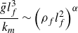
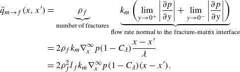
 \begin{align} \bar {g} = \frac {\bar {q}_{m \to f}(x, x')}{\bar {p}_m(x)-\bar {p}_f(x')} = 2\rho _f^2l_f k_m(1-C_\lambda ), \end{align}
or in normalised form
 \begin{align} \frac {\bar {g}l_f^3}{k_m} = 2(1-C_\lambda )(\rho _f l_f^2)^2 \sim (\rho _f l_f^2)^2, \end{align}
with $\alpha = 2$
; see (2.35). Thus to summarise, the parameter
$\alpha = 2$
; see (2.35). Thus to summarise, the parameter $\alpha$
in (2.35) takes two asymptotic values, i.e.
$\alpha$
in (2.35) takes two asymptotic values, i.e. $\alpha \to 1$
for
$\alpha \to 1$
for $\rho _f l_f^2 \to 0$
and
$\rho _f l_f^2 \to 0$
and $\alpha \to 2$
for
$\alpha \to 2$
for $\rho _f l_f^2 \to \infty$
, and the normalised transfer coefficient obeys the following scaling law:
$\rho _f l_f^2 \to \infty$
, and the normalised transfer coefficient obeys the following scaling law:
 \begin{align} \frac {\bar {g}l_f^3}{k_m} \sim \begin{cases} \rho _f l_f^2 & \quad \rho _f l_f^2 \to 0 \\[4pt] (\rho _f l_f^2)^2 & \quad \rho _f l_f^2 \to \infty \end{cases}. \end{align}
Note that for $\rho _f l_f^2 \to 0$
the scaling parameter can be determined from a single fracture simulation and for
$\rho _f l_f^2 \to 0$
the scaling parameter can be determined from a single fracture simulation and for $\rho _f l_f^2 \to \infty$
one derives it analytically, provided
$\rho _f l_f^2 \to \infty$
one derives it analytically, provided $C_\lambda$
is known (for highly conductive fractures
$C_\lambda$
is known (for highly conductive fractures $C_\lambda \to 0$
).
$C_\lambda \to 0$
).
3. Results
3.1. Validation of the scaling law
To validate the scaling law proposed in § 2.3, we performed MCS as described in § 2.1 on a domain of size $L_x \times L_y = 10 \times 5$
, which is discretised into
$L_x \times L_y = 10 \times 5$
, which is discretised into $n_x \times n_y = 1000 \times 500$
cells. Periodic boundary conditions are imposed in both directions, with an enforced pressure difference
$n_x \times n_y = 1000 \times 500$
cells. Periodic boundary conditions are imposed in both directions, with an enforced pressure difference $p_l-p_r=1$
in the
$p_l-p_r=1$
in the $x$
-direction. The fracture aspect ratio
$x$
-direction. The fracture aspect ratio ${(l_f)}/({a_f})$
is kept at
${(l_f)}/({a_f})$
is kept at $10^3$
, the fractures and matrix permeabilities are
$10^3$
, the fractures and matrix permeabilities are $k_f = 10^5$
and
$k_f = 10^5$
and $k_m = 1$
, respectively, the fracture number density
$k_m = 1$
, respectively, the fracture number density $\rho _f$
varies from
$\rho _f$
varies from $10$
to
$10$
to $100$
with stepsize
$100$
with stepsize $10$
, and the fracture length
$10$
, and the fracture length $l_f$
varies from
$l_f$
varies from $0.11$
to
$0.11$
to $1.01$
with stepsize
$1.01$
with stepsize $0.02$
. For each combination of
$0.02$
. For each combination of $\rho _f$
and
$\rho _f$
and $l_f$
,
$l_f$
, $1000$
realisations were simulated to estimate the mean volumetric flow rate
$1000$
realisations were simulated to estimate the mean volumetric flow rate $\bar {u}_f^\infty$
through the fracture domain. Note that from the mean volumetric flow rate the transfer coefficient
$\bar {u}_f^\infty$
through the fracture domain. Note that from the mean volumetric flow rate the transfer coefficient $\bar {g} = {(12)}/{(l_f^3)} |{(\bar {u}_f^\infty)}/{(\nabla _x^\infty p)} |$
can be calculated. Figure 5 shows the normalised transfer coefficient
$\bar {g} = {(12)}/{(l_f^3)} |{(\bar {u}_f^\infty)}/{(\nabla _x^\infty p)} |$
can be calculated. Figure 5 shows the normalised transfer coefficient ${\bar {g}l_f^3}/{k_m}$
against the dimensionless parameter
${\bar {g}l_f^3}/{k_m}$
against the dimensionless parameter $\rho _f l_f^2$
in log-log scale. As expected, two asymptotes can be identified, i.e.
$\rho _f l_f^2$
in log-log scale. As expected, two asymptotes can be identified, i.e.
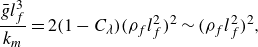
 \begin{align} \text{log}\left (\frac {\bar {g}l_f^3}{k_m}\right ) = \begin{cases} \text{log}(\rho _f l_f^2)+C_1 & \quad \rho _f l_f^2 \to 0 \\ 2\text{log}(\rho _f l_f^2)+C_2 & \quad \rho _f l_f^2 \to \infty , \end{cases} \end{align}
which is consistent with the derived scaling law expressed by (2.44).

Figure 5. Normalised transfer coefficient ${(\bar {g}l_f^3)}/{(k_m)}$
as a function of
${(\bar {g}l_f^3)}/{(k_m)}$
as a function of $\rho _f l_f^2$
in log-log scale; red dots, MCS data; blue curve, fitted hyperbola; black dashed lines, asymptotes
$\rho _f l_f^2$
in log-log scale; red dots, MCS data; blue curve, fitted hyperbola; black dashed lines, asymptotes $\text{log}({(\bar {g}l_f^3)}/{(k_m)}) = \text{log}(\rho _f l_f^2)+C_1$
and
$\text{log}({(\bar {g}l_f^3)}/{(k_m)}) = \text{log}(\rho _f l_f^2)+C_1$
and $\text{log}({\bar {g}l_f^3}/{k_m}) = 2 \text{log}(\rho _f l_f^2)+C_2$
.
$\text{log}({\bar {g}l_f^3}/{k_m}) = 2 \text{log}(\rho _f l_f^2)+C_2$
.
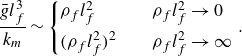
We assume that the transition between the two asymptotes takes the form of a hyperbola:
 \begin{align} & AX^2 + 2BXY + CY^2 + 2DX + 2EY + F = 0 \quad (A\gt 0) \quad \text{or}\nonumber \\ Y & = -\frac {BX+E}{C}+\frac {\sqrt {(BX+E)^2-(AX^2+2DX+F)C}}{C} \end{align}
where $X=\text{log}(\rho _f l_f^2)$
and
$X=\text{log}(\rho _f l_f^2)$
and $Y=\text{log} ({(\bar {g}l_f^3)}/{(k_m)} )$
. The coefficients
$Y=\text{log} ({(\bar {g}l_f^3)}/{(k_m)} )$
. The coefficients $A$
,
$A$
, $B$
and
$B$
and $C$
are determined by the slopes of the asymptotes. To determine
$C$
are determined by the slopes of the asymptotes. To determine $D$
,
$D$
, $E$
and
$E$
and $F$
, at least one DFM simulation with a single fracture in a very large domain and one MCS study with appropriate value of
$F$
, at least one DFM simulation with a single fracture in a very large domain and one MCS study with appropriate value of $\rho _f l_f^2$
are needed. The single fracture simulation, corresponding to the limiting case where
$\rho _f l_f^2$
are needed. The single fracture simulation, corresponding to the limiting case where $\rho _f l_f^2 \to 0$
, fixes a point on the lower asymptote with slope one, and for highly conductive fractures with
$\rho _f l_f^2 \to 0$
, fixes a point on the lower asymptote with slope one, and for highly conductive fractures with $C_\lambda \to 0$
the other asymptote can be obtained analytically as
$C_\lambda \to 0$
the other asymptote can be obtained analytically as ${(\bar {g}l_f^3)}/{(k_m)} = 2(\rho _fl_f^2)^2$
according to (2.43). The MCS is only required for the remaining data point with an intermediate value of
${(\bar {g}l_f^3)}/{(k_m)} = 2(\rho _fl_f^2)^2$
according to (2.43). The MCS is only required for the remaining data point with an intermediate value of $\rho _fl_f^2$
. With these three values, the transfer coefficient can be derived for any combinations of matrix permeability
$\rho _fl_f^2$
. With these three values, the transfer coefficient can be derived for any combinations of matrix permeability $k_m$
, fracture number density
$k_m$
, fracture number density $\rho _f$
and fracture length
$\rho _f$
and fracture length $l_f$
; we found the hyperbola coefficients to be
$l_f$
; we found the hyperbola coefficients to be
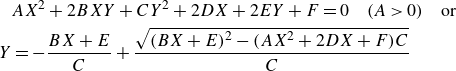
 \begin{align} A & = 0.620,\nonumber \\ B & = -0.465,\nonumber \\ C & = 0.310, \nonumber \\ D & = 0.677,\nonumber \\ E & = -0.364,\nonumber \\ F & = -0.080. \end{align}
Henceforth, in all the following simulations based on our non-local model, $\bar {g}$
is taken from (3.2) with the coefficients from (3.3).
$\bar {g}$
is taken from (3.2) with the coefficients from (3.3).
3.2. Case study: discontinuous fracture statistics
In order to assess the capabilities of the outlined non-local model for spatially varying fracture statistics, the first two test cases with discontinuous changes of the statistics in the middle of the domain were examined. In the first test case, the fracture length is kept constant at $l_f=0.25$
, while the number density
$l_f=0.25$
, while the number density $\rho _f$
is
$\rho _f$
is $10$
and
$10$
and $50$
on the left and right halves of the domain, respectively. In the second test case, the fracture number density is kept constant at
$50$
on the left and right halves of the domain, respectively. In the second test case, the fracture number density is kept constant at $\rho _f = 30$
, but the fracture length
$\rho _f = 30$
, but the fracture length $l_f$
was set to
$l_f$
was set to $0.11$
and
$0.11$
and $0.21$
on the left and right halves of the domain, respectively. In both cases the domain height
$0.21$
on the left and right halves of the domain, respectively. In both cases the domain height $L_y$
is
$L_y$
is $1$
, while the domain length
$1$
, while the domain length $L_x$
varies from
$L_x$
varies from $0.1$
to
$0.1$
to $0.3$
with steps of
$0.3$
with steps of $0.02$
and from
$0.02$
and from $0.3$
to
$0.3$
to $1.5$
with steps of
$1.5$
with steps of $0.1$
. Dirichlet boundary conditions were imposed at the left and right boundaries with
$0.1$
. Dirichlet boundary conditions were imposed at the left and right boundaries with $p_l = 1$
and
$p_l = 1$
and $p_r = 0$
. Reference solutions were obtained with MCS using 1000 independent realisations per test case, each employing a grid resolution of
$p_r = 0$
. Reference solutions were obtained with MCS using 1000 independent realisations per test case, each employing a grid resolution of $h=0.01$
. The model equations (2.22)–(2.25) were solved using the
$h=0.01$
. The model equations (2.22)–(2.25) were solved using the $\bar {g}$
values obtained from the scaling law given by (3.2). The results are presented next and further discussions will follow in § 4. Figure 6 shows the mean pressure profiles of the first case with changing fracture density. The upper and lower rows show the mean pressure profiles in the matrix and fracture domains, respectively, while the three columns correspond to
$\bar {g}$
values obtained from the scaling law given by (3.2). The results are presented next and further discussions will follow in § 4. Figure 6 shows the mean pressure profiles of the first case with changing fracture density. The upper and lower rows show the mean pressure profiles in the matrix and fracture domains, respectively, while the three columns correspond to $L_x\in \{0.3, 0.6, 0.9\}$
(left, middle and right, respectively). Figure 7 shows the mean volumetric flow rates through the domain of the first case. Similarly, mean pressure profiles and mean volumetric flow rates of the second case are shown in figures 8 and 9, respectively.
$L_x\in \{0.3, 0.6, 0.9\}$
(left, middle and right, respectively). Figure 7 shows the mean volumetric flow rates through the domain of the first case. Similarly, mean pressure profiles and mean volumetric flow rates of the second case are shown in figures 8 and 9, respectively.
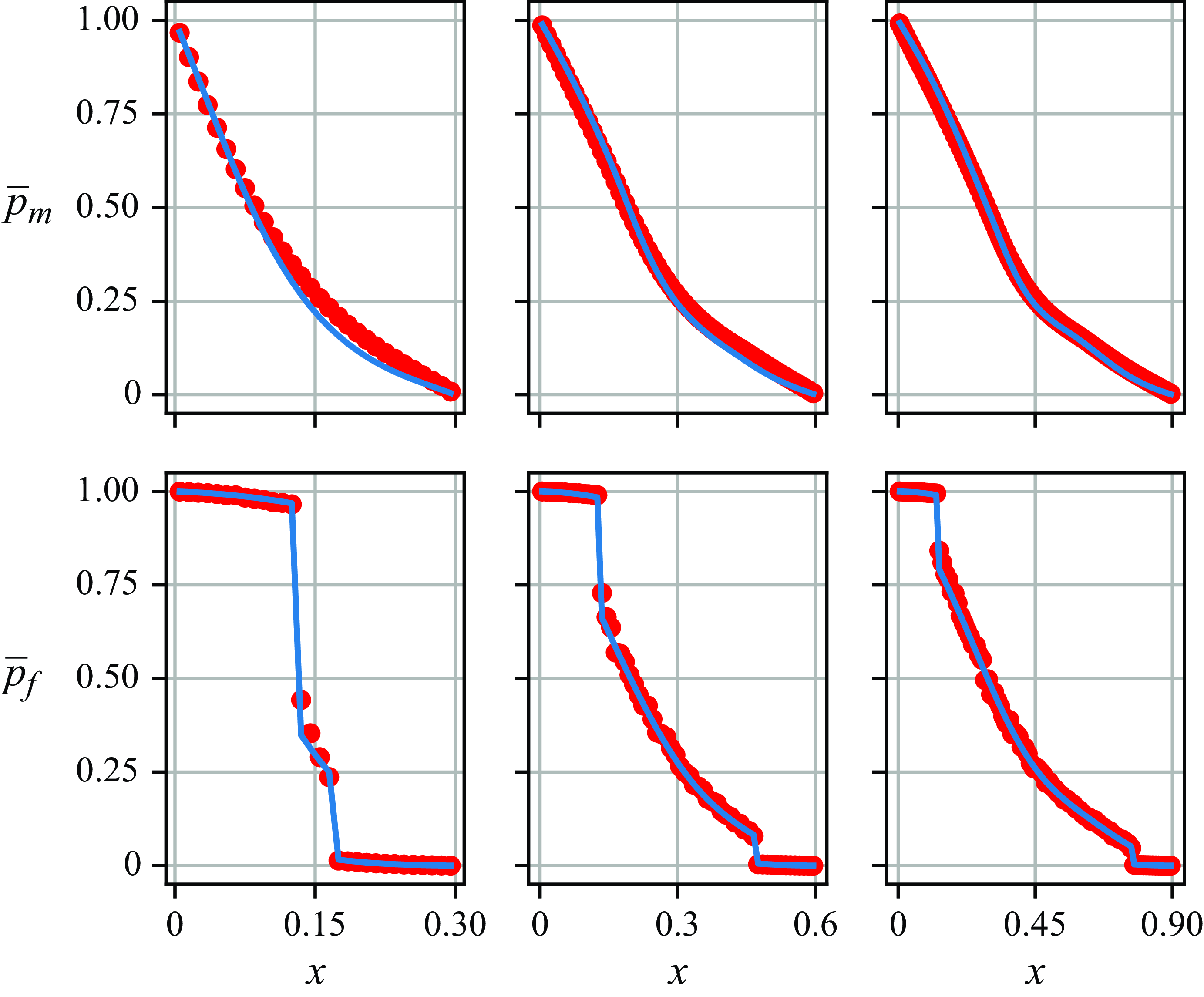
Figure 6. Mean pressure profiles in a fractured porous medium with discontinuous fracture statistics. The fracture number density $\rho _f$
on the left half of the domain is
$\rho _f$
on the left half of the domain is $10$
and on the right half it is
$10$
and on the right half it is $50$
. The upper row shows mean pressure profiles in the matrix domain and the lower row mean pressure profiles in the fracture domain. The three columns correspond to
$50$
. The upper row shows mean pressure profiles in the matrix domain and the lower row mean pressure profiles in the fracture domain. The three columns correspond to $L_x\in \{0.3, 0.6, 0.9\}$
(left, middle and right, respectively). Red dots, MCS data. Blue curves, kernel-based model results.
$L_x\in \{0.3, 0.6, 0.9\}$
(left, middle and right, respectively). Red dots, MCS data. Blue curves, kernel-based model results.
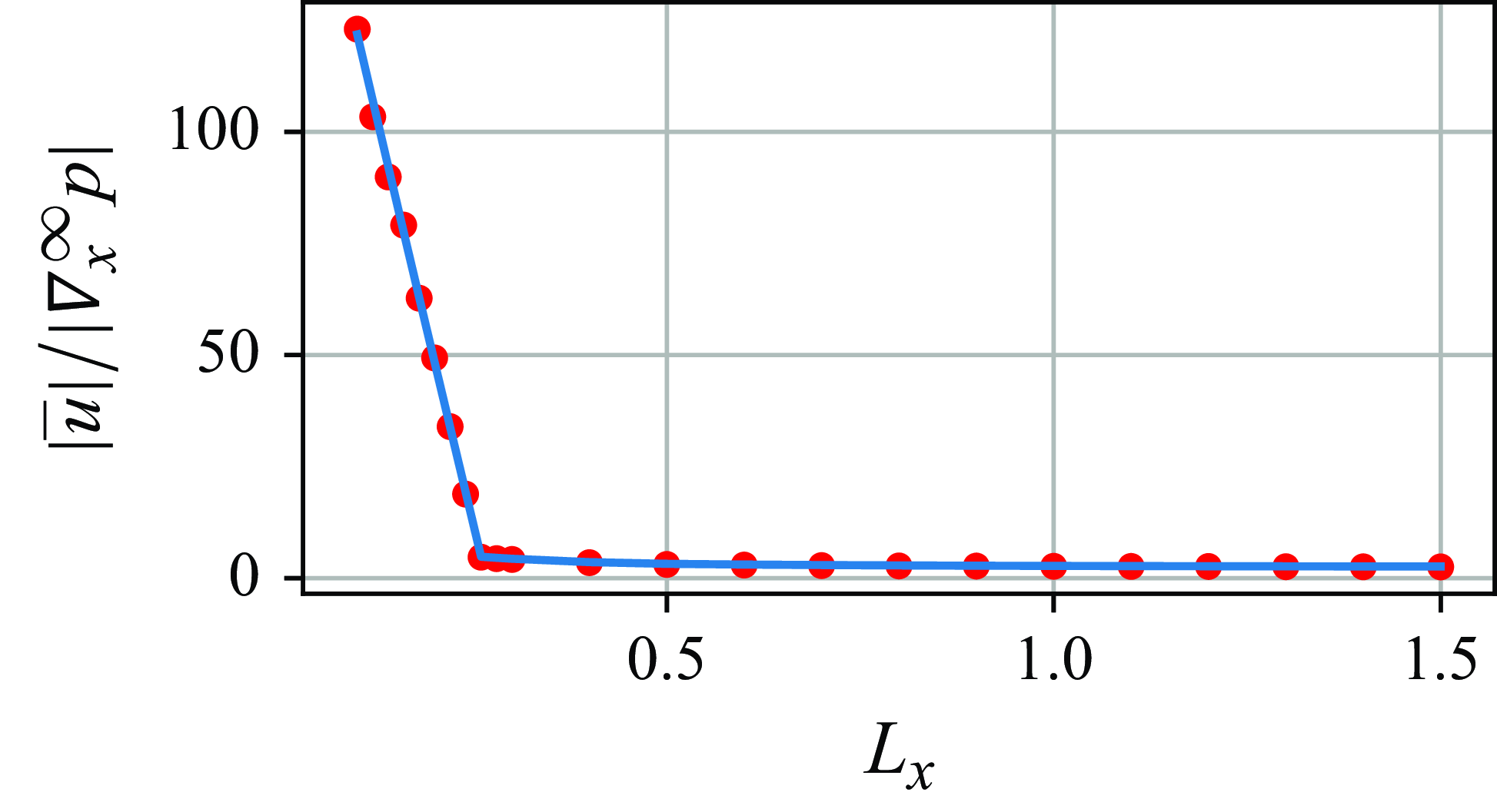
Figure 7. Normalised flow rates through a fractured porous medium with discontinuous fracture statistics. The fracture length $l_f$
on the left half of the domain is
$l_f$
on the left half of the domain is $0.11$
and on the right half is
$0.11$
and on the right half is $0.21$
. Red dots, MCS data. Blue curves, kernel-based model results.
$0.21$
. Red dots, MCS data. Blue curves, kernel-based model results.
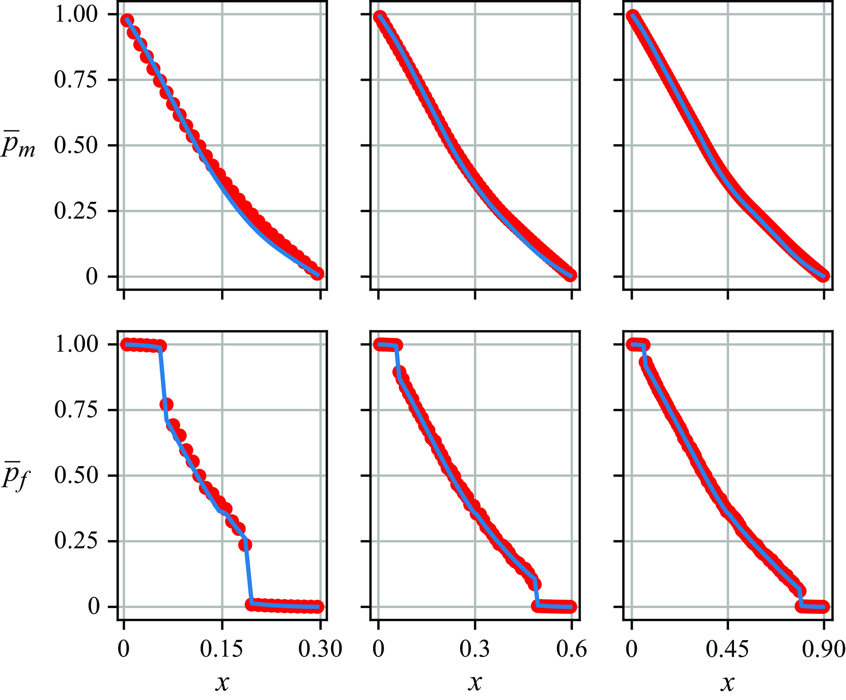
Figure 8. Mean pressure profiles in a fractured porous medium with discontinuous fracture statistics. The fracture length $l_f$
on the left half of the domain is
$l_f$
on the left half of the domain is $0.11$
and on the right half is
$0.11$
and on the right half is $0.21$
. The upper row shows mean pressure profiles in the matrix domain and the lower row mean pressure profiles in the fracture domain. The three columns correspond to
$0.21$
. The upper row shows mean pressure profiles in the matrix domain and the lower row mean pressure profiles in the fracture domain. The three columns correspond to $L_x\in \{0.3, 0.6, 0.9\}$
(left, middle and right, respectively). Red dots, MCS data. Blue curves, kernel-based model results.
$L_x\in \{0.3, 0.6, 0.9\}$
(left, middle and right, respectively). Red dots, MCS data. Blue curves, kernel-based model results.
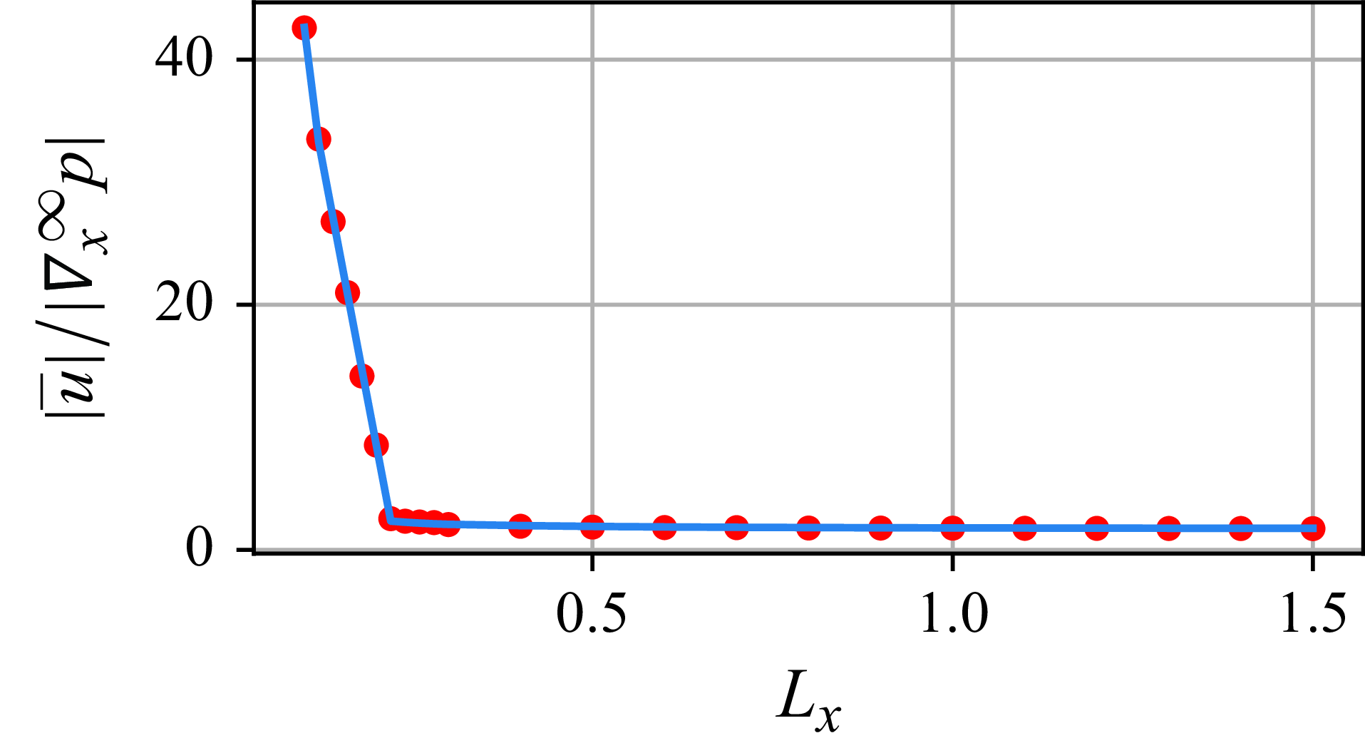
Figure 9. Normalised flow rates through a fractured porous medium with discontinuous fracture statistics. The fracture length $l_f$
on the left half of the domain is
$l_f$
on the left half of the domain is $0.11$
and on the right half is
$0.11$
and on the right half is $0.21$
. Red dots, MCS data. Blue curves, kernel-based model results.
$0.21$
. Red dots, MCS data. Blue curves, kernel-based model results.
3.3. Case study: continuous fracture statistics
In a second study, two test cases with continuously varying fracture statistics are presented. In the first test case, the fracture length is kept constant at $l_f=0.25$
, while the number density
$l_f=0.25$
, while the number density $\rho _f = 50({x}/{L_x})+10$
varies linearly with respect to the
$\rho _f = 50({x}/{L_x})+10$
varies linearly with respect to the $x$
-coordinate. In the second test case, the fracture number density is kept constant at
$x$
-coordinate. In the second test case, the fracture number density is kept constant at $\rho _f=30$
and the fracture length
$\rho _f=30$
and the fracture length
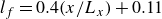
 $l_f = 0.4({x}/{L_x})+0.11$
varies linearly with respect to the
$l_f = 0.4({x}/{L_x})+0.11$
varies linearly with respect to the $x$
-coordinate. All other parameters are the same as for the discontinuous test cases. Figures 10 and 11, respectively, show mean pressure profiles and mean volumetric flow rates for the first continuous test case. Figures 12 and 13 show the same for the second continuous test case.
$x$
-coordinate. All other parameters are the same as for the discontinuous test cases. Figures 10 and 11, respectively, show mean pressure profiles and mean volumetric flow rates for the first continuous test case. Figures 12 and 13 show the same for the second continuous test case.
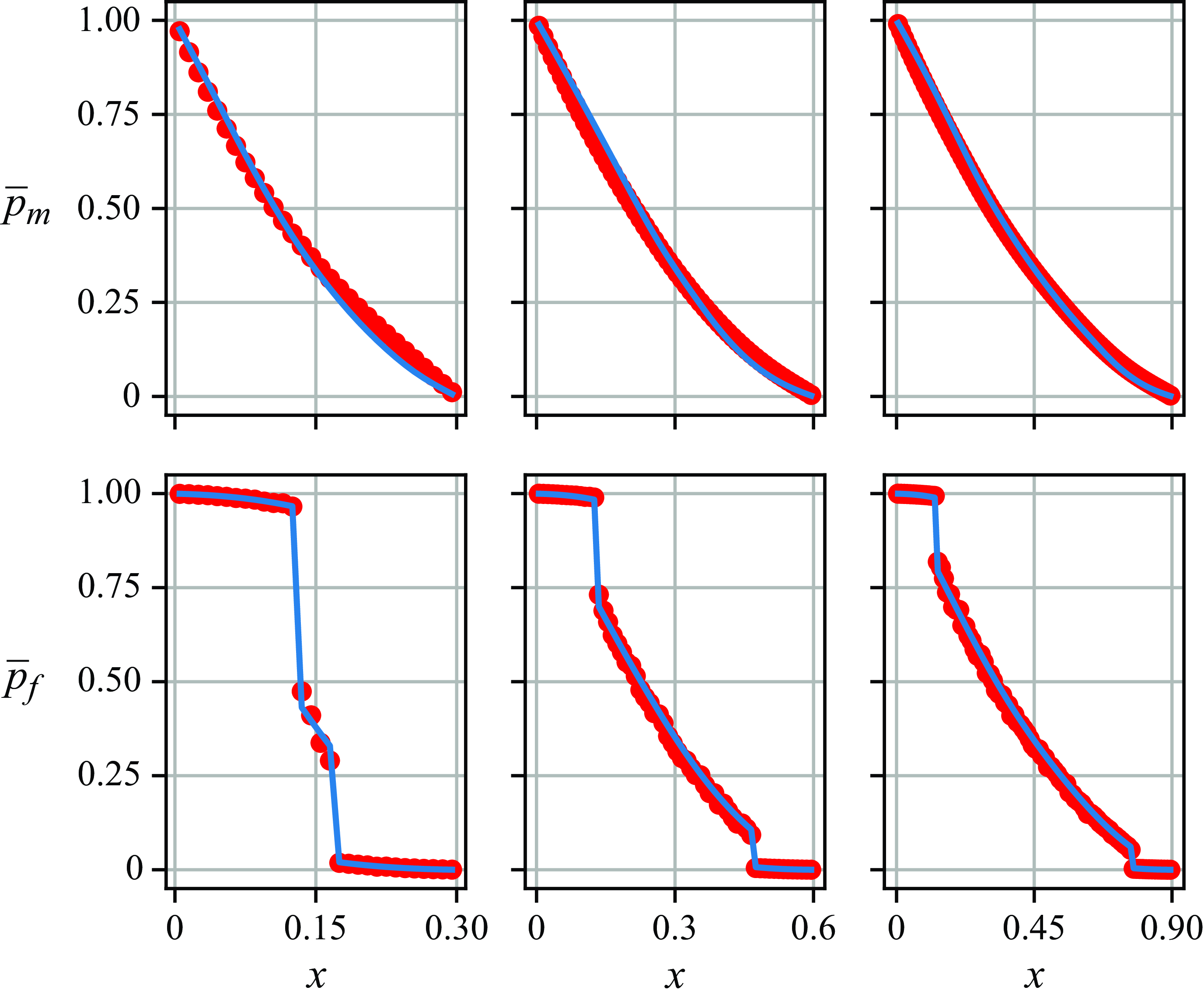
Figure 10. Mean pressure profiles in a fractured porous medium with continuously varying fracture statistics. The fracture number density $\rho _f = 50({x}/{L_x})+10$
varies linearly with respect to the
$\rho _f = 50({x}/{L_x})+10$
varies linearly with respect to the $x$
-coordinate. The upper row shows mean pressure profiles in the matrix domain and the lower row mean pressure profiles in the fracture domain. The three columns correspond to
$x$
-coordinate. The upper row shows mean pressure profiles in the matrix domain and the lower row mean pressure profiles in the fracture domain. The three columns correspond to $L_x\in \{0.3, 0.6, 0.9\}$
(left, middle and right, respectively). Red dots, MCS data. Blue curves, kernel-based model results.
$L_x\in \{0.3, 0.6, 0.9\}$
(left, middle and right, respectively). Red dots, MCS data. Blue curves, kernel-based model results.
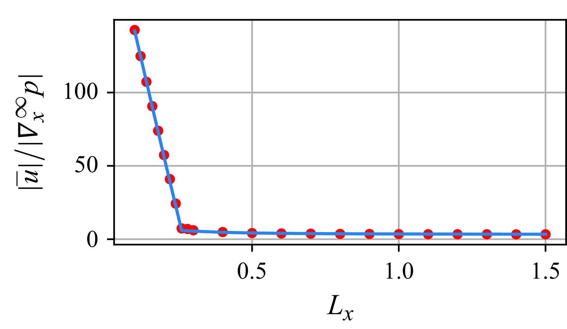
Figure 11. Normalised flow rates through a fractured porous medium with continuously varying fracture statistics. The fracture number density $\rho _f = 50({x}/{L_x})+10$
varies linearly with respect to the
$\rho _f = 50({x}/{L_x})+10$
varies linearly with respect to the $x$
-coordinate. Red dots, MCS data. Blue curves, kernel-based model results.
$x$
-coordinate. Red dots, MCS data. Blue curves, kernel-based model results.
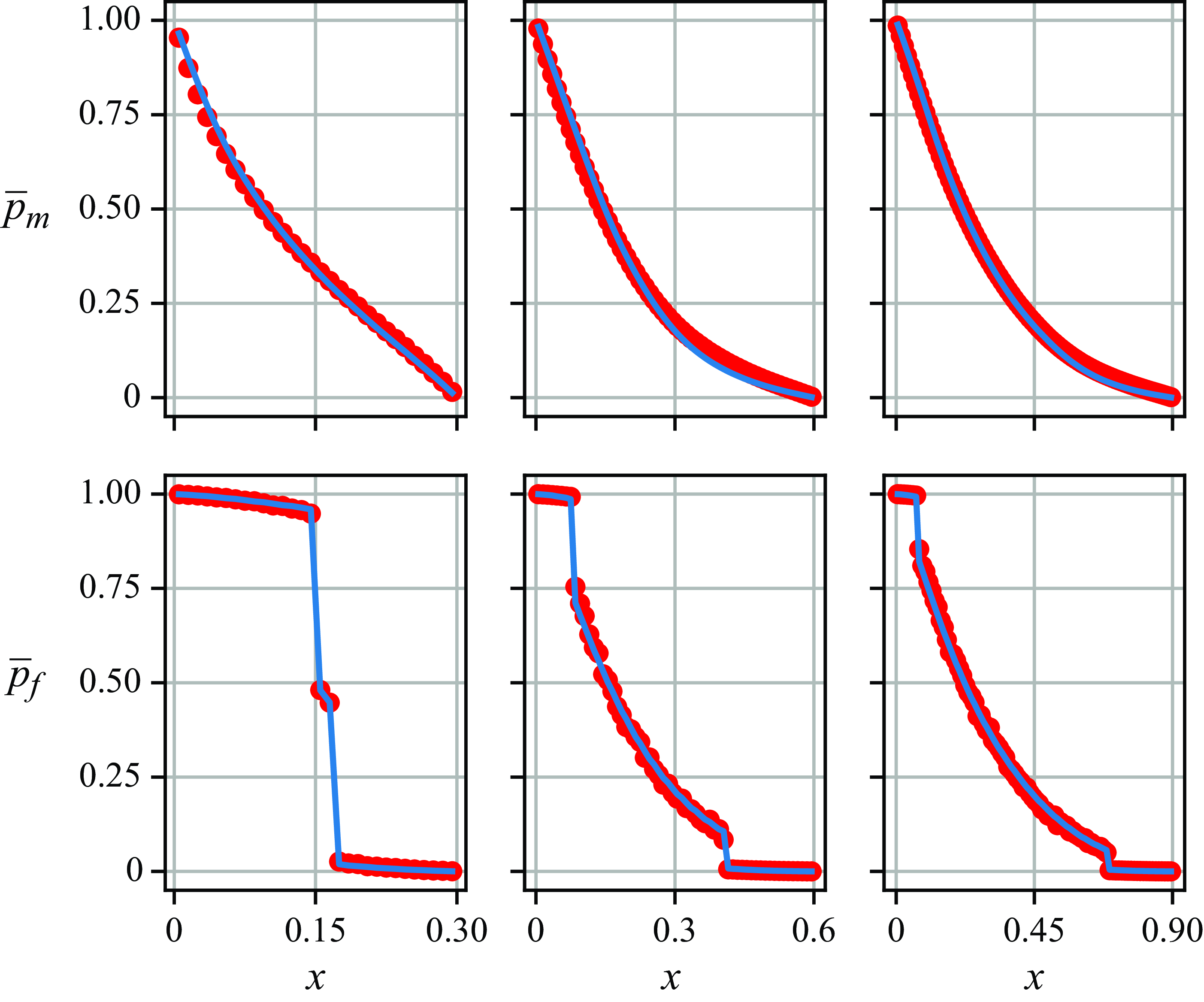
Figure 12. Mean pressure profiles in a fractured porous medium with continuously varying fracture statistics. The fracture length $l_f = 0.4({x}/{L_x})+0.11$
varies linearly with respect to the
$l_f = 0.4({x}/{L_x})+0.11$
varies linearly with respect to the $x$
-coordinate. The upper row shows mean pressure profiles in the matrix domain and the lower row mean pressure profiles in the fracture domain. The three columns correspond to
$x$
-coordinate. The upper row shows mean pressure profiles in the matrix domain and the lower row mean pressure profiles in the fracture domain. The three columns correspond to $L_x\in \{0.3, 0.6, 0.9\}$
(left, middle and right, respectively). Red dots, MCS data. Blue curves, kernel-based model results.
$L_x\in \{0.3, 0.6, 0.9\}$
(left, middle and right, respectively). Red dots, MCS data. Blue curves, kernel-based model results.
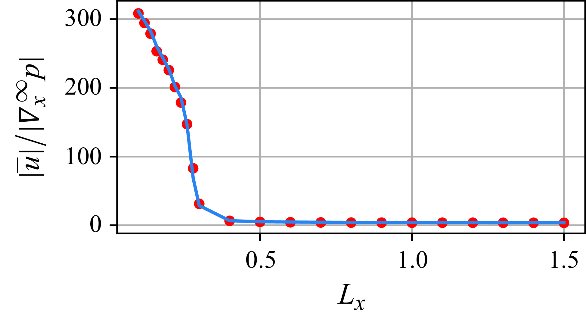
Figure 13. Normalised flow through a fractured porous medium with continuously varying fracture statistics. The fracture length $l_f = 0.4({x}/{L_x})+0.11$
varies linearly with respect to the
$l_f = 0.4({x}/{L_x})+0.11$
varies linearly with respect to the $x$
-coordinate. Red dots, MCS data. Blue curves, kernel-based model results.
$x$
-coordinate. Red dots, MCS data. Blue curves, kernel-based model results.
4. Discussion and conclusions
The results presented in §§ 3.2 and 3.3 show close agreement between model predictions and the MCS reference. This demonstrates that the kernel-based model is capable of simulating flow in fractured porous media with spatially instationary fracture statistics. Moreover, it was found that the transfer coefficient that relates the expected fracture-matrix exchange rate to the expected pressure difference between the two domains only depends on the local fracture statistics. The determination of the transfer coefficient requires the expected volumetric flow in the fracture domain, which is based on one empirical value derived from an MCS study. If the fracture statistics vary continuously, the transfer coefficient becomes a field value, but based on the previously presented scaling analysis it becomes an algebraic function of the local fracture statistics. In the limit of very small fracture number density, the transfer coefficient scales linearly with the number density while in the limit of infinitely large number density – due to the interference between the fractures – the flow exchange across the fracture-matrix boundary is intensified and the transfer coefficient scales quadratically with the number density. To determine the constants in the scaling law, only one single fracture simulation and two MCS studies (one MCS study if the fractures are highly conductive) are needed. With the proposed scaling law, the non-local kernel-based model can be applied to any fractured porous medium with spatially heterogeneous fracture distributions. In the current work statistically one-dimensional test cases were presented, but the model formulation is valid for two- and three-dimensional scenarios as well. Equations (2.22) and (2.23) represent a simplified formulation as opposed to (3.1), (3.2), (3.3) in the last author’s previous work (Jenny Reference Jenny2020), where the conceptual incorporation of percolated fracture networks was also outlined. To increase the real-world applicability of the model, extensions involving tilted fractures, fracture clusters as well as percolated fracture networks are planned. While preparatory work in connection with percolated fracture networks has been included in the previous study (Jenny Reference Jenny2020), the generalisation to two- and three-dimensional configurations in connection with tilted fractures will be challenging.
Funding
This research received no specific grant from any funding agency, commercial or not-for-profit sectors.
Declaration of interests
The authors report no conflict of interest.


 Open access