


1. Introduction
Many systems of multi-scale differential equations undergo dynamic Hopf bifurcations in which a parameter slowly changes and a stable state becomes unstable due to the slow, generic passage of a pair of eigenvalues through the imaginary axis. When the governing equations in the multi-scale (or fast–slow) systems are analytic ordinary differential equations (ODEs), it has been known for over 50 years that there are delays in the onset of the instabilities [Reference Baer, Erneux and Rinzel4, Reference Hayes, Kaper, Szmolyan and Wechselberger20, Reference Neishtadt35–Reference Neishtadt and Treschev39, Reference Shishkova44–Reference Su, Jones and Khibnik47]. Solutions that have approached the stable (attracting) states before the instantaneous Hopf bifurcations remain near those states long after they have become unstable (repelling) in the dynamic Hopf bifurcations. This phenomenon is known as delayed Hopf bifurcation (DHB).
A primary dynamic manifestation of DHB is that the onset of the post-Hopf oscillations is a hard onset, with the systems transitioning rapidly to large-scale oscillations when they leave neighbourhoods of the unstable states. This contrasts with the gradual square root growth of the oscillation amplitudes in generic classical Hopf bifurcations.
Applications of DHBs in ODE models have been studied in many areas of science and engineering: chemistry [Reference Berthier, Diard and Nugues8, Reference Koper28, Reference Koper and Aguda29, Reference Strizhak and Menzinger45], electrical circuits [Reference Han, Xia, Ji, Bi and Kurths19, Reference Holden and Erneux22, Reference Wu, Ye, Chen, Xu and Bao49], electrocardiac models [Reference Kügler30], fluid mechanics and geophysics [Reference Ashwin, Wieczorek, Vitolo and Cox2, Reference Engler, Kaper, Kaper and Vo14, Reference Higuera, Porter and Knobloch21, Reference Maasch and Saltzman32], mechanical oscillators [Reference Braaksma11, Reference Neishtadt and Sidorenko38], neuroscience [Reference Baer, Erneux and Rinzel4, Reference Barreto and Cressman5, Reference Bertram, Butte, Kiemel and Sherman9, Reference Bilinsky and Baer10, Reference Kakiuchi and Tchizawa24, Reference Rinzel and Baer42, Reference Rubin, Terman and Fiedler43, Reference Su46] and economics [Reference Grasman and Wentzel18], among others. For each of these models, the long delay between the instantaneous bifurcation and the onset of oscillations, which is $\mathcal {O}(1/\varepsilon )$
in the fast time (where
$\mathcal {O}(1/\varepsilon )$
in the fast time (where $\varepsilon $
is the small parameter measuring the time-scale separation), plays an important role in the system dynamics.
$\varepsilon $
is the small parameter measuring the time-scale separation), plays an important role in the system dynamics.
Recently, it has been shown that the DHB phenomenon occurs not only in analytic ODEs but also naturally in one-dimensional, multi-scale partial differential equations (PDEs) of reaction–diffusion type [Reference Goh, Kaper and Vo17, Reference Kaper and Vo25]. The phenomenon is governed by a super-critical Hopf bifurcation occurring in the family of fast subsystems parametrized by a slowly varying parameter. Examples studied in [Reference Goh, Kaper and Vo17, Reference Kaper and Vo25] include the complex Ginzburg–Landau equation, the FitzHigh–Nagumo PDE, and the Hodgkin–Huxley PDE. Additional theory for problems with spectral gaps is given in [Reference Avitabile, Desroches, Veltz and Wechselberger3].
In this paper, we show that the phenomenon of DHB also occurs in a pair of multi-scale reaction–diffusion PDEs in two space dimensions. In particular, we study DHBs in the complex Ginzburg–Landau (CGL) PDE in two dimensions and in the Brusselator model in two dimensions. Both of these equations have Hopf bifurcations in which an attracting quasi-steady state (QSS) becomes a repelling QSS, and we consider the problems in which the bifurcation parameters slowly and generically pass through the Hopf points.
First, we use asymptotic analysis on the linearized CGL PDE in two dimensions to show that solutions that approach the attracting QSS before the instantaneous Hopf bifurcation remain close to it even after it has become repelling in the Hopf bifurcation. From the asymptotic analysis, we find that the delays between the time of the instantaneous Hopf bifurcation and the onset of the post-Hopf oscillations are long ( $\mathcal {O}(1/\varepsilon )$
in the fast time) and generally spatially dependent.
$\mathcal {O}(1/\varepsilon )$
in the fast time) and generally spatially dependent.
Next, we quantify the duration of these delays. We define spatio-temporal buffer surfaces and spatio-temporal memory surfaces in the three-dimensional space-time of the CGL PDE. These are the surfaces along which the amplitudes of the particular and homogeneous solutions of the linearized CGL PDE, respectively, cross a threshold, and cause the solution of the full PDE to diverge from the repelling QSS. We derive asymptotic formulas for both surfaces, and we determine how they depend on the initial data and on the properties of the source terms in the CGL PDE. We find that, at each point $(x,y)$
in the domain, numerically computed solutions of the fully nonlinear CGL PDE with initial data given before the Hopf point stay close to the repelling QSS until they reach the spatio-temporal memory surface or the spatio-temporal buffer surface; whichever occurs first at that point. Hence, the linear terms appear to drive the phenomena of DHB in these PDEs, just as they do in the analytic ODEs.
$(x,y)$
in the domain, numerically computed solutions of the fully nonlinear CGL PDE with initial data given before the Hopf point stay close to the repelling QSS until they reach the spatio-temporal memory surface or the spatio-temporal buffer surface; whichever occurs first at that point. Hence, the linear terms appear to drive the phenomena of DHB in these PDEs, just as they do in the analytic ODEs.
We use the label “buffer” for the spatio-temporal buffer surfaces, because no matter how far in the distant past the data is given (that is, how large negative $\mu _0$
is) the solution must leave the neighbourhood of the repelling QSS at the spatio-temporal buffer surface since the attracting QSS also leaves the neighbourhood then. In addition, we use the label “memory” for the spatio-temporal memory surface, because although the memory of the initial data fades quickly after the initial time due to the rapid, exponential contraction toward the attracting QSS, the memory of the data is not lost. On the contrary, the component of the solution given by the initial data re-emerges in a spatially dependent manner when the slowly varying parameter reaches the memory surface to leading order. This terminology is consistent with that commonly used for DHBs in ODEs.
$\mu _0$
is) the solution must leave the neighbourhood of the repelling QSS at the spatio-temporal buffer surface since the attracting QSS also leaves the neighbourhood then. In addition, we use the label “memory” for the spatio-temporal memory surface, because although the memory of the initial data fades quickly after the initial time due to the rapid, exponential contraction toward the attracting QSS, the memory of the data is not lost. On the contrary, the component of the solution given by the initial data re-emerges in a spatially dependent manner when the slowly varying parameter reaches the memory surface to leading order. This terminology is consistent with that commonly used for DHBs in ODEs.
Finally, we present numerical simulations showing that DHB also occurs in the Brusselator PDE model in two dimensions. Since its creation [Reference Prigogine and Lefever41], the Brusselator has served as a prototypical model in pattern formation and chemical oscillation theory (see, for example, [Reference Epstein and Pojman15]). Here, we consider the case when the main bifurcation parameter slowly passes through the Hopf point. As with the CGL PDE, solutions of the Brusselator PDE that approach the attracting QSS before the instantaneous Hopf bifurcation remain near the QSS for long times after it has become repelling. We find that there is a substantial—generally point dependent—delay before the onset of oscillations occurs.
The asymptotic and numerical results that we present here for these prototypical pattern-forming systems in two dimensions extend our earlier work on DHBs in PDEs in one dimension [Reference Goh, Kaper and Vo17, Reference Kaper and Vo25]. In particular, in [Reference Goh, Kaper and Vo17] we defined buffer curves and memory curves for the linearized CGL PDE in one dimension and derived asymptotic formulas for their spatio-temporal dependence. We showed that key terms in the particular solution are exponentially small up until the spatio-temporal buffer curve, and that precisely along it these terms become $\mathcal {O}(1)$
. Similarly, the homogeneous solution is exponentially small up until the memory curve and large after that. Overall, for the CGL PDE in one dimension, we showed that there is a competition between these exponentially small terms: at each point in the one-dimensional domain the term that ceases being small first determines the length of the delay to leading order at that point, and hence also when the hard onset of the (post-Hopf) oscillations occurs. The memory and buffer surfaces defined in this article play a similar role for the CGL PDE in two dimensions.
$\mathcal {O}(1)$
. Similarly, the homogeneous solution is exponentially small up until the memory curve and large after that. Overall, for the CGL PDE in one dimension, we showed that there is a competition between these exponentially small terms: at each point in the one-dimensional domain the term that ceases being small first determines the length of the delay to leading order at that point, and hence also when the hard onset of the (post-Hopf) oscillations occurs. The memory and buffer surfaces defined in this article play a similar role for the CGL PDE in two dimensions.
We recall that classical Hopf bifurcations are ubiquitous in PDEs and spatially extended systems in two dimensions. General results are presented, for example, in [Reference van Saarloos48]. Some specific examples include electrodeposition models [Reference Lacitignola, Bozzini and Sgura31], bulk-surface reaction–diffusion [Reference Paquin-Lefebvre, Nagata and Ward40] and nematic liquid crystals [Reference Dangelmayr and Oprea12, Reference Dangelmayr and Oprea13], in addition to the CGL and Brusselator models studied here.
This paper is organized as follows. In Section 2, we present the main asymptotic analysis to show that DHB occurs in the linearized CGL equation with a slowly varying parameter in two space dimensions. In Section 3, we derive the asymptotic formulas for the spatio-temporal buffer surface and the memory surface for the CGL PDE. In Section 4, we present the results of numerical simulations for the fully nonlinear CGL equation that complement the theoretical predictions (of the previous two sections) for the spatio-temporal dependence of the delayed Hopf bifurcations. Section 5 features the DHB results obtained from numerical simulations of the Brusselator model in two dimensions. Conclusions are presented in Section 6. Some asymptotic calculations are presented in Appendix A.
2. Analysis of DHB in the two-dimensional CGL equation
In two space dimensions, the CGL equation with a source term and a slowly varying parameter is given by
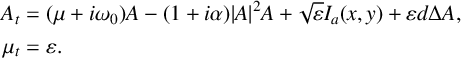 $$ \begin{align} \begin{aligned} A_t &= (\mu + i \omega_0) A - (1+i\alpha)\vert A\vert^2 A + \sqrt{\varepsilon} I_a (x,y) + \varepsilon d \Delta A, \\ \mu_t &= \varepsilon. \end{aligned} \end{align} $$
Here, $(x,y) \in \mathbf {R}^2$
,
$(x,y) \in \mathbf {R}^2$
, $\Delta = {\partial ^2}/{\partial x^2} + {\partial ^2}/{\partial y^2}$
,
$\Delta = {\partial ^2}/{\partial x^2} + {\partial ^2}/{\partial y^2}$
, $t \ge 0$
,
$t \ge 0$
, $A = A(x,y,t)$
is complex valued, and
$A = A(x,y,t)$
is complex valued, and $0< \varepsilon \ll 1$
is a small parameter. The linear growth rate
$0< \varepsilon \ll 1$
is a small parameter. The linear growth rate $\mu = \mu (t)$
is real for the main phenomena we study. The other system parameters satisfy that
$\mu = \mu (t)$
is real for the main phenomena we study. The other system parameters satisfy that $\omega _0>0$
,
$\omega _0>0$
, $\alpha $
is real and d may be complex valued (
$\alpha $
is real and d may be complex valued ( $d = d_R+i d_I$
) with
$d = d_R+i d_I$
) with $d_R>0$
, and these parameters are all independent of
$d_R>0$
, and these parameters are all independent of $\varepsilon $
. The source term
$\varepsilon $
. The source term $I_a(x,y)$
breaks the symmetry
$I_a(x,y)$
breaks the symmetry $ A \to A e^{i\theta }$
for any real
$ A \to A e^{i\theta }$
for any real $\theta $
of the CGL equation and is taken to be bounded and positive, with uniformly bounded derivatives. The initial data at
$\theta $
of the CGL equation and is taken to be bounded and positive, with uniformly bounded derivatives. The initial data at $\mu (0)=\mu _0 < 0$
is
$\mu (0)=\mu _0 < 0$
is $A(x,y,0)=A_0(x,y)$
, and taken to be bounded and continuous for all
$A(x,y,0)=A_0(x,y)$
, and taken to be bounded and continuous for all $(x,y)$
. We refer to [Reference Aranson and Kramer1] for the classical CGL PDE.
$(x,y)$
. We refer to [Reference Aranson and Kramer1] for the classical CGL PDE.
2.1. The attracting and repelling QSSs
The PDE (2.1) has an attracting QSS for all $\mu < -\delta $
, where
$\mu < -\delta $
, where $\delta>0$
is small and
$\delta>0$
is small and $\mathcal {O}(1)$
with respect to
$\mathcal {O}(1)$
with respect to $\varepsilon $
, and solutions approach it at an exponential rate. Similarly, it has a repelling QSS for all
$\varepsilon $
, and solutions approach it at an exponential rate. Similarly, it has a repelling QSS for all $\mu> \delta $
, from which solutions diverge at an exponential rate. These QSS are given by
$\mu> \delta $
, from which solutions diverge at an exponential rate. These QSS are given by
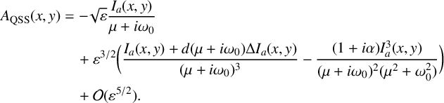 $$ \begin{align} A_{\mathrm{QSS}} (x,y) &= - \sqrt{\varepsilon} \frac{I_a(x,y)}{\mu+i\omega_0} \nonumber\\ &\quad+ \varepsilon^{{3}/{2}} \bigg( \frac{I_a (x,y)+d(\mu+i\omega_0)\Delta I_a(x,y)}{(\mu+i \omega_0)^3} -\frac{(1+i\alpha)I_a^3(x,y)}{(\mu+i\omega_0)^2(\mu^2+\omega_0^2)} \bigg) \nonumber \\ &\quad+ \mathcal{O}(\varepsilon^{{5}/{2}}). \end{align} $$
Here, the $\mathcal {O}(\varepsilon ^{{5}/{2}})$
terms depend on
$\mathcal {O}(\varepsilon ^{{5}/{2}})$
terms depend on $(x,y)$
and
$(x,y)$
and $\mu $
.
$\mu $
.
2.2. Solution of the linearized equation
In this section, we consider $\mu _0<0$
and solve the linearized equation,
$\mu _0<0$
and solve the linearized equation,
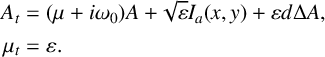 $$ \begin{align*} \begin{aligned} A_t &= (\mu + i \omega_0) A + \sqrt{\varepsilon} I_a (x,y) + \varepsilon d \Delta A,\\ \mu_t &= \varepsilon. \end{aligned} \end{align*} $$
This equation may be simplified using an integrating factor. Let $B(x,y,\mu )=A(x,y,\mu )e^{{-(\mu + i \omega _0)^2}/{2\varepsilon }}$
. The equation for B is an inhomogeneous heat equation,
$B(x,y,\mu )=A(x,y,\mu )e^{{-(\mu + i \omega _0)^2}/{2\varepsilon }}$
. The equation for B is an inhomogeneous heat equation,
 $$ \begin{align} \sqrt{\varepsilon} B_\mu = \sqrt{\varepsilon}d \Delta B + I_a(x,y) e^{{-(\mu+i\omega_0)^2}/{2\varepsilon}}. \end{align} $$
The solution of (2.3) with initial data $B(x,y,\mu _0)=A_0(x,y)e^{{-(\mu _0+i\omega _0)^2}/{2\varepsilon }}$
is obtained by superimposing the homogeneous solution
$B(x,y,\mu _0)=A_0(x,y)e^{{-(\mu _0+i\omega _0)^2}/{2\varepsilon }}$
is obtained by superimposing the homogeneous solution $B_h(x,y,\mu )$
and the particular solution
$B_h(x,y,\mu )$
and the particular solution $B_p(x,y,\mu )$
. For
$B_p(x,y,\mu )$
. For $\mu> \mu _0$
, we find
$\mu> \mu _0$
, we find
 $$ \begin{align*} B_h(x,y,\mu) = \frac{e^{{-(\mu_0+i\omega_0)^2}/{2\varepsilon}}}{4\pi d (\mu-\mu_0)} \int_{\mathbf{R}^2} \textrm{exp} \bigg[ \frac{-(x-x')^2 - (y-y')^2}{4d(\mu - \mu_0)} \bigg] A_0(x',y')\,dx'\,dy'. \end{align*} $$
Here, we have used the fundamental solution of the heat equation in two dimensions,
 $$ \begin{align*} \Phi(x,y,\mu)=\frac{1}{4\pi d \mu}e^{({-(x^2 + y^2)})/{4d\mu}}. \end{align*} $$
Also, for $\mu> \mu _0$
,
$\mu> \mu _0$
,
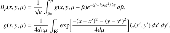 $$ \begin{align*} \begin{split} B_p(x,y,\mu) &= \frac{1}{\sqrt{\varepsilon}} \int_{\mu_0}^\mu g(x,y,\mu-\tilde{\mu}) e^{{-(\tilde{\mu} + i \omega_0)^2}/{2\varepsilon}}\,d\tilde{\mu}, \\ g(x,y,\mu) &= \frac{1}{4d\pi\mu} \int_{\mathbf{R}^2} \mathrm{exp}\bigg[ \frac{-(x-x')^2 - (y-y')^2}{4d\mu}\bigg] I_a(x',y')\,dx'\,dy'. \end{split} \end{align*} $$
Transforming back to the original dependent variable using the integrating factor, we find that, for $\mu> \mu _0$
, the homogeneous solution is
$\mu> \mu _0$
, the homogeneous solution is
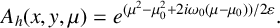
 $$ \begin{align} A_h(x,y,\mu) = \frac{e^{(\mu^2 - \mu_0^2 + 2i \omega_0(\mu-\mu_0))/2\varepsilon}}{4\pi d (\mu-\mu_0)} \int_{\mathbf{R}^2} e^{({-(x-x')^2 - (y-y')^2})/({4d(\mu - \mu_0)})} A_0(x',y')\,dx'\,dy'. \end{align} $$
Furthermore, for $\mu> \mu _0$
, the particular solution is
$\mu> \mu _0$
, the particular solution is
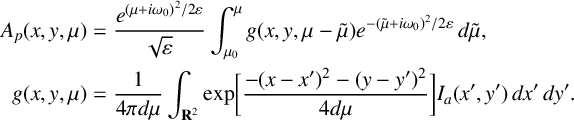 $$ \begin{align*} \begin{aligned} A_p(x,y,\mu) &= \frac{e^{(\mu+i\omega_0)^2/2\varepsilon}}{\sqrt{\varepsilon}} \int_{\mu_0}^\mu g(x,y,\mu-\tilde{\mu}) e^{{-(\tilde{\mu} + i \omega_0)^2}/{2\varepsilon}}\,d\tilde{\mu}, \nonumber \\ g(x,y,\mu) &= \frac{1}{4\pi d\mu} \int_{\mathbf{R}^2} \mathrm{exp}\bigg[ \frac{-(x-x')^2 - (y-y')^2}{4d\mu}\bigg] I_a(x',y')\,dx'\,dy'. \end{aligned} \end{align*} $$
This completes the derivation of the solution of the linearized equation. We calculate $A_h$
for several different types of initial data
$A_h$
for several different types of initial data $A_0(x,y)$
in Section 3.1, and we calculate
$A_0(x,y)$
in Section 3.1, and we calculate $A_p$
for several different types of source terms in Section 3.2. Also, we observe here that it will be useful to distinguish between initial data
$A_p$
for several different types of source terms in Section 3.2. Also, we observe here that it will be useful to distinguish between initial data $A_0(x,y)$
given for
$A_0(x,y)$
given for $\mu _0\le -\omega _0$
and for
$\mu _0\le -\omega _0$
and for $-\omega _0 < \mu _0 < 0$
.
$-\omega _0 < \mu _0 < 0$
.
2.3. Solutions stay near the repelling QSS at least until $\mu =\omega _0$

In this section, we consider solutions with $\mu _0 \le -\omega _0$
. We show that not only do the solutions of (2.1) with
$\mu _0 \le -\omega _0$
. We show that not only do the solutions of (2.1) with $\mu _0\le -\omega _0$
remain close to the attracting QSS until the time of the instantaneous Hopf bifurcation at
$\mu _0\le -\omega _0$
remain close to the attracting QSS until the time of the instantaneous Hopf bifurcation at $\mu =0$
, but after the parameter crosses the instantaneous Hopf bifurcation they remain close to the repelling QSS as well, at least until the time
$\mu =0$
, but after the parameter crosses the instantaneous Hopf bifurcation they remain close to the repelling QSS as well, at least until the time $\mu =+\omega _0$
at all points
$\mu =+\omega _0$
at all points $(x,y)$
for the functions
$(x,y)$
for the functions $I_a(x,y)$
we consider.
$I_a(x,y)$
we consider.
We consider complex values of $\mu $
in a horizontal strip with mid-line on the real axis and of sufficient height (at least
$\mu $
in a horizontal strip with mid-line on the real axis and of sufficient height (at least $3\omega _0$
). This enables the use of classical methods of stationary phase and steepest descents (see, for example, [Reference Bender and Orszag6, Reference Kevorkian and Cole26, Reference Murray34]) to calculate
$3\omega _0$
). This enables the use of classical methods of stationary phase and steepest descents (see, for example, [Reference Bender and Orszag6, Reference Kevorkian and Cole26, Reference Murray34]) to calculate $A_p(x,y,\mu )$
. We find, for
$A_p(x,y,\mu )$
. We find, for $\delta \le \mu \le \omega _0$
,
$\delta \le \mu \le \omega _0$
,
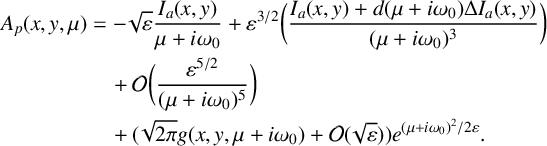 $$ \begin{align} A_p(x,y,\mu)&= - \sqrt{\varepsilon} \frac{I_a(x,y)}{\mu + i \omega_0}+ \varepsilon^{{3}/{2}} \bigg( \frac{I_a(x,y)+d(\mu+i\omega_0)\Delta I_a(x,y)} {(\mu+i \omega_0)^3} \bigg) \nonumber \\ &\quad + \mathcal{O}\bigg(\frac{\varepsilon^{{5}/{2}}}{(\mu+i\omega_0)^5}\bigg)\nonumber \\ &\quad + ( \sqrt{2\pi} g(x,y,\mu+i\omega_0) +\mathcal{O}(\sqrt{\varepsilon}) ) e^{(\mu+i\omega_0)^2/2\varepsilon}. \end{align} $$
The calculation is presented in Appendix A.
The first and second terms are precisely the leading-order terms in the expansion of the repelling QSS for the linear CGL (compare with (2.2), where the QSSs are given for the cubic CGL equation). The third (remainder) term contains the higher-order terms in the asymptotic expansion of the repelling QSS, and continued integration by parts will yield them. The fourth term is exponentially small for $\mu \in [\delta ,\omega _0 -K\varepsilon ^r)$
, for some
$\mu \in [\delta ,\omega _0 -K\varepsilon ^r)$
, for some $K>0$
and any
$K>0$
and any $0<r<1$
. It is a classic Stokes-type term. This term is not in the expansion of the repelling QSS (on
$0<r<1$
. It is a classic Stokes-type term. This term is not in the expansion of the repelling QSS (on $\mu>\delta $
) to all orders. Rather, it is beyond all orders,
$\mu>\delta $
) to all orders. Rather, it is beyond all orders, $\mathcal {O}(e^{-{\omega _0^2}/{2\varepsilon }})$
, arising naturally from tracking solutions on (and near) the attracting QSS along a contour over the saddle point in the complex
$\mathcal {O}(e^{-{\omega _0^2}/{2\varepsilon }})$
, arising naturally from tracking solutions on (and near) the attracting QSS along a contour over the saddle point in the complex $\mu $
plane and into the regime of
$\mu $
plane and into the regime of $\mathrm {Re} (\mu )>0$
. It is a measure of the exponentially small distance between the attracting and repelling QSS at
$\mathrm {Re} (\mu )>0$
. It is a measure of the exponentially small distance between the attracting and repelling QSS at $\mu =0$
.
$\mu =0$
.
Overall, formula (2.5) shows that, at all points $(x,y)$
, the solutions of the linear CGL equation with Gevrey regular data
$(x,y)$
, the solutions of the linear CGL equation with Gevrey regular data $A_0(x,y)$
given at
$A_0(x,y)$
given at $\mu _0 \le -\omega _0$
remain near the repelling QSS at least until
$\mu _0 \le -\omega _0$
remain near the repelling QSS at least until $\mu = \omega _0$
to leading order.
$\mu = \omega _0$
to leading order.
Next, one also needs to include the nonlinear terms from (2.1). This was done for DHB in the one-dimensional CGL PDE in Section 6 of [Reference Goh, Kaper and Vo17]. There, we first used the same type of integrating factor (as used in (2.3) above) to rewrite the nonlinear PDE for $B(x,\mu )$
. Then, we split the solution into two parts:
$B(x,\mu )$
. Then, we split the solution into two parts: $B(x,\mu ) = B_p(x,\mu ) + b(x,\mu )$
, where we recall that
$B(x,\mu ) = B_p(x,\mu ) + b(x,\mu )$
, where we recall that $B_p$
is the particular solution of the linearized equation. The PDE for the remainder term
$B_p$
is the particular solution of the linearized equation. The PDE for the remainder term $b(x,\mu )$
was converted into an integral equation. We showed formally that there is a mild solution of that integral equation, using an iterative method, and that the magnitude of
$b(x,\mu )$
was converted into an integral equation. We showed formally that there is a mild solution of that integral equation, using an iterative method, and that the magnitude of $b(x,\mu )$
remains small at least until
$b(x,\mu )$
remains small at least until $\mu =\omega _0$
. Hence, the solution of the full nonlinear PDE remains near the repelling QSS at least until
$\mu =\omega _0$
. Hence, the solution of the full nonlinear PDE remains near the repelling QSS at least until $\omega _0$
.
$\omega _0$
.
As the estimates of the mild formulation of the one-dimensional nonlinear equation only used $L^\infty \rightarrow L^\infty $
estimates for the heat semi-group, we expect that a similar formal analysis will hold for two spatial dimensions, as well. That is, based on decomposing
$L^\infty \rightarrow L^\infty $
estimates for the heat semi-group, we expect that a similar formal analysis will hold for two spatial dimensions, as well. That is, based on decomposing $B(x,y,\mu ) = B_p(x,y,\mu ) + b(x,y,\mu )$
, we expect that
$B(x,y,\mu ) = B_p(x,y,\mu ) + b(x,y,\mu )$
, we expect that $b(x,y,\mu )$
remains small at least until
$b(x,y,\mu )$
remains small at least until $\mu $
reaches
$\mu $
reaches $\omega _0$
. Fundamentally, the nonlinear terms remain exponentially small at least as long as the linear terms do.
$\omega _0$
. Fundamentally, the nonlinear terms remain exponentially small at least as long as the linear terms do.
3. The spatio-temporal memory surface and spatio-temporal buffer surface for the CGL equation
In this section, we derive the general formulas for the spatio-temporal memory and buffer surfaces of (2.1), and we apply these to several classes of initial data $A_0(x,y)$
and several different source terms
$A_0(x,y)$
and several different source terms $I_a(x,y)$
, respectively.
$I_a(x,y)$
, respectively.
3.1. The spatio-temporal memory surface
By writing the homogeneous solution $A_h(x,y,\mu )$
as a single exponential function, we define the spatio-temporal memory surface to be the set of points
$A_h(x,y,\mu )$
as a single exponential function, we define the spatio-temporal memory surface to be the set of points $(x,y,\mu _{\mathrm {mem}}(x,y))$
at which the real part of the argument of the exponential vanishes. In this section, we examine three different types of initial data: constant, Gaussian and periodic, in order to study how the spatio-temporal memory surface depends on the functional form of
$(x,y,\mu _{\mathrm {mem}}(x,y))$
at which the real part of the argument of the exponential vanishes. In this section, we examine three different types of initial data: constant, Gaussian and periodic, in order to study how the spatio-temporal memory surface depends on the functional form of $A_0(x,y)$
.
$A_0(x,y)$
.
For constant initial data $A_0(x,y)=1$
, one finds from (2.4) that
$A_0(x,y)=1$
, one finds from (2.4) that
 $$ \begin{align} A_h(x,y,\mu)= e^{(\mu^2-\mu_0^2 + 2i\omega_0(\mu-\mu_0))/{2\varepsilon}}. \end{align} $$
It is independent of $(x,y)$
. Hence,
$(x,y)$
. Hence, $A_h(x,y)$
is exponentially small for all
$A_h(x,y)$
is exponentially small for all $\mu \in (\mu _0,-\mu _0)$
. At
$\mu \in (\mu _0,-\mu _0)$
. At $\mu =-\mu _0$
, the real part of the exponential vanishes, which implies that the memory surface is a horizontal plane in the
$\mu =-\mu _0$
, the real part of the exponential vanishes, which implies that the memory surface is a horizontal plane in the $(x,y,\mu )$
space: that is,
$(x,y,\mu )$
space: that is,
 $$ \begin{align} \mu_{\mathrm{mem}}(x,y)=-\mu_0 \quad \textrm{for all } (x,y), \end{align} $$
where we recall that $\mu _0<0$
. Then, for
$\mu _0<0$
. Then, for $\mu> - \mu _0$
,
$\mu> - \mu _0$
, $A_h$
becomes exponentially large.
$A_h$
becomes exponentially large.
For Gaussian initial data $A_0(x,y)=e^{{-(x^2+y^2)}/{4\sigma }}$
, formula (2.4) shows that the homogeneous solution is given by
$A_0(x,y)=e^{{-(x^2+y^2)}/{4\sigma }}$
, formula (2.4) shows that the homogeneous solution is given by
 $$ \begin{align} A_h(x,y,\mu) = \bigg[\frac{\sigma}{\sigma+d(\mu-\mu_0)}\bigg] e^{(\mu^2-\mu_0^2 +2i\omega_0(\mu-\mu_0))/2\varepsilon} e^{{-(x^2+y^2)}/({4(\sigma+ d(\mu-\mu_0))})}. \end{align} $$
At each $(x,y)$
, the real part of the argument of the exponential vanishes for
$(x,y)$
, the real part of the argument of the exponential vanishes for
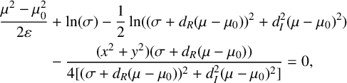 $$ \begin{align} \frac{\mu^2 -\mu_0^2}{2\varepsilon} &+ \ln(\sigma) - \frac{1}{2}\ln ((\sigma+d_R(\mu-\mu_0))^2 + d_I^2(\mu-\mu_0)^2) \nonumber \\ &- \frac{(x^2+y^2)(\sigma + d_R(\mu-\mu_0))}{4[(\sigma+d_R(\mu-\mu_0))^2 + d_I^2 (\mu-\mu_0)^2]} = 0, \end{align} $$
where we recall that $d=d_R + i d_I$
in (2.1). Hence, to leading order asymptotically, we find that the spatio-temporal memory surface is parabolic in x and y,
$d=d_R + i d_I$
in (2.1). Hence, to leading order asymptotically, we find that the spatio-temporal memory surface is parabolic in x and y,
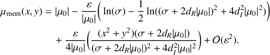 $$ \begin{align} \mu_{\mathrm{mem}}(x,y) &= \vert \mu_0 \vert - \frac{\varepsilon}{\vert \mu_0\vert} \bigg( \ln(\sigma) - \frac{1}{2}\ln ( (\sigma+2d_R\vert\mu_0\vert)^2 + 4d_I^2\vert\mu_0\vert^2) \bigg) \nonumber \\ &\quad + \frac{\varepsilon}{4\vert \mu_0 \vert} \bigg( \frac{(x^2+y^2)(\sigma + 2d_R\vert\mu_0\vert)}{(\sigma+2d_R\vert\mu_0\vert)^2 + 4d_I^2 \vert\mu_0\vert^2} \bigg) + \mathcal{O}(\varepsilon^2). \end{align} $$
For periodic initial data $A_0(x,y)=\cos (\pi(x-y)/L) \cos (\pi(x+y)/L)$
, the homogeneous solution for
$A_0(x,y)=\cos (\pi(x-y)/L) \cos (\pi(x+y)/L)$
, the homogeneous solution for $\mu> \mu _0$
is
$\mu> \mu _0$
is
 $$ \begin{align} A_h(x,y,\mu) = e^{(\mu^2-\mu_0^2 +2i\omega_0(\mu-\mu_0))/{2\varepsilon}} e^{-{4\pi^2 d (\mu-\mu_0)}/{L^2}} \cos \frac{\pi}{L}(x-y)\cos\frac{\pi}{L}(x+y). \end{align} $$
Hence, at any point $(x,y)$
, the real part of the argument vanishes for
$(x,y)$
, the real part of the argument vanishes for
 $$ \begin{align} \frac{1}{2\varepsilon}(\mu^2 - \mu_0^2) - \frac{4\pi^2 d (\mu - \mu_0)}{L^2} + \ln \bigg\lvert\! \cos\frac{\pi}{L}(x-y)\cos\frac{\pi}{L}(x+y)\bigg\rvert = 0. \end{align} $$
Asymptotically to leading order, one finds logarithmic dependence on $A_0$
,
$A_0$
,
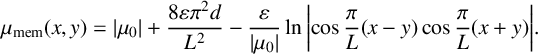 $$ \begin{align} \mu_{\mathrm{mem}}(x,y) = \vert \mu_0 \vert + \frac{8 \varepsilon \pi^2 d}{L^2} -\frac{\varepsilon}{\vert \mu_0\vert} \ln \bigg\lvert\! \cos\frac{\pi}{L}(x-y)\cos\frac{\pi}{L}(x+y)\bigg\rvert. \end{align} $$
These theoretical results for $\mu _{\mathrm {mem}}(x,y)$
with constant, Gaussian and periodic initial data are compared with simulations of (2.1) in Section 4.
$\mu _{\mathrm {mem}}(x,y)$
with constant, Gaussian and periodic initial data are compared with simulations of (2.1) in Section 4.
Remark 1 In [Reference Goh, Kaper and Vo17], for the CGL PDE in one dimension, we used the label homogeneous exit time curve. (There, homogeneous referred to the curve being defined by $A_h$
, not that the curve is spatially homogeneous.) Here, we label it instead the spatio-temporal memory surface, since it is determined by the memory of the initial data. One could also label it the spatio-temporal way-in way-out surface, in analogy with the way-in way-out function defined for DHB in analytic ODEs [Reference Neishtadt35, Reference Neishtadt36].
$A_h$
, not that the curve is spatially homogeneous.) Here, we label it instead the spatio-temporal memory surface, since it is determined by the memory of the initial data. One could also label it the spatio-temporal way-in way-out surface, in analogy with the way-in way-out function defined for DHB in analytic ODEs [Reference Neishtadt35, Reference Neishtadt36].
3.2. The spatio-temporal buffer surface
In this section, we focus on the particular solution $A_p(x,y,\mu )$
with special emphasis on the fourth (last) term in the general formula (2.5). We consider
$A_p(x,y,\mu )$
with special emphasis on the fourth (last) term in the general formula (2.5). We consider $\delta \le \mu \le \omega _0$
and label this term G, where
$\delta \le \mu \le \omega _0$
and label this term G, where
 $$ \begin{align} G(x,y,\mu) = ( \sqrt{2\pi} g(x,y,\mu+i\omega_0) +\mathcal{O}(\sqrt{\varepsilon})) e^{(\mu+i\omega_0)^2/{2\varepsilon}}. \end{align} $$
The function G is the component of the particular solution $A_p(x,y,\mu )$
that measures the deviation from the repelling QSS (where we recall that the first three terms in (2.5) represent the QSS). It is generated by passage over the saddle point at
$A_p(x,y,\mu )$
that measures the deviation from the repelling QSS (where we recall that the first three terms in (2.5) represent the QSS). It is generated by passage over the saddle point at $\mu =-i\omega _0$
in the complex
$\mu =-i\omega _0$
in the complex $\mu $
-plane, as shown in Appendix A. It is present in all solutions that start from initial data at any
$\mu $
-plane, as shown in Appendix A. It is present in all solutions that start from initial data at any $\mu _0<0$
, including solutions on the attracting QSS.
$\mu _0<0$
, including solutions on the attracting QSS.
The spatio-temporal buffer surface is defined as the surface along which
 $$ \begin{align} \lvert G(x,y,\mu) \rvert = 1, \end{align} $$
to leading order. Here, we derive a general formula for the spatio-temporal buffer surface for smooth, bounded sources $I_a(x,y)$
, and asymptotic formulas for it with constant, Gaussian, periodic and stripe sources. We see that, in general, G ceases to be exponentially small and becomes
$I_a(x,y)$
, and asymptotic formulas for it with constant, Gaussian, periodic and stripe sources. We see that, in general, G ceases to be exponentially small and becomes $\mathcal {O}(1)$
in a spatially dependent manner. This implies that all solutions with initial data given at
$\mathcal {O}(1)$
in a spatially dependent manner. This implies that all solutions with initial data given at $\mu _0<0$
, including those on the attracting QSS, must leave an
$\mu _0<0$
, including those on the attracting QSS, must leave an $\mathcal {O}(1)$
neighbourhood of the repelling QSS when
$\mathcal {O}(1)$
neighbourhood of the repelling QSS when $\mu $
reaches the buffer surface, irrespective of how large
$\mu $
reaches the buffer surface, irrespective of how large $|\mu _0|$
is; that is, irrespective of how far in the distant past the solutions approached the attracting QSS.
$|\mu _0|$
is; that is, irrespective of how far in the distant past the solutions approached the attracting QSS.
From (3.9), we find that the spatio-temporal buffer surface is given implicitly by
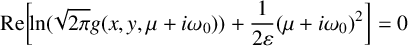 $$ \begin{align*} \mathrm{Re} \bigg[\!\!\ln ( \sqrt{2\pi} g(x,y,\mu+i\omega_0)) + \frac{1}{2\varepsilon} (\mu+i\omega_0)^2 \bigg] = 0 \end{align*} $$
for general smooth and bounded source terms $I_a(x,y)$
. We label the solution
$I_a(x,y)$
. We label the solution $\mu _{\mathrm {buf}}(x,y)$
. Its graph is the spatio-temporal buffer surface. To leading order,
$\mu _{\mathrm {buf}}(x,y)$
. Its graph is the spatio-temporal buffer surface. To leading order,
 $$ \begin{align} \mu_{\mathrm{buf}}^2(x,y) = \omega_0^2 - \varepsilon \ln(2\pi) - 2\varepsilon \ln\lvert g(x,y,\omega_0+i \omega_0)\rvert. \end{align} $$
At each point $(x,y)$
, the buffer surface
$(x,y)$
, the buffer surface $\mu _{\mathrm {buf}}(x,y)$
determines the time at which the deviation of
$\mu _{\mathrm {buf}}(x,y)$
determines the time at which the deviation of $A_p(x,y,\mu )$
from the repelling QSS ceases to be exponentially small.
$A_p(x,y,\mu )$
from the repelling QSS ceases to be exponentially small.
We begin with constant source terms, $I_C(x,y)=c$
, and set
$I_C(x,y)=c$
, and set $c=1$
without loss of generality. Substituting this into the integral for g in (2.5), we find
$c=1$
without loss of generality. Substituting this into the integral for g in (2.5), we find
 $$ \begin{align} g(x,y,\mu-\tilde{\mu}) = 1\quad \textrm{for all } (x,y) \quad \textrm{and}\quad \mu>\tilde{\mu} \ge \mu_0. \end{align} $$
Hence, by (3.11), the buffer surface is to leading order
 $$ \begin{align} \mu_{\mathrm{buf}}(x,y) = \omega_0 - \frac{\varepsilon}{2\omega_0} \ln(2\pi)\quad \textrm{for all } (x,y). \end{align} $$
It is independent of $(x,y)$
. Hence, at all points in the domain, the particular solution ceases to be exponentially small uniformly at this time,
$(x,y)$
. Hence, at all points in the domain, the particular solution ceases to be exponentially small uniformly at this time, $\mu _{\mathrm {buf}}$
.
$\mu _{\mathrm {buf}}$
.
Next, we consider Gaussian source terms, $I_G(x,y)=e^{{-(x^2+y^2)}/{4\sigma }}$
with
$I_G(x,y)=e^{{-(x^2+y^2)}/{4\sigma }}$
with $\sigma>0$
. Using (2.5), we find
$\sigma>0$
. Using (2.5), we find
 $$ \begin{align*} g(x,y,\mu-\tilde{\mu}) = \bigg( \frac{\sigma}{\sigma+d(\mu-\tilde{\mu})} \bigg) \,\mathrm{exp} \bigg[ \frac{-(x^2+y^2)}{4(\sigma+ d(\mu-\tilde{\mu}))}\bigg]. \end{align*} $$
Hence, (3.11) implies that, to leading order, the buffer surface is
 $$ \begin{align} \mu_{\mathrm{buf}}(x,y) &= \omega_0 - \frac{\varepsilon}{2\omega_0} \ln \bigg(\frac{2\pi\sigma^2}{(\sigma+\omega_0(d_R-d_I))^2 + \omega_0^2 (d_R+d_I)^2}\bigg) \nonumber \\ &\quad + \frac{\varepsilon}{4\omega_0} \bigg[\frac{(\sigma+\omega_0(d_R-d_I))}{(\sigma+\omega_0(d_R-d_I))^2 + \omega_0^2 (d_R+d_I)^2}\bigg] (x^2+y^2). \end{align} $$
For periodic source terms, $I_P(x,y)=\cos (\pi(x-y)/L) \cos (\pi(x+y)/L)$
, (2.5) yields
$I_P(x,y)=\cos (\pi(x-y)/L) \cos (\pi(x+y)/L)$
, (2.5) yields
 $$ \begin{align*} g(x,y,\mu-\tilde{\mu}) = e^{-4\pi^2 d(\mu -\tilde{\mu})/L^2} \cos\frac{\pi}{L}(x-y)\cos\frac{\pi}{L}(x+y). \end{align*} $$
Hence, (3.11) implies that, to leading order, the buffer surface is
 $$ \begin{align} \mu_{\mathrm{buf}}(x,y) &= \omega_0 -\frac{\varepsilon}{2\omega_0}\ln(2\pi) +\frac{4\varepsilon\pi^2(d_R - d_I)}{L^2} \nonumber \\ &\quad -\frac{\varepsilon}{\omega_0} \ln\bigg\lvert\!\cos\frac{\pi}{L}(x-y) \cos\frac{\pi}{L}(x+y)\bigg\rvert. \end{align} $$
Finally, we let H denote the Heaviside step function ( $1$
on
$1$
on $x>0$
and
$x>0$
and $0$
on
$0$
on $x<0$
) and study stripe source terms
$x<0$
) and study stripe source terms
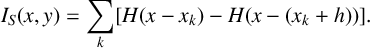 $$ \begin{align*} I_S(x,y)=\sum_k [ H(x-x_k)-H(x-(x_k+h)) ]. \end{align*} $$
Here, h is the width of the stripe, $x_k$
denotes the left edge of the kth stripe and
$x_k$
denotes the left edge of the kth stripe and $x_{k+1}-x_k =\Delta> h$
for each k. We use (2.5) to derive
$x_{k+1}-x_k =\Delta> h$
for each k. We use (2.5) to derive
 $$ \begin{align} g(x,y,\mu-\tilde{\mu}) = \frac{1}{2} \sum_{k} \bigg( \operatorname{erf} \bigg( \frac{x_k+h-x}{\sqrt{4d(\mu-\tilde{\mu})}} \bigg) - \operatorname{erf} \bigg( \frac{x_k-x}{\sqrt{4d(\mu-\tilde{\mu})}} \bigg) \bigg), \end{align} $$
where $\operatorname {erf}z = {2}/{\sqrt {\pi }} \int _0^z e^{-t^2}\,dt$
is the error function. Hence, (3.11) implies that, to leading order, the buffer surface is given by
$\operatorname {erf}z = {2}/{\sqrt {\pi }} \int _0^z e^{-t^2}\,dt$
is the error function. Hence, (3.11) implies that, to leading order, the buffer surface is given by
 $$ \begin{align} \mu_{\mathrm{buf}}(x,y) = \omega_0 - \frac{\varepsilon}{2\omega_0} \ln(2\pi) - \frac{\varepsilon}{\omega_0} \ln \lvert g(x,y,\omega_0(1+i)) \rvert, \end{align} $$
where g is given by (3.16). For these source terms, the spatio-temporal buffer surface is compared with the numerical solutions of the PDE (2.1) in Section 4.
4. DHB in the CGL equation with constant, Gaussian and stripe sources
In this section, we report on the spatially dependent duration of the DHB observed in direct numerical simulations of solutions of the CGL PDE (2.1) with $\mu _0<0$
. We examine both cases in which the initial time satisfies
$\mu _0<0$
. We examine both cases in which the initial time satisfies $\mu _0 \in (-\omega _0,0)$
and
$\mu _0 \in (-\omega _0,0)$
and $\mu _0 \le -\omega _0$
. We recall that the escape surface is the graph of the time
$\mu _0 \le -\omega _0$
. We recall that the escape surface is the graph of the time $\mu _{\mathrm {esc}}(x,y)$
in
$\mu _{\mathrm {esc}}(x,y)$
in $(x,y,\mu )$
space. Numerically, we obtain
$(x,y,\mu )$
space. Numerically, we obtain $\mu _{\mathrm {esc}}(x,y)$
by calculating the set of points at which
$\mu _{\mathrm {esc}}(x,y)$
by calculating the set of points at which $\lvert \mathrm { Re}(A_{\mathrm {num}}(x,y)) - \mathrm {Re}(A_{\mathrm {QSS}}(x,y)) \rvert = \delta _{\mathrm {th}}$
, where
$\lvert \mathrm { Re}(A_{\mathrm {num}}(x,y)) - \mathrm {Re}(A_{\mathrm {QSS}}(x,y)) \rvert = \delta _{\mathrm {th}}$
, where $A_{\mathrm {num}}(x,y)$
is the numerically computed solution of (2.1),
$A_{\mathrm {num}}(x,y)$
is the numerically computed solution of (2.1), $A_{\mathrm { QSS}}(x,y)$
is the value of A along the QSS (2.2) and
$A_{\mathrm { QSS}}(x,y)$
is the value of A along the QSS (2.2) and $\delta _{\mathrm {th}}$
denotes a threshold.
$\delta _{\mathrm {th}}$
denotes a threshold.
We show that $\mu _{\mathrm {esc}}(x,y)$
agrees with the predictions made from the memory and buffer surfaces. At each point
$\mu _{\mathrm {esc}}(x,y)$
agrees with the predictions made from the memory and buffer surfaces. At each point $(x,y)$
,
$(x,y)$
,
 $$ \begin{align*} \mu_{\mathrm{esc}}(x,y) \approx {\min}(\mu_{\mathrm{mem}}(x,y),\mu_{\mathrm{buf}}(x,y)). \end{align*} $$
We work with several different types of source terms (constant, Gaussian and stripe) and with the asymptotic expansions for these surfaces derived in Section 3.
In the numerical simulations, we used symmetric Strang splitting [Reference MacNamara, Strang, Glowinski, Osher and Yin33], with centred finite differences for the spatial discretization and fourth-order Runge–Kutta with fixed time step for the time discretization. The results were also checked independently using a Chebyshev grid for the spatial discretization, finding good agreement.
4.1. DHB with constant source term
In the first representative simulation, we study DHB in (2.1) with constant source term $I_C(x,y)=1$
and Gaussian initial data
$I_C(x,y)=1$
and Gaussian initial data
 $$ \begin{align} A_0(x,y) = c_1+c_2 e^{-(x^2+y^2)/4\sigma},\quad c_1,\quad c_2> 0, \end{align} $$
given at $\mu _0=-0.3$
, which we note is in
$\mu _0=-0.3$
, which we note is in $(-\omega _0,0)$
. The dynamics are shown in Figure 1, and a quantitative comparison between the escape surface for this solution and the memory surface calculated using the analysis of the previous section is shown in Figure 2. (Note that the solution is radially symmetric, because the initial data was chosen to be radially symmetric for simplicity in this first simulation; see also Figure 1(a).)
$(-\omega _0,0)$
. The dynamics are shown in Figure 1, and a quantitative comparison between the escape surface for this solution and the memory surface calculated using the analysis of the previous section is shown in Figure 2. (Note that the solution is radially symmetric, because the initial data was chosen to be radially symmetric for simplicity in this first simulation; see also Figure 1(a).)
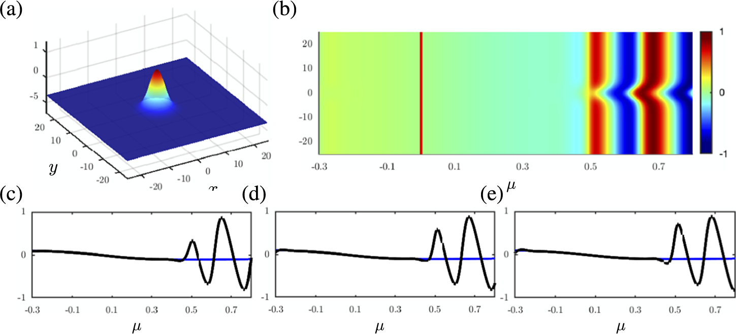
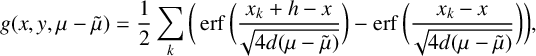
Figure 1 Delayed onset of oscillations in (2.1) with constant source term $I_C(x,y)=1$
and Gaussian initial data (4.1) given at
$I_C(x,y)=1$
and Gaussian initial data (4.1) given at $\mu _0 = -0.3$
. (a) Snapshot of
$\mu _0 = -0.3$
. (a) Snapshot of $\operatorname {Re}u$
at
$\operatorname {Re}u$
at $\mu = -\mu _0 = 0.3$
showing that the solution is radially symmetric. (b) Space-time evolution along
$\mu = -\mu _0 = 0.3$
showing that the solution is radially symmetric. (b) Space-time evolution along $y=0$
. The red line indicates the instantaneous Hopf bifurcation. The temporal evolution of
$y=0$
. The red line indicates the instantaneous Hopf bifurcation. The temporal evolution of $\operatorname {Re}u$
(black curve) is compared with the QSS (blue curve) at the centre of the Gaussian at
$\operatorname {Re}u$
(black curve) is compared with the QSS (blue curve) at the centre of the Gaussian at $(x,y)=(0,0)$
(c), at a radial distance of three spatial units from the origin at
$(x,y)=(0,0)$
(c), at a radial distance of three spatial units from the origin at $(x,y) = ({3}/{\sqrt {2}},{3}/{\sqrt {2}})$
(d), and at a radial distance of 10 spatial units from the origin at
$(x,y) = ({3}/{\sqrt {2}},{3}/{\sqrt {2}})$
(d), and at a radial distance of 10 spatial units from the origin at $(x,y) = ({10}/{\sqrt {2}},{10}/{\sqrt {2}})$
(e). In each case, the numerical solution stays close to the QSS well past the instantaneous Hopf bifurcation at
$(x,y) = ({10}/{\sqrt {2}},{10}/{\sqrt {2}})$
(e). In each case, the numerical solution stays close to the QSS well past the instantaneous Hopf bifurcation at $\mu = 0$
, after which there is a hard onset to large-amplitude oscillations.
$\mu = 0$
, after which there is a hard onset to large-amplitude oscillations.
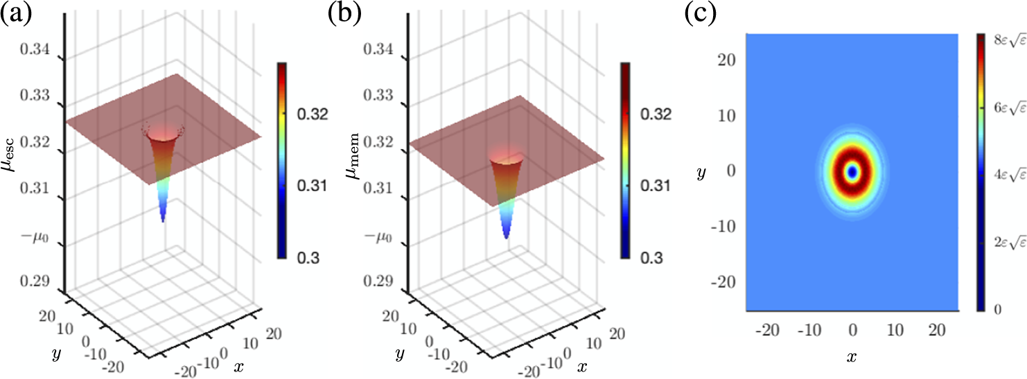
Figure 2 (a) In the three-dimensional $(x,y,\mu )$
space, the surface
$(x,y,\mu )$
space, the surface $\mu _{\mathrm {esc}}(x,y)$
is where the hard onset of the oscillations occurs. It has been obtained from direct numerical simulation of the PDE (2.1) with constant source term
$\mu _{\mathrm {esc}}(x,y)$
is where the hard onset of the oscillations occurs. It has been obtained from direct numerical simulation of the PDE (2.1) with constant source term $I_C(x,y)=1$
and Gaussian initial data
$I_C(x,y)=1$
and Gaussian initial data $A_0(x,y)=c_1+c_2 e^{{-(x^2+ y^2)}/{4\sigma }}$
with
$A_0(x,y)=c_1+c_2 e^{{-(x^2+ y^2)}/{4\sigma }}$
with $(c_1,c_2,\sigma ) = (0.5,0.5,2.5)$
, given at
$(c_1,c_2,\sigma ) = (0.5,0.5,2.5)$
, given at $\mu _0=-0.3$
. (b) The memory surface
$\mu _0=-0.3$
. (b) The memory surface $\mu _{\mathrm {mem}}(x,y)$
is given by (3.4). It gives the leading order asymptotics of the escape time for all
$\mu _{\mathrm {mem}}(x,y)$
is given by (3.4). It gives the leading order asymptotics of the escape time for all $(x,y)$
. (c) The difference
$(x,y)$
. (c) The difference $|\mu _{\mathrm {esc}} (x,y) - \mu _{\mathrm {mem}}(x,y)|$
is shown in the projection onto the
$|\mu _{\mathrm {esc}} (x,y) - \mu _{\mathrm {mem}}(x,y)|$
is shown in the projection onto the $(x,y)$
plane. Here, the parameters are
$(x,y)$
plane. Here, the parameters are $d=1$
,
$d=1$
, $\omega _0=0.5$
,
$\omega _0=0.5$
, $\alpha =0.2$
and
$\alpha =0.2$
and $\varepsilon =0.01$
.
$\varepsilon =0.01$
.
As expected, the solution stays near the repelling QSS at least until $\mu $
reaches
$\mu $
reaches $-\mu _0$
(see Figure 1(a) and (b)). Then, the delayed, post-Hopf, temporal oscillations are initiated at the origin of the domain, near
$-\mu _0$
(see Figure 1(a) and (b)). Then, the delayed, post-Hopf, temporal oscillations are initiated at the origin of the domain, near $\mu =-\mu _0$
(see Figure 1(c)). As
$\mu =-\mu _0$
(see Figure 1(c)). As $\mu $
continues to slowly increase, the oscillations occur on successively larger disks about the origin (see Figure 1(d) and (e) for two other points). Then, once
$\mu $
continues to slowly increase, the oscillations occur on successively larger disks about the origin (see Figure 1(d) and (e) for two other points). Then, once $\mu $
reaches approximately
$\mu $
reaches approximately $0.327$
(which depends on the chosen threshold), there is a fairly rapid transition to large-scale oscillations, and these occur on the entire domain.
$0.327$
(which depends on the chosen threshold), there is a fairly rapid transition to large-scale oscillations, and these occur on the entire domain.
For this first simulation, we also show the escape surface in Figure 2(a). Below the escape surface, that is for all $\mathcal {O}(1)$
values
$\mathcal {O}(1)$
values $\mu < \mu _{\mathrm {esc}}(x,y)$
, the solution is near the repelling QSS. Then, at each point
$\mu < \mu _{\mathrm {esc}}(x,y)$
, the solution is near the repelling QSS. Then, at each point $(x,y)$
, the oscillations of amplitude
$(x,y)$
, the oscillations of amplitude $\mathcal {O}(\sqrt {\varepsilon })$
set in when
$\mathcal {O}(\sqrt {\varepsilon })$
set in when $\mu $
reaches
$\mu $
reaches $\mu _{\mathrm {esc}}(x,y)$
. Furthermore, at each point
$\mu _{\mathrm {esc}}(x,y)$
. Furthermore, at each point $(x,y)$
, the amplitude of the oscillations becomes large (
$(x,y)$
, the amplitude of the oscillations becomes large ( $\mathcal {O}(1)$
) as soon as
$\mathcal {O}(1)$
) as soon as $\mu $
is slightly beyond
$\mu $
is slightly beyond $\mu _{\mathrm {esc}}(x,y)$
, which confirms for all points
$\mu _{\mathrm {esc}}(x,y)$
, which confirms for all points $(x,y)$
what is shown for just three points in Figure 1.
$(x,y)$
what is shown for just three points in Figure 1.
For comparison, we show the memory surface $\mu _{\mathrm {mem}} (x,y)$
in Figure 2(b). The memory surface was computed as follows. First, we combined the homogeneous solutions (3.1) and (3.3) to determine the homogeneous solution,
$\mu _{\mathrm {mem}} (x,y)$
in Figure 2(b). The memory surface was computed as follows. First, we combined the homogeneous solutions (3.1) and (3.3) to determine the homogeneous solution, $A_h$
, with the initial data (4.1),
$A_h$
, with the initial data (4.1), $A_0(x,y)=c_1+c_2 e^{{-(x^2+ y^2)}/{4\sigma }}$
. Then, by enforcing the condition
$A_0(x,y)=c_1+c_2 e^{{-(x^2+ y^2)}/{4\sigma }}$
. Then, by enforcing the condition $| A_h | = 1$
, we obtained the leading order asymptotic relationship
$| A_h | = 1$
, we obtained the leading order asymptotic relationship
 $$ \begin{align} \mu^2 - \mu_0^2 + 2\varepsilon \ln \bigg| c_1 + c_2 \frac{\sigma}{\sigma+d(\mu-\mu_0)} \exp \bigg( \frac{-(x^2+y^2)}{4(\sigma+d(\mu-\mu_0))} \bigg) \bigg| = 0 \end{align} $$
for the memory surface corresponding to this $A_0$
.
$A_0$
.
The difference $|\mu _{\mathrm {esc}} (x,y) - \mu _{\mathrm {mem}}(x,y)|$
is shown in Figure 2(c). At the centre of the Gaussian, the difference is small (with magnitude of approximately
$|\mu _{\mathrm {esc}} (x,y) - \mu _{\mathrm {mem}}(x,y)|$
is shown in Figure 2(c). At the centre of the Gaussian, the difference is small (with magnitude of approximately $10^{-5}$
, that is,
$10^{-5}$
, that is, $\mathcal {O}(\varepsilon ^{5/2})$
). Then, in an annular region about the origin (red and dark red), the difference is slightly larger, due to nonlinear effects. Finally, both surfaces exhibit a fairly rapid transition into the regime (blue region in Figure 2(c), red in (a) and (b)) where they are essentially constant, since the Gaussian is tiny. Here,
$\mathcal {O}(\varepsilon ^{5/2})$
). Then, in an annular region about the origin (red and dark red), the difference is slightly larger, due to nonlinear effects. Finally, both surfaces exhibit a fairly rapid transition into the regime (blue region in Figure 2(c), red in (a) and (b)) where they are essentially constant, since the Gaussian is tiny. Here, $\mu _{\mathrm {mem}}(x,y)=\sqrt {\mu _0^2 - 2 \varepsilon \ln c_1} \approx 0.322$
to leading order (as obtained from (4.2) for large
$\mu _{\mathrm {mem}}(x,y)=\sqrt {\mu _0^2 - 2 \varepsilon \ln c_1} \approx 0.322$
to leading order (as obtained from (4.2) for large $x^2 + y^2$
), which agrees well with the value observed numerically in (2.1). Similar results were observed for solutions and the escape and memory surfaces with other values of
$x^2 + y^2$
), which agrees well with the value observed numerically in (2.1). Similar results were observed for solutions and the escape and memory surfaces with other values of $-\omega _0< \mu _0<0$
(data not shown).
$-\omega _0< \mu _0<0$
(data not shown).
Moreover, for the CGL with this (constant) source term, the buffer surface lies above the memory surface for all $(x,y)$
in three dimensions, since
$(x,y)$
in three dimensions, since ${\mu _{\mathrm {buf}}(x,y) = \sqrt {\omega _0^2 - \varepsilon \ln (2\pi )}\!\approx \!0.481}$
for all
${\mu _{\mathrm {buf}}(x,y) = \sqrt {\omega _0^2 - \varepsilon \ln (2\pi )}\!\approx \!0.481}$
for all $(x,y)$
. Hence, for all
$(x,y)$
. Hence, for all $(x,y)$
, the minimum in
$(x,y)$
, the minimum in $\mu _{\mathrm {esc}}(x,y) \sim \mathrm {\min } \{ \mu _{\mathrm {mem}} (x,y), \mu _{\mathrm {buf}}(x,y) \}$
is given entirely by the memory surface in this simulation.
$\mu _{\mathrm {esc}}(x,y) \sim \mathrm {\min } \{ \mu _{\mathrm {mem}} (x,y), \mu _{\mathrm {buf}}(x,y) \}$
is given entirely by the memory surface in this simulation.
The second representative simulation is also with $I_C(x,y)=1$
. However, now the initial data given at
$I_C(x,y)=1$
. However, now the initial data given at $-\omega _0 < \mu _0 < 0$
is periodic,
$-\omega _0 < \mu _0 < 0$
is periodic,
 $$ \begin{align*} A_0(x,y) = p_1 + p_2 \cos \frac{\pi}{L}(x-y) \cos \frac{\pi}{L}(x+y), \end{align*} $$
with $p_1>p_2>0$
, so that
$p_1>p_2>0$
, so that $A_0(x,y)$
is strictly positive everywhere. The results are shown in Figure 3.
$A_0(x,y)$
is strictly positive everywhere. The results are shown in Figure 3.

Figure 3 (a) In the three-dimensional $(x,y,\mu )$
space, the surface
$(x,y,\mu )$
space, the surface $\mu _{\mathrm {esc}}(x,y)$
is where the hard onset of the oscillations occurs. It has been obtained from direct simulation of (2.1) with constant source term
$\mu _{\mathrm {esc}}(x,y)$
is where the hard onset of the oscillations occurs. It has been obtained from direct simulation of (2.1) with constant source term $I_C(x,y)=1$
and periodic initial data
$I_C(x,y)=1$
and periodic initial data $A_0(x,y)=p_1+p_2 \cos (\pi(x-y)/L) \cos (\pi(x+y)/L)$
at
$A_0(x,y)=p_1+p_2 \cos (\pi(x-y)/L) \cos (\pi(x+y)/L)$
at $\mu _0=-0.3$
with
$\mu _0=-0.3$
with $(p_1,p_2,L)=(1,0.5,25)$
. (b) The memory surface
$(p_1,p_2,L)=(1,0.5,25)$
. (b) The memory surface $\mu _{\mathrm {mem}}(x,y)$
given by (3.7). (c) The surface
$\mu _{\mathrm {mem}}(x,y)$
given by (3.7). (c) The surface $|\mu _{\mathrm {num}} (x,y) - \mu _{\mathrm {mem}}(x,y)|$
shown in the projection onto the
$|\mu _{\mathrm {num}} (x,y) - \mu _{\mathrm {mem}}(x,y)|$
shown in the projection onto the $(x,y)$
plane. The parameters are
$(x,y)$
plane. The parameters are $d=1, \omega _0=0.5$
,
$d=1, \omega _0=0.5$
, $\alpha = 0.2$
and
$\alpha = 0.2$
and $\varepsilon =0.01$
.
$\varepsilon =0.01$
.
The escape surface computed from the numerical simulations (Figure 3(a)) shows that the oscillations first occur at time $\mu \approx 0.281$
at the points
$\mu \approx 0.281$
at the points $(x,y)=(j_1 L, j_2 L)$
, where
$(x,y)=(j_1 L, j_2 L)$
, where $j_1,j_2=-1,0,1$
(dark blue), that is, at the maxima of
$j_1,j_2=-1,0,1$
(dark blue), that is, at the maxima of $A_0(x,y)$
, where
$A_0(x,y)$
, where $\cos (\pi(x-y)/L) \cos (\pi(x+y)/L)=1$
. About each of those points, the oscillations set in on successively larger disks as
$\cos (\pi(x-y)/L) \cos (\pi(x+y)/L)=1$
. About each of those points, the oscillations set in on successively larger disks as $\mu $
slowly increases, until those disks collide at
$\mu $
slowly increases, until those disks collide at $\mu \approx 0.306$
(near the transition from yellow to orange). Then, as
$\mu \approx 0.306$
(near the transition from yellow to orange). Then, as $\mu $
increases further, the escape surface consists of the four inverted paraboloid segments (orange and red). The peaks occur at time
$\mu $
increases further, the escape surface consists of the four inverted paraboloid segments (orange and red). The peaks occur at time $\mu \approx 0.315$
at the points
$\mu \approx 0.315$
at the points $(x,y)=( {j_1 L}/{2}, {j_2 L}/{2})$
, where
$(x,y)=( {j_1 L}/{2}, {j_2 L}/{2})$
, where $j_1,j_2=-1,1$
(dark red), that is, at the minima of
$j_1,j_2=-1,1$
(dark red), that is, at the minima of $A_0(x,y)$
, where
$A_0(x,y)$
, where $\cos (\pi(x-y)/L) \cos (\pi(x+y)/L) = -1$
.
$\cos (\pi(x-y)/L) \cos (\pi(x+y)/L) = -1$
.
For comparison, the memory surface $\mu _{\mathrm {mem}}(x,y)$
is defined by
$\mu _{\mathrm {mem}}(x,y)$
is defined by
 $$ \begin{align} \mu^2-\mu_0^2 + 2\varepsilon \ln \bigg| p_1+p_2 \exp \bigg(-\frac{4\pi^2 d(\mu-\mu_0)}{L^2} \bigg) \cos \frac{\pi}{L}(x-y) \cos \frac{\pi}{L}(x+y) \bigg| = 0, \end{align} $$
and shown in Figure 3(b). It has global minima (dark blue) when
 $$ \begin{align*}\mu_{\mathrm{mem}}=\sqrt{\lvert \mu_0 \rvert^2 - 2 \varepsilon \ln ( 1 + 0.5 e^{({-8\pi^2 d |\mu_0|})/{L^2}} ) } \approx 0.2866 \end{align*} $$
to leading order, with $\mu _0=-0.3$
. These occur at the points where
$\mu _0=-0.3$
. These occur at the points where $A_0(x,y)$
has its maxima. Also, the memory surface has global maxima (dark red) when
$A_0(x,y)$
has its maxima. Also, the memory surface has global maxima (dark red) when $\mu \approx 0.3211$
, at the points where
$\mu \approx 0.3211$
, at the points where $A_0(x,y)$
has its minima. In between, it has the same conical shape qualitatively as the escape surface.
$A_0(x,y)$
has its minima. In between, it has the same conical shape qualitatively as the escape surface.
The difference between $\mu _{\mathrm {esc}}(x,y)$
and
$\mu _{\mathrm {esc}}(x,y)$
and $\mu _{\mathrm {mem}}(x,y)$
is shown in Figure 3(c). The nonlinear terms cause
$\mu _{\mathrm {mem}}(x,y)$
is shown in Figure 3(c). The nonlinear terms cause $\mu _{\mathrm {esc}}$
to grow more steeply from the local minima, compared with the memory surface, so that the disks collide at a slightly later time than for the memory surface. Then, after the disks collide, the inverted paraboloids are slightly wider in
$\mu _{\mathrm {esc}}$
to grow more steeply from the local minima, compared with the memory surface, so that the disks collide at a slightly later time than for the memory surface. Then, after the disks collide, the inverted paraboloids are slightly wider in $\mu _{\mathrm {esc}}(x,y)$
due to the nonlinear terms.
$\mu _{\mathrm {esc}}(x,y)$
due to the nonlinear terms.
Finally, for this second representative simulation, we report that the buffer surface also lies above the memory surface for all $(x,y)$
in three dimensions. Indeed, with constant source
$(x,y)$
in three dimensions. Indeed, with constant source $I_C(x,y)=1$
,
$I_C(x,y)=1$
, $\mu _{\mathrm {buf}}(x,y) = \sqrt {\omega _0^2 - \varepsilon \ln (2\pi )}\approx 0.481$
. Hence, here also the minimum is given by the memory surface for all
$\mu _{\mathrm {buf}}(x,y) = \sqrt {\omega _0^2 - \varepsilon \ln (2\pi )}\approx 0.481$
. Hence, here also the minimum is given by the memory surface for all $(x,y)$
.
$(x,y)$
.
Remark 2 In the second simulation, we also combined two homogeneous solutions, (3.1) and (3.6), to determine the homogeneous solution $A_h$
that corresponds to the periodic initial profile
$A_h$
that corresponds to the periodic initial profile $A_0(x,y) = p_1 + p_2 \cos (\pi(x-y)/L) \cos (\pi(x+y)/L)$
. Then, by setting
$A_0(x,y) = p_1 + p_2 \cos (\pi(x-y)/L) \cos (\pi(x+y)/L)$
. Then, by setting $| A_h| = 1$
, we obtain (4.3).
$| A_h| = 1$
, we obtain (4.3).
Remark 3 We also explored the effect of giving the initial data at different times, including $\mu _0 < - \omega _0$
, while keeping the source term and initial data the same as in the second simulation. In these simulations (data not shown), we observe that
$\mu _0 < - \omega _0$
, while keeping the source term and initial data the same as in the second simulation. In these simulations (data not shown), we observe that $\mu _{\mathrm {esc}}(x,y) = \omega _0 - \varepsilon \ln (2\pi )$
to leading order for all
$\mu _{\mathrm {esc}}(x,y) = \omega _0 - \varepsilon \ln (2\pi )$
to leading order for all $(x,y)$
, as determined by
$(x,y)$
, as determined by $A_p$
(recall (3.13)). This is as expected from the analysis, because
$A_p$
(recall (3.13)). This is as expected from the analysis, because $\mu _{\mathbf {buf}}(x,y) < \mu _{\mathrm {mem}}(x,y)$
at all points when the initial data is given at time
$\mu _{\mathbf {buf}}(x,y) < \mu _{\mathrm {mem}}(x,y)$
at all points when the initial data is given at time $\mu _0 < -\omega _0$
and
$\mu _0 < -\omega _0$
and $\varepsilon $
is sufficiently small.
$\varepsilon $
is sufficiently small.
4.2. DHB with Gaussian source term
Gaussian source terms can be used to model spatially localized, radially symmetric inputs, such as a circular spot of visible light that shines on the reactor in a chemical pattern-forming experiment. A representative example of (2.1) with Gaussian source term is shown in Figure 4. Here, $I_G(x,y) = \exp ( -({x^2+y^2})/{4\sigma } )$
with
$I_G(x,y) = \exp ( -({x^2+y^2})/{4\sigma } )$
with $\sigma = 1$
, and the initial data at
$\sigma = 1$
, and the initial data at $\mu _0 = -0.75$
(which is chosen so that
$\mu _0 = -0.75$
(which is chosen so that $\mu _0 < - \omega _0$
) is
$\mu _0 < - \omega _0$
) is
 $$ \begin{align*} A_0(x,y) = \cos \frac{\pi}{L}(x-y)\cos \frac{\pi}{L} (x+y)\quad\text{with } L=25. \end{align*} $$
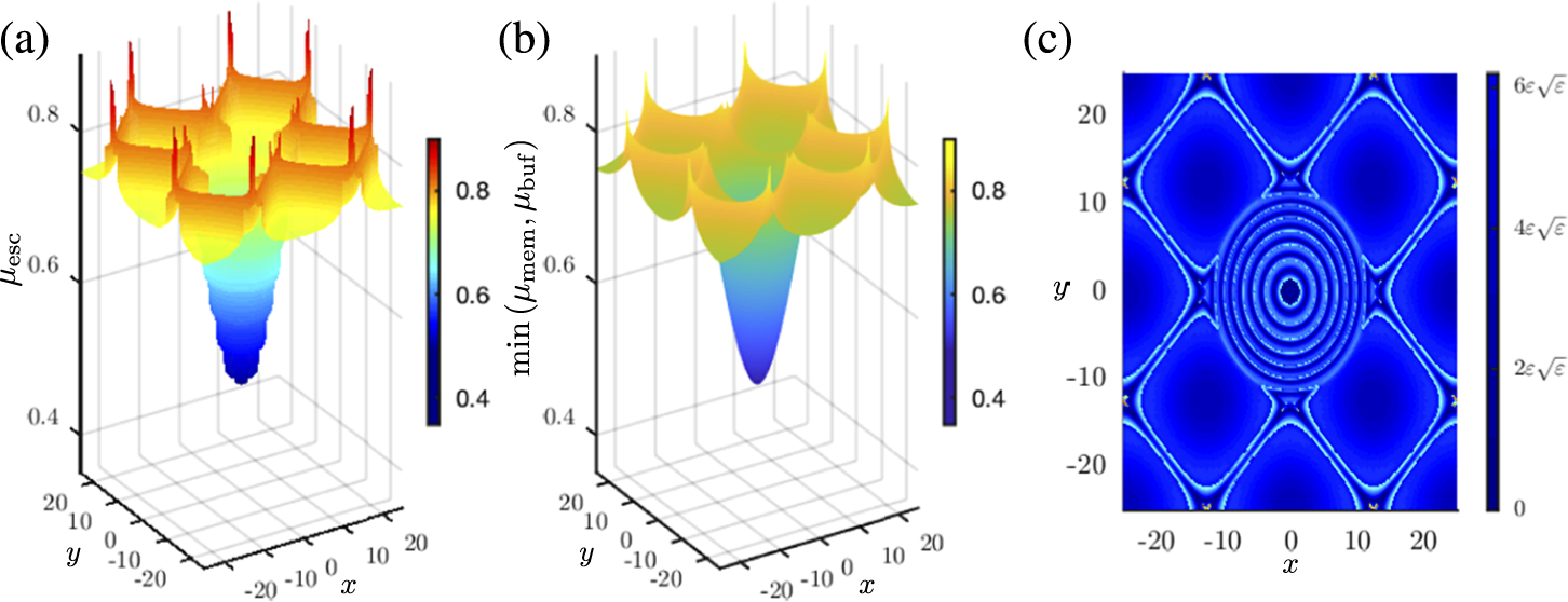
Figure 4 (a) In the three dimensional $(x,y,\mu )$
space, the surface
$(x,y,\mu )$
space, the surface $\mu _{\mathrm {esc}}(x,y)$
is where the hard onset of the oscillations occurs. It has been obtained from direct simulation of (2.1) with Gaussian source term
$\mu _{\mathrm {esc}}(x,y)$
is where the hard onset of the oscillations occurs. It has been obtained from direct simulation of (2.1) with Gaussian source term $I_G(x,y)=\exp ( -({x^2+y^2})/{4\sigma } )$
and periodic initial data
$I_G(x,y)=\exp ( -({x^2+y^2})/{4\sigma } )$
and periodic initial data $A_0(x,y)=\cos (\pi(x-y)/L) \cos (\pi(x+y)/L)$
at
$A_0(x,y)=\cos (\pi(x-y)/L) \cos (\pi(x+y)/L)$
at $\mu _0=-0.75$
with
$\mu _0=-0.75$
with $L=25$
. (b) The predicted escape surface is given by the minimum of
$L=25$
. (b) The predicted escape surface is given by the minimum of $\mu _{\mathrm {buf}}(x,y)$
(parabolic part) and
$\mu _{\mathrm {buf}}(x,y)$
(parabolic part) and $\mu _{\mathrm {mem}}(x,y)$
(periodic part). (c) The surface
$\mu _{\mathrm {mem}}(x,y)$
(periodic part). (c) The surface $|\mu _{\mathrm {esc}} (x,y) - \min \{ \mu _{\mathrm {mem}}, \mu _{\mathrm {buf}} \} |$
shown in the projection onto the
$|\mu _{\mathrm {esc}} (x,y) - \min \{ \mu _{\mathrm {mem}}, \mu _{\mathrm {buf}} \} |$
shown in the projection onto the $(x,y)$
plane. The parameters are
$(x,y)$
plane. The parameters are $d=1, \omega _0=0.5$
,
$d=1, \omega _0=0.5$
, $\alpha = 0.2$
and
$\alpha = 0.2$
and $\varepsilon =0.01$
.
$\varepsilon =0.01$
.
From direct numerical simulations of the PDE, we find that the domain of the escape surface (Figure 4(a)) can be split into two distinct parts: the annular region $R_G = \{(x,y) \mid x^2+y^2 \leq 11.5^2 \}$
and its complement
$R_G = \{(x,y) \mid x^2+y^2 \leq 11.5^2 \}$
and its complement $R_P = \mathbb {R}^2 \backslash R_G$
. On
$R_P = \mathbb {R}^2 \backslash R_G$
. On $R_G$
, the earliest numerically detected escape occurs at the origin for
$R_G$
, the earliest numerically detected escape occurs at the origin for $\mu \approx 0.4905$
. The escape surface is radially symmetric and increases on concentric rings, which thus creates a rotationally symmetric paraboloid. In contrast, for
$\mu \approx 0.4905$
. The escape surface is radially symmetric and increases on concentric rings, which thus creates a rotationally symmetric paraboloid. In contrast, for $(x,y)\in R_P$
, the escape surface is no longer radially symmetric, and is instead a periodic tile pattern, reflecting the initial data. The minima occur at
$(x,y)\in R_P$
, the escape surface is no longer radially symmetric, and is instead a periodic tile pattern, reflecting the initial data. The minima occur at $\mu \approx 0.738$
(yellow/green regions) and the maxima at
$\mu \approx 0.738$
(yellow/green regions) and the maxima at $\mu \approx 0.812$
(red lines between yellow/green regions).
$\mu \approx 0.812$
(red lines between yellow/green regions).
For this source term and initial condition, the buffer surface is given by (3.14) and the memory surface is given by (3.7). In Figure 4(b), we plot $\mathrm {\min } \{ \mu _{\mathrm {buf}}(x,y), \mu _{\mathrm {mem}}(x,y) \}$
. On
$\mathrm {\min } \{ \mu _{\mathrm {buf}}(x,y), \mu _{\mathrm {mem}}(x,y) \}$
. On $R_G$
, the minimum is given by the buffer surface, whereas it is given by the memory surface on
$R_G$
, the minimum is given by the buffer surface, whereas it is given by the memory surface on $R_P$
. The buffer surface predicts that the earliest onset occurs at the origin at
$R_P$
. The buffer surface predicts that the earliest onset occurs at the origin at $\mu \approx 0.4908$
. The values of
$\mu \approx 0.4908$
. The values of $\mu _{\mathrm {buf}}$
increase in a radially symmetric fashion until
$\mu _{\mathrm {buf}}$
increase in a radially symmetric fashion until ${\mu \approx -\mu _0 = 0.75}$
on the boundary of
${\mu \approx -\mu _0 = 0.75}$
on the boundary of $R_G$
. Then, for
$R_G$
. Then, for $(x,y)$
on
$(x,y)$
on $R_P$
, the memory surface predicts the onset. (Compare Figure 4(a) and (b).)
$R_P$
, the memory surface predicts the onset. (Compare Figure 4(a) and (b).)
The difference $\lvert \mu _{\mathrm {esc}}(x,y)- \mathrm {\min }\{ \mu _{\mathrm {buf}}(x,y), \mu _{\mathrm {mem}}(x,y) \} \rvert $
is small throughout, as shown in Figure 4(c). The difference is especially small (of the order of the neglected terms in the asymptotic expansion) near the onset at the origin, which is at the minimum of the buffer surface, and also near the local minima of the memory surface.
$\lvert \mu _{\mathrm {esc}}(x,y)- \mathrm {\min }\{ \mu _{\mathrm {buf}}(x,y), \mu _{\mathrm {mem}}(x,y) \} \rvert $
is small throughout, as shown in Figure 4(c). The difference is especially small (of the order of the neglected terms in the asymptotic expansion) near the onset at the origin, which is at the minimum of the buffer surface, and also near the local minima of the memory surface.
4.3. DHB with stripe source term
Stripe source terms are also of fundamental interest. For example, chemical reactions irradiated with constant intensity light filtered through stripe masks can produce complex patterns (see [Reference Berenstein, Dolnik, Zhabotinsky and Epstein7, Reference Gentili and Micheau16] and references within).
Here, we use a simple model for a strictly positive stripe source term,
 $$ \begin{align} I_S(x,y)=1+\frac{1}{2}\sum_{k=-2}^2 [ H(x-x_k)-H(x-x_k-h) ], \end{align} $$
where h is the stripe width, $x_k$
denotes the left edge of the kth stripe and
$x_k$
denotes the left edge of the kth stripe and $x_{k+1}-x_k =\Delta> h$
. We set
$x_{k+1}-x_k =\Delta> h$
. We set $x_0= -1.25$
,
$x_0= -1.25$
, $h=2.5$
and
$h=2.5$
and $\Delta =10$
.
$\Delta =10$
.
For the PDE (2.1), the surfaces $\mu _{\mathrm {esc}}(x,y)$
(calculated from direct numerical simulations) and
$\mu _{\mathrm {esc}}(x,y)$
(calculated from direct numerical simulations) and $\mu _{\mathrm {buf}}(x,y)$
(calculated from (3.12) and (3.16)) are shown in Figure 5(a) and (b), along with the difference in Figure 5(c). From the plot of
$\mu _{\mathrm {buf}}(x,y)$
(calculated from (3.12) and (3.16)) are shown in Figure 5(a) and (b), along with the difference in Figure 5(c). From the plot of $\mu _{\mathrm {esc}}(x,y)$
, we see that the hard onset of oscillations occurs first at the points where
$\mu _{\mathrm {esc}}(x,y)$
, we see that the hard onset of oscillations occurs first at the points where $I_S(x,y)$
has its maximum, that is, inside the stripes. See the green stripes in the plot of
$I_S(x,y)$
has its maximum, that is, inside the stripes. See the green stripes in the plot of $\mu _{\mathrm {esc}}(x,y)$
in Figure 5(a). The buffer curve
$\mu _{\mathrm {esc}}(x,y)$
in Figure 5(a). The buffer curve $\mu _{\mathrm {buf}}(x,y)$
also has local minima inside the stripes (blue stripes in Figure 5(b)), and these stripes have approximately the same width as those of the escape surface. The difference in the green and blue stripes is of
$\mu _{\mathrm {buf}}(x,y)$
also has local minima inside the stripes (blue stripes in Figure 5(b)), and these stripes have approximately the same width as those of the escape surface. The difference in the green and blue stripes is of $\mathcal {O}(\varepsilon \sqrt {\varepsilon })$
.
$\mathcal {O}(\varepsilon \sqrt {\varepsilon })$
.
In the complementary regions, the PDE simulations show that the duration of the DHB is longer. The escape surface lies just below $\omega _0$
, by about
$\omega _0$
, by about $2\varepsilon $
(see the yellow stripes in Figure 5(a)). In the complementary regions, the buffer surface transitions more gradually to its local maxima, which also occur at the local minima of the source term. Here, the difference is of
$2\varepsilon $
(see the yellow stripes in Figure 5(a)). In the complementary regions, the buffer surface transitions more gradually to its local maxima, which also occur at the local minima of the source term. Here, the difference is of $\mathcal {O}(\varepsilon \sqrt {\varepsilon })$
.
$\mathcal {O}(\varepsilon \sqrt {\varepsilon })$
.
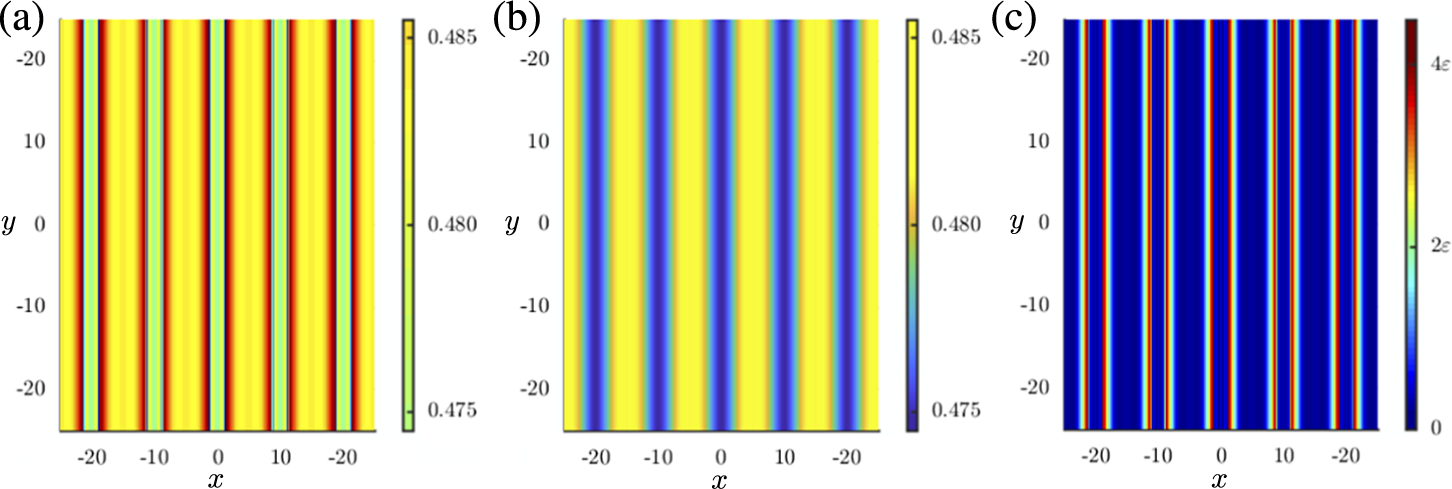
Figure 5 (a) The surface $\mu _{\mathrm {esc}}(x,y)$
, shown here in the projection onto the
$\mu _{\mathrm {esc}}(x,y)$
, shown here in the projection onto the $(x,y)$
plane, is where the hard onset of oscillations occurs. It has been obtained from numerical simulation of (2.1) with stripe source term
$(x,y)$
plane, is where the hard onset of oscillations occurs. It has been obtained from numerical simulation of (2.1) with stripe source term $I_S(x,y)$
(4.4) and constant initial data
$I_S(x,y)$
(4.4) and constant initial data $A_0(x,y)=1$
given at
$A_0(x,y)=1$
given at $\mu _0=-1$
. (b) The buffer surface
$\mu _0=-1$
. (b) The buffer surface $\mu _{\mathrm {buf}}(x,y)$
defined by (3.11), with g given by the linear combination of (3.12) and (3.16). (c) The difference
$\mu _{\mathrm {buf}}(x,y)$
defined by (3.11), with g given by the linear combination of (3.12) and (3.16). (c) The difference $|\mu _{\mathrm {esc}} (x,y) - \mu _{\mathrm {buf}}(x,y)|$
. The parameters are
$|\mu _{\mathrm {esc}} (x,y) - \mu _{\mathrm {buf}}(x,y)|$
. The parameters are $d = 1, \omega _0=0.5$
,
$d = 1, \omega _0=0.5$
, $\alpha = 0.2$
and
$\alpha = 0.2$
and $\varepsilon =0.01$
.
$\varepsilon =0.01$
.
The narrow red strips between the green and yellow bands in Figure 5(a) correspond to the regions where the Heaviside function has a discontinuity. This discontinuity is smoothed out in the predicted buffer surface Figure 5(b), so that $\mu _{\mathrm {buf}}(x,y)$
is smooth and continuous across the whole domain. This difference is highlighted in Figure 5(c). There, the error is small and of
$\mu _{\mathrm {buf}}(x,y)$
is smooth and continuous across the whole domain. This difference is highlighted in Figure 5(c). There, the error is small and of $\mathcal {O}(\varepsilon \sqrt {\varepsilon })$
throughout the blue regions, and is of
$\mathcal {O}(\varepsilon \sqrt {\varepsilon })$
throughout the blue regions, and is of $\mathcal {O}(\varepsilon )$
in the thin strips where the Heaviside function has jump discontinuities.
$\mathcal {O}(\varepsilon )$
in the thin strips where the Heaviside function has jump discontinuities.
We add that, in this simulation with the stripe source term (4.4) and the constant initial data given at $\mu _0=-1$
, the memory surface (3.2) lies well above the buffer surface (3.13) for all
$\mu _0=-1$
, the memory surface (3.2) lies well above the buffer surface (3.13) for all $(x,y)$
. Hence, the escape time is determined exclusively by the buffer surface, as reported.
$(x,y)$
. Hence, the escape time is determined exclusively by the buffer surface, as reported.
4.4. The competition between
$\mu _{\mathbf{mem}}(x,y)$
and
$\mu _{\mathbf {buf}}(x,y)$


In the above simulations, we have shown that at each point $(x,y)$
,
$(x,y)$
, $\mu _{\mathrm {esc}}(x,y) \sim {\min }(\mu _{\mathrm {mem}}(x,y),\mu _{\mathrm {buf}}(x,y))$
to leading order. Therefore, in effect, there is a competition at every point
$\mu _{\mathrm {esc}}(x,y) \sim {\min }(\mu _{\mathrm {mem}}(x,y),\mu _{\mathrm {buf}}(x,y))$
to leading order. Therefore, in effect, there is a competition at every point $(x,y)$
between
$(x,y)$
between $A_h(x,y,\mu )$
and
$A_h(x,y,\mu )$
and $A_p(x,y,\mu )$
in which the first one that ceases being exponentially small determines the maximal duration of the delay in the Hopf bifurcation to leading order.
$A_p(x,y,\mu )$
in which the first one that ceases being exponentially small determines the maximal duration of the delay in the Hopf bifurcation to leading order.
The memory surface $\mu _{\mathrm {mem}}(x,y)$
depends to leading order on the initial time
$\mu _{\mathrm {mem}}(x,y)$
depends to leading order on the initial time $\mu _0$
. Then, at
$\mu _0$
. Then, at $\mathcal {O}(\varepsilon )$
, it also depends on the logarithm of
$\mathcal {O}(\varepsilon )$
, it also depends on the logarithm of $\lvert A_h(x,y;\mu ) \rvert $
(recall, for example, equations (3.2), (3.5) and (3.8)).
$\lvert A_h(x,y;\mu ) \rvert $
(recall, for example, equations (3.2), (3.5) and (3.8)).
The space-time buffer surface $\mu _{\mathrm {buf}}(x,y)$
(recall (3.11) in Section 3.2) is determined to leading order by
$\mu _{\mathrm {buf}}(x,y)$
(recall (3.11) in Section 3.2) is determined to leading order by $\omega _0$
, which is the frequency at the instantaneous Hopf bifurcation, and then at
$\omega _0$
, which is the frequency at the instantaneous Hopf bifurcation, and then at $\mathcal {O}(\varepsilon )$
by the logarithm of the Stokes term
$\mathcal {O}(\varepsilon )$
by the logarithm of the Stokes term $g(x,y,\omega _0 (1+i))$
in (3.11). Indeed, as highlighted by the analysis in the complex
$g(x,y,\omega _0 (1+i))$
in (3.11). Indeed, as highlighted by the analysis in the complex $\mu $
plane in Appendix A, the Stokes line through the saddle point at
$\mu $
plane in Appendix A, the Stokes line through the saddle point at $\mu =-i\omega _0$
crosses the negative
$\mu =-i\omega _0$
crosses the negative $\mu $
-axis at
$\mu $
-axis at $\mu =-\omega _0$
(see Figure A.1). Hence, the initial time
$\mu =-\omega _0$
(see Figure A.1). Hence, the initial time $\mu _0$
is to the left of that here, and the contour used to find
$\mu _0$
is to the left of that here, and the contour used to find $A_p(x,y,\mu )$
for values of
$A_p(x,y,\mu )$
for values of $\mu>0$
goes through that saddle. The saddle point method (applied in Appendix A) shows that the function
$\mu>0$
goes through that saddle. The saddle point method (applied in Appendix A) shows that the function $G(x,y,\mu )$
given by (3.9) arises owing to passage over the saddle at
$G(x,y,\mu )$
given by (3.9) arises owing to passage over the saddle at $-i\omega _0$
. For each
$-i\omega _0$
. For each $\mu>0$
,
$\mu>0$
, $G(x,y,\mu )$
measures the deviation of the solution
$G(x,y,\mu )$
measures the deviation of the solution $A_p$
from the repelling QSS. On
$A_p$
from the repelling QSS. On $\mu> 0$
, it stays exponentially small at least until
$\mu> 0$
, it stays exponentially small at least until $\mu $
reaches
$\mu $
reaches $+\omega _0$
, where the other Stokes line through the saddle reaches the positive
$+\omega _0$
, where the other Stokes line through the saddle reaches the positive $\mu $
-axis. Then, as
$\mu $
-axis. Then, as $\mu $
slowly increases beyond
$\mu $
slowly increases beyond $\omega _0$
,
$\omega _0$
, $G(x,y,\mu )$
ceases to be exponentially small—and grows to become
$G(x,y,\mu )$
ceases to be exponentially small—and grows to become $\mathcal {O}(1)$
—in a spatially dependent manner. This is why the buffer surface is defined by (3.11), that is, when and where
$\mathcal {O}(1)$
—in a spatially dependent manner. This is why the buffer surface is defined by (3.11), that is, when and where $\lvert G \rvert = 1$
.
$\lvert G \rvert = 1$
.
Therefore, at $\mathcal {O}(1)$
,
$\mathcal {O}(1)$
, $\mu _0$
and
$\mu _0$
and $\omega _0$
determine the competition, and at
$\omega _0$
determine the competition, and at $\mathcal {O}(\varepsilon )$
it is determined by the logarithmic terms. Moreover, for any finite value of
$\mathcal {O}(\varepsilon )$
it is determined by the logarithmic terms. Moreover, for any finite value of $\varepsilon $
, there can be a changeover between the two terms for which one wins the competition, since, in general, the logarithmic terms in both expressions can grow due to their spatial dependence (see, for example, Figure 4).
$\varepsilon $
, there can be a changeover between the two terms for which one wins the competition, since, in general, the logarithmic terms in both expressions can grow due to their spatial dependence (see, for example, Figure 4).
5. DHB in the two-dimensional Brusselator model
In two space dimensions, the Brusselator model with a source term and a slowly varying rate constant is given by the system
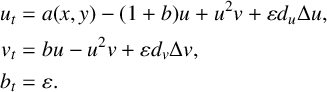 $$ \begin{align} \begin{aligned} u_t &= a (x,y) -(1+b)u + u^2 v + \varepsilon d_u \Delta u,\\ v_t &= b u - u^2 v + \varepsilon d_v \Delta v,\\ b_t &= \varepsilon. \end{aligned} \end{align} $$
Here, the independent variables are $(x,y) \in \mathbf {R}^2$
and
$(x,y) \in \mathbf {R}^2$
and $t\ge 0$
,
$t\ge 0$
, $\Delta = ({\partial ^2}/{\partial x^2}) + ({\partial ^2}/{\partial y^2})$
, and the subscript t denotes the partial derivative on t. The dependent variable u denotes the concentration of the activator chemical and v denotes that of the inhibitor species. The small parameter
$\Delta = ({\partial ^2}/{\partial x^2}) + ({\partial ^2}/{\partial y^2})$
, and the subscript t denotes the partial derivative on t. The dependent variable u denotes the concentration of the activator chemical and v denotes that of the inhibitor species. The small parameter $0<\varepsilon \ll 1$
measures the separation in the time scales. The spatially dependent source term,
$0<\varepsilon \ll 1$
measures the separation in the time scales. The spatially dependent source term, $a(x,y)$
, is taken to be positive, bounded,
$a(x,y)$
, is taken to be positive, bounded, $\mathcal {O}(1)$
with respect to
$\mathcal {O}(1)$
with respect to $\varepsilon $
and smooth. The parameter
$\varepsilon $
and smooth. The parameter $b>0$
denotes a rate constant that slowly increases in time, and
$b>0$
denotes a rate constant that slowly increases in time, and $d_u, d_v>0$
are the diffusivities of the activator and inhibitor.
$d_u, d_v>0$
are the diffusivities of the activator and inhibitor.
5.1. Hopf bifurcation of the QSS
The Brusselator PDE (5.1) has a QSS,
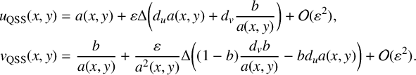 $$ \begin{align*} \begin{aligned} u_{\mathrm{QSS}}(x,y) &= a(x,y) + \varepsilon \Delta \bigg( d_u a(x,y) + d_v \frac{b}{a(x,y)} \bigg) + \mathcal{O}(\varepsilon^2), \\ v_{\mathrm{QSS}}(x,y) &= \frac{b}{a(x,y)} + \frac{\varepsilon}{a^2(x,y)} \Delta \bigg((1-b) \frac{d_v b}{a(x,y)}-b d_u a(x,y) \bigg) + \mathcal{O}(\varepsilon^2). \end{aligned} \end{align*} $$
We perform a linear stability analysis about the QSS by setting $u=u_{\mathrm {QSS}} + \hat {u}$
and
$u=u_{\mathrm {QSS}} + \hat {u}$
and ${v = v_{\mathrm {QSS}} + \hat {v}}$
. The linearized system for
${v = v_{\mathrm {QSS}} + \hat {v}}$
. The linearized system for $\hat {u}$
and
$\hat {u}$
and $\hat {v}$
is
$\hat {v}$
is
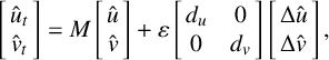 $$ \begin{align*} \left[\!\!\begin{array}{c} \hat{u}_t \\ \hat{v}_t \end{array}\!\!\right] = M \left[\!\!\begin{array}{c} \hat{u} \\ \hat{v} \end{array}\!\!\right] + \varepsilon \left[\!\!\begin{array}{cc} d_u & 0 \\ 0 & d_v \end{array}\!\!\right] \left[\!\! \begin{array}{c} \Delta \hat{u} \\ \Delta \hat{v} \end{array}\!\!\right], \end{align*} $$
where
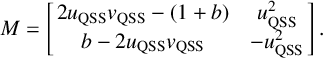 $$ \begin{align*} M = \left[\!\!\begin{array}{cc} 2 u_{\mathrm{QSS}} v_{\mathrm{QSS}} - (1+b) & u_{\mathrm{QSS}}^2 \\ b - 2 u_{\mathrm{QSS}} v_{\mathrm{QSS}} & - u_{\mathrm{QSS}}^2 \end{array}\!\!\right]. \end{align*} $$
Hence, by setting $\mathrm {Tr}(M)=0$
, we find that the PDE (5.1) exhibits a spatially dependent Hopf bifurcation at
$\mathrm {Tr}(M)=0$
, we find that the PDE (5.1) exhibits a spatially dependent Hopf bifurcation at $b = b_H(x,y) $
, where
$b = b_H(x,y) $
, where
 $$ \begin{align} b_H (x,y) = \frac{1 + a^2 + 2 \varepsilon a d_u \Delta a + \mathcal{O}(\varepsilon^2)} {1 + 2\varepsilon d_v ((1-a^2)/a) \Delta ({1}/{a}) + \mathcal{O}(\varepsilon^2) }, \end{align} $$
and we have written a for $a(x,y)$
. At each point
$a(x,y)$
. At each point $(x,y) \in \mathbf {R}^2$
, the QSS is linearly stable for
$(x,y) \in \mathbf {R}^2$
, the QSS is linearly stable for $b < b_H(x,y)$
and linearly unstable for
$b < b_H(x,y)$
and linearly unstable for $b>b_H(x,y)$
. Moreover, the frequency,
$b>b_H(x,y)$
. Moreover, the frequency, $\omega _H$
, at
$\omega _H$
, at $b_H$
is
$b_H$
is $\omega _H = a(x,y)+\mathcal {O}(\varepsilon )$
.
$\omega _H = a(x,y)+\mathcal {O}(\varepsilon )$
.
Remark 4 The Brusselator model (5.1) exhibits (super-critical) Turing bifurcations. For example, with source $a(x,y)=a_0 + \varepsilon a_1(x,y) + \mathcal {O}(\varepsilon ^2)$
, where
$a(x,y)=a_0 + \varepsilon a_1(x,y) + \mathcal {O}(\varepsilon ^2)$
, where $a_0>0$
and
$a_0>0$
and $\mathcal {O}(1)$
, Turing bifurcations occur at
$\mathcal {O}(1)$
, Turing bifurcations occur at $b_T=( 1 \pm \sqrt {{d_u}/{d_v}} a_0)^2 + \mathcal {O}(\varepsilon )$
, in which spatially periodic states are created. The parameter values here were chosen so the Turing bifurcations do not have an impact on the DHB phenomenon. It would be of interest to study the interactions between the two bifurcations.
$b_T=( 1 \pm \sqrt {{d_u}/{d_v}} a_0)^2 + \mathcal {O}(\varepsilon )$
, in which spatially periodic states are created. The parameter values here were chosen so the Turing bifurcations do not have an impact on the DHB phenomenon. It would be of interest to study the interactions between the two bifurcations.
5.2. Spatio-temporal dependence of the DHB in the Brusselator model
In this section, we present the results of numerical simulations showing the spatio-temporal dependence of the DHB in the Brusselator model (5.1). We take the initial values $b(t_0)< b_H(x,y)$
for all
$b(t_0)< b_H(x,y)$
for all $(x,y)$
, so that the system slowly passes through the Hopf bifurcation
$(x,y)$
, so that the system slowly passes through the Hopf bifurcation $b_H(x,y)$
as b slowly increases (recall (5.2)). We work with a stripe source term,
$b_H(x,y)$
as b slowly increases (recall (5.2)). We work with a stripe source term,
 $$ \begin{align} a_S(x,y) = 1+ \varepsilon \alpha \sum_k [ H(x-x_k)-H(x-(x_k+h))], \end{align} $$
where $\alpha>0$
,
$\alpha>0$
, $x_k$
denotes the left edge of the kth stripe,
$x_k$
denotes the left edge of the kth stripe, $x_{k+1}-x_k=\Delta $
,
$x_{k+1}-x_k=\Delta $
, $h<\Delta $
is the width of the stripe and the stripes are sufficiently well separated.
$h<\Delta $
is the width of the stripe and the stripes are sufficiently well separated.
In the simulations, the solutions rapidly approach the attracting QSS for $b < b_H(x,y)$
and, after the instantaneous Hopf point is crossed, they stay near the repelling QSS for long times, of
$b < b_H(x,y)$
and, after the instantaneous Hopf point is crossed, they stay near the repelling QSS for long times, of $\mathcal {O}(1/\varepsilon )$
in the fast time t. This is the delay in the Hopf bifurcation, and the solutions leave a neighbourhood of the QSS in a spatially dependent manner. Moreover, they do so by making a large rapid jump, so that there is a hard onset of large-amplitude oscillations.
$\mathcal {O}(1/\varepsilon )$
in the fast time t. This is the delay in the Hopf bifurcation, and the solutions leave a neighbourhood of the QSS in a spatially dependent manner. Moreover, they do so by making a large rapid jump, so that there is a hard onset of large-amplitude oscillations.
For the representative simulation shown in Figure 6, we set $\alpha =5$
,
$\alpha =5$
, $h=0.1$
,
$h=0.1$
, $x_0=-0.05$
and
$x_0=-0.05$
and $\Delta =0.3$
. The initial data is spatially periodic,
$\Delta =0.3$
. The initial data is spatially periodic,
 $$ \begin{align} u_0(x,y)=a(x,y) + 0.5 \cos(\pi^2 x y),\quad v_0(x,t)= \frac{b_0}{a(x,y)} + \varepsilon. \end{align} $$
The initial value of the parameter is $b_0=b(t_0)=1.5$
(Figure 6(a)), below the Hopf point
$b_0=b(t_0)=1.5$
(Figure 6(a)), below the Hopf point $b_H=2$
here. As b slowly increases, the solution rapidly approaches the attracting QSS, and the component of the solution given by the spatially periodic initial data decreases. By the time
$b_H=2$
here. As b slowly increases, the solution rapidly approaches the attracting QSS, and the component of the solution given by the spatially periodic initial data decreases. By the time $b=1.7$
, the remnant of the initial data is faint (Figure 6(b)). Then, when b reaches
$b=1.7$
, the remnant of the initial data is faint (Figure 6(b)). Then, when b reaches $b_H=2$
, there is no visible trace of the initial data (Figure 6(c)).
$b_H=2$
, there is no visible trace of the initial data (Figure 6(c)).
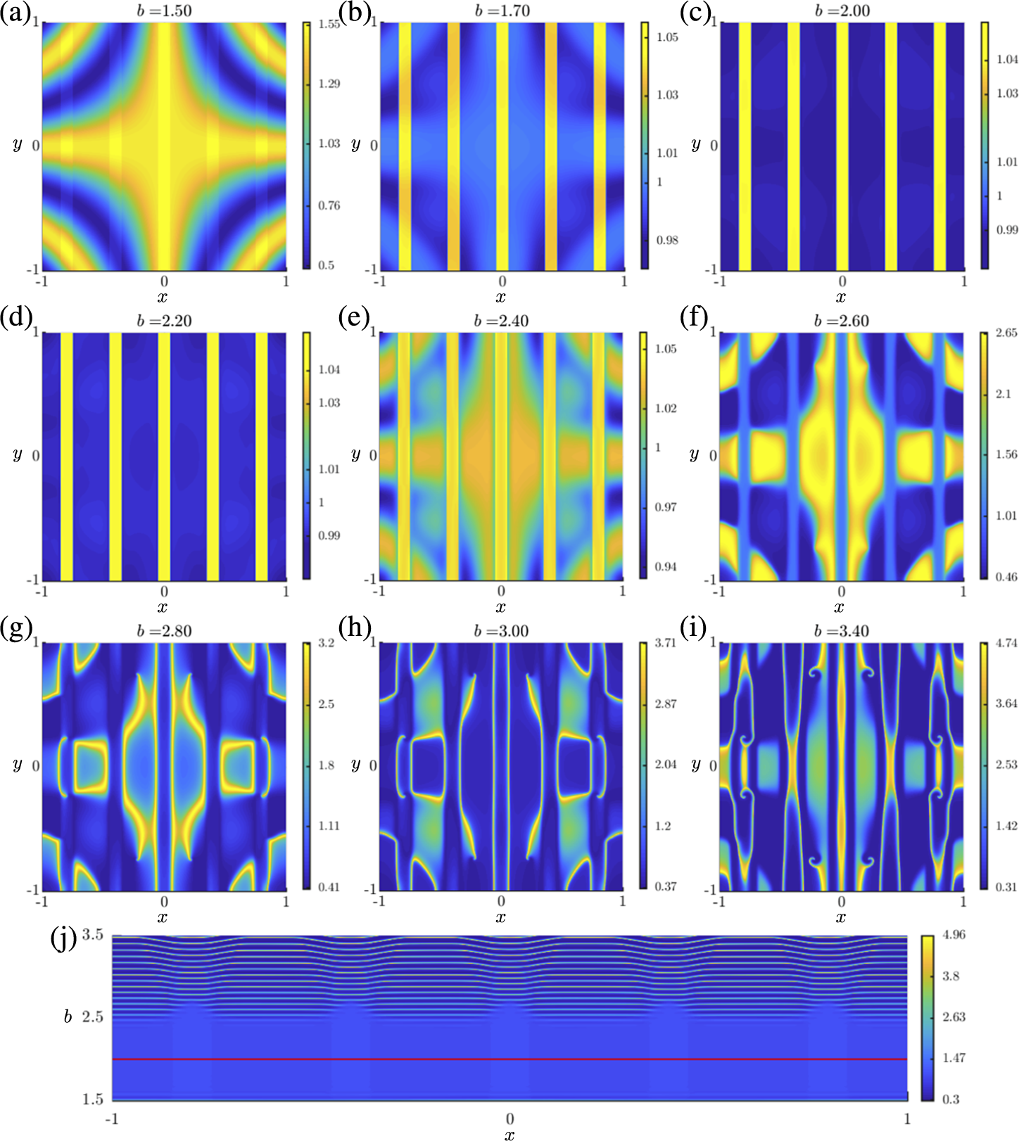
Figure 6 DHB in the two-dimensional Brusselator with stripe source (5.3) and spatially periodic initial data (5.4) given at $b(t_0)=1.5$
. (a)–(i) The solution
$b(t_0)=1.5$
. (a)–(i) The solution $u(x,y)$
rapidly converges to the source-dependent QSS, stays close to the QSS well beyond the instantaneous Hopf bifurcation at
$u(x,y)$
rapidly converges to the source-dependent QSS, stays close to the QSS well beyond the instantaneous Hopf bifurcation at $b=2$
and exhibits a hard transition to oscillations. Note the different scales on the vertical colour bars in panels (a)–(i). (j) Space-time evolution along
$b=2$
and exhibits a hard transition to oscillations. Note the different scales on the vertical colour bars in panels (a)–(i). (j) Space-time evolution along $y=0$
. The parameters are
$y=0$
. The parameters are $\varepsilon = 0.01, d_u = 1 \times 10^{-3}$
,
$\varepsilon = 0.01, d_u = 1 \times 10^{-3}$
, $d_v = 5 \times 10^{-4}$
,
$d_v = 5 \times 10^{-4}$
, $\alpha =5$
,
$\alpha =5$
, $h=0.1$
,
$h=0.1$
, $x_0=-0.05$
and
$x_0=-0.05$
and $\Delta =x_{k+1}-x_k=0.4$
.
$\Delta =x_{k+1}-x_k=0.4$
.
As b continues to increase, the solution remains near the repelling QSS (Figure 6(d), where $b=2.2$
). It is not until
$b=2.2$
). It is not until $b=2.4$
that small amplitude temporal (post-Hopf) oscillations set in (Figure 6(e)). Also, the solution has regained a significant component given by the initial data. The oscillations rapidly gain large amplitude as b increases further (Figure 6(f)–(h), where
$b=2.4$
that small amplitude temporal (post-Hopf) oscillations set in (Figure 6(e)). Also, the solution has regained a significant component given by the initial data. The oscillations rapidly gain large amplitude as b increases further (Figure 6(f)–(h), where $b=2.6$
,
$b=2.6$
, $b=2.8$
,
$b=2.8$
, $b=3.0$
; note the changes in the vertical scales). Hence, the observed onset is a hard onset. Also, significant interactions occur between the components coming from the initial data and the stripe source.
$b=3.0$
; note the changes in the vertical scales). Hence, the observed onset is a hard onset. Also, significant interactions occur between the components coming from the initial data and the stripe source.
Further increases in b result in spatio-temporal patterns, such as spiral waves (Figure 6(i)). These arise from the interaction of the oscillations (which occur beyond the memory surface), the stripe source and the diffusion.
A cross-section through $y=0$
is shown in Figure 6(j). The space-time plot shows that the solution stays close to the QSS (blue state) well past the instantaneous Hopf bifurcation (red line) and the large-amplitude oscillations do not set in until
$y=0$
is shown in Figure 6(j). The space-time plot shows that the solution stays close to the QSS (blue state) well past the instantaneous Hopf bifurcation (red line) and the large-amplitude oscillations do not set in until $b \approx 2.5$
. Cross-sections taken at other values of y are qualitatively the same, with some slight shifts in x.
$b \approx 2.5$
. Cross-sections taken at other values of y are qualitatively the same, with some slight shifts in x.
The hard onset of oscillations occurs along the escape surface, $b_{\mathrm {esc}}(x,y)$
, which at each point
$b_{\mathrm {esc}}(x,y)$
, which at each point $(x,y)$
is given by the value of b at which
$(x,y)$
is given by the value of b at which
 $$ \begin{align*}|(u(x,y),v(x,y))-(u_{\mathrm{QSS}}(x,y),v_{\mathrm{QSS}}(x,y))| = \delta_{\mathrm{th}}.\end{align*} $$
This is the analogue of $\mu _{\mathrm {esc}}(x,y)$
. Plots of
$\mu _{\mathrm {esc}}(x,y)$
. Plots of $b_{\mathrm {esc}}(x,y)$
are shown for two different initial values:
$b_{\mathrm {esc}}(x,y)$
are shown for two different initial values: $b(t_0)=0.1$
in Figure 7(a) and
$b(t_0)=0.1$
in Figure 7(a) and $b(t_0)=1.5$
in Figure 7(b). Here, the parameters are the same as in Figure 6. These escape surfaces reveal that the spatio-temporal buffer surface (defined by the particular solution of the equation linearized about the QSS) and the spatio-temporal memory surface (defined by the homogeneous solution) play similar roles here for (5.1). For initial values
$b(t_0)=1.5$
in Figure 7(b). Here, the parameters are the same as in Figure 6. These escape surfaces reveal that the spatio-temporal buffer surface (defined by the particular solution of the equation linearized about the QSS) and the spatio-temporal memory surface (defined by the homogeneous solution) play similar roles here for (5.1). For initial values $b(t_0)$
far from
$b(t_0)$
far from $b_H=2$
, as in Figure 7(a), the escape surface is determined entirely by the stripe source and, hence, by the particular solution. The initial data has no influence on
$b_H=2$
, as in Figure 7(a), the escape surface is determined entirely by the stripe source and, hence, by the particular solution. The initial data has no influence on $b_{\mathrm {esc}}(x,y)$
, because the escape surface is almost invariant. Indeed, this was verified across four different choices of
$b_{\mathrm {esc}}(x,y)$
, because the escape surface is almost invariant. Indeed, this was verified across four different choices of $b(t_0)$
. Then, for initial values of
$b(t_0)$
. Then, for initial values of $b(t_0)$
close to
$b(t_0)$
close to $b_H$
(as in (b)), the escape surface is located below the buffer surface at all points. The homogeneous solution determines the exit time for all
$b_H$
(as in (b)), the escape surface is located below the buffer surface at all points. The homogeneous solution determines the exit time for all $(x,y)$
. The earliest escape times (dark blue regions) are where the initial data has its smallest amplitude (in the hyperbolic bands with the minima of the cosine term) and the light blue hyperbolic bands occur where the cosine term is maximal. In the regions of the stripes, the initial data is larger and the hard onset occurs later, although still before the buffer surface.
$(x,y)$
. The earliest escape times (dark blue regions) are where the initial data has its smallest amplitude (in the hyperbolic bands with the minima of the cosine term) and the light blue hyperbolic bands occur where the cosine term is maximal. In the regions of the stripes, the initial data is larger and the hard onset occurs later, although still before the buffer surface.
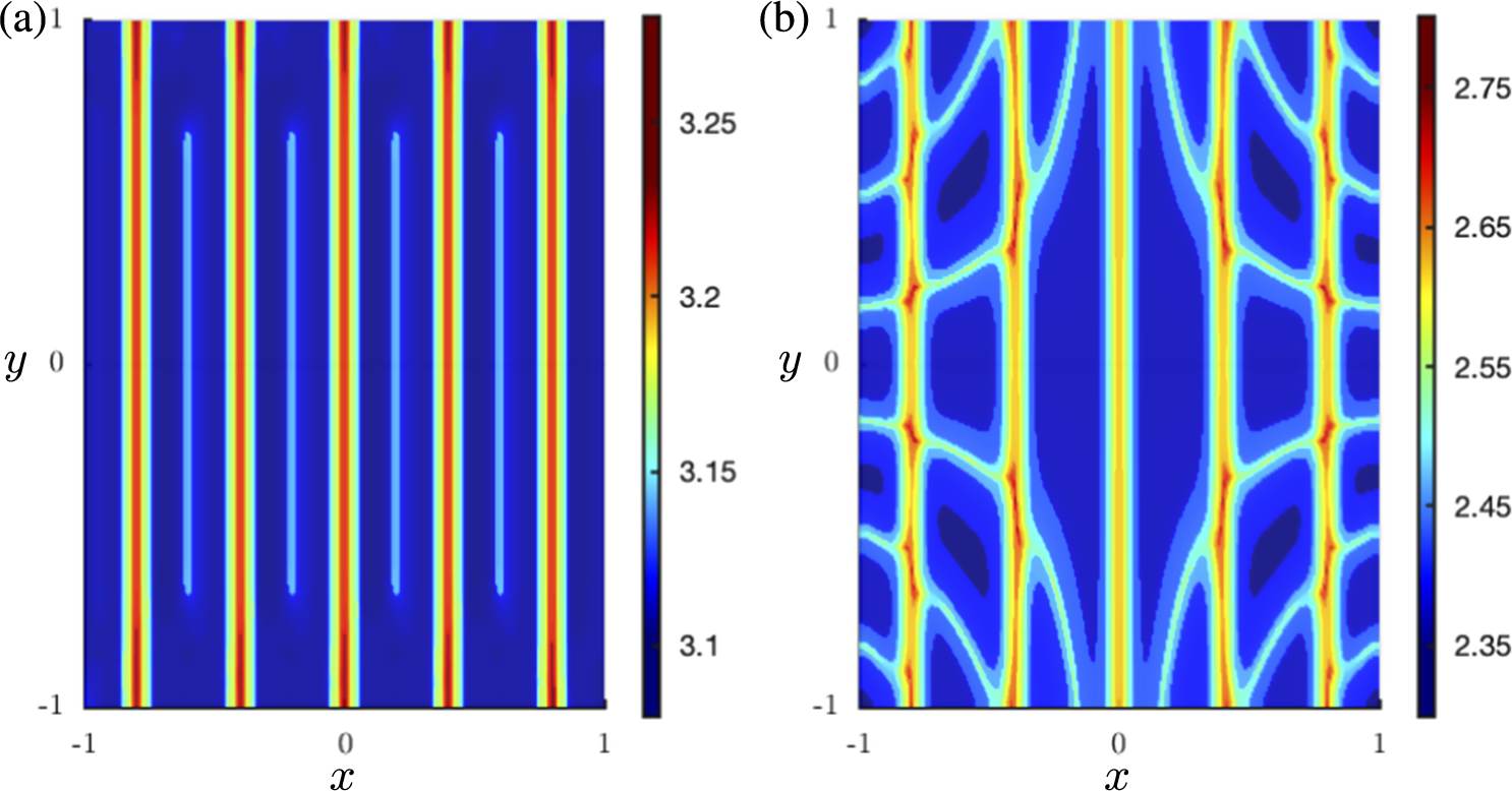
Figure 7 Contours of the escape surface, $b_{\mathrm {esc}}(x,y)$
, where the hard onset of oscillations occurs. The parameters are as in Figure 6 with different values of b at the initial time
$b_{\mathrm {esc}}(x,y)$
, where the hard onset of oscillations occurs. The parameters are as in Figure 6 with different values of b at the initial time $t_0$
:
$t_0$
: $b(t_0)=0.1$
(a) and
$b(t_0)=0.1$
(a) and $b(t_0)=1.5$
(b). The escape surface in (a) depends only on the stripe source and has no memory of the initial data. Similar escape surfaces to (a) are observed for
$b(t_0)=1.5$
(b). The escape surface in (a) depends only on the stripe source and has no memory of the initial data. Similar escape surfaces to (a) are observed for $b(t_0)=0, 0.2$
and
$b(t_0)=0, 0.2$
and $0.3$
. The escape surface in (b) depends on the initial profile.
$0.3$
. The escape surface in (b) depends on the initial profile.
Overall, we find that these primary features of DHBs in the two-dimensional Brusselator—the long, spatially dependent DHB; the hard, spatially dependent onset of large-amplitude oscillations; and the properties of the escape surface—are the same as those observed for DHBs in the CGL PDE in two dimensions (Section 4), as well as for DHBs in PDEs in one dimension [Reference Avitabile, Desroches, Veltz and Wechselberger3, Reference Goh, Kaper and Vo17, Reference Kaper and Vo25], in analytic ODEs [Reference Baer, Erneux and Rinzel4, Reference Hayes, Kaper, Szmolyan and Wechselberger20, Reference Neishtadt35–Reference Neishtadt and Treschev39, Reference Shishkova44, Reference Su46, Reference Su, Jones and Khibnik47] and in the applications cited in the Introduction.
6. Conclusions
In this paper, we studied a pair of prototypical pattern-forming PDEs in two space dimensions. In both, an attracting QSS becomes a repelling QSS as a key parameter varies slowly in time through a generic, super-critical Hopf bifurcation. We reported the discovery of DHBs in which solutions of these PDEs in two dimensions stay near the (post-Hopf) repelling QSS for long, spatially dependent periods of time ( $\mathcal {O}(1/\varepsilon )$
fast time), before the spatially dependent hard onset of large-amplitude oscillations occurs.
$\mathcal {O}(1/\varepsilon )$
fast time), before the spatially dependent hard onset of large-amplitude oscillations occurs.
First, we generalized the asymptotic and numerical results of [Reference Goh, Kaper and Vo17] for DHBs in the CGL PDE in one space dimension to two dimensions. We introduced the spatio-temporal memory surface $\mu _{\mathrm {mem}}(x,y)$
and the spatio-temporal buffer surface
$\mu _{\mathrm {mem}}(x,y)$
and the spatio-temporal buffer surface $\mu _{\mathrm {buf}}(x,y)$
, and we derived asymptotic formulas for them in the CGL PDE (recall Sections 3.1 and 3.2). These are the two-dimensional analogues of the one-dimensional memory and buffer curves introduced in [Reference Goh, Kaper and Vo17].
$\mu _{\mathrm {buf}}(x,y)$
, and we derived asymptotic formulas for them in the CGL PDE (recall Sections 3.1 and 3.2). These are the two-dimensional analogues of the one-dimensional memory and buffer curves introduced in [Reference Goh, Kaper and Vo17].
The memory surface $\mu _{\mathrm {mem}}(x,y)$
is determined by when the homogeneous solution of the linearized equation reaches amplitude one, and hence stops being exponentially small. It is labelled the memory surface for the following reason. Although the memory of the initial data fades quickly after the initial time
$\mu _{\mathrm {mem}}(x,y)$
is determined by when the homogeneous solution of the linearized equation reaches amplitude one, and hence stops being exponentially small. It is labelled the memory surface for the following reason. Although the memory of the initial data fades quickly after the initial time $\mu _0<0$
, because the solution rapidly (exponentially in time) approaches the attracting QSS before the instantaneous Hopf bifurcation, the memory of it is not lost. On the contrary, the component of the solution given by the initial data re-emerges (or resurges) in a spatially dependent manner at
$\mu _0<0$
, because the solution rapidly (exponentially in time) approaches the attracting QSS before the instantaneous Hopf bifurcation, the memory of it is not lost. On the contrary, the component of the solution given by the initial data re-emerges (or resurges) in a spatially dependent manner at $\mu _{\mathrm {mem}}(x,y)$
to leading order. The asymptotic formula for
$\mu _{\mathrm {mem}}(x,y)$
to leading order. The asymptotic formula for $\mu _{\mathrm {mem}}(x,y)$
quantifies its dependence on
$\mu _{\mathrm {mem}}(x,y)$
quantifies its dependence on $\mu _0$
and on the spatial structure of the general bounded, smooth initial data
$\mu _0$
and on the spatial structure of the general bounded, smooth initial data $A_0(x,y)$
. We applied it to several structurally different types of data (see (3.2), (3.5) and (3.8)).
$A_0(x,y)$
. We applied it to several structurally different types of data (see (3.2), (3.5) and (3.8)).
The buffer surface $\mu _{\mathrm {buf}}(x,y)$
is determined from the particular solution
$\mu _{\mathrm {buf}}(x,y)$
is determined from the particular solution $A_p(x,y,\mu )$
by when
$A_p(x,y,\mu )$
by when $\lvert G \rvert = 1$
(recall (3.10)). It plays a central role in the dynamics of solutions for which initial data
$\lvert G \rvert = 1$
(recall (3.10)). It plays a central role in the dynamics of solutions for which initial data $A_0(x,y)$
is given at
$A_0(x,y)$
is given at $\mu _0 \le -\omega _0$
. In particular, to leading order, all solutions with initial data given at
$\mu _0 \le -\omega _0$
. In particular, to leading order, all solutions with initial data given at $\mu _0 \le -\omega _0$
, including those on the attracting QSS, leave an
$\mu _0 \le -\omega _0$
, including those on the attracting QSS, leave an $\mathcal {O}(1)$
neighbourhood of the repelling QSS when
$\mathcal {O}(1)$
neighbourhood of the repelling QSS when $\mu $
reaches the buffer surface, irrespective of how large
$\mu $
reaches the buffer surface, irrespective of how large $|\mu _0|$
is; that is, irrespective of far in the distant past the solutions approached the attracting QSS. Furthermore, we derived the asymptotic formula for
$|\mu _0|$
is; that is, irrespective of far in the distant past the solutions approached the attracting QSS. Furthermore, we derived the asymptotic formula for $\mu _{\mathrm {buf}}(x,y)$
, finding its dependence on the frequency
$\mu _{\mathrm {buf}}(x,y)$
, finding its dependence on the frequency $\omega _0$
at the Hopf point and on the spatial structure of general, smooth, bounded source terms. Also, we applied the general formula to the cases of constant, Gaussian, periodic and stripe sources (see (3.13), (3.14), (3.15) and (3.17)).
$\omega _0$
at the Hopf point and on the spatial structure of general, smooth, bounded source terms. Also, we applied the general formula to the cases of constant, Gaussian, periodic and stripe sources (see (3.13), (3.14), (3.15) and (3.17)).
Overall, for solutions of the CGL PDE (2.1) with initial data given at $\mu _0<0$
, we found that the spatially dependent duration of the DHB is given by
$\mu _0<0$
, we found that the spatially dependent duration of the DHB is given by $\mu _{\mathrm {esc}}(x,y) = \mathrm {\min } \{ \mu _{\mathrm {mem}}(x,y), \mu _{\mathrm {buf}} (x,y) \}$
to leading order. Also, we found that there is good quantitative agreement between the asymptotic formulas for
$\mu _{\mathrm {esc}}(x,y) = \mathrm {\min } \{ \mu _{\mathrm {mem}}(x,y), \mu _{\mathrm {buf}} (x,y) \}$
to leading order. Also, we found that there is good quantitative agreement between the asymptotic formulas for $\mu _{\mathrm { mem}}(x,y)$
and
$\mu _{\mathrm { mem}}(x,y)$
and $\mu _{\mathrm {buf}}(x,y)$
and the numerically calculated escape times
$\mu _{\mathrm {buf}}(x,y)$
and the numerically calculated escape times $\mu _{\mathrm {esc}} (x,y)$
for different types of initial data and source terms (see Section 4).
$\mu _{\mathrm {esc}} (x,y)$
for different types of initial data and source terms (see Section 4).
We distinguished between the DHBs observed for solutions with initial data given at $\mu _0 \in (-\omega _0,0)$
and for those with initial data given at
$\mu _0 \in (-\omega _0,0)$
and for those with initial data given at $\mu _0 \le -\omega _0$
. For the former (
$\mu _0 \le -\omega _0$
. For the former ( $\mu _0 \in (-\omega _0,0)$
), there are points at which the memory surface is reached before the buffer surface. We have shown examples where the entire memory surface lies below the buffer surface in three dimensions: that is,
$\mu _0 \in (-\omega _0,0)$
), there are points at which the memory surface is reached before the buffer surface. We have shown examples where the entire memory surface lies below the buffer surface in three dimensions: that is, $\mu _{\mathrm {mem}}(x,y) < \mu _{\mathrm {buf}}(x,y)$
for all
$\mu _{\mathrm {mem}}(x,y) < \mu _{\mathrm {buf}}(x,y)$
for all $(x,y)$
(recall the first and second representative simulations in Section 4.1). There are also examples in which only a portion of the memory surface lies below the buffer surface. In this case,
$(x,y)$
(recall the first and second representative simulations in Section 4.1). There are also examples in which only a portion of the memory surface lies below the buffer surface. In this case, $A_0(x,y)$
is such that
$A_0(x,y)$
is such that $\mu _{\mathrm {mem}}(x,y)$
grows with
$\mu _{\mathrm {mem}}(x,y)$
grows with $\Vert (x,y) \Vert $
and then exceeds
$\Vert (x,y) \Vert $
and then exceeds $\mu _{\mathrm {buf}}(x,y)$
on some part of the domain, since
$\mu _{\mathrm {buf}}(x,y)$
on some part of the domain, since $\varepsilon $
has a small but finite value.
$\varepsilon $
has a small but finite value.
For the latter (where $\mu _0 \le -\omega _0$
), the buffer surface is reached first as
$\mu _0 \le -\omega _0$
), the buffer surface is reached first as $\mu $
slowly increases. That is, there are points
$\mu $
slowly increases. That is, there are points $(x,y)$
at which
$(x,y)$
at which $\mu _{\mathrm {buf}}(x,y) \le \mu _{\mathrm {mem}}(x,y)$
(noting that equality can arise when
$\mu _{\mathrm {buf}}(x,y) \le \mu _{\mathrm {mem}}(x,y)$
(noting that equality can arise when $\mu _0=-\omega _0$
). Crucially, there are two cases: (1)
$\mu _0=-\omega _0$
). Crucially, there are two cases: (1) $\mu _{\mathrm {buf}}(x,y) \le \mu _{\mathrm {mem}}(x,y)$
for all
$\mu _{\mathrm {buf}}(x,y) \le \mu _{\mathrm {mem}}(x,y)$
for all $(x,y)$
and (2)
$(x,y)$
and (2) $\mu _{\mathrm {buf}}(x,y) \le \mu _{\mathrm {mem}}(x,y)$
in some regions while
$\mu _{\mathrm {buf}}(x,y) \le \mu _{\mathrm {mem}}(x,y)$
in some regions while $\mu _{\mathrm {mem}}(x,y) < \mu _{\mathrm {buf}}(x,y)$
in the complementary regions. The example in Section 4.3 illustrates case (1), and an example of case (2) is given in Section 4.2. In case (2), the source term is such that it grows with
$\mu _{\mathrm {mem}}(x,y) < \mu _{\mathrm {buf}}(x,y)$
in the complementary regions. The example in Section 4.3 illustrates case (1), and an example of case (2) is given in Section 4.2. In case (2), the source term is such that it grows with $\Vert (x,y) \Vert $
and then exceeds
$\Vert (x,y) \Vert $
and then exceeds $\mu _{\mathrm { mem}}(x,y)$
on some part of the domain. In all simulations, we found
$\mu _{\mathrm { mem}}(x,y)$
on some part of the domain. In all simulations, we found $\mu _{\mathrm {esc}}(x,y) \approx \mathrm {\min } \{ \mu _{\mathrm {mem}}(x,y), \mu _{\mathrm {buf}}(x,y) \}$
.
$\mu _{\mathrm {esc}}(x,y) \approx \mathrm {\min } \{ \mu _{\mathrm {mem}}(x,y), \mu _{\mathrm {buf}}(x,y) \}$
.
Finally, we showed numerically that DHB occurs in the Brusselator model in two space dimensions. For several source terms $a(x,y)$
, the solutions spend spatially dependent,
$a(x,y)$
, the solutions spend spatially dependent, $\mathcal {O}(1/\varepsilon )$
long times near the repelling QSS. Also, the spatially dependent onset of oscillations is a hard onset, as shown, for example, in going from Figure 6(e) to (f), where we note the change in scales. Moreover, after the oscillations have set in, there are dynamically complex interactions between the source term and the re-emergent component given by the initial data.
$\mathcal {O}(1/\varepsilon )$
long times near the repelling QSS. Also, the spatially dependent onset of oscillations is a hard onset, as shown, for example, in going from Figure 6(e) to (f), where we note the change in scales. Moreover, after the oscillations have set in, there are dynamically complex interactions between the source term and the re-emergent component given by the initial data.
Looking ahead, we observe that it may be possible to extend the results for the CGL PDE in two dimensions to include some source terms $I_a(x,y)$
that are not strictly positive or bounded. For example, in Section 8 of [Reference Goh, Kaper and Vo17], we showed that the asymptotics for the buffer curve in the one-dimensional CGL PDE extend to include bounded sign-changing source terms (such as
$I_a(x,y)$
that are not strictly positive or bounded. For example, in Section 8 of [Reference Goh, Kaper and Vo17], we showed that the asymptotics for the buffer curve in the one-dimensional CGL PDE extend to include bounded sign-changing source terms (such as $\cos (x)$
) and even some algebraically growing source terms (quadratic in space), and that the asymptotics still agree well with the results of numerical simulations in one dimension. Also, it may be possible to extend the results to include large-amplitude source terms and
$\cos (x)$
) and even some algebraically growing source terms (quadratic in space), and that the asymptotics still agree well with the results of numerical simulations in one dimension. Also, it may be possible to extend the results to include large-amplitude source terms and $\mathcal {O}(1)$
diffusivity, as was done for the one-dimensional CGL PDE in [Reference Goh, Kaper and Vo17, Sections 9 and 10].
$\mathcal {O}(1)$
diffusivity, as was done for the one-dimensional CGL PDE in [Reference Goh, Kaper and Vo17, Sections 9 and 10].
We think it would be of interest to put the Brusselator PDE (5.1) into normal form for dynamic super-critical Hopf bifurcation, and to carry out an analysis of the linearized equation in the complex time plane similar to that done for the CGL PDE (2.1) in two dimensions. It would be of interest to determine where the saddle points are and where the Stokes lines through them cross the real time axis, as well as to derive the homogeneous and particular solutions of the linearized equation and hence determine the spatio-temporal memory and buffer surfaces.
The spatially dependent source terms studied here are similar to those studied in reaction–diffusion equations in two (or more) spatial variables. In [Reference Kollar and Scheel27], the authors established the conditions under which radially symmetric inhomogeneities create coherent structures, including sources, contact defects and sinks. Also, spatial inhomogeneities have been analysed in the Swift–Hohenberg and Ginzburg–Landau equations in two dimensions in [Reference Jaramillo, Scheel and Wu23] and the references therein. The authors demonstrate the existence of weakly deformed stripe patterns, which are small perturbations of the uniform vertical stripes, where the small parameter measures the amplitude of the spatial inhomogeneity. Although these studies are for fixed parameters, it might be of interest to study the spatio-temporal dynamics that result from the interactions between these types of heterogeneities and the slow passage of a parameter through a Hopf bifurcation.
Appendix A. Calculation of
$A_p(x,y,\mu )$
using the saddle point method

In this appendix, we apply the saddle point method to find the asymptotic formula (2.5) for the particular solution $A_p(x,y,\mu )$
of the linearized CGL PDE. In the complex
$A_p(x,y,\mu )$
of the linearized CGL PDE. In the complex ${\tilde {\mu }}$
plane (
${\tilde {\mu }}$
plane ( ${\tilde {\mu }}= {\tilde {\mu }}_R + i {\tilde {\mu }}_I$
), the phase function in
${\tilde {\mu }}= {\tilde {\mu }}_R + i {\tilde {\mu }}_I$
), the phase function in $B_p$
is
$B_p$
is
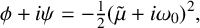 $$ \begin{align*} \phi + i \psi = -\tfrac{1}{2} ( {\tilde{\mu}} + i \omega_0 )^2, \end{align*} $$
where
 $$ \begin{align*} \phi = -\tfrac{1}{2} ( {\tilde{\mu}}_R^2 - ({\tilde{\mu}}_I+\omega_0)^2 )\quad\textrm{and}\quad \psi = - {\tilde{\mu}}_R ({\tilde{\mu}}_I + \omega_0). \end{align*} $$
This phase has a saddle point at ${\tilde {\mu }}=-i\omega _0$
. The level sets of
${\tilde {\mu }}=-i\omega _0$
. The level sets of $\phi $
are hyperbolas and also known as Stokes lines. The Stokes lines with
$\phi $
are hyperbolas and also known as Stokes lines. The Stokes lines with $\phi =0$
through the saddle (which are the asymptotes of the hyperbolas) bound the valleys and hills. They may be parametrized by
$\phi =0$
through the saddle (which are the asymptotes of the hyperbolas) bound the valleys and hills. They may be parametrized by ${\tilde {\mu }}_R$
via
${\tilde {\mu }}_R$
via ${\tilde {\mu }}_I = \pm {\tilde {\mu }}_R - \omega _0.$
Also, the level sets of
${\tilde {\mu }}_I = \pm {\tilde {\mu }}_R - \omega _0.$
Also, the level sets of $\psi $
are hyperbolas (with asymptotes given by the axes), and they are referred to as anti-Stokes lines.
$\psi $
are hyperbolas (with asymptotes given by the axes), and they are referred to as anti-Stokes lines.
Let $\delta>0$
be a small number, independent of
$\delta>0$
be a small number, independent of $\varepsilon $
. We fix an arbitrary value of
$\varepsilon $
. We fix an arbitrary value of ${\mu \in [\delta ,\omega _0]}$
. We consider the contour
${\mu \in [\delta ,\omega _0]}$
. We consider the contour $C_r = C_{r1} \bigcup C_{r2} \bigcup C_{r3} \bigcup C_{r4}$
, where
$C_r = C_{r1} \bigcup C_{r2} \bigcup C_{r3} \bigcup C_{r4}$
, where $C_{r1} = [\mu _0,-\omega _0]$
;
$C_{r1} = [\mu _0,-\omega _0]$
; $C_{r2}$
is the segment of the Stokes line
$C_{r2}$
is the segment of the Stokes line ${\tilde {\mu }}_{I} = - {\tilde {\mu }}_R - \omega _0$
from
${\tilde {\mu }}_{I} = - {\tilde {\mu }}_R - \omega _0$
from $-\omega _0$
down to the saddle at
$-\omega _0$
down to the saddle at $-i\omega _0$
;
$-i\omega _0$
; $C_{r3}$
is the segment of the Stokes line
$C_{r3}$
is the segment of the Stokes line ${\tilde {\mu }}_{I} = {\tilde {\mu }}_R - \omega _0$
from the saddle up to the point
${\tilde {\mu }}_{I} = {\tilde {\mu }}_R - \omega _0$
from the saddle up to the point $q_r=\sqrt {\omega _0\mu } + i (\sqrt {\omega _0\mu }-\omega _0)$
, for this fixed value of
$q_r=\sqrt {\omega _0\mu } + i (\sqrt {\omega _0\mu }-\omega _0)$
, for this fixed value of $\mu $
; and
$\mu $
; and $C_{r4}$
consists of the segment of the steepest ascent curve
$C_{r4}$
consists of the segment of the steepest ascent curve $\psi = -\omega _0\mu $
from
$\psi = -\omega _0\mu $
from $q_r$
up to the point
$q_r$
up to the point $\mu $
(see Figure A.1).
$\mu $
(see Figure A.1).
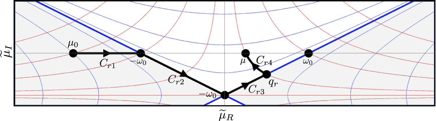
Figure A.1 The contour $C_r = C_{r1} \bigcup C_{r2} \bigcup C_{r3} \bigcup C_{r4}$
in the complex
$C_r = C_{r1} \bigcup C_{r2} \bigcup C_{r3} \bigcup C_{r4}$
in the complex ${\tilde {\mu }}$
plane.
${\tilde {\mu }}$
plane.
We evaluate the integrals in the same manner as in Section 2.3 of [Reference Goh, Kaper and Vo17]. We take any initial $B_p(x,y,\mu _0)$
with
$B_p(x,y,\mu _0)$
with $\mu _0 \le -\omega _0$
on or near the attracting QSS, and we track it along
$\mu _0 \le -\omega _0$
on or near the attracting QSS, and we track it along $C_r$
to the fixed value
$C_r$
to the fixed value $\mu $
. At that point,
$\mu $
. At that point,
 $$ \begin{align*} B_p(x,y,\mu) = \mathcal{I}_{r1} + \mathcal{I}_{r2} + \mathcal{I}_{r3} + \mathcal{I}_{r4}, \end{align*} $$
where, for $\delta \le \mu \le \omega _0$
,
$\delta \le \mu \le \omega _0$
,
 $$ \begin{align*} \mathcal{I}_{rj} = \frac{1}{\sqrt{\varepsilon}} \int_{C_{rj}} g(x,y,\mu - {\tilde{\mu}})e^{-({\tilde{\mu}} + i \omega_0)^2/{2\varepsilon}}\,d{\tilde{\mu}},\quad j=1,2,3,4. \end{align*} $$
The integral $\mathcal {I}_{r1}$
along the segment
$\mathcal {I}_{r1}$
along the segment $C_{r1} = [\mu _0,-\omega _0]$
is evaluated using the method of steepest descents along the contour formed by the union of the Stokes line through
$C_{r1} = [\mu _0,-\omega _0]$
is evaluated using the method of steepest descents along the contour formed by the union of the Stokes line through $\mu =-\mu _0$
out to
$\mu =-\mu _0$
out to $-\infty - i \omega _0$
and the Stokes line back from
$-\infty - i \omega _0$
and the Stokes line back from $-\infty - i \omega _0$
up to
$-\infty - i \omega _0$
up to $\mu =-\omega _0$
.n The dominant contribution comes from the final segment along the latter Stokes line near
$\mu =-\omega _0$
.n The dominant contribution comes from the final segment along the latter Stokes line near $\mu =-\omega _0$
.
$\mu =-\omega _0$
.
 $$ \begin{align} \mathcal{I}_{r1} =\bigg\{\frac{\sqrt{\varepsilon}}{2\omega_0} (1+i) g(x,y,\mu+\omega_0) +\mathcal{O} (\varepsilon^{{3}/{2}}) \bigg\} e^{{i \omega_0^2}/{\varepsilon}}. \end{align} $$
Next, we parametrize $C_{r2}$
by
$C_{r2}$
by ${\tilde {\mu }}_R$
, with
${\tilde {\mu }}_R$
, with ${\tilde {\mu }}_I ({\tilde {\mu }}_R) = - ({\tilde {\mu }}_R + \omega _0)$
and
${\tilde {\mu }}_I ({\tilde {\mu }}_R) = - ({\tilde {\mu }}_R + \omega _0)$
and ${\tilde {\mu }}_R: -\omega _0\to 0$
. Hence,
${\tilde {\mu }}_R: -\omega _0\to 0$
. Hence, $-(\tilde {\mu } + i \omega _0)^2/2= i{\tilde {\mu }}_R^2$
for all
$-(\tilde {\mu } + i \omega _0)^2/2= i{\tilde {\mu }}_R^2$
for all ${\tilde {\mu }}$
on
${\tilde {\mu }}$
on $C_{r2}$
. It is purely imaginary, corresponding to the fact that
$C_{r2}$
. It is purely imaginary, corresponding to the fact that $C_{r2}$
lies on a Stokes line
$C_{r2}$
lies on a Stokes line $\phi =0$
. Hence, for each
$\phi =0$
. Hence, for each ${\tilde {\mu }}$
on
${\tilde {\mu }}$
on $C_{r2}$
, the integrand is of the form to which the method of stationary phase applies; namely,
$C_{r2}$
, the integrand is of the form to which the method of stationary phase applies; namely, $g \cdot e^{({i}/{\operatorname {\mathrm {\varepsilon }}}) h({\tilde {\mu }}_R)}$
with
$g \cdot e^{({i}/{\operatorname {\mathrm {\varepsilon }}}) h({\tilde {\mu }}_R)}$
with $h({\tilde {\mu }}_R)={{\tilde {\mu }}_R}^2$
. Moreover, the end point
$h({\tilde {\mu }}_R)={{\tilde {\mu }}_R}^2$
. Moreover, the end point $\tilde {\mu }=-i\omega _0$
of
$\tilde {\mu }=-i\omega _0$
of $C_{r2}$
(
$C_{r2}$
( ${\tilde {\mu }}_R=0$
) is a point of stationary phase, since
${\tilde {\mu }}_R=0$
) is a point of stationary phase, since $h'(0)=0$
and
$h'(0)=0$
and $h"(0)=2 \ne 0$
, and it is the only such point along
$h"(0)=2 \ne 0$
, and it is the only such point along $C_{r2}$
. (For the general method in which an end point is a saddle (or turning) point, see, for example, Section 4.1 of [Reference Murray34], in particular formula (4.14).)
$C_{r2}$
. (For the general method in which an end point is a saddle (or turning) point, see, for example, Section 4.1 of [Reference Murray34], in particular formula (4.14).)
Applying the method of stationary phase, we insert the parametrization of $C_{r2}$
, use
$C_{r2}$
, use ${\tilde {\nu }}=-{\tilde {\mu }}_R$
, Taylor expand about
${\tilde {\nu }}=-{\tilde {\mu }}_R$
, Taylor expand about ${\tilde {\nu }}=0$
(that is,
${\tilde {\nu }}=0$
(that is, ${\tilde {\mu }}=-i\omega _0$
) and observe that the dominant contribution asymptotically comes from the point of stationary phase at the saddle,
${\tilde {\mu }}=-i\omega _0$
) and observe that the dominant contribution asymptotically comes from the point of stationary phase at the saddle,
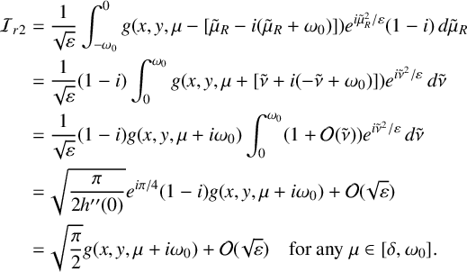 $$ \begin{align} \mathcal{I}_{r2} &= \frac{1}{\sqrt{\varepsilon}} \int_{-\omega_0}^0 g(x,y,\mu - [ {\tilde{\mu}}_R - i({\tilde{\mu}}_R + \omega_0) ])e^{{i}{\tilde{\mu}}_R^2/{\varepsilon} }(1-i)\,d{\tilde{\mu}}_R \nonumber \\ &= \frac{1}{\sqrt{\varepsilon}}(1-i) \int_0^{\omega_0} g(x,y,\mu + [ {\tilde{\nu}} + i(-{\tilde{\nu}} + \omega_0) ])e^{{i}{\tilde{\nu}}^2/{\varepsilon}}\,d{\tilde{\nu}} \nonumber \\ &= \frac{1}{\sqrt{\varepsilon}}(1-i)g(x,y,\mu+i\omega_0)\int_0^{\omega_0}(1 + \mathcal{O}({\tilde{\nu}}))e^{{i}{\tilde{\nu}}^2/{\varepsilon} }\,d{\tilde{\nu}} \nonumber\\ &= \sqrt{\frac{\pi}{2 h"(0)}} e^{{i\pi}/{4}} (1-i) g(x,y,\mu+i\omega_0) + \mathcal{O}(\sqrt{\varepsilon}) \nonumber \\ &= \sqrt{\frac{\pi}{2}} g(x,y,\mu+i\omega_0) + \mathcal{O}(\sqrt{\varepsilon})\quad\text{for any } \mu \in [\delta,\omega_0]. \end{align} $$
This leading order term in $\mathcal {I}_{r2}$
will turn out to be half of the leading order term in the total integral for
$\mathcal {I}_{r2}$
will turn out to be half of the leading order term in the total integral for $B_p(x,y,\mu )$
for each
$B_p(x,y,\mu )$
for each $\mu \in [\delta ,\omega _0]$
.
$\mu \in [\delta ,\omega _0]$
.
Next, we show that $\mathcal {I}_{r3}$
gives the other half of the leading order term in
$\mathcal {I}_{r3}$
gives the other half of the leading order term in $B_p$
. From the definition of
$B_p$
. From the definition of $C_{r3}$
, we have that, for any
$C_{r3}$
, we have that, for any $\mu \in [\delta ,\omega _0]$
,
$\mu \in [\delta ,\omega _0]$
,
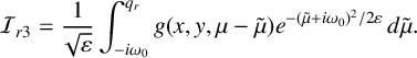 $$ \begin{align*} \mathcal{I}_{r3} = \frac{1}{\sqrt{\varepsilon}} \int_{-i\omega_0}^{q_r} g(x,y,\mu - {\tilde{\mu}}) e^{-(\tilde{\mu} + i \omega_0)^2/{2\varepsilon}}\,d{\tilde{\mu}}. \end{align*} $$
We use ${\tilde {\mu }}_R$
to parametrize
${\tilde {\mu }}_R$
to parametrize $C_{r3}$
as
$C_{r3}$
as ${\tilde {\mu }}_I = {\tilde {\mu }}_R - \omega _0$
, now with
${\tilde {\mu }}_I = {\tilde {\mu }}_R - \omega _0$
, now with ${\tilde {\mu }}_R: 0 \to \sqrt {\omega _0\mu }$
. Hence,
${\tilde {\mu }}_R: 0 \to \sqrt {\omega _0\mu }$
. Hence, ${-(\tilde {\mu } + i \omega _0)^2/2= -i{\tilde {\mu }}_R^2}$
along
${-(\tilde {\mu } + i \omega _0)^2/2= -i{\tilde {\mu }}_R^2}$
along $C_{r3}$
; and, for each
$C_{r3}$
; and, for each ${\tilde {\mu }}$
on
${\tilde {\mu }}$
on $C_{r3}$
, the integral is also of the form to apply the method of stationary phase,
$C_{r3}$
, the integral is also of the form to apply the method of stationary phase, $g \cdot e^{({i}/{\varepsilon }) {\tilde h}(\tilde {\mu }_R)}$
, with
$g \cdot e^{({i}/{\varepsilon }) {\tilde h}(\tilde {\mu }_R)}$
, with ${\tilde h}({\tilde {\mu }_R})=-{\tilde {\mu }}_R^2$
. Moreover, the initial point
${\tilde h}({\tilde {\mu }_R})=-{\tilde {\mu }}_R^2$
. Moreover, the initial point $\tilde {\mu }=-i\omega _0$
of
$\tilde {\mu }=-i\omega _0$
of $C_{r3}$
(
$C_{r3}$
( ${\tilde {\mu }}_R=0$
) is a stationary phase point, since
${\tilde {\mu }}_R=0$
) is a stationary phase point, since ${\tilde h}'(0)=0$
and
${\tilde h}'(0)=0$
and ${\tilde h}"(0)=-2 \ne 0$
, and it is the only such point along
${\tilde h}"(0)=-2 \ne 0$
, and it is the only such point along $C_{r3}$
. We find
$C_{r3}$
. We find
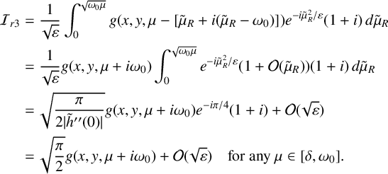 $$ \begin{align} \mathcal{I}_{r3} &= \frac{1}{\sqrt{\varepsilon}} \int_0^{\sqrt{\omega_0\mu}} g(x,y,\mu - [ {\tilde{\mu}}_R + i({\tilde{\mu}}_R - \omega_0) ])e^{-{i} {\tilde{\mu}}_R^2/{\varepsilon}}(1+i)\,d{\tilde{\mu}}_R \nonumber \\ &=\frac{1}{\sqrt{\varepsilon}} g(x,y,\mu+i\omega_0) \int_0^{\sqrt{\omega_0\mu}} e^{-{i} {\tilde{\mu}}_R^2/{\varepsilon}} (1 + \mathcal{O}({\tilde{\mu}}_R)) (1+i)\,d{\tilde{\mu}}_R \nonumber\\ &= \sqrt{\frac{\pi}{2 \vert {\tilde h}"(0)\vert}} g(x,y,\mu+i\omega_0)e^{-{i\pi}/{4}}(1+i) + \mathcal{O}(\sqrt{\varepsilon}) \nonumber \\ &= \sqrt{\frac{\pi}{2}} g(x,y,\mu+i\omega_0) + \mathcal{O}(\sqrt{\varepsilon}) \quad\text{for any } \mu \in [\delta,\omega_0]. \end{align} $$
Finally, we calculate $\mathcal {I}_{r4}$
. Implicitly parametrize
$\mathcal {I}_{r4}$
. Implicitly parametrize $C_{r4}$
using
$C_{r4}$
using $\sigma $
,
$\sigma $
,
 $$ \begin{align*} C_{r4}: \quad -\tfrac{1}{2} ({\tilde{\mu}} + i \omega_0)^2 = -\tfrac{1}{2} (\mu + i \omega_0)^2 + \sigma. \end{align*} $$
The parameter $\sigma $
starts from
$\sigma $
starts from $-(\omega _0^2 - \mu ^2)/2$
at the point
$-(\omega _0^2 - \mu ^2)/2$
at the point $q_r$
and increases monotonically along
$q_r$
and increases monotonically along $C_{r4}$
to zero at
$C_{r4}$
to zero at $\mu $
. The explicit representation is
$\mu $
. The explicit representation is
 $$ \begin{align*} {\tilde{\mu}}(\sigma) = -i\omega_0 + [ (\mu + i \omega_0)^2 - 2\sigma]^{{1}/{2}}. \end{align*} $$
The integration along $C_{r4}$
gives
$C_{r4}$
gives
 $$ \begin{align*} \mathcal{I}_{r4} = \sqrt{\varepsilon} e^{-(\mu+i\omega_0)^2/{2\varepsilon}} \int_{-(\omega_0^2 - \mu^2)/{2}}^{0} \frac{g(x,y,\mu+i\omega_0- [(\mu+i\omega_0)^2 - 2\sigma]^{{1}/{2}}) e^{{\sigma}/{\varepsilon}}} {\sqrt{(\mu + i \omega_0)^2 - 2\sigma}}\,d\sigma. \end{align*} $$
Hence, one finds
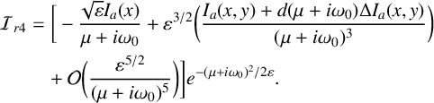 $$ \begin{align} \mathcal{I}_{r4} &= \bigg[ -\frac{\sqrt{\varepsilon} I_a(x)} {\mu+i\omega_0} + \varepsilon^{{3}/{2}} \bigg(\frac{I_a(x,y)+d(\mu+i\omega_0)\Delta I_a(x,y)} {(\mu+i \omega_0)^3} \bigg) \nonumber \\ &\quad + \mathcal{O}\bigg(\frac{\varepsilon^{{5}/{2}}} {(\mu+i\omega_0)^5}\bigg) \bigg] e^{-(\mu+i\omega_0)^2/{2\varepsilon}}. \end{align} $$
Summing (A.1), (A.2), (A.3) and (A.4), we have that, for $\delta \le \mu \le \omega _0$
,
$\delta \le \mu \le \omega _0$
,
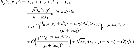 $$ \begin{align*} B_p(x,y,\mu)&=\mathcal{I}_{r1} + \mathcal{I}_{r2} + \mathcal{I}_{r3} + \mathcal{I}_{r4} \\ &= - \frac{\sqrt{\varepsilon} I_a(x,y)}{\mu + i \omega_0}e^{-(\mu+i\omega_0)^2/{2\varepsilon}}\\ &\quad + \varepsilon^{{3}/{2}} \bigg(\frac{I_a(x,y)+d(\mu+i\omega_0)\Delta I_a(x,y)} {(\mu+i \omega_0)^3} \bigg) e^{-(\mu+i\omega_0)^2/{2\varepsilon}} \\ &\quad + \mathcal{O}\bigg(\frac{\varepsilon^{{5}/{2}} e^{-(\mu+i\omega_0)^2/{2\varepsilon}}}{(\mu+i\omega_0)^5}\bigg) + \sqrt{2\pi} g(x,y,\mu+i\omega_0) + \mathcal{O}(\sqrt{\varepsilon}). \end{align*} $$
Finally, we translate the formula back to the dependent variable A, which completes the derivation of (2.5).
Acknowledgements
The authors congratulate Bernd Krauskopf on the occasion of this sixtieth birthday. We are pleased to help honour his many contributions to the fields of bifurcation theory, dynamical systems, delay differential equations, numerical methods for dynamical systems and applications of dynamical systems.
The research of the authors was partially supported by NSF-DMS 2307650 (RG). The authors thank the two anonymous referees for their constructive suggestions, including to add two additional illustrative figures. The authors thank David Barton, Andrus Giraldo, Andrew Keane, James Knowles, Hinke Osinga and Sebastian Wieczorek for organizing the conference “Frontiers in Applied Dynamical Systems” held at the University of Cork, Ireland, June 18–20, 2024, and for editing this issue.


 Open access