Symmetric influence of forward and opposing tidal currents on rogue wave statistics

Abstract

Rogue waves are associated with various ocean processes, both at the coast and in the open ocean. In either zone, inhomogeneities in the wave field caused by shoaling, crossing seas or current interactions disturb the wave statistics, increasing the rogue wave probability and magnitude. Such amplification of the frequency of rogue waves and their intensity, i.e. the maximum normalised height, have been attested to in numerical simulations and laboratory studies, in particular for wave–current interactions. In this study, we investigate the effect of the current intensity and direction on rogue wave probability, by analysing long-term observations from the southern North Sea. We observe that the amplification is similar for opposing and following currents. Despite the sea states being dominantly broadbanded and featuring a large directional spread, the anomalous statistics are of the same order of magnitude as those observed in unidirectional laboratory experiments for stationary currents.

1. Introduction

Waves exceptionally higher than the mean of the highest surrounding ones, so-called rogue waves, have been extensively observed over two decades by buoys (de Pinho, Liu & Parente Ribeiro 2004; Doong & Wu 2010; Cattrell et al. 2018; Häfner et al. 2021), satellite imagery (Rosenthal & Lehner 2007, 2008), oil platform sensors (Haver 2000; Stansell 2004; Mendes, Scotti & Stansell 2021) or a combination thereof (Christou & Ewans 2014; Karmpadakis, Swan & Christou 2020; Teutsch et al. 2020; Teutsch & Weisse 2023). They are generally defined as waves exceeding twice the significant wave height, $H_s$ , which is the mean height of the largest third of the waves in a given sea state. Accidents near the coast of South Africa half a century ago due to the interaction of wave trains travelling in opposition to strong surface currents provided substantial evidence of their existence (Mallory 1974; Smith 1976; Lavrenov 1998). However, they were disregarded, since their existence challenged the linear theory of irregular ocean waves.

Waves in inhomogeneous media have been investigated from a deterministic point of view since the 1940s (Unna 1942; Johnson 1947). Advanced mathematical techniques (Ursell 1960; Whitham 1962, 1965; Bretherton, Garrett & Lighthill 1968) allowed us to assess wave–current interactions through ray theory (Arthur 1950; Whitham 1960; Kenyon 1971), linear wave theory (Taylor 1955; Peregrine 1976), radiation stress (Longuet-Higgins & Stewart 1960, 1961) and spectral (Huang et al. 1972) as well as perturbative methods (McKee 1974). The works of Longuet-Higgins (1952, 1963) on the statistics of interaction-free water waves were conducted in parallel with his work on currents (Longuet-Higgins & Stewart 1960), yet no work extended these statistical analyses to wave–current systems. Although the possibility of the existence of rogue waves was originally raised from wave–current observations (Mallory 1974), the different focus placed by communities working on wave statistics on one side, and on the theoretical fluid dynamics of wave–current systems on the other side, persisted for decades. In fact, the study of how currents affect wave statistics and extreme events came under consideration only recently (White & Fornberg 1998; Heller, Kaplan & Dahlen 2008; Janssen & Herbers 2009). Gemmrich & Garrett (2012) observed an amplification of significant wave heights on following tidal currents. Also Ho, Merrifield & Pizzo (2023) found surface waves to be modified by the tide, depending on the relative speed between the tidal wave and the surface waves. For comparable wave speeds and propagation directions, significant wave heights were amplified. However, the ray theory of wave–current statistics (Heller et al. 2008; Ying et al. 2011) has not been tested against observations or laboratory experiments. Due to their definition relative to the significant wave height rather than an absolute height, the occurrence of rogue waves is independent of the absolute value of any sea state variable, such as significant wave height or mean wavelength (Stansell 2004; Christou & Ewans 2014; Mendes et al. 2021). Therefore, effects of the currents on either the wave height or wavelength cannot be translated into modulations of the rogue wave probability.

In the present work, we focus on the influence of wave–current interaction on wave height statistics. As modulations of wave amplitude and wavenumber are functions of the ratio of the current and wave speeds, respectively, $U/c_{{g}}$ (Longuet-Higgins & Stewart 1960), it seems natural to normalise the current speed with the group velocity of the waves. A proper theoretical study of both wave groups and random wave fields using the nonlinear Schrödinger equation (NLSE) showed good agreement with numerical simulations on the maximum amplitude driven by the interaction of the wave train with opposing currents (Onorato, Proment & Toffoli 2011). Moreover, Toffoli et al. (2013) computed the maximum wave amplitude from the NLSE and found good agreement with unidirectional experiments with opposing currents carried out in two different wave flumes. Further experiments were performed to investigate broadbanded waves with finite directional spreading, demonstrating a decrease in amplification with directionality (Toffoli et al. 2015). As predicted by Onorato et al. (2011) and confirmed experimentally by Toffoli et al. (2015) and Ducrozet et al. (2021), the amplification of the rogue wave probability due to an opposing current is related to the magnitude of the ratio between the current speed and the wave group speed $U/c_g$ .

When dealing with following currents, studies on either wave modulation or wave statistics are scarce. Hjelmervik & Trulsen (2009) were the first to provide evidence that, not only opposing, but also following currents may increase rogue wave occurrence. Recently, simulations performed by Zheng, Li & Ellingsen (2023) and flume experiments by Zhang et al. (2023) have upheld the amplification influence of following currents, although the latter included depth effects of waves travelling over a bar. Halsne et al. (2024) analysed the effect of non-stationary (and/or) non-homogeneous following and opposing currents (or tides) on the maximum height of irregular wave fields, but they did not investigate the probability distributions of wave heights. Generalising these studies to the wave height distribution, our present work aims to investigate how the interaction of waves with both opposing and following currents amplifies rogue wave occurrence under real ocean conditions, i.e. waves of broad spectrum and directional spreading subject to interaction with tidal (non-stationary) currents in the southern North Sea.

2. Data and methods

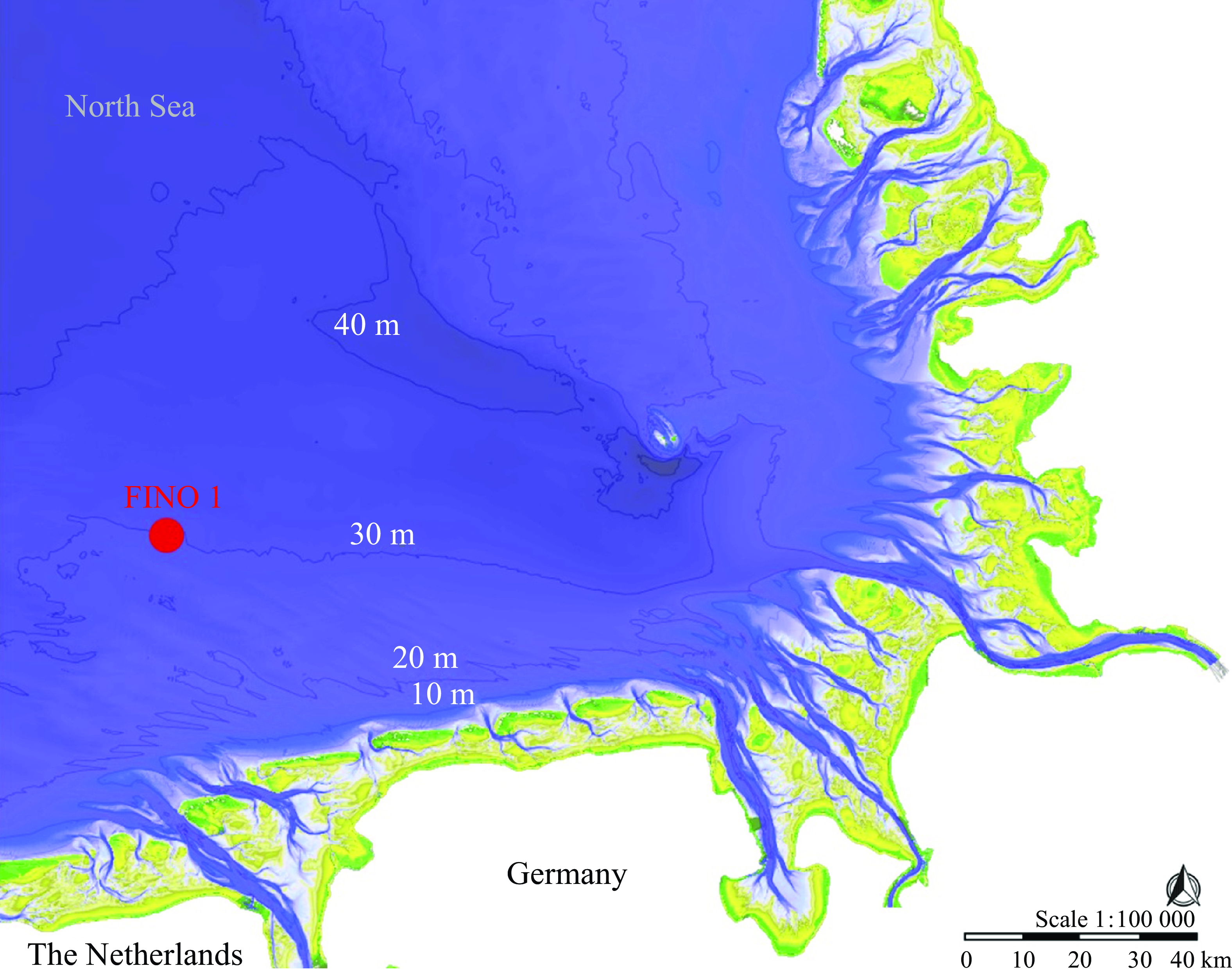
Figure 1. Location of the research platform FINO1 in the southern North Sea, close to the Dutch and German Frisian islands. Data from MDI-DE (2024).

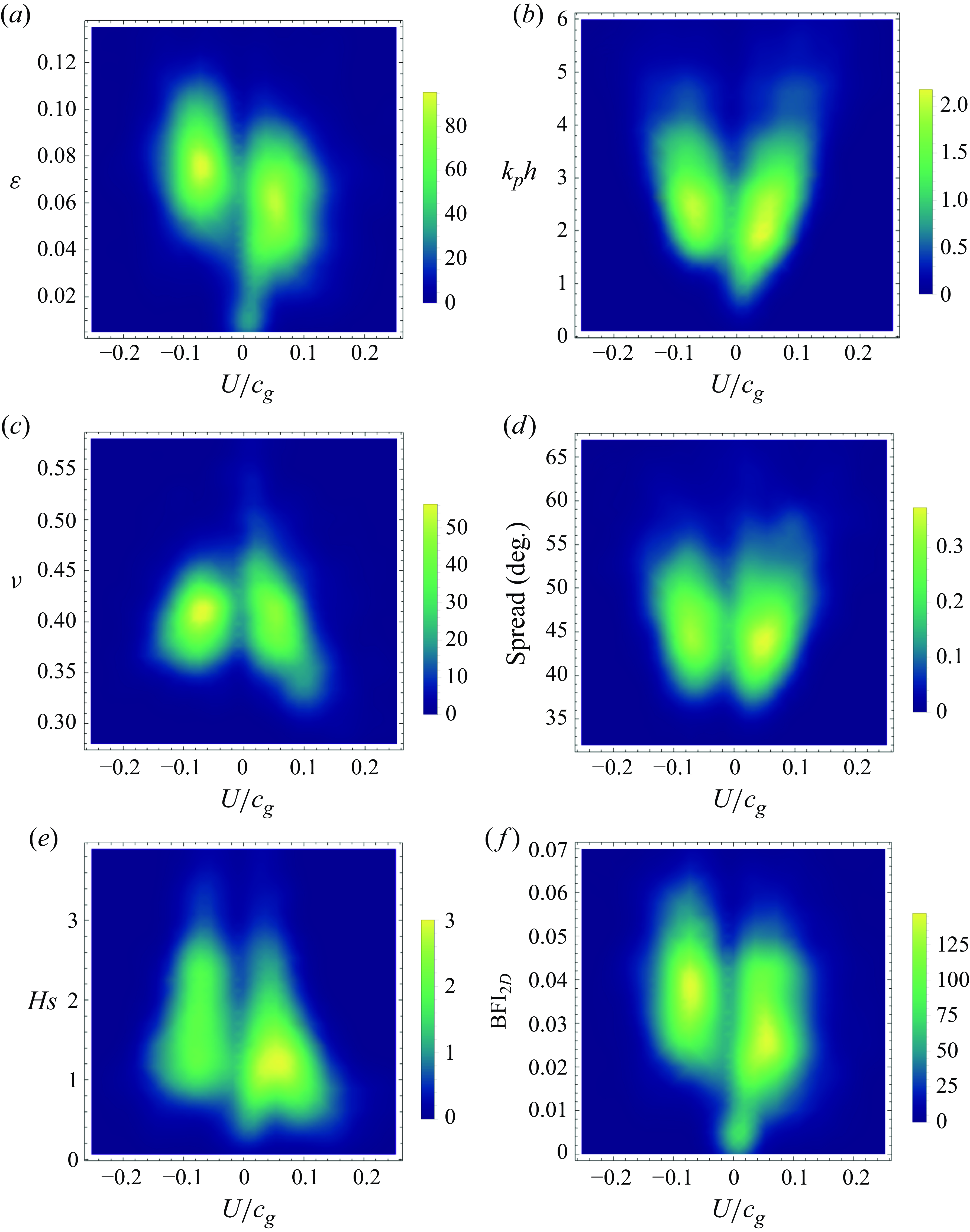
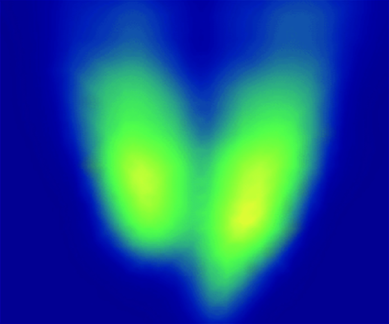
Figure 2. Joint probability densities of several sea parameters and normalised current speed $U/c_{g}$ : (a) mean wave steepness $\varepsilon = (\sqrt {2}/\pi ) k_p H_s$ , (b) relative water depth $k_p h$ , (c) bandwidth $\nu$ (Longuet-Higgins 1975), (d) directional spread $\sigma _{\theta } = \sqrt {2(1+s)}$ for a directional spectral function $D(\theta ) \sim \cos ^{2s}{(\theta /2)}$ , (e) significant wave height and ( f) the two-dimensional Benjamin–Feir index BFI_2D (Mori, Onorato & Janssen 2011).

As described in detail in Teutsch, Mendes & Kasparian (2024), wave and current data were recorded in the southern North Sea (FINO 1 research platform, 54.015 $^{\circ }$ N 6.588 $^{\circ }$ E, 30 m depth), see figure 1, between July 2019 and December 2022. This long sampling period, combined with the fast oscillation of the tidal current ( ${\sim}12$ hours) as compared with most of the factors influencing the variability of the waves, limits the effects of the sampling variability on our analysis. Tidal currents are typically east- and westward, while the waves (of peak frequency 0.11–0.14 Hz) propagated mostly south-southeast- or eastward. Surface elevation was measured at a rate of 1.28 Hz and with a resolution of 0.01 m, in 30 minute long samples. An analysis of the sea conditions showed that tidal currents normalised by the group velocity of the waves $U/c_{{g}}$ range between $-0.225$ and 0.257, with two modes approximately around $\pm 0.05$ , and that stronger tidal currents symmetrically decrease the wavelength and bandwidth and increase the directional spread (Teutsch et al. 2024). Furthermore, moderate currents boost the significant wave height while opposing currents push up the wave steepness. We also underline that, unlike flume experiments, our observations cover a wide range of sea states (figure 2), which is expected to affect the wave statistics (Bitner-Gregersen & Gramstad 2018). When analysing more homogeneous data subsets with narrow ranges of steepness and directional spread, we obtained preliminary indications that data homogeneity may increase the exceedance probability in the presence of a current and lower it in rest conditions, resulting in stronger amplification by the current. However, the limited number of rogue wave events in our dataset was not sufficient to provide significant conclusions on more homogeneous subsets. Therefore, these results are not discussed in the Results section.

The vertical current profile was measured with a Nortek acoustic Doppler current profiler, quality controlled and made available to us by the German Federal Maritime and Hydrographic Agency (BSH). Unless otherwise specified, we considered in our analyses the current at 5.5 m water depth. As detailed in § 3.5, we checked that, due to the smooth measured current profiles (Teutsch & Weisse 2023) and the recorded wavelengths (peak wavelength $\gt$ 100 m) largely exceeding the water depth of 30 m, the choice of water depth does not influence the results.

We defined following and opposing currents as currents within $\pm 10^{\circ }$ of the 0 and $180^{\circ }$ angle between current and peak wave frequency, respectively. This way, the cosine of the angle range lies beyond $\pm 0.98$ and the sine keeps below $\pm 0.17$ : the transverse flow is negligible and the longitudinal flow is not affected by the slight deviations from the wave axis. The full data set gathers 4686 30-minute long samples, each containing 366 waves on average: 2156 of these with opposing current, 2 321 with forward current and 209 in rest conditions, defined as $|U/c_{g}| \lesssim 0.02$ , in agreement with Teutsch et al. (2024). We checked that our results are robust against the choice of the current threshold defining rest conditions, as described in § 3.5. Note that the current velocity was disregarded in the estimation of $c_{{g}}$ . However, due to the low values of $|U/c_{g}|$ , this approximation has no consequences for the results, as discussed in more detail in Teutsch et al. (2024).

Large ship wakes may contaminate the data by producing a few large waves that could affect the tail of the wave height distribution, in which we were specifically interested. Existing methods for spotting ship wakes in time series (Torsvik et al. 2015), based on outlier detection, were not applicable due to our focus on the tail of the distribution. Therefore, we identified data that may be distorted by passing ships, relying on automatic identification system recordings obtained from Marine Traffic, that provided ship length, heading and velocity. The half angle of the wake, known as the Kelvin wedge (Soomere 2007), amounts to $\theta \approx 19^{\circ }$ (Havelock 1908). Its length $L_x$ is proportional to the Froude number $Fr$ (Thomson 1887; Havelock 1908) and can be estimated as $L_{x} \approx (\ell /5) (Fr)^{3/2} \approx 200 \ell (\mathcal{U}/h)^{3/2}$ , where $\mathcal{U}$ is the ship velocity, $\ell$ the ship length and $h$ the water depth (Voropayev, Nath & Fernando 2012; Rovelli et al. 2016). Large ships ( $\ell \geqslant$ 300 m) travelling at $\mathcal{U}$ = 15 knots ( $\sim$ 8 m s^–1) yield a wake with a length $L_{x} \sim 8$ km and a half-width up to $L_{y} = 8\,\textrm {km} \cdot \tan {(19^{\circ })} \approx 3$ km. We therefore excluded all 30-minute samples during which a ship passed by within 3 km of the platform. This corresponds to 19 samples, i.e. 9.5 h or 0.03 % of the entire data set.

Wherever relevant, the statistical significance of the results was assessed by performing pairwise comparisons between the rogue wave probabilities in the bins or conditions to be compared. We relied on the Fisher exact test, thereby computing the bilateral hypergeometric $p$ -value corresponding to the risk of getting the observed difference by chance. As is common practice, we have set the threshold for significance to 0.05.

3. Results

3.1. Rogue wave amplification is symmetric with regard to current direction

To characterise the tail of the wave height distribution, we focus on the exceedance probability $\mathbb{P}(H\gt \alpha H_s)$ , $\alpha$ being the normalised wave height. For rogue waves, $\mathbb{P}(\alpha = 2)$ is enhanced by moderate currents of either direction, whether following or opposing (figure 3). The limited number of rogue waves (278 events in the entire sample after quality control), however, limits the resolution of the binning, preventing us from accurately determining the current speed associated with maximum rogue wave amplification. This limited number also explains the width of the shaded 95 % confidence ranges in figure 3, which were calculated by assuming independent draws for each wave and consequently using a binomial analysis (Jeffreys 1961). As displayed in table 2, the two bins with smaller current in either direction ( $U/c_g = \pm 0.06, \pm 0.13$ ) display significantly higher exceedance probabilities than the rest condition ( $p \lt 0.05$ ). In contrast, the corresponding pairs of bins with the same velocity magnitude but opposing directions ( $U/c_g = -0.06$ and 0.06, respectively, as well as $U/c_g = -0.13$ and 0.13) are respectively at the very edge of significance and non-significant. This analysis confirms the amplification of the rogue wave probability by a current, and the symmetry of this amplification with regard to the current direction, at least for moderate current velocities. The limited number of events prevents the results for the outermost bin ( $U/c_g = -0.19$ and $U/c_g = 0.21$ ) from reaching statistical significance.

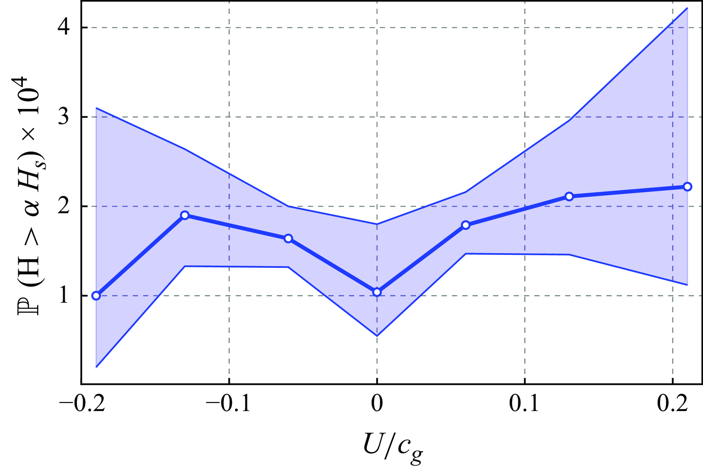
Figure 3. Exceedance probability of rogue waves ( $\alpha = 2.0$ ) in the southern North Sea with low-resolution binning of the normalised tidal current $U/c_{g}$ . The error band is computed from the 95 % Jeffreys confidence interval. The numbers of waves and rogue waves corresponding to each point are displayed in table 1.

Table 1. Numbers of waves and rogue waves associated with each point of figure 3.

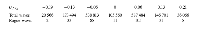
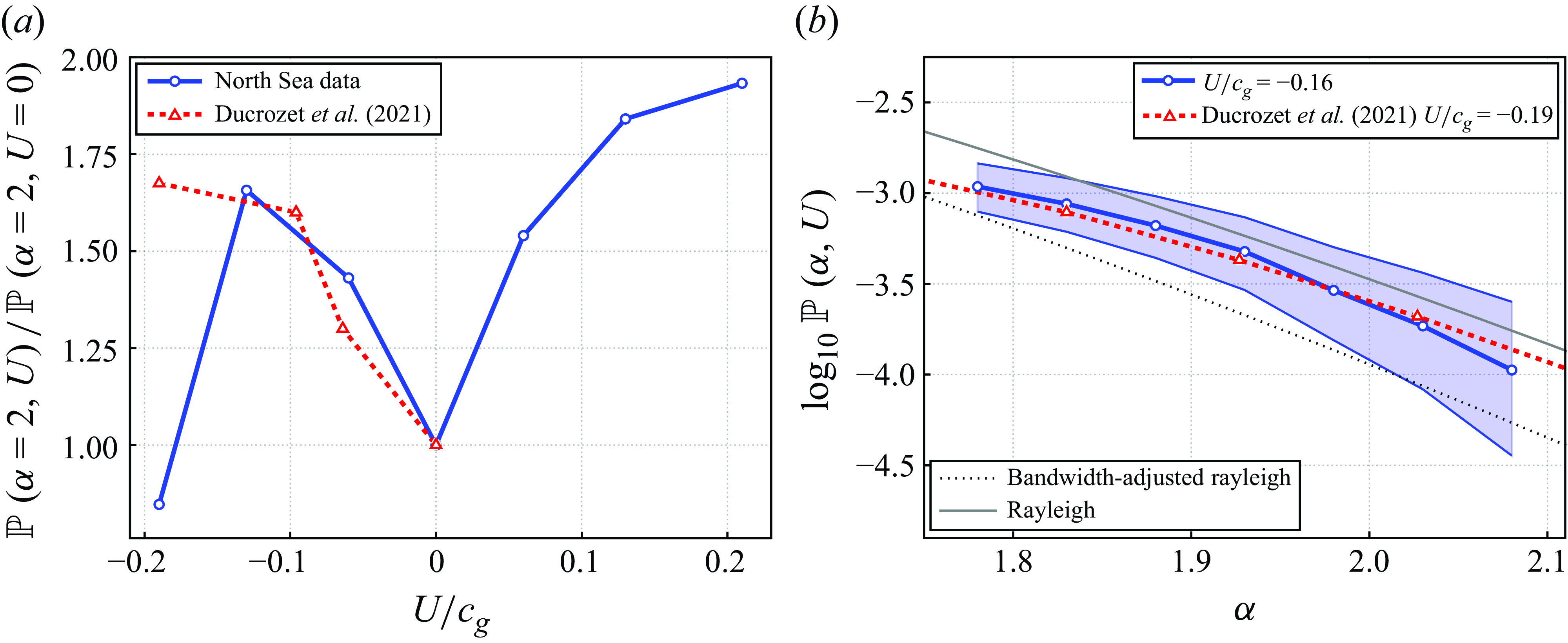
Figure 4. (a) Amplification of the observed rogue wave exceedance probability by opposing and following currents in comparison with laboratory measurements of Ducrozet et al. (2021), (3.1). Confidence intervals on observations are not shown as they are the same as in figure 3. (b) Exceedance probability for rest conditions as expected by Longuet-Higgins (1980) and for the bin of highest amplification ( $-0.12 \lt U/c_{{g}} \lt -0.16$ ), as a function of the threshold $\alpha$ .

Table 2. Hypergeometric $p$ -value calculated from the Fisher exact test for relevant pairs of data points of figure 3.

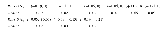
Figure 4 compares the rogue wave probability amplification observed in our data with Toffoli et al.’s (2015) experimental results, further described by Ducrozet et al. (2021), as a function of the relative velocity of the tidal current (panel a), and of the considered threshold $\alpha$ (panel b). The experiments are one-dimensional (1 + 1, unidimensional in space and time). In contrast, in our data, waves show a significant directional spread, introducing a second spatial dimension (2 + 1). Therefore, the exceedance probabilities in rest conditions are different, so that we compared the amplification ratios with regard to the latter

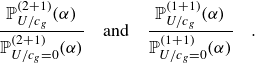(3.1) \begin{equation} \frac {\mathbb{P}_{U/c_g}^{(2+1)}(\alpha )}{\mathbb{P}_{U/c_g=0}^{(2+1)}(\alpha )} \quad \textrm {and} \quad \frac {\mathbb{P}_{U/c_g}^{(1+1)}(\alpha )}{\mathbb{P}_{U/c_g=0}^{(1+1)}(\alpha )} \quad . \end{equation}

The match between field observations and flume experiments is remarkable, especially when keeping in mind the wide range of conditions and the directional spread present in our dataset.

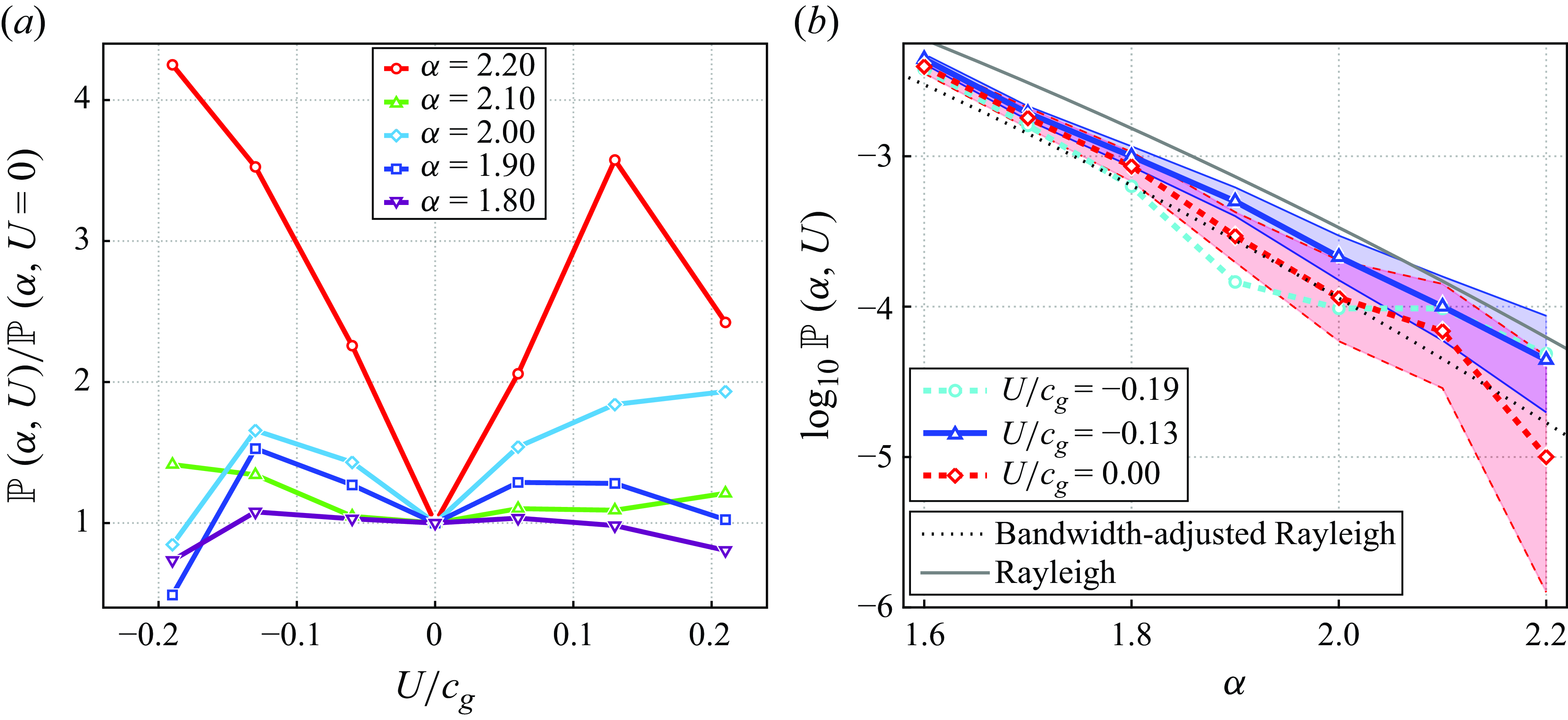
Figure 5. (a) Amplification of the exceedance probability of extreme waves as a function of the current velocity, for several values of the threshold $\alpha$ and (b) exceedance probability as a function of $\alpha$ for bins with rest conditions ( $U/c_g = 0$ ), maximal amplification ( $U/c_g = -0.13$ ) and of expected wave breaking conditions ( $U/c_g = -0.19$ ). To maximise legibility, confidence intervals in panel (a) observations are not shown, as panel (b) provides their magnitude for the rest conditions and the peak of the opposing current. Furthermore, the confidence intervals for $\alpha = 2.0$ are the same as in figure 3.

3.2. Influence of the threshold $\alpha$ on the exceedance probabilities

Hitherto, we have focused on the exceedance probability for a value of $\alpha = 2$ , corresponding to the common definition of rogue waves. As displayed in figure 5, the choice of $\alpha$ does not qualitatively impact our main finding, as long as $\alpha$ is sufficiently high. The difference between the rest and opposing current conditions is significant from a statistical point of view ( $p \lt 0.05$ , see table 3) for $1.7 \leqslant \alpha \leqslant 2.0$ . The ratio between the two curves of figure 5 begins to increase further for $\alpha \geqslant 1.9$ , which also corresponds to the regime in which amplification by following and opposing currents is observed, up to a normalised current speed $|U/c_g|\approx 0.13$ . In addition, we also compare it with the curve (cyan) for the bin with the highest values of the opposing current $|U/c_g|\approx 0.19$ where wave breaking is expected to appear. The amplification tends to increase for increasing values of $\alpha$ , where a smaller fraction of the wave height distribution is included, enhancing the weight of the tail of the probability distribution function. However, as the definition of extreme events becomes more stringent for higher $\alpha$ , such events become sparser, leading to the loss of statistical significance for $\alpha \geqslant 2.1$ .

Table 3. Hypergeometric $p$ -value calculated from Fisher’s exact test for differences between wave height exceedance probabilities at rest and in opposing current conditions (red and blue curves of figure 5 b).

3.3. Wave crest statistics

To check if our analysis is specific to wave height statistics, we performed the same work based on wave crest distributions (figure 6). In this case, the exceedance probability $\mathbb{P}(\beta , U)$ corresponds to crest heights $H_c$ exceeding $\beta H_s$ . The rest conditions and the bin that maximises the crest-to-trough height probability are compared with both the Rayleigh distribution for crests (Longuet-Higgins 1952) and its nonlinear counterpart (Tayfun 1980). The latter distribution is plotted for a steepness typical of the rest conditions ( $U/c_g = 0$ ) with $\varepsilon = 0.06$ . The wave crest corresponds to 55 %–65 % of the total wave height (Mendes et al. 2021). Thus, we expect similar behaviours for $\mathbb{P}(\beta , U)$ and $\mathbb{P}(\alpha , U)$ with $\beta \simeq 0.6 \alpha$ .

Indeed, the ratio between the exceedance probabilities of wave crests in rest and in opposing current conditions (figure 6) visually rises beyond $\beta = 0.6 \times 1.9 \simeq 1.15$ . The case $\alpha = 1.9$ corresponds to the point where the similar ratio for wave heights starts to increase (figure 5 b). However, the amplification of the exceedance probabilities for wave crests looses its statistical significance as compared with wave heights beyond $\beta = 1.7$ . This can be understood by considering that the Rayleigh distribution for wave crests evolves as

(3.2) \begin{equation} {\exp {(-8\beta ^2)} \approx \exp {(-2.9\alpha ^2)},} \end{equation}

as compared with $\exp {(-2\alpha ^2)}$ for wave heights (Longuet-Higgins 1952). This faster decay of the wave crest distribution results in sparser events, which undermine the statistical significance. Consequently, wave heights appear more relevant than wave crests for assessing heavy-tailed wave distributions.

We also note that the exceedance probabilities for both the rest and the opposing current conditions drastically deviate from the Rayleigh distribution up to a level similar to the nonlinear distribution introduced by Tayfun (1980). This deviation confirms the nonlinearity of the statistical distribution induced by currents, although it is more marked for wave crests than for wave heights.

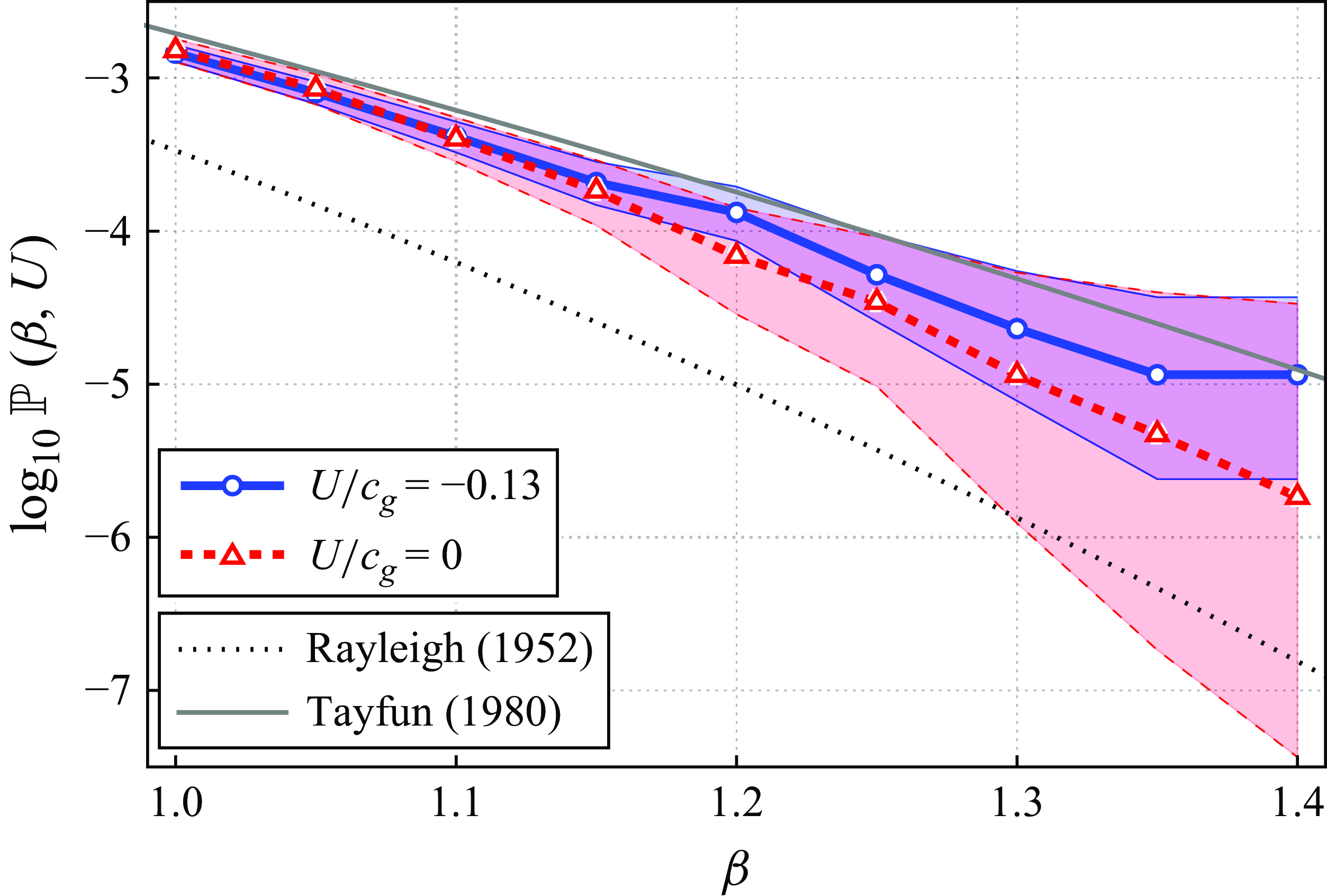
Figure 6. Exceedance probability of rogue wave crests ( $\beta = H_c/H_s$ ) for the entire North Sea data. The error band is computed from the 95 % Jeffreys confidence interval.

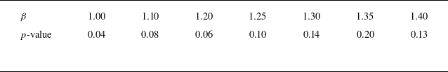
Table 4. Hypergeometric $p$ -value calculated from the Fisher exact test on the difference between wave crest height exceedance probabilities in rest and in opposing current conditions (red and blue curves of figure 6).

3.4. Influence of nonlinearity

We further investigate the behaviour in different ranges of wave steepness. Figure 7 displays the rogue wave amplification probability as a function of the current speed, for three ranges of steepness, corresponding to linear ( $\varepsilon \leqslant 0.05$ ), second-order ( $0.05 \leqslant \varepsilon \leqslant 0.9$ ) and higher-order ( $\varepsilon \geqslant 0.9$ ) regimes, respectively. The amplification of the rogue wave probability observed in figure 3 mainly originates from the second-order steepness range. In contrast, the amplification is weaker in the linear regime. More surprisingly, it vanishes in the higher-order regime. In the latter case, the onset of wave breaking associated with the large steepness likely levels off the wave height distribution, limiting the occurrence of rogue waves. Thus, the steepness regime is relevant for rogue wave occurrence.

3.5. Robustness assessment: definition of depth and rest conditions

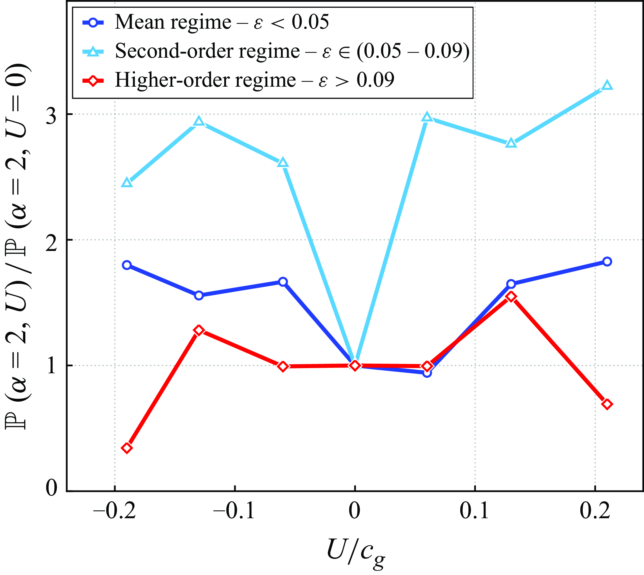
Figure 7. Effect of steepness on the rogue wave amplification by tidal currents for different linearity ranges.

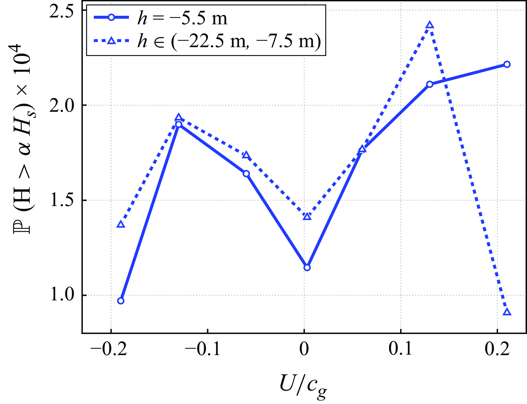
Figure 8. Exceedance probability $P_\alpha$ for $\alpha = 2.0$ as a function of the normalised current velocity $U/c_g$ measured at $h=-5.5$ m and taken as an average in the range $-22.5\,\textrm {m} \lt h \lt -7.5\,\textrm {m}$ . Confidence intervals are not shown since they are the same as in figure 3.

As mentioned in § 2, the water depth at the measurement location (30 m) is sufficiently small compared with the wavelength ( $\sim$ 100 m) for the waves to be influenced by the current over the full water column. We checked that our results are robust against the choice of the depth at which the current speed was measured, by comparing our results obtained by considering the current at $h=-5.5$ m with those obtained by considering $U/c_g$ averaged between $h = -7.5$ and $-22.5$ m. The behaviours are comparable, except in the rightmost bin corresponding to a fast following current (figure 8). However, as discussed above, the extremely large confidence interval on this bin limits the relevance of these differences. A similar check was performed by considering the current at $h = -15$ m (not shown), leading to the same conclusion. This relative independence of our results of the depth at which the current speed was measured, facilitates the comparison with experiments, where the vertical current profile is generally homogeneous (Ducrozet et al. 2021; Zhang et al. 2023). Finally, figure 9 displays the rogue wave amplification of probability for three definitions of the boundaries of the central bin, i.e. the rest condition. Obviously, the impact of this choice on our results is minimal, especially when comparing the differences between the curves with the typical width of the confidence interval of the data (see figure 3).

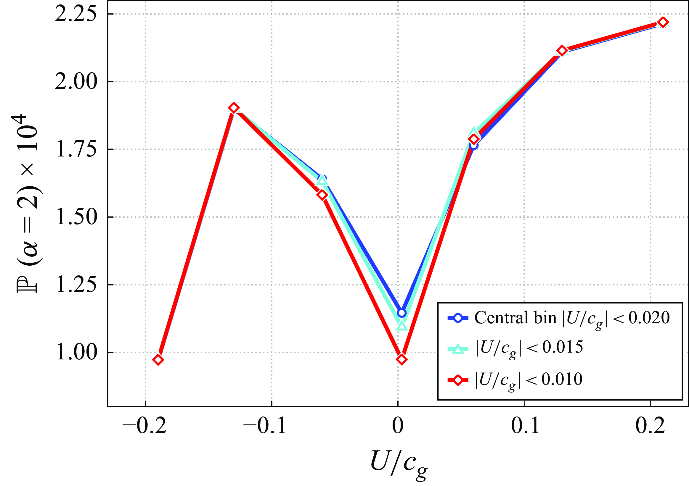
Figure 9. Sensitivity to different definitions of the rest condition (legend) of the exceedance probability of rogue waves ( $\alpha = 2$ ). Confidence intervals are not shown since they are the same as in figure 3.

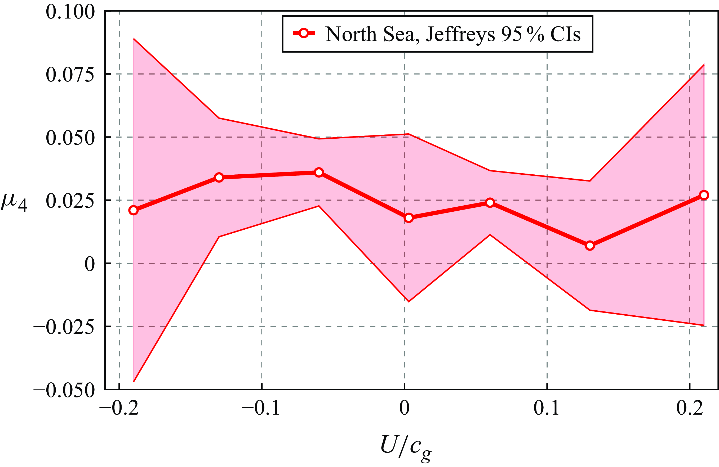
Figure 10. Estimated mean excess kurtosis and its 95% confidencen intervals as a function of the tidal current.

3.6. Alternative metrics of enhanced rogue wave activity

The excess kurtosis is widely used as a proxy for measuring the degree of nonlinearity of ocean waves (Longuet-Higgins 1963; Marthinsen 1992; Mori & Janssen 2006). Figure 10 displays the average excess kurtosis for each tidal velocity bin. The variations with the current are well below statistical significance (table 5). This can be understood by considering that excess kurtosis holds as a proxy of the wave nonlinearity only if the initially linear waves have a quasi-Gaussian distribution of the surface elevation (Longuet-Higgins 1952). While this is the case in laboratory-controlled experiments (Zhang et al. 2019; Li et al. 2021), it is less trustworthy in real-ocean observations (Stansell 2004; Christou & Ewans 2014; Cattrell et al. 2018). The rest condition data of figure 5(b) illustrate the empirical sub-Gaussian exceedance probability at rest conditions $(U/c_g =0)$ . This dependence is well fitted by (Longuet-Higgins 1980; Mendes & Scotti 2020)

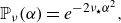(3.3) \begin{equation} {\mathbb{P}_{\nu }(\alpha ) = e^{-2\nu _{\star }\alpha ^{2}},} \end{equation}

where

Table 5. Hypergeometric $p$ -value calculated from the Fisher exact test for selected pairs of data points of figure 10.

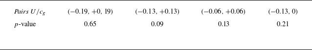
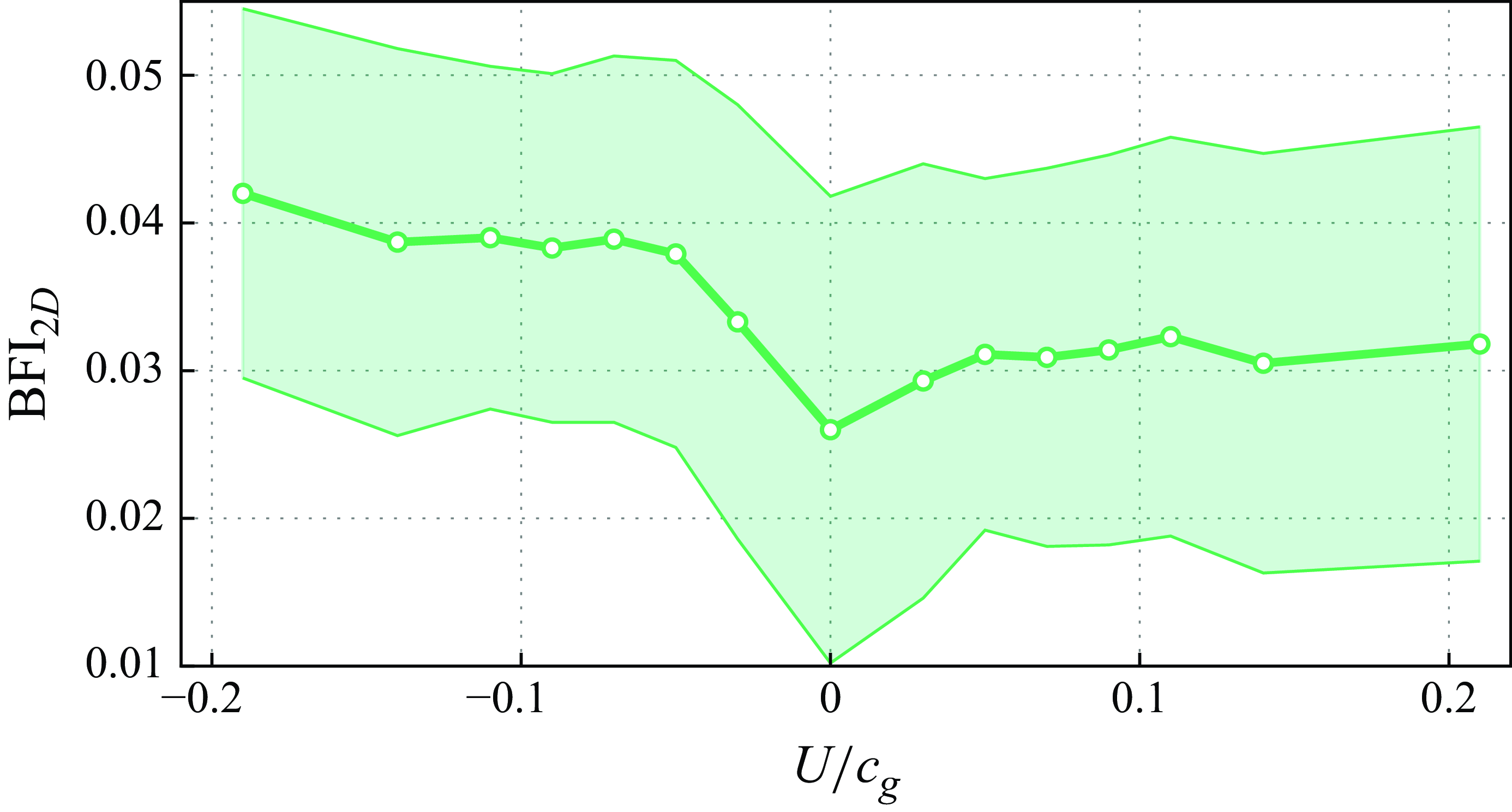
Figure 11. Response of the mean directional Benjamin–Feir index ( $\textit{BFI}_{2D}$ ), as computed from (37) of Mori et al. (2011), to the normalised tidal intensity. Error bands display data with plus or minus one standard deviation.

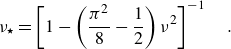(3.4) \begin{equation} {\nu _{\star } = \left [ 1 - \left ( \frac {\pi ^2}{8} - \frac {1}{2} \right ) \nu ^{2} \right ]^{-1} \quad .} \end{equation}

This sub-Gaussian probability is likely due to the broadbanded spectrum in the North Sea data. If we use a Gram–Charlier expansion for the exceedance probability of the type $1 + ({\mu _{4}}/{2}) \alpha ^{2} ( \alpha ^{2} - 1 )$ for the ratio between non-Gaussian and Gaussian distributions (Mori & Yasuda 2002), comparison with the broadbanded distribution of (3.3) leads to $\mu _4 \approx ( 1 - \pi ^2/4 ) 2\nu ^{2}/(\alpha ^{2} - 1) \sim - \nu ^{2}$ . As such, the reference kurtosis in rest conditions is sub-Gaussian (negative). Consequently, a threefold increase in the probability of exceedance with such rest conditions will increase the kurtosis by small fractions ( ${\lesssim}1/10$ ). In contrast, if the rest conditions had $\mu _4 = 0$ , its increase would be ${\gtrsim}1/3$ . This kurtosis reference bias weakens the kurtosis as a relevant metric in the conditions of our open sea data.

Table 6. Hypergeometric $p$ -value calculated from the Fisher exact test for selected pairs of data points of figure 11. $p$ -values are very small in all cases, ergo we also highlight their $\chi ^2$ values in italics to allow for comparison.

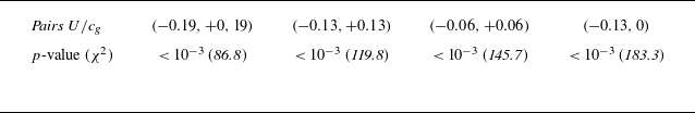
Finally, BFI is also generally considered as a key indicator of the ability of rogue waves to develop and grow (Mori & Janssen 2006; Mori et al. 2011). Its dependency on the tidal current relative to the wave direction (figure 11) displays a significant asymmetry between opposing and following currents (table 6). However, as also evidenced in figure 2(f), the values of the BFI are well below the value of $0.3$ that would be required for it to initiate the development of rogue waves.

4. Discussion

The most striking result from our observations is that both following and opposing currents amplify the rogue wave probability, compared with rest conditions. While the results regarding opposing currents are consistent with previous wave tank experiments (Toffoli et al. 2015; Ducrozet et al. 2021), those regarding following currents are unexpected. Therefore, in this section we discuss the physical mechanisms that may explain them.

First, let us note that the symmetrical behaviour cannot be explained by the recently reported symmetric rise of the wave height with stronger currents (Teutsch et al. 2024), because the rogue wave probability does not depend on $H_s$ (Stansell 2004; Christou & Ewans 2014; Mendes et al. 2021). The strong reported increase in the relative water depth $k_ph$ for $|U/c_g| \gt 0.1$ as compared with rest conditions (Teutsch et al. 2024) cannot affect the wave statistics either, because the wave field is already in the deep water regime (figure 2 b). This absence of the effect is well described by a spectral analysis of out-of-equilibrium systems (Mendes et al. 2022; Mendes & Kasparian 2022, 2023).

The steepness also increases, as compared with rest conditions, for both directions of current, but significantly more for an opposing one (see figure 2a and figures 5a and 6a of Teutsch et al. 2024). The steepness growth is expected to translate into an increase of the exceedance probability (Tayfun 1980; Mendes et al. 2022; Mendes & Kasparian 2022, 2023). However, the asymmetry of the steepness growth prevents it from being the dominant driver of the symmetric increase of the exceedance probability.

As compared with the rest condition, currents increase the directional spread (figure 6f in Teutsch et al. 2024) and decrease the bandwidth (figure 6e in Teutsch et al. 2024). These dependencies, which are more marked for ( $U/c_g \geqslant 0.08$ ), i.e. beyond the peaks of panels c and d of figure 2, should respectively decrease (Mori et al. 2011; Lyu, Mori & Kashima 2023) and increase (Longuet-Higgins 1980) the rogue wave probability, so that their effects likely compensate each other.

Finally, likely due to large directional spread and bandwidth , the Benjamin–Feir index is limited to values insufficient to induce the large observed exceedance probability amplification $(\textit{BFI} \lt 0.05 \propto \varepsilon / \nu )$ . Thus, the BFI cannot help to interpret the magnitude of the amplification, nor contradict the symmetry between forward and opposing currents.

The remaining variable capable of leading the rogue wave amplification is therefore the relative current speed $U/c_{g}$ itself. It was already pointed out theoretically by Toffoli et al. (2010, 2015) from the perspective of the NLSE framework that maximum amplitudes of regular waves should depend on $U/c_{g}$ . Mendes & Kasparian (2022) have theoretically shown that the set down of waves travelling past a shoal mostly controls the magnitude of the anomalous statistics. Laboratory experiments have demonstrated small changes in the wave-driven set down due to wave–current interaction (Svendsen & Hansen 1986; Jonsson 2005), but stronger ones for the effect of tides over reefs (Becker, Merrifield & Ford 2014; Yao et al. 2020, 2023). The same should also apply in the open sea over flat bottoms. Indeed, the wave-driven set down is negligible in deep water (Longuet-Higgins & Stewart 1962), while the set down due to wave–current interaction in deep water is proportional to the ratio $-U^{2}/2g$ , which can be rewritten in terms of $-(U/c_{g})^{2}/8k$ (Brevik 1978; Jonsson 1978). This quadratic dependence on current velocity, hence on the associated set down, may explain the observed symmetry of extreme wave statistic amplification, and especially the amplification of rogue wave occurrence probability by following currents.

Our finding regarding the similar effects of opposing and following currents of the same speed on rogue wave probability also recalls the results of Waseda et al. (2015), who have shown that the effect of currents on resonant interactions is symmetrical, although the main driving parameter was the current gradient. Investigating this aspect would, however, require long-term series from several locations, which is clearly out of the scope of the present data and the analysis thereof.

Furthermore, the tidal current oscillates with a period of approximately 12 h. Investigating the influence of this slight non-stationarity, as well as of spatial inhomogeneities on the extreme wave statistics (Ho et al. 2023; Halsne et al. 2024) would provide further refinement of the comparison with flume experiments (Toffoli et al. 2010,2013; Waseda et al. 2015; Ducrozet et al. 2021).

Comparing several alternative indicators, we find that the wave height is the most suitable variable to investigate the tail of wave distributions. In comparison, wave crests provide more sparse data at the upper end of the probability distribution, reducing the statistical significance. This is likely due to the wave asymmetry between crests and troughs. This asymmetry affects the tail of the statistics such that the empirical ratio of 0.6 between $\beta$ and $\alpha$ does not allow a direct correspondence between the two distributions. From a mathematical point of view, this discrepancy stems from the different decay rates of the distribution tails, as illustrated by (3.2) (Mendes et al. 2021).

Finally, we have found that the excess kurtosis fails as a proxy when the initial distributions are too far from normal, while the effect of the BFI in typical marine conditions is insufficient to drive the formation of rogue waves, reducing its relevance in that case.

5. Conclusion

In this work, we present the first long-term observational statistical study of the effect of both following and opposing currents on rogue wave statistics, based on data of wave–tide interaction. Following currents amplify rogue wave occurrence as much as opposing currents. The amplification rises at least up to $U/c_g \approx \pm 0.13$ . Therefore, not only waves travelling against large ocean currents such as the Gulf or Agulhas Stream are prone to rogue wave formation, but also waves interacting with tidal streams. This finding sheds light on a widely distributed type of risk. While strong wide streams are not that common, tidal currents are found on nearly every coast.

Moreover, subsets of the dataset with different ranges of steepness display the same symmetry, but feature different magnitudes: second-order seas imply the highest amplification, followed by steep seas near breaking conditions, while linear seas have the lowest amplification magnitude.

Although our results are comparable to experimental observations in unidimensional irregular wave fields interacting with stationary opposing currents, this similarity is striking, since our data are broadbanded and show a substantial directional spread, which are both known to weaken rogue wave occurrence (Longuet-Higgins 1980; Karmpadakis, Swan & Christou 2022). Systematic wave tank studies with a better control of the conditions would be necessary to provide a clearer conclusion. An extensive investigation of the effect of narrowing the ranges of steepness and directional spread would also be highly valuable. Indeed, we analysed more homogeneous data subsets and found indications (although not statistically significant and therefore not shown) that data homogeneity may result in a much stronger amplification by the current.