Uniform bounds for polynomial Carleson operators and oscillatory integrals of Radon type

Abstract

In this paper, we establish the $L^p$ bounds for partial polynomial Carleson operators along polynomial curves for $p \gt 1$, which depend only on $p$ and the number of monomials in the defining polynomial. Additionally, we study two classes of oscillatory integral operators of Radon type and derive uniform $L^2$ bounds.

1. Introduction

1.1. Classical Carleson operator

For $f \in \mathcal{S}(\mathbb{R})$, the classical Carleson operator is defined as

\begin{equation*}f(x)\longmapsto\sup_{N\in \mathbb{R}}\bigg \vert {p.v.} \int _{\mathbb{R}} f(x-t) e^{iNt}\frac{dt}{t} \bigg\vert, \end{equation*}

where p.v. denotes the Cauchy principal value. This operator was introduced by Carleson [6] in the study of the convergence properties of Fourier series. Historically, this problem traces back to Lusin’s conjecture, which asserts that the Fourier series of any function in $ L^2(\mathbb{T}) $ converges almost everywhere when $\mathbb{T}=[0,2\pi]$. A significant obstacle to this conjecture was Kolmogorov’s counterexample [14, 15], which demonstrated that there exist functions in $ L^1(\mathbb{T}) $ whose Fourier series diverge almost everywhere. This result led to a long-standing misconception that Fourier series might generally exhibit poor convergence properties.

After decades of misapprehension in light of Kolmogorov’s result, Carleson [6] proved that Lusin’s conjecture is true by establishing the $ L^2 $ to $ L^{2, \infty} $ boundedness of the Carleson operator, thereby establishing the almost everywhere convergence of Fourier series for functions in $ L^2(\mathbb{T}) $. More precisely, he showed that for $ f \in L^2(\mathbb{T}) $, the sequence of partial Fourier sums

\begin{equation*} s_n f (x) = \sum_{|k| \leq n} \hat{f}(k) e^{ikx} \end{equation*}

converges almost everywhere. In his proof, Carleson studied an operator of the form

\begin{equation*} \int _{-4\pi}^{4\pi} f(t)e^{int}\frac{1}{x-t}dt, \end{equation*}

whose boundedness played a crucial role in establishing his result. Later on, Hunt [13] extended Carleson’s theorem to $ L^p(\mathbb{T}) $ spaces for $ 1 \lt p \lt \infty $. This generalization significantly broadened the applicability of Carleson’s techniques beyond the Hilbert space setting. Further progress was made by Sjölin [27] who considered the $ L^p $ boundedness of the higher-dimensional Carleson operator

\begin{equation*}f(x)\longmapsto\sup _{N\in \mathbb{R}^s}\bigg \vert {p.v.} \int _{\mathbb{T}^s} f(x-t) e^{iNt}\frac{dt}{t} \bigg\vert, \end{equation*}

where $ \mathbb{T}^s $ denotes the $ s $-dimensional torus. Subsequently, Fefferman [7] provided an alternative proof of the Carleson–Hunt Theorem, which was conceptually simpler and laid the foundation for the modern time-frequency analysis framework. Lacey and Thiele also [18] developed a simple proof for the Carleson–Hunt Theorem by employing time-frequency analysis and techniques from the study of the bilinear Hilbert transform. Notably, significant progress has been made in the study of the bilinear Hilbert transform, including the celebrated works of Lacey and Thiele [16, 17], Grafakos and Li [9], and Li and Xiao [19].

1.2. Polynomial Carleson operators

Beyond the bilinear Hilbert transform, considerable attention has been devoted to the study of general Calderón–Zygmund operators that extend beyond the Hilbert kernel. For more details, we refer the readers to the works of Sjölin [27, 28], Stein [31], and the references therein.

In [31], Stein considered the following polynomial Carleson operator

(1.1)\begin{equation} f(x) \mapsto \sup_P \left| \int_{\mathbb{R}^n} f(x - t) e^{iP(t)} K(t) \, dt \right|, \end{equation}

where $ K $ is a suitable Calderón–Zygmund kernel and the supremum is taken over all real-valued polynomials $ P $ of degree at most $ d $ in $ n $ variables. For example, one may consider the kernel $K$ as a tempered distribution that agrees with a $C^1$ function $K(x)$ for $x\neq 0$, such that $\vert \partial ^{\alpha}_{x}K(x)\vert \ll \vert x \vert ^{-n-\vert \alpha\vert}$ for $ 0\leq \vert \alpha\vert \leq 1$, and $\hat{K}\in L^{\infty}$.

Stein’s investigation centred on the question of whether the polynomial Carleson operator is bounded on $ L^p $ for $ 1 \lt p \lt \infty $. When $ d = 1 $, the problem reduces to the classical Carleson case, corresponding to the zero-curvature scenario. However, when $ d \geq 2 $, it corresponds to the non-zero curvature case. Specifically, for $ d = 2 $ and $n=1$, Stein [31] first established the $ L^2(\mathbb{R}) $-boundedness of the polynomial Carleson operator. For $ d \geq 2 $, Stein and Wainger [33] proved that if the polynomial $ P $ is restricted to the class of polynomials of degree at most $ d $ such that $ P(0) = P'(0) = 0 $, then the operator is bounded on $ L^p(\mathbb{R}^n) $ for $ 1 \lt p \lt \infty $. In the case $ n = 1 $, Lie [20, 22] showed the $ L^p $-boundedness of the polynomial Carleson operator without any restrictions on $ P $. In the general case of $d\geq 2$, Lie [21] and Zorin-Kranich [34] proved that the polynomial Carleson operator is bounded on $ L^p(\mathbb{R}^n) $ for any $ p \gt 1 $ when the kernel $K$ enjoys certain Hölder continuous kernel conditions.

Consider now the Carleson operator in the special case $K(t)=1/t$. In 2017, Guo, Hickman, Lie, and Roos [11] considered the operator in (1.1) for $P(t)=Nt + M [t]^{\alpha}$, namely

\begin{equation*} f(x) \mapsto \sup_{N,M \in \mathbb{R}} \left| {p.v.}\int_{\mathbb{R}} f(x - t) e^{iNt + iM [t]^{\alpha}} \frac{dt}{t} \right|, \end{equation*}

where $ [t]^{\alpha} $ denotes either $ \text{sign}(t) |t|^{\alpha} $ or $ |t|^{\alpha} $. They demonstrated that this operator is bounded on $ L^p $ for $ \alpha \in \mathbb{R} $ and $ \alpha \notin \{0, 1\} $. On the other hand, it was Ramos [25] who investigated the uniform $ L^p $-boundedness for the operator

\begin{equation*} f(x) \mapsto \sup_{N \in \mathbb{R}} \left|{p.v.} \int_{\mathbb{R}} f(x - t) e^{iNt + iP(t)} \frac{dt}{t} \right|. \end{equation*}

The main result in [25] is as follows:

Theorem A ([25])

Let $P$ be a polynomial, $P(t)=a_1 t^{\alpha _1} + \cdots + a_d t^{\alpha _d}$ with $d \in \mathbb{N}$, $a_i \in \mathbb{R}$, $1 \lt \alpha _i \in \mathbb{Z}_{+}$ $(1\leqslant i\leqslant d)$, $deg P=\max _{1\leqslant i \leqslant d}\lbrace \alpha_{i}\rbrace$, and $1 \lt p \lt \infty$, then we have

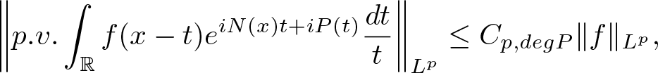(1.2)\begin{equation} \bigg\Vert {p.v.}\int_{\mathbb{R}} f(x-t)e^{iN(x)t+iP(t)}\frac{dt}{t}\bigg\Vert_{L^p}\leq C_{p,deg P}\Vert f\Vert_{L^p}, \end{equation}

where $C_{p,deq P}$ is a constant that depends only on $p$ and $deg P$. Furthermore,

(1.3)\begin{equation} \bigg\Vert \sup_{N\in \mathbb{R}}\bigg\vert {p.v.} \int_{\mathbb{R}} f(x-t)e^{iNt+iP(t)}\frac{dt}{t}\bigg \vert\bigg\Vert_{L^p}\leq C_{p,deg P}\Vert f\Vert_{L^p}. \end{equation}

Remark 1.1. The constant $ C_{p, \deg P} $ in inequalities (1.2) and (1.3) can be refined to a constant $ C_{p, d} $, where $ d $ denotes the number of monomials in the polynomial $P$. This improvement follows from a minor refinement in the choice of the large constant in the gap decomposition, as described in [25]. Specifically, by adjusting this choice to depend solely on $ d $ rather than on $ \deg P $, both in the decomposition and in handling the contribution for bad scales, the dependence on the polynomial’s degree can be eliminated.

1.3. Polynomial Carleson operators of Radon type

In recent years, significant progress has been made in the study of polynomial Carleson operators of the form (1.1) along various classes of curves (Radon-type). Let

(1.4)\begin{equation} Rf(x)= \int_{\mathbb{R}^n} f(x-\gamma (t))e^{iP(t)}K(t)dt , \end{equation}

where $\gamma$ is a function defined on $\mathbb{R}^n$ whose image is an $n$-dimensional submanifold of $\mathbb{R}^m$ of finite type, $K$ is a suitable Calderón–Zygmund kernel and $P$ is real-valued polynomial in $n$ variables. The corresponding maximally modulated Carleson operator of Radon type is defined by

(1.5)\begin{equation}Cf(x)= \sup_{P\in \mathcal{P}}\bigg \vert \int_{\mathbb{R}^n} f(x-\gamma (t))e^{iP(t)}K(t)dt \bigg \vert,\end{equation}

where $\mathcal{P}$ is a chosen class of polynomials.

A natural question that arises in this context is whether the polynomial Carlson operator of Radon type is bounded on $ L^p $ for $ 1 \lt p \lt \infty $. It was Pierce and Yung [23] who initiated the study of the case where the defining curve is the paraboloid $ \gamma(t) = (t, |t|^2) $. Specifically, they considered the operator

\begin{equation*} f(x,y) \longmapsto \sup_{P \in \mathcal{P}} \left| \int_{\mathbb{R}^n} f(x - t, y - |t|^2) e^{i P(t)} K(t) \, dt \right|, \end{equation*}

where $ K $ is a suitable Calderón–Zygmund kernel, and $ \mathcal{P} $ is a finite-dimensional subspace of polynomials of degree at most $ d $. Pierce and Yung established $ L^p $ boundedness for certain subspaces $ \mathcal{P} $ that exclude linear and specific quadratic terms in dimensions $ n \geq 2 $. The case $ n=1 $, corresponding to the planar setting, was later studied by Guo, Pierce, Roos, and Yung [12], who considered a weaker formulation of the problem. When $K(t)={1}/{t}$, the authors in [12] obtained the $ L^p $ $ (1 \lt p \lt \infty) $ boundedness of the following two polynomial Carlson operators along the curve $(t,t^m)$:

\begin{equation*}A_{N}^{m,d}f(x,y)=p.v. \int _{\mathbb{R}} f(x-t, y-t^m) e^{iN(x)t^d}\frac{dt}{t}\end{equation*}

and

\begin{equation*}B_{N}^{m,d}f(x,y)=p.v. \int _{\mathbb{R}} f(x-t, y-t^m) e^{iN(y)t^d}\frac{dt}{t},\end{equation*}

where $ N $ is a measurable function defined on $\mathbb{R}$. Their results, in turn, yield that

• • $ \bigg\Vert\sup_{N\in \mathbb{R}} \bigg \Vert p.v.\int_{\mathbb{R}} f(x-t, y-t ^m)e^{iNt^d}\frac{dt}{t} \bigg \Vert_{L^p(dy)}\bigg\Vert_{L^p(dx)}\lesssim \Vert f\Vert _{L^p}, \text{for }$ $1 \lt p \lt \infty.$ where $d=1$, $m\geq 3$ or $d$, $m \gt 1$, $d\neq m$; and

• • $ \bigg\Vert\sup_{N\in \mathbb{R}} \bigg \Vert p.v.\int_{\mathbb{R}} f(x-t, y-t ^m)e^{iNt^d}\frac{dt}{t} \bigg \Vert_{L^p(dx)}\bigg\Vert_{L^p(dy)}\lesssim \Vert f\Vert _{L^p}, \text{for }$ $1 \lt p \lt \infty.$ where $d=m\geq 2$ or $d$, $m \gt 1$, $d\neq m$.

Recently, Roos [26], Ramos [24], and Becker [2, 3] studied the boundedness of planar Pierce-Yung operators by analyzing them within the framework of modulation-invariant operators. In a related direction, when kernel $K(t) ={1}/{t}, $ Beltran, Guo, and Hickman [4] established the $ L^p $ bounds for the Radon-type Carleson operator $ C $ in (1.5) associated with the mapping

\begin{equation*} \gamma(t) = (t, t^2), \quad P(t) = v t^3, \quad v \in \mathbb{R}. \end{equation*}

They also pointed out that their method can be applied to operators with more general Calderón–Zygmund kernels.

This paper aims to study the uniform bounds problem for the polynomial Carleson operators of Radon type. We begin by introducing some notions and definitions. Let $ f $ be a Schwartz function on $ \mathbb{R}^2 $ and define the Carleson operator $ R $ associated with polynomial curves $ (t, P(t))_{t \in \mathbb{R}} $ by

\begin{equation*} \mathcal {R}f(x,y)=\mathcal{C}_{N}^{P,m}f(x,y)=p.v.\int _{\mathbb{R}}f(x-t,y-P(t))e^{iNt^m}\frac{dt}{t}, \end{equation*}

where $ N \in \mathbb{R} $, $ m $ is a positive integer, and $ P(t) $ is a polynomial of the form $P(t)=a_1 t^{\alpha _1} + \cdots + a_d t^{\alpha _d}$ with $d \in \mathbb{N}$, $a_i \in \mathbb{R}$ and $2 \lt \alpha _i \in \mathbb{Z}_{+}$ $(1\leqslant i\leqslant d)$.

Motivated by the work of [12], in this paper, we first consider the uniform bounds of the operator $A_N ^{P,1}$ defined by

\begin{equation*} A_N^{P,1}f(x,y):=\mathcal{C}_{N(x)}^{P,1}f(x,y), \end{equation*}

where $N(x)$ is a measurable function defined on $\mathbb R.$

Our first main result of this paper is as follows:

Theorem 1.2. Given $d \in \mathbb{N}$, for every $1 \lt p \lt \infty$, we have

(1.6)\begin{equation} \Vert A_N ^{P,1} f\Vert _{L^p} \leq C_{p,d} \Vert f \Vert _{L^p}, \end{equation}

and

(1.7)\begin{equation} \Vert \sup _{N\in \mathbb{R}}\Vert \mathcal{C}_N ^{P,1} f\Vert _{L^p(dy)}\Vert_{L^p(dx)} \leq C_{p,d} \Vert f \Vert _{L^p}. \end{equation}

where $ C_{p,d} $ is a constant depending only on $ d $ and $ p $, but independent of $ N $, $ a_i $, and $ \alpha_i $.

We note that the assumption that the minimal monomial of the polynomial has degree at least 3 is essential for the method used in this paper to apply TT* method in the high-frequency analysis. So we restrict attention to polynomials whose minimal monomial has degree at least 3.

Consider now the problem of obtaining uniform bounds for certain oscillatory integral operators. In [32], Stein and Wainger proved that

(1.8)\begin{equation} \bigg\Vert p.v.\int_{\mathbb{R}} f(x-t)e^{iP(t)}\frac{dt}{t}\bigg\Vert_{L^2}\leq C_{\alpha_i,d}\Vert f\Vert_{L^2}. \end{equation}

Guo[10] improved the estimate (1.8) to a uniform bound constant $C_d$ which is independent of $\alpha_i$.

Theorem B ([10])

Given $d \in \mathbb{N}$, we have

\begin{equation*} \bigg\Vert p.v.\int _{\mathbb{R}}f(x-t)e^{iP(t)}\frac{dt}{t}\bigg\Vert _{L^2} \leq C_{d} \Vert f \Vert _{L^2}. \end{equation*}

where $C_{d}$ is a constant that depends only on $d$, but not on any $a_i$ or $\alpha _i$.

Our second main purpose of this paper is to study the uniform estimates for the oscillatory integral operator of Radon type in (1.4) on $\mathbb{R}^2$. We consider two types of oscillatory integral operators as follows:

\begin{equation*}\mathcal{E}f(x,y)=p.v. \int_{\mathbb{R}} f(x-t,y-v(x)t-P(t))e^{iP(t)}\frac{dt}{t};\end{equation*}

and

\begin{equation*}Tf(x,y)=p.v. \int_{\mathbb{R}} f(x-t,y-v(x)t^2)e^{iP(t)}\frac{dt}{t}.\end{equation*}

We now summarize our results in the following theorems.

Theorem 1.3. Given $d \in \mathbb{N}$, we have

\begin{equation*} \Vert \mathcal{E} f\Vert _{L^2} \leq C_{d} \Vert f \Vert _{L^2}, \end{equation*}

where $C_{d}$ is a constant that depends only on $d$.

Theorem 1.4. Given $d \in \mathbb{N}$, we have

\begin{equation*} \Vert T f\Vert _{L^2} \leq C_{d} \Vert f \Vert _{L^2}, \end{equation*}

where $C_{d}$ is a constant that depends only on $d$.

Remark 1.5. As noted in Remark 1.1, Theorem 1.3 is not new. Although the exact statement does not appear explicitly in [25], it follows immediately via applying the Fourier transform in the second variable, Plancherel’s theorem, and refining their argument as described in Remark 1.1. However, we provide a new proof that may offer insights for extending the result to higher-dimensional cases. Theorem 1.4 also indicates that

\begin{equation*}\bigg\Vert p.v.\int_{\mathbb{R}} f(x-t)e^{iv(x)t^2+iP(t)}\frac{dt}{t}\bigg\Vert_{L^2}\leq C_{p,d}\Vert f\Vert_{L^2},\end{equation*}

which can be seen as a different case from the curve $(t, v(x)t)$ considered in [25].

The organization of this paper is as follows. In Section 2, we introduce some notations and some lemmas which will be used later. Sections 3–5 will be devoted to give the proofs of Theorem 1.2-1.4, respectively. Throughout this paper, we use $ C \gt 0 $ to denote a constant that may vary from line to line. We write $ A \lesssim B $ to indicate that $ A \leq C B $ for some absolute constant $ C $. If $ C $ depends on a parameter $ p $, we write $ A \lesssim_p B $ or equivalently $ A \leq C_p B $.

2. Preliminaries

Our main results in this paper rely on the Littlewood–Paley projection, making it necessary to establish certain vector-valued inequalities. In this section, we first present some fundamental results concerning these inequalities. Note that the maximally truncated Carleson operator is defined as

\begin{equation*} \mathcal{C}^*f(x)=\sup_{N\in \mathbb{R}, \varepsilon \gt 0} \bigg\vert p.v. \int_{\vert t\vert \leq \varepsilon}f(x-t)e^{iNt}\frac{dt}{t} \bigg\vert \end{equation*}

It is well known that the maximally truncated Carleson operator is bounded on $ L^p $. Here, what we need is the following vector-valued inequality for the maximally truncated Carleson operator.

Lemma 2.1. ([12])

For $1 \lt p \lt \infty$ and $i=1$, $2$, we have

\begin{equation*} \bigg\Vert \left( \sum_{k\in \mathbb{Z}}\vert\mathcal{C}^* f_k\vert ^2\right)^{\frac{1}{2}}\bigg\Vert_{L^p}\leq C_p \bigg\Vert \left( \sum_{k\in \mathbb{Z}} \vert f_k\vert ^2\right)^{\frac{1}{2}}\bigg\Vert_{L^p} \end{equation*}

where $C_{p}$ is a constant that depends only on $p$.

The relevant results are presented in Grafakos’ book ([8], Chapter 6) and are further compiled by the authors in [12].

The one-variable Hardy–Littlewood maximal functions in the plane, denoted by $ M_1 $ and $ M_2 $, are defined as

\begin{align*} M_1f(x,y)=\sup _{r \gt 0} \frac{1}{2r}\int_{-r}^r \vert f(x-u, y)\vert du; \end{align*}

\begin{align*} M_2f(x,y)=\sup _{r \gt 0} \frac{1}{2r}\int_{-r}^r \vert f(x, y-t)\vert dt. \end{align*}

Here, $ M_1 $ and $ M_2 $ correspond to the Hardy–Littlewood maximal functions applied in the horizontal and vertical directions, respectively. They are bounded on $L^p (\mathbb{R}^2)$ $1 \lt p \lt \infty$ and satisfy the following vector-valued inequality.

Lemma 2.2. ([30])

For $1 \lt p \lt \infty$ and $i=1$, $2$, we have

\begin{equation*} \bigg\Vert \left( \sum_{k\in \mathbb{Z}}\vert M_i f_k\vert ^2\right)^{\frac{1}{2}}\bigg\Vert_{L^p}\leq C_p \bigg\Vert \left( \sum_{k\in \mathbb{Z}} \vert f_k\vert ^2\right)^{\frac{1}{2}}\bigg\Vert_{L^p} \end{equation*}

where $C_{p}$ is a constant that depends only on $p$.

Consider now the maximal operator along curve $(t, P(t))$ defined by

\begin{align*} Mf(x,y)=\sup _{r \gt 0} \frac{1}{2r}\int_{-r}^r \vert f(x-t, y-P(t))\vert dt. \end{align*}

It enjoys the following property:

Lemma 2.3. ([29])

For $1 \lt p \lt \infty$, we have

\begin{equation*} \bigg\Vert \left( \sum_{k\in \mathbb{Z}}\vert M f_k\vert ^2\right)^{\frac{1}{2}}\bigg\Vert_{L^p}\leq C_p \bigg\Vert \left( \sum_{k\in \mathbb{Z}} \vert f_k\vert ^2\right)^{\frac{1}{2}}\bigg\Vert_{L^p} \end{equation*}

where $C_{p}$ is a constant that depends only on $p$.

Let $v$ be a measurable function, define the following maximal operators on $\mathbb{R}^2$:

\begin{equation*} \mathcal{M}f(x,y)=\sup_{\varepsilon \gt 0}\frac{1}{2\varepsilon}\int_{-\varepsilon}^{\varepsilon}\vert f(x-t,y-v(x)t^2)\vert dt; \end{equation*}

\begin{equation*} H^*f(x,y)=\sup_{\varepsilon \gt 0}\bigg\vert p.v.\int_{-\varepsilon}^{\varepsilon} f(x-t,y-v(x)t^2)\frac{dt}{t}\bigg\vert. \end{equation*}

It is well known that the seminal work of Carbery, Seeger, Wainger, and Wright [5] provides fundamental results on maximal operators and Hilbert transforms along one-variable vector fields. We present the key results given in [11] that will play a crucial role in our subsequent proofs.

Lemma 2.4. ([11])

For $1 \lt p \lt \infty$, we have

\begin{equation*} \Vert\mathcal{M}f\Vert_{L^p}\leq C_p\Vert f\Vert_{L^p}, \end{equation*}

where $C_{p}$ is a constant that depends only on $p$.

In the case $v=0$ of $H^*$, the following inequality (2.1) holds due to the boundedness of the maximally truncated Hilbert transforms. For the arbitrary $v$, this result follows from the works of Bateman[1].

Lemma 2.5. ([1])

For $1 \lt p \lt \infty$, we have

(2.1)\begin{equation} \Vert H^*f\Vert_{L^p}\leq C_p\Vert f\Vert_{L^p}, \end{equation}

where $C_{p}$ is a constant that depends only on $p$.

3. Proof of Theorem 1.2

We will adopt the approach by Guo [10](see also [19]) to obtain a decomposition of the real line associated with the polynomial $P$, where the parameters depend only on $d$.

Proof of Theorem 1.2. We only give the proof of inequality (1.6), as the validity of (1.7) follows directly once (1.6) is established. Without loss of generality, we assume that $2 \lt \alpha _1 \lt \cdots \lt \alpha _d$. Let $n$ denote the degree of the polynomial $P$, so that $\alpha _d =n$. Define $\lambda = 2^{\frac{1}{n}}$, and choose $\beta_j \in \mathbb{Z}$ such that

\begin{equation*}\lambda ^{\beta_j}\leq \vert a_j \vert \lt \lambda ^{\beta_j+1}.\end{equation*}

We define the bad scales. For $1\leq j_1 \lt j_2 \leq d$, we use the notation $\mathcal{L}^{(0)}_{bad}$ to denote

(3.1)\begin{equation} \mathcal{L}^{(0)}_{bad}(\Gamma _0, j_1,j_2):=\big\lbrace l \in \mathbb{Z}: 2^{-\Gamma _0}\vert a_{j_2}\lambda ^{\alpha _{j_2}l}\vert \leq \vert a_{j_1}\lambda ^{\alpha _{j_1}l}\vert \leq 2^{\Gamma _0}\vert a_{j_2}\lambda ^{\alpha _{j_2}l}\vert\big\rbrace, \end{equation}

where $\Gamma _0 := 2^{10 d!}$. Notice that $l$ satisfies

\begin{equation*}-2-n\Gamma_0+\beta_{j_2}-\beta_{j_1}\leq (\alpha _{j_1}-\alpha_{j_2})l \leq n\Gamma _0 +\beta_{j_2}-\beta_{j_1}+2,\end{equation*}

which implies that $\mathcal{L}^{(0)}_{bad}(\Gamma _0, j_1,j_2)$ is a connected set whose cardinality is smaller than $4n\Gamma _0$. We now introduce the notation $\mathcal{L}^{(0)}_{bad}$ and $\mathcal{L}^{(0)}_{good}$ in the way that

\begin{align*} \mathcal{L}^{(0)}_{bad}:=\bigcup _{j_1\neq j_2}\mathcal{L}^{(0)}_{bad}(\Gamma _0, j_1,j_2), \quad \mathcal{L}^{(0)}_{good}:=\left(\mathcal{L}^{(0)}_{bad}\right)^c . \end{align*}

Notice that $\mathcal{L}^{(0)}_{good}$ has at most $d^2$ connected components. Furthermore, for each exponent, there is exactly one monomial that is ‘dominating’.

Similarly, let $\mathbb {\theta}_{j_i}^l=\alpha _{j_i}(\alpha _{j_i}-1)(\alpha _{j_i}-2) a_{j_i}\lambda ^{\alpha _{j_i}l}$, we define

(3.2)\begin{equation} \ \ \mathcal{L}^{(1)}_{bad}(\Gamma _0, j_1,j_2):= \big\lbrace l \in \mathbb{Z}: 2^{-\Gamma _0}\vert \mathbb {\theta}_{j_2}^l\vert \leq \vert \mathbb {\theta}_{j_1}^l\vert \leq 2^{\Gamma _0}\vert \mathbb {\theta}_{j_2}^l\vert\big\rbrace . \end{equation}

\begin{align*} \mathcal{L}^{(1)}_{bad}:=\bigcup _{j_1\neq j_2}\mathcal{L}^{(1)}_{bad}(\Gamma _0, j_1,j_2), \text {\ and\ } \mathcal{L}_{good}:=\mathcal{L}^{(0)}_{good}\backslash \mathcal{L}^{(1)}_{bad}. \end{align*}

Notice that $\mathcal{L}_{good}$ has at most $d^4$ connected components. We now apply the scale decomposition. Let $\phi_0: \mathbb{R}\rightarrow \mathbb{R}$ be a non-negative smooth function supported on the set $[-\lambda ^2, -\lambda ^{-1}]\cup[\lambda ^{-1}, \lambda ^2]$ such that $\sum_{l\in \mathbb{Z}}\phi _l(t)=1$ for all $t\neq 0$, where $\phi _l(t)=\phi_0(\lambda ^{-l}t)$. Define

\begin{equation*}A_{N,l}^{P,1}f(x,y)=p.v.\int f(x-t,y-P(t))e^{iN(x)t} \phi _{l}(t)\frac{dt}{t}.\end{equation*}

Then, we need to decompose $A_{N}^{P,1}$ in terms of the summations of $A_{N,l}^{P,1}$ as follows.

\begin{align*} A_{N}^{P,1}f(x,y)&= \sum_{l\in \mathcal{L}_{bad}^{(0)}\cup\mathcal{L}_{bad}^{(1)}}A_{N,l}^{P,1}f +\sum_{l\in \mathcal{L}_{good}}A_{N,l}^{P,1}f \\ &:=A_{N,{bad}}^{P,1}f(x,y)+A_{N,{good}}^{P,1}f(x,y). \end{align*}

We will address the bad and good scales of $A_{N,l}^{P,1}$ in the next two parts.

Part 1. The bad scales of $A_{N}^{P,1}$.

Now we work on the collection of bad scales $\mathcal{L}^{(0)}_{bad}(\Gamma _0,j_1,j_2)$ for some $j_1$ and $j_2$. By triangle inequality, we have

\begin{align*} \bigg\vert \sum_{l\in \mathcal{L}_{bad}^{(0)}(\Gamma_0,j_1,j_2)}A_{N,l}^{P,1}f(x,y)\bigg \vert \leq \sum_{l\in \mathcal{L}_{bad}^{(0)}(\Gamma_0,j_1,j_2)}\int \vert f(x-t,y-P(t))\vert \phi _{l}(t)\frac{dt}{\vert t\vert}. \end{align*}

Since the cardinality of $\mathcal{L}^{(0)}_{bad}(\Gamma_0,j_1,j_2)$ is at most $4n\Gamma _0$, we partition the set $\mathcal{L}^{(0)}_{bad}(\Gamma_0,j_1,j_2)$ into subsets of consecutive elements, such that each subset contains exactly $n$ elements and each can be handled in the same way. For each subset, assume $l_0 \in \mathbb{Z}$, and it takes the form

\begin{align*} \sum_{l=l_0}^{l_0+n}\int \vert f(x-t, y-P(t))\vert \phi _l(t)\frac{dt}{\vert t \vert}. \end{align*}

Taking the $L^p$ norm, we have

\begin{align*} \bigg\Vert\sum_{l=l_0}^{l_0+n}\int \vert f(x-t, y-P(t))\vert \phi _l(t) \frac{dt}{\vert t \vert}\bigg\Vert _{L^p}&\leq \Vert f \Vert _{L^p} \sum _{l=l_0}^{l_0+n}\int \phi _{l}(t)\frac{dt}{\vert t \vert} \lesssim 2^4\Vert f \Vert _{L^p}. \end{align*}

Therefore, we have

\begin{align*} \bigg\Vert \sum_{l\in \mathcal{L}_{bad}^{(0)}(\Gamma_0,j_1,j_2)}A_{N,l}^{P,1}f\bigg \Vert _{L^p}\lesssim 2^6\Gamma_0 \Vert f \Vert _{L^p}. \end{align*}

The same reasoning also applies to $l\in \mathcal{L}^{(1)}_{bad}(\Gamma _0, j_1,j_2)$. This implies that the bad scales of $A_{N}^{P,1}$ can be controlled by

\begin{equation*}\Vert A_{N,{bad}}^{P,1}f\Vert_{L^p}\lesssim 2^6d^4\Gamma _0 \Vert f \Vert _{L^p}.\end{equation*}

Part 2. The good scales of $A_{N}^{P,1}$.

For the good scales, we pick one connected component $A_{N,{good}}^{P,1}f(x,y)$ associated to a pair $j_1$, $j_2$. For each integer $l$ in such a component, without loss of generality, we assume that $a_{j_1}t^{\alpha _{j_1}}$ dominates $P(t)$ in the sense of $(3.1)$, which gives

\begin{align*} 2^{\Gamma_0} \vert a_{j'_1}\lambda ^{\alpha _{j'_1}l} \vert \leq \vert a_{j_1}\lambda ^{\alpha _{j_1}l}\vert,\quad \text{for every} \quad j_1'\neq j_1, \end{align*}

and $a_{j_2}\alpha _{j_2}(\alpha _{j_2}-1)(\alpha _{j_2}-2) t^{\alpha _{j_2}-2}$ dominates $P'''(t)$ in the sense of $(3.2)$, which implies

\begin{align*} 2^{\Gamma_0} \vert \mathbb {\theta}_{j'_i}^l \vert \leq \vert \mathbb {\theta}_{j_2}^l\vert, \quad \text{for every} \quad j_2'\neq j_2. \end{align*}

where $\mathbb {\theta}_{j_i}^l$ is defined as in (3.2). Under these assumptions, we obtain

\begin{equation*}\vert P(t)\vert \leq 2 \vert a_{j_1}t^{\alpha _{j_1}}\vert , and \quad \vert a_{j_1}t^{\alpha _{j_1}-3}\vert \leq \vert P'''(t)\vert,\end{equation*}

for every $t \in [\lambda ^{l-2},\lambda ^{l+1}]$ with $l \in \mathcal{L}_{good}(j_1,j_2)$.

Let $\Phi _{good}(t)=\sum _{l\in \mathcal{L}_{good}(j_1,j_2)}\phi _l(t)$. Consider now the component

\begin{align*} \int f(x-t,y-P(t))e^{iN(x)t}\Phi _{good}(t)\frac{dt}{t}. \end{align*}

We still denote it by $A_{N,{good}}^{P,1}f$. It suffices to show that

(3.3)\begin{equation} \Vert A_{N,{good}}^{P,1}f \Vert _{L^p}\lesssim _{p,d} \Vert f\Vert _{L^p}. \end{equation}

Let $\lambda _{j_1}= 2^{\frac{1}{\alpha_{j_1}}}$ and $\psi_0: \mathbb{R}\rightarrow \mathbb{R}$ be a non-negative smooth function supported on the set $[-\lambda _{j_1}^2, -\lambda _{j_1} ^{-1}]\cup[\lambda _{j_1} ^{-1}, \lambda _{j_1} ^2]$ such that for all $t\neq 0$,

\begin{equation*}\sum_{k\in \mathbb{Z}}\psi _k(t)=1,\end{equation*}

where $\psi _k(t)=\psi_0(\lambda _{j_1} ^{-k}t)$. For every $k\in \mathbb{Z}$, let $P_k^{(2)}$ denote the Littlewood–Paley projection in the $y$-variable associated with $\psi _k$, defined as

\begin{align*} P_k^{(2)}f(x,y):=\int _{\mathbb{R}} f(x,y-\eta)\check{\psi}_k(\eta)d\eta . \end{align*}

Given that the following commutation relation holds

\begin{equation*}A_{N,{good}}^{P,1}P_k^{(2)}=P_k^{(2)}A_{N,{good}}^{P,1}.\end{equation*}

To prove $(3.3)$, by Littlewood–Paley theory, it suffices to show that

(3.4)\begin{equation} \bigg \Vert \left(\sum_{k\in \mathbb{Z}}\vert A_{N,{good}}^{P,1}P _k^{(2)}f\vert ^2\right)^{\frac{1}{2}} \bigg \Vert _{L^p}\lesssim _{p,d} \Vert f\Vert _{L^p}. \end{equation}

Let $\beta_{j_1} \in \mathbb{Z}$ with the property that

\begin{equation*}\lambda_{j_1} ^{\beta_{j_1}-1} \leq \vert a_{j_1} \vert \lt \lambda_{j_1} ^{\beta_{j_1} }.\end{equation*}

Denote $r_0={-(k+\beta_{j_1})}{\alpha _{j_1}^{-1}}$. We further split the operator $A_{N,{good}}^{P,1}$ as follows:

\begin{align*} A_{N,{good}}^{P,1}P_k^{(2)}f&=\sum _{l'\leq r_0}\int P_k^{(2)}f(x-t,y-P(t))e^{iN(x)t}\Phi _{good}(t)\varphi _{l'}(t)\frac{dt}{t} \\ & \quad+\sum _{l' \gt r_0}\int P_k^{(2)}f(x-t,y-P(t))e^{iN(x)t}\Phi _{good}(t)\varphi _{l'}(t)\frac{dt}{t} \\ & :=A_{low} P^{(2)}_k f+A_{high}P^{(2)}_k f. \end{align*}

Here $\varphi _{l'}$ is defined in the same way as $\psi_k$. We need to consider the contributions of the low and high frequencies, respectively.

Consider first the term $A_{low}P_k^{(2)}$. Note that

\begin{align*} \vert A_{low}P_k^{(2)} f\vert &\leq \bigg\vert\sum _{l'\leq r_0}\int P_k^{(2)}f(x-t,y)e^{iN(x)t}\Phi _{good}(t)\varphi _{l'}(t)\frac{dt}{t}\bigg \vert \\ & \quad +\sum _{l'\leq r_0}\int \vert P_k^{(2)}f(x-t,y-P(t))-P_k^{(2)}f(x-t,y)\vert \Phi _{good}(t)\varphi _{l'}(t)\frac{dt}{\vert t\vert} . \end{align*}

Then, the first term on the right-hand side is then comparable to the maximally truncated Carleson operator plus an absolute constant multiple of the Hardy–Littlewood maximal function, where the supremum is taken over $\varepsilon \gt 0$. Therefore, it holds that

\begin{align*} \vert A_{low}P_k^{(2)} f\vert & \lesssim \bigg\vert \sup _{\varepsilon \gt 0}p.v.\int_{\vert t \vert \leq \varepsilon } P_k^{(2)}f(x-t,y)e^{iN(x)t} \frac{dt}{t}\bigg\vert +M_1 P_k^{(2)}f(x,y) \\ & \quad +\sum _{l'\leq r_0}\int \vert P_k^{(2)}f(x-t,y-P(t))-P_k^{(2)}f(x-t,y)\vert \Phi _{good}(t)\varphi _{l'}(t)\frac{dt}{\vert t\vert} \\ & \leq \mathcal{C}^*P_k^{(2)}f(x,y)+M_1 P_k^{(2)}f(x,y) \\ & \quad +\sum _{l'\leq r_0}\int \vert P_k^{(2)}f(x-t,y-P(t))-P_k^{(2)}f(x-t,y)\vert \Phi _{good}(t)\varphi _{l'}(t)\frac{dt}{\vert t\vert}. \end{align*}

The remaining error terms are bounded by a constant multiple of Hardy–Littlewood maximal functions. More precisely, when $\vert t \vert \sim \lambda _{j_1} ^{l'}$, it follows that

\begin{align*} & \vert P_k^{(2)}f(x-t,y-P(t))-P_k^{(2)}f(x-t,y)\vert \\ &=\bigg\vert\int P_k^{(2)}f(x-t,y-s) \left(\check{{\psi}}_k (s-P(t))-\check{\psi}_k(s)\right)ds\bigg\vert \\ & \leq \int\vert P_k^{(2)}f(x-t,y-s)\vert \vert\check{{\psi}}_k (s-P(t))-\check{\psi}_k(s)\vert ds \\ & \lesssim \int _{\vert s \vert \sim \lambda _{j_1}^{-k}}\vert P_k^{(2)}f(x-t,y-s)\vert \vert P(t)\vert \lambda _{j_1}^{2k} ds \\ & \lesssim \int _{\vert s \vert \sim \lambda _{j_1}^{-k}}\vert P_k^{(2)}f(x-t,y-s)\vert \lambda _{j_1}^{2k+\beta_{j_1}+\alpha _{j_1}l'} ds . \end{align*}

Hence, the second term can be controlled by

\begin{align*} &\sum _{l'\leq r_0}\lambda _{j_1}^{2k+\beta_{j_1}+(\alpha _{j_1}-1)l'} \int _{\vert t \vert \sim \lambda _{j_1} ^{l'}} \int _{\vert s \vert \sim \lambda _{j_1}^{-k}}\vert P_k^{(2)}f(x-t,y-s)\vert dsdt \\ & \leq \sum _{l'\leq r_0} \lambda _{j_1}^{k+\beta_{j_1}+\alpha _{j_1}l'} M_1 M_2 P_k^{(2)}f(x,y) \\ & \lesssim M_1 M_2 P_k^{(2)}f(x,y). \end{align*}

Therefore, applying Lemma 2.1 and Lemma 2.2, it yields that

\begin{align*} \bigg\Vert \left(\sum _{k \in \mathbb{Z} }\vert A_{low}P_k^{(2)}f\vert^2 \right)^{\frac{1}{2}}\bigg\Vert _{L^p} \lesssim \Vert f \Vert _{L^p}. \end{align*}

Consider now the contribution of the term $A_{high}P^{(2)}_k$. First, we write

\begin{align*} A_{high}P^{(2)}_k f &=\sum _{l \gt 0} \int P_k^{(2)}f(x-t,y-P(t))\Phi _{good}(t)\varphi _{l+ r_0}(t)\frac{dt}{t} =\sum _{l \gt 0}\mathcal{T}_l P^{(2)}_k f. \end{align*}

We will employ the $TT^*$ method to demonstrate

(3.5)\begin{equation} \bigg\Vert \left(\sum _{k \in \mathbb{Z} }\vert A_{high}P_k^{(2)}f\vert^2 \right)^{\frac{1}{2}}\bigg\Vert _{L^p} \lesssim _{p,d}\Vert f \Vert _{L^p}. \end{equation}

To prove $(3.5)$, it is sufficient to show that there exists $\delta _p \gt 0$ such that for every $l\geq 0$,

(3.6)\begin{equation} \bigg\Vert \left(\sum _{k\in \mathbb{Z}}\vert \mathcal{T}_l P^{(2)}_k f\vert ^2 \right)^{\frac{1}{2}}\bigg\Vert _{L^p}\lesssim _{p,d}2^{-\delta _p l}\Vert f \Vert _{L^p}. \end{equation}

In fact, we have

\begin{equation*} \vert \mathcal{T}_l P^{(2)}_k f \vert \leq M P_k^{(2)}f. \end{equation*}

Then Lemma 2.3 gives

(3.7)\begin{equation} \bigg\Vert \left(\sum _{k\in \mathbb{Z}}\vert \mathcal{T}_l P^{(2)}_k f\vert ^2 \right)^{\frac{1}{2}}\bigg\Vert _{L^p}\lesssim _{p,d}\Vert f \Vert _{L^p}. \end{equation}

We now seek to establish the exponential decay for the $L^2$ bounds of $ \mathcal{T}_l P_k^{(2)}f$, namely (3.6) for $p=2$. The desired estimate in (3.6) can be derived by interpolation with (3.7).

By Plancherel’s theorem, we have

\begin{equation*} \mathcal{T}_l P_k^{(2)}f(x,y)=\int e^{-i\eta y} \int \hat{P}_k^{(2)}f(x-t, \eta) e^{iN(x)t +iP(t)\eta} \varphi _{l+r_0}(t)\Phi (t) \frac{dt}{t} d\eta. \end{equation*}

Let $\tilde{\varphi_k}(t)=\varphi_k(t) \chi_{(0,\infty)}(t)$ and define

\begin{equation*} Sf(x)=\int f(x-t)e^{iN(x)t+iP(t)\eta} \varphi_{l+r_0}\Phi_{good}(t)\frac{dt}{t}. \end{equation*}

We will only consider the part of the integral for $t \gt 0$; the case $t \lt 0$ can be treated in the same way.

We have

\begin{equation*} SS^*f(x)=\int f(x-s)K_{N(x),N(x-s)}(s)ds, \end{equation*}

where

\begin{equation*} K_{N(x),N(x-s)}(s)=\int e^{im_{N,P}^{\rho,\eta}(x,t,s)} \frac{\tilde{\varphi}_{l+r_0}(t)}{t}\frac{\tilde{\varphi}_{l+r_0}(t-s)}{t-s}\Phi_{good}(t)\Phi_{good}(t-s)dt \end{equation*}

Let $\rho = \lambda_{j_1} ^{l+r_0}$ and denote $ K(\rho s)$ by

(3.8)\begin{equation} K(\rho s)=\rho ^{-1}\int e^{im_{N,P}^{\rho,\eta}(x,t,s)} \frac{\tilde{\varphi}_{0}(t)}{t}\frac{\tilde{\varphi}_{0}(t-s)}{t-s}\Phi_{good}(\rho t)\Phi_{good}(\rho (t-s))dt, \end{equation}

where the phase function $m_{N,P}^{\rho,\eta}$ is defined by

\begin{equation*} m_{N,P}^{\rho,\eta}(x,t,s)=N(x)\rho t-N(x-s)\rho (t-s)+P(\rho t)\eta-P(\rho (t-s))\eta. \end{equation*}

By differentiating the phase function $m_{N,P}^{\rho,\eta}$ twice, applying the mean value theorem, and using the lower bound on $P^{\prime\prime\prime}$, we obtain that the second derivative of the phase function $m_{N,P}^{\rho,\eta}$ with respect to $t$ at least as large as

\begin{align*} \vert (m_{N,P}^{\rho,\eta})^{\prime\prime}(t)\vert &=\vert \rho ^2 \eta P^{\prime\prime}(\rho t)-P^{\prime\prime}(\rho (t-s))\rho ^2\eta\vert \geq \vert a_{j_1}\vert\rho ^{\alpha_{j_1}}\vert \eta\vert \vert s\vert \geq 2^l \vert s \vert . \end{align*}

The proof is completed by considering two cases: $ |s| \leq 2^{-\frac{l}{2}} $ and $ |s| \geq 2^{-\frac{l}{2}} $. In the case $ |s| \leq 2^{-\frac{l}{2}} $, we bound the integral by pulling the absolute value inside, which gives that (3.8) is bounded by 1. In the case $ |s| \geq 2^{-\frac{l}{2}} $, the standard van der Corput estimate yields that (3.8) is bounded by $ 2^{-\frac{l}{4}} $. Combining these two cases gives the pointwise bound

\begin{align*} \vert K \vert \leq 2^{-\frac{l}{4}}\rho ^{-1} \chi _{\lbrace\vert s\vert \leq 4 \rho \rbrace}(s) +\rho ^{-1}\chi _{\lbrace\vert s \vert\leq 2^{-\frac{l}{2}}\rho\rbrace}(s). \end{align*}

Therefore,

\begin{align*} \vert SS^*f \vert=\vert K*f\vert \lesssim 3\times 2^{-\frac{l}{4}} Mf, \end{align*}

which then implies the desired bound

\begin{align*} \Vert S\Vert _{L^2 \rightarrow L^2}\lesssim 2^{-\frac{l}{8}}. \end{align*}

Then, it holds that

\begin{equation*}\Vert SP_k^{(2)}f\Vert_{L^2}\lesssim 2^{-\frac{l}{8}} \Vert P_k ^{(2)}f\Vert_{L^2}.\end{equation*}

which yields (3.6) for $\delta _2= -\frac{1}{8}$. This completes the proof of Theorem 1.2.

4. Proof of Theorem 1.3

The first step in proving Theorem 1.3 is to utilize the decomposition of the real line associated with the polynomial $ P $, as shown in the proof of Theorem 1.2. We will continue to use the same notation.

Proof of Theorem 1.3. We begin the proof by splitting $ \mathcal{T} $ into two terms.

\begin{align*} \mathcal{T}f=\mathcal{T}_{bad}f +\mathcal{T}_{good}f:=&\sum_{l\in \mathcal{L}_{bad}^{(0)}\cup\mathcal{L}_{bad}^{(1)}}p.v.\int f(x-t,y-v(x)t-P(t))e^{iP(t)} \phi _{l}(t)\frac{dt}{t} \\ & +\sum_{l\in \mathcal{L}_{good}}p.v.\int f(x-t,y-v(x)t-P(t))e^{iP(t)} \phi _{l}(t)\frac{dt}{t}. \end{align*}

For the case of the bad scale, we can derive the desired result by applying the argument used in Theorem $1.2$. The main difference arises when taking the norm. We begin by taking the $L^2_{dy}$ norm. By Minkowski’s inequality, it can be taken on $f(x-t,y-v(x)t-P(t))$. Notice that $v(x)t + P(t)$ is independent of $y$, so by a simple change of variables, it is equal to $\| f(x-t, y) \|_{L^2_{dy}}$. Next, we take the $L^2_{dx}$-norm. Applying Minkowski’s integral inequality again and following the same argument, it yields that

(4.1)\begin{equation} \Vert \mathcal{T}_{bad}f(x,y)\Vert_{L^2_{dxdy}}\lesssim 2^6d^4\Gamma _0 \Vert f \Vert _{L^2}. \end{equation}

For the case of the good scale, by following the same analysis as in Theorem 1.1, we consider only a single component.

\begin{align*} \int f(x-t,y-v(x)t-P(t))e^{iP(t)}\Phi _{good}(t)\frac{dt}{t} , \end{align*}

where $\Phi _{good}(t)=\sum _{l\in \mathcal{L}_{good}(j_1,j_2)}\phi _l(t)$. Meanwhile, when $t \in [\lambda ^{l-2},\lambda ^{l+1}]$ with $l \in \mathcal{L}_{good}(j_1,j_2)$, we have

\begin{equation*}\vert P(t)\vert \leq 2 \vert a_{j_1}t^{\alpha _{j_1}}\vert \quad and \quad \vert a_{j_1}t^{\alpha _{j_1}-3}\vert \leq \vert P^{\prime\prime\prime}(t)\vert.\end{equation*}

In the remainder of this section, using Littlewood–Paley theory, we aim to prove that

(4.2)\begin{equation} \bigg\Vert\left(\sum_{k\in \mathbb{Z}}\vert\mathcal{T}_{good}P_k^{(2)}f\vert ^2\right)^{\frac{1}{2}} \bigg \Vert _{L^2}\lesssim _{d} \Vert f\Vert _{L^2}. \end{equation}

To this end, let $r_0 = -(k + \beta_{j_1})\alpha_{j_1}^{-1}$, we first perform a scale decomposition on $\mathcal{T}_{good}P_k^{(2)}$.

\begin{align*} \vert\mathcal{T}_{good}P_k^{(2)}f\vert&\leq \bigg\vert\int P_k^{(2)}f(x-t,y-v(x)t)e^{iP(t)}\Phi _{good}(t)\frac{dt}{t} \bigg\vert \\ & \quad+\sum _{l'\leq r_0}\int \bigg \vert P_k^{(2)}f(x-t,y-v(x)t-P(t))-P_k^{(2)} f(x-t,y-v(x)t)\bigg \vert \\ & \quad\quad\times\Phi _{good}(t)\varphi _{l'}(t)\frac{dt}{\vert t\vert} \\ & \quad+\bigg \vert\sum _{l' \gt r_0}\int P_k^{(2)}f(x-t,y-v(x)t-P(t))e^{iP(t)}\Phi _{good}(t)\varphi _{l'}(t)\frac{dt}{t}\bigg\vert \\ & \quad+\bigg \vert\sum _{l' \gt r_0}\int P_k^{(2)}f(x-t,y-v(x)t)e^{iP(t)}\Phi _{good}(t)\varphi _{l'}(t)\frac{dt}{t}\bigg \vert \\ & :=\mathcal{T}^{1} P_k^{(2)} f+\mathcal{T}^{2} P_k^{(2)} f+\mathcal{T}^{3} P_k^{(2)} f+\mathcal{T}^{4} P_k^{(2)} f. \end{align*}

where $\varphi_{l'}$ is defined as before. We need to consider the contributions of the four terms on the right-hand side.

Consider first the term $\mathcal{T}^{1}$. Taking the $L^2$ norm of the first term, and applying Plancherel’s theorem along with Theorem A and Remark 1.1, we obtain

\begin{equation*}\bigg\Vert \int P_k^{(2)}f(x-t,y)e^{iv(x)t+iP(t)}\Phi _{good}(t)\frac{dt}{t} \bigg\Vert _{L^2}\lesssim_d \Vert P_k^{(2)}f\Vert _{L^2}.\end{equation*}

Taking the $l^2$ norm with respect to $k$ gives

(4.3)\begin{equation} \bigg\Vert\left(\sum_{k\in \mathbb{Z}}\vert\mathcal{T}^{1}P_k^{(2)}f\vert ^2\right)^{\frac{1}{2}} \bigg \Vert _{L^2}\lesssim _{d} \Vert f\Vert _{L^2}, \end{equation}

which means that (4.2) holds for $\mathcal{T}^1$.

To analyze the contribution of the second term $\mathcal{T}^2 P_k^{(2)}$, we need the following lemma.

Lemma 4.1. ([11])

Let $\omega :\mathbb{R}\rightarrow \mathbb{R}$ be a measurable function and $1\leq p\leq \infty$. If $g$ is a non-negative measurable function of two variables such that

\begin{equation*}f\longmapsto \int_{\mathbb{R}} f(x-t)g(x,t)dt\end{equation*}

is bounded from $L^p(\mathbb{R})$ to $L^p(\mathbb{R})$ with a constant $C$, then

\begin{equation*}f\longmapsto \int_{\mathbb{R}} f(x-t,y-\omega (x,t))g(x,t)dt\end{equation*}

is bounded from $L^p(\mathbb{R}^2)$ to $L^p(\mathbb{R}^2)$ with a constant $C$.

Continue to estimate the second term $\mathcal{T}^2 P_k^{(2)}$. We have already estimated the absolute value of the difference term in Theorem 1.2, so $\mathcal{T}^2 P_k^{(2)}$ is controlled by

\begin{align*} \sum _{l'\leq r_0}\int_{\vert z\vert \sim \lambda _{j_1}^{-k}}\int \vert P_k^{(2)}f(x-t,y-v(x)t-z) \vert\vert P(t)\vert \lambda_{j_1}^{2k}\Phi _{good}(t)\varphi _{l'}(t)\frac{dt}{\vert t\vert} dz. \end{align*}

Taking the $L^2$ norm and applying Minkowski’s inequality along with Lemma 4.1, we obtain that

\begin{align*} \Vert \mathcal{T}^2 P_k^{(2)}f \Vert _{L^2} \lesssim \int_{\vert z\vert \sim \lambda _{j_1}^{-k}} \bigg \Vert \int \Vert P_k^{(2)}f(x-t,\cdot)\Vert _{L^2_{dy}} g(x,t)dt\bigg \Vert _{L^2_{dx}} dz, \end{align*}

where $g(x,t)$ is defined by $g(x,t)=\sum_ {l' \leq r_0}\vert P(t)\vert \lambda_{j_1}^{2k}\Phi _{good}(t)\varphi _{l'}(t)\frac{1}{\vert t\vert}.$ This term can be bounded by $C M_c P_k^{(2)} f$, where $M_c$ denotes the Hardy–Littlewood maximal function. Taking the $L^2$ norm and using the $L^2$ boundedness of $M_c$, and then taking the $l^2$ norm with respect to $k$, we immediately obtain

(4.4)\begin{equation} \bigg\Vert\left(\sum_{k\in \mathbb{Z}}\vert\mathcal{T}^{2}P_k^{(2)}f\vert ^2\right)^{\frac{1}{2}} \bigg \Vert _{L^2}\lesssim _{d} \Vert f\Vert _{L^2}. \end{equation}

The remaining terms $\mathcal{T}^3$ and $\mathcal{T}^4$ can be handled using a similar method. Therefore, we will only provide the details for $\mathcal{T}^4$. Note that $\mathcal{T}^{4}$ can be decomposed as

\begin{align*} \mathcal{T}^{4} f &=\sum _{l \gt 0}T_{l+r_0} f, \end{align*}

where $T_l$ is defined by

\begin{equation*}T_lf=\int f(x-t,y-v(x)t-P(t))e^{iP(t)}\Phi _{good}(t)\varphi _{l}(t)\frac{dt}{t}.\end{equation*}

We will show that there exists a $\theta \gt 0$ such that for every $l \gt 0$,

(4.5)\begin{equation} \Vert T_{l+r_0} f\Vert_{L^2} \lesssim _{d}2^{-\theta l}\Vert f \Vert _{L^2}. \end{equation}

According to Plancherel’s theorem, we actually need to estimate

\begin{equation*} Wf(x)=\int f(x-t)e^{iv(x)t\eta+iP(t)\eta+iP(t)} \varphi_{l+r_0}\Phi_{good}(t)\frac{dt}{t}. \end{equation*}

A similar idea appears in Theorem 1. We decompose the integral into regions where $t$ is either positive or negative. Both parts are treated in the same way, so we focus on the positive part. Set $\tilde{\varphi_k}(t) = \varphi_k(t) \chi_{(0,\infty)}(t)$, we have

\begin{equation*} WW^*f(x)=\int f(x-s)\tilde{K}_{N(x),N(x-s)}(s)ds, \end{equation*}

where

\begin{equation*} \tilde{K}_{N(x),N(x-s)}(s)=\int e^{i\tau(t)} \frac{\tilde{\varphi}_{l+r_0}(t)}{t}\frac{\tilde{\varphi}_{l+r_0}(t-s)}{t-s}\Phi_{good}(t)\Phi_{good}(t-s)dt \end{equation*}

with phase function

\begin{equation*}\tau (t)=v(x)t\eta-v(x-s)(t-s)\eta+P(t)\eta-P(t-s)\eta+P(t)-P(t-s).\end{equation*}

Denote $\rho = \lambda_{j_1} ^{l+r_1}$,

\begin{equation*} \tilde{K}(\rho s)=\rho^{-1}\int e^{im(t)} \frac{\tilde{\varphi}_{0}(t)}{t}\frac{\tilde{\varphi}_{0}(t-s)}{t-s}\Phi_{good}(\rho t)\Phi_{good}(\rho (t-s))dt \end{equation*}

The phase function

\begin{equation*} m(t)=v(x)\rho t\eta-v(x-s)\rho (t-s)\eta+P(\rho t)\eta-P(\rho (t-s))\eta+P(\rho t)-P(\rho (t-s)). \end{equation*}

Differentiating twice and using the mean value theorem along with the lower bound on $P^{\prime\prime\prime}$, one may conclude that the second derivative of the phase $m$ in $t$ at least as large as

\begin{align*} \vert m^{\prime\prime}(t)\vert &=\vert \rho ^2 \eta P^{\prime\prime}(\rho t)-\rho ^2 \eta P^{\prime\prime}(\rho(t-s))+\rho ^2 P^{\prime\prime}(\rho t)-\rho ^2 P^{\prime\prime}(\rho (t-s))\vert \\ & \geq \vert a_{j_1}\vert\beta ^{\alpha_{j_1}} \vert s\vert \geq 2^l \vert s \vert . \end{align*}

One may also derive the following bound for $\tilde{K}$ by considering the two cases $|s| \leq 2^{-\frac{l}{2}}$ and $|s| \geq 2^{-\frac{l}{2}}$, and applying the same analysis as in Theorem 1.2.

\begin{align*} \vert \tilde{K} \vert \leq 2^{-\frac{l}{4}}\rho ^{-1} \chi _{\lbrace\vert s\vert \leq 4 \rho \rbrace}(s) +\rho ^{-1}\chi _{\lbrace\vert s \vert\leq 2^{-\frac{l}{2}}\rho\rbrace}(s). \end{align*}

Then, it holds that

\begin{align*} \vert WW^*f \vert=\vert K*f\vert \lesssim 3\times 2^{-\frac{l}{4}} Mf, \end{align*}

which then implies the desired bound

\begin{align*} \Vert W\Vert _{L^2 \rightarrow L^2}\lesssim 2^{-\frac{l}{8}}, \end{align*}

which gives $\Vert WP_k^{(2)}f\Vert_{L^2}\lesssim 2^{-\frac{l}{8}} \Vert P_k ^{(2)}f\Vert_{L^2}$ and (4.5) holds for $\theta= -\frac{1}{8}$. Therefore,

(4.6)\begin{equation} \bigg\Vert\left(\sum_{k\in \mathbb{Z}}\vert\mathcal{T}^{4}P_k^{(2)}f\vert ^2\right)^{\frac{1}{2}} \bigg \Vert _{L^2}\lesssim _{d} \Vert f\Vert _{L^2}. \end{equation}

Similarly, one may also get

(4.7)\begin{equation} \bigg\Vert\left(\sum_{k\in \mathbb{Z}}\vert\mathcal{T}^{3}P_k^{(2)}f\vert ^2\right)^{\frac{1}{2}} \bigg \Vert _{L^2}\lesssim _{d} \Vert f\Vert _{L^2}. \end{equation}

Inequality (4.2) follows from the summation of (4.3), (4.4), (4.6) and (4.7). The proof of Theorem 1.3 is complete since (4.1) and (4.2) hold.

5. Proof of Theorem 1.4

Proof of Theorem 1.4. The first step in proving Theorem 1.4 is to utilize the decomposition of the real line associated with the polynomial $P$, as shown in Theorem 1.2. The difference is that, in the definition of $\mathcal{L}^{(1)}_{bad}(\Gamma_0, j_1, j_2)$, we use the new definition given by

\begin{align*} \ \ \mathcal{L}^{(1)}_{bad}(\Gamma _0, j_1,j_2):= &\big\lbrace l \in \mathbb{Z}: 2^{-\Gamma _0}\vert {\tilde{\theta}}_{j_2}^l\vert \leq \vert {\tilde{\theta}}_{j_1}^l\vert \leq 2^{\Gamma _0}\vert {\tilde{\theta}}_{j_1}^l\vert\big\rbrace, \end{align*}

and we still use the same notation. Here, ${\tilde{\theta}}_{j_i}^l=\alpha _{j_i}(\alpha _{j_i}-1)(\alpha _{j_i}-2)(\alpha _{j_i}-3) a_{j_i}\lambda ^{\alpha _{j_i}l}$. So we start the proof by making a decomposition as follows:

\begin{align*} Tf=T_{bad}f +T_{good}f:=&\sum_{l\in \mathcal{L}_{bad}^{(0)}\cup\mathcal{L}_{bad}^{(1)}}p.v.\int f(x-t,y-v(x)t^2)e^{iP(t)} \phi _{l}(t)\frac{dt}{t} \\ &+\sum_{l\in \mathcal{L}_{good}}p.v.\int f(x-t,y-v(x)t^2)e^{iP(t)} \phi _{l}(t)\frac{dt}{t}. \end{align*}

For the bad scale, we can obtain the desired result by applying the same argument as in Theorem 1.2. The key difference lies in taking the norm. First, we take the $L^2_{dy}$ norm. By Minkowski’s inequality, it can be taken on $f(x-t,y-v(x)t^2)$. Notice that $v(x)t^2$ is independent of $y$; hence, by a simple change of variables, we obtain $\| f(x-t, y) \|_{L^2_{dy}}$. Next, we take the $L^2_{dx}$ norm. Applying Minkowski’s inequality again and following the same reasoning, one may obtain

\begin{equation*}\Vert T_{bad}f(x,y)\Vert_{L^2_{dxdy}}\lesssim 2^6d^4\Gamma _0 \Vert f \Vert _{L^2}.\end{equation*}

For the good scale, the same analysis as in Theorem 1.2 allows us to consider only one component in the form

\begin{align*} \int f(x-t,y-v(x)t^2)e^{iP(t)}\Phi _{good}(t)\frac{dt}{t} , \end{align*}

where $\Phi _{good}(t)=\sum _{l\in \mathcal{L}_{good}(j_1,j_2)}\phi _l(t)$. When $t \in [\lambda ^{l-2},\lambda ^{l+1}]$ with $l \in \mathcal{L}_{good}(j_1,j_2)$, we have

\begin{equation*}\vert P(t)\vert \leq 2 \vert a_{j_1}t^{\alpha _{j_1}}\vert , and \quad \vert P^{(4)}(t)\vert\geq \vert a_{j_1}t^{\alpha _{j_1}-4}\vert .\end{equation*}

It remains to prove that

(5.1)\begin{equation} \Vert T_{good}f \Vert _{L^2}\lesssim _{d} \Vert f\Vert _{L^2}. \end{equation}

To this purpose, let $r_2=\frac{-\beta_{j_1}}{\alpha _{j_1}}$ and decompose $T_{good}$ into

(5.2)\begin{align} T_{good}f&=\sum _{l'\leq r_2}\int f(x-t,y-v(x)t^2)e^{iP(t)}\Phi _{good}(t)\varphi _{l'}(t)\frac{dt}{t} \cr &\quad+\sum _{l' \gt r_2}\int f(x-t,y-v(x)t^2)e^{iP(t)}\Phi _{good}(t)\varphi _{l'}(t)\frac{dt}{t} \cr &:=T^{1} f+T^{2}f. \end{align}

Consider now the first term $T^{1} $. Note that

\begin{align*} \vert T^{1}f(x,y)\vert & \leq\bigg\vert\sum _{l'\leq r_2}\int f(x-t,y-v(x)t^2)\Phi _{good}(t)\varphi _{l'}(t)\frac{dt}{t} \bigg\vert \\ & \quad\nonumber +\sum _{l'\leq r_2}\int \vert f(x-t,y-v(x)t^2)\vert \vert e^{iP(t)}-1\vert\Phi _{good}(t)\varphi _{l'}(t)\frac{dt}{\vert t\vert} \\ & \lesssim H^*f(x,y)+ \mathcal{M}f(x,y) \\ &\quad\nonumber +\sum _{l'\leq r_2}\int \vert P_k^{(2)}f(x-t,y-v(x)t^2)\vert \vert P(t)\vert\Phi _{good}(t)\varphi _{l'}(t)\frac{dt}{\vert t\vert} . \end{align*}

The last summand is bounded by

\begin{align*} &\sum _{l''\geq 0}\int \vert f(x-t,y-v(x)t^2)\vert \vert a_{j_1}\vert \vert t\vert ^{\alpha _{j_1}-1}\varphi _{r_2-l''}(t)dt \\ & \lesssim \sum _{l''\geq 0} \vert a_{j_1}\vert \lambda_{j_1} ^{(\alpha _{j_1}-1)(r_2-l'')}\int_{\vert t\vert \sim \lambda_{j_1} ^{r_2-l''}}\vert f(x-t,y-v(x)t^2)\vert dt \\ & \lesssim \mathcal{M}f(x,y). \end{align*}

Taking $L^2$ norm and applying Lemma 2.4 and Lemma 2.5, we have

(5.3)\begin{equation} \Vert T^{1} f \Vert _{L^2}\lesssim _{d} \Vert f\Vert _{L^2} \end{equation}

Now we deal with $T^{2}$. Note that

\begin{align*} T^{2} f &=\sum _{l \gt 0}T_{l+r_2} f. \end{align*}

where $T_lf=\int f(x-t,y-v(x)t^2)e^{iP(t)}\Phi _{good}(t)\varphi _{l}(t)\frac{dt}{t}.$ It suffices to show that there exists an $\epsilon \gt 0$ such that for every $l \gt 0$,

(5.4)\begin{equation} \Vert T_{l+r_2} f\Vert_{L^2} \lesssim _{d}2^{-\epsilon l}\Vert f \Vert _{L^2}. \end{equation}

By Plancherel’s theorem, we actually need to consider the $L^2$ norm of the operator

\begin{equation*} Bf(x)=\int f(x-t)e^{iv(x)t^2\eta+iP(t)} \varphi_{l+r_2}\Phi_{good}(t)\frac{dt}{t}. \end{equation*}

A similar idea appeared in Theorem 1.2. We decompose the integral into regions where $t$ is either positive or negative, and only need to work on the positive part. Let $\tilde{\varphi_k}(t)=\varphi_k(t) \chi_{(0,\infty)}(t)$ be the same as before, we have

\begin{equation*} BB^*f(x)=\int f(x-s)\tilde{R}_{N(x),N(x-s)}(s)ds, \end{equation*}

where

\begin{equation*} \tilde{R}_{N(x),N(x-s)}(s)=\int e^{i\varpi(t)} \frac{\tilde{\varphi}_{l+r_2}(t)}{t}\frac{\tilde{\varphi}_{l+r_2}(t-s)}{t-s}\Phi_{good}(t)\Phi_{good}(t-s)dt \end{equation*}

with phase function

\begin{equation*}\varpi (t)=v(x)t^2\eta-v(x-s)(t-s)^2\eta+P(t)-P(t-s).\end{equation*}

Denote $\sigma = \lambda_{j_1} ^{l+r_2}$,

\begin{equation*} \sigma \tilde{R}(\sigma s)=\int e^{iw(t)} \frac{\tilde{\varphi}_{0}(t)}{t}\frac{\tilde{\varphi}_{0}(t-s)}{t-s}\Phi_{good}(\sigma t)\Phi_{good}(\sigma (t-s))dt \end{equation*}

The phase function

\begin{equation*} w(t)=v(x)\sigma t^2\eta-v(x-s)\sigma (t-s)^2\eta+P(\sigma t)-P(\sigma (t-s)). \end{equation*}

Differentiating three times and using the mean value theorem along with the lower bound on $P^{(4)}$, we obtain that the second derivative of the phase $m$ in $t$ at least as large as

\begin{align*} \vert w'''(t)\vert &=\vert \sigma ^3 P'''(\sigma t)-\sigma ^3P'''(\sigma (t-s))\vert \geq \vert a_{j_1}\vert\sigma ^{\alpha_{j_1}} \vert s\vert \geq 2^l \vert s \vert . \end{align*}

The same analysis as in Theorem 1.2 gives the following bounds for $\tilde{R}$ by considering the two cases $|s| \leq 2^{-\frac{l}{2}}$ and $|s| \geq 2^{-\frac{l}{2}}$

\begin{align*} \vert \tilde{R} \vert \leq 2^{-\frac{l}{4}}\sigma ^{-1} \chi _{\lbrace\vert s\vert \leq 4 \sigma\rbrace}(s) +\sigma ^{-1}\chi _{\lbrace\vert s \vert\leq 2^{-\frac{l}{2}}\sigma\rbrace}(s), \end{align*}

which immediately gives that

\begin{align*} \vert BB^*f \vert=\vert \tilde{R}*f\vert \lesssim 3\times 2^{-\frac{l}{4}} Mf. \end{align*}

Therefore, one may get the desired bound

\begin{align*} \Vert B\Vert _{L^2 \rightarrow L^2}\lesssim 2^{-\frac{l}{8}}, \end{align*}

which implies that (5.4) holds for $\epsilon= -\frac{1}{8}$. Thus

(5.5)\begin{equation} \Vert T^2f \Vert _{L^2}\lesssim _{d} \Vert f\Vert _{L^2}. \end{equation}

Inequality (5.1) follows from combining (5.2) with inequalities (5.3) and (5.5). The proof of Theorem 1.3 is complete.