Estimating the persuasive effects of advertising in presidential primary elections

Abstract

Presidential primary elections arguably represent the most dynamic campaigns in American politics. Television advertising is a key aspect of strategy that candidates can marshal throughout the campaign. We develop a methodology for measuring the impact of advertising in primary elections that accounts for endogeneity and apply it to the 2000 through 2016 elections. We find that advertisements—both positive and negative—improve the favorability and the vote share of the candidate running the ads. We find that negative advertising is more effective than positive advertising, but that only high polling candidates lose support when attacked.

1. Introduction

Presidential primary elections arguably represent the most dynamic campaigns in American politics. Recent campaigns have involved large numbers of candidates, with candidates rising from nowhere only to fall out of contention a short time later. To take an extreme example, the 2012 Republican primary saw nine separate candidates appear as a polling leader, with another four appearing in the top 3 of at least one poll.¹ Once the campaign starts, many events remain outside of the control of the candidates—a scandal from the past may be brought to light or an incumbent may be judged based on past economic performance. Advertising, however, remains a key aspect of campaign strategy that candidates can marshal throughout the campaign.

Indeed, advertising, in general, and television advertising, in particular, have seen a great deal of attention among scholars of American elections. Scholars have studied the persuasive effects of advertising (Franz and Ridout, 2007; Huber and Arceneaux, 2007; Gerber et al., 2011; Gordon and Hartmann, 2013; Lovett and Peress, 2015; Spenkuch and Toniatti, 2018; Sides et al., 2022), the effect of advertising on turnout (Freedman et al., 2004; Krasno and Green, 2008; Gordon et al., 2023), the effects of advertising on campaign donations (Urban and Niebler, 2014), and the effect of negative campaigns (Ansolabehere and Iyengar, 1995; Freedman and Goldstein, 1999; Krupnikov, 2014). This literature overwhelmingly focuses on general election campaigns which see voters choose between two major party candidates.

Presidential primary elections differ from the elections considered in the literature in two important ways. They lack one of the most important factors in general elections—the party cue. Research has shown that party identification is an important heuristic people use to make general election voting decisions (Brody and Page, 1972; Jackson, 1975; Markus and Converse, 1979; Rahn, 1993). Because of this, the persuasive effect of ads may be to a degree drowned out by the overpowering effect of party identification in general elections. Moreover, as partisan sorting has been steadily increasing (Abramowitz and Saunders, 2008; Levendusky, 2009), an increasing effect of party on voting decisions may act to limit the magnitude of advertising effects. Lacking the party cue, primary elections may allow for more effective political advertising. Kalla and Broockman (2018) present evidence that campaign contact indeed has a more consistently positive effect in primary elections, which they similarly attribute to the lack of a party cue.

Presidential primary elections exhibit a second important difference from the elections considered in the television advertising literature—they often feature more than two candidates who have a serious chance of winning. The presence of more than two candidates introduces strategic elements not present in two candidate elections. In two candidate elections, assuming no changes in turnout, votes lost by one candidate must flow to the other candidate, suggesting a degree of strategic symmetry between positive and negative advertising.² In multi-candidate elections, votes lost by one candidate need not flow to the candidate who is attacking, and a negative campaigner faces the additional decision of who to attack. This, in turn, may lead to a weakened effect of negative campaigning relative to positive campaigning in primary elections.

Beyond the lack of symmetry between positive and negative campaigning, Duverger’s (1963) Law suggests that multi-candidate races feature a pressure toward strategic voting. Candidates seen as not being serious contenders may experience an erosion of their support. Advertising by the candidate may alter not just a voter’s favorability toward the candidates but also their beliefs about who has a realistic chance of winning. A negative ad could depress a voter’s favorability toward the attacked candidate, while at the same time increasing that voter’s belief that the candidate is a serious competitor. In the extreme, negative campaigning in multi-candidate elections may backfire if the depressing effect on the attacked candidate is overwhelmed by an increased belief that the attacked candidate is viable.

The preceding discussion suggests the following questions that we seek to answer in this paper. First, is television advertising effective in presidential primary elections? Second, is advertising more or less effective in primary elections than in general elections? Third, what form of advertising—positive or negative—is most effective in primary elections? Fourth, what are the mechanisms behind the effectiveness of advertising in presidential primary elections?

Estimating the causal effect of campaign contact involves dealing with potential endogeneity. Elections feature many forms of campaign contact which, if we lack a measure, may manifest as omitted variables. Moreover, candidates may strategically target states where they are weak (in order to counteract this weakness) or states where they are strong (in order to build momentum by winning a state). Candidates who are strong may be strategically attacked by other candidates. We introduce a design to handle endogeneity that builds on the work of Huber and Arceneaux (2007); Krasno and Green (2008), and Urban and Niebler (2014). Their work avoids the omitted variables problem and the purposeful targeting of ads problem in general elections by relying on the fact that media markets overlapping multiple states leads to the un-purposeful targeting of non-battleground states. By relying on the timing of primary elections, we are able to adapt this methodology to isolate advertising that was un-purposely targeted during primary elections. We are able to apply this methodology by employing a large data set of over 800,000 respondents for the 2000 through 2016 elections by combining the National Annenberg Election Study (NAES) and the Gallup Poll.

We find that running ads—both positive and negative—improves the favorability and the vote share of the candidate running the ads. We find that effect sizes on vote share are similar to what the literature has found for general elections (Huber and Arceneaux, 2007; Gordon and Hartmann, 2013; Lovett and Peress, 2015; Spenkuch and Toniatti, 2018).³ We find that negative advertising is more effective than positive advertising, but that only high polling candidates lose support when attacked. Low polling candidates typically gain support when attacked and these attacks appear to increase their perceived probability of winning the primary.

2. Theory

2.1. Positive and negative advertising in multi-candidate races

Consider the decision calculus of a presidential primary candidate who has chosen to target a particular state for advertising. The candidate must decide whether to run a positive ad or a negative ad, and in the later case, must decide which candidate to attack. The efficacy of the choice will depend on the relative effectiveness of positive and negative ads in changing opinions about the candidates, as well as any second order effects that the advertising has on the strategic calculus of the voter.

The calculus of the voter is similarly complicated. The voter must decide not only which candidate they prefer to win but also how likely each candidate is to win the primary election, and if that candidate wins the primary election, how likely they are to win the general election. Presidential primaries can be very fluid, as recent contests illustrate. The logic of Duverger’s (1963) Law suggests that voters will eschew low polling candidates to avoid wasting their vote. Bartels (1987); (1988) demonstrates that candidate choice depends on perceptions of viability. Knight and Schiff (2010) similarly find momentum effects in the 2004 Democratic presidential primary, with early wins by Kerry leading to later success due to perceptions of his viability. Voters may form their impressions of a candidate’s viability from a variety of sources—recognition of the candidate’s name provides one signal. Favorable polling provides a second. Advertising by the candidates may provide a third such signal. Seeing a candidate in an advertisement, even if that candidate is being attacked, may increase name recognition. Seeing a candidate run an advertisement may signal to the voter that the candidate has been able to raise funds. Seeing a candidate attacked may signal that the candidate is seen by the other candidates as serious competition.

The above framework suggests that positive advertising should increase the vote share of the candidate who is advertising. The effect of negative advertising is more ambiguous because it depends on the balance of two effects. When a candidate attacks—the attack may increase how favorably voters see that candidate. It may also signal that the candidate is viable. When a candidate is attacked, it may decrease how favorably voters see the candidate. It may also increase how viable voters view that candidate. If the effect on favorability dominates, being attacked will hurt a candidate. If the effect of viability dominates, being attacked may help that candidate. In an extreme case, a candidate may actually lose vote share by attacking another candidate, if the benefit of the advertising is overwhelmed by the increase in perceived viability of the attacked candidate.

In understanding the underlying mechanisms, it is useful to have a measure that is free from strategic considerations related to viability. A respondent’s intended vote does not satisfy this requirement because it involves a comparison between the candidates. Instead, we consider a non-comparative measure—a respondent’s favorability toward a particular candidate. In this case, the theory provides clear predictions:

• • Positive advertising should increase a candidate’s favorability

• • Negative advertising should increase the favorability of the candidate running the ad

• • Negative advertising should decrease the favorability of the candidate being attacked.

Inherent in the mechanisms described above is that seeing an ad increases the perceived viability of candidate:

• • Positive advertising should increase the perceived viability of the candidate running the ad

• • Negative advertising should increase the perceived viability of the candidate running the ad

• • Negative advertising should increase the perceived viability of the candidate being attacked.

Understanding of these mechanisms will thus be improved if we can obtain a measure of perceived viability.

The predicted effect of positive advertising on candidate choice is unambiguous. In our theoretical framework, the sign of the effect of negative advertising allows us to gauge the relative sizes of two competing effects.

• • Positive advertising should increase a candidate’s vote share

• • Observing negative advertising decreasing the vote share of the candidate running the ad is possible if the effect of negative advertising on the attacked candidate’s perceived viability is particularly large

• • Observing negative advertising increasing the vote share of the attacked candidate is possible if negative advertising increases the attacked candidate’s perceived viability.

The above discussion identifies a complexity unique to negative advertising in multi-candidate races—that attacked candidates may benefit from being attacked despite the ad also benefiting the attacker. This is not possible in two candidate races, where the gain in vote share of one candidate comes at the expense of the other. It outlining our logic, we assumed that if negative advertising had an effect on favorability for the candidate running the ad, it increased that candidate’s favorability. It is worth noting that the literature on general elections has identified that candidates may face a backlash from running negative advertisements. In their meta-analysis, Lau et al. (2007) argued that while the literature largely suggests that negative ads hurt the favorability of the attacked candidate, the evidence for an effect on net favorability is mixed. Fridkin and Kenney (2011) argued that certain types of negative ads lead to backlash against the attacking candidate. Brooks and Murov (2012) argued that attack ads sponsored by candidates are less effective due to the possibility of backlash and Dowling and Wichowsky (2015) argued that ads sponsored by independent groups are particularly effective because voters are less likely to connect these ads with the candidates than ads sponsored by the parties. In each of these cases, the logic is that the attacked candidate benefits or at least is not harmed (on net) because the attacking candidate is harmed. The mechanism we describe is distinguishable using vote share alone in three candidate races because it posits that the attacked candidate benefits, but not at the expense of the attacking candidate. It is also distinguishable if we have separate measures of either favorability or perceived viability.

The finding of a backlash to negative advertising points to a mechanism by which negative advertising would be less effective than positive advertising. The backlash finding is not universal however, even in experimental settings. In their meta-analysis of 59 experiments, Coppock et al. (2020) did not find a statistically significant difference in the effect of positive and negative advertising on favorability or vote choice. In their meta-analysis of 146 experiments, Hewitt et al. (2024) found some evidence that positive ads were less effective and contrast ads were more effective, though their overall findings suggests a great deal of heterogeneity in advertising effects.

2.2. Endogeneity

Estimating the effect of modes of campaign spending (such as television advertising) is complicated by problems of endogeneity. Concerns about such endogeneity go back at least to the work of Jacobson (1978). To illustrate the potential problems, consider the choice of which states a candidate targets in the primary election. A candidate may choose to advertise in states where they are weak, in order to make up for the weakness. A candidate may desire to achieve momentum, and as such may advertise in states where they are strong, in order to turn somewhat favorable conditions into overwhelming wins. A candidate who is strong in a state may be viewed as a promising prospect for negative advertising. Beyond this, candidates may engage in alternative forms of campaign contact (Druckman et al., 2009), which absent measurement, will manifest as omitted variables. Each of these could lead the correlation between advertising and vote share to depart from the causal effect of advertising on vote share.

In the literature on television advertising in general elections, a number of designs have been suggested to deal with endogeneity. Like in primary elections, in general elections, endogeneity can arise because of omitted variables and because of the purposeful targeting of advertising. Huber and Arceneaux (2007) and Krasno and Green (2008) rely on advertising that was not purposely targeted to address the endogeneity problem. Specifically, television ads are targeted toward media markets, which are geographies that overlap state boundaries. Consistent with the nature of the electoral college and a desire to maximize the probability of winning the election, presidential candidates target their ads to states expected to be close. In the process of purposely targeting swing states, candidates will (un-purposely) target safe states when they advertise in media markets that overlap both safe states and swing states. Beyond this, other forms of campaign contact will be absent from safe states because these forms of campaign contact are not tied to media markets in the same way. Both Huber and Arceneaux and Krasno and Green estimated the effect of advertising by considering the subset of non-competitive states. Urban and Niebler (2014) used a similar design to deal with endogeneity in estimating the effect of television advertising on campaign donations. Gordon and Hartmann (2013) dealt with endogeneity by including county fixed effects and by using advertising cost as an instrument. Lovett and Peress (2015) used media market fixed effects and relied on variation of advertising exposure within a media market to estimate the effect of advertising. Spenkuch and Toniatti (2018) and Sides et al. (2022) used a geographic discontinuity design to estimate the effect of advertising.

Like Huber and Arceneaux (2007); Krasno and Green (2008), and Urban and Niebler (2014), our design relies on advertising that was not purposely targeted. Research has shown that television advertising has a decaying effect (Gerber et al., 2011; Hill et al., 2013; Kalla and Broockman, 2022). Given this effect and how presidential primary contests are stratified over time, candidates have an incentive to target states at different times. In particular, candidates can marshal their resources most effectively by targeting states with an imminent contest. Candidates, however, face the same constraint in primaries as they do in the general election—they must target geographies that potentially overlap multiple states. Because of this, we arguably observe candidates (un-purposely) targeting advertising to states with no imminent primary election. It is this that forms the basis of our identification strategy.

There is one more important distinction between targeting ads in the general election and the primary election. In the general election, candidates will want to win states because this is the only way they can collect electoral votes.⁴ In most primary elections, delegates are allocated proportionally, but how candidates perform in early races may influence whether they are perceived as viable. A “win” may be valuable because winning may be focal in how voters perceive future viability. Consistent with this, TV networks employ decision desks to call the winner of primary races in states where delegates are awarded proportionally. Candidates believe that whether they win a state will effect their future viability, as evidenced by Pete Buttigieg’s and Bernie Sanders’ competing claims to have won the Iowa Caucus in 2020 (Forgey, 2020).

3. Data

Our research design required us to measure primary voting intent. Most primary advertising occurs between January and March of the election year. Because we ultimately are subsetting the data in various ways, we would need to start with relatively large sample sizes. We made use of rolling cross-sections from two different sources—the NAES and the Gallup Poll. The NAES is a rolling cross-section survey administered during the 2000 and 2004 elections. The Gallup Poll interviewed a random sample of approximately 500 voting age Americans every day for dates between 2008 and 2016. Taken together, our data span 2000 through 2016 and contain over 800,000 respondents.

We used the NAES and the Gallup Poll to construct three dependent variables. The first was a measure of primary voting intention, which was available in all years except 2016. The measure asked respondents who intended to vote in a particular primary (Democratic or Republican) which candidate they intended to vote for. The primary voting decision is a particularly complex one, due to the (frequent) presence of multi-candidate races. In this context, voters may fear wasting their vote by voting for a candidate that has no chance of winning the primary. We sought to construct a measure of an individual candidate’s favorability that was free from strategic thinking relating to the candidate’s viability. The NAES and Gallup data contained favorability scales in all years analyzed except 2008. Given the way the questions were asked, we are reasonably confident they would be free from such strategic considerations. Respondents were asked to rate candidates from multiple parties, as well as third party candidates and non-candidates (e.g. the incumbent President). Given the fact that the candidates from a respondent’s primary were mixed in with many other politicians, including non-candidates, the respondents were unlikely to view the task as asking them to report their preferences net of viability concerns. Similar variables have in fact been used in the literature on strategic voting, which is similarly interested in measuring preference in a way that is free of strategic considerations (Abramson et al., 1992; Peress, 2008). There are inconsistencies in our dataset in terms of how these questions were asked. In the 2000 NAES, respondents were asked to report a score between 0 and 100. In the 2004 NAES, respondents were asked to report a score between 0 and 10. In the 2012 Gallup Poll, respondents were asked to report on a four-point scale. In the 2016 Gallup Poll, respondents were asked to report a binary measure of favorability. We converted each of these scores to range between zero and one.

The NAES gave us our third dependent variable, which asked respondents to report the likelihood that each candidate would win the primary election. Motivated by the discussion above, this variable (available for the 2000 and 2004 elections) was used to measure perceptions of viability. Respondents reported a score between 0 to 100, with 50 indicating a 50–50 chance that the candidate would win the primary election. We converted the scale of the variable to range from 0 to 1. In models involving this variable, it was useful to have an “objective measure” of the candidate’s chances of winning the primary as a control variable. We constructed such a measure based on the Iowa Electronic Markets. The Iowa Electronic Markets are real money prediction markets and prices in these markets were used to calculate the probability that each candidate would win the primary on a day by day basis. The prediction markets are arguably objective measures in that participants in these markets would have a financial incentive to correctly estimate the relevant probability, and indeed research suggests that prediction markets are effective in predicting political outcomes (Snowberg et al., 2013).

Our main independent variables measured exposure to television ads. Most television ads target geographies called media markets. Our measure of advertising exposure is built upon ads shown in each media market. For the years 2000 through 2008, the source of this data is the Wisconsin Advertising Project (WAP). This dataset consists of advertisements that aired in various media markets throughout the entirety of the presidential campaign.⁵ The dataset provided the date and media market of each political ad as well a storyboard for the ad. For 2012 and 2016, the source of advertising data was the Wesleyan Media Project (WMP).⁶ These data are structured similarly to the WAP data, with videos of the ads provided in lieu of storyboards.

We used the storyboards and videos to code the candidates being promoted (if any), and the candidates being attacked (if any).⁷ In our main coding, we considered an ad as positive if it did not contain an attack on a candidate running in the primaries and considered an ad as negative if it did contain an attack on a candidate running in the primaries. It is common in the literature to code advertising tone into three categories. For example, the WAP and WMP consider whether the “primary purpose” or an ad is to promote a candidate, attack a candidate, or contrast the candidates. This coding is commonly used in the literature with most of the literature on advertising effects ultimately pooling primarily negative ads and contrast ads in the analysis (treating both as negative ads), sometimes with a robustness check that separately analyzes contrast ads. Our main analysis follows this practice, with contrast ads sperately analyzed in Online Appendix A.4.

A common measure of advertising exposure is the gross ratings point (GRP). One hundred GRPs could indicate that 100% of the population saw 1 ad, that 1% of the population saw 100 ads, or that 10% of the population saw 10 ads. The WAP and WMP data report a cost estimate for each advertisement. The cost of an advertisement is negotiated on a case by case basis, but a starting point of these negotiations is cost estimates provided by SQAD, Inc. These estimates provide a suggested cost per GRP within a day part. A day part is a unit of time within the day—for example—the early morning day part runs from 5 am to 9 am. The day part is the most important source of variation for the cost of reaching a household, and advertising in the most expensive day part typically costs three to four times as much as advertising during the cheapest day part. We estimate the number of GRPs for an advertisement by dividing the WAP and WMP cost estimates by the SQAD cost estimate per GRP. A similar approach is used in Gordon and Hartmann (2013).⁸ While our main analysis measures advertising affectiveness in terms of GRPs, we also report results using another common measure—the count of the number of ads.⁹ In constructing the independent variables, we must also decide the window over which to aggregate ads. Existing research on general elections has used either the time period between labor day and November (Gordon and Hartmann, 2013; Lovett and Peress, 2015), a period of 4 weeks (Huber and Arceneaux, 2007), or has sought to determine the period of time over which advertising is effective (Gerber et al., 2011; Hill et al., 2013). In our main analysis, we used a period of 4 weeks before the election, though we also considered periods of 2 weeks and 8 weeks as robustness checks.

In Table 1, we report the amount of positive and negative advertising by year for the primary election (and for comparison, for the general election). For the general election, negative advertising was more prevalent. In 2000, negative advertising was about 50% more prevalent. The prevalence of negative advertising increased over the time period, with 2016 featuring about four times as much negative advertising as positive advertising. Patterns in the primary election are quite different—positive advertising is far more prevalent, with the exception of 2012.

Table 1. Positive and negative advertising by year. Numbers reported are measured in 1000s of GRPs

4. Results

4.1. Checking the design

As a first step, we evaluated the design we applied to handle endogeneity. An assumption of our design is that during the primary election campaign, the candidates purposely target only states with imminent primary elections. We used three different windows to delineate whether a primary election was imminent—2 weeks, 4 weeks, and 8 weeks. The first window was motivated by the work of Gerber et al. (2011) and Hill et al. (2013), who emphasized advertising effects mostly decaying over a period of 2 weeks. Relatively quick decay is largely consistent with research on other types of advertising.¹⁰ The 4-week and 8-week windows are more conservative with respect to over how long presidential candidates may believe their advertisements are effective. If our basic assumption is correct, we should observe few advertisements in days in which we are far from an election in any of the states that overlap the media market. We performed such a test in Figure 1. We indeed see that the vast majority of ads are run when a media market overlaps a state with an election coming within 2 weeks. When an election is more than 8 weeks away, virtually no ads are run. The ads drop to nearly to zero immediately after the primary election.

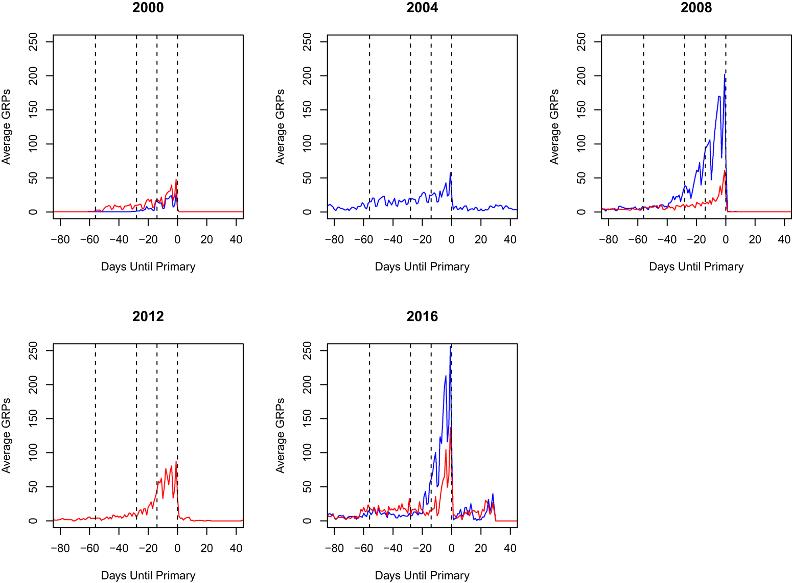
Figure 1. Temporal patterns of advertising—each line denotes the average number of GRPs across media markets, relative to the closest primary election in the media market. Blue lines denote the sum across all Democratic candidates and red lines denote the sum across all Republican candidates. The dotted vertical lines denote the primary election, 2 weeks before the primary election, 4 weeks before the primary election, and 8 weeks before the primary election.

In only one instance does the figure depart from these patterns. In 2016, we see a small temporary surge in the weeks following the primary election. The 2016 election campaign was particularly long, so though ads dropped off after the primary election was over, they picked up briefly in a number of swing states as candidates switched to general election campaigns. To deal with these limitations of the 2016 data, our tests only used observations before the primary election, so that our analysis could not be affected by early general election advertising, as was the case in 2016.¹¹

4.2. Favorability

In the first set of models, the dependent variable is favorability. We estimated the model using Ordinary Least Squares (OLS). We included a variable for whether the respondent and the candidate were of the same party, anticipating that respondents would rate their identified party’s candidates more favorably. We included respondent fixed effects to allow respondents to differ in how generously they graded the candidates. We included candidate fixed effects to allow the favorability of the candidates to vary with their characteristics (e.g. political experience), without needing to explicitly control for such characteristics.¹² Here (and throughout the paper), for the three ad variables, a 1-unit increase corresponds to a 1000 GRP increase in advertisements, which, in turn, corresponds to the entire population seeing an additional 10 ads.

We report results using three different windows for when an election is imminent—2 weeks, 4 weeks, and 8 weeks. The three windows are motivated by the results of Section 4.1—candidates appear to target the vast majority of their advertising to states that have an upcoming election. Advertising observed in a state that does not have an upcoming election is, therefore, very likely to be unpurposely targeted. Instead, such advertising is likely a by-product of residents of that state residing in a media market that overlapped a different state with an upcoming election.¹³

In the analysis, we used only respondents that were interviewed before the primary election in their state. The NAES only asked respondents their intended primary vote before the election while Gallup did continue to ask respondents to report their intended primary vote after the election. Our choice to omit respondents who were interviewed after their state’s primary stemmed from two concerns. First, the analysis of Section 4.1 suggests that some such respondents saw ads that were purposely targeted toward them due to early spending in the general election campaign (though even in this case, the ads were not purposely targeted in order to influence their primary votes). Second, the Gallup survey item was asked in such a way that respondents could have answered based on which candidate they had already voted for rather than which candidate they most preferred at the time they were interviewed. If a respondent reported who they voted for rather than who they preferred at the time of the interview, their responses could not be moved by advertisements aired after the primary.

The results are given in columns (1)–(3) of Table 2. We find that positive ads increase the favorability of the candidate running the ads. Negative ads similarly appear to increase the favorability of the candidate running the ad (though the effect is not statistically significant using the 8-week window) and negative ads appear to be more effective than positive ads.¹⁴ Being attacked does not appear to lower the favorability of the candidate running the ad.

Table 2. The effects of ads on favorability and candidate choice. Analyses include respondent and candidate fixed effects (columns 1–3) and candidate fixed effects (columns 4–6). Standard errors are in parentheses and are clustered by respondent in columns 1–3

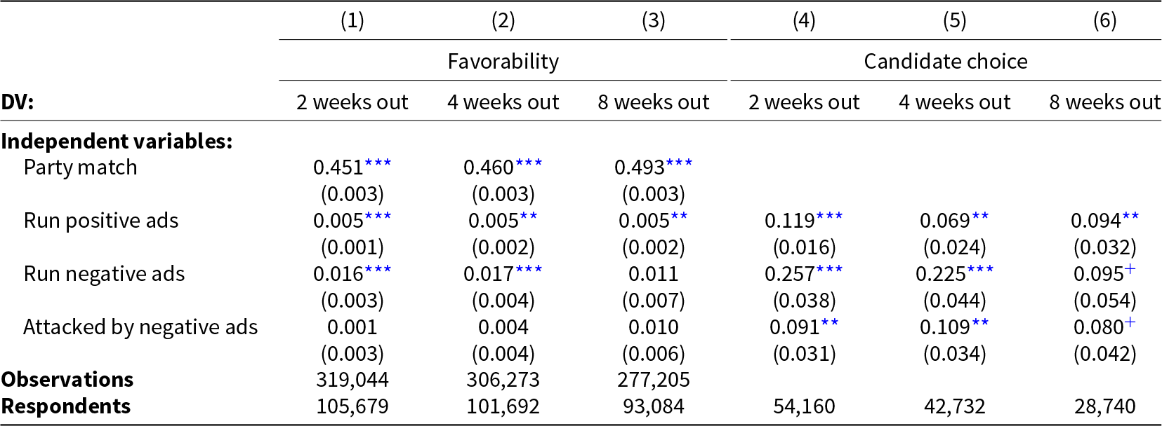
* indicates statistical significance at the 5% level. ** indicates statistical significance at the 1% level. *** indicates statistical significance at the 0.1% level. + indicates statistical significance at the 10% level.

To get a sense of the effect sizes, we considered the marginal effect of a change in advertising of 1000 GRPs. Based on the 4-week window, running 1000 GRPs of positive ads will increase the candidate’s favorability by 0.005 on the 0–1 scale. Running 1000 GRPs of negative ads will increase that candidate’s favorability by 0.017 on the 0–1 scale. In the time period we study, Obama purchased more GRPs than any other candidate—in the 2008 primary, he purchased 4816 GRPs in the average media market, compared to Hillary Clinton’s 3021 GRPs. Sanders, another high spending candidate, purchased 3779 GRPs in 2016. Romney purchased 1667 GRPs in 2008 and 2869 GRPs in 2012. In 2000, Bush was the highest spending candidate, purchasing 1377 GRPs. The vast majority of candidates (even relatively major ones) purchased less than 1000 GRPs. Given these numbers, for most candidates and most time periods, 1000 GRPs would entail a very substantial increase in their advertising. As such a campaign moves candidate favorability by between 0.005 and 0.017, we could conclude that in most cases, advertising has limited effects on favorability.

4.3. Candidate choice

We next analyzed the effect of advertising on candidate choice. In each case, the dependent variable was multinomial in nature, indicating the respondent’s preferred candidate in either the Democratic or Republican presidential primaries. Each model reported below is a conditional logit model. Each model also includes candidate-year fixed effects, to allow the vote share of candidates to vary with their characteristics (e.g. political experience), without needing to explicitly control for such characteristics. The results are given in columns (4)–(6) of Table 2. Running ads—both positive and negative—increase the latent utility of voting for a candidate. Being attacked also increases the latent utility of voting for a candidate. The raw coefficients are useful for determining whether there is statistical evidence of advertising effects, but neither the magnitude of the effects of positive and negative advertising, nor the effectiveness of positive relative to negative advertising, can be easily inferred from the coefficients, which we detail below.

Let u ₁ through u_J denote the utilities of candidates 1 through J. According to the conditional logit model, the vote share of candidate j is given by

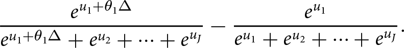
(1)\begin{equation} s_j = \frac{e^{u_j}}{e^{u_1} + e^{u_2} + \cdots + e^{u_J}}. \end{equation}

Let θ ₁ denote the effect of positive advertising, let θ ₂ denote the effect of negative advertising on the utility of the attacking candidate, and let θ ₃ denote the effect of negative advertising on the utility of the attacked candidate. Let Δ denote change in advertising above some baseline (e.g. 1000 GRPs). The change in the vote share of candidate 1 due to a change in positive advertising is given by

(2)\begin{equation} \frac{e^{u_1 + \theta_1 \Delta}}{e^{u_1 + \theta_1 \Delta} + e^{u_2} + \cdots + e^{u_J}} - \frac{e^{u_1}}{e^{u_1} + e^{u_2} + \cdots + e^{u_J}}. \end{equation}

The change in vote share of candidate 1 due to a change in the amount spent attacking candidate 2 is given by

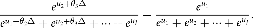
(3)\begin{equation} \frac{e^{u_1 + \theta_2 \Delta}}{e^{u_1 + \theta_2 \Delta} + e^{u_2 + \theta_3 \Delta} + \cdots + e^{u_J}} - \frac{e^{u_1}}{e^{u_1} + e^{u_2} + \cdots + e^{u_J}}. \end{equation}

The change in vote share of candidate 2 due to a change in the amount candidate 1 spends attacking candidate 2 is given by

(4)\begin{equation} \frac{e^{u_2 + \theta_3 \Delta}}{e^{u_1 + \theta_2 \Delta} + e^{u_2 + \theta_3 \Delta} + \cdots + e^{u_J}} - \frac{e^{u_1}}{e^{u_1} + e^{u_2} + \cdots + e^{u_J}}. \end{equation}

Each of these is a complicated function of the parameters $(\theta_1,\theta_2,\theta_3)$, the baseline utilities $(u_1, \ldots,u_J)$, and the size of the advertising change Δ. We deal with this complexity by calculating the effect of advertising in three ways. First, we consider the effect of a change in advertising in a close two-candidate race to provide a more direct comparison to advertising in presidential general elections. Second, we consider the effect of a change in advertising from a baseline matching the elections in our sample. Third, consider the effect of a small change in advertising, which exhibits less complexity.

As in Section 4.2, we consider the effect of a change in advertising of 1000 GRPs. We first report results for a hypothetical two candidate race where the candidates would be evenly matched if their adverting was balanced because this provides a more direct comparison to results reported in the literature for general elections. Increasing positive advertising by 1000 GRPs would lead to a candidate’s vote share increasing by between 1.7 and 3.0 percentage points (relying on a 2-week, 4-week, and 8-week windows). Increasing negative advertising by 1000 GRPs would lead to a candidate’s vote share increasing by between 0.4 and 4.1 percentage points. We can compare these results to those reported by Huber and Arceneaux (2007) and Gordon and Hartmann (2013) for Presidential elections. Huber and Arceneaux’s results imply that an increase of 1000 GRPs would lead to an increase of between 4.2% and 5.8% in a candidate’s vote share. Gordon and Hartmann’s results imply the same change would increase the candidate’s vote share by 1.5%. Our results are thus in between these two sets of results.

An important difference between Gordon and Hartmann (2013) and Huber and Arceneaux (2007) is the window of time over which they sum advertising. Gordon and Hartmann calculate the effect of advertisements run between between labor day and election day (a roughly 2-month period). Huber and Arceneaux calculate the effect of advertisements run between subsequent interviews (with a median of 28 days) in their panel analysis and within 4 weeks of the election in their cross-section analysis. If, as the literature has found (Gerber et al., 2011; Hill et al., 2013; Kalla and Broockman, 2022), advertising has a quickly decaying effect, we should expect to find smaller effects in Gordon and Hartmann than in Huber and Arceneaux if both designs are sound. Indeed, in their aggregate analysis, Huber and Arceneaux found that the effects we about 50% smaller when aggregating advertisements over a longer period of time. In light of this, our results are more directly comparable to Huber and Arceneaux, suggesting that (apart from differences due to the number of candidates and the baseline level of support we highlight below) advertising is somewhat less effective in primary elections.

We next report results that are calibrated to the elections in our sample. We started with a baseline of zero ad spending where the estimated candidate fixed effects allowed the baseline vote share to vary across candidates. For each candidate, we considered the effect of increasing the amount of positive advertising by 1000 GRPs, while holding everything else constant. For each candidate and each of their opponents, we considered the effect of increasing the amount of negative advertising directed at that opponent by 1000 GRPs. In each case, we report the change in vote share for the candidate running the ads. Full results are reported in Tables A.1 through A.6 in Online Appendix A.2.

Take the 2012 Republican primary. For every one of the candidates, running negative ads is more effective than running positive ads, regardless of which candidate is attacked by the negative ads. The largest effect comes from attacking low polling candidates, though the differences are typically small. Similar patterns hold for other years—negative advertising appears to be more effective than positive advertising, advertising is less effective for low polling candidates, and attack ads are more effective when they target low polling candidates.

To get a better understanding of the results in Tables A.1 through A.6, we consider the ratio of the effectiveness of positive to negative advertising by dividing equation (2) by equation (3), where to simplify, we let $C = e^{u_3} + \cdots + e^{u_J}$,

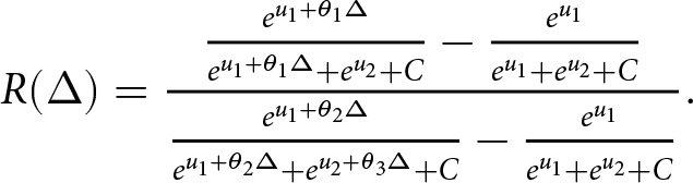(5)\begin{equation} R(\Delta) = \frac{\frac{e^{u_1 + \theta_1 \Delta}}{e^{u_1 + \theta_1 \Delta} + e^{u_2} + C} - \frac{e^{u_1}}{e^{u_1} + e^{u_2} + C}}{\frac{e^{u_1 + \theta_2 \Delta}}{e^{u_1 + \theta_2 \Delta} + e^{u_2 + \theta_3 \Delta} + C} - \frac{e^{u_1}}{e^{u_1} + e^{u_2} + C}}. \end{equation}

We approximate the effectiveness of positive relative to negative advertising by taking the limit of this expression as $\Delta \to 0$. This will provide a reasonable approximation for changes in advertising that do not have a very large effect on vote share. We obtain

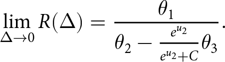(6)\begin{equation} \lim_{\Delta \to 0} R(\Delta) = \frac{ \theta_1}{\theta_2 - \tfrac{e^{u_2}}{e^{u_2} + C} \theta_3}. \end{equation}

Here, $\tfrac{e^{u_2}}{e^{u_2} + C}$ is the vote share of the attacked candidate, as a share of candidates 2 through J. Provided that $\theta_2 \gt \theta_3$ (which we indeed find in columns (4)–(6) of Table 2), the ratio will be positive. A ratio greater than 1 indicates that positive advertising is more effective and a ratio less than 1 indicates that negative advertising is more effective. The ratio will range from $\frac{\theta_1}{\theta_2 - \theta_3}$ (occurring when the attacked candidate has a much larger vote share than the other candidates) and $\frac{\theta_1}{\theta_2}$ (occurring when the attacked candidate has a negligible vote share).

We report results for three values of $\tfrac{e^{u_2}}{e^{u_2} + C}$ in Table 3. Using the 2-week and 4-week windows, we find that positive advertising is less effective than negative advertising. The ratio is statistically distinguishable from 1 when $\tfrac{e^{u_2}}{e^{u_2} + C}$ is equal to 0 or 0.5. Using the 8-week window, the ratio is very imprecisely estimated. The 8-week window eliminates much of the variation in advertising. Using this more restrictive window, we still find that advertising is effective, but we lose our ability to determine the relative effectiveness of positive and negative advertising.

Table 3. Relative effectiveness of positive advertising. Standard errors are in parentheses

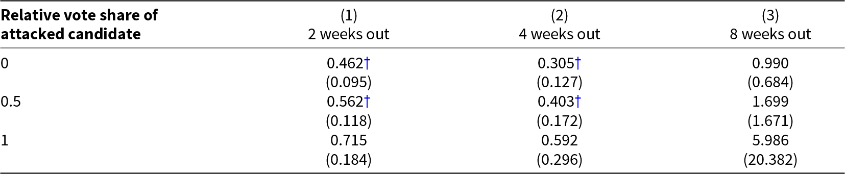
† indicates that the coefficient is statistically distinguishable from 1 at the 10% level.

We next move to examining the effect of negative advertising on the attacked candidate. In two candidate races, the effect on the attacked candidate is the negative of the effect on the attacking candidate. We thus omit the analysis of a hypothetical two candidate race since the results can be inferred directly from those already reported. In Tables A.7 through A.12 in Online Appendix A.1, we report the effect calibrated to elections in our sample. In the 2000 Democratic primary, Gore attacking Bradley costs Bradley 2.5 percentage points. This is equivalent to the gain to Gore (reported in Table A.1) due to the fact that the race involves two candidates. Considering instead the 2012 Republican primary, we find that all candidates gain when they are the subject of attack ads, with low polling candidates receiving the largest gains and high polling candidates receiving a negligible benefit from begin attacked. The results for other years indicate that high polling candidates are hurt when attacked by other high polling candidates, but otherwise candidates gain from being attacked.

To again get a better understanding of the results, we consider the marginal effect of a small change in negative advertising on the attacked candidate’s vote share. Taking the derivative of equation (4), we obtain

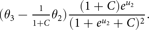(7)\begin{equation} (\theta_3 - \tfrac{1}{1+C} \theta_2) \frac{(1 + C) e^{u_2}}{(1 + e^{u_2} +C)^2}. \end{equation}

This represents the marginal effect of being attacked on the vote share of the attack candidate. The sign of the marginal effect will be the same as the sign of $(\theta_3 - \tfrac{1}{1+C} \theta_2)$. Here, $\tfrac{1}{1+C}$ is the vote share of the attacking candidate relative to candidates 3 through J. Suppose that $\theta_2 \gt 0$ and $\theta_3 \gt 0$, which is the case in all of our specifications. An attacked candidate will gain vote share if $\theta_3 \gt \tfrac{1}{1+C} \theta_2$ and will lose vote share if $\theta_3 \lt \tfrac{1}{1+C} \theta_2$. If $\theta_3 \ge \theta_2$, the attacked candidate will always gain vote share, but we don’t find this in any of our specifications. If $\theta_3 \lt \theta_2$, there is a crossover point where low polling candidates gain by being attacked and high polling candidate are hurt when attacked. This is indeed consistent with patterns in Tables A.7 through A.12. From the specifications in columns (4) through (6) of Table 2, we find crossover points of 0.353, 0.483, and 0.854, respectively. In Table A.8, for example, the attacked candidate looses vote share precisely when $\tfrac{1}{1+C} \lt \frac{\theta_3}{\theta_2} = 0.483$. The results for the 2-week and 4-week windows are statistical distinguishable from both 0 and 1, while the result for the 8-week window is not statistical distinguishable from either 0 or 1. The approximation based on small changes in advertising thus implies that high polling candidates are hurt when attacked and low polling candidates are helped when attacked.¹⁵

Summarizing our findings for the relative effectiveness of negative advertising, we find that positive advertising is less effective than attacking a low polling candidate, and we can reject the null hypothesis that positive and negative advertising are equally effective in this case. We find that positive advertising is somewhat less effective than attacking a high polling candidate. The point estimates indicate that positive advertising is 72% as effective (using a 2-week window) and 59% as effective (using a 4-week window), with the estimate based on an 8-week window very imprecisely estimated. The results for attacking a high polling candidate are most comparable to the results for general elections.¹⁶ The closest result in the literature is reported in Gordon et al. (2023), who study advertising by the presidential candidates in the 2000 and 2004 elections. They find that positive advertising is about 80% as effective as negative adverting, but the relative effectiveness of positive advertising is not statistically distinguishable from 1. These results are quite similar to what we find for primary elections. In their meta analysis, Lau et al. (2007) report that there is a great deal of variability in the effects of negative advertising on vote choice. Most of the studies they report are survey experiments. The three studies that use similar advertising data report varying results.¹⁷

4.4. Perceived viability

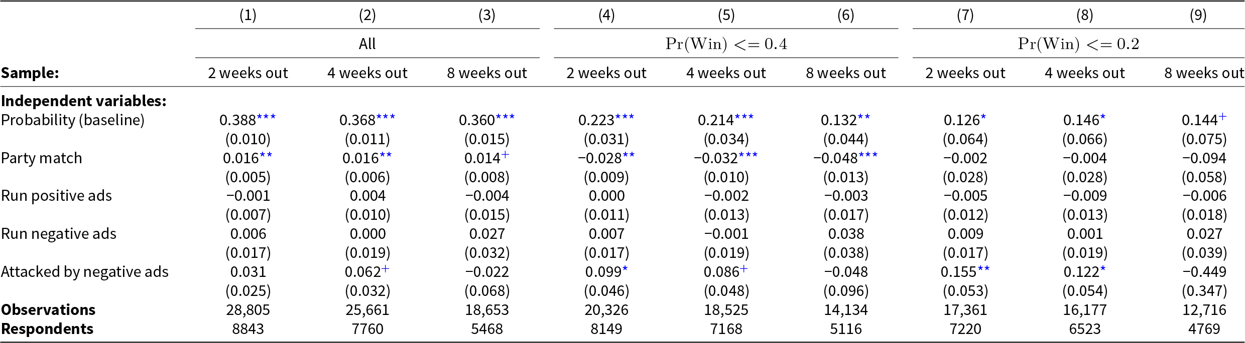
To directly test whether being attacked increases a candidate’s perceived viability, we rely on variables available in the 2000 and 2004 NAES. We estimated the model using OLS and we included as control variables a benchmark for the probability that the candidate would win the primary based on prediction markets, as well as whether the respondent and the candidate were of the same party. As before, we included respondent fixed effects and candidate fixed effects. We report results using three different windows for when an election is imminent—2 weeks, 4 weeks, and 8 weeks. We report results for the full sample, for candidates whose objective probability of winning the primary was less than 0.4, and for candidates whose objective probability of winning the primary was less than 0.2. The later two sub-samples are motivated by the fact that candidates that are frontrunners are likely to be nearly universally perceived as likely to win the primary. Instead, it is in determining who is a plausible challenger to a frontrunner where negative advertising has room to have an effect. They are also motivated by the estimates in Section 4.3, which suggest that only low polling candidates benefited from being attacked.

The results are given in Table 4. In the full sample, there is weak evidence that being attacked increases a candidate’s perceived viability—only in the 4-week window is the effect positive and statistically significant, and in that case, the effect is only statistically significant at the 10% level. When we move to the sample of candidates whose objective probability is less than 0.4, we find an effect that is positive and statistically significant in the 2-week and 4-week windows. In the sample where the objective probability is less than 0.2, we find stronger evidence that being attacked increases a candidates perceived viability—the effect is positive and statistically significant with the 2-week window (at the 1% level) and the 4-week window (at the 5% level). The results for the 8-week window continue to be ambiguous, with a statistically insignificant effect and a large standard error.

Table 4. The effects of ads on perceived probability of winning the primary. Analyses include respondent and candidate fixed effects. Standard errors clustered by respondent are in parentheses

* indicates statistical significance at the 5% level.

** indicates statistical significance at the 1% level.

*** indicates statistical significance at the 0.1% level.

+ indicates statistical significance at the 10% level.

Summarizing our findings, we have evidence that in terms of vote share, ads are effective, negative ads are relatively more effective, and low polling candidates often benefit when they are attacked. Looking at favorability, positive ads and negative ads both are both effective for the candidate running the ads, with negative ads being more effective. Attacked candidates are neither helped nor hurt. This can be understood in the following way. The measure of favorability arguably is insulated from concerns of perceived viability while vote intent arguably incorporates these concerns. Finding that low polling candidates increase their vote share when attacked is thus suggestive that being attacked increases the low polling candidates’ perceived viability. We indeed find that being attacked increases a candidate’s perceived viability, with the evidence being strongest in the sample of candidates who are unlikely to win the primary.

4.5. Robustness

In the Online Appendix, we report a number of robustness checks on the main results. In Online Appendix A.3, we report results where we construct the independent variables based on ad counts rather than GRPs. We report results with candidate-month fixed effects instead of candidate fixed effects. We consider a log specification for advertising to allow for diminishing returns to advertising. We consider results that don’t rely on respondents residing in states with early contests. We consider independent variables that allow advertising to have an effect over a 2-week or 8-week period (instead of the baseline of 4 weeks). Finally, we consider a binary measure of favorability as the dependent variable. Our substantive conclusions are robust to these alternative modeling choices. In Online Appendix A.4, we allow primarily negative ads and contrast ads to have different effects on favorability and vote intent. We don’t find much evidence that primarily negative ads and contrast ads are differentially effective.

5. Conclusion

In this article, we sought to answer four questions. Is television advertising effective in presidential primary elections? How does the effectiveness of television advertising in primary elections compare to its effectiveness in general elections? Are positive and negative advertising differentially effective in primary elections? What are the mechanisms behind the effectiveness of advertising in presidential primary elections?

We found clear evidence that television advertising is effective. Advertising increases the favorability of candidates and increases the likelihood that respondents intend to vote for those candidates. Moreover, the effects appear to be of the same order of magnitude as other scholars have found for general elections, though the effects sizes are somewhat smaller than what the study with the most similar methodology found (Huber and Arceneaux, 2007). Primaries, however, feature far more variation in the strength of candidates than general elections—since 2000, presidential elections have been fairly close among the two major parties. Advertising appears to be more effective for high polling candidates than for low polling candidates.

Negative advertising appears to be more effective in increasing a candidate’s favorability and in increasing the likelihood that respondents intend to vote for that candidate. Moreover, while high polling candidates are hurt by attack ads, low polling candidates are helped. This last result speaks directly to the mechanisms underlying the effectiveness of advertising—being attacked appears to increase the perceived viability of low polling candidates. Evidence for this mechanism come from two different sources. Indirect evidence comes from the robust finding that low polling candidates increase their vote share when attacked, which in our theoretical framework can only be explained by increased perceived viability. Direct evidence comes from the 2000 and 2004 NAES where we found that for non-frontrunner candidates, being attacked increased survey respondents’ estimates of the likelihood that the candidate would win the primary.