Research on natural hedge strategy of insurance companies based on combination “Variance” effect

Abstract

Longevity risk significantly impacts the reserve adequacy ratio of annuity issuers, thereby reducing product profitability. Effectively managing this risk has thus become a priority for insurance companies. A natural hedging strategy, which involves balancing longevity risk through an optimised portfolio of life insurance and annuity products, offers a promising solution and has attracted considerable academic attention in recent years. In this study, we construct a realistic portfolio scenario comprising annuities and life insurance policies across various ages and genders. By applying Cholesky decomposition, we transform the portfolio into an uncorrelated linear model. Our objective function minimises the variance in portfolio value changes, allowing us to explore the impact of mortality on longevity risk mitigation through natural hedging. Using actuarial mathematics and the Bayesian MCMC algorithm, we analyse the factors influencing the hedging effectiveness of a portfolio with minimised variance. Empirical findings indicate that the optimal life-to-annuity ratio is influenced by multiple factors, including gender, age, projection period, and forecast horizon. Based on these findings, we recommend that insurance companies adjust their business structures and actively pursue product innovation to enhance longevity risk management.

1. Introduction

With economic development and social progress, China has seen significant improvements in medical and health conditions, as well as in living standards, leading to a continuous increase in life expectancy. According to the latest data from the National Bureau of Statistics, China’s average life expectancy reached 77.93 years in 2020, with men averaging 75.37 years and women 80.88 years. “Longevity” has thus become a defining characteristic of China’s population. Longevity risk arises when future life expectancy surpasses current expectations, affecting the financial planning of individuals and corporations alike. For life insurance companies, longevity risk influences annuity reserves, thereby reducing the profitability of annuity products. This risk is long-term, systematic, and accumulative, and it cannot be mitigated by traditional risk management methods. Consequently, managing longevity risk effectively remains a primary focus for insurance companies. One promising approach is the natural hedging strategy, which has also gained considerable attention in academic circles in recent years. This strategy leverages the inverse relationship between losses and gains associated with mortality changes in life insurance and annuity products. Not only does natural hedging help life insurance companies reduce risk management costs, it also demonstrates strong practical feasibility, making it an ideal method for managing longevity risk.

The theoretical foundation of natural hedging can be traced back to Marceau and Gailardetz (1999), where the authors measured the longevity risk of life insurance contracts, annuity contracts, and their combinations under conditions of stochastic interest and mortality rates. Later, research by Milevsky and Promislow (2001) further validated the opposing impacts of longevity risk on the life insurance and annuity businesses, respectively. However, the portfolio characteristics identified in these studies were not immediately applied to longevity risk management within life insurance companies. It was only with the work of Cox and Lin (2007) that a formal proposal emerged to adjust the structural balance of life insurance and annuity portfolios to mitigate the longevity risk embedded in such portfolios. Subsequently, Plat (2011) introduced the duration-convexity matching theory, addressing limitations in existing methodologies. Plat derived formulae for calculating the duration and convexity of effective mortality rates, providing a method to efficiently determine the optimal balance of a simulated portfolio of annuities and life insurance policies.

With a growing understanding of longevity risk and the advancement of quantitative management tools, recent years have seen an increase in scholarly exploration of natural hedging strategies from diverse perspectives. Internationally, Tsai et al. (2010) employed the “conditional value at risk minimization (CVaRM)” approach alongside the Cairns-Blake-Dowd (CBD) mortality model to propose a longevity risk hedging strategy. Wang et al. (2010) introduced an immune model using stochastic dynamic mortality to calculate the optimal portfolio ratio of life insurance and annuity products for hedging against longevity risk. Using empirical mortality data, Wang et al. (2013) provided a practical natural hedging model for insurers, with the advantage of addressing the impact of mispricing on longevity risk. In China, Huang and Wang (2011) applied the value at risk (VaR) method and the Age-Period-Cohort model to design a natural hedging strategy for managing longevity risk in China, further analysing the effects of interest rates, underwriting age, payment methods, and other factors on the optimal product mix. Jin (2013) explored a natural hedging strategy using the Lee-Carter model and the CVaR method, incorporating a stochastic interest rate. Through empirical calculations, Jin found that random interest rates influence whether insurers can fully hedge longevity risk. Wei and Song (2014) utilised the CBD model to simulate population mortality rates and applied the generalised method of moments (GMM) to estimate the interest rate model, comparing the effectiveness of natural hedging under fixed and random interest rates. Their results indicate that strategies designed under fixed interest rates may face hedging insufficiencies under stochastic interest rate conditions. Zeng et al. (2015) linked a demand model, which determines the actual sales mix of products, with a natural hedging model that optimises the mix by modelling. They analysed the price adjustment effect, providing optimal pricing strategies for life insurance and annuity products and examining the impact of interest rates, underwriting age, gender, and other factors on natural hedging strategies.

Additionally, several scholars have investigated the effectiveness of natural hedges in managing longevity risk. For example, Gatzert and Wesker (2012) evaluated the effectiveness of natural hedges by considering the correlation among systematic risk, unsystematic risk, basis risk, and adverse selection. Li and Haberman (2015) assessed the effectiveness of natural hedges between annuity and life insurance products using the Poisson Lee model, the Poisson common factor model, the product ratio model, and historical simulation. Luciano et al. (2017) examined the natural hedging effects across both single and multiple generations facing longevity and interest rate risks by analysing mortality variations across different years, finding that intergenerational hedging through annuity and life insurance products is effective for longevity risk management. In Chinese research, Duan and Jie (2017) studied the impact of longevity risk on reserve valuation for life insurance and annuity products, based on adjustments to the empirical life tables used in China’s life insurance industry. Hu (2019) proposed an age-based hedging strategy that explores the effectiveness of natural hedging on annuity products, applying mortality immunisation theory and the duration rule. Duan (2019) used hedge elasticity to quantify the hedging effect across different product portfolios by constructing a mortality model and analysed the long-term impact of interest rate changes on hedging effectiveness.

In summary, the literature on longevity risk hedging, both domestically and internationally, offers a wealth of insights and methodologies worthy of reference. However, natural hedging research still faces several challenges. First, the availability of mortality rate data in China is limited, with shorter time spans that do not meet the requirements of time series models, preventing the direct application of the Lee-Carter model, which requires extensive historical data. Second, existing research often focuses either on the optimal hedging ratio for single-life annuities (e.g., Huang & Wang, 2011; Wei & Song, 2014; Li & Haberman, 2015) or neglects the risk correlations among multiple products in diversified portfolios (e.g., Jin, 2013; Duan, 2019). This oversight fails to capture the gender- and age-specific risk correlations in products, which may differ significantly from the actual multi-product portfolios held by insurance companies, thus limiting the practical applicability of the findings.

To address these issues, this study introduces improvements in several areas. First, regarding product mix, we investigate the covariance relationships among male and female annuities and life insurance products. By applying Cholesky decomposition, we transform the Brownian motion associated with each product’s value into four independent linear combinations, facilitating a more realistic simulation of the effects of mortality-related changes on insurance portfolios. Based on this approach, we measure the impact of mortality and interest rates on the portfolio using the variance in portfolio value changes and identify the optimal annuity and life insurance mix to minimise this variance and hedge against longevity risk. Second, in terms of mortality simulation, this study employs the Bayesian MCMC method as a unified framework and uses WinBUGS (Scollnik, 2001) to estimate and forecast mortality parameters, calculate mortality duration and convexity, and determine the optimal product portfolio allocation. By generating extensive convergent sample data, this approach mitigates the limitations of historical data, enhances mortality forecasting accuracy, and enables more precise longevity risk measurement.

We will first present our modelling approach in Section 2. Section 2 details the mathematical models and their underlying assumptions, with particular emphasis on how variance effect measures are utilised to optimise the composition of insurance portfolios. Section 3 focuses on the forecasting methodology, describing the parameter estimation process and explaining how Bayesian MCMC methods are employed for mortality parameter estimation and projection. These projections are then used to determine optimal portfolio allocations. In Section 4, we report our empirical findings, investigating the effectiveness of combining life insurance and annuities as a hedging strategy across different genders and age groups. Special attention is given to the variations in the proportions of male and female life insurance portfolios with respect to age, as well as the impact of forecast horizons on the optimal hedging shares of life insurance and annuities. Finally, Section 5, we summarise the key findings of our study, discuss their theoretical contributions and practical implications, and propose potential directions for future research.

2. Modelling

The Lee-Carter model, proposed by Lee and Carter (1992), is the most commonly used mortality model in academic research. Known for its ease of implementation and low prediction error, the Lee–Carter model is widely applied in mortality trend fitting and forecasting. This study employs the classic Lee–Carter model to predict mortality rates, assuming that the natural logarithm of the central mortality rate at integer age x and calendar year t satisfies:

(1) $$ \mathit{ln}({m}_{x,t})={\alpha }_{x}+{\beta }_{x}{k}_{t}$$

In this context, $ {\alpha }_{x}$ represents the age-specific mortality factor at age x, $ {\beta }_{x}$ denotes the improvement factor for age-specific mortality, and $ {k}_{t}$ is the mortality rate index that changes over time, measuring the rate of mortality improvement. To ensure the identifiability of Equation (1), parameters $ {\beta }_{x}$ and $ {k}_{t}$ must satisfy the following constraints:

$$\mathop \sum \limits_{x}{\beta }_{x}=1\ {\rm and}\ \mathop \sum \limits_{t}{k}_{t}=0$$

In the Lee–Carter model, the time-effect index $ {k}_{t}$ can be estimated using an ARIMA (0,1,0) process, as follows:

(2) $$ {k}_{t}-{k}_{t-1}={u}_{k}+{e}_{t}$$

where $ {e}_{t} \! \sim \! N(0,{\sigma }_{k}^{2})$ . The Lee–Carter model is fitted using the Singular Value Decomposition (SVD) method proposed by Lee and Carter (1992).

We assume that the insurance company’s portfolio includes annuities and life insurance policies for policyholders of various ages and genders. Specifically, at time 0, a set of annuities and life insurance policies is issued to individuals of different ages, denoted by x, where ω represents the maximum age among all policyholders at that time. The primary factor influencing the total portfolio value is mortality. Therefore, the total value of the life insurance company’s portfolio can be expressed as:

(3)

$V\left( {m_x^{Ai}\left( t \right)} \right)$ and $V\left( {m_x^{Li}\left( t \right)} \right)$ represent the value of annuity and life insurance policies respectively, while $N_x^{Ai}$ and $N_x^{Li}$ represent the number of annuity and life insurance policies issued by life insurance companies respectively, where i = 1 and 2 represent male and female policies respectively.

According to documents such as Biffis et al. (2010) and Wang et al. (2013), the continuous time form of the ARIMA (0,1,0) process of the time effect index $ {k}_{t}\rm{}$ can be expressed as:

(4) $$ d{k}_{t}={u}_{k}dt+{\sigma }_{k}d{Z}_{k}\left(t\right)$$

Assuming that $ \left({Z}_{r}\right(t){)}_{t=0}^{T}$ is a standard Brownian motion, the logarithmic central mortality rate at integer age x in calendar year t can be expressed as:

(5) $$ \eqalign{d\,\mathit{ln}({m}_{y,t})& =\mathit{ln}({m}_{y,t+dt})-\mathit{ln}({m}_{y,t})={\beta }_{y}({k}_{t+dt}-{\! k}_{t}) \cr & ={\beta }_{y}d{k}_{t}={\beta }_{y}({u}_{k}dt+{\sigma }_{k}d{Z}_{k}(t\left)\right)}$$

Simultaneously, based on Ito’s lemma, the dynamic logarithm of the mortality rate can be transformed into a dynamic mortality rate, as shown below:

(6) $$d\left( {{m_{y,t}}} \right) = d\left( {{e^{ln({m_{y,t}})}}} \right) = {m_{y,t}}d\left( {ln\,{m_{y,t}}} \right) + {1 \over 2}{m_{y,t}}d{(ln\,{m_{y,t}})^2}= {m_{y,t}}({\beta _y}{u_k}dt + {\beta _y}{\sigma _k}d{Z_k}(t)) + {1 \over 2}{m_{y,t}}\left( {\beta _y^2\sigma _k^2dt} \right)= ({m_{y,t}}{\beta _y}{u_k} + {1 \over 2}{m_{y,t}}\beta _y^2\sigma _k^2)dt + ({m_{y,t}}{\beta _y}{\sigma _k})d{Z_k}(t)$$

If y=x + t, Equation (6) can be written as:

(7) $$d\left( {{m_{x,t}}} \right) = ({m_{x,t}}{\beta _{x + t}}{u_k} + {1 \over 2}{m_{x,t}}\beta _{x + t}^2\sigma _k^2)dt + ({m_{x,t}}{\beta _{x + t}}{\sigma _k})d{Z_k}(t)$$

In order to capture the covariance structure of mortality rates for annuities and life insurance products, we assume that the death risk factors $ {Z}_{k}^{A,2}$ , $ {Z}_{k}^{A,1}$ , $ {Z}_{k}^{L,2}$ and $ {Z}_{k}^{L,1}$ for annuities and life insurance policies are standard Brownian motion that satisfies the following relationship, where ρ is the correlation between them:

$$\left[ {\matrix{ {Z_k^{A,2}\left( t \right)} \cr {Z_k^{A,1}\left( t \right)} \cr {Z_k^{L,2}\left( t \right)} \cr {Z_k^{L,1}\left( t \right)} \cr } } \right]\sim{N_4}\left( {\left[ {\matrix{ 0 \cr 0 \cr 0 \cr 0 \cr } } \right]\left[ {\matrix{ 1 & {{\rho _{12}}} & {{\rho _{13}}} & {{\rho _{14}}} \cr {{\rho _{12}}} & 1 & {{\rho _{23}}} & {{\rho _{24}}} \cr {{\rho _{13}}} & {{\rho _{23}}} & 1 & {{\rho _{34}}} \cr {{\rho _{14}}} & {{\rho _{24}}} & {{\rho _{34}}} & 1 \cr } } \right]t} \right)$$

$ {N}_{4}(a,b)$ represents a four-dimensional multivariate normal distribution with a mean vector a and a covariance matrix b. Then, according to the Cholesky decomposition, i.e. the decomposition of a symmetric positive definite matrix into the product of a lower triangular matrix and its transposition, the relevant Brownian motion $ {Z}_{k}^{A,2}$ , $ {Z}_{k}^{A,1}$ , $ {Z}_{k}^{L,2}$ and $ {Z}_{k}^{L,1}$ can be decomposed into four independent linear combinations of Brownian motion $ {Z}_{k1}$ , $ {Z}_{k2}$ , $ {Z}_{k3\rm{}}$ and $ {Z}_{k4}$ .

$$\left[ {\matrix{ {dZ_k^{A,2}\left( t \right)} \cr {dZ_k^{A,1}\left( t \right)} \cr {dZ_k^{L,2}\left( t \right)} \cr {dZ_k^{L,1}\left( t \right)} \cr } } \right] = \left[ {\matrix{ 1 & 0 & 0 & 0 \cr {{a_{21}}} & {{a_{22}}} & 0 & 0 \cr {{a_{31}}} & {{a_{32}}} & {{a_{33}}} & 0 \cr {{a_{41}}} & {{a_{42}}} & {{a_{43}}} & {{a_{44}}} \cr } } \right]\left[ {\matrix{ {d{Z_{k1}}\left( t \right)} \cr {d{Z_{k2}}\left( t \right)} \cr {d{Z_{k3}}\left( t \right)} \cr {d{Z_{k4}}\left( t \right)} \cr } } \right]$$

The specific calculation is:

$${a_{jj}} = {\left( {{\rho _{jj}} - \sum\limits_{k = 1}^{j - 1} {a_{jk}^2} } \right)^{{1 \over 2}}}$$

$${\,\,\,a_{ij}} = {{{\rho _{ij}} - \sum\nolimits_{k = 1}^{j = 1} {{a_{jk}}{a_{ik}}} } \over {{a_{jj}}}}$$

To examine the impact of changes in the total insurance portfolio value relative to the mortality rate, we apply Ito’s lemma again, incorporating the previously derived Cholesky decomposition coefficient. The resulting formula is:

(8) $$dV\left( t \right) = {\mathop\sum \limits_{s = L,A}}\;{\mathop\sum \limits _{g = {\rm{1}},{\rm{2}}}}\mathop\sum \limits_{x = i}^\omega N_x^{s,g}{{\partial V_x^{s,g}} \over {\partial m_x^{s,g}}}dm_x^{s,g}\left( t \right) + {\mathop\sum \limits _{s = L,A}}\;{\mathop\sum \limits _{g = {\rm{1}},{\rm{2}}}}\mathop\sum \limits _{x = i}^\omega {1 \over 2}N_x^{s,g}{{{\partial ^2}V_x^{s,g}} \over {\partial m{{_x^{s,g}}^2}}}{(dm_x^{s,g}(t))^2}={Q}_{0t}dt+ \mathop\sum \limits _{i=1}^{4}{Q}_{it}d{Z}_{ki}\left(t\right)$$

Among them:

(9) $${Q_{0t}} = {\mathop\sum \limits_{s = L,A}}\;{\mathop\sum \limits _{g = {\rm{1}},{\rm{2}}}}\mathop\sum \limits _{x = i}^\omega N_x^{s,g}{{\partial V_x^{s,g}} \over {\partial m_x^{s,g}}}\left( {m_x^{s,g}\left( t \right)\beta _{x + t}^{s,g}u_k^{s,g} + {1 \over 2}m_x^{s,g}\left( t \right)\beta {{_{x + t}^{{s,g}^2}}}\sigma {{_k^{{s,g}^2}}}} \right) + {1 \over 2}N_x^{s,g}{{{\partial ^2}V_x^{s,g}} \over {\partial m{{_x^{{s,g}^2}}}}} \times {\left(m_x^{s,g}\left( t \right)\beta _{x + t}^{s,g}\sigma _k^{s,g}\right)^2}$$

Further, let

$$\sum\limits_{x \in \varpi } {{{\partial V_x^{A,2}} \over {\partial m_x^{A,2}}}} m_x^{A,2}(t)\beta _{x + t}^{A,2}\sigma _k^{A,2} = {\phi _{A,2}}\mathop \sum \limits_{x \in \varpi } {{\partial V_x^{A,1}} \over {\partial m_x^{A,1}}}m_x^{A,1}\left( t \right)\beta _{x + t}^{A,1}\sigma _k^{A,1} = {\varphi _{A,1}}$$

$$\sum\limits_{x \in \varpi } {{{\partial V_x^{L,2}} \over {\partial m_x^{L,2}}}} m_x^{L,2}(t)\beta _{x + t}^{L,2}\sigma _k^{L,2} = {\phi _{L,2}}\mathop \sum \limits_{x \in \varpi } {{\partial V_x^{L,1}} \over {\partial m_x^{L,1}}}m_x^{L,1}\left( t \right)\beta _{x + t}^{L,1}\sigma _k^{L,1} = {\varphi _{L,1}}$$

Where the parameters $ {\varphi }_{s , g}$ (s=A, L, g = 1,2) are defined herein as the combined duration of the force of mortality, from which:

$$ {Q}_{1t}={N}_{x}^{A,2}{*}{\varphi }_{A,2}+{a}_{21}{*}{N}_{x}^{A,1}{*}{\varphi }_{A,1}+{a}_{31}{*}{N}_{x}^{L,2}{*}{\varphi }_{L,2}+{a}_{41}{*}{N}_{x}^{L,1}{*}{\varphi }_{L,1}$$

$$ \!\!\!\!\!\!\!\!\!\!\!\!\!\!\!\!\!\!\!\!\!\!\!\!\!\!\!\!\!\!\!{Q}_{2t}={a}_{22}{*}{N}_{x}^{A,1}{*}{\varphi }_{A,1}+{a}_{32}{*}{N}_{x}^{L,2}{*}{\varphi }_{L,2}+{a}_{42}{*}{N}_{x}^{L,1}{*}{\varphi }_{L,1}$$

$$ \!\!\!\!\!\!\!\!\!\!\!\!\!\!\!\!\!\!\!\!\!\!\!\!\!\!\!\!\!\!\!\!\!\!\!\!\!\!\!\!\!\!\!\!\!\!\!\!\!\!\!\!\!\!\!\!\!\!\!\!\!\!\!\!\!\!\!\!\!\!\!\!\!{Q}_{3t}={a}_{33}{*}{N}_{x}^{L,2}{*}{\varphi }_{L,2}+{a}_{43}{*}{N}_{x}^{L,1}{*}{\varphi }_{L,1}$$

To estimate the first and second derivatives of mortality, we can apply the concepts of duration and convexity. According to actuarial theory, the pricing formula for a standard life annuity policy is given as:

(10) $${\ddot a_{x:\bar n|}} = \mathop \sum \limits_{k = 0}^{n - 1} {}_k^{}{p_x} \times {e^{ - \delta k}} = \mathop \sum \limits_{k = 0}^{n - 1} {e^{ - \mathop \int \nolimits_0^k {\mu _x}\left( t \right)dt}} \times {e^{ - \delta k}}$$

Where ${\ddot a_{x:\bar n|}}$ represents the annuity factor for an insured person aged x who receives payments at the beginning of each period for n years, which is represented as $ {m}_{x}\left(t\right)$ in this paper, denotes the mortality rate of a person aged x at time t. $ {{}_{t}p}_{x}$ represents the probability that a person aged x will survive to age x + t, given by the formula: . However, since $ {{}_{t}p}_{x}$ and $ {\int }_{0}^{k}{\mu }_{x}\left(t\right)dt$ do not share a common factor in the formula, this paper refers to the method in the actuarial literature by Tsai and Lin (2013) and Lin and Tsai (2014). It assumes that the mortality rate $ {\mu }_{x}\left(t\right)$ undergoes a constant adjustment, represented as $ {{m}_{x}}^{\bullet }\left(t\right)={m}_{x}\left(t\right)+\lambda $ , so that $ {{}_{k}p}_{x}$ becomes:

(11) $$ {{{}_{k}p}_{x}}^{\bullet}={e}^{-{\int }_{0}^{k}\left[{\mu }_{x}\left(t\right)+\lambda \right]dt}={{}_{k}p}_{x}\times f\left(k,\lambda \right)$$

In this context, f(k, $ \lambda $ ) is called the adjustment function, which can be expanded in a Taylor series as: $f(k,\lambda ) = {e^{ - \lambda k}} = 1 - k\lambda + {k^2}{{{\lambda ^2}} \over 2} + \cdots + o\left( {{\lambda ^2}} \right)$ ; determined by the constant adjustment $ \lambda $ of the annuity for the survival of an individual aged x with duration k and mortality rate $ {\mu }_{x}\left(t\right)$ . Setting:

$$d\left( k \right) = - {{\partial f(k,\lambda )} \over {\partial \lambda }}{\big|_{\lambda = 0}} = k$$

The mortality duration of an annuity policy can be expressed as:

$$D\left[ {{{\ddot a}_{x:\bar n|}}({\mu _x})} \right] = \mathop \sum_{k = 0}^{n - 1} \,d\left( k \right) \times {}_k^{}{p_x} \times {e^{ - \delta k}}$$

Here, the concepts of mortality duration and convexity are used, analogous to dollar duration. These metrics represent the sensitivity of insurance product prices (such as life insurance and annuities) to changes in mortality. Based on the definitions of duration and actuarial mathematics:

(12) $$D\left( {A_{x:\bar n|}^1} \right) = - \left[ {d \times D\left( {{{\ddot a}_{x:\bar n|}}} \right) + D\left( {{}_n^{}{E_x}} \right)} \right]$$

where $ {{}_{n}E}_{x}={v}^{n}\times {{}_{n}p}_{x}$ , indicating that the duration of a life insurance policy is inversely related to that of an annuity. Therefore, we derive:

$${{\partial V_x^A} \over {\partial m_x^A}} = D\left[ {{{\ddot a}_{x:\bar n|}}({m_x})} \right],\,\,{{\partial V_x^L} \over {\partial m_x^L}} = D\left( {A_{x:\bar n|}^1} \right)$$

Thus, we can obtain the first- and second-order derivatives of the mortality rate using the results from duration analysis.

Based on the theoretical derivations above, we can determine the variance of the total value change in the insurance portfolio of the life insurance company. That is, the objective function f is expressed as:

(13) $$ f\left({N}_{x}^{s,g}\right)=Var\left(dV\right(t\left)\right)= \mathop \sum \limits_{j=1}^{4}({Q}_{jt}{)}^{2}, \,\, s=A,L,g=\rm{1,2},x\le \omega $$

In this paper, the objective function is defined as the variance effect of longevity risk. We identify the main components of this variance effect based on the effective duration of annuities and life insurance products, as well as the Cholesky decomposition coefficient. A minimum value of this objective function indicates that the insurance portfolio is minimally affected by changes in mortality, implying a lower impact of longevity risk. This effect is clearly a variable influenced by the parameters of the Lee–Carter model; specifically, a value derived from the first and second derivatives of the mortality rates for annuity and life insurance policies. Insurance companies aim to minimise the variance of portfolio value fluctuations due to mortality changes by optimally selecting the number of annuities and life insurance policies and employing natural hedging mechanisms to mitigate longevity risk.

3. Mortality Projections

3.1. Introduction of Forecast Methods

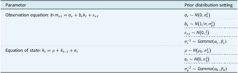
Given the limited availability of mortality statistics in China and limitations in the traditional parameter estimation methods of the Lee–Carter model, this paper employs the classic Lee–Carter model with Bayesian parameter estimation via the Markov Chain Monte Carlo (MCMC) method. The core idea of this approach is to construct a stationary Markov chain and sample from it. Once the sampling converges, statistical inference can be conducted based on the numerical characteristics of the parameters observed in these samples. Additionally, WinBUGS software is used to support the application of the Bayesian MCMC method. The Bayesian approach remains grounded in the original Lee–Carter model while re-estimating its parameters. The original model is expressed as:

(14) $$ \mathit{ln}\, {m}_{x,t}={\alpha }_{x}+{\beta }_{x}{k}_{t}+{\varepsilon }_{x,t}$$

The parameters retain the same definitions as in Equation (1). The state equation for simultaneous simulation is:

(15) $$ {k}_{t}=u+{k}_{t-1}+{e}_{t}$$

Here, u is the drift term, and e_t is the random error term. The Table 1 shows the prior distributions of some parameters related to the observation process:

Table 1. Prior distributions on parameters in the Bayesian model

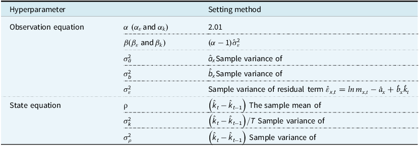
$ {\sigma }_{a}^{2}$ and $ {\sigma }_{b}^{2}$ are the variance of a priori distribution respectively, na being the number of age groups. For the parameters in the above prior distribution, i.e. the super parameter settings are shown in the Table 2.

Table 2. Hyperparameter settings for the Bayesian model

3.2. Results of Parameter Estimation

This paper selects the national historical data of male and female mortality rates for a total of 25 years from 1995 to 2019. The selected data are from the China Demographic Yearbook. In order to maintain consistency, we take 90+ years as the upper limit of age, and aggregate the statistical tables of data of 100 years old and above in some years, and classify them into the category of 90+ years old.

Firstly, we ran an MCMC simulation in WinBUGS to generate 11,000 posterior samples for each parameter. The first 1,000 samples were discarded as burn-in, and the remaining 10,000 samples were used to compute the parameter estimates. 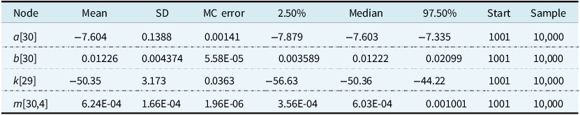In the process of single simulation sampling, we obtained a total of 2,115 estimation values of testing parameters through software, which are $ {a}_{x}$ (91), $ {b}_{x}$ (91), $ {k}_{x}$  (45), $ {m}_{x,t}$ (91 × 20 = 1,820), and each parameter gives the corresponding values of mean, standard deviation, MC error, 2.5% quantile value, median and 97.5% quantile, sample starting point and sample size. Table 3 gives examples of calculation results of 5 of these parameters. Where a[30] and b[30] represent the values of $ {a}_{x}$ and $ {b}_{x}$ at age 30, respectively; k[29] represents the predicted age effect value in the fourth year, i.e. the age effect value in 2023, based on 25 years of observation data; and m[30,4] represents the central mortality rate of 30-year-olds in the fourth year. The research conclusion indicates that if the result indicates convergence, the MC error value obtained in parameter estimation must be guaranteed to be less than 3% of the standard deviation of the parameter, and the parameters tested in this paper have all converged.

Table 3. Example of Bayesian estimation results for the mortality model

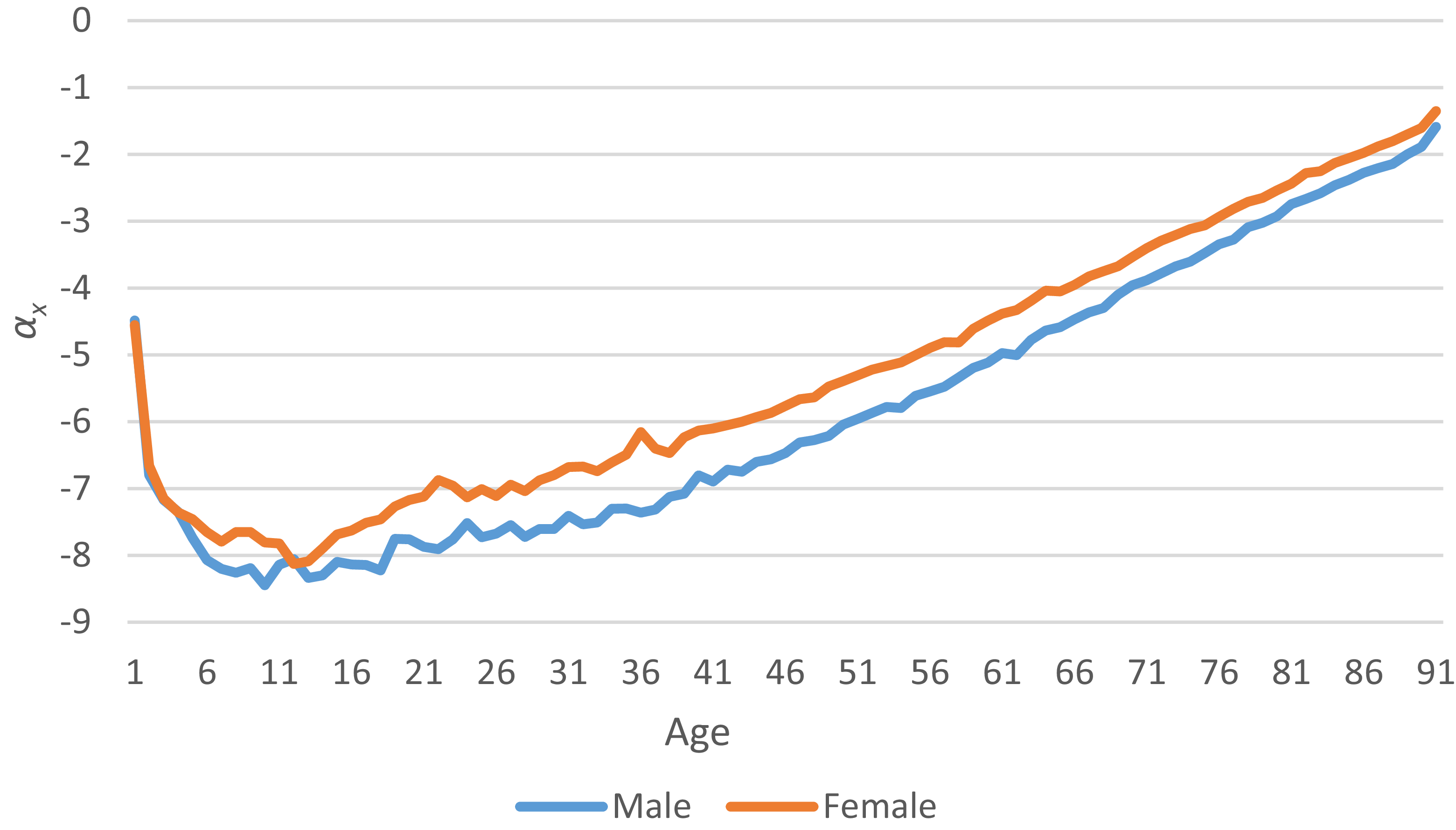
Figure 1 shows the age-time series of the estimated values αx for males and females in our country. The horizontal axis represents age. Figure 1 indicates that after a certain age, as age increases, the mortality rate continues to rise, and the rate for males is higher than for females, which is consistent with general expectations.

Figure 1. Age timing diagram of estimates α_x.

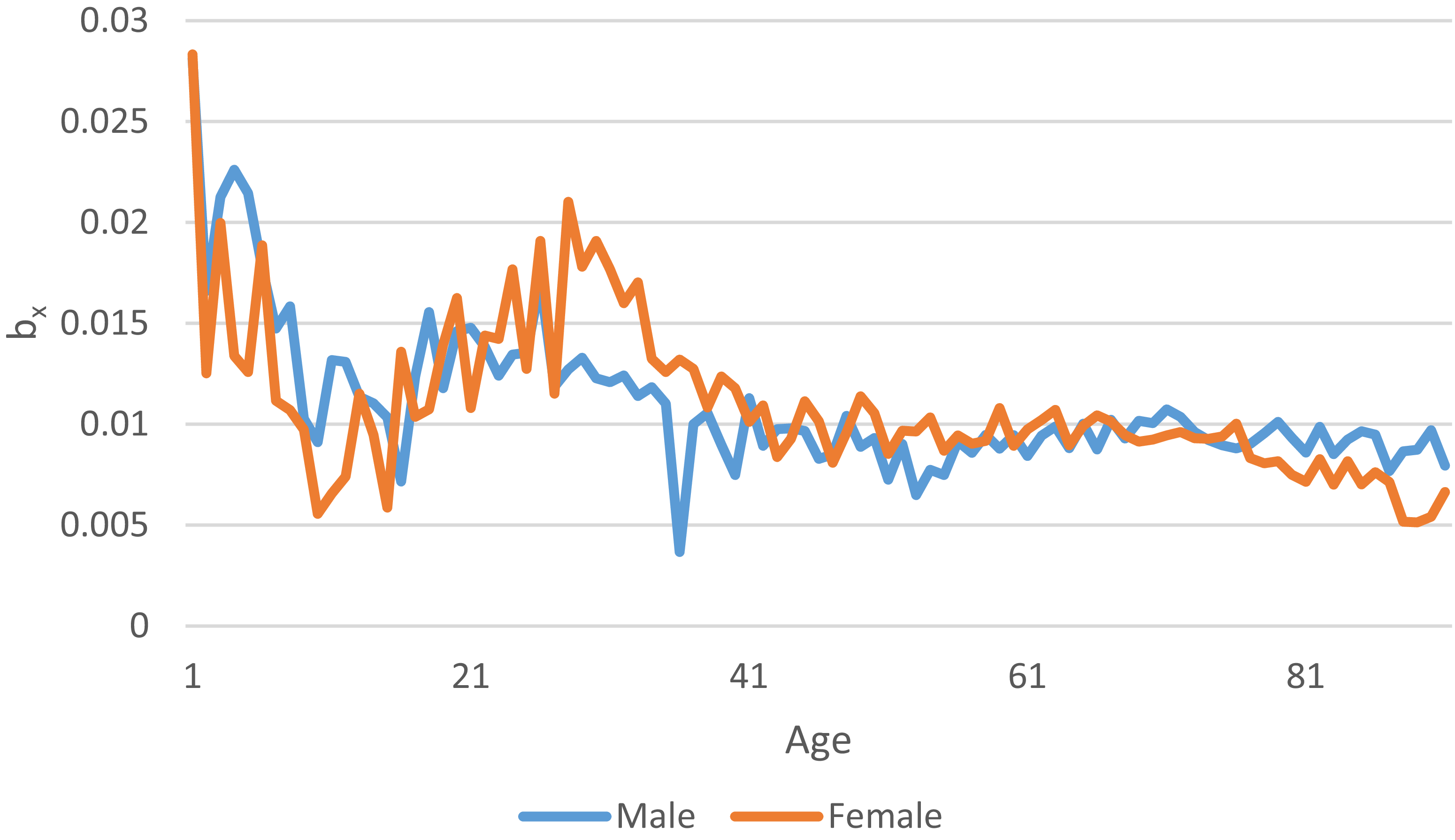
Figure 2 shows the age-time series of the estimated values $ {b}_{x}$ for males and females in our country. As previously described, $ {b}_{x}$ measures the sensitivity of $ {k}_{x}$ to age, meaning that as the value of $ {k}_{x}$ gradually decreases with age, $ {b}_{x}$ determines the rate at which the mortality rate for a specific age declines. As shown in the figure, in the age range of 0–60 years, the fluctuations in $ {b}_{x}$ are quite significant; but overall, there is a downward trend that gradually stabilises. This indicates that before the age of 60, mortality rate improvements are substantial, whereas after age 60, the rate of mortality improvement with age slows down.

Figure 2. Age timing diagram of estimates b _x.

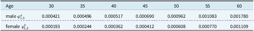
Then, according to the results of software analysis, the standard deviations of $ {k}_{t}^{A,2}$ , $ {k}_{t}^{A,1}$ , $ {k}_{t}^{L,2}$ and $ {k}_{t}^{L,1}$ are obtained (see Table 4), and their correlation matrix M is calculated:

$$M = \left[ {\matrix{ 1 & {0.8989} & {0.5521} & {0.4421} \cr {0.8989} & 1 & {0.7258} & {0.7420} \cr {0.5521} & {0.7258} & 1 & {0.9285} \cr {0.4421} & {0.7420} & {0.9285} & 1 \cr } } \right]$$

Table 4. Standard deviation of correlation parameter

Secondly, Cholesky decomposition refers to the fact that the real number term of the symmetric positive definite matrix M is the product of the lower triangular matrix and its transposed matrix, that is 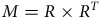$ M=R\times {R}^{T}$ . Hence, it can be obtained that R is expressed as follows:

$$R = \left( {\matrix{ 1 & 0 & 0 & 0 \cr {0.8989} & {0.4282} & 0 & 0 \cr {0.5221} & {0.5853} & {0.6204} & 0 \cr {0.4421} & {0.7864} & {0.3827} & {0.1991} \cr } } \right)$$

Using the lower triangular matrix, we obtain:

$$\left[ {\matrix{ {dZ_k^{A,2}\left( t \right)} \cr {dZ_k^{A,1}\left( t \right)} \cr {dZ_k^{L,2}\left( t \right)} \cr {dZ_k^{L,1}\left( t \right)} \cr } } \right] = \left[ {\matrix{ 1 & 0 & 0 & 0 \cr {0.8989} & {0.4382} & 0 & 0 \cr {0.5221} & {0.5853} & {0.6204} & 0 \cr {0.4421} & {0.7864} & {0.3827} & {0.1991} \cr } } \right] \times \left[ {\matrix{ {d{Z_{k1}}\left( t \right)} \cr {d{Z_{k2}}\left( t \right)} \cr {d{Z_{k3}}\left( t \right)} \cr {d{Z_{k4}}\left( t \right)} \cr } } \right]$$

The Cholesky decomposition coefficient between male and female life insurance and annuity obtained from the parameter estimation results is shown in the above formula, so that we can decompose the correlated Brownian motions $ {Z}_{k}^{A,2}$ , $ {Z}_{k}^{A,1}$ , $ {Z}_{k}^{L,2}$ and $ {Z}_{k}^{L,1}$ into four independent Brownian motion linear combinations $ {Z}_{k1}$ , $ {Z}_{k2}$ , $ {Z}_{k3,}$ and $ {Z}_{k4}$ . This transformation not only simplifies the model structure but also enables us to effectively identify the optimal insurance product portfolio that is minimally affected by longevity risk through variance minimisation.

4. Numerical Analysis

4.1. Basic Solution and Its Significance

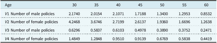
Considering only single-sex annuities within single-sex life insurance products simplifies the calculation of the total portfolio value V of a life insurance company and reduces the impact of mortality fluctuations on variance. The combined values V1 and V2 represent male annuities applied to male and female life insurance, respectively, while V3 and V4 represent female annuities applied to male and female life insurance, respectively, as expressed below:

$$ V1={N}_{x}^{A,1}\times V\left({m}_{x}^{A,1}\left(t\right)\right)+{N}_{x}^{L,1}\times V\left({m}_{x}^{L,1}\left(t\right)\right)$$

$$ V2={N}_{x}^{A,1}\times V\left({m}_{x}^{A,1}\left(t\right)\right)+{N}_{x}^{L,2}\times V\left({m}_{x}^{L,2}\left(t\right)\right)$$

$$ V3={N}_{x}^{A,2}\times V\left({m}_{x}^{A,2}\left(t\right)\right)+{N}_{x}^{L,1}\times V\left({m}_{x}^{L,1}\left(t\right)\right)$$

$$ V4={N}_{x}^{A,2}\times V\left({m}_{x}^{A,2}\left(t\right)\right)+{N}_{x}^{L,2}\times V\left({m}_{x}^{L,2}\left(t\right)\right)$$

The optimal solutions for hedging male annuities $ {N}_{x}^{L,1}$ and $ {N}_{x}^{L,2}$ are:

$$N_x^{L,2} = - {{({a_{31}}*{a_{21}} + {a_{32}}*{a_{22}})*{\varphi _{A,1}}} \over {{\varphi _{L,2}}*\mathop \sum \nolimits_{i = 1}^3{a_{3i}}^2}} = - M2*{{{\varphi _{A,1}}} \over {{\varphi _{L,2}}}}$$

$$N_x^{L,1} = - {{({a_{41}}*{a_{21}} + {a_{42}}*{a_{22}})*{\varphi _{A,1}}} \over {{\varphi _{L,1}}*\mathop \sum \nolimits_{i = 1}^4{a_{4i}}^2}} = - M1*{{{\varphi _{A,1}}} \over {{\varphi _{L,1}}}}$$

$$M1 = {{{a_{41}}*{a_{21}} + {a_{42}}*{a_{22}}} \over {\mathop \sum \nolimits_{i = 1}^4{a_{4i}}^2}},\quad M2 = {{{a_{31}}*{a_{21}} + {a_{32}}*{a_{22}}} \over {\mathop \sum \nolimits_{i = 1}^3{a_{3i}}^2}}$$

Similarly, the optimal solution for hedging female annuities is:

The expression for the optimal solution indicates that the number of life insurance policies required to hedge an annuity is influenced by two primary types of factors. The first factor is the correlation between the mortality risks of the portfolio products, which is determined by gender and age, and can be represented by the Cholesky decomposition coefficient. Ignoring the correlation of combined products, as noted in existing literature, will inevitably lead to erroneous results. The second factor is the sensitivity of hedging the product’s mortality risk, which primarily depends on the combined duration of the forces of mortality, denoted as $ {\varphi }_{L, 1}$ , $ {\varphi }_{L, 2}$ , $ {\varphi }_{L, 1}$ and $ {\varphi }_{L, 2}$ . The variation trends of these combined mortality durations across different ages and genders are shown in Table 5.

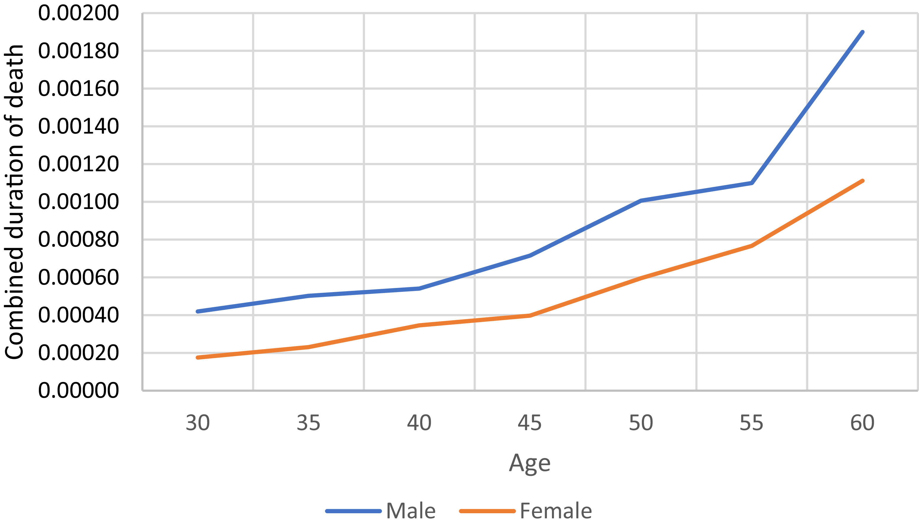
The results of the numerical simulation indicate that mortality rates for both males and females increase with age. From these results, the optimal insurance quantities $ {N}_{x}^{L,1}$ and $ {N}_{x}^{L,2}$ can be derived. The quantities of male and female annuity insurance (noting that all annuities referenced in this article pertain to whole life insurance) decrease with advancing age, a trend that is more clearly illustrated in the Figures 3, 4 and 5.

Figure 3. Combined duration of death.

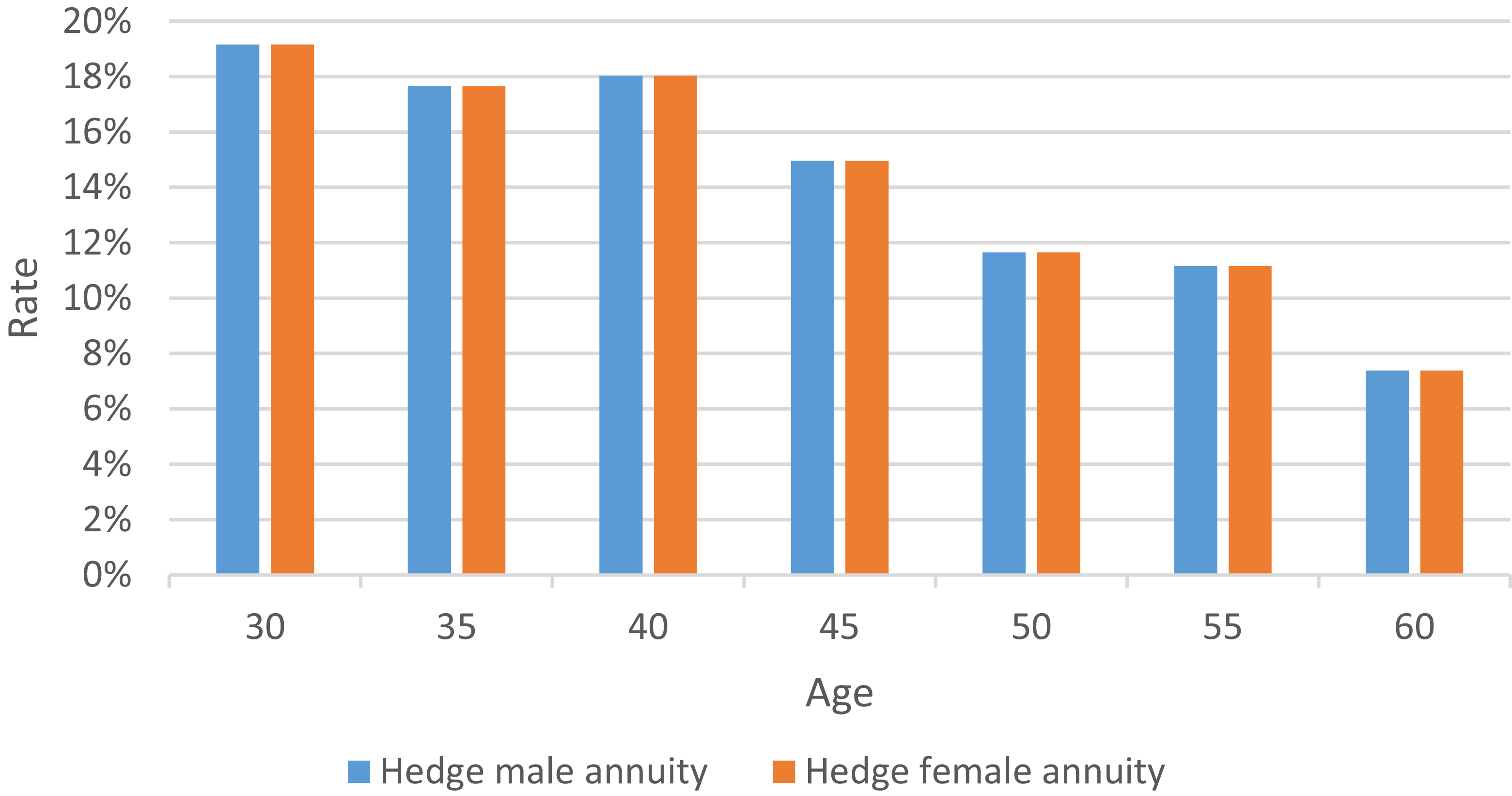
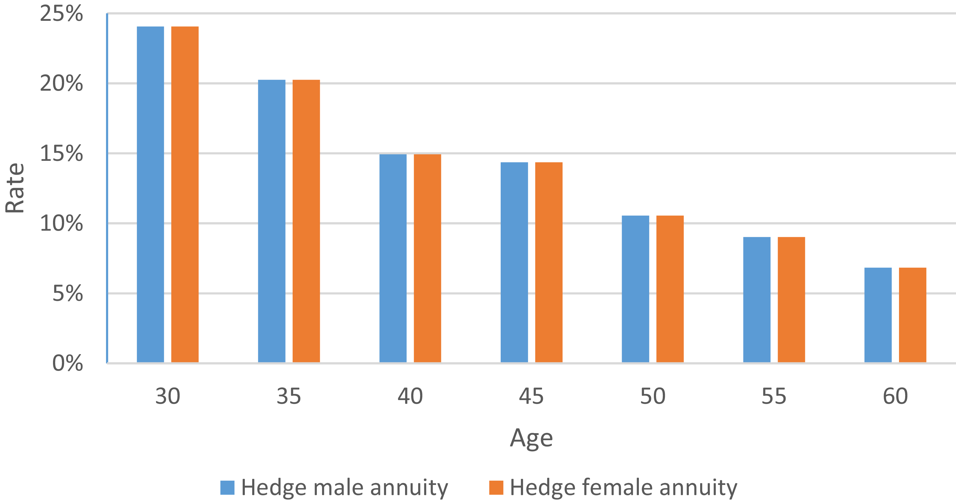
Figure 4. The number of life insurance policies needed to hedge male pension at various ages.

Figure 5. The number of life insurance policies needed to hedge female pension at various ages.

4.2. The Age of Men’s and Women’s Life Insurance Portfolio Ratio Characteristics

In order to facilitate the comparison of hedging results, we can calculate the number of life insurance policies equivalent to the annuities being hedged. Simply put, this involves calculating how many units of life insurance policies or combinations of policies are needed to hedge the longevity risk in one unit of annual annuity. That is, after considering the differences in the actuarial present values of whole life insurance and annuities, when we calculate the number of life insurance policies equivalent to male annuities for hedging, the required number of policies $ {\mathit{N}}_{\mathit{x}}^{\mathit{L},1}$ and $ {\mathit{N}}_{\mathit{x}}^{\mathit{L},2}$ becomes:

$$N_x^{L,1} = - {{({a_{41}}{{*}}\, {{{a}}_{{{21}}}}{{ + }}{{{a}}_{{{42}}}}{{*}}{{{a}}_{{{22}}}}){{*}}{\varphi _{{{A}},{{1}}}}{{*A}}_{{x}}^{{1}}} \over {\ddot a_x^1{{*}}{\varphi _{{{L}},{{1}}}}{{*}}\mathop \sum \nolimits_{{{i = 1}}}^{{4}}{{{a}}_{{{4i}}}}^{{2}}}} = - M1{{*}}{{{\varphi _{{{A}},{{1}}}}{{*A}}_{{x}}^{{1}}} \over {{{\ddot a}}_{{x}}^{{1}}{{*}}{\varphi _{{{L}},{{1}}}}}}$$

$$N_x^{L,2} = - {{({a_{31}}{{*}}\,{{{a}}_{{{21}}}}{{ + }}{{{a}}_{{{32}}}}{{*}}{{{a}}_{{{22}}}}){{*}}{\varphi _{{{A}},{{1}}}}{{*A}}_{{x}}^{{2}}} \over {\ddot a_x^1{{*}}{\varphi _{{{L}},{{2}}}}{{*}}\mathop \sum \nolimits_{{{i = 1}}}^{{3}}{{{a}}_{{{3i}}}}^{{2}}}} = - M2{{*}}{{{\varphi _{{{A}},{{1}}}}{{*A}}_{{x}}^{{2}}} \over {{{\ddot a}}_{{x}}^{{1}}{{*}}{\varphi _{{{L}},{{2}}}}}}$$

$ {\ddot{a}}_{x}$ is the actuarial present value of annuities, $ {A}_{x}$ is the actuarial present value of life insurance, and M is the combination of the Cholesky decomposition factors. The same is true for hedged female annuities. The specific results are shown in Tables 6 and 7.

When the immediate life annuity is transformed into a life annuity with an extension of n years, the expression for the number of hedging policies required changes to:

$$N_x^{L,1} = - M1{\rm{*}}{{{\varphi _{{{DA}},{\rm{1}}}}{{*A}}_{{x}}^{\rm{1}}} \over {{{n|}}{{{{\ddot a}}}_{{x}}}{\rm{*}}{\varphi _{{{L}},{{1}}}}}},{\it{N}}_{\it{x}}^{{\it{L}},{\rm{2}}}{\rm{ = - {\it M}2*}}{{{\varphi _{{{DA}},{\rm{1}}}}{{*A}}_{{x}}^{\rm{2}}} \over {{{n|}}{{{{\ddot a}}}_{\it{x}}}{\rm{*}}{\varphi _{{{L}},{{2}}}}}}$$

Where $ {\ddot{a}}_{x}$ is the immediate annuity, and $ {{n|}}{{\ddot a}}_{x}$ is the life annuity with a deferral of n years. $ {\varphi }_{DA,1}$ and $ {\varphi }_{A,1}$ are the mortality-adjusted durations of the deferred annuity and the immediate annuity, respectively. Let M1 denote a combination of coefficients derived from the Cholesky decomposition. Considering the hedging of male annuities as an example, we can observe that the proportion of life insurance for a male aged x within the combined male and female life insurance policies is expressed as follows:

(16) $${{M1 \times {A_x}} \over {\varphi _{L,1}^x}}/{\sum _{i = {\rm{1}},{\rm{2}}}}\left( {{{Mi \times A_x^i} \over {\varphi _{L,i}^x}}} \right) = {1 \over {1 + (M2/M1) \times (A_x^2/A_x^1) \times (\varphi _{L,1}^x/\varphi _{L,2}^x)}}$$

Based on the parameter characteristics of the ratio defined in Equation (16), the following conclusions can be drawn:

1. (1) As shown in the Equation (16), the resulting proportion does not involve any parameters related to annuities. This indicates that the proportion of life insurance used for hedging annuities is independent of annuity types and terms; it is determined solely by life insurance characteristics and the combinations across different ages. Consequently, whether dealing with an immediate or deferred annuity, the proportion remains the same for the same life insurance age. This conclusion is further demonstrated in Table 10.

2. (2) The results of (M2/M1) and $ \left({A}_{x}^{2}/{A}_{x}^{1}\right)$ all in the denominator are close to 1, while $ ({\varphi }_{L,1}^{x}/{\varphi }_{L,2}^{x})$ is greater than 1 as can be seen from Table 5, and there is a decreasing trend with the increase age. As shown in the Equation (16), it can be concluded that the proportion of male life insurance in the life insurance portfolio has an increasing trend with the increase of age. This conclusion is also reflected in the results in Table 8.

3. (3) From the formula for the life insurance policies required for each age group of males and females under the deferred annuity, it can be seen that the life insurance for a deferred annuity is affected by $ {\varphi }_{A,i}^{x}$ , with the number of policies decreasing with age; at the same time, $ {{n|}}{{\ddot a}}_{x}$ increases with the extension of the deferred period n. This trend can be more clearly observed in the three-dimensional graphs in Tables 8–11.

Table 5. Combined duration of death

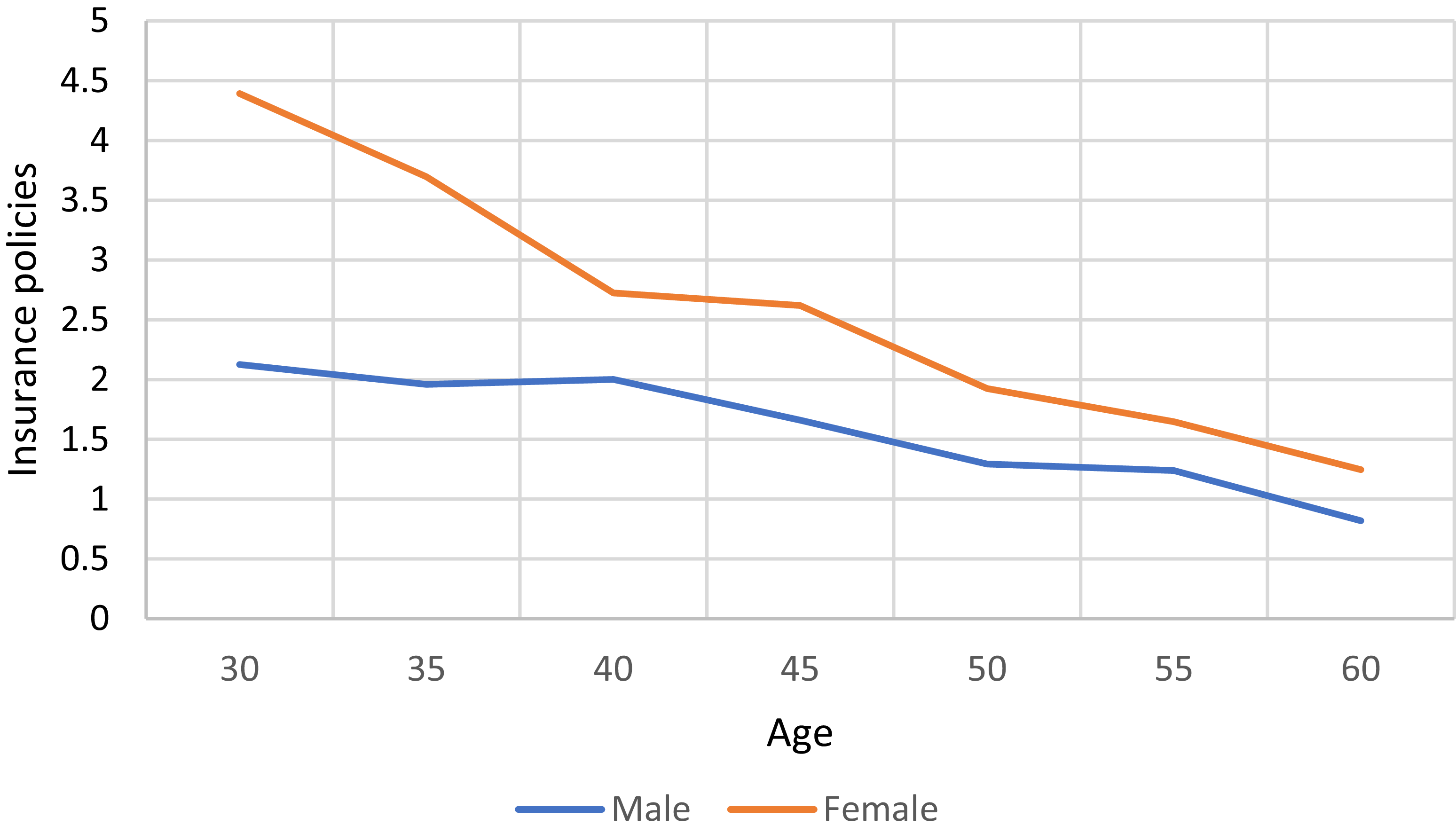
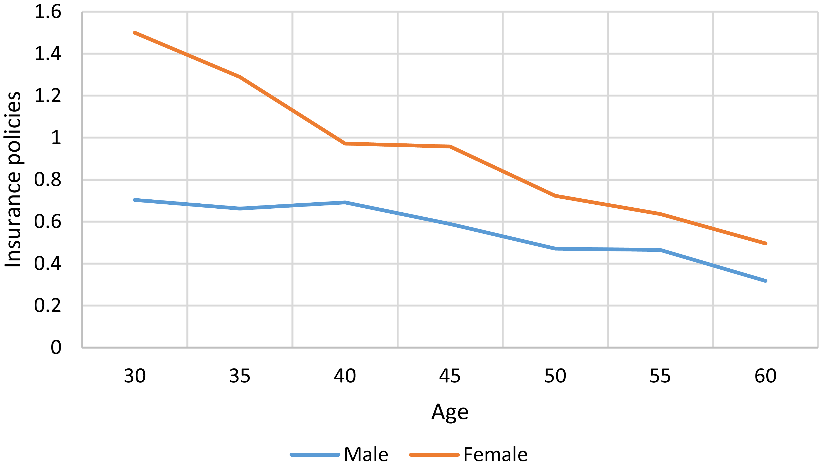
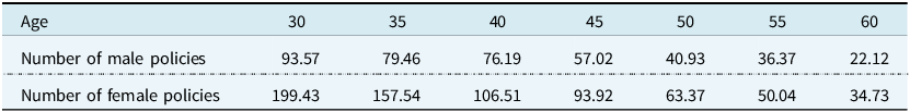
Table 6. Number of life insurance policies for men and women of all ages (hedged against 60-year-old male annuity)

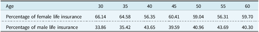
Table 7. Number of life insurance policies for men and women of all ages (hedged against 60-year-old female annuity)

Table 8. Percentage of life insurance policies required to hedge immediate/deferred annuities for 60-year-old women

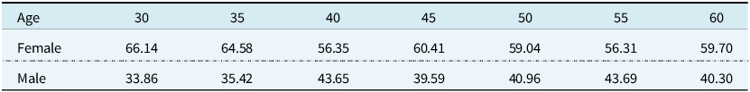
Table 9. Hedged annuity for 60-year-old males

Table 10. Hedging 60-year extended 10-year female annuity

Table 11. Hedging 60-year extended 10-year male annuity

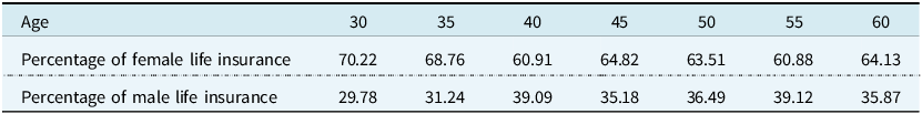
When considering the effect of a single-gender annuity on life insurance, we can determine the portfolio value for life insurance companies as well as the optimal results for male and female life insurance. When hedging male and female annuities, the proportion of male life insurance is notably lower than that of female life insurance. Furthermore, the proportion of male life insurance policies generally increases with age, whereas the proportion of female life insurance policies tends to decrease with age, as shown in the Tables 8 and 9.

For consistency and robustness in the study, we examine the hedging results of both male and female deferred annuities alongside immediate annuities for comparison. The age distribution for male and female life insurance portfolios required to minimise variance are presented:

Tables 8–11 shows that the proportion of life insurance policies at the same age remains constant, regardless of whether immediate or deferred annuities are used for hedging with the same life insurance policies. This result can be explained by the number of policy shares. For instance, for a male immediate annuity and a deferred annuity, the optimal male policy shares required – after converting the value of a life insurance policy to an annuity equivalent shown in Figures 6–9.

Figure 6. Female deferred annuity and male life insurance.

Figure 7. Male deferred annuity and female life insurance.

Figure 8. Female deferred annuity and female life insurance.

Figure 9. Male deferred annuity and male life insurance.

4.3. The Combination of a Single Gender Annuity and Life Insurance at Different Ages

In order to study the proportion of life insurance shares across different ages in the total combined portfolio when hedging annuity equivalents, as well as the differences in hedging effectiveness between genders, the hedging results are presented here.

To examine the proportion of life insurance shares across different ages within the total combined shares during hedging and to analyse the differences in hedging across genders, the hedging results are shown in Figures 10 and 11. This visualisation allows for a clearer observation of the varying age-based proportions when life insurance hedges male versus female annuities.

Figure 10. Proportion of male life insurance portfolios by age when hedging different gender annuities.

Figure 11. Proportion of female life insurance portfolios by age when hedging different gender annuities.

Referring to Figures 10 and 11, we can find that the proportion of male (or female) life insurance in the hedging portfolio is the same regardless of the male annuity or female annuity, and does not change with the change of gender. According to the previous expression of the optimal life insurance shares, it can be obtained that for each male life insurance portfolio equal to the male annuity, the number of male life insurance shares at the age of X should be:

(17) $$ - {{M \times {A_x} \times {\varphi _{A,1}}} \over {{\varphi _{L,1}}}}/{\sum _x}\left( { - {{M \times {A_x} \times {\varphi _{A,1}}} \over {{\varphi _{L,1}}}}} \right) = {{{A_x}/{\varphi _{L,1}}} \over {{\mathop \sum \nolimits_x}\left( {{A_x}/{\varphi _{L,1}}} \right)}}$$

M in the above formula is a function of the correlation coefficient a, whose form remains unchanged for different ages of the same sex, and $ {A}_{x}$ is the actuarial present value of whole life insurance at the age of x. Obviously, the $ {A}_{x}/{\varphi }_{L,1}^{x}$ in the above formula only depends on the fixed value of gender and age, so its proportion must also be fixed value. Hedging the annuity with different gender will not have an impact. Similarly, the same is true for the female annuity, i.e. the proportion of the same-age policies in the life insurance policy portfolio has no relationship with the gender of the hedged annuity policies and is a fixed value.

In order to study the combination of annuity policies of a single gender and age on male (female) life insurance policies of different ages and the different proportions of each age, the policy shares of life insurance policies of different ages were calculated, and the value of their life insurance combination was represented by V1–V4 above (see Table 12). At the same time, for the value of the male annuity in the mixed life insurance portfolio of men and women of different ages and the value of the female annuity in the mixed life insurance portfolio of men and women of different ages, V5 and V6 respectively, the expression is:

$$ V6={N}_{x}^{A,2}\times V\left({m}_{x}^{A,2}\left(t\right)\right)+\mathop \sum \limits_{i=\rm{1,2}}\mathop \sum \limits_{x}{N}_{x}^{L,i}\times V\left({m}_{x}^{L,i}\left(t\right)\right)$$

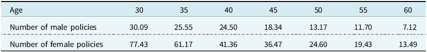
Table 12. Life insurance share of hedged annuities (Unit: copies)

For convenience of comparison, the following pie chart (Figures 12 and 13) is made up of the proportions of male and female life insurance policies in the V5 and V6 combinations in the whole life insurance portfolio. The main chart indicates the proportions of male and female life insurance policies in each age, and the sub-chart also shows the proportions of female life insurance policies in the whole female life insurance policies in each age.

Figure 12. Optimal Age Proportion of Male and Female Life Insurance for Hedging Male Annuities.

Figure 13. Optimal Age Proportion of Male and Female Life Insurance for Hedging Female Annuities.

4.4. Annuity and Life Insurance Hedging and Forecast Period Changes

The analysis in Section 4.3 is based on the forecast for the year 2023. To more comprehensively examine annuity and life insurance hedging from various perspectives, we extended the forecast period and generated trend charts depicting the required proportion of life insurance hedging for annuities across different ages, genders, and forecast years, as shown Figures 14–16 and 17.

Figure 14. Male annuity and female life insurance.

Figure 15. Male annuity and male life insurance.

Figure 16. Female annuity and male life insurance.

Figure 17. Female annuity and female life insurance.

Figures 14–17 illustrate that the life insurance hedging trends for different genders are opposite. For male life insurance hedging against male annuities, the required amount decreases as the forecast period lengthens, while for female life insurance hedging against male annuities, the required amount increases with a longer forecast period. Additionally, the trends in annuity and life insurance hedging for different genders align with the policy numbers in the forecast year.

5. Conclusions and Recommendations

5.1. Conclusion

In order to study the natural hedging strategy for effectively hedging longevity risk through a suitable proportion of life insurance and annuity product portfolio, given the insurance product portfolio containing annuities and life insurance policies of different ages and genders, this paper obtains the total value model of the product portfolio affected by mortality rate by using Ito’s lemma. It takes the minimisation of the variance of the value change of the product portfolio as the objective function, and numerically simulates the optimal product portfolio for hedging life insurance of male and female annuities under different structural parameters such as age, gender, duration, etc. The specific empirical method is to complete the estimation and prediction of mortality parameters, the calculation of mortality duration and convexity, and the calculation of the optimal product portfolio under the unified Bayesian MCMC framework. Through this research, the following conclusions are drawn:

1. (1) Regarding the theoretical foundation of natural hedging: Due to limitations in the statistical data on China’s population mortality rates, it is necessary to adapt and refine foreign mortality prediction methods to better fit the local context. Introducing the Bayesian MCMC framework yields satisfactory results in both the predicted mortality data and parameter simulations.

2. (2) In the empirical analysis of natural hedging strategies, examining combinations of annuity and life insurance policies reveals the following findings: (a) The optimal number of policy units varies by gender when using life insurance to hedge same-gender annuities, with a larger number of female policy units, and a higher proportion of both male and female life insurance portfolios hedging annuities; (b) When different types of annuities (e.g., deferred or immediate annuities) are hedged with the same life insurance policy, the proportion of life insurance policies remains constant, but the number of single-gender life insurance policies used to hedge annuities increases with the length of the deferral period; (c) When life insurance portfolios of different ages are used to hedge annuities, whether the annuities are male or female does not affect the proportion of life insurance units within the total portfolio for a given age group; (d) In later forecast years, fewer male life insurance policies and more female life insurance policies are required to hedge annuities.

Finally, this paper addresses the natural hedging problem across a broader product portfolio from a new perspective, providing practical insights for insurance companies in managing longevity risk. Although this study does not account for the effects of stochastic interest rates in the hedging of life insurance and annuity portfolios, estimating interest rate risk remains crucial in the current low-interest macroeconomic environment. Thus, analysing the combined effects of mortality fluctuations and interest rate changes on annuity and life insurance portfolios could yield more realistic results, warranting further research.

5.2. Relevant Recommendations

Firstly, longevity risk management should receive greater attention from life insurance companies. Longevity risk is not a short-term concern; it has long-term implications for the operation and sustainability of life insurance companies. Companies should proactively implement precautionary and strategic measures to address longevity risk, ensuring their long-term stability and growth.

Secondly, adjust the business structure to mitigate longevity risk and reinforce guarantees. Life insurance products with protective functions can offset the longevity risk posed by annuity products, thereby enhancing the management efficiency of longevity risk. Additionally, employing a natural hedging strategy can stimulate product research, development, and innovation within life insurance companies. By increasing the proportion of life insurance products in their portfolios, companies can not only manage longevity risk more effectively but also support a transformation in product structure, improve competitiveness, and contribute to the sustainable development of the entire insurance industry.

Thirdly, actively pursue product innovation to mitigate risks. Life insurance companies should foster a culture of innovation, encourage creative product design, develop relevant market segments, and provide diverse options for managing longevity risk. In practice, factors such as interest rates, age, and gender influence longevity risk and natural hedging strategies differently. Products tailored to different genders and age groups can also establish effective hedging relationships.