


1. Introduction
The distribution theory of sample spacings holds significant importance in diverse scientific areas. Many applications of spacings have been proposed in the literature related to reliability theory, randomness tests, goodness-of-fit tests, quality control, survival analysis, insurance claims, etc. For some early works on the subject, the interested reader may refer to [Reference Barton and David10, Reference Darling16, Reference Devroye17, Reference Weiss38]; we also refer to [Reference Arnold, Balakrishnan and Nagaraja1, Reference Pyke31] and the references therein. Inequalities and approximations for the distribution of ordered m-spacings have been proposed in [Reference Glaz20, Reference Glaz, Naus, Roos and Wallenstein22], while stochastic orderings on spacings were studied in [Reference Hu, Wang and Zhu23, Reference Kochar and Korwar24]. Moreover, [Reference Balakrishnan and Koutras5, Reference Glaz and Balakrishnan21] studied scan statistics using lowest uniform spacings. For more recent developments on spacings, including exact distributions of ordered spacings and asymptotic results, we refer to [Reference Bairamov, Berred and Stepanov4, Reference Balakrishnan, Nevzorov and Stepanov6, Reference Balakrishnan, Stepanov and Nevzorov7, Reference Berred and Stepanov12, Reference Berred and Stepanov13] and the references therein.
It is worth stressing that almost all the related literature concerns spacings on fixed-size samples from sequences of independent and identically distributed random variables that follow specific distributions, mostly uniform or exponential. In contrast, our aim is to study spacings that are generated from a sample of random size. This is in accordance with a remark in [Reference Pyke31] expressing interest in the question of distributions of spacings from random numbers of observations, e.g. when sampling from a renewal process. A similar idea has been applied and investigated in the case of order statistics, where the sample size is a non-negative integer-valued random variable, usually independent of the sample itself. Relating to this, for exact distributions and asymptotic results, we indicate the early works [Reference Barakat and El-Shandidy8, Reference Beirlant and Teugels11, Reference Epstein18, Reference Galambos19]. In addition, we refer to [Reference Silvestrov and Teugels34], which presented limit theorems for extremal processes with random sample size indexes (see also the references therein), and [Reference Silvestrov and Teugels35], which derived a number of limit theorems for max–sum processes with renewal stopping. For more recent developments, we mention [Reference Koutras and Koutras25] and the references therein.
The main purpose of this article is to study the minimal spacing when the size of the sample is random, a task which, to the best of our knowledge, has not yet been addressed. More specifically, we are interested in the exact and asymptotic distribution of the minimal spacing in a sequence of observations until a specific stopping rule applies, i.e. until a stopping time. In this manner, the size of the sample is not only random, but it also depends on the sample (and thus on the spacings). To treat this dependence problem, we apply an appropriate change of measure, which is related to a truncation of the distribution of the sample, under which the stopping time and the sample can now be considered independent. Exploiting this technique in Section 2, we initially prove a general result (Theorem 1) that provides a useful representation for the tail probability of the minimum observation until a general stopping time. In Section 3, we focus on a specific stopping time, i.e. the first time that the consecutive arrivals of a renewal process exceed a predefined time t. Employing the main outcome of Section 2, we provide an explicit formula for the distribution of the minimal spacing of the sample taken within this time interval (Theorem 2). In addition, we prove that this distribution is stochastically greater in the usual stochastic order than the distribution of the minimal spacing when the random size of the sample is assumed to be independent of the spacings (Theorem 3). For a comprehensive treatment on the subject of stochastic orders, including a variety of applications, we refer the reader to [Reference Shaked and Shanthikumar33]. Moreover, we propose upper and lower bounds for the distribution of the minimal spacing when the interarrival times of the renewal process possess the increasing failure rate (IFR) or decreasing failure rate (DFR) property. Furthermore, an exact formula, lower and upper bounds, and an asymptotic result for the survival function of the minimal spacing are obtained by assuming that the renewal process is a Poisson process. For the related problem of the longest gap in a Poisson process we refer to the recent works [Reference Asmussen, Ivanovs and Nielsen2, Reference Asmussen, Ivanovs and Segers3, Reference Omwonylee29, Reference Omwonylee and Yang30] and the references therein. We further derive results for the distribution of the minimal spacing when the interarrival times follow other specific distributions (Erlang and uniform). In Section 4, we illustrate the applicability of our theoretical results by presenting several numerical comparisons among the exact distribution formulae for the distribution of the minimal spacing, the proposed bounds, and the approximations of Section 3. Finally, in Section 5, we briefly discuss three possible applications of our main results in reliability theory, quality control, and hypothesis testing.
2. The distribution of the minimum observation until a stopping time
In a probability space
 $(\Omega,{\mathcal A},\mathbb{P})$
, let
$(\Omega,{\mathcal A},\mathbb{P})$
, let
 $X_{1},X_{2},\ldots$
be a sequence of independent and identically distributed (i.i.d.) random variables (RVs) with common cumulative distribution function (CDF) F. Moreover, consider an almost surely (a.s.) finite stopping time
$X_{1},X_{2},\ldots$
be a sequence of independent and identically distributed (i.i.d.) random variables (RVs) with common cumulative distribution function (CDF) F. Moreover, consider an almost surely (a.s.) finite stopping time
 $T\in\{1,2,\ldots\}$
associated with this sequence. Remember that a discrete RV
$T\in\{1,2,\ldots\}$
associated with this sequence. Remember that a discrete RV
 $T\in\{1,2,\ldots\}$
is a stopping time with respect to
$T\in\{1,2,\ldots\}$
is a stopping time with respect to
 $X_{1},X_{2},\ldots$
when, for every
$X_{1},X_{2},\ldots$
when, for every
 $k\in\{1,2,\ldots\}$
, the event
$k\in\{1,2,\ldots\}$
, the event
 $[T=k]$
depends only on
$[T=k]$
depends only on
 $X_{1},X_{2},\ldots,X_{k}$
(i.e. it is independent of
$X_{1},X_{2},\ldots,X_{k}$
(i.e. it is independent of
 $X_{k+1},X_{k+2},\ldots$
). This implies that the indicator RV
$X_{k+1},X_{k+2},\ldots$
). This implies that the indicator RV
 $\boldsymbol{1}_{[T\leq k]}$
is a function of
$\boldsymbol{1}_{[T\leq k]}$
is a function of
 $X_{1},X_{2},\ldots,X_{k}$
, i.e.
$X_{1},X_{2},\ldots,X_{k}$
, i.e.
 $\boldsymbol{1}_{[T\leq k]}=g_{k}(X_{1},X_{2},\ldots,X_{k})$
for some measurable function
$\boldsymbol{1}_{[T\leq k]}=g_{k}(X_{1},X_{2},\ldots,X_{k})$
for some measurable function
 $g_{k}$
. We are interested in the distribution of the minimum RV
$g_{k}$
. We are interested in the distribution of the minimum RV
 $M_{T}\;:\!=\;\min\{X_{1},X_{2},\ldots,X_{T}\}$
. Note that this distribution cannot be easily found by conditioning on the stopping time T because, in general, the
$M_{T}\;:\!=\;\min\{X_{1},X_{2},\ldots,X_{T}\}$
. Note that this distribution cannot be easily found by conditioning on the stopping time T because, in general, the
 $X_{i}$
are not independent of T.
$X_{i}$
are not independent of T.
In the same measurable space
 $(\Omega,{\mathcal A})$
, for
$(\Omega,{\mathcal A})$
, for
 $w\in\mathbb{R}$
such that
$w\in\mathbb{R}$
such that
 $F(w)<1$
, we also consider a probability measure
$F(w)<1$
, we also consider a probability measure
 $\mathbb{P}_{w}$
such that
$\mathbb{P}_{w}$
such that
 $\mathbb{P}_{w}(A)\;:\!=\;\mathbb{E}\big(\boldsymbol{1}_{A}\varDelta_{n}^{w}\big)$
for every
$\mathbb{P}_{w}(A)\;:\!=\;\mathbb{E}\big(\boldsymbol{1}_{A}\varDelta_{n}^{w}\big)$
for every
 $A\in\mathcal{A}_{n}=\sigma(X_{1},\ldots,X_{n})$
,
$A\in\mathcal{A}_{n}=\sigma(X_{1},\ldots,X_{n})$
,
 $n=1,2,\ldots$
, where
$n=1,2,\ldots$
, where
 \begin{align*}\varDelta_{n}^{w}\;:\!=\;\prod_{i=1}^{n}\frac{\boldsymbol{1}_{[X_{i}>w]}}{1-F(w)},\quad n=1,2,\ldots\end{align*}
is a martingale with respect to the filtration
 $\mathcal{A}_{n}$
,
$\mathcal{A}_{n}$
,
 $n=1,2,\ldots$
. Then, the RVs
$n=1,2,\ldots$
. Then, the RVs
 $X_{1},X_{2},\ldots$
are again i.i.d. under the w-truncated probability measure
$X_{1},X_{2},\ldots$
are again i.i.d. under the w-truncated probability measure
 $\mathbb{P}_{w}$
, and each of them has the following w-truncated CDF
$\mathbb{P}_{w}$
, and each of them has the following w-truncated CDF
 $F_{w}$
:
$F_{w}$
:
 \begin{align} F_{w}(x) & \;:\!=\; \mathbb{P}_{w}(X_{n}\leq x) \nonumber \\ & = \mathbb{E}\big(\boldsymbol{1}_{[X_{n}\leq x]}\varDelta_{n}^{w}\big) = \mathbb{E}\bigg(\boldsymbol{1}_{[X_{n}\leq x]}\frac{\boldsymbol{1}_{[X_{n}>w]}}{1-F(w)}\bigg) = \frac{F(x)-F(w)}{1-F(w)}\boldsymbol{1}_{[x>w]}, \end{align}
since
 $X_1,X_2,\ldots,X_n$
are independent and
$X_1,X_2,\ldots,X_n$
are independent and
 $\mathbb{E}(\varDelta_{n}^{w})=1$
for all
$\mathbb{E}(\varDelta_{n}^{w})=1$
for all
 $n=1,2,\ldots$
and
$n=1,2,\ldots$
and
 $w\in\mathbb{R}$
with
$w\in\mathbb{R}$
with
 $F(w)<1$
.
$F(w)<1$
.
In what follows, we shall denote by
 $\mathbb{E}_{w}$
the expectation under
$\mathbb{E}_{w}$
the expectation under
 $\mathbb{P}_{w}$
. So, under the above setup, we derive the following lemma.
$\mathbb{P}_{w}$
. So, under the above setup, we derive the following lemma.
Lemma 1. For any real measurable function h in
 $\mathbb{R}^{k}$
,
$\mathbb{R}^{k}$
,
 $k\geq1$
, and
$k\geq1$
, and
 $w\in\mathbb{R}$
such that
$w\in\mathbb{R}$
such that
 $F(w)<1$
,
$F(w)<1$
,
 \begin{align*} \mathbb{E}_{w}(h(X_{1},\ldots,X_{k})) = \frac{\mathbb{E}\big(\boldsymbol{1}_{[\!\min\{X_{1},X_{2},\ldots,X_{k}\}>w]}\,h(X_{1},\ldots,X_{k})\big)}{(1-F(w))^{k}}, \end{align*}
where
 $\mathbb{E}$
,
$\mathbb{E}$
,
 $\mathbb{E}_{w}$
denote the expectations under the probability measures
$\mathbb{E}_{w}$
denote the expectations under the probability measures
 $\mathbb{P}$
,
$\mathbb{P}$
,
 $\mathbb{P}_{w}$
, respectively.
$\mathbb{P}_{w}$
, respectively.
Proof. Invoking the independence of
 $X_{1},\ldots,X_{k}$
in combination with (1), we have, for any measurable function h,
$X_{1},\ldots,X_{k}$
in combination with (1), we have, for any measurable function h,
 \begin{align*} \mathbb{E}_{w}(h(X_{1},\ldots,X_{k})) & = \int\cdots\int h(x_{1},\ldots,x_{k})\,{\mathrm{d}} F_{w}(x_{1}) \cdots {\mathrm{d}} F_{w}(x_{k}) \\ & = \int\cdots\int h(x_{1},\ldots,x_{k}) \frac{\boldsymbol{1}_{[x_{1}>w]}\cdots\boldsymbol{1}_{[x_{k}>w]}}{(1-F(w))^{k}}\,{\mathrm{d}} F(x_{1})\cdots{\mathrm{d}} F(x_{k}) \\ & = \frac{\mathbb{E}\big(\boldsymbol{1}_{[\!\min\{X_{1},X_{2},\ldots,X_{k}\}>w]}\,h(X_{1},\ldots,X_{k})\big)} {(1-F(w))^{k}}. \end{align*}
Now, the distribution of
 $M_{T}=\min\{X_{1},X_{2},\ldots,X_{T}\}$
may be obtained by exploiting the previous lemma, as shown in the result that follows.
$M_{T}=\min\{X_{1},X_{2},\ldots,X_{T}\}$
may be obtained by exploiting the previous lemma, as shown in the result that follows.
Theorem 1. Let T be an a.s. finite stopping time associated with a sequence of i.i.d. RVs
 $X_{1},X_{2},\ldots$
with common CDF F. If
$X_{1},X_{2},\ldots$
with common CDF F. If
 $M_{T}=\min\{X_{1},X_{2},\ldots,X_{T}\}$
then
$M_{T}=\min\{X_{1},X_{2},\ldots,X_{T}\}$
then
 \begin{align*} \mathbb{P}(M_{T}>w) = \mathbb{E}_{w}\big((1-F(w))^{T}\big) \end{align*}
for
 $w\in\mathbb{R}$
such that
$w\in\mathbb{R}$
such that
 $F(w)<1$
.
$F(w)<1$
.
Proof. Since we have assumed that
 $P(T<\infty)=1$
, we have
$P(T<\infty)=1$
, we have
 \begin{align*} \mathbb{P}(M_{T}>w) = \sum_{k=1}^{\infty}\mathbb{P}(M_{T}>w,T=k) & = \sum_{k=1}^{\infty}\mathbb{E}\big(\boldsymbol{1}_{[T=k]}\boldsymbol{1}_{[M_{T}>w]}\big) \\ & = \sum_{k=1}^{\infty}\mathbb{E}\big(\boldsymbol{1}_{[T=k]}\boldsymbol{1}_{[\!\min\{X_{1},X_{2},\ldots,X_{k}\}>w]}\big) \\ & = \sum_{k=1}^{\infty}(1-F(w))^{k}\mathbb{E}_{w}\big(\boldsymbol{1}_{[T=k]}\big) \\ & = \sum_{k=1}^{\infty}(1-F(w))^{k}\mathbb{P}_{w}(T=k) = \mathbb{E}_{w}\big((1-F(w))^{T}\big), \end{align*}
where the fourth equality follows from a direct application of Lemma 1.
It is worth pointing out that Lemma 1 and Theorem 1 do not rely on the existence of a density for the RVs
 $X_{1},X_{2},\ldots$
Furthermore, it should be noted that Theorem 1 is valid generally for every stopping time under the above assumptions. However, in the rest of this paper we shall be mainly concerned with a specific type of stopping time associated with the number of arrivals in a renewal process in a given time interval. Applications considering other types of stopping times will be the purpose of subsequent work.
$X_{1},X_{2},\ldots$
Furthermore, it should be noted that Theorem 1 is valid generally for every stopping time under the above assumptions. However, in the rest of this paper we shall be mainly concerned with a specific type of stopping time associated with the number of arrivals in a renewal process in a given time interval. Applications considering other types of stopping times will be the purpose of subsequent work.
3. The distribution of the minimal spacing in a renewal process
Under the setup of Section 2, we assume that the i.i.d. RVs
 $X_{1},X_{2},\ldots$
are the interarrival times of a renewal process
$X_{1},X_{2},\ldots$
are the interarrival times of a renewal process
 $\{Y_{t},t\geq0\}$
, i.e.
$\{Y_{t},t\geq0\}$
, i.e.
 $Y_{t}=\sup\{i\geq1\colon X_{1}+\cdots+X_{i}\leq t\}$
. Moreover, we set
$Y_{t}=\sup\{i\geq1\colon X_{1}+\cdots+X_{i}\leq t\}$
. Moreover, we set
 $T\;:\!=\;Y_{t}+1$
. Then T is the number of summands until the sum of the
$T\;:\!=\;Y_{t}+1$
. Then T is the number of summands until the sum of the
 $X_{i}$
exceeds t for the first time. Also, the event
$X_{i}$
exceeds t for the first time. Also, the event
 $[Y_{t}+1=k]$
depends only on
$[Y_{t}+1=k]$
depends only on
 $X_{1},X_{2},\ldots,X_{k}$
, and therefore T is a stopping time associated with the sequence
$X_{1},X_{2},\ldots,X_{k}$
, and therefore T is a stopping time associated with the sequence
 $X_{1},X_{2},\ldots$
. Thus, the RV
$X_{1},X_{2},\ldots$
. Thus, the RV
 $M_{T}\;:\!=\;\min\{X_{1},X_{2},\ldots,X_{T}\}=\min\{X_{1},X_{2},\ldots,X_{Y_{t}+1}\}$
will now denote the minimal spacing that starts in the interval [0, t]. Here, notice that if
$M_{T}\;:\!=\;\min\{X_{1},X_{2},\ldots,X_{T}\}=\min\{X_{1},X_{2},\ldots,X_{Y_{t}+1}\}$
will now denote the minimal spacing that starts in the interval [0, t]. Here, notice that if
 $S_{k}\;:\!=\;X_{1}+\cdots+X_{k}$
,
$S_{k}\;:\!=\;X_{1}+\cdots+X_{k}$
,
 $k=1,2,\ldots$
, is the kth arrival epoch of the renewal process
$k=1,2,\ldots$
, is the kth arrival epoch of the renewal process
 $\{Y_{t},t\geq0\}$
, then the last spacing may extend beyond t because
$\{Y_{t},t\geq0\}$
, then the last spacing may extend beyond t because
 $S_{Y_{t}}\leq t$
and
$S_{Y_{t}}\leq t$
and
 $S_{Y_{t}+1}\geq t$
.
$S_{Y_{t}+1}\geq t$
.
Throughout the rest of this paper, since T is a function of t, the minimal spacing will be denoted by
 $D_{t}$
instead of
$D_{t}$
instead of
 $M_{T}$
to emphasize its dependence on time t. Notice also that the truncated measure
$M_{T}$
to emphasize its dependence on time t. Notice also that the truncated measure
 $\mathbb{P}_{w}$
will be meaningfully defined only for
$\mathbb{P}_{w}$
will be meaningfully defined only for
 $w\geq0$
such that
$w\geq0$
such that
 $F(w)<1$
since the RVs
$F(w)<1$
since the RVs
 $X_{1},X_{2},\ldots$
will be non-negative (also with finite expectation) as being the interarrival times of a renewal process.
$X_{1},X_{2},\ldots$
will be non-negative (also with finite expectation) as being the interarrival times of a renewal process.
The next result provides a general expression for the distribution of the minimal spacing
 $D_{t}$
in a renewal process.
$D_{t}$
in a renewal process.
Theorem 2. Let
 $D_{t}=\min\{X_{1},X_{2},\ldots,X_{T}\}$
be the minimal spacing that starts in the time interval [0, t] in a counting renewal process
$D_{t}=\min\{X_{1},X_{2},\ldots,X_{T}\}$
be the minimal spacing that starts in the time interval [0, t] in a counting renewal process
 $\{Y_{t},t\geq0\}$
, where
$\{Y_{t},t\geq0\}$
, where
 $T=Y_{t}+1$
and
$T=Y_{t}+1$
and
 $X_{1},X_{2},\ldots$
are the interarrival spacings between successive appearances of events with common CDF F. Then
$X_{1},X_{2},\ldots$
are the interarrival spacings between successive appearances of events with common CDF F. Then
 \begin{equation*} \mathbb{P}(D_{t} > w) = \begin{cases} {\displaystyle F(w)\sum_{k=1}^{\infty}(1-F(w))^{k}\big(1-F_{w}^{*k}(t)\big),} & 0 < w < t, \\ 1-F(w), & w\geq t, \end{cases} \end{equation*}
where
 $S_{k}=\sum_{i=1}^{k}X_{i}$
and
$S_{k}=\sum_{i=1}^{k}X_{i}$
and
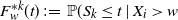 $F_{w}^{*k}(t) \;:\!=\; \mathbb{P}(S_{k}\leq t \mid X_{i}>w$
for all
$F_{w}^{*k}(t) \;:\!=\; \mathbb{P}(S_{k}\leq t \mid X_{i}>w$
for all
 $i=1,\ldots,k)$
denotes the CDF of the kth-order convolution of the w-truncated F.
$i=1,\ldots,k)$
denotes the CDF of the kth-order convolution of the w-truncated F.
Proof. Applying Theorem 1, we get
 \begin{align*} \mathbb{P}(D_{t} > w) & = \mathbb{E}_{w}\big((1-F(w))^{T}\big) \\ & = \sum_{k=1}^{\infty}(1-F(w))^{k}\,\mathbb{P}_{w}(T=k) \\ & = \sum_{k=1}^{\infty}(1-F(w))^{k}\,\mathbb{P}_{w}(T\leq k) - \sum_{k=2}^{\infty}(1-F(w))^{k}\,\mathbb{P}_{w}(T\leq k-1) \\ & = \sum_{k=1}^{\infty}(1-F(w))^{k}\,\mathbb{P}_{w}(T\leq k) - \sum_{k=1}^{\infty}(1-F(w))^{k+1}\mathbb{P}_{w}(T\leq k) \\ & = F(w)\sum_{k=1}^{\infty}(1-F(w))^{k}\,\mathbb{P}_{w}(T\leq k) \end{align*}
(obviously,
 $\mathbb{P}_{w}(T\leq0)=0$
), and taking into account that
$\mathbb{P}_{w}(T\leq0)=0$
), and taking into account that
 $[Y_{t}\leq k-1]=[S_{k}>t]$
, we finally obtain that
$[Y_{t}\leq k-1]=[S_{k}>t]$
, we finally obtain that
 \begin{equation*} \mathbb{P}_{w}(T\leq k) = \mathbb{P}_{w}(Y_{t}\leq k-1) = \mathbb{P}_{w}(S_{k}>t) = \mathbb{P}(S_{k}>t \mid X_{i}>w\ \text{for all}\ i=1,\ldots,k). \end{equation*}
Notice that
 $\mathbb{P}(S_{k}>t \mid X_{i}>w\ \text{for all}\ i=1,\ldots,k)=1$
when
$\mathbb{P}(S_{k}>t \mid X_{i}>w\ \text{for all}\ i=1,\ldots,k)=1$
when
 $t\leq w$
, which in this case yields
$t\leq w$
, which in this case yields
 \begin{align*} \mathbb{P}(D_{t} > w) = F(w)\sum_{k=1}^{\infty}(1-F(w))^{k}=1-F(w), \end{align*}
and the proof is completed.
Clearly, in order to find a more explicit formula for
 $\mathbb{P}(D_{t} > w)$
by Theorem 2, we should have at hand the exact distribution of the arrival epochs
$\mathbb{P}(D_{t} > w)$
by Theorem 2, we should have at hand the exact distribution of the arrival epochs
 $S_{k}$
. As we will see in Proposition 1, if we consider a Poisson process then an exact formula for
$S_{k}$
. As we will see in Proposition 1, if we consider a Poisson process then an exact formula for
 $\mathbb{P}(D_{t} > w)$
can be derived by this result.
$\mathbb{P}(D_{t} > w)$
can be derived by this result.
Remark 1. It may also be of interest to study the distribution of
 $C_{t}\;:\!=\;\min\{X_{1},X_{2},\ldots,X_{Y_{t}}\}$
. This RV does not take into account the value of the last interarrival time that starts at
$C_{t}\;:\!=\;\min\{X_{1},X_{2},\ldots,X_{Y_{t}}\}$
. This RV does not take into account the value of the last interarrival time that starts at
 $S_{Y_{t}}\in[0,t]$
, but its main drawback is that
$S_{Y_{t}}\in[0,t]$
, but its main drawback is that
 $Y_{t}$
is not a stopping time (i.e.
$Y_{t}$
is not a stopping time (i.e.
 $[Y_{t}=n]\notin\sigma(X_{1},\ldots,X_{n})$
), and therefore we cannot directly employ our general methodology based on stopping times (cf. Theorem 1). However, it is obvious that
$[Y_{t}=n]\notin\sigma(X_{1},\ldots,X_{n})$
), and therefore we cannot directly employ our general methodology based on stopping times (cf. Theorem 1). However, it is obvious that
 $D_{t}\leq C_{t}$
, and thus
$D_{t}\leq C_{t}$
, and thus
 $\mathbb{P}(D_{t} > w)\leq\mathbb{P}(C_{t} > w)$
,
$\mathbb{P}(D_{t} > w)\leq\mathbb{P}(C_{t} > w)$
,
 $w>0$
; the latter inequality implies that
$w>0$
; the latter inequality implies that
 $C_{t}$
is stochastically larger than
$C_{t}$
is stochastically larger than
 $D_{t}$
, see Definition 1. Hence, the result of Theorem 2 and all the lower bounds for the probability
$D_{t}$
, see Definition 1. Hence, the result of Theorem 2 and all the lower bounds for the probability
 $\mathbb{P}(D_{t} > w)$
to be presented in this work will serve as lower bounds for the probability
$\mathbb{P}(D_{t} > w)$
to be presented in this work will serve as lower bounds for the probability
 $\mathbb{P}(C_{t} > w)$
as well.
$\mathbb{P}(C_{t} > w)$
as well.
Next, aside from the above-mentioned (dependent on the
 $X_{i}$
) renewal process
$X_{i}$
) renewal process
 $\{Y_{t},t\geq0\}$
, we also consider another renewal process
$\{Y_{t},t\geq0\}$
, we also consider another renewal process
 $\{K_{t},t\geq0\}$
with
$\{K_{t},t\geq0\}$
with
 $K_{t}=_{{\mathrm{st}}}Y_{t}$
for all
$K_{t}=_{{\mathrm{st}}}Y_{t}$
for all
 $t\geq0$
, where ‘
$t\geq0$
, where ‘
 $=_{{\mathrm{st}}}$
’ denotes equality in distribution. In addition, the process
$=_{{\mathrm{st}}}$
’ denotes equality in distribution. In addition, the process
 $\{K_{t},t\geq0\}$
is assumed to be independent of the
$\{K_{t},t\geq0\}$
is assumed to be independent of the
 $X_{i}$
. If
$X_{i}$
. If
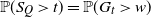
 $G_{t}\;:\!=\;\min\{X_{1},X_{2},\ldots,X_{K_{t}+1}\}$
, then we shall prove that the minimal spacing
$G_{t}\;:\!=\;\min\{X_{1},X_{2},\ldots,X_{K_{t}+1}\}$
, then we shall prove that the minimal spacing
 $D_{t}$
is larger stochastically than
$D_{t}$
is larger stochastically than
 $G_{t}$
with respect to the usual stochastic ordering (cf. [Reference Shaked and Shanthikumar33, Reference Szekli36]).
$G_{t}$
with respect to the usual stochastic ordering (cf. [Reference Shaked and Shanthikumar33, Reference Szekli36]).
Definition 1. An RV X is smaller than an RV Y in the usual stochastic order, written
 $X\preceq_{{\mathrm{st}}}Y$
, if and only if
$X\preceq_{{\mathrm{st}}}Y$
, if and only if
 $\mathbb{P}(X > u)\leq\mathbb{P}(Y > u)$
for all
$\mathbb{P}(X > u)\leq\mathbb{P}(Y > u)$
for all
 $u\in\mathbb{R}$
.
$u\in\mathbb{R}$
.
We then obtain the following result, which implies that, when the dependence between the spacings and the stopping time is ignored, we get a stochastically smaller minimum spacing.
Theorem 3. Let
 $D_{t}=\min\{X_{1},X_{2},\ldots,X_{Y_{t}+1}\}$
be the minimal spacing that starts in the time interval [0, t] in a renewal process
$D_{t}=\min\{X_{1},X_{2},\ldots,X_{Y_{t}+1}\}$
be the minimal spacing that starts in the time interval [0, t] in a renewal process
 $\{Y_{t},t\geq0\}$
, and
$\{Y_{t},t\geq0\}$
, and
 $X_{1},X_{2},\ldots$
the interarrival times (spacings) between successive appearances of events. Moreover, consider another renewal process
$X_{1},X_{2},\ldots$
the interarrival times (spacings) between successive appearances of events. Moreover, consider another renewal process
 $\{K_{t},t\geq0\}$
with
$\{K_{t},t\geq0\}$
with
 $K_{t}=_{{\mathrm{st}}}Y_{t}$
that is independent of the
$K_{t}=_{{\mathrm{st}}}Y_{t}$
that is independent of the
 $X_{i}$
. If
$X_{i}$
. If
 $G_{t}=\min\{X_{1},X_{2},\ldots,X_{K_{t}+1}\}$
, then
$G_{t}=\min\{X_{1},X_{2},\ldots,X_{K_{t}+1}\}$
, then
 $G_{t}\preceq_{{\mathrm{st}}}D_{t}$
, i.e.
$G_{t}\preceq_{{\mathrm{st}}}D_{t}$
, i.e.
 $D_{t}$
is larger than
$D_{t}$
is larger than
 $G_{t}$
with respect to the usual stochastic order.
$G_{t}$
with respect to the usual stochastic order.
Proof. Theorem 2 yields, for
 $w>0$
,
$w>0$
,
 \begin{align} \mathbb{P}(D_{t} > w) & = F(w)\sum_{k=1}^{\infty}(1-F(w))^{k}\, \mathbb{P}(S_{k} > t \mid X_{i} > w\ \text{for all}\ i=1,\ldots,k) \nonumber \\ & = F(w)\sum_{k=1}^{\infty}(1-F(w))^{k}\, \mathbb{P}(S_{k} > t \mid \min\{X_{1},\ldots,X_{k}\} > w) \end{align}
(it can be easily seen that the previous formula includes both cases
 $0 < w < t$
and
$0 < w < t$
and
 $w\geq t$
, which are stated separately in the aforementioned theorem). Exploiting the fact that
$w\geq t$
, which are stated separately in the aforementioned theorem). Exploiting the fact that
 $S_{k}=\sum_{i=1}^{k}X_{i}$
and
$S_{k}=\sum_{i=1}^{k}X_{i}$
and
 $(X_{1},\ldots,X_{k})$
are positively associated (cf. [Reference Barlow and Proschan9]), or equivalently that
$(X_{1},\ldots,X_{k})$
are positively associated (cf. [Reference Barlow and Proschan9]), or equivalently that
 $S_{k}$
and
$S_{k}$
and
 $\min\{X_{1},\ldots,X_{k}\}$
are positively quadrant dependent (cf. [Reference Lehmann26]), we obtain that
$\min\{X_{1},\ldots,X_{k}\}$
are positively quadrant dependent (cf. [Reference Lehmann26]), we obtain that
 \begin{align*} \mathbb{P}(S_{k}>t,\min\{X_{1},\ldots,X_{k}\}>w) \geq \mathbb{P}(S_{k}> t)\mathbb{P}(\!\min\{X_{1},\ldots,X_{k}\}>w), \end{align*}
and thus
 \begin{equation*} \mathbb{P}(S_{k}>t \mid \min\{X_{1},\ldots,X_{k}\}>w) \geq \mathbb{P}(S_{k}>t) = \mathbb{P}(Y_{t}\leq k-1) = \mathbb{P}(K_{t}\leq k-1), \end{equation*}
since
 $K_{t}=_{{\mathrm{st}}}Y_{t}$
. Hence, combining this with (2), we conclude that
$K_{t}=_{{\mathrm{st}}}Y_{t}$
. Hence, combining this with (2), we conclude that
 \begin{equation} \mathbb{P}(D_{t} > w) \geq F(w)\sum_{k=1}^{\infty}(1-F(w))^{k}\,\mathbb{P}(K_{t}\leq k-1), \quad w > 0. \end{equation}
On the other hand, a direct application of the total probability theorem yields, for
 $w>0$
,
$w>0$
,
 \begin{align} \mathbb{P}(G_{t} > w) & = \sum_{k=0}^{\infty}\mathbb{P}(\!\min\{X_{1},X_{2},\ldots,X_{K_{t}+1}\} > w \mid K_{t}=k) \mathbb{P}(K_{t}=k) \nonumber \\ & = \sum_{k=0}^{\infty}\mathbb{P}(\!\min\{X_{1},X_{2},\ldots,X_{k+1}\} > w)\mathbb{P}(K_{t}=k) \nonumber \\ & = \sum_{k=0}^{\infty}(1-F(w))^{k+1}(\mathbb{P}(K_{t}\leq k)-\mathbb{P}(K_{t}\leq k-1)) \nonumber \\ & = F(w)\sum_{k=1}^{\infty}(1-F(w))^{k}\,\mathbb{P}(K_{t}\leq k-1), \end{align}
and therefore we finally get that
 $\mathbb{P}(D_{t} > w) \geq \mathbb{P}(G_{t} > w)$
for all
$\mathbb{P}(D_{t} > w) \geq \mathbb{P}(G_{t} > w)$
for all
 $w>0$
by virtue of (3) and (4).
$w>0$
by virtue of (3) and (4).
In the proof of Theorem 3 it was shown that
 \begin{align*} \mathbb{P}(D_{t} > w) \geq \mathbb{P}(G_{t} > w) = F(w)\sum_{k=1}^{\infty}(1-F(w))^{k}\,\mathbb{P}(S_{k} > t).\end{align*}
An interesting remark here is that the lower bound
 $\mathbb{P}(G_{t} > w)$
may equivalently be expressed as
$\mathbb{P}(G_{t} > w)$
may equivalently be expressed as
 $\mathbb{P}(G_{t} > w)=\mathbb{P}(S_{Q}>t)$
, where Q follows the geometric distribution with parameter F(w) and mass function
$\mathbb{P}(G_{t} > w)=\mathbb{P}(S_{Q}>t)$
, where Q follows the geometric distribution with parameter F(w) and mass function
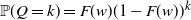 $\mathbb{P}(Q=k)=F(w)(1-F(w))^{k}$
for
$\mathbb{P}(Q=k)=F(w)(1-F(w))^{k}$
for
 $k=0,1,\ldots$
, and, in addition, Q is independent of the
$k=0,1,\ldots$
, and, in addition, Q is independent of the
 $X_{i}$
, so that
$X_{i}$
, so that
 $S_{Q}=X_{1}+\cdots+X_{Q}$
is a geometric convolution (with
$S_{Q}=X_{1}+\cdots+X_{Q}$
is a geometric convolution (with
 $S_{0}=0$
). Concerning that, [Reference Brown14, Theorem 2.1] provides a lower bound for the probability
$S_{0}=0$
). Concerning that, [Reference Brown14, Theorem 2.1] provides a lower bound for the probability
 $\mathbb{P}(S_{Q}>t)=\mathbb{P}(G_{t} > w)$
which, under our setup, yields
$\mathbb{P}(S_{Q}>t)=\mathbb{P}(G_{t} > w)$
which, under our setup, yields
 \begin{equation*} \mathbb{P}(D_{t} > w) \geq (1-F(w))\exp\bigg\{{-}\frac{F(w)}{1-F(w)}\bigg(\frac{t}{\mathbb{E}[X_{1}]}+\frac{\mathbb{E}[X_{1}^{2}]}{\mathbb{E}[X_{1}]^{2}}-1\bigg)\bigg\}.\end{equation*}
Moreover, in the special case where the distribution of
 $X_{i}$
possesses the ‘new better than used in expectation’ (NBUE) property [Reference Barlow and Proschan9, Reference Shaked and Shanthikumar33], [Reference Brown14, (3.1.10)] yields an improved lower bound for the probability
$X_{i}$
possesses the ‘new better than used in expectation’ (NBUE) property [Reference Barlow and Proschan9, Reference Shaked and Shanthikumar33], [Reference Brown14, (3.1.10)] yields an improved lower bound for the probability
 $\mathbb{P}(S_{Q}>t)=\mathbb{P}(G_{t} > w)$
which, in our case, gives
$\mathbb{P}(S_{Q}>t)=\mathbb{P}(G_{t} > w)$
which, in our case, gives
 \begin{equation} \mathbb{P}(D_{t} > w) \geq (1-F(w))\exp\bigg\{{-}\frac{t\,F(w)}{(1-F(w))\mathbb{E}[X_{1}]}\bigg\} \;=\!:\; \mathit{LB}_{_{\mathrm{Br}}}(w).\end{equation}
In what follows, we mainly focus on applications where the
 $X_{i}$
have an absolutely continuous distribution (e.g. exponential, gamma, uniform). However, it should be noted that Theorems 2 and 3 as well as Proposition 2 are valid regardless of the existence of a density for the distribution of the
$X_{i}$
have an absolutely continuous distribution (e.g. exponential, gamma, uniform). However, it should be noted that Theorems 2 and 3 as well as Proposition 2 are valid regardless of the existence of a density for the distribution of the
 $X_{i}$
.
$X_{i}$
.
Next, we consider a Poisson counting process
 $\{N_{t},t\geq0\}$
with constant intensity
$\{N_{t},t\geq0\}$
with constant intensity
 $\lambda\in(0,+\infty)$
, which is a special case of a renewal process. As is already known, in a Poisson process the interarrival times
$\lambda\in(0,+\infty)$
, which is a special case of a renewal process. As is already known, in a Poisson process the interarrival times
 $X_{1},X_{2},\ldots$
follow the exponential distribution
$X_{1},X_{2},\ldots$
follow the exponential distribution
 $\mathcal{E}(\lambda)$
with parameter
$\mathcal{E}(\lambda)$
with parameter
 $\lambda\in(0,+\infty)$
, and the kth arrival epochs
$\lambda\in(0,+\infty)$
, and the kth arrival epochs
 $S_{k}=\sum_{i=1}^{k}X_{i}$
have the Erlang (gamma) distribution with scale parameter
$S_{k}=\sum_{i=1}^{k}X_{i}$
have the Erlang (gamma) distribution with scale parameter
 $\lambda$
and shape parameter k, to be denoted by
$\lambda$
and shape parameter k, to be denoted by
 $\mathcal{G}(k,\lambda)$
.
$\mathcal{G}(k,\lambda)$
.
As a consequence of Theorem 3, we immediately derive the next result for a Poisson counting process.
Corollary 1. Let
 $D_{t}\;:\!=\;\min\{X_{1},X_{2},\ldots,X_{N_{t}+1}\}$
be the minimal spacing that starts in the time interval [0, t] in a Poisson process
$D_{t}\;:\!=\;\min\{X_{1},X_{2},\ldots,X_{N_{t}+1}\}$
be the minimal spacing that starts in the time interval [0, t] in a Poisson process
 $\{N_{t},t\geq0\}$
. Moreover, consider a Poisson RV K with parameter
$\{N_{t},t\geq0\}$
. Moreover, consider a Poisson RV K with parameter
 $\lambda t$
, independent of the
$\lambda t$
, independent of the
 $X_{i}$
. Then
$X_{i}$
. Then
 $\min\{X_{1},X_{2},\ldots,X_{K+1}\}\preceq_{\mathrm{st}}D_{t}$
.
$\min\{X_{1},X_{2},\ldots,X_{K+1}\}\preceq_{\mathrm{st}}D_{t}$
.
We are also interested in the exact distribution of the minimal spacing
 $D_{t}$
when dealing with a Poisson process. In the next proposition, an explicit formula is provided for the tail probability
$D_{t}$
when dealing with a Poisson process. In the next proposition, an explicit formula is provided for the tail probability
 $\mathbb{P}(D_{t} > w)$
. The key point for its proof lies in Theorem 2 and the loss of memory of the exponential distribution.
$\mathbb{P}(D_{t} > w)$
. The key point for its proof lies in Theorem 2 and the loss of memory of the exponential distribution.
In what follows, for any RV X and an event A, by
 $[X\mid A]$
we shall denote an RV whose distribution is the conditional distribution of X given A. We shall also use the standard notation
$[X\mid A]$
we shall denote an RV whose distribution is the conditional distribution of X given A. We shall also use the standard notation
 $\Gamma(a,z)\;:\!=\;\int_{z}^{\infty}x^{a-1}{\mathrm{e}}^{-x}\,{\mathrm{d}} x$
, with
$\Gamma(a,z)\;:\!=\;\int_{z}^{\infty}x^{a-1}{\mathrm{e}}^{-x}\,{\mathrm{d}} x$
, with
 $a>0$
and
$a>0$
and
 $z\geq0$
, for the incomplete gamma function, where
$z\geq0$
, for the incomplete gamma function, where
 $\Gamma(k)=\Gamma(k,0)=(k-1)!$
for
$\Gamma(k)=\Gamma(k,0)=(k-1)!$
for
 $k=0,1,2,\ldots$
Proposition 1. Let
 $\{N_{t},t\geq0\}$
be a Poisson process with intensity
$\{N_{t},t\geq0\}$
be a Poisson process with intensity
 $\lambda\in(0,+\infty)$
, and
$\lambda\in(0,+\infty)$
, and
 $X_{1},X_{2},\ldots$
the interarrival spacings between successive appearances of events. If
$X_{1},X_{2},\ldots$
the interarrival spacings between successive appearances of events. If
 $T=N_{t}+1$
, then the distribution of the minimal spacing
$T=N_{t}+1$
, then the distribution of the minimal spacing
 $D_{t}=\min\{X_{1},X_{2},\ldots,X_{T}\}$
that starts in the time interval [0, t] is given by
$D_{t}=\min\{X_{1},X_{2},\ldots,X_{T}\}$
that starts in the time interval [0, t] is given by
 \begin{equation*} \mathbb{P}(D_{t} > w) = \begin{cases} {\displaystyle (1-{\mathrm{e}}^{-\lambda w})\sum_{k=1}^{\lfloor{t}/{w}\rfloor}{\mathrm{e}}^{-\lambda wk} \frac{\Gamma(k,\lambda(t-kw))}{(k-1)!} + {\mathrm{e}}^{-\lambda w(\lfloor{t}/{w}\rfloor+1)},} & 0 < w < t, \\ {\mathrm{e}}^{-\lambda w}, & w\geq t, \end{cases} \end{equation*}
where
 $\lfloor{t}/{w}\rfloor$
is the integer part of
$\lfloor{t}/{w}\rfloor$
is the integer part of
 ${t}/{w}$
.
${t}/{w}$
.
Proof. Applying Theorem 2 combined with the fact that the
 $X_{i}$
are exponential distributed with parameter
$X_{i}$
are exponential distributed with parameter
 $\lambda$
(and thus
$\lambda$
(and thus
 $F(w)=1-{\mathrm{e}}^{-\lambda w}$
,
$F(w)=1-{\mathrm{e}}^{-\lambda w}$
,
 $w\geq0$
), we immediately conclude that
$w\geq0$
), we immediately conclude that
 \begin{equation} \mathbb{P}(D_{t} > w) = (1-{\mathrm{e}}^{-\lambda w})\sum_{k=1}^{\infty}{\mathrm{e}}^{-\lambda wk} \mathbb{P}(S_{k} > t \mid X_{i} > w\ \text{for all}\ i=1,\ldots,k), \quad 0 < w < t, \end{equation}
and
 $\mathbb{P}(D_{t} > w)=1-F(w)={\mathrm{e}}^{-\lambda w}$
for
$\mathbb{P}(D_{t} > w)=1-F(w)={\mathrm{e}}^{-\lambda w}$
for
 $w\geq t$
. Exploiting the loss of memory of the exponential distribution, i.e.
$w\geq t$
. Exploiting the loss of memory of the exponential distribution, i.e.
 $[X_{i}\mid X_{i}>w] =_{\mathrm{st}} X_{i}+w$
, we obtain that
$[X_{i}\mid X_{i}>w] =_{\mathrm{st}} X_{i}+w$
, we obtain that
 \begin{align} \mathbb{P}(S_{k}\geq t \mid X_{i}>w\ \text{for all}\ i=1,2,\ldots,k) & = \mathbb{P}(S_{k}\geq t-kw) \nonumber \\ & = \begin{cases} \dfrac{\Gamma(k,\lambda(t-kw))}{\Gamma(k)}, & 1\leq k\leq{t}/{w}, \\ 1, & k>{t}/{w}, \end{cases} \end{align}
since, in this case,
 $S_{k}$
follows the gamma distribution
$S_{k}$
follows the gamma distribution
 $\mathcal{G}(k,\lambda)$
. Hence, for
$\mathcal{G}(k,\lambda)$
. Hence, for
 $t>w$
, (6) in virtue of (7) yields
$t>w$
, (6) in virtue of (7) yields
 \begin{align*} \mathbb{P}(D_{t} > w) & = (1-{\mathrm{e}}^{-\lambda w})\Bigg(\sum_{k=1}^{\lfloor{t}/{w}\rfloor}{\mathrm{e}}^{-\lambda wk} \frac{\Gamma(k,\lambda(t-kw))}{\Gamma(k)} + \sum_{k=\lfloor{t}/{w}\rfloor+1}^{\infty}{\mathrm{e}}^{-\lambda wk} \times 1\Bigg) \\ & = (1-{\mathrm{e}}^{-\lambda w})\Bigg(\sum_{k=1}^{\lfloor{t}/{w}\rfloor}{\mathrm{e}}^{-\lambda wk} \frac{\Gamma(k,\lambda(t-kw))}{\Gamma(k)} + \frac{{\mathrm{e}}^{-\lambda w(\lfloor{t}/{w}\rfloor+1)}}{1-{\mathrm{e}}^{-\lambda w}}\Bigg) \\ & = (1-{\mathrm{e}}^{-\lambda w})\sum_{k=1}^{\lfloor{t}/{w}\rfloor}{\mathrm{e}}^{-\lambda wk} \frac{\Gamma(k,\lambda(t-kw))}{\Gamma(k)} + {\mathrm{e}}^{-\lambda w(\lfloor{t}/{w}\rfloor+1)}, \end{align*}
and the proof is complete.
It is well known that
 \begin{equation} \frac{\Gamma(k,\lambda(t-kw))}{\Gamma(k)} = {\mathrm{e}}^{-\lambda(t-kw)}\sum_{i=0}^{k-1}\frac{\lambda^{i}(t-kw)^{i}}{i!},\end{equation}
and therefore the tail probability of
 $D_{t}$
in Proposition 1 can be equivalently written as
$D_{t}$
in Proposition 1 can be equivalently written as
 \begin{align*} \mathbb{P}(D_{t} > w) = (1-{\mathrm{e}}^{-\lambda w}){\mathrm{e}}^{-\lambda t}\sum_{k=1}^{\lfloor{t}/{w}\rfloor}\sum_{i=0}^{k-1} \frac{\lambda^{i}(t-kw)^{i}}{i!} + {\mathrm{e}}^{-\lambda w(\lfloor{t}/{w}\rfloor+1)}\end{align*}
for
 $0 < w < t$
.
$0 < w < t$
.
Recalling (7) in the proof of Proposition 1, the equality
 \begin{equation} \mathbb{P}(S_{k}\geq t \mid X_{i}>w\ \text{for all}\ i=1,2,\ldots,k) = \mathbb{P}(S_{k}\geq t-kw)\end{equation}
enabled us to express the probability
 $\mathbb{P}(D_{t}> w)$
directly through the distribution of
$\mathbb{P}(D_{t}> w)$
directly through the distribution of
 $S_{k}$
. This relation is a consequence of the memoryless property of the exponential distribution, which implies that
$S_{k}$
. This relation is a consequence of the memoryless property of the exponential distribution, which implies that
 $[X_{i}\mid X_{i}>w]=_{\mathrm{st}}X_{i}+w$
.
$[X_{i}\mid X_{i}>w]=_{\mathrm{st}}X_{i}+w$
.
Apart from the exponential and geometric distributions, no other cases exist where (9) is valid. However, there are classes of distributions where we may get inequality instead of equality in (9). In this respect, we note the definition of the well-known IFR and DFR classes of distributions (cf. [Reference Barlow and Proschan9, Reference Shaked and Shanthikumar33]).
Definition 2. An RV X (or its distribution) with CDF F is said to be IFR (increasing failure rate) or DFR (decreasing failure rate) when the function
 $1-F$
is log-concave or log-convex, respectively.
$1-F$
is log-concave or log-convex, respectively.
Exploiting [Reference Shaked and Shanthikumar33, Theorem 1.A.30(a)], we get the following stochastic relations for non-negative IFR and DFR RVs by means of the usual stochastic order. Specifically, for a non-negative IFR (DFR) RV X,
 \begin{equation} [X \mid X>w] \preceq_{\mathrm{st}} (\succeq_{\mathrm{st}})\,X+w.\end{equation}
We note that the exponential distribution is both IFR and DFR.
Considering all the above, we derive the following general result for the survival function of the minimal spacing
 $D_{t}$
in a renewal process with IFR or DFR interarrival times.
$D_{t}$
in a renewal process with IFR or DFR interarrival times.
Proposition 2. If the interarrival spacings
 $X_{1},X_{2},\ldots$
between successive appearances of events in a renewal process are IFR (DFR), then
$X_{1},X_{2},\ldots$
between successive appearances of events in a renewal process are IFR (DFR), then
 \begin{equation*} \mathbb{P}(D_{t} > w) \leq (\geq)\,F(w)\sum_{k=1}^{\lfloor{t}/{w}\rfloor}(1-F(w))^{k} \mathbb{P}(S_{k} > t-kw) + (1-F(w))^{\lfloor{t}/{w}\rfloor+1}, \quad 0 < w < t, \end{equation*}
where
 $S_{k}=\sum_{i=1}^{k}X_{i}$
. Equality holds when the
$S_{k}=\sum_{i=1}^{k}X_{i}$
. Equality holds when the
 $X_{i}$
are exponentially distributed.
$X_{i}$
are exponentially distributed.
Proof. Under the assumption that the
 $X_{i}$
are IFR (DFR), property (10) and the fact that the usual stochastic order is closed under convolutions together yield
$X_{i}$
are IFR (DFR), property (10) and the fact that the usual stochastic order is closed under convolutions together yield
 \begin{align*} \mathbb{P}(S_{k}\geq t \mid X_{i}>w\ \text{for all}\ i=1,2,\ldots,k) \leq (\geq)\,\mathbb{P}(S_{k}\geq t-kw) \end{align*}
and the result follows from Theorem 2, similarly to the proof of Proposition 1.
It can be easily verified that the lower bound of Proposition 2 is always better (larger) than that of Theorem 3 (since
 $\mathbb{P}(S_{k}>t)\leq\mathbb{P}(S_{k}>t-kw)$
), a fact that is intuitively expected since the former bound refers to a smaller class of distributions that possess the DFR property, whereas the latter one is more general.
$\mathbb{P}(S_{k}>t)\leq\mathbb{P}(S_{k}>t-kw)$
), a fact that is intuitively expected since the former bound refers to a smaller class of distributions that possess the DFR property, whereas the latter one is more general.
Example 1. As an example, we assume that the spacings
 $X_{i}$
follow the Gamma distribution
$X_{i}$
follow the Gamma distribution
 $\mathcal{G}(a,\lambda)$
with density
$\mathcal{G}(a,\lambda)$
with density
 $f(x)=({\lambda^{a}}/{\Gamma(a)})x^{a-1}{\mathrm{e}}^{^{-\lambda x}}\boldsymbol{1}[x>0]$
, which is IFR when
$f(x)=({\lambda^{a}}/{\Gamma(a)})x^{a-1}{\mathrm{e}}^{^{-\lambda x}}\boldsymbol{1}[x>0]$
, which is IFR when
 $a\geq1$
and DFR when
$a\geq1$
and DFR when
 $0 < a\leq1$
[Reference Marshall and Olkin27]. Since, in this case,
$0 < a\leq1$
[Reference Marshall and Olkin27]. Since, in this case,
 $S_{k}=\sum_{i=1}^{k}X_{i}$
has the gamma distribution
$S_{k}=\sum_{i=1}^{k}X_{i}$
has the gamma distribution
 $\mathcal{G}(ka,\lambda)$
, Proposition 2 directly yields, for
$\mathcal{G}(ka,\lambda)$
, Proposition 2 directly yields, for
 $a>1$
(
$a>1$
(
 $0 < a < 1$
) and
$0 < a < 1$
) and
 $0 < w < t$
,
$0 < w < t$
,
 \begin{align} \mathbb{P}(D_{t} > w) & \leq (\geq)\,\bigg(1-\frac{\Gamma(a,\lambda w)}{\Gamma(a)}\bigg) \sum_{k=1}^{\lfloor{t}/{w}\rfloor}\bigg(\frac{\Gamma(a,\lambda w)}{\Gamma(a)}\bigg)^{k} \frac{\Gamma(ka,\lambda(t-kw))}{\Gamma(ka)} \nonumber \\ & \qquad\quad + \bigg(\frac{\Gamma(a,\lambda w)}{\Gamma(a)}\bigg)^{(\lfloor{t}/{w}\rfloor+1)}, \end{align}
whereas for
 $w\geq t$
,
$w\geq t$
,
 $\mathbb{P}(D_{t} > w) = \Gamma(a,\lambda w)/\Gamma(a)$
for all
$\mathbb{P}(D_{t} > w) = \Gamma(a,\lambda w)/\Gamma(a)$
for all
 $a>0$
.
$a>0$
.
Next, we return to the case of a Poisson process. Aside from the explicit formula of Proposition 1 for the exact distribution of
 $D_{t}$
, it would be quite useful to have at hand easily computable closed-form upper and lower bounds for the tail probability
$D_{t}$
, it would be quite useful to have at hand easily computable closed-form upper and lower bounds for the tail probability
 $\mathbb{P}(D_{t} > w)$
that can also lead to asymptotic results. We offer the following proposition.
$\mathbb{P}(D_{t} > w)$
that can also lead to asymptotic results. We offer the following proposition.
Proposition 3. Consider a Poisson process
 $\{N_{t},t\geq0\}$
with intensity
$\{N_{t},t\geq0\}$
with intensity
 $\lambda\in(0,+\infty)$
and interarrival spacings
$\lambda\in(0,+\infty)$
and interarrival spacings
 $X_{1},X_{2},\ldots$
between successive appearances of events. If
$X_{1},X_{2},\ldots$
between successive appearances of events. If
 $T=N_{t}+1$
and
$T=N_{t}+1$
and
 $D_{t}=\min\{X_{1},X_{2},\ldots,X_{T}\}$
, then for
$D_{t}=\min\{X_{1},X_{2},\ldots,X_{T}\}$
, then for
 $t>w>0$
and
$t>w>0$
and
 $\lambda t>1$
,
$\lambda t>1$
,
 $L(\lambda,t,w)\mathbb{\leq P}(D_{t} > w)\leq U(\lambda,t,w)$
, where
$L(\lambda,t,w)\mathbb{\leq P}(D_{t} > w)\leq U(\lambda,t,w)$
, where
 \begin{align*} L(\lambda,t,w) & \;:\!=\; \exp\{-\lambda w-\lambda t(1-{\mathrm{e}}^{-\lambda w})\}, \\ U(\lambda,t,w) & \;:\!=\; \exp\bigg\{{-}\lambda w - \lambda\bigg(t-w\bigg\lfloor\frac{1}{w}\sqrt{\frac{t}{\lambda}}\bigg\rfloor\bigg)(1-{\mathrm{e}}^{-\lambda w})\bigg\} + \exp\bigg\{{-}\lambda w\bigg(\bigg\lfloor\frac{1}{w}\sqrt{\frac{t}{\lambda}}\bigg\rfloor+1\bigg)\bigg\}. \end{align*}
Proof. Applying Proposition 1 for
 $w<t$
, we get
$w<t$
, we get
 \begin{equation} \mathbb{P}(D_{t} > w) = c(\lambda,t,w) + {\mathrm{e}}^{-\lambda w(\lfloor{t}/{w}\rfloor+1)}, \end{equation}
where, for convenience, we set
 \begin{align*} c(\lambda,t,w) \;:\!=\; (1-{\mathrm{e}}^{-\lambda w})\sum_{k=1}^{\lfloor{t}/{w}\rfloor}{\mathrm{e}}^{-\lambda wk} \frac{\Gamma(k,\lambda(t-kw))}{\Gamma(k)}. \end{align*}
The summand
 $c(\lambda,t,w)$
will lead us to the desired upper bound, and hence we will treat it separately. So, recalling that
$c(\lambda,t,w)$
will lead us to the desired upper bound, and hence we will treat it separately. So, recalling that
 $\Gamma(k,\lambda(t-kw))/\Gamma(k)=\mathbb{P}(S_{k}\geq t-kw)\leq1$
, and taking into consideration that
$\Gamma(k,\lambda(t-kw))/\Gamma(k)=\mathbb{P}(S_{k}\geq t-kw)\leq1$
, and taking into consideration that
 $\Gamma(k,\lambda(t-kw))\leq\Gamma(k,\lambda(t-bw))$
when
$\Gamma(k,\lambda(t-kw))\leq\Gamma(k,\lambda(t-bw))$
when
 $k\leq b\;:\!=\;\lfloor({1}/{w})\sqrt{{t}/{\lambda}}\rfloor$
, we obtain
$k\leq b\;:\!=\;\lfloor({1}/{w})\sqrt{{t}/{\lambda}}\rfloor$
, we obtain
 \begin{align} c(\lambda,t,w) & = (1-{\mathrm{e}}^{-\lambda w})\Bigg\{\sum_{k=1}^{b}{\mathrm{e}}^{-\lambda wk}\frac{\Gamma(k,\lambda(t-kw))}{\Gamma(k)} + \sum_{k=b+1}^{\lfloor{t}/{w}\rfloor}{\mathrm{e}}^{-\lambda wk}\frac{\Gamma(k,\lambda(t-kw))}{\Gamma(k)}\Bigg\} \nonumber \\ & \leq (1-{\mathrm{e}}^{-\lambda w})\Bigg\{\sum_{k=1}^{\infty}{\mathrm{e}}^{-\lambda wk}\frac{\Gamma(k,\lambda(t-bw))}{\Gamma(k)} + \sum_{k=b+1}^{\lfloor{t}/{w}\rfloor}{\mathrm{e}}^{-\lambda wk}\Bigg\} . \end{align}
As will become apparent, the splitting of the summation at b was chosen so that we get a simple-in-form upper bound that is asymptotically sharp (cf. the proof of Theorem 4). The first summation in (13) is now equal to
 \begin{align*} \sum_{k=1}^{\infty}\frac{{\mathrm{e}}^{-\lambda wk}}{\Gamma(k)}\int_{\lambda(t-bw)}^{\infty}s^{k-1}{\mathrm{e}}^{-s}\,{\mathrm{d}} s & = \int_{\lambda(t-bw)}^{\infty}{\mathrm{e}}^{-s}\Bigg(\sum_{k=1}^{\infty}\frac{{\mathrm{e}}^{-\lambda wk}}{\Gamma(k)}s^{k-1}\Bigg)\,{\mathrm{d}} s \\ & = \frac{{\mathrm{e}}^{-\lambda w}\exp\{-\lambda(t-bw)(1-{\mathrm{e}}^{-\lambda w})\}}{1-{\mathrm{e}}^{-\lambda w}}, \end{align*}
where the interchange of summation and integration is allowed by Tonelli’s theorem. Therefore,
 \begin{align*} c(\lambda,t,w) & \leq (1-{\mathrm{e}}^{-\lambda w})\Bigg\{\frac{{\mathrm{e}}^{-\lambda w}\exp\{-\lambda(t-bw)(1-{\mathrm{e}}^{-\lambda w})\}}{1-{\mathrm{e}}^{-\lambda w}} + \sum_{k=b+1}^{\lfloor{t}/{w}\rfloor}{\mathrm{e}}^{-\lambda wk}\Bigg\} \nonumber \\ & = {\mathrm{e}}^{-\lambda w}\exp\{-\lambda(t-bw)(1-{\mathrm{e}}^{-\lambda w})\} + {\mathrm{e}}^{-\lambda w(b+1)} - {\mathrm{e}}^{-\lambda w(\lfloor{t}/{w}\rfloor+1)}. \end{align*}
Combining this with (12), we finally obtain the upper bound
 \begin{align*} \mathbb{P}(D_{t} > w) \leq {\mathrm{e}}^{-\lambda w}\exp\{-\lambda(t-bw)(1-{\mathrm{e}}^{-\lambda w})\} + {\mathrm{e}}^{-\lambda w(b+1)} \;=\!:\; U(\lambda,t,w). \end{align*}
The lower bound
 $L(\lambda,t,w)$
will be derived by Corollary 1. In particular, by a straightforward application of this corollary we deduce that
$L(\lambda,t,w)$
will be derived by Corollary 1. In particular, by a straightforward application of this corollary we deduce that
 $\mathbb{P}(G_{t} > w) \leq \mathbb{P}(D_{t} > w)$
,
$\mathbb{P}(G_{t} > w) \leq \mathbb{P}(D_{t} > w)$
,
 $w\in(0,\infty)$
. Invoking the second equality of (4) in the proof of Theorem 3, and recalling that
$w\in(0,\infty)$
. Invoking the second equality of (4) in the proof of Theorem 3, and recalling that
 $K_{t}$
has the Poisson distribution with parameter
$K_{t}$
has the Poisson distribution with parameter
 $\lambda t$
since
$\lambda t$
since
 $K_{t}=_{\mathrm{st}}N_{t}$
, we get
$K_{t}=_{\mathrm{st}}N_{t}$
, we get
 \begin{align*} \mathbb{P}(G_{t} > w) & = \sum_{k=0}^{\infty}\mathbb{P}(\!\min\{X_{1},X_{2},\ldots,X_{k+1}\} > w)P(K_{t}=k) \\ & = \sum_{k=0}^{\infty}{\mathrm{e}}^{-\lambda w(k+1)}{\mathrm{e}}^{-\lambda t}\frac{(\lambda t)^{k}}{k!} = \exp\{-\lambda w-\lambda t(1-{\mathrm{e}}^{-\lambda w})\}, \end{align*}
which is exactly the lower bound
 $L(\lambda,t,w)$
.
$L(\lambda,t,w)$
.
Although an exact formula for the distribution of
 $D_{t}$
in a Poisson process has been obtained in Proposition 1, it is also of theoretical as well as practical interest to investigate its asymptotic behaviour. In particular, it is shown below that, under general conditions, the minimum spacing
$D_{t}$
in a Poisson process has been obtained in Proposition 1, it is also of theoretical as well as practical interest to investigate its asymptotic behaviour. In particular, it is shown below that, under general conditions, the minimum spacing
 $D_{t}$
satisfies an asymptotic result.
$D_{t}$
satisfies an asymptotic result.
Theorem 4. Let
 $\{N_{t},t\geq0\}$
be a Poisson process with intensity
$\{N_{t},t\geq0\}$
be a Poisson process with intensity
 $\lambda\in(0,+\infty)$
and
$\lambda\in(0,+\infty)$
and
 $X_{1},X_{2},\ldots$
the interarrival times between successive appearances of events. Set
$X_{1},X_{2},\ldots$
the interarrival times between successive appearances of events. Set
 $T=N_{t}+1$
. Then, as
$T=N_{t}+1$
. Then, as
 $\lambda t\to\infty$
,
$\lambda t\to\infty$
,
 $\lim_{\lambda t\to\infty}\mathbb{P}(\lambda^{2}tD_{t}>x) = {\mathrm{e}}^{-x}$
,
$\lim_{\lambda t\to\infty}\mathbb{P}(\lambda^{2}tD_{t}>x) = {\mathrm{e}}^{-x}$
,
 $x>0$
; in other words,
$x>0$
; in other words,
 $\lambda^{2}tD_{t}$
converges in distribution to
$\lambda^{2}tD_{t}$
converges in distribution to
 $\mathcal{E}(1)$
as
$\mathcal{E}(1)$
as
 $\lambda t\to\infty$
.
$\lambda t\to\infty$
.
Proof. For
 $w={x}/(\lambda^{2}t)>0$
, Proposition 3 yields
$w={x}/(\lambda^{2}t)>0$
, Proposition 3 yields
 \begin{equation} L\bigg(\lambda,t,\frac{x}{\lambda^{2}t}\bigg) \leq \mathbb{P}(\lambda^{2}tD_{t}>x) \leq U\bigg(\lambda,t,\frac{x}{\lambda^{2}t}\bigg). \end{equation}
It can be easily verified that, for
 $x>0$
,
$x>0$
,
 \begin{equation} \lim_{\lambda t\to\infty}L\bigg(\lambda,t,\frac{x}{\lambda^{2}t}\bigg) = \lim_{\lambda t\to\infty}\{{\mathrm{e}}^{-{x}/({\lambda t})}\exp\{-\lambda t\,(1-e^{-{x}/({\lambda t})})\}\} = {\mathrm{e}}^{-x}. \end{equation}
Moreover, the following limit relations also hold:
 \begin{align*} \lim_{\lambda t\rightarrow\infty}\exp\bigg\{{-}\frac{x}{\lambda t} \bigg(\bigg\lfloor\frac{(\lambda t)^{3/2}}{x}\bigg\rfloor + 1\bigg)\bigg\} & = 0, \\ \lim_{\lambda t\rightarrow\infty}\bigg({\mathrm{e}}^{-{x}/({\lambda t})} \exp\bigg\{{-}\bigg(\lambda t-\bigg\lfloor\frac{(\lambda t)^{3/2}}{x}\bigg\rfloor \frac{x}{\lambda t}\bigg)(1-e^{-{x}/({\lambda t})})\bigg\}\bigg) & = {\mathrm{e}}^{-x}. \end{align*}
Consequently,
 \begin{equation} \lim_{\lambda t\to\infty}U\bigg(\lambda,t,\frac{x}{\lambda^{2}t}\bigg) = {\mathrm{e}}^{-x}. \end{equation}
Thus, combining (14) with (15) and (16), we finally obtain the desired approximation result.
The previous asymptotic outcome implies that, for large
 $\lambda t$
, it is approximately
$\lambda t$
, it is approximately
 $\mathbb{P}(D_{t} > w )\simeq {\mathrm{e}}^{-w\lambda^{2}t}$
.
$\mathbb{P}(D_{t} > w )\simeq {\mathrm{e}}^{-w\lambda^{2}t}$
.
Note that in the aforementioned results we were mainly concerned with the minimum spacing in a Poisson process, due to the theoretical importance, applicability, and nice properties of this process. However, it is worth stressing that Theorem 2 is valid for every renewal process. Hence, in order to illustrate its wider applicability, we now present two additional results concerning the minimum spacing for specific non-exponential distributions of the interarrival times.
Initially, we shall extract an explicit formula for the survival function of
 $D_{t}$
when the interarrival times of the renewal process follow the Erlang distribution
$D_{t}$
when the interarrival times of the renewal process follow the Erlang distribution
 $\mathcal{G}(2,\lambda)$
.
$\mathcal{G}(2,\lambda)$
.
Proposition 4. If the CDF of the interarrival times
 $X_{1},X_{2},\ldots$
of a renewal process is given by
$X_{1},X_{2},\ldots$
of a renewal process is given by
 $F(x) = 1 - {\mathrm{e}}^{-\lambda x}(1+\lambda x)$
,
$F(x) = 1 - {\mathrm{e}}^{-\lambda x}(1+\lambda x)$
,
 $x\geq0$
, then, for
$x\geq0$
, then, for
 $0 < w < t$
,
$0 < w < t$
,
 \begin{align*} \mathbb{P}(D_{t} > w) & = (1-{\mathrm{e}}^{-\lambda w}(1+\lambda w)){\mathrm{e}}^{-\lambda t}\sum_{k=1}^{\lfloor{t}/{w}\rfloor}\sum_{\nu=0}^{k} \binom{k}{\nu}(\lambda w)^{\nu}\sum_{i=0}^{2k-\nu-1}\frac{\lambda^{i}(t-kw)^{i}}{i!} \\ & \quad + ({\mathrm{e}}^{-\lambda w}(1+\lambda w))^{\lfloor{t}/{w}\rfloor+1} \end{align*}
and
 $\mathbb{P}(D_{t} > w) = {\mathrm{e}}^{-\lambda w}(1+\lambda w)$
for
$\mathbb{P}(D_{t} > w) = {\mathrm{e}}^{-\lambda w}(1+\lambda w)$
for
 $w\geq t$
.
$w\geq t$
.
Proof. In this case, the conditional distribution of
 $[X_{i}-w \mid X_{i}>w]$
is a mixture of an exponential
$[X_{i}-w \mid X_{i}>w]$
is a mixture of an exponential
 $\mathcal{E}(\lambda)$
and an Erlang
$\mathcal{E}(\lambda)$
and an Erlang
 $\mathcal{G}(2,\lambda)$
distribution. Indeed, for
$\mathcal{G}(2,\lambda)$
distribution. Indeed, for
 $t>0$
and
$t>0$
and
 $w>0$
,
$w>0$
,
 \begin{align*} \mathbb{P}(X_{i}-w>t \mid X_{i}>w) = \frac{\mathbb{P}(X_{i}>t+w)}{\mathbb{P}(X_{i}>w)} & = \frac{{\mathrm{e}}^{-\lambda(t+w)}(1+\lambda(t+w))}{{\mathrm{e}}^{-\lambda w}(1+\lambda w)} \\ & = \frac{{\mathrm{e}}^{-\lambda t}(1+\lambda(t+w))}{(1+\lambda w)} \\ & = p{\mathrm{e}}^{-\lambda t} + (1-p){\mathrm{e}}^{-\lambda t}(1+\lambda t), \end{align*}
where
 $p={\lambda w}/({1+\lambda w})\in(0,1)$
. Therefore,
$p={\lambda w}/({1+\lambda w})\in(0,1)$
. Therefore,
 $[X_{i}-w \mid X_{i}>w] =_{\mathrm{st}} I_{i}Z_{i}+(1-I_{i})R_{i}$
, where the RVs
$[X_{i}-w \mid X_{i}>w] =_{\mathrm{st}} I_{i}Z_{i}+(1-I_{i})R_{i}$
, where the RVs
 $I_{i}$
,
$I_{i}$
,
 $Z_{i}$
, and
$Z_{i}$
, and
 $R_{i}$
are all considered independent following a Bernoulli(p), an exponential
$R_{i}$
are all considered independent following a Bernoulli(p), an exponential
 $\mathcal{E}(\lambda)$
, and an Erlang
$\mathcal{E}(\lambda)$
, and an Erlang
 $\mathcal{G}(2,\lambda)$
distribution, respectively. Then, it follows that
$\mathcal{G}(2,\lambda)$
distribution, respectively. Then, it follows that
 \begin{align*} & \mathbb{P}(S_{k}>t \mid X_{i}>w, i=1,\ldots,k) \\ & \qquad = \mathbb{P}\Bigg(\sum_{i=1}^{k}(I_{i}Z_{i}+(1-I_{i})R_{i})>t-kw\Bigg) \\ & \qquad = \sum_{\nu=0}^{k}\mathbb{P}\Bigg(\sum_{i=1}^{k}(I_{i}Z_{i}+(1-I_{i})R_{i}) > t-kw \mid \sum_{i=1}^{k}I_{i}=\nu\Bigg)\mathbb{P}\Bigg(\sum_{i=1}^{k}I_{i}=\nu\Bigg). \end{align*}
We observe that the conditional distribution of the RV
 $\sum_{i=1}^{k}(I_{i}Z_{i}+(1-I_{i})R_{i})$
given that
$\sum_{i=1}^{k}(I_{i}Z_{i}+(1-I_{i})R_{i})$
given that
 $\sum_{i=1}^{k}I_{i}=\nu$
coincides with the distribution of
$\sum_{i=1}^{k}I_{i}=\nu$
coincides with the distribution of
 $\sum_{i=1}^{\nu}Z_{i}+\sum_{i=1}^{k-\nu}R_{i}$
, which, as a convolution of exponential and Erlang distributions, also follows the Erlang distribution with scale parameter
$\sum_{i=1}^{\nu}Z_{i}+\sum_{i=1}^{k-\nu}R_{i}$
, which, as a convolution of exponential and Erlang distributions, also follows the Erlang distribution with scale parameter
 $\lambda$
and shape parameter
$\lambda$
and shape parameter
 $\nu+2(k-\nu)=2k-\nu$
. Hence,
$\nu+2(k-\nu)=2k-\nu$
. Hence,
 \begin{align*} \mathbb{P}(S_{k}>t \mid X_{i}>w, i=1,\ldots,k) & =\sum_{\nu=0}^{k}\mathbb{P}\Bigg(\sum_{i=1}^{\nu}Z_{i}+\sum_{i=1}^{k-\nu}R_{i}>t-kw\Bigg)\binom{k}{\nu} p^{\nu}(1-p)^{k-\nu} \\ & = \sum_{\nu=0}^{k}\binom{k}{\nu}(\lambda w)^{\nu} \frac{\Gamma(2k-\nu,\lambda(t-kw))}{\Gamma(2k-\nu)(1+\lambda w)^{k}} \end{align*}
and a direct application of Theorem 2 yields, for
 $0 < w < t$
,
$0 < w < t$
,
 \begin{align*} \mathbb{P}(D_{t} > w) & = F(w)\sum_{k=1}^{\lfloor{t}/{w}\rfloor}(1-F(w))^{k}\mathbb{P}(S_{k}>t \mid X_{i}>w, i=1,\ldots,k) + (1-F(w))^{\lfloor{t}/{w}\rfloor+1} \\ & = (1-{\mathrm{e}}^{-\lambda w}(1+\lambda w))\sum_{k=1}^{\lfloor{t}/{w}\rfloor}{\mathrm{e}}^{-k\lambda w}\sum_{\nu=0}^{k} \binom{k}{\nu}(\lambda w)^{\nu}\frac{\Gamma(2k-\nu,\lambda(t-kw))}{\Gamma(2k-\nu)} \\ & \quad + ({\mathrm{e}}^{-\lambda w}(1+\lambda w))^{\lfloor{t}/{w}\rfloor+1}, \end{align*}
which, also taking (8) into account, finally completes the proof.
Before closing this section, we present an additional application of Theorem 2, this time assuming that the spacings
 $X_{1},X_{2},\ldots$
follow the uniform distribution in (0,1), to be denoted by
$X_{1},X_{2},\ldots$
follow the uniform distribution in (0,1), to be denoted by
 $\mathcal{U}(0,1)$
. In addition, we shall exploit the fact that the convolution of uniform distributions converges quickly to a normal distribution by the central limit theorem (CLT), allowing us to employ a normal approximation for the summands when t is relatively large (e.g. greater than 3 will suffice; see Figure 3). In what follows,
$\mathcal{U}(0,1)$
. In addition, we shall exploit the fact that the convolution of uniform distributions converges quickly to a normal distribution by the central limit theorem (CLT), allowing us to employ a normal approximation for the summands when t is relatively large (e.g. greater than 3 will suffice; see Figure 3). In what follows,
 $\mathrm{sgn}(x)$
denotes the sign of x.
$\mathrm{sgn}(x)$
denotes the sign of x.
Proposition 5. Suppose that the interarrival times
 $X_{1},X_{2},\ldots$
of a renewal process follow the uniform distribution
$X_{1},X_{2},\ldots$
of a renewal process follow the uniform distribution
 $\mathcal{U}(0,1)$
. Then:
$\mathcal{U}(0,1)$
. Then:
-
(i) For
 $0 < w < 1$
and
$w<t$
, the exact distribution of
$D_{t}$
is given by whereas for
\begin{align*} \mathbb{P}(D_{t} > w) & = w\sum_{k=\lfloor t\rfloor+1}^{\lfloor{t}/{w}\rfloor}\sum_{j=0}^{k}\frac{(-1)^{^{j+1}}}{2k!}\binom{k}{j} (t-kw-(1-w)j)^{k}\mathrm{sgn}\bigg(\frac{t-kw}{1-w}-j\bigg) \\ & \quad + \frac{1}{2}[(1-w)^{\lfloor t\rfloor+1} + (1-w)^{\lfloor{t}/{w}\rfloor+1}], \end{align*}
$0\leq t\leq w < 1$
,
$\mathbb{P}(D_{t} > w)=1-w$
.
$0 < w < 1$
and
$w<t$
, the exact distribution of
$D_{t}$
is given by whereas for
\begin{align*} \mathbb{P}(D_{t} > w) & = w\sum_{k=\lfloor t\rfloor+1}^{\lfloor{t}/{w}\rfloor}\sum_{j=0}^{k}\frac{(-1)^{^{j+1}}}{2k!}\binom{k}{j} (t-kw-(1-w)j)^{k}\mathrm{sgn}\bigg(\frac{t-kw}{1-w}-j\bigg) \\ & \quad + \frac{1}{2}[(1-w)^{\lfloor t\rfloor+1} + (1-w)^{\lfloor{t}/{w}\rfloor+1}], \end{align*}
$0\leq t\leq w < 1$
,
$\mathbb{P}(D_{t} > w)=1-w$
.
-
(ii) For
$0 < w < 1$
,
$w<t$
, and relatively large t, the distribution of
$D_t$
is approximately Moreover, for
\begin{align*} \mathbb{P}(D_{t} > w) \simeq A(w) \;:\!=\; w\sum_{k=\lfloor t\rfloor+1}^{\lfloor{t}/{w}\rfloor}(1-w)^{k} \Phi\bigg(\frac{(1+w)k-2t}{(1-w)\sqrt{{k}/{3}}\,}\bigg) + (1-w)^{\lfloor{t}/{w}\rfloor+1}. \end{align*}
$w\in(0,1)$
, as
\begin{align*} |\mathbb{P}(D_{t} > w)-A(w)| \leq \delta\frac{(1-w)^{\lfloor t\rfloor+1}}{\lfloor t\rfloor+1} \to 0 \end{align*}
$t\to\infty$
, where
$\delta$
is a constant less than
$0.6$
.


Proof.
-
(i) Obviously,
$F(w)=w$
,
$w\in(0,1)$
, and hence Theorem 2 yields, for
$w\in(0,1)$
, (17)and
\begin{equation} \mathbb{P}(D_{t} > w) = w\sum_{k=1}^{\infty}(1-w)^{k} \mathbb{P}(S_{k}>t \mid X_{i}>w\ \text{for all}\ i=1,\ldots,k), \quad w < t, \end{equation}
$\mathbb{P}(D_{t} > w)=1-F(w)=1-w$
for
$w\geq t$
. It can be easily verified that
$[X_{i} \mid X_{i}>w] =_{\mathrm{st}} X_{i}^{w}$
, where
$X_{i}^{w}$
follows the uniform distribution
$\mathcal{U}(w,1)$
,
$i=1,2,\ldots$
Therefore, where
\begin{align*} \mathbb{P}(S_{k}>t \mid X_{i}>w\ \text{for all}\ i=1,\ldots,k) = \mathbb{P}\big(S_{k}^{w}>t\big), \end{align*}
$S_{k}^{w}=\sum_{i=1}^{k}X_{i}^{w}$
,
$k=1,2,\ldots$
, which, combined with (17), gives, for
$w\in(0,1)$
, (18)It can be checked that
\begin{equation} \mathbb{P}(D_{t} > w) = w\sum_{k=1}^{\infty}(1-w)^{k}\mathbb{P}\big(S_{k}^{w} > t\big), \quad w < t. \end{equation}
$S_{k}^{w} =_{\mathrm{st}} (1-w)\sum_{i=1}^{k}U_{i}+kw$
, where
$U_{1},U_{2},\ldots$
is a sequence of i.i.d. uniform
$\mathcal{U}(0,1)$
RVs and, using the exact formula for the CDF of the sum
$\sum_{i=1}^{k}U_{i}$
[Reference Cramér15, Reference Mitra28], Thus, by substitution in (18), we obtain, for
\begin{align*} \mathbb{P}\big(S_{k}^{w} > t\big) & = \mathbb{P}\Bigg(\sum_{i=1}^{k}U_{i} > \frac{t-kw}{1-w}\Bigg) \\ & = \begin{cases} 0, & 1\leq k\leq t, \\ \dfrac{1}{2} - \displaystyle\sum_{j=0}^{k}\dfrac{(-1)^{^{j}}}{2k!}\displaystyle\binom{k}{j} \bigg(\dfrac{t-kw}{1-w}-j\bigg)^{k}\mathrm{sgn}\bigg(\frac{t-kw}{1-w}-j\bigg), & t < k\leq{t}/{w}, \\ 1, & k > {t}/{w}. \end{cases} \end{align*}
$w\in(0,1)$
and
$w<t$
,
\begin{align*} \mathbb{P}(D_{t} > w) & = w\sum_{k=\lfloor t \rfloor+1}^{\lfloor{t}/{w}\rfloor}(1-w)^{k} \Bigg[\frac{1}{2}-\sum_{j=0}^{k}\frac{(-1)^{^{j}}}{2k!}\binom{k}{j}\bigg(\frac{t-kw}{1-w}-j\bigg)^{k} \mathrm{sgn}\bigg(\frac{t-kw}{1-w}-j\bigg)\Bigg] \\ & \quad + w\sum_{k=\lfloor{t}/{w}\rfloor+1}^{\infty}(1-w)^{k} \\ & = w\sum_{k=\lfloor t\rfloor+1}^{\lfloor{t}/{w}\rfloor}(1-w)^{k} \Bigg[\frac{1}{2}-\sum_{j=0}^{k}\frac{(-1)^{^{j}}}{2k!}\binom{k}{j}\bigg(\frac{t-kw}{1-w}-j\bigg)^{k} \mathrm{sgn}\bigg(\frac{t-kw}{1-w}-j\bigg)\Bigg] \\ & \quad + (1-w)^{\lfloor{t}/{w}\rfloor+1} \\ & = \frac{1}{2}\big[(1-w)^{\lfloor t\rfloor+1}+(1-w)^{\lfloor{t}/{w}\rfloor+1}\big] \\ & \quad + w\sum_{k=\lfloor t\rfloor+1}^{\lfloor{t}/{w}\rfloor}\sum_{j=0}^{k}\frac{(-1)^{^{j+1}}}{2k!}\binom{k}{j} (t-kw-(1-w)j)^{k}\mathrm{sgn}\bigg(\frac{t-kw}{1-w}-j\bigg). \end{align*}
-
(ii) Applying the CLT on the sequence of the i.i.d. RVs
$X_{1}^{w},X_{2}^{w},\ldots$
for
$k\in\{\lfloor t \rfloor+1,\ldots,\lfloor{t}/{w}\rfloor\}$
and large values of t, we deduce that, approximately, which, together with (18) and the fact that
\begin{align*} \mathbb{P}\big(S_{k}^{w}>t\big) = \mathbb{P}\Bigg(\frac{\sum_{i=1}^{k}U_{i}-k/2}{\sqrt{{k}/{12}}} > \frac{({t-kw})/({1-w})-{k}/{2}}{\sqrt{{k}/{12}}}\Bigg) \simeq \Phi\bigg(\frac{(1+w)k-2t}{(1-w)\sqrt{{k}/{3}}}\bigg), \end{align*}
$\mathbb{P}(S_{k}^{w}>t)=0$
for
$k\in\{1,\ldots,\lfloor t \rfloor\}$
and
$\mathbb{P}(S_{k}^{w}>t)=1$
when
$k\in\{\lfloor{t}/{w}\rfloor+1,\ldots\}$
, yield the approximation formula of interest. Note finally that as
\begin{align*} |\mathbb{P}(D_{t} > w)-A(w)| & \leq w\sum_{k=\lfloor t\rfloor+1}^{\lfloor{t}/{w}\rfloor}(1-w)^{k} \bigg|\mathbb{P}\big(S_{k}^{w}>t\big)-\Phi\bigg(\frac{(1+w)k-2t}{(1-w)\sqrt{{k}/{3}}}\bigg)\bigg| \\ & \leq \delta w\sum_{k=\lfloor t\rfloor+1}^{\lfloor{t}/{w}\rfloor}\frac{(1-w)^{k}}{k} \leq \delta\frac{(1-w)^{\lfloor t\rfloor+1}}{\lfloor t\rfloor+1} \to 0 \end{align*}
$t\to\infty$
, where the second inequality follows from the sharp upper bound of the normal approximation error for uniformly distributed summands obtained in [Reference Uspensky37, p. 305] (see also [Reference Seoh32]), and
$\delta$
is a constant less than
$0.6$
.


4. Numerical examples
Next, we present several numerical comparisons among the exact distribution of
 $D_{t}$
, the upper/lower bounds, and the approximate formulae presented in Section 3. We begin by assuming that the events appear according to a homogeneous Poisson process with constant intensity
$D_{t}$
, the upper/lower bounds, and the approximate formulae presented in Section 3. We begin by assuming that the events appear according to a homogeneous Poisson process with constant intensity
 $\lambda$
, i.e. the spacings are exponentially distributed. The exact tail distribution of the minimal spacing
$\lambda$
, i.e. the spacings are exponentially distributed. The exact tail distribution of the minimal spacing
 $D_{t}$
that starts in a time interval [0, t] is given by Proposition 1 and is depicted for explicit values of the parameters in Figures 1 and 2, along with the upper and lower bounds
$D_{t}$
that starts in a time interval [0, t] is given by Proposition 1 and is depicted for explicit values of the parameters in Figures 1 and 2, along with the upper and lower bounds
 $U(\lambda,t,w)$
and
$U(\lambda,t,w)$
and
 $L(\lambda,t,w)$
provided by Proposition 3 and the lower bound
$L(\lambda,t,w)$
provided by Proposition 3 and the lower bound
 $\mathit{LB}_{\mathrm{Br}}(w)$
of [Reference Brown14] for NBUE interarrival times given by (5) – the exponential distribution has the NBUE property. Note that the upper bound
$\mathit{LB}_{\mathrm{Br}}(w)$
of [Reference Brown14] for NBUE interarrival times given by (5) – the exponential distribution has the NBUE property. Note that the upper bound
 $U(\lambda,t,w)$
is not continuous due to the integer parts that appear in its formula. Further, notice that the lower bound
$U(\lambda,t,w)$
is not continuous due to the integer parts that appear in its formula. Further, notice that the lower bound
 $L(\lambda,t,w)$
coincides with the tail distribution of
$L(\lambda,t,w)$
coincides with the tail distribution of
 $G_{t}$
(cf. Theorem 3). In the same graphs, we also include the limiting distribution given by Theorem 4.
$G_{t}$
(cf. Theorem 3). In the same graphs, we also include the limiting distribution given by Theorem 4.


Figure 2 shows how the limiting distribution (green solid line) approximates the exact distribution of the minimal spacing as
 $\lambda t$
increases. This approximation seems to be satisfactory even for moderate values of the parameters.
$\lambda t$
increases. This approximation seems to be satisfactory even for moderate values of the parameters.
Next, in Figure 3 we illustrate the exact tail distribution of the minimal spacing in the case of a renewal process with Erlang
 $\mathcal{G}(2,\lambda)$
interarrival times (cf. Proposition 4). The upper bound
$\mathcal{G}(2,\lambda)$
interarrival times (cf. Proposition 4). The upper bound
 $\mathit{UB}(w)$
is given by (11) for
$\mathit{UB}(w)$
is given by (11) for
 $a=2$
due to the IFR property of the
$a=2$
due to the IFR property of the
 $\mathcal{G}(2,\lambda)$
distribution. On the other hand, the lower bound
$\mathcal{G}(2,\lambda)$
distribution. On the other hand, the lower bound
 $\mathit{LB}(w)$
is the tail distribution of
$\mathit{LB}(w)$
is the tail distribution of
 $G_{t}$
since
$G_{t}$
since
 $G_{t}\preceq_{\mathrm{st}}D_{t}$
(cf. Theorem 3). In this figure, we also include the lower bound
$G_{t}\preceq_{\mathrm{st}}D_{t}$
(cf. Theorem 3). In this figure, we also include the lower bound
 $\mathit{LB}_{\mathrm{Br}}(w)$
given by (5) since
$\mathit{LB}_{\mathrm{Br}}(w)$
given by (5) since
 $\mathcal{G}(2,\lambda)$
is NBUE.
$\mathcal{G}(2,\lambda)$
is NBUE.
Finally, we numerically investigate the case when the interarrival times of a renewal process follow the uniform distribution
 $\mathcal{U}(0,1)$
. Figure 4 depicts the exact tail distribution of
$\mathcal{U}(0,1)$
. Figure 4 depicts the exact tail distribution of
 $D_t$
given by Proposition 5(i), along with the approximating formula A(w) of Proposition 5(ii). Here, the tail distribution of
$D_t$
given by Proposition 5(i), along with the approximating formula A(w) of Proposition 5(ii). Here, the tail distribution of
 $G_{t}$
is also included as the lower bound
$G_{t}$
is also included as the lower bound
 $\mathit{LB}(w)$
(cf. Theorem 3). We observe that the approximation A(w) is almost equal to the exact formula even for relatively small values of t (e.g. at the right graph, their difference is after the fourth decimal place). In these numerical comparisons, we also include the lower bound
$\mathit{LB}(w)$
(cf. Theorem 3). We observe that the approximation A(w) is almost equal to the exact formula even for relatively small values of t (e.g. at the right graph, their difference is after the fourth decimal place). In these numerical comparisons, we also include the lower bound
 $\mathit{LB}_{\mathrm{Br}}(w)$
given by (5) since
$\mathit{LB}_{\mathrm{Br}}(w)$
given by (5) since
 $\mathcal{U}(0,1)$
is NBUE.
$\mathcal{U}(0,1)$
is NBUE.

Figure 3. The exact tail distribution of the minimal spacing
 $D_{t}$
when the interarrival times have the Erlang
$D_{t}$
when the interarrival times have the Erlang
 $\mathcal{G}(2,\lambda)$
distribution. The upper bound
$\mathcal{G}(2,\lambda)$
distribution. The upper bound
 $\mathit{UB}(w)$
, cf. (11), follows from the IFR property of
$\mathit{UB}(w)$
, cf. (11), follows from the IFR property of
 $\mathcal{G}(2,\lambda)$
, while the lower bound
$\mathcal{G}(2,\lambda)$
, while the lower bound
 $\mathit{LB}(w)$
is a consequence of the stochastic ordering relation of Theorem 3. The lower bound
$\mathit{LB}(w)$
is a consequence of the stochastic ordering relation of Theorem 3. The lower bound
 $\mathit{LB}_{\mathrm{Br}}(w)$
is given by (5).
$\mathit{LB}_{\mathrm{Br}}(w)$
is given by (5).

Figure 4. The exact tail distribution of the minimal spacing
 $D_{t}$
when the interarrival times have the uniform
$D_{t}$
when the interarrival times have the uniform
 $\mathcal{U}(0,1)$
distribution. The lower bound
$\mathcal{U}(0,1)$
distribution. The lower bound
 $\mathit{LB}(w)$
(red dashed line) follows from the stochastic ordering relation of Theorem 3, while the approximation A(w) (green dashed line) is given by Proposition 5(ii). The lower bound
$\mathit{LB}(w)$
(red dashed line) follows from the stochastic ordering relation of Theorem 3, while the approximation A(w) (green dashed line) is given by Proposition 5(ii). The lower bound
 $\mathit{LB}_{\mathrm{Br}}(w)$
is given by (5).
$\mathit{LB}_{\mathrm{Br}}(w)$
is given by (5).
It is worth stressing that all the exact formulae in these figures were also numerically confirmed via Monte Carlo simulation (the respective empirical distribution functions were not included in the graphs in order to keep them simple).
5. Examples of applications
A reliability model with shocks appearing according to a renewal process
Consider a reliability system that gets damaged due to successive arrivals of shocks, which are assumed to be the only cause for the failure of the system. The shocks occur successively over time according to a renewal process
 $\{Y_{t},t\geq0\}$
, where the i.i.d. interarrival times
$\{Y_{t},t\geq0\}$
, where the i.i.d. interarrival times
 $X_{1},X_{2},\ldots$
between shocks have CDF F. We assume that, after experiencing damage, the system is partially functioning and entering a repair mode that lasts time
$X_{1},X_{2},\ldots$
between shocks have CDF F. We assume that, after experiencing damage, the system is partially functioning and entering a repair mode that lasts time
 $w>0$
, after which the system is again fully functioning. However, if another shock hits the system while it is partially functioning, then the system enters failure mode permanently. It is obvious that the system is still functioning (fully or partially) at time t when all the time spacings between two successive shocks in the interval [0, t] are greater than the predetermined value
$w>0$
, after which the system is again fully functioning. However, if another shock hits the system while it is partially functioning, then the system enters failure mode permanently. It is obvious that the system is still functioning (fully or partially) at time t when all the time spacings between two successive shocks in the interval [0, t] are greater than the predetermined value
 $w<t$
. Therefore, the reliability of the system at time t (plus the time needed for repair when the system is partially functioning), in other words the probability that the system is functional at t, is given by
$w<t$
. Therefore, the reliability of the system at time t (plus the time needed for repair when the system is partially functioning), in other words the probability that the system is functional at t, is given by
 $R_{w}(t)=\mathbb{P}(D_{t} > w)$
.
$R_{w}(t)=\mathbb{P}(D_{t} > w)$
.
Quality control (minimum operation cycle)
Assume that we wish to examine whether a newly produced item (e.g. a rechargeable battery cell) meets its design specifications, for example if its operation cycle (e.g. a charge cycle, i.e. charging and discharging time into a load) follows a certain distribution F under specific operating conditions. For this purpose the item enters a monitoring period [0, t]. During this period the item is set into consecutive operation cycles, which are assumed to be independent, and also kept in stable conditions. We denote by
 $X_{1},X_{2},\ldots$
the random time durations of these cycles, which form the spacings of a renewal process
$X_{1},X_{2},\ldots$
the random time durations of these cycles, which form the spacings of a renewal process
 $\{Y_{t},t\geq0\}$
. It seems plausible to reject this item (as non-conforming) when the minimum operation cycle in [0, t] (including the entire last cycle) is significantly smaller than expected under the null hypothesis
$\{Y_{t},t\geq0\}$
. It seems plausible to reject this item (as non-conforming) when the minimum operation cycle in [0, t] (including the entire last cycle) is significantly smaller than expected under the null hypothesis
 $H_{0}\colon X_{i}\sim F$
. More specifically, when the item meets its design specifications, the statistic
$H_{0}\colon X_{i}\sim F$
. More specifically, when the item meets its design specifications, the statistic
 $D_{t}=\min\{X_{1},X_{2},\ldots,X_{Y_{t}+1}\}$
should follow the distribution described in Theorem 2. Therefore, a monitored item would be rejected when its minimum observed cycle in [0, t], say
$D_{t}=\min\{X_{1},X_{2},\ldots,X_{Y_{t}+1}\}$
should follow the distribution described in Theorem 2. Therefore, a monitored item would be rejected when its minimum observed cycle in [0, t], say
 $d_{t}$
, leads to a p-value
$d_{t}$
, leads to a p-value
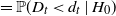 $=\mathbb{P}(D_{t} < d_{t}\mid H_{0})$
that falls below a predefined significance level
$=\mathbb{P}(D_{t} < d_{t}\mid H_{0})$
that falls below a predefined significance level
 $a\in(0,1)$
(e.g. 1%). This acceptance/rejection test seems to be more powerful than other classical tests, when the item under consideration exhibits random short-time malfunctions while most of the time it seems to operate normally. This can be easily justified because, in this case, it is likely that one or only a few of the durations
$a\in(0,1)$
(e.g. 1%). This acceptance/rejection test seems to be more powerful than other classical tests, when the item under consideration exhibits random short-time malfunctions while most of the time it seems to operate normally. This can be easily justified because, in this case, it is likely that one or only a few of the durations
 $X_{1},X_{2},\ldots,X_{Y_{t}+1}$
will be recorded as very short, while the rest of them will not exhibit a significant deviation from the null hypothesis. As a result, the classical test statistics (e.g. the mean duration time or the Kolmogorov–Smirnov statistic) may not be observed to be more extreme than the critical value, since they are not considerably affected by one or only a few short durations. On the contrary, a test based on the minimum duration seems more likely to correctly reject the null hypothesis.
$X_{1},X_{2},\ldots,X_{Y_{t}+1}$
will be recorded as very short, while the rest of them will not exhibit a significant deviation from the null hypothesis. As a result, the classical test statistics (e.g. the mean duration time or the Kolmogorov–Smirnov statistic) may not be observed to be more extreme than the critical value, since they are not considerably affected by one or only a few short durations. On the contrary, a test based on the minimum duration seems more likely to correctly reject the null hypothesis.
Hypothesis testing
The procedure described in the quality control example could be used more widely to examine whether the interarrival times of a renewal process
 $\{Y_{t},t\geq0\}$
are i.i.d. from a specific distribution F. For example, we can exploit this simple scheme to test the homogeneity of a Poisson process. In particular, we would like to test the null hypothesis
$\{Y_{t},t\geq0\}$
are i.i.d. from a specific distribution F. For example, we can exploit this simple scheme to test the homogeneity of a Poisson process. In particular, we would like to test the null hypothesis
 \begin{align*} H_{0}\colon\{Y_{t},t\geq0\}\text{ is a Poisson counting process with constant intensity }{\lambda}\end{align*}
versus the alternative hypothesis
 \begin{align*}H_{1}\colon\text{there exists a subinterval of }[0,t]\text{ where the intensity is higher than }{\lambda}.\end{align*}
It is obvious that, under
 $H_{1}$
, we may observe events in a certain subinterval more frequently than expected under
$H_{1}$
, we may observe events in a certain subinterval more frequently than expected under
 $H_{0}$
, leading to smaller observed spacings between them. Therefore, the null hypothesis could be rejected when the minimal observed spacing, say
$H_{0}$
, leading to smaller observed spacings between them. Therefore, the null hypothesis could be rejected when the minimal observed spacing, say
 $d_{t}$
, is significantly smaller than expected under
$d_{t}$
, is significantly smaller than expected under
 $H_{0}$
, i.e. when the p-value
$H_{0}$
, i.e. when the p-value
 $=\mathbb{P}(D_{t} < d_{t} \mid H_{0})$
is smaller than the significance level
$=\mathbb{P}(D_{t} < d_{t} \mid H_{0})$
is smaller than the significance level
 $a\in(0,1)$
of the test.
$a\in(0,1)$
of the test.
Acknowledgement
The author would like to thank the referees for their helpful comments and suggestions that improved the presentation and the quality of this paper.
Funding information
There are no funding bodies to thank relating to the creation of this article.
Competing interests
There were no competing interests to declare which arose during the preparation or publication process of this article.
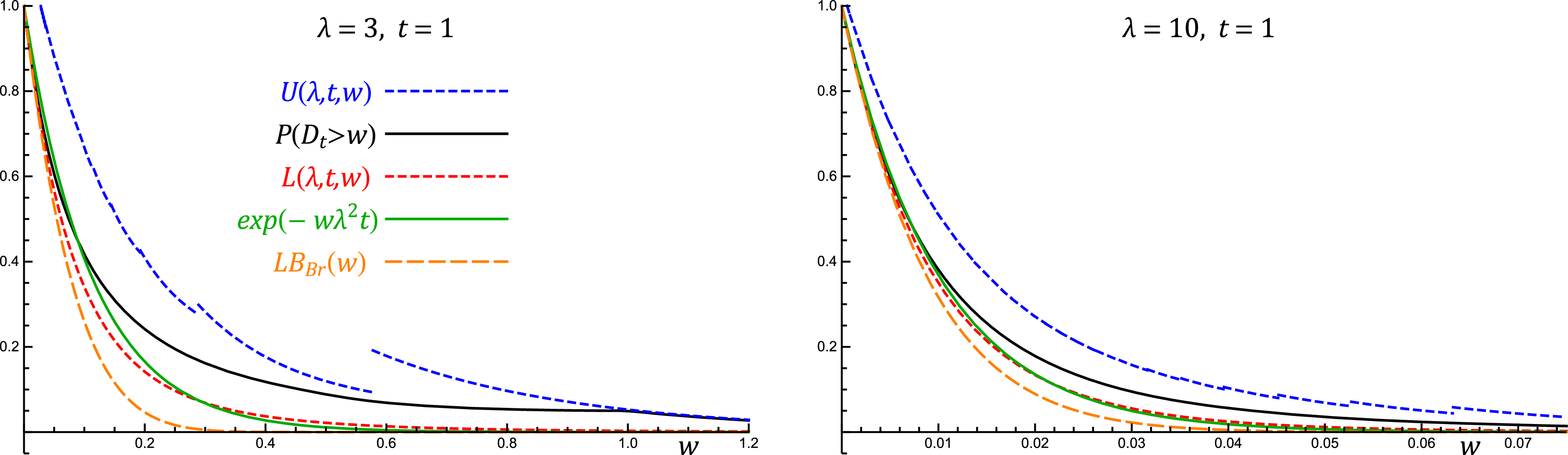

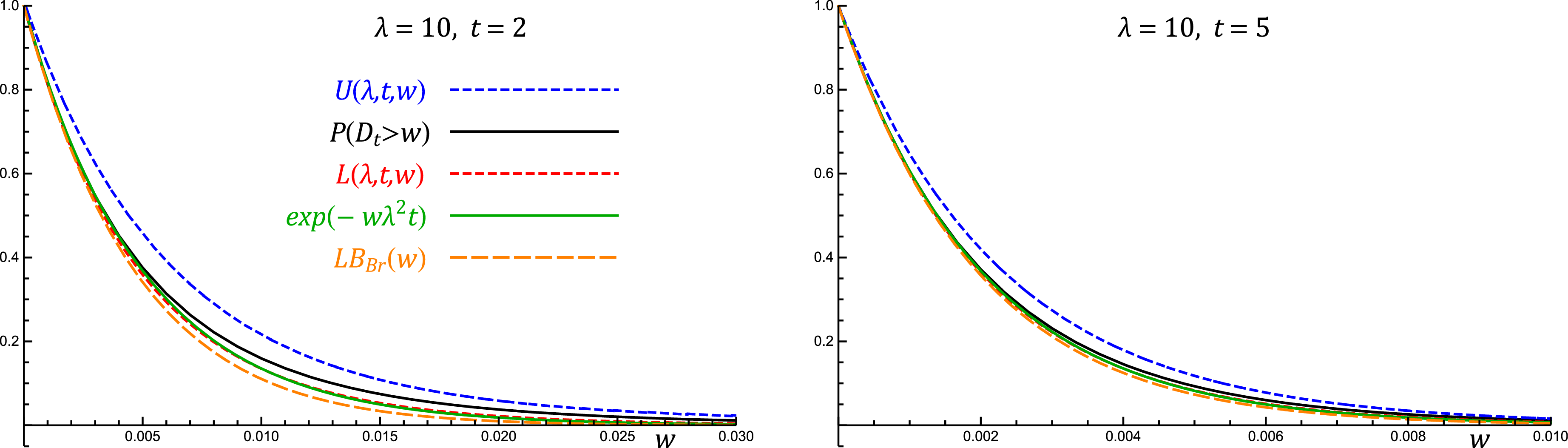


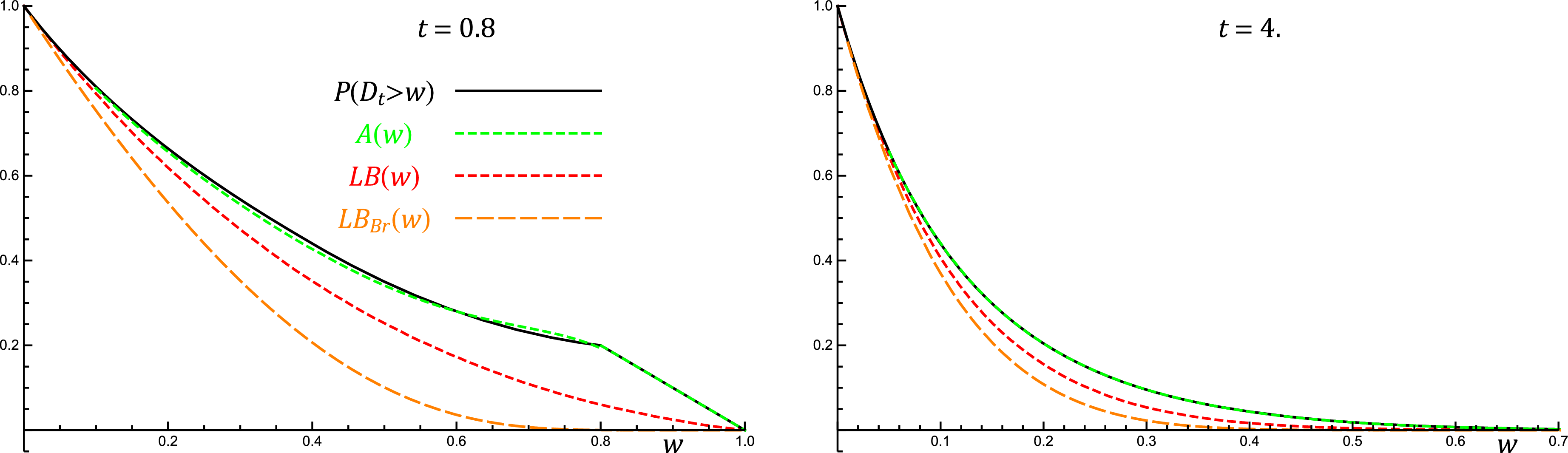


 Open access