Growing, Shrinking, and Long-Run Economic Performance: Historical Perspectives on Economic Development

Abstract

Although long-run economic performance has improved primarily through a decline in the rate and frequency of shrinking rather than through an increase in the rate of growing, most analysis of economic development has focused on increasing the rate of growing. We examine the forces making for a reduction in the rate of shrinking. The main proximate factors considered are (1) structural change, (2) technological change, (3) demographic change, and (4) stabilization policy. We conclude by considering institutions and institutional change as the key ultimate factors behind the reduction in shrinking, showing how they operate through political stability.

Understanding long-run economic performance is a fundamental concern of economists, economic historians, and social scientists more generally. To date, most work in this area has focused on “growing,” but recent work for the post-1950 period has suggested that economies vary at least as much in how they “shrink” as in how they grow (Easterly et al. 1993; Rodrik 1999; Pritchett 2000; Cuberes and Jerzmanowski 2009). However, despite these findings on the volatility of GDP per capita in poor countries, there has been little research into why poor societies shrink so often or by so much. Furthermore, economic historians have not so far systematically investigated the possibility that improved long-run economic performance during the late medieval period as well as since the eighteenth century could have been due to less shrinking rather than faster growing, despite the widespread acceptance of the idea that economic growth was at best slow before and during the Industrial Revolution (Crafts and Harley 1992; Broadberry et al. 2015). In this paper, we show that to understand economic performance over the long run, economic historians, growth economists, and development specialists need to explain a reduction in the rate and frequency of shrinking rather than an increase in the rate of growing, a different problem from the one they normally address.

The key empirical findings reported here can be summarized as follows, where the growing rate refers to the average rate of change only during years of positive growth and the shrinking rate refers to the average rate of change only during years of shrinking (i.e., negative growth): (1) In most of the world since 1950, and historically for today’s countries where data are available back to the thirteenth century, growing rates and shrinking rates have been high and variable. (2) When average growing rates have been high, average shrinking rates have also typically been high. Similarly, when average growing rates have been low, average shrinking rates have been low. (3) The improvement of economic performance over the long run has occurred primarily because the frequency and rate of shrinking have both declined, rather than because the growing rate has increased. (4) Indeed, as long-run economic performance has improved over time, the short-run rate of growing has normally declined rather than increased, but the frequency of growing has increased. In arithmetic terms, changes in growing rates by themselves would have led to lower rates of long-term economic growth, ceteris paribus. To avoid misunderstanding, however, it is important to be clear that we do not dispute in any way that positive long-run economic performance requires positive short-run growing and that increases in short-run growing rates contribute to positive long-run economic performance. Rather, we draw attention to the underappreciated role that economic shrinking has played both in the period since WWII and over the last millennium. The data and replication files can be downloaded from Broadberry and Wallis (2025).

Despite this important role for a reduction in the rate and frequency of shrinking in the transition to modern economic growth in today’s mature developed economies as well as in later developing countries, most analysis of the process of economic development has hitherto focused on increasing the rate of growing. Here, we make a start on redressing the balance by analyzing the forces making for a reduction in shrinking, drawing a distinction between proximate and ultimate factors. The main proximate factors considered are (1) structural change, (2) technological change, (3) demographic change, and (4) stabilization policy. Institutions and institutional change are seen as the key ultimate factors behind the reduction in shrinking, operating through political stability.

LONG- AND SHORT-RUN ECONOMIC PERFORMANCE

Economic Performance in the Contemporary World

We know that today’s high-income countries have had a better long-run economic performance than today’s low-income countries since at least the early nineteenth century (Maddison 2001, 2010). That fact is the essential motivation for growth theory, with its focus on the rate of growing. On closer examination, however, high-income countries do not grow faster during their episodes of positive growth than poor countries grow during their episodes of positive growth. This can be demonstrated using information from the Penn World Tables (PWT) for the period 1950–2011 (Feenstra, Inklaar, and Timmer 2015). Table 1 from PWT 8.0 provides evidence of long-run economic performance across groups of countries, broken down by level of income. The sample underlying the table includes 142 countries, with all included countries having data available from at least 1970 onwards. The data are arranged in five groups, ranging from high-income countries with per capita incomes in the year 2000 greater than $20,000 (in constant 2005 dollars) to poor countries with per capita incomes of less than $2,000.

Table 1 PENN WORLD TABLE 8.0: GROWING AND SHRINKING OF COUNTRIES BY INCOME CATEGORIES, 1950–2011

Notes: The “Real GDP per capita (Constant Prices: Chain series)” and their calculated annual growth rates for that series “Growth rate of Real GDP per capita (Constant Prices: Chain series)” were used to construct this table. Countries were first sorted into income categories based on their income in 2000, measured in 2005 dollars. Average annual positive and negative growth rates are the simple arithmetic average for all of the years and all of the countries in the income category without any weighting. The Penn World Table includes information on 167 countries. The sample runs from 1950 to 2011, although information is not available for every country in every year. Countries are included only where information is available at least as far back as 1970, resulting in a sample of 142 countries. Kuwait, Saudi Arabia, Qatar, Brunei, Oman, and Bahrain are excluded from the over $20,000 bin.

Source: Penn World Table 8.0, http://www.rug.nl/research/ggdc/data/pwt/pwt-8.0.

Table 1 makes use of an identity for establishing the contributions of growing and shrinking to long-run economic performance. Long-run economic performance can be measured by the rate of change of per capita GDP over periods of 50 years or longer. Economic performance over this time frame is the aggregation of short-run changes measured at the annual level. Long-run economic performance, g, is a combination of four factors: (1) the frequency with which an economy grows, f(+), (2) the rate at which it grows when growing, or the growing rate, g(+), (3) the frequency with which an economy shrinks, f(–), and (4) the rate at which it grows when shrinking, or the shrinking rate g(–). Thus:

g = {f(+) g(+)} + {f(–) g(–)} (1)

Since the frequency of growing is equal to one minus the frequency of shrinking, Equation (1) can be rewritten as:

g = {[1 – f(–)] g(+)} + {f(–) g(–)}, (2)

which reduces the number of independent factors to three. We can use this identity to decompose long-run economic performance into shrinking and growing components. We will show that better long-run economic performance occurred not so much because of an increase in the growing rate, but more because of a reduction in the rate and frequency of shrinking.

In Part A of Table 1, we see from the third column that poor countries have not grown less rapidly than rich countries when they have been growing. Indeed, the average growing rate has actually been higher for poorer countries than for richer countries. Similarly, we can see in the final column that the average shrinking rate has also been higher for poorer countries. However, the second column shows that the frequency of growing has been higher for countries with higher levels of per capita income. The richest countries grew in approximately 84 percent of years, while the poorest countries grew in just 63 percent of years. Since the frequency of shrinking is one minus the frequency of growing, the frequency of shrinking has to be higher for poorer countries: the poorest countries shrank in almost 37 percent of years, while the richest countries shrank in just 16 percent of years. So poor countries have grown less frequently than rich countries; they have higher shrinking rates and shrinking frequencies.

Part B of Table 1 shows the contributions of growing and shrinking to long-run economic performance. The contribution of growing to long-run economic performance is the growing rate multiplied by the frequency of growing years. We see that most poorer countries had a stronger contribution from growing than economies with per capita incomes above $20,000, since the higher average growing rate of poorer countries more than offset the lower frequency of growing years. The only exception to this was the poorest category of countries with per capita incomes below $2,000. These very poor countries had a weaker contribution of growing than the richest group of countries, but this was due to their lower frequency of growing years rather than to a lower growing rate. The contribution of shrinking to long-run economic performance is the shrinking rate multiplied by the frequency of shrinking years. All poorer economies had a bigger negative contribution from shrinking than economies with per capita incomes above $20,000. This was due to both the higher frequency of shrinking among poorer countries and higher shrinking rates.

The top three income groups experienced roughly the same annual net rate of change of real per capita income between 1950 and 2011, 2.8 to 3.0 percent, but the highest income group had a much lower contribution of growing and shrinking than the next two groups. Countries with incomes between $5,000 and $20,000 grew much faster when they grew and shrank much faster when they shrank than countries with incomes over $20,000, as can be seen in Table 1. The difference between the net rate of change in the poorest countries (0.85 percent) and the richest countries (2.83 percent) is 1.98 percent. The contribution of growing explains 36 percent of the difference in growth between the poorest and richest countries (=(3.19 – 2.48)/1.98), while the contribution of shrinking explains 64 percent (=(–0.37 – (–1.63))/1.98). That is what we mean by the statement that shrinking contributes more to the difference in the growth experience of poor countries relative to rich countries.

Long-run economic performance is measured by the net rate of change in per capita incomes in the final column of Table 1, Part B. Poorer economies did not have a significantly better long-run economic performance than the richest group of countries, which means that there was no systematic catching-up over the period as a whole. Middle-income countries increased their per capita incomes at about the same rate as the rich countries, but poor countries increased their per capita incomes substantially more slowly, so there was unconditional divergence rather than convergence as the poorest countries fell increasingly behind (Pritchett 1997).¹ This lack of long-run convergence is explained mainly by differences between countries in the contribution of shrinking, as rich countries shrank less and in fewer years than poor countries.

The next two sections explore the implications of the post-1950 findings for a longer sweep of economic history, encompassing the transition to modern economic growth in today’s rich countries. To do this, we make use of the Maddison Data Base for the nineteenth and twentieth centuries and data on a sample of four European countries for which annual data have recently become available, reaching back to the thirteenth century.

Economic Performance in the Nineteenth and Twentieth Centuries

For the nineteenth and twentieth centuries, we use annual data on 14 European countries starting between 1820 and 1870 and 4 New World economies starting in 1870 taken from the database left by Angus Maddison at the time of his death in March 2010 (Maddison 2010). Annual data for most other economies begin only in the twentieth century, and in many cases after 1950 (Maddison 2010). Although the Maddison Project has extended the series further into the twenty-first century and incorporated annual data for the pre-1820 period, the core nineteenth and twentieth-century elements of the database remain largely unchanged (Bolt and van Zanden 2014).² Part A of Table 2 shows data on the frequency of growing and shrinking for the 18-country sample as a whole, while figures are given for a number of individual countries in Appendix Table A1 for illustrative purposes. The frequency of growing has increased very sharply in the period since 1950 in this group of rich countries in Europe and the New World, or, to state it the other way round, there has been a sharp reduction in the frequency of shrinking, from about one-third to one-eighth.

Table 2 GROWING AND SHRINKING IN 18 EUROPEAN AND NEW WORLD COUNTRIES, 1820–2008

Notes: The included European countries are Britain, France, Italy, Belgium, the Netherlands, Switzerland, Austria, Germany, Portugal, Spain, Finland, Denmark, Norway, and Sweden. The four New World countries are the United States, Australia, New Zealand, and Canada.

Source: Derived from Maddison (2010).

Table 2B shows the average growth rate in all years, growing years, and shrinking years, that is, long-run economic performance, the growing rate, and the shrinking rate. Again, the data in the text table are provided for the 18-country sample as a whole, with data on some individual countries shown in Appendix Table A2 for illustrative purposes. Since 1950, the growth rate across all years has increased sharply in both Europe and the New World, and this has happened despite the fact that the growing rate (i.e., the growth rate in growing years) has actually fallen substantially almost everywhere.³ Long-run economic performance improved despite the reduction in the growing rate because of an even sharper decline in the shrinking rate combined with a reduction in the frequency of shrinking.

It should also be noted from Table 2B that during the period 1910–1950, covering the two World Wars and the Great Depression, the growing rate increased almost everywhere, in many cases substantially so.⁴ However, this did not lead to any significant improvement in long-run economic performance because there was an equally sharp increase in the shrinking rate, while the frequency of shrinking also increased slightly. It is natural to associate this increased volatility with the two world wars and the financial crises of the interwar period.

Table 2C shows how the frequency of growing and shrinking interacted with the growing and shrinking rates to produce the contributions of growing and shrinking to long-run economic performance, as measured by the average rate of change of per capita income in all years. Data on some individual countries are also shown in Appendix Table A3. Again, this makes clear that the improvement in economic performance during 1950–2008 compared with earlier periods can be attributed mainly to a reduction in the contribution of shrinking, since the contribution of growing either stagnated or actually declined slightly in most countries. The simple growing/shrinking comparison across the earliest and latest time periods, 1820–1870 and 1950–2008, from Table 2C shows that growing accounts for 21 percent of the increase in the rate of change of per capita income of 1.15 percent, from 1.40 in the early period to 2.55 in the later period, ((2.72 – 2.47)/(2.55 – 1.40)) while shrinking accounts for 79 percent of the increase ((–0.16 – (–1.08))/(2.55 – 1.40)). The reduction in the rate and frequency of shrinking is roughly four times more important than the increase in the rate and frequency of growing in the countries of the developed west between 1820 and 2008.

Economic Performance over the Very Long Run

Recent work in historical national accounting has extended annual estimates of GDP per capita as far back as the thirteenth or fourteenth centuries for a number of European countries (Broadberry 2022). We also analyze this Very Long Run Data Base for Britain, the Netherlands, Italy, and Spain (Broadberry et al. 2015, 2022; van Zanden and van Leeuwen 2012; Malanima 2011; Álvarez Nogal and Prados de la Escosura 2013). The annual time series are plotted in Figure 1A for Italy and Spain, in Figure 1B for Britain and the Netherlands, with the four countries being considered together in Figure 1C. Beginning with the Mediterranean economies in Figure 1A, there was a clear alternation of periods of positive and negative trend growth over periods of a decade or more, with growth booms typically followed by growth reversals, leaving little or no progress in the level of per capita incomes over the long run. Per capita GDP therefore fluctuated without a long-run trend before the nineteenth century. For the cases of Britain and the Netherlands in Figure 1B, however, although there were alternating periods of positive and negative growth until the eighteenth century, there was also a clear upward trend over the long run, with the gains following the Black Death being retained, and periods of negative growth becoming dampened with the transition to modern economic growth in the eighteenth century. As periods of negative growth became less frequent and as the rate of shrinking decreased in the North Sea area, Britain and Holland overtook Italy and Spain, as shown in Figure 1C.

Figure 1 REAL GDP PER CAPITA IN BRITAIN, THE NETHERLANDS, ITALY, AND SPAIN 1270–1870 (1990 INTERNATIONAL DOLLARS, LOG SCALE)

Sources: Malanima (2011), Álvarez-Nogal and Prados de la Escosura (2013), Broadberry et al. (2015, 2022), and van Zanden and van Leeuwen (2012).

(2015, 2022), van Zanden and van Leeuwen (2012), Malanima (2011), and Álvarez-Nogal and Prados de la Escosura (2013).

It is also useful to quantify the number of significant growing episodes (defined as at least three consecutive years of positive per capita GDP growth) and the number of shrinking episodes (defined as at least three consecutive years of negative per capita GDP growth). The results can be seen in Table 3, assessed over the long period 1348–1870 for which data are available covering all four countries. Notice that the number of growing episodes was higher in Italy than in both Britain and the Netherlands, while it was just as low in the Netherlands as in Spain, while the number of shrinking episodes in Britain and the Netherlands was lower than in both Mediterranean economies. The reversal of fortunes between the North Sea area and the Mediterranean economies thus occurred not because of a greater incidence of growing episodes in Britain and the Netherlands, but rather because of fewer shrinking episodes.

Table 3 SIGNIFICANT GROWING EPISODES (≥ 3 CONSECUTIVE YEARS OF POSITIVE PER CAPITA GDP GROWTH) AND SHRINKING EPISODES (≥ 3 CONSECUTIVE YEARS OF NEGATIVE PER CAPITA GDP GROWTH), 1348–1870

Sources: Derived from Broadberry et al. (2015, 2022), van Zanden and van Leeuwen (2012), Malanima (2011), and Álvarez-Nogal and Prados de la Escosura (2013).

However, a complete analysis must cover all years rather than just those with at least three consecutive years of growing or shrinking. Table 4 shows the frequency, rates, and contributions of growing and shrinking to long-run economic performance over complete periods of roughly 50 years in the Very Long Run Data Base, as in the analysis of the Penn World Table and the Maddison Data Base. The first thing to note from Table 4A is that for all of the economies considered here, the frequency of shrinking was about one-third in the nineteenth century, as in Table 2. For earlier centuries, by contrast, these economies grew and shrank in roughly equal proportions of years. A reduction in shrinking therefore played an important role in the improved long-run economic performance of Western Europe. Second, turning to Table 4B, we see that growing and shrinking rates tended to move together in absolute values, so that high rates of growing were accompanied by high rates of shrinking, and low rates of growing were accompanied by low rates of shrinking.⁵

Table 4 GROWING AND SHRINKING IN FOUR EUROPEAN COUNTRIES, 1270–1870

Sources: Derived from Broadberry et al. (2015, 2022), van Zanden and van Leeuwen (2012), Malanima (2011), and Álvarez-Nogal and Prados de la Escosura (2013).

Examining the British case in more detail, it is worth noting the critical juncture of the Industrial Revolution during the eighteenth century. The improvement in economic performance between 1700–1750 and 1750– 1800 was not in any way due to an increase in the contribution of growing. First, note that the frequency of growing increased very little from 52 to 54 percent (Table 4A). Second, the growing rate declined from 2.85 to 2.47 percent, a decrease of 0.38 percentage points, while the shrinking rate fell by a much larger amount from –2.78 to –1.98 percent, a change of –0.80 percentage points (Table 4B). The contribution of growing thus fell from 1.48 to 1.34 percent, or a decline of 0.14 percentage points, while the contribution of shrinking declined from –1.33 to –0.91 percent, raising economic performance by 0.42 percentage points (Table 4C). The net effect on overall economic performance was an increase from 0.15 to 0.43 percent, a change of 0.28 percentage points. Changes on the shrinking side thus more than explain the change in economic performance over this period, offsetting the negative effect of changes on the growing side.

A Summary of the Empirical Results

Before moving on to the explanatory section, it will be useful to summarize the main empirical results, which a framework for understanding long-run economic performance needs to be able to explain:

1. (1) Growing rates and shrinking rates have been high and variable throughout most of history and remain high and variable in less developed economies today.

2. (2) Improving long-run economic performance has occurred because the frequency and rate of shrinking have both declined, rather than because the growing rate has increased.

3. (3) The rate of growing usually declines rather than increases as countries begin to experience long-run modern economic growth.

WHY DO ECONOMIES STOP SHRINKING?

The previous section has established that the transition to sustained economic growth has historically owed more to a reduction in the rate and frequency of shrinking than to an increase in the rate of growing. Put simply, economic development depends on economies dampening growth reversals and ultimately reducing shrinking to persistently low levels. However, there has been no systematic analysis of shrinking episodes or of the reasons for their dampening and disappearance for much of the twentieth century, even after their return with a vengeance since 2008. Rather, shrinking episodes seem to be regarded as aberrant anomalies, caused by exogenous negative shocks.

Focusing on the Very Long Run Database, most previous accounts of the Industrial Revolution in Britain seek to explain an increase in the rate of growing rather than a reduction in the rate and frequency of shrinking. As Ashton’s [1948, p. 48] “wave of gadgets swept over England” during the eighteenth century, the average rate of growing during periods of positive growth was actually falling (Table 4B). But this still led to improved long-run economic performance because of a decline in the rate and frequency of shrinking. So it is not enough to explain why great inventors discovered coke smelting of iron or the spinning jenny in cotton textiles. We also need to understand why Britain and other parts of Europe stopped shrinking. After all, it has been known for some time that coke smelting of iron was widely used in Northern Song China, seven hundred years before Abraham Darby rediscovered it at Coalbrookdale (Hartwell 1966). And as Allen (2009, pp. 904–7) has pointed out, inventions such as the spinning jenny were so simple in principle that they were almost bound to be discovered once people started looking for them. And yet researchers continue to focus on innovation during periods of positive growth, while the issue of why economies shrink continues to be largely ignored.

So why have the frequency and rate of shrinking declined as economies have made the transition to long-run modern economic growth? In addressing this question, we follow Maddison (1991, p. 12) in drawing a distinction between proximate and ultimate elements explaining per capita GDP performance, but focusing on shrinking rather than growing. The main proximate factors considered here are (1) structural change, (2) technological change, (3) demographic change, and (4) stabilization policy. None of these factors appears to explain much, if any, of the decline in shrinking over the long sweep of history considered here. We then turn to the more fundamental causes of the decline in shrinking, arguing that institutional structure should be considered as a key ultimate factor behind the reduction in shrinking.

PROXIMATE CAUSES OF THE DECLINE IN SHRINKING

Structural Change

The period 1270–1870 saw a major structural shift of the British economy away from agriculture, which accounted for around 40 percent of nominal GDP between the late fourteenth century and the end of the sixteenth century, declining to around 30 percent during the seventeenth and eighteenth centuries, and around 20 percent by the mid-nineteenth century (Broadberry et al. 2015, p. 194). Short-run fluctuations of agricultural output were often extremely large, with annual declines of 10 or 20 percent a frequent occurrence, as weather-related shocks led regularly to bad harvests and years of shrinking. As the share of agriculture in overall economic activity declined, therefore, it may be expected that such episodes of shrinking would become less important.

However, we are interested in changes in the balance between growing and shrinking, and a reduction in the importance of a more volatile sector such as agriculture may in fact be expected to affect the growing rate just as much as the shrinking rate, so that it may not end up having a large effect on long-run economic performance. It is useful, therefore, to consider the contributions of growing and shrinking at a sectoral level. Table 5A shows the frequency, average rates of change, and unweighted contributions of growing and shrinking in each sector for the period 1270–1348, while Table 5B shows the magnitudes of the same variables for the period 1800–1870. Comparing these two panels, we see that there was only a very small change in the frequency of shrinking in agriculture between 1270–1348 and 1800–1870 (from 47 to 49 percent). This contrasts with substantial declines in the frequency of shrinking in both industry (from 44 to 29 percent) and services (from 27 to 20 percent).

Table 5 SHIFT-SHARE ANALYSIS OF THE CONTRIBUTION OF AGRICULTURE TO BRITISH ECONOMIC PERFORMANCE

Source: Derived from Broadberry et al. (2015).

Tables 5A and 5B also set out the average rates of change of output in growing and shrinking years and across all years in both periods.

In agriculture, both the growing and shrinking rates declined, with the shrinking rate declining by more than the growing rate, leading to improved economic performance across all years. Services also exhibited an improvement in output performance across all years, but with an increase in both the growing and shrinking rates. Industry is the most dynamic sector, with an improvement across all years resulting from a combination of an increase in the growing rate and a decline in the shrinking rate. Tables 5A and 5B also show how the frequencies and rates of growing and shrinking interacted to determine the contributions of growing and shrinking to long-run economic performance, measured as the average rate of change of output in all years. Again, all sectors showed an improved long-run economic performance, but industry stands out as the only sector where the contribution of growing increased and the contribution of shrinking declined. In agriculture, the contributions of growing and shrinking both declined, while in services the contributions of growing and shrinking both increased.

The question of the extent to which the declining share of agriculture might explain the decline in shrinking rates and frequencies in the aggregate economy is addressed directly in Tables 5C and 5D. These tables perform shift-share analysis for the periods 1270–1348 and 1800–1870, respectively. The first column of Tables 5C and 5D sets out the shares of output in agriculture, industry, and services in 1381, the earliest bench-mark year for which shares of nominal GDP are available (Broadberry et al. 2015, p. 194). At this point, agriculture accounted for more than 45 percent of British GDP. The second column of Tables 5C and 5D sets out the shares in 1841, when agriculture’s share had fallen to just over 22 percent. Table 5C then shows the effect of weighting the contributions of growing and shrinking from Table 5A with first the 1381 sectoral shares and then with the 1841 sectoral shares. If the declining share of agriculture is what mattered for improved economic performance at the aggregate level, then shifting from the use of 1381 weights to 1841 weights with the same unweighted contributions in each sector should have a significant effect on economic performance across all years. However, this is clearly not the case for the 1270–1348 period, where switching to the 1841 weights increases the rate of change across all years from 0.16 to just 0.18 percent. Similarly for the 1800–1870 period, in Table 5D, shifting from the 1841 weights with a small agricultural sector to the 1381 weights with a much larger agricultural sector has only a modest effect on the overall rate of change across all years, decreasing it from 2.07 to 1.74 percent. In practice, then, the declining share of agriculture between 1270–1348 and 1800–1870 explains rather less than might be expected of the patterns of growing, shrinking, and economic performance that are observed in the data. Conversely, developments within each of the individual sectors, including agriculture, were of rather more importance.

Technological Change

In theory, shrinking could disappear as the economy moves from technological stagnation to technological progress. In a world with no technological progress, an upturn must lead to positive per capita GDP growth, while a downturn must lead to negative growth, that is, shrinking. It is tempting to think that the emergence of trend technological progress for the first time could therefore lead to the elimination of shrinking, with downturns now having only slower per capita GDP growth. However, there is an obvious problem with this argument. Imagine that the entire distribution of growing and shrinking episodes shifts a fixed amount towards growing. Shrinking rates and frequencies would both decline, in line with the theory. However, growing rates and frequencies should both increase, so that there is an increase in the contribution of growing as well as a decrease in the contribution of shrinking. We have, however, already seen that this is inconsistent with the historical or contemporary data on economic performance. Although the contribution of shrinking did decline during the transition to modern economic growth the contribution of growing also declined. In particular, since the frequency of growing increased, there was a substantial decline in the rate of growing, which would be hard to characterize as the result of an acceleration in the rate of technological progress.

However, we can also tackle this issue in a more empirical way, by checking whether, in practice, the scale of technological progress at the time of the transition to modern economic growth was large enough to explain the declining shrinking rates and frequencies that we observe. To do this, we examine trend growth in total factor productivity (TFP) growth. The main constraint in measuring TFP growth in the past is the lack of reliable data on the capital stock. For Britain, however, Feinstein’s (1988) estimates back to 1760 have been produced using the perpetual inventory method, ensuring consistency between the stock of capital and the flows of investment. The augmented Solow growth accounting estimates of Crafts (1995), shown in Table 6, derive TFP growth taking into account the growth of human capital as well as raw labor and physical capital. As annual output growth accelerated from 0.60 percent during 1760–1780 to reach a peak of 2.40 percent during 1831–1873, TFP growth increased only from 0.05 to 0.35 percent. TFP growth therefore accounted for just one-sixth of the increase in output growth, with five-sixths of the increase being accounted for by faster growth of factor inputs.

Table 6 ACCOUNTING FOR BRITISH GDP GROWTH, 1760–1913 (PERCENT PER ANNUM)

Notes: The factor weights are 0.4 for capital, 0.35 for labor, and 0.25 for human capital.

Source: Crafts (1995, p. 752).

Estimates of TFP growth for Holland are provided by van Zanden and van Leeuwen (2012), covering the period 1540–1800 and including human capital as well as labor and capital inputs. In Table 7, Dutch TFP is estimated using the same weights as those used by Crafts and Harley (1992) for Britain (0.4 for capital, 0.35 for labor, and 0.25 for human capital). These estimates differ only very slightly from those of van Zanden and van Leeuwen, who also include land as a fourth-factor input. The period of fastest TFP growth was 1540–1620, during the Dutch Golden Age, at 0.64 percent per annum. This was higher than at any other time in Holland during the seventeenth and eighteenth centuries or in Britain during the eighteenth and nineteenth centuries, but was still relatively small compared with the average growing and shrinking rates for the Netherlands in Table 4B. Furthermore, this period of positive TFP growth was followed by a period of strongly negative TFP growth between 1620 and 1665 and barely positive TFP growth thereafter, so there was no trend increase in TFP over the period 1540–1800 as a whole. The Dutch example thus serves as a reminder that growth reversals can occur in TFP as well as GDP per capita, and that the transition to modern economic growth requires an end to TFP growth reversals as well as GDP per capita growth reversals.

Table 7 ACCOUNTING FOR DUTCH GDP GROWTH, 1540–1800 (PERCENT PER ANNUM)

Notes: The factor weights are 0.4 for capital, 0.35 for labor, and 0.25 for human capital.

Source: Derived from van Zanden and van Leeuwen (2012, p. 126).

Demographic Change

The Malthusian approach explains the long-run stagnation of GDP per capita in the pre-industrial world with shorter episodes of growing and shrinking through demographic factors (Malthus 1798; Clark 2007). Malthus assumed feedback from income per capita to fertility (the preventive check) and mortality (the positive check), together with diminishing returns to land (the resource constraint). Short-run growing of per capita income occurs in response to anything that reduces population (an increase in mortality or a decline in fertility) or increases the availability of land. Short-run shrinking of per capita income occurs in response to a decline in mortality, an increase in fertility, or a reduction in the availability of land. In the Malthusian approach, however, any gain to GDP per capita will only be temporary because of the feedback from living standards to fertility and mortality.

As noted earlier, the growth in living standards in Italy after the Black Death of the mid-fourteenth century, and its subsequent reversal after the return to population growth from the mid-fifteenth century, can be understood in the light of the Malthusian model. However, other countries do not fit into this approach at all well. Most obviously, Britain and the Netherlands were able to break free during the early modern period from the Malthusian constraints that held Italy on a path of long-run stagnation, despite similar demographic trends. As the population returned to its pre-Black Death level in Britain and Holland during the sixteenth and seventeenth centuries, Holland enjoyed its Golden Age of economic growth,while British living standards remained on a plateau rather than declining.For England,excellent demographic data exist for the period since 1541, as the result of a major research project by Wrigley and Schofield (1981), and can be considered alongside the GDP per capita data examined in the second section of this paper. Figure 2 provides a graph of annual data on the crude birth rate and the crude death rate per 1,000 population. It is immediately clear that England’s breaking out of the Malthusian trap in the eighteenth century was not caused by a reduction in fertility or an increase in mortality. Indeed, there was a population explosion after 1750 as fertility increased substantially while mortality declined (Wrigley and Schofield 1981, pp. 314–15). Furthermore, when the fertility transition did begin in England with the decline in the crude birth rate from the 1870s, there was a decline in economic performance. The fertility decline from the 1870s can be seen clearly for England in Figure 2 and applies also to the rest of Britain (Tranter 1996, p. 86). The decline in economic performance shows up in the GDP per capita growth rate for the United Kingdom in Table A2 and is conventionally referred to as the late Victorian climacteric (Matthews, Feinstein, and Odling-Smee 1982).

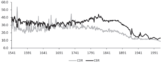
Figure 2 VITAL RATES IN ENGLAND 1541–2000 (CRUDE BIRTH RATE AND CRUDE DEATH RATE PER 1,000 POPULATION)

Sources: Wrigley and Schofield (1981), Mitchell (1988), and U.K. National Statistics Office (2004a), Annual Abstract of Statistics.

Spain provides another interesting example of an economy behaving in a non-Malthusian way after the Black Death. In contrast to Italy, the Netherlands, and Britain, Spain did not experience even a temporary increase in per capita incomes after the Black Death. Álvarez-Nogal and Prados de la Escosura (2013) explain this by the high land-to-labor ratio in a frontier economy during the Reconquest. Instead of reducing pressure on scarce land resources, the Spanish population decline destroyed commercial networks and further isolated an already scarce population, reducing specialization and the division of labor. Thus Spain did not share in the general West European increase in per capita incomes after the Black Death. This serves as a useful reminder that the mechanical operation of demographic forces highlighted in the Malthusian approach can be offset and dominated by the forces of coordination emphasized in the Smithian approach. Explaining the changing relationship between population, output, and per capita output has proved difficult enough in unified growth theory, even abstracting from the issue of shrinking (Galor and Weil 2000; Galor 2005).

Stabilization Policy

We have already noted that the contribution of shrinking declined substantially from around 1950. During the 1950s and 1960s, it was widely believed that the absence of shrinking, leading to the attainment of full employment across much of the world, could be attributed to the Keynesian revolution, as a result of governments adopting macroeconomic stabilization policies. As Matthews (1968) pointed out, if this really were the case, it would be a remarkable thing, since it would mean that this most striking feature of the postwar world would be due to an advance in economic theory. Matthews went on to suggest that full employment could be attributed to an investment boom after the war, which he thought had little if anything to do with Keynesian fiscal policies.

In addition to the work by Matthews, detailed studies of the relationship between fiscal policy and economic activity in Britain suggested that postwar fiscal policy was, if anything, destabilizing. Dow (1964, pp. 178–213) examined in some detail the effect of tax changes on both consumption and investment between 1945 and 1960, noting the difficulties of assessing the current state of the economy and forecasting where it was likely to be when the policies took effect, given lags in the process, particularly when considering the effects on investment. He concluded that “the major variations of fiscal policy were in fact not stabilizing, but rather themselves one of the main causes of instability; and that demand would have remained much more nearly in balance with supply if fiscal policy had, throughout the period, been less actively interventionist” (Dow 1964, p. 211). In a follow-up study of the period 1960–1974, Price (1979, p. 216) concluded that “budgetary policy had exerted a procyclical influence; indeed, fluctuations in the economy would have been reduced if budgetary leverage had not fluctuated.”

These pessimistic evaluations of the postwar stabilization policy are reflected in the negative correlation (R = –0.3) between the constant employment budget balance (CEBB) and the annual growth rate of investment (GFCF) in Figure 3. When there was a boom in gross fixed capital formation, there was a tendency for the constant employment budget balance to worsen, indicating a decline in tax revenue relative to government expenditure or a pro-cyclical boost to economic activity. With the disappearance of full employment across the Western world from the 1970s, the idea that the adoption of Keynesian stabilization policies was responsible for the sharp reduction in shrinking during the postwar period appeared less plausible, and economists increasingly used evidence on fiscal stance and macroeconomic volatility to make the case for restricting fiscal policy discretion (Fatás and Mihov 2003; Battilossi, Foreman-Peck, and Kling 2010).

Figure 3 CONSTANT EMPLOYMENT BUDGET BALANCE AND GROSS FIXED CAPITAL FORMATION GROWTH IN THE UNITED KINGDOM, 1949–1977

Sources: Constant employment budget balance: Ward and Neild (1978). GFCF growth derived from U.K. National Statistics Office (2004b), Economic Trends Annual Supplement.

ULTIMATE CAUSES OF THE DECLINE IN SHRINKING

Institutions and Economic Development

There is no doubt that governments are an important source of institutions and institutional change, and a natural corollary to economic instability is political instability. Table 1 puts countries into income bins. Table 8 uses the Penn World Table data, Version 9, and sorts countries into eight equal-size income octile bins for the period 1960 to 2015. The upper panel of the table includes an unbalanced sample of 164 countries for which we have data in 2010, while the balanced lower panel is restricted to the 93 countries that are in the sample continuously from 1960 to 2010. The 21 countries in the eighth octile of the upper panel, the richest countries, are essentially the developed countries in the OECD (which is why we chose octile bins). The third column of Table 8 also includes data on “adverse political events” taken from a number of sources. In the Archigos data set, any change of executive leaders results in a “regime change.” A “regular” regime change occurs when leadership transitions under existing agreed-upon rules, such as an election in the United States or the succession of a hereditary monarch by his son. An “irregular” regime change occurs as the result of a coup, a civil war, or any other change that does not follow existing agreed-upon rules. Irregular regime transitions are adverse political events (Goemans, Gleditsch, and Chiozza 2009). Political events also include new constitutions from the Comparative Constitutions data set (Elkins and Ginsburg 2022). Political events in the table mark a significant change in the leadership and/or change in the structure of a government. In institutional terms, an adverse political event signals a change in the rules. Whether for better or worse is, in this case, inconsequential.

Table 8 RATES OF CHANGE OF PER CAPITA INCOME AND FREQUENCY OF ECONOMIC AND POLITICAL INSTABILITY SORTED BY INCOME

Notes: The number of countries taken into account for statistics in Panel A is 164, and in Panel B it is 93. In Panel A, the first octile corresponds to the poorest 12.5 percent of the countries according to incomes in 2010, while in Panel B it corresponds to the poorest 12.5 percent of the countries according to incomes in 1960.

Sources: Penn World Table 9.0, Archigos Dataset (Goemans, Gleditsch, and Chiozza 2009), and Comparative Constitutions Project (Elkins and Ginsburg 2022).

Table 9 RATES OF CHANGE OF PER CAPITA INCOME AND FREQUENCY OF ECONOMIC INSTABILITY SORTED BY INCOME

Notes: The number of countries taken into account for statistics in Panel A is 164, and in Panel B it is 93. In Panel A, the first octile corresponds to the poorest 12.5 percent of the countries according to incomes in 2010, while in Panel B the first octile corresponds to the poorest 12.5 percent of the countries according to incomes in 1960.

Source: Penn World Table 9.0.

One of the striking features of Table 1 is the variation across the income bins in the rate of shrinking. The high-income countries shrink at a rate of –2.32 percent, while countries in the four poorer bins all shrink at –4.21 percent or higher in absolute terms. This pattern is more emphatic in Table 9, wherein the upper panel shows that all seven of the poorest octiles have shrunk near to or greater than –4.0 percent and the richest octile has a shrinking rate of only –1.97 percent. A shrinking rate of half of the poorer countries combined with a shrinking frequency slightly less than half of the frequencies in the poorer countries is, as we have shown in the paper, the major difference between economic performance in the “developed” world and the rest of the world. Extended periods of low shrinking rates are rare but not unknown over the long stretch of history recounted in Panel B of Table 4, where only three out of the possible 43 country time periods have an average shrinking rate of less than –2 percent and an additional four time periods with shrinking rates between –2 percent and –2.5 percent. As we noted, periods of low shrinking rates tend to be associated with periods where growing rates are also low.

What about political stability? The third column of Table 8 gives the frequency of adverse political events by income level. In both panels there is a steady, but not quite monotonic decline in the frequency of political instability. As a simple measure of stability, political stability appears more highly correlated with real per capita income than economic stability. The frequency of shrinking, the fifth column of Table 9, is essentially flat from income octiles three to seven, while the frequency of political events declines as income rises. In the late twentieth century, societies with more stable governments tended to have higher levels of per capita income. However, higher per capita income with more stable governments does not produce more stable economies across the middle five-eighths of the country distribution. The exception is the very highest income octile: essentially the 18 European and New World countries represented in Table 2.

From 1960 to 2010, the richest 21 countries in the world experienced almost no political instability, as defined here.⁶ The Archigos data span the years from 1875 to 2015 and 168 countries. There are 3,406 incidents of regime change in the data set. The incidents are taken from histories, and the histories of countries in the developed world are richer, and for much of the period from 1875 to 1960 or so, many countries in the world were colonies with little or no control over their governing regime. Still, it is interesting to compare the sample of 18 countries included in Table 2 to the rest of the world.

Table 10 breaks the sample into three groups. Information on regimes is divided into the conditions on the entry of the regime (primarily regular or irregular) and conditions on the exit of the regime (see the note to the table). An elected regime following the electoral rules but displaced by a coup would have a “regular entry” and an “irregular exit.” The first column gives the total number of regimes in the 18 countries included in Table 2, amounting to 844 regimes from 1875 to 2015. Of those 844 regimes, there are 14 irregular entries (2 percent) and 32 irregular exits (4 percent). Among the irregular exits were the governments displaced by the German invasion after 1939, numerous events in Spain and Portugal (15 of the 32 irregular exits), and four assassinations, three in the United States and one in Sweden.

Table 10 REGULAR AND IRREGULAR REGIME CHANGES IN 18 COUNTRIES AND THE REST OF THE WORLD

Notes: Irregular exits in the original data include “Natural Deaths,” “Retired due to Illness,” “Suicide,” and “Still in Office.” These have been removed from the irregular exits here. Remaining irregular exits include “Removed by Military, without Foreign Support,” “Removed by Military, with Foreign Support,” ”Removed through Threat of Foreign Force,” “Assassination by Unsupported Individual,” “Popular Protest, with Foreign Support,” “Removed by Other Government Actors, with Foreign Support,” “Removed by Other Government Actors, without Foreign Support,” “Removed by Rebels, with Foreign Support,” “Removed by Rebels, without Foreign Support,” “Removed in Military Power Struggle Short of Coup,” and “Unknown.” Sources: Archigos Dataset (Goemans, Gleditsch, and Chiozza 2009).

The second column of Table 10 gives the total number of regimes in the rest of the world for the whole period 1875–2015. There were 2,565 regimes in total. Irregular entry accounted for 599 (23 percent) of regime entries and irregular exit accounted for 640 (25 percent) of all regime exits. The third column gives the rest of the world total from 1960 to 2015, in case post-colonial independence had a significant effect on regime entry and exit, but it seems not to have done so. There were 1,446 regimes, of which irregular entry occurred in 291 cases (20 percent) and irregular exit occurred in 287 cases (20 percent). The post-1960 regimes were not more likely to experience irregular entries or exits than the entire rest of the world from 1875 to 2015; indeed, the share of irregular regime changes was a bit higher before 1960 than after.

Unlike the numbers in Tables 1, 8, and 9, these are not frequencies of regime change, but the share of all regime changes that are regular or irregular. In the developed world, governing regimes change with regularity following the established rules and procedures. In the rest of the world, the developing countries, irregular regime changes occur frequently: between a fifth and a quarter of the time. Most irregular regime changes are the result of domestic issues. The largest category of irregular exits is “Removed by Military, without foreign support”: 273 of the 599 cases of irregular exits. In only 58 of the 599 cases is “foreign support” indicated. These are societies that find it difficult to come to internal agreements about the common rules, the institutions, which people agree to through a collective process. That is inherently an institutional problem.

Political and Economic Stability

The preceding section illuminates the political side of a history of shrinking. It is the political component of a history every economic historian is familiar with. In the late nineteenth and early twentieth centuries, the economies of a small number of countries, no more than 20, began growing at modern rates of somewhere between 1 and 1.5 percent per year in real per capita income. Those countries were located in Northwestern Europe and four English-speaking former British colonies. They remain the richest societies in the world today. All of the 18 countries whose growth experience is reflected in Table 2 adopted some elements of democracy in the nineteenth century. Even Spain attempted elections with universal male suffrage in several constitutions. Democracy failed in five of the countries in the 1920s and 1930s, leading to an extremely costly world war. Germany, Austria, and Italy recovered their democracies under the control of the Allied powers after the war and began to recover economically. Spain and Portugal remained autocracies for longer and suffered economically for longer as well. In the 1950s and 1960s, a strong case could be made that democracy led to or perhaps even caused economic development, as all the wealthy countries had democracies, and the two that failed to regain their democracies, Spain and Portugal, were falling behind.

Subsequent history has complicated the picture, however. After the collapse of colonialism in the 1960s, the selection of leaders through elections, the simplest form of democracy, spread throughout the world in the manner of Huntington’s (1991) waves. Today, roughly three-quarters of the nations in the world have at least some minimal form of democracy, and by no means have they all made the transition to modern economic growth. Since all of the developed societies are also advanced democracies, there is clearly a connection between some aspects of democracy and more stable polities, but it is not clear which aspects of democracy are critical to enhancing stability, what the connections are, or how they operate.

The numbers presented in this paper suggest that “stability,” however defined, is an important source of growth. Societies that are able to reduce the variability of both political and economic outcomes appear to be the ones that grow and develop first and fastest. The “however defined” qualifier is important. If we define stability in terms of the variance of growth rates over time in a society, then a mean-preserving narrowing of the variance will not affect long-term growth rates. What happened in the developed world was an asymmetric reduction in the variance of annual growth, which we have documented, in which the long-term growth-enhancing effects came primarily from reducing the negative growth experiences, rather than a shift in growth outcomes that left the shape of the distribution of outcomes largely unchanged.

CONCLUSIONS

We have shown in simple arithmetic terms that the onset of modern economic growth is quantitatively the result of less frequent and less rapid shrinking of real per capita GDP more than it is due to a rise in the rate of economic growth when economies are growing. A decline in the shrinking frequency, as we have defined it, is automatically an increase in the growing frequency. The combined effects of the shrinking frequency and shrinking rate explain a significantly larger share of the improved economic performance in the developed, rich societies of the contemporary world than the combined effects of the growing frequency and growing rate. Likewise, the high frequency and rates of economic shrinking in the rest of the world are important reasons why poor countries are poor, all along the country income distribution.

While we do not wish to deny the importance of structural, demographic, or technological change on the level of economic performance over time, we believe that these long-run sources of growth do not explain fundamentally the changing patterns of short-run economic performance that, over time, make up the long-term trends. While there is wide agreement that institutions are an important source of economic growth and development, it is not clear how institutions affect stability. North (1990, pp. 3, 6) began Institutions, Institutional Change and Economic Performance with the following statements: “Institutions reduce uncertainty by providing a structure to everyday life. They are a guide to human interaction” and “The major role of institutions in a society is to reduce uncertainty by establishing a stable (but not necessarily efficient) structure to human interaction.” North’s intuition that institutions matter for economic performance because they reduce uncertainty by inducing stability resonates with the evidence presented in this paper. That economic growth is an increase in the productivity of individuals in the aggregate is a definition rather than an explanation. Combining intuition and definition has led economists and social scientists to focus on the uncertainty facing individuals making choices about investments in physical, human, and institutional capital, for example, secure property rights and the rule of law. However, the institutions that enable individuals to increase their productivity must themselves be stable to promote growth.

It is not that the stability of institutional arrangements has been ignored, but it has received far less attention in the economics and economic history literature than what makes for good institutions in terms of productivity. We need to better understand why most societies do not or cannot reach collective agreements—social, political, or economic—that are more stable over time. Unstable societies seem to be the rule, and the stable, developed societies of the present are very much the exception. The rich, stable countries are all advanced democracies, but democratic elections alone have not proven to generate stability or growth. North, Wallis, and Weingast (2009) suggested that it was the adoption of impersonal rules for forming organizations that was the key to modern development. Lamoreaux and Wallis have pushed the suggestion further, building on the fact that impersonal rules for many government functions (more than just for forming organizations) are a common institutional element in all of the advanced democracies, and in all of those societies impersonal rules were closely associated with the emergence of consolidated political parties and more stable political outcomes.⁷

We draw two conclusions. First, economic historians should be paying as much attention to what determines stability as to what determines growth. Second, our institutional analyses should likewise focus more on what enables social arrangements to be stable over time and relatively less on why particular institutional arrangements, like secure property rights, make individuals more productive. In other words, institutions may be an important source of economic stability and therefore of growth and development, but not the kind of economic institutions that economic history has, to date, focused on. It is time we thought more deeply about stability.