


1. Introduction
Joint transforms involving quantities associated with stopping times play a crucial role in the development of numerous risk models in actuarial science and financial mathematics. The most common stopping time in actuarial literature is the time until ruin, $\tau ,$
in a finite or infinite horizon. The ruin problem has been studied by many researchers in the last decades, providing closed-form formulae, for example, for the probability of the ultimate ruin. We refer to Willmot and Woo (Reference Willmot and Woo2017) for a recent review on ruin models.
$\tau ,$
in a finite or infinite horizon. The ruin problem has been studied by many researchers in the last decades, providing closed-form formulae, for example, for the probability of the ultimate ruin. We refer to Willmot and Woo (Reference Willmot and Woo2017) for a recent review on ruin models.
In addition to the probability of ruin, other quantities of interest in ruin theory are usually based on the surplus before ruin, $U_{\tau -},$
the deficit at ruin,
$U_{\tau -},$
the deficit at ruin, $-U_{\tau }$
, and the time until ruin,
$-U_{\tau }$
, and the time until ruin, $\tau$
. One of the most celebrated joint transforms involving these quantities was introduced by Gerber and Shiu (Reference Gerber and Shiu1998). After the publication of their work, a large number of papers appeared in the literature studying the so-called Gerber–Shiu discounted penalty function and its generalizations. The joint density of the pair
$\tau$
. One of the most celebrated joint transforms involving these quantities was introduced by Gerber and Shiu (Reference Gerber and Shiu1998). After the publication of their work, a large number of papers appeared in the literature studying the so-called Gerber–Shiu discounted penalty function and its generalizations. The joint density of the pair $(U_{\tau -},-U_{\tau })$
was also studied by Dickson (Reference Dickson1992). A simplistic assumption in these models is that the inter-claim times,
$(U_{\tau -},-U_{\tau })$
was also studied by Dickson (Reference Dickson1992). A simplistic assumption in these models is that the inter-claim times, $T$
, and claims sizes,
$T$
, and claims sizes, $X$
, are independent. In the last two decades, more realistic models involving the concept of dependence between claim sizes and inter-claim times started to attract the interest of many researchers, especially after the work of Albrecher and Boxma (Reference Albrecher and Boxma2004). There is strong real-world evidence and practical motivation for incorporating dependence (mostly positive) between inter-claim times and claim sizes in insurance risk modeling. In many instances, the magnitude of a claim tends to increase when a long time passes until it is reported, due to the accumulation of damages. For example, a vehicle that has not undergone maintenance for an extended time period may require significantly higher repair costs when eventually serviced, implying a positive dependence structure. Positive dependence also emerges in the context of catastrophic events, where shorter inter-claim times (i.e., high claim frequency after a large-scale event like a flood, earthquake, or hurricane) are usually associated with smaller individual claims (e.g., home insurance claims for minor damage). Conversely, longer waiting times may correspond to larger, isolated claims unrelated to catastrophic events. Furthermore, policyholders may intentionally delay filing a claim until the accumulated cost justifies doing so, reinforcing this dependence pattern. In this context, a large number of publications employ specific bivariate distributions that describe the dependence structure of the pair
$X$
, are independent. In the last two decades, more realistic models involving the concept of dependence between claim sizes and inter-claim times started to attract the interest of many researchers, especially after the work of Albrecher and Boxma (Reference Albrecher and Boxma2004). There is strong real-world evidence and practical motivation for incorporating dependence (mostly positive) between inter-claim times and claim sizes in insurance risk modeling. In many instances, the magnitude of a claim tends to increase when a long time passes until it is reported, due to the accumulation of damages. For example, a vehicle that has not undergone maintenance for an extended time period may require significantly higher repair costs when eventually serviced, implying a positive dependence structure. Positive dependence also emerges in the context of catastrophic events, where shorter inter-claim times (i.e., high claim frequency after a large-scale event like a flood, earthquake, or hurricane) are usually associated with smaller individual claims (e.g., home insurance claims for minor damage). Conversely, longer waiting times may correspond to larger, isolated claims unrelated to catastrophic events. Furthermore, policyholders may intentionally delay filing a claim until the accumulated cost justifies doing so, reinforcing this dependence pattern. In this context, a large number of publications employ specific bivariate distributions that describe the dependence structure of the pair $(T,X)$
. Boudreault et al. (Reference Boudreault, Cossette, Landriault and Marceau2006) considered the classical compound Poisson risk model, where the conditional distribution of the claim sizes was assumed to be a special mixture of two arbitrary distributions, and derived the Laplace transform (LT) of the Gerber–Shiu function in terms of the Dickson–Hipp operator. Albrecher and Teugels (Reference Albrecher and Teugels2006) considered several dependence structures for
$(T,X)$
. Boudreault et al. (Reference Boudreault, Cossette, Landriault and Marceau2006) considered the classical compound Poisson risk model, where the conditional distribution of the claim sizes was assumed to be a special mixture of two arbitrary distributions, and derived the Laplace transform (LT) of the Gerber–Shiu function in terms of the Dickson–Hipp operator. Albrecher and Teugels (Reference Albrecher and Teugels2006) considered several dependence structures for $(T,X)$
based on specific copulas and bivariate distributions, obtaining finite and infinite horizon ruin probabilities using Wiener–Hopf factorization. Cossette et al. (Reference Cossette, Marceau and Marri2008) derived a formula for the LT of the Gerber–Shiu discounted penalty function using a generalized FGM copula for
$(T,X)$
based on specific copulas and bivariate distributions, obtaining finite and infinite horizon ruin probabilities using Wiener–Hopf factorization. Cossette et al. (Reference Cossette, Marceau and Marri2008) derived a formula for the LT of the Gerber–Shiu discounted penalty function using a generalized FGM copula for $(T,X)$
with exponential marginals. Badescu et al. (Reference Badescu, Cheung and Landriault2009) offered explicit expressions for certain Gerber–Shiu discounted penalty functions depending only on the deficit at ruin, when the pair
$(T,X)$
with exponential marginals. Badescu et al. (Reference Badescu, Cheung and Landriault2009) offered explicit expressions for certain Gerber–Shiu discounted penalty functions depending only on the deficit at ruin, when the pair $(T,X)$
follows a bivariate phase-type distribution. Ambagaspitiya (Reference Ambagaspitiya2009) provided explicit formulae for the ultimate ruin probability using Wiener–Hopf factorization in two specific bivariate gamma distributions for
$(T,X)$
follows a bivariate phase-type distribution. Ambagaspitiya (Reference Ambagaspitiya2009) provided explicit formulae for the ultimate ruin probability using Wiener–Hopf factorization in two specific bivariate gamma distributions for $(T,X)$
. Zang et al. (Reference Zhang, Yang and Yang2012) considered finite mixtures of bivariate exponentials and derived an explicit expression for the Gerber–Shiu function. Chadjiconstantinidis and Vrontos (Reference Chadjiconstantinidis and Vrontos2014) studied the discounted joint and marginal distribution functions of
$(T,X)$
. Zang et al. (Reference Zhang, Yang and Yang2012) considered finite mixtures of bivariate exponentials and derived an explicit expression for the Gerber–Shiu function. Chadjiconstantinidis and Vrontos (Reference Chadjiconstantinidis and Vrontos2014) studied the discounted joint and marginal distribution functions of $U_{\tau -}$
and
$U_{\tau -}$
and $-U_{\tau }$
using the LT of the Gerber–Shiu function when the dependence of
$-U_{\tau }$
using the LT of the Gerber–Shiu function when the dependence of $(T,X)$
is described by the FGM copula with Erlang and exponential marginals for
$(T,X)$
is described by the FGM copula with Erlang and exponential marginals for $T$
and
$T$
and $X$
, respectively. Zhang and Li (Reference Zhang and Li2019) studied the distribution of discounted aggregate claims in a compound renewal risk model when the dependence between
$X$
, respectively. Zhang and Li (Reference Zhang and Li2019) studied the distribution of discounted aggregate claims in a compound renewal risk model when the dependence between $T$
and
$T$
and $X$
is modeled using a generalized FGM copula. More recently, Adékambi and Takouda (Reference Adékambi and Takouda2022) extended the work of Chadjiconstantinidis and Vrontos (Reference Chadjiconstantinidis and Vrontos2014) by adding a diffusion term to the surplus process, considering the same dependence structure for
$X$
is modeled using a generalized FGM copula. More recently, Adékambi and Takouda (Reference Adékambi and Takouda2022) extended the work of Chadjiconstantinidis and Vrontos (Reference Chadjiconstantinidis and Vrontos2014) by adding a diffusion term to the surplus process, considering the same dependence structure for $(T,X)$
. For a surplus process perturbed by diffusion, Li et al. (Reference Li, Sendova and Yang2024) considered a causal dependence structure between the inter-arrival time of the upcoming claim and the preceding claim size. For similar results in ruin theory involving dependence structures between the upcoming inter-claim time and the preceding claim size, see Mandjes and Boxma (Reference Mandjes and Boxma2023). For a brief overview of general bivariate distributions, we refer to Lai and Balakrishnan (Reference Lai and Balakrishnan2009).
$(T,X)$
. For a surplus process perturbed by diffusion, Li et al. (Reference Li, Sendova and Yang2024) considered a causal dependence structure between the inter-arrival time of the upcoming claim and the preceding claim size. For similar results in ruin theory involving dependence structures between the upcoming inter-claim time and the preceding claim size, see Mandjes and Boxma (Reference Mandjes and Boxma2023). For a brief overview of general bivariate distributions, we refer to Lai and Balakrishnan (Reference Lai and Balakrishnan2009).
A fruitful technique to compute quantities associated with the time until ruin is based on an appropriate change of the probability measure using likelihood ratio identities (see, for instance, Asmussen & Albrecher, Reference Asmussen and Albrecher2010). Under this new measure, which is constructed using roots of Lundberg-type equations, several quantities associated with the stopping time until ruin can alternatively be expressed via simpler formulae, for example, depending only on the distribution of the deficit at ruin. Schmidli (Reference Schmidli1995) offered approximations for ruin time probabilities employing a renewal model perturbed by diffusion via a change of measure technique. Schmidli (Reference Schmidli2010) studied the Gerber–Shiu discounted penalty function, assuming independent $T$
,
$T$
, $X$
, and managed to express this function in terms of an appropriate change of measure, without the presence of the discounted factor. Boutsikas et al. (Reference Boutsikas, Rakitzis and Antzoulakos2016) considered a Sparre-Andersen renewal risk model, with
$X$
, and managed to express this function in terms of an appropriate change of measure, without the presence of the discounted factor. Boutsikas et al. (Reference Boutsikas, Rakitzis and Antzoulakos2016) considered a Sparre-Andersen renewal risk model, with $T$
and
$T$
and $X$
independent and mixed Erlang distributed, and provided joint generating functions (GF) for the number of claims and the value of the surplus until it falls below zero or terminates above an upper safety level. These functions were expressed in terms of the distribution of the overshoot and the undershoot under an appropriately tilted measure. Boutsikas et al. (Reference Boutsikas, Economides and Vaggelatou2024) generalized the previous work incorporating a diffusion term and taking also into account the time and the total claim amount, until the double barrier stopping rule.
$X$
independent and mixed Erlang distributed, and provided joint generating functions (GF) for the number of claims and the value of the surplus until it falls below zero or terminates above an upper safety level. These functions were expressed in terms of the distribution of the overshoot and the undershoot under an appropriately tilted measure. Boutsikas et al. (Reference Boutsikas, Economides and Vaggelatou2024) generalized the previous work incorporating a diffusion term and taking also into account the time and the total claim amount, until the double barrier stopping rule.
Several generalizations of the Gerber–Shiu discounted penalty function have also been proposed in the last two decades. Cheung et al. (Reference Cheung, Landriault, Willmot and Woo2010) analyzed the Gerber–Shiu function taking into the account the surplus immediately prior to ruin, the deficit at ruin, the minimum surplus before ruin, and the surplus immediately after the second to last claim before ruin, under the presence of dependence between $T$
and
$T$
and $X$
. Frostig et al. (Reference Frostig, Pitts and Politis2012) studied an extension of the Gerber–Shiu function containing the number of claims until ruin, when the inter-claim times are Erlang distributed, independent of the claim sizes. Cossette et al. (Reference Cossette, Larrivée-Hardy, Marceau and Trufin2015) studied a generalization of the Gerber–Shiu function, including the minimum of the surplus before ruin, by employing the change of measure technique, and considered several dependent structures where the importance sampling method can be applied. For a review of Gerber–Shiu functions along with their generalizations, we refer to the recent review work of He et al. (Reference He, Kawai, Shimizu and Yamazaki2023). Moreover, many articles in the literature investigate the distribution of the number of claims until ruin, under the assumption of independence between
$X$
. Frostig et al. (Reference Frostig, Pitts and Politis2012) studied an extension of the Gerber–Shiu function containing the number of claims until ruin, when the inter-claim times are Erlang distributed, independent of the claim sizes. Cossette et al. (Reference Cossette, Larrivée-Hardy, Marceau and Trufin2015) studied a generalization of the Gerber–Shiu function, including the minimum of the surplus before ruin, by employing the change of measure technique, and considered several dependent structures where the importance sampling method can be applied. For a review of Gerber–Shiu functions along with their generalizations, we refer to the recent review work of He et al. (Reference He, Kawai, Shimizu and Yamazaki2023). Moreover, many articles in the literature investigate the distribution of the number of claims until ruin, under the assumption of independence between $(T,X)$
; see for example, Landriault et al. (Reference Landriault, Shi and Willmot2011), Frostig et al. (Reference Frostig, Pitts and Politis2012), Dickson (Reference Dickson2012), Zhao and Zhang (Reference Zhao and Zhang2013), Boutsikas et al. (Reference Boutsikas, Rakitzis and Antzoulakos2016), and Dickson (Reference Dickson2019). To the best of our knowledge, there are no published results yet for the distribution of the number of claims until ruin in the case of dependence between
$(T,X)$
; see for example, Landriault et al. (Reference Landriault, Shi and Willmot2011), Frostig et al. (Reference Frostig, Pitts and Politis2012), Dickson (Reference Dickson2012), Zhao and Zhang (Reference Zhao and Zhang2013), Boutsikas et al. (Reference Boutsikas, Rakitzis and Antzoulakos2016), and Dickson (Reference Dickson2019). To the best of our knowledge, there are no published results yet for the distribution of the number of claims until ruin in the case of dependence between $T$
,
$T$
, $X$
.
$X$
.
The aim of this paper is to propose a generalization of the Gerber–Shiu function that incorporates the number of claims until ruin in the case of dependence between the claim sizes and the inter-claim times. Using an appropriate change of measure technique, we present in Section 2 a general connection between already studied Gerber–Shiu functions and the proposed generalized one (cf. Corollary 2). We also offer a result connecting a special form of the Gerber–Shiu function with only the distribution of the deficit at ruin under the new measure (cf. Proposition 3). We further employ our general results to investigate two cases of bivariate distributions where we were able to extract closed-form formulae for the quantities of interest. More specifically, in Section 3, we employ a Downton–Moran bivariate exponential distribution to describe the dependence structure of our model, and we offer explicit formulae for some cases of the Gerber–Shiu functions that include the number of claims until ruin (cf. Proposition 6). In addition, we derive a closed formula for the defective discounted joint density of the number of claims until ruin, the deficit at ruin, and the time until ruin (cf. Proposition 9). The same is achieved for the joint density of the number of claims and the deficit at ruin (cf. Corollary 10). In Section 4, we generalize the results of the previous section by assuming that the inter-claim times and the claim sizes follow a Kibble–Moran bivariate Erlang distribution (cf. Proposition 14, Corollary 16). Finally, in the last section, we offer numerical examples in order to illustrate our main results.
2. The dependent renewal risk model
In a probability space $(\Omega ,\mathcal{F},\mathbb{P})$
, we consider the surplus process of the form
$(\Omega ,\mathcal{F},\mathbb{P})$
, we consider the surplus process of the form
 \begin{equation} U_{t}\,:\!=\, u+ct-\sum _{j=1}^{N_{t}}X_{j},\,\,\,t\geq 0, \end{equation}
where $u\geq 0$
denotes the initial surplus,
$u\geq 0$
denotes the initial surplus, $N=(N_{t},t\geq 0)$
is a renewal process,
$N=(N_{t},t\geq 0)$
is a renewal process, $X_{j},j=1,2,\ldots$
denote the claim sizes and
$X_{j},j=1,2,\ldots$
denote the claim sizes and $c\gt 0$
is the constant premium rate. We also denote by
$c\gt 0$
is the constant premium rate. We also denote by $T_{1},T_{2},\ldots$
the inter-claim times of the process
$T_{1},T_{2},\ldots$
the inter-claim times of the process $N,$
and by
$N,$
and by $Y_{k}\,:\!=\,\sum _{i=1}^{k}T_{i}$
the arrival time of the
$Y_{k}\,:\!=\,\sum _{i=1}^{k}T_{i}$
the arrival time of the $k$
-th claim. The non-negative random variables (RVs)
$k$
-th claim. The non-negative random variables (RVs) $T_{i}$
and
$T_{i}$
and $X_{i}$
may be dependent, while the pairs
$X_{i}$
may be dependent, while the pairs $(T_{1},X_{1})$
,
$(T_{1},X_{1})$
, $(T_{2},X_{2})$
,… are independent and identically distributed (IID) with common joint cumulative distribution function
$(T_{2},X_{2})$
,… are independent and identically distributed (IID) with common joint cumulative distribution function $F_{T,X}$
. Since the ruin event occurs only at claim arrival times
$F_{T,X}$
. Since the ruin event occurs only at claim arrival times $Y_{1},Y_{2},\ldots$
, the process
$Y_{1},Y_{2},\ldots$
, the process $(U_{t},t\geq 0)$
can be considered only at claim arrival times, and thus, for our exposition, it suffices to study the discrete time process
$(U_{t},t\geq 0)$
can be considered only at claim arrival times, and thus, for our exposition, it suffices to study the discrete time process $S=(S_{k},k=1,2,\ldots )$
, with
$S=(S_{k},k=1,2,\ldots )$
, with
 \begin{equation} S_{k}\,:\!=\, U_{Y_{k}}=u+cY_{k}-\sum _{j=1}^{k}X_{j}=u+\sum _{j=1}^{k}\left (cT_{j}-X_{j}\right )=u+\sum _{j=1}^{k}Z_{j} \end{equation}
where $Z_{j}\,:\!=\, cT_{j}-X_{j}$
, for every
$Z_{j}\,:\!=\, cT_{j}-X_{j}$
, for every $j=1,2,\ldots$
. Let
$j=1,2,\ldots$
. Let $\nu \,:\!=\,\inf \left \{ k\,:\,S_{k}\lt 0\right \}$
be the stopping time that counts the number of claims until the process
$\nu \,:\!=\,\inf \left \{ k\,:\,S_{k}\lt 0\right \}$
be the stopping time that counts the number of claims until the process $S$
drops below zero (ultimate ruin event) and
$S$
drops below zero (ultimate ruin event) and $\tau \,:\!=\, Y_{\nu }$
the total time until ruin. Obviously,
$\tau \,:\!=\, Y_{\nu }$
the total time until ruin. Obviously, $S_{\nu }=U_{\tau },\nu =N_{\tau }$
. Focusing on the process
$S_{\nu }=U_{\tau },\nu =N_{\tau }$
. Focusing on the process $S$
, we define a new measure on the measurable space
$S$
, we define a new measure on the measurable space $(\Omega ,\mathcal{F})$
, to be denoted by
$(\Omega ,\mathcal{F})$
, to be denoted by $\mathbb{P}_{h,\delta }$
, via the following martingale likelihood process
$\mathbb{P}_{h,\delta }$
, via the following martingale likelihood process
 \begin{equation*} L_{k}\,:\!=\,\frac {e^{\sum _{i=1}^{k}\left (\left (ch-\delta \right )T_{i}-hX_{i}\right )}}{\mathbb{M}_{T,X}\left (ch-\delta ,-h\right )^{k}},\;\;\;k=1,2,\ldots \end{equation*}
for two real parameters $\delta ,h$
such that
$\delta ,h$
such that $\mathbb{M}_{T,X}\left (ch-\delta ,-h\right )\lt \infty$
, where
$\mathbb{M}_{T,X}\left (ch-\delta ,-h\right )\lt \infty$
, where $\mathbb{M}_{T,X}\left (t,x\right )\,:\!=\,\mathbb{E}(e^{tT_{i}+xX_{i}})$
is the joint moment generating function (MGF) of
$\mathbb{M}_{T,X}\left (t,x\right )\,:\!=\,\mathbb{E}(e^{tT_{i}+xX_{i}})$
is the joint moment generating function (MGF) of $\left (T,X\right ).$
In particular, for every
$\left (T,X\right ).$
In particular, for every $A\in \mathcal{F}_{n}\,:\!=\,\sigma \left (\left \{ \left (T_{i},X_{i}\right ),i\leq n\right \} \right )\subseteq \mathcal{F}$
, we set
$A\in \mathcal{F}_{n}\,:\!=\,\sigma \left (\left \{ \left (T_{i},X_{i}\right ),i\leq n\right \} \right )\subseteq \mathcal{F}$
, we set
 \begin{equation*} \mathbb{P}_{h,\delta }\left (A\right )\,:\!=\,\mathbb{E}\left (1_{A}L_{n}\right ). \end{equation*}
The measures $\mathbb{P}$
and
$\mathbb{P}$
and $\mathbb{P}_{h,\delta }$
are equivalent, and under
$\mathbb{P}_{h,\delta }$
are equivalent, and under $\mathbb{P}_{h,\delta }$
, the MGF of
$\mathbb{P}_{h,\delta }$
, the MGF of $Z_{1}$
is given by
$Z_{1}$
is given by
 \begin{equation} \mathbb{E}_{h,\delta }\big(e^{tZ_{1}}\big)=\mathbb{E}\left (e^{t\left (cT_{1}-X_{1}\right )}\frac {e^{\left (\left (ch-\delta \right )T_{1}-hX_{1}\right )}}{\mathbb{M}_{T,X}\left (ch-\delta ,-h\right )}\right )=\frac{\mathbb{M}_{T,X}(c(t+h)-\delta ,-(t+h))}{\mathbb{M}_{T,X}(ch-\delta ,-h)}. \end{equation}
It is worth stressing that this new measure can be considered as an exponential tilting measure affecting the joint distribution of $T_{i},X_{i}$
(i.e., it is a bivariate Esscher transform), while it is easy to verify that the pairs
$T_{i},X_{i}$
(i.e., it is a bivariate Esscher transform), while it is easy to verify that the pairs $(T_{1},X_{1})$
,
$(T_{1},X_{1})$
, $(T_{2},X_{2})$
, … remain IID under
$(T_{2},X_{2})$
, … remain IID under $\mathbb{P}_{h,\delta }$
. A fundamental result of this work is the following theorem, where, by exploiting this change of measure technique, we offer an identity that can be used to generalize existing GS functions. An RV
$\mathbb{P}_{h,\delta }$
. A fundamental result of this work is the following theorem, where, by exploiting this change of measure technique, we offer an identity that can be used to generalize existing GS functions. An RV $W$
will be called
$W$
will be called $\mathcal{F}_{\nu }$
-measurable if, for every
$\mathcal{F}_{\nu }$
-measurable if, for every $k\in \mathbb{N},$
the RV
$k\in \mathbb{N},$
the RV $W1_{[\nu =k]}$
is
$W1_{[\nu =k]}$
is $\mathcal{F}_{k}$
-measurable.
$\mathcal{F}_{k}$
-measurable.
Theorem 1.
If there exists a real function $\gamma =\gamma _{z,\delta }$
such that
$\gamma =\gamma _{z,\delta }$
such that
 \begin{equation} z\mathbb{M}_{T,X}\left (c\gamma -\delta ,-\gamma \right )=1, \end{equation}
then for every $\mathcal{F}_{\nu }$
-measurable RV
$\mathcal{F}_{\nu }$
-measurable RV $W$
, the following identity holds
$W$
, the following identity holds
 \begin{equation} \mathbb{E}\left (z^{\nu }e^{-\delta \tau }W1_{[\tau \lt \infty ]}\right )=e^{\gamma u}\mathbb{\mathbb{E}}_{\gamma ,\delta }\left (e^{-\gamma U_{\tau }}W1_{[\tau \lt \infty ]}\right ), \end{equation}
for all $\gamma ,\delta ,z\in \mathcal{R}$
such that the above expectations exist.
$\gamma ,\delta ,z\in \mathcal{R}$
such that the above expectations exist.
Proof.
Let $V$
be any
$V$
be any $\mathcal{F}_{\nu }$
-measurable RV. We have that
$\mathcal{F}_{\nu }$
-measurable RV. We have that
 \begin{equation*} \mathbb{E}\left(Ve^{h\left (S_{\nu }-u\right )-\delta Y_{\nu }}1_{[\nu \lt \infty ]}\right )=\sum _{k=1}^{\infty }\mathbb{E}\Big(V1_{[\nu =k]}e^{h\sum _{j=1}^{k}Z_{j}-\delta \sum _{j=1}^{k}T_{j}}\Big). \end{equation*}
For every $k\geq 1$
, the RV
$k\geq 1$
, the RV $V_{k}=V1_{[\nu =k]}$
is
$V_{k}=V1_{[\nu =k]}$
is $\mathcal{F}_{k}$
-measurable and therefore
$\mathcal{F}_{k}$
-measurable and therefore
 \begin{equation*} \frac{\mathbb{E}\big(V1_{[\nu =k]}e^{h\sum _{j=1}^{k}Z_{j}-\delta \sum _{j=1}^{k}T_{j}}\big)}{\mathbb{M}_{T,X}\left (ch-\delta ,-h\right )^{k}}=\frac {\mathbb{E}\big(V_{k}e^{\sum _{i=1}^{k}\left (\left (ch-\delta \right )T_{i}-hX_{i}\right )}\big)}{\mathbb{M}_{T,X}(ch-\delta ,-h)^{k}}=\mathbb{E}\left (V_{k}L_{k}\right )=\mathbb{\mathbb{E}}_{h,\delta }\left (V_{k}\right ). \end{equation*}
Hence,
 \begin{eqnarray}\mathbb{E}\left (Ve^{h\left (S_{\nu }-u\right )-\delta Y_{\nu }}1_{[\nu \lt \infty ]}\right ) & = &\sum _{k=1}^{\infty }\mathbb{E}\Big(V1_{[\nu =k]}e^{h\sum _{j=1}^{k}Z_{j}-\delta \sum _{j=1}^{k}T_{j}}\Big)\nonumber\\& =&\sum _{k=1}^{\infty }\mathbb{\mathbb{E}}_{h,\delta }\big(V1_{[\nu =k]}\mathbb{M}_{T,X}\left (ch-\delta ,-h\right )^{k}\big)\nonumber \\ & = &\mathbb{\mathbb{E}}_{h,\delta }\left (V\mathbb{M}_{T,X}\left (ch-\delta ,-h\right )^{\nu }1_{[\nu \lt \infty ]}\right ). \end{eqnarray}
For $h=\gamma$
such that
$h=\gamma$
such that $z\mathbb{M}_{T,X}\left (c\gamma -\delta ,-\gamma \right )=1$
, we get
$z\mathbb{M}_{T,X}\left (c\gamma -\delta ,-\gamma \right )=1$
, we get
 \begin{equation*} \mathbb{E}\big(Ve^{\gamma \left (S_{\nu }-u\right )-\delta Y_{\nu }}1_{[\nu \lt \infty ]}\big)=\mathbb{\mathbb{E}}_{\gamma ,\delta }\left (Vz^{-\nu }1_{[\nu \lt \infty ]}\right ). \end{equation*}
Applying the above to the $\mathcal{F}_{\nu }$
-measurable RV
$\mathcal{F}_{\nu }$
-measurable RV $V=z^{\nu }e^{-\gamma \left (S_{\nu }-u\right )}W$
and taking into account the fact that
$V=z^{\nu }e^{-\gamma \left (S_{\nu }-u\right )}W$
and taking into account the fact that $S_{\nu }=U_{\tau },Y_{\nu }=\tau$
and
$S_{\nu }=U_{\tau },Y_{\nu }=\tau$
and $1_{[\nu \lt \infty ]}=1_{[\tau \lt \infty ]}$
a.s., we get the desired result.
$1_{[\nu \lt \infty ]}=1_{[\tau \lt \infty ]}$
a.s., we get the desired result.
We can now exploit Theorem1 in order to reduce the form of Gerber–Shiu functions (see Gerber & Shiu, Reference Gerber and Shiu1998), which also contain the number of claims until ruin, $\nu ,$
by expressing them under the new measure
$\nu ,$
by expressing them under the new measure $\mathbb{P}_{\gamma ,\delta }$
. We offer the following corollary for any penalty function
$\mathbb{P}_{\gamma ,\delta }$
. We offer the following corollary for any penalty function $w\left (U_{\tau -},-U_{\tau }\right )$
of the surplus prior to ruin and the deficit at ruin.
$w\left (U_{\tau -},-U_{\tau }\right )$
of the surplus prior to ruin and the deficit at ruin.
Corollary 2. The generalized GS function satisfies the following identity
 \begin{equation*} \phi (u)\,:\!=\,\mathbb{E}\Big(z^{\nu }e^{-\delta \tau }\,w\left (U_{\tau -},-U_{\tau }\right )1_{[\tau \lt \infty ]}\Big)=e^{\gamma u}\mathbb{E}_{\gamma ,\delta }\left (e^{-\gamma U_{\tau }}w\left (U_{\tau -},-U_{\tau },\right )1_{[\tau \lt \infty ]}\right ), \end{equation*}
where $\gamma =\gamma _{z,\delta }$
is a real root of the generalized Lundberg equation (
2.4
) and
$\gamma =\gamma _{z,\delta }$
is a real root of the generalized Lundberg equation (
2.4
) and $\delta$
represents the constant discount rate.
$\delta$
represents the constant discount rate.
Proof.
Setting as $W$
the function
$W$
the function $w\left (U_{\tau -},-U_{\tau }\right )$
, which obviously is an
$w\left (U_{\tau -},-U_{\tau }\right )$
, which obviously is an $\mathcal{F}_{\nu }$
-measurable function, the formula (2.5) leads to the above identity.
$\mathcal{F}_{\nu }$
-measurable function, the formula (2.5) leads to the above identity.
The above form of the GS function (in the special case where $z=1$
) is considered by Badescu et al. (Reference Badescu, Cheung and Landriault2009) and Cossette et al. (Reference Cossette, Marceau and Marri2008).
$z=1$
) is considered by Badescu et al. (Reference Badescu, Cheung and Landriault2009) and Cossette et al. (Reference Cossette, Marceau and Marri2008).
It is worth mentioning that the above corollary could similarly be formulated employing alternative penalty functions, for example, depending on the last minimum of the surplus before ruin, $\underline {U}_{\tau -}\,:\!=\,\inf \{U_{t},t\lt \tau \}$
, the surplus on the second to last claim before ruin,
$\underline {U}_{\tau -}\,:\!=\,\inf \{U_{t},t\lt \tau \}$
, the surplus on the second to last claim before ruin, $U_{Y_{\nu -1}}$
, etc. (e.g., see Woo, Reference Woo2010). We refer to the review paper of He et al. (Reference He, Kawai, Shimizu and Yamazaki2023) for a list of cases for GS penalty functions.
$U_{Y_{\nu -1}}$
, etc. (e.g., see Woo, Reference Woo2010). We refer to the review paper of He et al. (Reference He, Kawai, Shimizu and Yamazaki2023) for a list of cases for GS penalty functions.
In what follows, we denote by
 \begin{equation*} \mathbb{B}_{h,\delta }\left (t\right )\,:\!=\,\mathbb{E}_{h,\delta }\big(e^{t(-U_{\tau })}\mid \tau \lt \infty\big) \end{equation*}
the MGF of the deficit at ruin, under the measure $\mathbb{P}_{h,\delta }$
. In the following proposition, we present an identity that enables us to explicitly express a special case of the GS function, namely, the joint GF of the number of claims until ruin, the deficit at ruin, and the time until ruin. We further denote by
$\mathbb{P}_{h,\delta }$
. In the following proposition, we present an identity that enables us to explicitly express a special case of the GS function, namely, the joint GF of the number of claims until ruin, the deficit at ruin, and the time until ruin. We further denote by $\psi _{h,\delta }\,:\!=\,\mathbb{P}_{h,\delta }\left (\tau \lt \infty \right )$
the ruin probability under
$\psi _{h,\delta }\,:\!=\,\mathbb{P}_{h,\delta }\left (\tau \lt \infty \right )$
the ruin probability under $\mathbb{P}_{h,\delta }$
.
$\mathbb{P}_{h,\delta }$
.
Proposition 3.
If there exists a real function $\gamma =\gamma _{z,\delta }$
such that
$\gamma =\gamma _{z,\delta }$
such that $z\mathbb{M}_{T,X}\left (c\gamma -\delta ,-\gamma \right )=1$
, then
$z\mathbb{M}_{T,X}\left (c\gamma -\delta ,-\gamma \right )=1$
, then
 \begin{equation} \phi _{z,\delta ,s}(u)\,:\!=\,\mathbb{E}(z^{\nu }e^{-sU_{\tau }-\delta \tau }1_{[\tau \lt \infty ]})=\psi _{\gamma ,\delta }\,e^{\gamma u}\mathbb{B}_{\gamma ,\delta }\left (\gamma +s\right ), \end{equation}
for all $s,\delta ,z\in \mathcal{R}$
such that the above expectations exist. In addition, the probability of the ultimate ruin
$s,\delta ,z\in \mathcal{R}$
such that the above expectations exist. In addition, the probability of the ultimate ruin $\psi \,:\!=\,\mathbb{P}\left (\tau \lt \infty \right )$
is given by
$\psi \,:\!=\,\mathbb{P}\left (\tau \lt \infty \right )$
is given by
 \begin{equation*} \psi =\psi _{\gamma ^{*},0}\,e^{\gamma ^{*}u}\mathbb{B}_{\gamma ^{*},0}\left (\gamma ^{*}\right ), \end{equation*}
where $\gamma ^{*}\,:\!=\,\gamma _{1,0}$
is a real root of the equation
$\gamma ^{*}\,:\!=\,\gamma _{1,0}$
is a real root of the equation $\mathbb{M}_{T,X}\left (c\gamma ^{*},-\gamma ^{*}\right )=1$
.
$\mathbb{M}_{T,X}\left (c\gamma ^{*},-\gamma ^{*}\right )=1$
.
Proof.
Using Theorem1 for $W=e^{-sU_{\tau }}$
, the r.h.s. of Equation (2.5) becomes
$W=e^{-sU_{\tau }}$
, the r.h.s. of Equation (2.5) becomes
 \begin{align*} e^{\gamma u}\mathbb{\mathbb{E}}_{\gamma ,\delta }\left (e^{-\gamma U_{\tau }}e^{-sU_{\tau }}1_{[\tau \lt \infty ]}\right ) & =e^{\gamma u}\mathbb{\mathbb{E}}_{\gamma ,\delta }\left (\left .e^{\left (\gamma +s\right )\left (-U_{\tau }\right )}\right |\tau \lt \infty \right )\mathbb{P}_{\gamma ,\delta }\left (\tau \lt \infty \right )\\ & =\psi _{\gamma ,\delta }e^{\gamma u}\mathbb{B}_{\gamma ,\delta }\left (\gamma +s\right ), \end{align*}
which gives us the first equation. Setting $\delta =s=0$
and
$\delta =s=0$
and $z=1$
, we get the ultimate ruin probability
$z=1$
, we get the ultimate ruin probability $\psi ,$
but in this case, the change of measure parameter
$\psi ,$
but in this case, the change of measure parameter $\gamma _{1,0}$
corresponds to the solution of the equation
$\gamma _{1,0}$
corresponds to the solution of the equation $\mathbb{M}_{T,X}\left (c\gamma ,-\gamma \right )=1$
with respect to
$\mathbb{M}_{T,X}\left (c\gamma ,-\gamma \right )=1$
with respect to $\gamma$
.
$\gamma$
.
Remark 4. In the aforementioned ruin model, we have assumed, primarily for analytical tractability, that the premium collected over a time interval of length $t$
is equal to
$t$
is equal to $ct$
. Extending to a more general and realistic setup, stochastic premium income may be integrated to account for the influence of market conditions by assuming that the premium collected over the time interval
$ct$
. Extending to a more general and realistic setup, stochastic premium income may be integrated to account for the influence of market conditions by assuming that the premium collected over the time interval $[0,t]$
is equal to
$[0,t]$
is equal to $C_{t}$
, where
$C_{t}$
, where $(C_{t},t\geq 0)$
is an appropriate stochastic process with
$(C_{t},t\geq 0)$
is an appropriate stochastic process with $\mathbb{E}(C_{t})=ct,\,t\geq 0$
. To maintain the validity of our approach, this process must necessarily possess independent and identical increments (i.e., must be a Lévy process), and in addition, it must be non-decreasing a.s., ensuring that ruin can occur only upon the occurrence of a claim. Hence, the process
$\mathbb{E}(C_{t})=ct,\,t\geq 0$
. To maintain the validity of our approach, this process must necessarily possess independent and identical increments (i.e., must be a Lévy process), and in addition, it must be non-decreasing a.s., ensuring that ruin can occur only upon the occurrence of a claim. Hence, the process $(C_{t},t\geq 0)$
must be a subordinator with Lévy–Khintchine representation of the form
$(C_{t},t\geq 0)$
must be a subordinator with Lévy–Khintchine representation of the form $\mathbb{E}(e^{-sC_{t}})=e^{-\phi (s)t},s\geq 0,$
and Laplace exponent
$\mathbb{E}(e^{-sC_{t}})=e^{-\phi (s)t},s\geq 0,$
and Laplace exponent
 \begin{equation*} \phi (s)=as+\int _{0}^{\infty }(1-e^{-sx})\Pi (dx), \end{equation*}
where $a\geq 0$
is the drift coefficient and
$a\geq 0$
is the drift coefficient and $\Pi$
denotes the Lévy measure on
$\Pi$
denotes the Lévy measure on $(0,\infty )$
satisfying
$(0,\infty )$
satisfying $a+\int _{0}^{\infty }x\Pi (dx)=c\lt \infty$
. It is noteworthy that the validity of our general results (cf. Theorem1, Corollary2, Proposition3) can be confirmed even when
$a+\int _{0}^{\infty }x\Pi (dx)=c\lt \infty$
. It is noteworthy that the validity of our general results (cf. Theorem1, Corollary2, Proposition3) can be confirmed even when $(C_{t},t\geq 0)$
is a subordinator (e.g., gamma or inverse Gaussian process or compound Poisson process with positive jumps). The only modification that needs to be made is that the root
$(C_{t},t\geq 0)$
is a subordinator (e.g., gamma or inverse Gaussian process or compound Poisson process with positive jumps). The only modification that needs to be made is that the root $\gamma =\gamma _{z,\delta }$
must now satisfy the equation
$\gamma =\gamma _{z,\delta }$
must now satisfy the equation
 \begin{equation*} z\mathbb{M}_{T,X}\left (\phi (\gamma )-\delta ,-\gamma \right )=1. \end{equation*}
However, in order to obtain closed-form formulae for the quantities of interest, in what follows, we proceed under our initial assumption $C_{t}=ct$
(constant, deterministic premium rate), which is also commonly adopted by most authors. The use of subordinators to incorporate stochastic premium rates will be further investigated in our future research since, under this framework, the relevant analysis becomes much more complex and may require numerical methods or approximation techniques.
$C_{t}=ct$
(constant, deterministic premium rate), which is also commonly adopted by most authors. The use of subordinators to incorporate stochastic premium rates will be further investigated in our future research since, under this framework, the relevant analysis becomes much more complex and may require numerical methods or approximation techniques.
The joint transform in Proposition 3 can now be explicitly computed when the distribution of the deficit at ruin (undershoot) under the measure $\mathbb{P}_{h,\delta }$
is known. In order to demonstrate how this approach can be used in the simplest case where
$\mathbb{P}_{h,\delta }$
is known. In order to demonstrate how this approach can be used in the simplest case where $T_{i}$
,
$T_{i}$
, $X_{i}$
are independent, we apply (2.7) in the following example to a ruin model with phase-type distributed claims that have also been studied (in a more general setup) by Frostig et al. (Reference Frostig, Pitts and Politis2012).
$X_{i}$
are independent, we apply (2.7) in the following example to a ruin model with phase-type distributed claims that have also been studied (in a more general setup) by Frostig et al. (Reference Frostig, Pitts and Politis2012).
Example.
We assume that $(N_{t},t\geq 0)$
is a Poisson process with constant intensity
$(N_{t},t\geq 0)$
is a Poisson process with constant intensity $\lambda$
, while the claim sizes,
$\lambda$
, while the claim sizes, $X_{1},X_{2},\ldots$
are IID RVs, independent of
$X_{1},X_{2},\ldots$
are IID RVs, independent of $(N_{t},t\geq 0)$
, following a phase-type distribution
$(N_{t},t\geq 0)$
, following a phase-type distribution $PH\left (\boldsymbol{\alpha },\boldsymbol{S}\right )$
, with density
$PH\left (\boldsymbol{\alpha },\boldsymbol{S}\right )$
, with density
 \begin{equation*} f_{X}(x)=\boldsymbol{\alpha }e^{x\boldsymbol{S}}(-\boldsymbol{S}\textbf{1}),\,\,x\geq 0, \end{equation*}
where $\boldsymbol{\alpha }=\left (\alpha _{1},\ldots ,\alpha _{p}\right )$
is a row vector,
$\boldsymbol{\alpha }=\left (\alpha _{1},\ldots ,\alpha _{p}\right )$
is a row vector, $\textbf{1}=\left (1,\ldots ,1\right )^{\prime }$
is
$\textbf{1}=\left (1,\ldots ,1\right )^{\prime }$
is $p\times 1$
column vector, and
$p\times 1$
column vector, and $\boldsymbol{S}$
is a
$\boldsymbol{S}$
is a $p\times p$
sub-intensity matrix. We assume that there exists a real solution
$p\times p$
sub-intensity matrix. We assume that there exists a real solution $\gamma =\gamma _{z,\delta }$
of the equation
$\gamma =\gamma _{z,\delta }$
of the equation
 \begin{equation*} z\mathbb{M}_{T,X}\left (c\gamma -\delta ,-\gamma \right )=1\iff z\mathbb{M}_{T}\left (c\gamma -\delta \right )\mathbb{M}_{X}\left (-\gamma \right )=1, \end{equation*}
such that the MGFs of $T_{i},X_{i}$
under
$T_{i},X_{i}$
under $\mathbb{P}_{\gamma ,\delta }$
are well defined (cf.
2.3
). Under this new measure, the inter-claim times have MGF
$\mathbb{P}_{\gamma ,\delta }$
are well defined (cf.
2.3
). Under this new measure, the inter-claim times have MGF
 \begin{equation*} \mathbb{E}_{\gamma ,\delta }\big(e^{tT_{1}}\big)=\mathbb{E}\left (\frac {e^{\left (t+c\gamma -\delta \right )T_{1}}}{\mathbb{M}_{T}\left (c\gamma -\delta \right )}\right )=\frac {\frac {\lambda }{\lambda -(t+c\gamma -\delta )}}{\frac {\lambda }{\lambda -(c\gamma -\delta )}}=\frac {\lambda -c\gamma +\delta }{\lambda -c\gamma +\delta -t}, \end{equation*}
and therefore $T_{i}$
are exponentially distributed with parameter
$T_{i}$
are exponentially distributed with parameter $\lambda ^{*}=\lambda -c\gamma +\delta \gt 0$
. In addition, under
$\lambda ^{*}=\lambda -c\gamma +\delta \gt 0$
. In addition, under $\mathbb{P}_{\gamma ,\delta }$
, the RVs
$\mathbb{P}_{\gamma ,\delta }$
, the RVs $X_{1},X_{2},\ldots$
are again independent of
$X_{1},X_{2},\ldots$
are again independent of $T_{1},T_{2},\ldots$
following the
$T_{1},T_{2},\ldots$
following the $-\gamma$
exponentially tilted
$-\gamma$
exponentially tilted $PH\left (\boldsymbol{\alpha },\boldsymbol{S}\right )$
distribution, which is again PH. More specifically, from Lemma 5 of Asmussen et al. (Reference Asmussen, Avram and Pistorius2004), we have that
$PH\left (\boldsymbol{\alpha },\boldsymbol{S}\right )$
distribution, which is again PH. More specifically, from Lemma 5 of Asmussen et al. (Reference Asmussen, Avram and Pistorius2004), we have that $X_{i}\sim PH\left (\boldsymbol{\alpha }^{*},\boldsymbol{S}^{*}\right )$
under
$X_{i}\sim PH\left (\boldsymbol{\alpha }^{*},\boldsymbol{S}^{*}\right )$
under $\mathbb{P}_{\gamma ,\delta }$
, with
$\mathbb{P}_{\gamma ,\delta }$
, with
 \begin{equation*} \boldsymbol{\alpha }^{*}=\frac {\boldsymbol{\alpha }\boldsymbol{\Delta }}{\mathbb{M}_{X}\left (-\gamma \right )},\;\;\;\boldsymbol{S}^{*}=\boldsymbol{\Delta }^{-1}\boldsymbol{S}\boldsymbol{\Delta }-\gamma \boldsymbol{I}, \end{equation*}
where $\boldsymbol{I}$
is the
$\boldsymbol{I}$
is the $p\times p$
identity matrix and
$p\times p$
identity matrix and $\boldsymbol{\Delta }$
is a
$\boldsymbol{\Delta }$
is a $p\times p$
diagonal matrix with elements on the diagonal given by
$p\times p$
diagonal matrix with elements on the diagonal given by $\left (\boldsymbol{S}-\gamma \boldsymbol{I}\right )^{-1}\boldsymbol{S}\textbf{1}$
. Since the claim sizes are phase-type distributed under the measure
$\left (\boldsymbol{S}-\gamma \boldsymbol{I}\right )^{-1}\boldsymbol{S}\textbf{1}$
. Since the claim sizes are phase-type distributed under the measure $\mathbb{P}_{\gamma ,\delta }$
, the deficit at ruin will again be phase-type distributed as described in Drekic et al. (Reference Drekic, Dickson, Stanford and Willmot2004), with the same intensity matrix
$\mathbb{P}_{\gamma ,\delta }$
, the deficit at ruin will again be phase-type distributed as described in Drekic et al. (Reference Drekic, Dickson, Stanford and Willmot2004), with the same intensity matrix $\boldsymbol{S}^{*}$
but different vector
$\boldsymbol{S}^{*}$
but different vector $\tilde {\boldsymbol{\alpha }}$
. Hence, the MGF of the deficit at ruin takes on the form
$\tilde {\boldsymbol{\alpha }}$
. Hence, the MGF of the deficit at ruin takes on the form
 \begin{equation*} \mathbb{B}_{\gamma ,\delta }\left (s\right )=\mathbb{\mathbb{E}}_{\gamma ,\delta }\left (\left .e^{s\left (-U_{\tau }\right )}\right |\tau \lt \infty \right )=\tilde {\boldsymbol{\alpha }}\left (s\boldsymbol{I}+\boldsymbol{S}^{*}\right )^{-1}\left (\boldsymbol{S}^{*}\textbf{1}\right ). \end{equation*}
From Drekic et al. (Reference Drekic, Dickson, Stanford and Willmot2004), we know that $\tilde {\boldsymbol{\alpha }}$
can be written as
$\tilde {\boldsymbol{\alpha }}$
can be written as $\tilde {\boldsymbol{\alpha }}=\boldsymbol{\beta }/\psi _{\gamma ,\delta }$
where
$\tilde {\boldsymbol{\alpha }}=\boldsymbol{\beta }/\psi _{\gamma ,\delta }$
where $\boldsymbol{\beta }$
is a
$\boldsymbol{\beta }$
is a $1\times p$
known vector (see the main theorem of Drekic et al. (Reference Drekic, Dickson, Stanford and Willmot2004) along with relations (1) and (2) of that paper). Exploiting this equality, the formula in Proposition 3 now reduces to
$1\times p$
known vector (see the main theorem of Drekic et al. (Reference Drekic, Dickson, Stanford and Willmot2004) along with relations (1) and (2) of that paper). Exploiting this equality, the formula in Proposition 3 now reduces to
 \begin{align*} \mathbb{E}\left (z^{\nu }e^{-sU_{\tau }-\delta \tau }1_{[\tau \lt \infty ]}\right ) & =\psi _{\gamma ,\delta }\,e^{\gamma u}\mathbb{B}_{\gamma ,\delta }\left (\gamma +s\right )=\psi _{\gamma ,\delta }\,e^{\gamma u}\tilde {\boldsymbol{\alpha }}\left ((\gamma +s)\boldsymbol{I}+\boldsymbol{S}^{*}\right )^{-1}\left (\boldsymbol{S}^{*}\textbf{1}\right )\\ & =e^{\gamma u}\boldsymbol{\beta }\left ((\gamma +s)\boldsymbol{I}+\boldsymbol{S}^{*}\right )^{-1}\boldsymbol{S}^{*}\textbf{1}. \end{align*}
In the case when $T$
and
$T$
and $X$
are dependent, the distribution of the undershoot (deficit at ruin) is generally more complicated. Compared with the previous example, even when
$X$
are dependent, the distribution of the undershoot (deficit at ruin) is generally more complicated. Compared with the previous example, even when $X$
is phase-type distributed, there is no guarantee that the distribution of the undershoot falls within the same class. Even if this is true, the intensity matrix of the undershoot may not be the same as the intensity matrix of the claim sizes; see Sections 3 and 4. In the following two sections, we choose the joint distribution of the pair
$X$
is phase-type distributed, there is no guarantee that the distribution of the undershoot falls within the same class. Even if this is true, the intensity matrix of the undershoot may not be the same as the intensity matrix of the claim sizes; see Sections 3 and 4. In the following two sections, we choose the joint distribution of the pair $\left (T_{i},X_{i}\right )$
so that the distribution of the increments of the random walk
$\left (T_{i},X_{i}\right )$
so that the distribution of the increments of the random walk $S$
can be expressed via exponential or Erlang mixtures. Thus, by invoking the (generalized) memoryless property, we can use the fact that the distribution of the undershoot falls within the same class. Hence, we offer explicit formulae for the above general results in two cases of bivariate distributions for the pair
$S$
can be expressed via exponential or Erlang mixtures. Thus, by invoking the (generalized) memoryless property, we can use the fact that the distribution of the undershoot falls within the same class. Hence, we offer explicit formulae for the above general results in two cases of bivariate distributions for the pair $\left (T_{i},X_{i}\right )$
. In what follows, we shall investigate the case of Downton–Moran bivariate exponential distribution proposed by Downton (Reference Downton1970), and as a generalization, we shall also consider the Kibble–Moran bivariate Erlang distribution. The Downton–Moran bivariate distribution weakens the independence assumption of the Cramer–Lundberg classical risk model with exponentially distributed claim sizes, making it possible to conduct a sensitivity analysis with respect to the correlation coefficient parameter between
$\left (T_{i},X_{i}\right )$
. In what follows, we shall investigate the case of Downton–Moran bivariate exponential distribution proposed by Downton (Reference Downton1970), and as a generalization, we shall also consider the Kibble–Moran bivariate Erlang distribution. The Downton–Moran bivariate distribution weakens the independence assumption of the Cramer–Lundberg classical risk model with exponentially distributed claim sizes, making it possible to conduct a sensitivity analysis with respect to the correlation coefficient parameter between $T,X$
. The Kibble–Moran distribution further generalizes this model, allowing the use of Erlang as a marginal distribution for the inter-claim times and claim sizes. These bivariate distributions admit positive correlation between the claim sizes and the inter-claim times, which is a common scenario for insurance companies to expect bigger claim sizes in longer report periods and smaller claim sizes as the reports are more frequent (see also a brief related discussion in the introduction). Note that the Erlang model has been extensively employed by many authors (see, e.g., Dickson (Reference Dickson1998), Dickson & Hipp (Reference Dickson and Hipp2001), Li & Garrido (Reference Li and Garrido2004) in the independent case or Ambagaspitiya (Reference Ambagaspitiya2009), Chadjiconstantinidis & Vrontos (Reference Chadjiconstantinidis and Vrontos2014) for the dependent case). The Downton–Moran and Kibble–Moran distributions have the ability to model high positive correlation between
$T,X$
. The Kibble–Moran distribution further generalizes this model, allowing the use of Erlang as a marginal distribution for the inter-claim times and claim sizes. These bivariate distributions admit positive correlation between the claim sizes and the inter-claim times, which is a common scenario for insurance companies to expect bigger claim sizes in longer report periods and smaller claim sizes as the reports are more frequent (see also a brief related discussion in the introduction). Note that the Erlang model has been extensively employed by many authors (see, e.g., Dickson (Reference Dickson1998), Dickson & Hipp (Reference Dickson and Hipp2001), Li & Garrido (Reference Li and Garrido2004) in the independent case or Ambagaspitiya (Reference Ambagaspitiya2009), Chadjiconstantinidis & Vrontos (Reference Chadjiconstantinidis and Vrontos2014) for the dependent case). The Downton–Moran and Kibble–Moran distributions have the ability to model high positive correlation between $T,X$
, that is,
$T,X$
, that is, $\rho \in \left [0,1\right )$
, while other bivariate models constructed using copulas have the disadvantage of bounded range for the correlation coefficient; for example, the classical FGM copula has
$\rho \in \left [0,1\right )$
, while other bivariate models constructed using copulas have the disadvantage of bounded range for the correlation coefficient; for example, the classical FGM copula has $\rho \in \left [-1/3,1/3\right ]$
, while generalized FGM copulas can achieve a slightly wider bounded range (see, e.g., some cases in Zachariah et al. (Reference Zachariah, Arshad and Pathak2024)). An additional critical advantage of these bivariate distributions lies in the simplicity of their GF, which aligns well with our methodological framework and allows for the explicit derivation of closed-form expressions. Note that, for these bivariate distributions, closed-form formulae have been derived by Ambagaspitiya (Reference Ambagaspitiya2009) only for the ultimate ruin probability.
$\rho \in \left [-1/3,1/3\right ]$
, while generalized FGM copulas can achieve a slightly wider bounded range (see, e.g., some cases in Zachariah et al. (Reference Zachariah, Arshad and Pathak2024)). An additional critical advantage of these bivariate distributions lies in the simplicity of their GF, which aligns well with our methodological framework and allows for the explicit derivation of closed-form expressions. Note that, for these bivariate distributions, closed-form formulae have been derived by Ambagaspitiya (Reference Ambagaspitiya2009) only for the ultimate ruin probability.
3. Downton–Moran bivariate exponential analysis
We consider the Moran–Downton bivariate exponential distribution (see Downton, Reference Downton1970) for the pairs $\left (T_{i},X_{i}\right )$
, with MGF
$\left (T_{i},X_{i}\right )$
, with MGF
 \begin{equation} \mathbb{M}_{T,X}\left (t,x\right )=\frac {\lambda _{1}\lambda _{2}}{\left (\lambda _{1}-t\right )\left (\lambda _{2}-x\right )-\rho tx}, \end{equation}
where $\lambda _{1},\lambda _{2}\gt 0$
and
$\lambda _{1},\lambda _{2}\gt 0$
and $\rho \in \left [0,1\right )$
. From (3.1), we see that the marginal distributions of
$\rho \in \left [0,1\right )$
. From (3.1), we see that the marginal distributions of $T_{i},X_{i}$
are exponential with parameters
$T_{i},X_{i}$
are exponential with parameters $\lambda _{1},\lambda _{2}$
, respectively . The parameter
$\lambda _{1},\lambda _{2}$
, respectively . The parameter $\rho$
is easily verified to be the correlation coefficient between
$\rho$
is easily verified to be the correlation coefficient between $T$
and
$T$
and $X$
. Using this bivariate distribution, we naturally assume positive correlation between the claim sizes and the inter-claim times in the sense that we expect bigger claim sizes in longer report periods and smaller claim sizes as the reports are more frequent. From (3.1), the MGF of the steps
$X$
. Using this bivariate distribution, we naturally assume positive correlation between the claim sizes and the inter-claim times in the sense that we expect bigger claim sizes in longer report periods and smaller claim sizes as the reports are more frequent. From (3.1), the MGF of the steps $Z_{i}\,:\!=\, cT_{i}-X_{i}$
takes on the form
$Z_{i}\,:\!=\, cT_{i}-X_{i}$
takes on the form
 \begin{align*} \mathbb{M}_{Z}\left (t\right ) & =\mathbb{M}_{T,X}\left (ct,-t\right )=\frac {\lambda _{1}\lambda _{2}}{\left (\lambda _{1}-ct\right )\left (\lambda _{2}+t\right )+c\rho t^{2}}=\frac {r_{2}}{r_{1}+r_{2}}\cdot \frac {r_{1}}{r_{1}+t}+\frac {r_{1}}{r_{1}+r_{2}}\cdot \frac {r_{2}}{r_{2}-t}, \end{align*}
where
 \begin{equation} r_{i}\,:\!=\,\frac {\left (-1\right )^{i+1}\left (c\lambda _{2}-\lambda _{1}\right )+\sqrt {\left (c\lambda _{2}-\lambda _{1}\right )^{2}+4c\lambda _{1}\lambda _{2}\left (1-\rho \right )}}{2c\left (1-\rho \right )}\gt 0,\;\;\;\;i=1,2, \end{equation}
and therefore, the distribution of $Z_{i}$
is a mixture of a positive exponential distribution with parameter
$Z_{i}$
is a mixture of a positive exponential distribution with parameter $r_{2}$
and a negative exponential distribution with parameter
$r_{2}$
and a negative exponential distribution with parameter $r_{1}$
. Combining (2.3) and (3.1), we determine the MGF of
$r_{1}$
. Combining (2.3) and (3.1), we determine the MGF of $Z_{1}$
under the measure
$Z_{1}$
under the measure $\mathbb{P}_{h,\delta }$
, which is
$\mathbb{P}_{h,\delta }$
, which is
 \begin{equation} \mathbb{E}_{h,\delta }\big(e^{tZ_{1}}\big)=\frac {\left (-ch+\delta +\lambda _{1}\right )\left (h+\lambda _{2}\right )+\rho h\left (ch-\delta \right )}{\left (-c\left (t+h\right )+\delta +\lambda _{1}\right )\left (t+h+\lambda _{2}\right )+\rho \left (t+h\right )\left (c\left (t+h\right )-\delta \right )}. \end{equation}
In order to compute the GS function of Proposition 3, we are in need of a real root $\gamma \,:\!=\,\gamma _{z,\delta }$
of the equation
$\gamma \,:\!=\,\gamma _{z,\delta }$
of the equation
 \begin{equation} z\mathbb{M}_{T,X}\left (c\gamma -\delta ,-\gamma \right )=1\Leftrightarrow z\frac {\lambda _{1}\lambda _{2}}{\left (\lambda _{1}-\left (c\gamma -\delta \right )\right )\left (\lambda _{2}+\gamma \right )+\rho \left (c\gamma -\delta \right )\gamma }=1. \end{equation}
The above equation can be simplified to the following quadratic equation
 \begin{equation} c\left (1-\rho \right )\gamma ^{2}-\left (\lambda _{1}-c\lambda _{2}+\delta \left (1-\rho \right )\right )\gamma -\left (\delta \lambda _{2}+\left (1-z\right )\lambda _{1}\lambda _{2}\right )=0 \end{equation}
where, for every $z\in \left (0,1\right ]$
and
$z\in \left (0,1\right ]$
and $\delta \geq 0$
, there exist two real solutions
$\delta \geq 0$
, there exist two real solutions $\gamma ^{(1)},\gamma ^{(2)}$
of the form
$\gamma ^{(1)},\gamma ^{(2)}$
of the form
 \begin{eqnarray} \gamma ^{(i)}&=&\frac {\lambda _{1}-c\lambda _{2}+\delta \left (1-\rho \right )+(-1)^{i}\sqrt {\left (\lambda _{1}-c\lambda _{2}+\delta \left (1-\rho \right )\right )^{2}+4c\lambda _{2}\left (1-\rho \right )\left (\delta +\left (1-z\right )\lambda _{1}\right )}}{2c\left (1-\rho \right )},\nonumber\\i&=&1,2. \end{eqnarray}
If $c\lambda _{2}\gt \lambda _{1}$
, the real roots
$c\lambda _{2}\gt \lambda _{1}$
, the real roots $\gamma ^{(1)},\gamma ^{(2)}$
satisfy the inequalities
$\gamma ^{(1)},\gamma ^{(2)}$
satisfy the inequalities $\gamma ^{(1)}\lt 0\leq \gamma ^{(2)}$
while
$\gamma ^{(1)}\lt 0\leq \gamma ^{(2)}$
while $\gamma ^{(2)}=0$
when
$\gamma ^{(2)}=0$
when $z=1$
and
$z=1$
and $\delta =0$
. If
$\delta =0$
. If $c\lambda _{2}\lt \lambda _{1}$
, then
$c\lambda _{2}\lt \lambda _{1}$
, then $\gamma ^{(1)}\leq 0\lt \gamma ^{(2)}$
and
$\gamma ^{(1)}\leq 0\lt \gamma ^{(2)}$
and $\gamma ^{(1)}=0$
when
$\gamma ^{(1)}=0$
when $z=1,\delta =0$
. In the last case where
$z=1,\delta =0$
. In the last case where $c\lambda _{2}=\lambda _{1}$
, we verify that
$c\lambda _{2}=\lambda _{1}$
, we verify that $\gamma ^{(1)}\leq 0\leq \gamma ^{(2)}$
with
$\gamma ^{(1)}\leq 0\leq \gamma ^{(2)}$
with $\gamma ^{(1)}=-\gamma ^{(2)}$
and
$\gamma ^{(1)}=-\gamma ^{(2)}$
and $\gamma ^{(1)}=\gamma ^{(2)}=0$
when
$\gamma ^{(1)}=\gamma ^{(2)}=0$
when $z=1,\delta =0$
. Obviously, the above cases depend on the sign of the loading factor
$z=1,\delta =0$
. Obviously, the above cases depend on the sign of the loading factor $\eta =c\mathbb{E}\left (T_{1}\right )/\mathbb{E}\left (X_{1}\right )-1=c\lambda _{2}/\lambda _{1}-1,$
since
$\eta =c\mathbb{E}\left (T_{1}\right )/\mathbb{E}\left (X_{1}\right )-1=c\lambda _{2}/\lambda _{1}-1,$
since $c\lambda _{2}\gt \lambda _{1}\Leftrightarrow \eta \gt 0$
. The condition
$c\lambda _{2}\gt \lambda _{1}\Leftrightarrow \eta \gt 0$
. The condition $\eta \gt 0$
is the net profit condition that an insurance company usually sets in order to avoid the ruin event, which is certain if
$\eta \gt 0$
is the net profit condition that an insurance company usually sets in order to avoid the ruin event, which is certain if $\eta \leq 0$
.
$\eta \leq 0$
.
By choosing the smaller root $\gamma ^{(1)}$
in (3.6) as the parameter of the tilted measure, we conveniently get that
$\gamma ^{(1)}$
in (3.6) as the parameter of the tilted measure, we conveniently get that ${{\mathbb{P}_{\gamma ^{(1)},\delta }\left (\tau \lt \infty \right )}}=1$
(cf. Lemma 5 below). Therefore, in what follows, we shall proceed our analysis with
${{\mathbb{P}_{\gamma ^{(1)},\delta }\left (\tau \lt \infty \right )}}=1$
(cf. Lemma 5 below). Therefore, in what follows, we shall proceed our analysis with $\gamma =\gamma _{z,\delta }\,:\!=\,\gamma ^{(1)}$
. The distribution, under
$\gamma =\gamma _{z,\delta }\,:\!=\,\gamma ^{(1)}$
. The distribution, under $\mathbb{P}_{\gamma ,\delta }$
, of the increments of the random walk
$\mathbb{P}_{\gamma ,\delta }$
, of the increments of the random walk $S$
is described in the next result.
$S$
is described in the next result.
Lemma 5.
For $\gamma =\gamma ^{(1)}$
given by (
3.6
), under the measure
$\gamma =\gamma ^{(1)}$
given by (
3.6
), under the measure $\mathbb{P}_{\gamma ,\delta }$
, the increments
$\mathbb{P}_{\gamma ,\delta }$
, the increments $Z_{1},Z_{2},\ldots$
are double-exponential or asymmetric Laplace (AL
$Z_{1},Z_{2},\ldots$
are double-exponential or asymmetric Laplace (AL $\left (0,\alpha ,\beta \right )$
) distributed with location parameter 0 and MGF of the form
$\left (0,\alpha ,\beta \right )$
) distributed with location parameter 0 and MGF of the form
 \begin{equation} \mathbb{E}_{\gamma ,\delta }\left (e^{tZ_{1}}\right )=\frac {1}{1-\alpha t-\frac {1}{2}\beta ^{2}t^{2}}=p\frac {\omega _{1}}{\omega _{1}+t}+\left (1-p\right )\frac {\omega _{2}}{\omega _{2}-t}, \end{equation}
for $t\in (-\omega _{1},\omega _{2})$
, where
$t\in (-\omega _{1},\omega _{2})$
, where
 \begin{eqnarray} \alpha &=&\alpha \left (z,\delta \right )\,:\!=\,-\frac {\sqrt {\left (\lambda _{1}-c\lambda _{2}+\delta \left (1-\rho \right )\right )^{2}+4c\lambda _{2}\left (1-\rho \right )\left (\delta +\left (1-z\right )\lambda _{1}\right )}}{z\lambda _{1}\lambda _{2}},\nonumber\\[8pt]\beta &=&\beta \left (z\right )\,:\!=\,\sqrt {\frac {2c\left (1-\rho \right )}{z\lambda _{1}\lambda _{2}}}, \end{eqnarray}
and
 \begin{equation} \omega _{i}\,:\!=\,\frac {\left (-1\right )^{i+1}\alpha +\sqrt {\alpha ^{2}+2\beta ^{2}}}{\beta ^{2}}\gt 0,\;i=1,2,\,\,\,\,p\,:\!=\,\frac {\sqrt {\alpha ^{2}+2\beta ^{2}}-\alpha }{2\sqrt {\alpha ^{2}+2\beta ^{2}}}=\frac {\omega _{2}}{\omega _{1}+\omega _{2}}\in \left (0,1\right ). \end{equation}
In addition, $\mathbb{P}_{\gamma ,\delta }\left (\tau \lt \infty \right )=1$
provided that
$\mathbb{P}_{\gamma ,\delta }\left (\tau \lt \infty \right )=1$
provided that $\eta \neq 0$
or
$\eta \neq 0$
or $\delta \gt 0$
or
$\delta \gt 0$
or $z\neq 1$
.
$z\neq 1$
.
Proof.
For $\gamma =\gamma ^{(1)}$
, using (3.3), we get
$\gamma =\gamma ^{(1)}$
, using (3.3), we get
 \begin{align*} \mathbb{E}_{\gamma ,\delta }\left (e^{tZ_{1}}\right ) & =\frac {z\lambda _{1}\lambda _{2}}{z\lambda _{1}\lambda _{2}+\left (\lambda _{1}-c\lambda _{2}+\left (1-\rho \right )\left (\delta -2c\gamma \right )\right )t-c\left (1-\rho \right )t^{2}}\\ & =\frac {z\lambda _{1}\lambda _{2}}{z\lambda _{1}\lambda _{2}+\sqrt {\left (\lambda _{1}-c\lambda _{2}+\delta \left (1-\rho \right )\right )^{2}+4c\lambda _{2}\left (1-\rho \right )\left (\delta +\left (1-z\right )\lambda _{1}\right )}t-c\left (1-\rho \right )t^{2}}, \end{align*}
and using the notations (3.8) for $\alpha$
and
$\alpha$
and $\beta$
, we immediately get that
$\beta$
, we immediately get that $Z_{1}\sim$
AL
$Z_{1}\sim$
AL $\left (0,\alpha ,\beta \right )$
under
$\left (0,\alpha ,\beta \right )$
under $\mathbb{P}_{\gamma ,\delta }$
. Since the increments of the random walk are AL
$\mathbb{P}_{\gamma ,\delta }$
. Since the increments of the random walk are AL $\left (0,\alpha ,\beta \right )$
distributed, then under the assumption
$\left (0,\alpha ,\beta \right )$
distributed, then under the assumption $\eta \neq 0$
or
$\eta \neq 0$
or $\delta \gt 0$
or
$\delta \gt 0$
or $z\neq 1$
, we have
$z\neq 1$
, we have $\mathbb{E}_{\gamma ,\delta }\left (Z_{1}\right )=\alpha \lt 0$
, and hence, under
$\mathbb{E}_{\gamma ,\delta }\left (Z_{1}\right )=\alpha \lt 0$
, and hence, under $\mathbb{P}_{\gamma ,\delta }$
, the process
$\mathbb{P}_{\gamma ,\delta }$
, the process $\left (S_{k},k=1,2,\ldots \right )$
has negative drift, concluding that
$\left (S_{k},k=1,2,\ldots \right )$
has negative drift, concluding that $\mathbb{P}_{\gamma ,\delta }\left (\tau \lt \infty \right )=1$
.
$\mathbb{P}_{\gamma ,\delta }\left (\tau \lt \infty \right )=1$
.
The next proposition offers an explicit formula for the joint GF of the number of claims until ruin, the deficit at ruin, and the time until ruin.
Proposition 6.
The joint GF of $\left (\nu ,-U_{\tau },\tau \right )$
, is given by
$\left (\nu ,-U_{\tau },\tau \right )$
, is given by
 \begin{equation} \phi _{z,\delta ,s}\left (u\right )\,:\!=\,\mathbb{E}\left (z^{\nu }e^{s\left (-U_{\tau }\right )-\delta \tau }1_{[\tau \lt \infty ]}\right )=e^{\gamma u}\frac {\omega _{1}}{\omega _{1}-\gamma -s}, \end{equation}
for every $z\in \left (0,1\right ],\delta \geq 0$
and
$z\in \left (0,1\right ],\delta \geq 0$
and $s\lt \omega _{1}-\gamma$
, where
$s\lt \omega _{1}-\gamma$
, where $\gamma =\gamma ^{(1)}$
is given by (
3.6
) and
$\gamma =\gamma ^{(1)}$
is given by (
3.6
) and $\omega _{1}$
by (
3.9
). In addition, the ruin probability is given by
$\omega _{1}$
by (
3.9
). In addition, the ruin probability is given by
 \begin{equation} \psi =\mathbb{P}(\tau \lt \infty )=e^{\gamma ^{*}u}\frac {r_{1}+\gamma ^{*}}{r_{1}}, \end{equation}
where $r_{1}$
is given by (
3.2
) and
$r_{1}$
is given by (
3.2
) and $\gamma ^{*}\,:\!=\,\frac {\lambda _{1}-c\lambda _{2}-|\lambda _{1}-c\lambda _{2}|}{2c\left (1-\rho \right )}.$
Proof.
Using the representation (3.7) for the distribution of $Z_{1},Z_{2},\ldots$
, under
$Z_{1},Z_{2},\ldots$
, under $\mathbb{P}_{\gamma ,\delta }$
, it is evident that the random walk
$\mathbb{P}_{\gamma ,\delta }$
, it is evident that the random walk $S$
makes exponentially distributed negative steps (with parameter
$S$
makes exponentially distributed negative steps (with parameter $\omega _{1}$
) with probability
$\omega _{1}$
) with probability $p$
or exponentially distributed positive steps (with parameter
$p$
or exponentially distributed positive steps (with parameter $\omega _{2}$
) with probability
$\omega _{2}$
) with probability $1-p$
. Hence, from the memoryless property of the exponential distribution, the deficit at ruin will also be exponentially distributed with parameter
$1-p$
. Hence, from the memoryless property of the exponential distribution, the deficit at ruin will also be exponentially distributed with parameter $\omega _{1}$
. Therefore, we have that
$\omega _{1}$
. Therefore, we have that
 \begin{equation} \mathbb{B}_{\gamma ,\delta }\left (t\right )=\mathbb{E}_{\gamma ,\delta }\left (e^{t(-U_{\tau })}\mid \tau \lt \infty \right )=\frac {\omega _{1}}{\omega _{1}-t}. \end{equation}
The proof of (3.10) is now a straightforward application of Proposition 3 exploiting the fact $\psi _{\gamma ,\delta }=\mathbb{P}_{\gamma ,\delta }\left (\tau \lt \infty \right )=1$
(cf. Lemma 5). Finally, the relation (3.11) follows readily from (3.10) by setting
$\psi _{\gamma ,\delta }=\mathbb{P}_{\gamma ,\delta }\left (\tau \lt \infty \right )=1$
(cf. Lemma 5). Finally, the relation (3.11) follows readily from (3.10) by setting $z=1,s=0,\delta =0$
and taking also into account that, in this case,
$z=1,s=0,\delta =0$
and taking also into account that, in this case, $\omega _{1}=r_{1}+\gamma ^{*}$
.
$\omega _{1}=r_{1}+\gamma ^{*}$
.
Remark 7. If $\eta \leq 0$
, then
$\eta \leq 0$
, then $\gamma ^{*}=0$
, and hence,
$\gamma ^{*}=0$
, and hence, $\psi =1$
(cf. (3.11)). If
$\psi =1$
(cf. (3.11)). If $\eta \gt 0$
, we verify that
$\eta \gt 0$
, we verify that $\gamma ^{*}=r_{2}-r_{1}=\frac {\lambda _{1}-c\lambda _{2}}{c\left (1-\rho \right )}$
, and hence, we have
$\gamma ^{*}=r_{2}-r_{1}=\frac {\lambda _{1}-c\lambda _{2}}{c\left (1-\rho \right )}$
, and hence, we have
 \begin{equation} \psi =\frac {r_{2}}{r_{1}}e^{\left (r_{2}-r_{1}\right )u}. \end{equation}
Note that in the last case, the formula for $\psi$
agrees with the one obtained by Ambagaspitiya (Reference Ambagaspitiya2009) using a completely different methodology.
$\psi$
agrees with the one obtained by Ambagaspitiya (Reference Ambagaspitiya2009) using a completely different methodology.
Furthermore, utilizing the explicit form of (3.10), our analysis will be focused on the (defective) joint density, $f_{\nu ,-U_{\tau },\tau }$
, of
$f_{\nu ,-U_{\tau },\tau }$
, of $\left (\nu ,-U_{\tau },\tau \right )$
. The corresponding GS function reads
$\left (\nu ,-U_{\tau },\tau \right )$
. The corresponding GS function reads
 \begin{equation} \phi _{z,\delta ,s}\left (u\right )=\mathbb{E}\left (z^{\nu }e^{s\left (-U_{\tau }\right )-\delta \tau }1_{[\tau \lt \infty ]}\right )=\sum _{m=1}^{\infty }z^{m}\intop _{0}^{\infty }\intop _{0}^{\infty }e^{sy}e^{-\delta t}f_{\nu ,-U_{\tau },\tau }\left (m,y,t\right )dydt, \end{equation}
and the density $f_{\nu ,-U_{\tau },\tau }$
can be derived by the inversion of
$f_{\nu ,-U_{\tau },\tau }$
can be derived by the inversion of $\phi _{z,\delta ,s}\left (u\right )$
with respect to
$\phi _{z,\delta ,s}\left (u\right )$
with respect to $z,\delta$
and
$z,\delta$
and $s$
. In general, simultaneous inversions that involve three variables are difficult to derive analytically. As another option, the joint density of
$s$
. In general, simultaneous inversions that involve three variables are difficult to derive analytically. As another option, the joint density of $\left (\nu ,-U_{\tau },\tau \right )$
can be determined using a single variable inversion of the transform
$\left (\nu ,-U_{\tau },\tau \right )$
can be determined using a single variable inversion of the transform
 \begin{equation} \ell _{\delta }\left (m,y,u\right )\,:\!=\,\intop _{0}^{\infty }e^{-\delta t}f_{\nu ,-U_{\tau },\tau }\left (m,y,t\right )dt, \end{equation}
where numerical inversion can be easily applied; see, for example, Abate and Whitt (Reference Abate and Whitt1992) for a detailed list of algorithms. Alternatively, for fixed discounted factor $\delta$
, the transform (3.15) can be seen as the discounted defective density of
$\delta$
, the transform (3.15) can be seen as the discounted defective density of $\left (\nu ,-U_{\tau }\right )$
with corresponding Gerber–Shiu measure
$\left (\nu ,-U_{\tau }\right )$
with corresponding Gerber–Shiu measure
 \begin{equation*} \ell _{\delta }\left (m,dy,u\right )\,:\!=\,\mathbb{E}\left (e^{-\delta \tau };\nu =m,-U_{\tau }\in dy\right ),\;\;\;y\geq 0,m=1,2,\ldots \end{equation*}
which can be used to derive the distribution of the number of claims until ruin. In some cases, $\ell _{\delta }\left (m,y,u\right )$
can be expressed in terms of scale functions (see Biffis & Kyprianou, Reference Biffis and Kyprianou2010) or by renewal arguments (see Cheung & Woo, Reference Cheung and Woo2016). By utilizing the analytic formula (3.10), we shall be able to apply a straightforward approach. The inversion of (3.15) with respect to
$\ell _{\delta }\left (m,y,u\right )$
can be expressed in terms of scale functions (see Biffis & Kyprianou, Reference Biffis and Kyprianou2010) or by renewal arguments (see Cheung & Woo, Reference Cheung and Woo2016). By utilizing the analytic formula (3.10), we shall be able to apply a straightforward approach. The inversion of (3.15) with respect to $\delta$
leads to
$\delta$
leads to $f_{\nu ,-U_{\tau },\tau }$
, while setting
$f_{\nu ,-U_{\tau },\tau }$
, while setting $\delta =0$
induces the joint density of the pair
$\delta =0$
induces the joint density of the pair $\left (\nu ,-U_{\tau }\right )$
. Moreover, we can derive the (defective) probability function of the number of claims until ruin
$\left (\nu ,-U_{\tau }\right )$
. Moreover, we can derive the (defective) probability function of the number of claims until ruin $f_{\nu }\left (m\right )\,:\!=\,\mathbb{P}\left (\nu =m\right )$
from
$f_{\nu }\left (m\right )\,:\!=\,\mathbb{P}\left (\nu =m\right )$
from $f_{\nu }\left (m\right )=\intop _{0}^{\infty }\ell _{0}\left (m,y,u\right )dy$
. In order to find the LT (3.15), we present a connection between
$f_{\nu }\left (m\right )=\intop _{0}^{\infty }\ell _{0}\left (m,y,u\right )dy$
. In order to find the LT (3.15), we present a connection between $\phi _{z,\delta ,s}\left (u\right )$
and
$\phi _{z,\delta ,s}\left (u\right )$
and $\phi _{z,\delta ,s}\left (0\right )$
. If
$\phi _{z,\delta ,s}\left (0\right )$
. If $u=0$
, then
$u=0$
, then $\phi _{z,\delta ,s}\left (0\right )=\frac {\omega _{1}}{\omega _{1}-\gamma -s}$
, and by (3.10), we observe that
$\phi _{z,\delta ,s}\left (0\right )=\frac {\omega _{1}}{\omega _{1}-\gamma -s}$
, and by (3.10), we observe that
 \begin{equation} \phi _{z,\delta ,s}\left (u\right )=e^{\gamma u}\frac {\theta +\gamma }{\theta -s}=e^{-\theta u}\phi _{z,\delta ,s}\left (0\right )e^{\phi _{z,\delta ,s}\left (0\right )(\theta -s)u},\,\,u\gt 0, \end{equation}
where, for convenience, we have denoted by $\theta$
the quantity
$\theta$
the quantity
 \begin{equation} \theta \,:\!=\,\omega _{1}-\gamma =\frac {\sqrt {\left (\lambda _{1}-c\lambda _{2}+\delta \left (1-\rho \right )\right )^{2}+4c\lambda _{2}\left (1-\rho \right )\left (\delta +\lambda _{1}\right )}-\left (\lambda _{1}-c\lambda _{2}+\delta \left (1-\rho \right )\right )}{2c\left (1-\rho \right )}, \end{equation}
which does not depend on $z$
(whereas
$z$
(whereas $\omega _{1},\gamma$
are functions of
$\omega _{1},\gamma$
are functions of $z$
). Note also that
$z$
). Note also that $\theta =\lambda _{2}$
when
$\theta =\lambda _{2}$
when $\rho =0$
. In the case where
$\rho =0$
. In the case where $T$
and
$T$
and $X$
are independent (i.e.,
$X$
are independent (i.e., $\rho =0$
), a version of (3.16) was derived by Landriault et al. (Reference Landriault, Shi and Willmot2011) for
$\rho =0$
), a version of (3.16) was derived by Landriault et al. (Reference Landriault, Shi and Willmot2011) for $s=0$
and also by Frostig et al. (Reference Frostig, Pitts and Politis2012) for
$s=0$
and also by Frostig et al. (Reference Frostig, Pitts and Politis2012) for $\delta =s=0$
. Because of the connection offered by (3.16), we shall first investigate the case when
$\delta =s=0$
. Because of the connection offered by (3.16), we shall first investigate the case when $u=0$
. The next proposition offers an explicit formula for
$u=0$
. The next proposition offers an explicit formula for $\ell _{\delta }\left (m,y,0\right )$
.
$\ell _{\delta }\left (m,y,0\right )$
.
Proposition 8.
The defective discounted density of $\left (\nu ,-U_{\tau }\right )$
when
$\left (\nu ,-U_{\tau }\right )$
when $u=0$
is given by
$u=0$
is given by
 \begin{equation*} \ell _{\delta }\left (m,y,0\right )=\frac {\left (2m-2\right )!}{m!\left (m-1\right )!}\frac {e^{-\theta y}\left (\lambda _{2}\lambda _{1}\right )^{m}\left (c\left (1-\rho \right )\right )^{m-1}}{\left (4c\lambda _{2}\left (1-\rho \right )\left (\delta +\lambda _{1}\right )+\left (c\lambda _{2}-\lambda _{1}-\delta \left (1-\rho \right )\right )^{2}\right )^{m-1/2}}, \end{equation*}
for every $y\gt 0,m=1,2,\ldots$
.
$y\gt 0,m=1,2,\ldots$
.
Proof.
From (3.14) and (3.15), we express $\phi _{z,\delta ,s}\left (0\right )$
as
$\phi _{z,\delta ,s}\left (0\right )$
as
 \begin{equation} \phi _{z,\delta ,s}\left (0\right )=\sum _{m=1}^{\infty }\ell _{s,\delta }(m)z^{m}, \end{equation}
where $\ell _{s,\delta }(m)\,:\!=\,\intop _{0}^{\infty }e^{sy}\ell _{\delta }\left (m,y,0\right )dy,m=1,2,\ldots ,$
are the coefficients of the above power series. Using (3.14) and (3.10), we have
$\ell _{s,\delta }(m)\,:\!=\,\intop _{0}^{\infty }e^{sy}\ell _{\delta }\left (m,y,0\right )dy,m=1,2,\ldots ,$
are the coefficients of the above power series. Using (3.14) and (3.10), we have
 \begin{equation*} \phi _{z,\delta ,s}\left (0\right )=\frac {\omega _{1}}{\omega _{1}-\gamma -s}=\frac {\omega _{1}-\gamma }{\omega _{1}-\gamma -s}+\frac {1}{\omega _{1}-\gamma -s}\gamma =\frac {\theta }{\theta -s}+\frac {1}{\theta -s}\gamma , \end{equation*}
where the quantity $\theta =\omega _{1}-\gamma$
is constant w.r.t.
$\theta =\omega _{1}-\gamma$
is constant w.r.t. $z$
. Therefore,
$z$
. Therefore,
 \begin{equation*} \ell _{s,\delta }(m)=\frac {1}{m!}\left .\frac {\partial ^{m}\phi _{z,\delta ,s}\left (0\right )}{\partial z^{m}}\right |_{z=0}=\frac {1}{m!(\theta -s)}\cdot \left .\frac {\partial ^{m}}{\partial z^{m}}\gamma \right |_{z=0},\;\;\;m=1,2,\ldots \end{equation*}
and using induction, we readily obtain,
 \begin{equation*} \left .\frac {\partial ^{m}}{\partial z^{m}}\gamma \right |_{z=0}=\frac {\left (2m-2\right )!}{\left (m-1\right )!}\frac {\left (\lambda _{2}\lambda _{1}\right )^{m}\left (c\left (1-\rho \right )\right )^{m-1}}{\left (4c\lambda _{2}\left (1-\rho \right )\left (\delta +\lambda _{1}\right )+\left (c\lambda _{2}-\lambda _{1}-\delta \left (1-\rho \right )\right )^{2}\right )^{m-1/2}}. \end{equation*}
We can verify that the expression of $\phi _{z,\delta ,s}\left (0\right )$
in (3.18) is proper, since
$\phi _{z,\delta ,s}\left (0\right )$
in (3.18) is proper, since
 \begin{equation*} R^{\left (\delta \right )}\,:\!=\,\lim _{m\rightarrow \infty }\frac {\ell _{s,\delta }(m)}{\ell _{s,\delta }(m+1)}=\frac {4c\lambda _{2}\left (1-\rho \right )\left (\delta +\lambda _{1}\right )+\left (c\lambda _{2}-\lambda _{1}-\delta \left (1-\rho \right )\right )^{2}}{4\lambda _{2}\lambda _{1}c\left (1-\rho \right )}\gt 0, \end{equation*}
for every $s,\delta \geq 0$
, and hence, the power series converges within the radius
$s,\delta \geq 0$
, and hence, the power series converges within the radius $R^{\left (\delta \right )}$
. Finally, the transform
$R^{\left (\delta \right )}$
. Finally, the transform $\ell _{\delta }\left (m,y,0\right )$
follows by a direct inversion of
$\ell _{\delta }\left (m,y,0\right )$
follows by a direct inversion of $\ell _{s,\delta }(m)$
with respect to
$\ell _{s,\delta }(m)$
with respect to $s$
.
$s$
.
In the following proposition, we derive $\ell _{\delta }\left (m,y,u\right )$
for every
$\ell _{\delta }\left (m,y,u\right )$
for every $u\gt 0$
with the help of the connection (3.16) and some properties of the generalized binomial series.
$u\gt 0$
with the help of the connection (3.16) and some properties of the generalized binomial series.
Proposition 9.
The defective discounted density, $\ell _{\delta }\left (m,y,u\right ),$
has the following explicit form
$\ell _{\delta }\left (m,y,u\right ),$
has the following explicit form
 \begin{equation} \ell _{\delta }\left (m,y,u\right )=e^{-\theta \left (u+y\right )}\left (\lambda _{2}\lambda _{1}\right )^{m}\sum _{\kappa =0}^{m-1}\frac {u^{\kappa }}{\kappa !}\left (\begin{array}{c} 2m-\kappa -1\\ m-\kappa -1 \end{array}\right )\frac {\kappa +1}{2m-\kappa -1}\frac {\left (c(1-\rho )\right )^{m-\kappa -1}}{\left (\sqrt {G\left (\delta \right )}\right )^{2m-\kappa -1}}, \end{equation}
for every $y\gt 0,\;m=1,2,\ldots$
, where
$y\gt 0,\;m=1,2,\ldots$
, where
 \begin{equation} G\left (\delta \right )\,:\!=\,4c\lambda _{2}\left (1-\rho \right )\left (\delta +\lambda _{1}\right )+\left (c\lambda _{2}-\lambda _{1}-\delta \left (1-\rho \right )\right )^{2}. \end{equation}
Proof. From (3.16), using the power series expansion of the exponential function, we have
 \begin{equation*} \phi _{z,\delta ,s}\left (u\right )=e^{-\theta u}\sum _{m=1}^{\infty }\frac {u^{m-1}(\theta -s)^{m-1}}{\left (m-1\right )!}\left (\phi _{z,\delta ,s}\left (0\right )\right )^{m}. \end{equation*}
We write $\phi _{z,\delta ,s}\left (0\right )$
as (3.18), taking advantage of the closed form of the coefficients
$\phi _{z,\delta ,s}\left (0\right )$
as (3.18), taking advantage of the closed form of the coefficients $\ell _{s,\delta }(m)$
, where we observe that
$\ell _{s,\delta }(m)$
, where we observe that
 \begin{align*} \phi _{z,\delta ,s}\left (0\right ) & =\sum _{k=1}^{\infty }z^{k}\cdot \frac {\left (2k-2\right )!}{k!(\theta -s)\left (k-1\right )!}\cdot \frac {\left (\lambda _{2}\lambda _{1}\right )^{k}\left (c\left (1-\rho \right )\right )^{k-1}}{\left (4c\lambda _{2}\left (1-\rho \right )\left (\delta +\lambda _{1}\right )+\left (c\lambda _{2}-\lambda _{1}-\delta \left (1-\rho \right )\right )^{2}\right )^{k-1/2}}\\[6pt] & =\frac {\sqrt {G\left (\delta \right )}}{c\left (1-\rho \right )(\theta -s)}\sum _{k=1}^{\infty }\frac {\left (2k-2\right )!}{k!\left (k-1\right )!}\cdot \left (\frac {zc\lambda _{2}\lambda _{1}\left (1-\rho \right )}{G\left (\delta \right )}\right )^{k}\\[6pt] & =\frac {z\lambda _{2}\lambda _{1}}{(\theta -s)\sqrt {G\left (\delta \right )}}\sum _{k=0}^{\infty }\left (\begin{array}{c} 2k+1\\[6pt] k \end{array}\right )\frac {1}{2k+1}\cdot \left (\frac {zc\lambda _{2}\lambda _{1}\left (1-\rho \right )}{G\left (\delta \right )}\right )^{k}\\[6pt] & =\frac {z\lambda _{2}\lambda _{1}}{(\theta -s)\sqrt {G\left (\delta \right )}}\mathcal{B}_{2}\left (\frac {zc\lambda _{2}\lambda _{1}\left (1-\rho \right )}{G\left (\delta \right )}\right ), \end{align*}
where the function $\mathcal{B}_{n}\left (z\right )\,:\!=\,\sum _{k=0}^{\infty }\left (\begin{array}{c} nk+1\\ k \end{array}\right )\frac {z^{k}}{nk+1}$
is known as the generalized binomial series (e.g., see Dickson, Reference Dickson2012). Hence, we have
$\mathcal{B}_{n}\left (z\right )\,:\!=\,\sum _{k=0}^{\infty }\left (\begin{array}{c} nk+1\\ k \end{array}\right )\frac {z^{k}}{nk+1}$
is known as the generalized binomial series (e.g., see Dickson, Reference Dickson2012). Hence, we have
 \begin{equation*} \phi _{z,\delta ,s}\left (u\right )=e^{-\theta u}\sum _{m=1}^{\infty }\frac {u^{m-1}}{\left (m-1\right )!(\theta -s)}\left (\frac {z\lambda _{2}\lambda _{1}}{\sqrt {G\left (\delta \right )}}\right )^{m}\left (\mathcal{B}_{2}\left (\frac {zc\lambda _{2}\lambda _{1}\left (1-\rho \right )}{G\left (\delta \right )}\right )\right )^{m}, \end{equation*}
and using the following property for the $m$
-th power of the generalized binomial series,
$m$
-th power of the generalized binomial series,
 \begin{equation*} \left (\mathcal{B}_{n}\left (x\right )\right )^{m}=\sum _{k=0}^{\infty }\left (\begin{array}{c} nk+m\\ k \end{array}\right )\frac {mx^{k}}{nk+m} \end{equation*}
we get
 \begin{align*} \phi _{z,\delta ,s}\left (u\right ) & =\frac {e^{-\theta u}}{(\theta -s)}\sum _{m=1}^{\infty }\frac {u^{m-1}}{\left (m-1\right )!}\left (\frac {z\lambda _{2}\lambda _{1}}{\sqrt {G\left (\delta \right )}}\right )^{m}\sum _{k=0}^{\infty }\left (\begin{array}{c} 2k+m\\ k \end{array}\right )\frac {m}{2k+m}\left (\frac {zc\lambda _{2}\lambda _{1}\left (1-\rho \right )}{G\left (\delta \right )}\right )^{k}\\ & =\frac{e^{-\theta u}}{\left(\theta -s\right)}\!\sum _{m=1}^{\infty }\!\sum _{k=0}^{\infty }\frac{u^{m-1}}{\left (m-1\right )!}\!\left(\begin{array}{c} 2k+m\\ k \end{array}\!\right)\!\frac{m}{2k+m}\!\left(\frac {\sqrt {G\left (\delta \right )}}{c(1-\rho )}\!\right)^{m}\!\left(\frac {c\lambda _{2}\lambda _{1}(1-\rho )}{G\left (\delta \right )}\!\right)^{k+m}z^{m+k}. \end{align*}
By applying the transformation $i=k+m,\kappa =m-1\,(k=i-\kappa -1,m=\kappa +1)$
, the above double sum can equivalently be written in the form
$i=k+m,\kappa =m-1\,(k=i-\kappa -1,m=\kappa +1)$
, the above double sum can equivalently be written in the form
 \begin{equation*} \phi _{z,\delta ,s}\left (u\right )=\frac {e^{-\theta u}}{(\theta -s)}\sum _{i=1}^{\infty }\sum _{\kappa =0}^{i-1}\frac {u^{\kappa }}{\kappa !}\left (\begin{array}{c} 2i-\kappa -1\\ i-\kappa -1 \end{array}\right )\frac {\kappa +1}{2i-\kappa -1}\left (\frac {\sqrt {G\left (\delta \right )}}{c(1-\rho )}\right )^{\kappa +1}\left (\frac {c\lambda _{2}\lambda _{1}(1-\rho )}{G\left (\delta \right )}\right )^{i}z^{i}, \end{equation*}
and since (cf. (3.14) and(3.15))
 \begin{equation*} \phi _{z,\delta ,s}\left (u\right )=\sum _{m=1}^{\infty }z^{m}\intop _{0}^{\infty }e^{sy}\ell _{\delta }\left (m,y,u\right )dy. \end{equation*}
It follows that
 \begin{equation*} \intop _{0}^{\infty }e^{sy}\ell _{\delta }(m,y,u)dy=\frac {e^{-\theta u}}{(\theta -s)}\left (\frac {c\lambda _{2}\lambda _{1}(1-\rho )}{G\left (\delta \right )}\right )^{m}\sum _{\kappa =0}^{m-1}\frac {u^{\kappa }}{\kappa !}\left (\begin{array}{c} 2m-\kappa -1\\ m-\kappa -1 \end{array}\right )\frac {\kappa +1}{2m-\kappa -1}\left (\frac {\sqrt {G\left (\delta \right )}}{c(1-\rho )}\right )^{\kappa +1}\!, \end{equation*}
and the inversion with respect to $s$
leads to the desired result.
$s$
leads to the desired result.
The analytical inversion of transform $\ell _{\delta }\left (m,y,u\right )$
with respect to
$\ell _{\delta }\left (m,y,u\right )$
with respect to $\delta$
is not an easy task. However, in the case when
$\delta$
is not an easy task. However, in the case when $\rho =0$
, we see that
$\rho =0$
, we see that $\theta =\lambda _{2},G\left (\delta \right )=\left (c\lambda _{2}+\lambda _{1}+\delta \right )^{2}$
(cf. (3.17) and (3.20)) and
$\theta =\lambda _{2},G\left (\delta \right )=\left (c\lambda _{2}+\lambda _{1}+\delta \right )^{2}$
(cf. (3.17) and (3.20)) and $\ell _{\delta }\left (m,y,u\right )$
(cf. (3.19)) reduces to
$\ell _{\delta }\left (m,y,u\right )$
(cf. (3.19)) reduces to
 \begin{align*} \ell _{\delta }\left (m,y,u\right ) & =e^{-\lambda _{2}\left (u+y\right )}\left (\lambda _{1}\lambda _{2}\right )^{m}\sum _{k=0}^{m-1}\frac {\left (2m-k-2\right )!\left (k+1\right )u^{k}}{m!k!\left (m-k-1\right )!}\frac {c^{m-k-1}}{\left (c\lambda _{2}+\lambda _{1}+\delta \right )^{2m-k-1}}, \end{align*}
which can now be easily inverted with respect to $\delta$
(cf. (3.15)) leading to
$\delta$
(cf. (3.15)) leading to
 \begin{equation} f_{\nu ,-U_{\tau },\tau }\left (m,y,t\right )=e^{-\lambda _{2}\left (u+y\right )}\left (\lambda _{1}\lambda _{2}\right )^{m}\sum _{k=0}^{m-1}\frac {\left (k+1\right )u^{k}c^{m-k-1}}{m!k!\left (m-k-1\right )!}t^{2\left (m-1\right )-k}e^{-\left (c\lambda _{2}+\lambda _{1}\right )t}, \end{equation}
for every $t\gt 0,y\gt 0,m=1,2,\ldots$
. The above density can be considered as an explicit solution for the recursive formula of Dickson (Reference Dickson2012). In addition, integrating (3.21) with respect to
$t\gt 0,y\gt 0,m=1,2,\ldots$
. The above density can be considered as an explicit solution for the recursive formula of Dickson (Reference Dickson2012). In addition, integrating (3.21) with respect to $y$
over
$y$
over $\left (0,\infty \right )$
, we get the joint density of
$\left (0,\infty \right )$
, we get the joint density of $\left (\nu ,\tau \right )$
. A more general result regarding the joint distribution of
$\left (\nu ,\tau \right )$
. A more general result regarding the joint distribution of $T$
and
$T$
and $X$
was derived by Zhao and Zhang (Reference Zhao and Zhang2013) via an alternative methodology. Despite the difficulty inverting
$X$
was derived by Zhao and Zhang (Reference Zhao and Zhang2013) via an alternative methodology. Despite the difficulty inverting $\ell _{\delta }\left (m,y,u\right )$
w.r.t.
$\ell _{\delta }\left (m,y,u\right )$
w.r.t. $\delta$
when
$\delta$
when $\rho \gt 0$
, Proposition 9 allows us to explicitly derive the joint density of
$\rho \gt 0$
, Proposition 9 allows us to explicitly derive the joint density of $\left (\nu ,-U_{\tau }\right )$
and the (defective) probability function of
$\left (\nu ,-U_{\tau }\right )$
and the (defective) probability function of $\nu$
as we see in the next corollary.
$\nu$
as we see in the next corollary.
Corollary 10.
The (defective) probability function of the number of claims, $f_{\nu }(m)$
is given by
$f_{\nu }(m)$
is given by
 \begin{equation} f_{\nu }(m)=\frac {e^{-r_{1}u}}{r_{1}}\sum _{k=0}^{m-1}\frac {\left (2m-k-2\right )!\left (k+1\right )u^{k}}{m!k!\left (m-k-1\right )!}\frac {\left (\lambda _{1}\lambda _{2}\right )^{m}\left (c\left (1-\rho \right )\right )^{m-k-1}}{\left (\sqrt {\left (c\lambda _{2}+\lambda _{1}\right )^{2}-4c\lambda _{2}\lambda _{1}\rho }\right )^{2m-k-1}}, \end{equation}
for every $m=1,2,\ldots ,$
where
$m=1,2,\ldots ,$
where $r_{1}$
is given by (
3.2
), while
$r_{1}$
is given by (
3.2
), while $\sum _{m=1}^{\infty }f_{\nu }(m)=\psi$
. In addition, the joint (defective) density of
$\sum _{m=1}^{\infty }f_{\nu }(m)=\psi$
. In addition, the joint (defective) density of $\left (\nu ,-U_{\tau }\right )$
is given by
$\left (\nu ,-U_{\tau }\right )$
is given by
 \begin{equation} f_{\nu ,-U_{\tau }}\left (m,y\right )=f_{\nu }(m)f_{-U_{\tau }|\tau \lt \infty }(y), \end{equation}
for every $y\gt 0,\;m=1,2,\ldots$
, where
$y\gt 0,\;m=1,2,\ldots$
, where $f_{-U_{\tau }|\tau \lt \infty }(y)=r_{1}e^{-r_{1}y},y\geq 0$
.
$f_{-U_{\tau }|\tau \lt \infty }(y)=r_{1}e^{-r_{1}y},y\geq 0$
.
Proof.
From (3.15), we deduce that $f_{\nu ,-U_{\tau }}\left (m,y\right )=\ell _{0}\left (m,y,u\right )$
. Employing (3.19) for
$f_{\nu ,-U_{\tau }}\left (m,y\right )=\ell _{0}\left (m,y,u\right )$
. Employing (3.19) for $\delta =0$
and invoking the fact that
$\delta =0$
and invoking the fact that $f_{\nu }(m)=\intop _{0}^{\infty }\ell _{0}\left (m,y,u\right )dy$
, we get (3.22) since, in this case,
$f_{\nu }(m)=\intop _{0}^{\infty }\ell _{0}\left (m,y,u\right )dy$
, we get (3.22) since, in this case, $\theta =r_{1}$
and
$\theta =r_{1}$
and $G\left (0\right )=\left (c\lambda _{2}+\lambda _{1}\right )^{2}-4c\lambda _{2}\lambda _{1}\rho$
. The expression (3.23) follows again from (3.19) by verifying that
$G\left (0\right )=\left (c\lambda _{2}+\lambda _{1}\right )^{2}-4c\lambda _{2}\lambda _{1}\rho$
. The expression (3.23) follows again from (3.19) by verifying that $\ell _{0}\left (m,y,u\right )=f_{\nu }(m)r_{1}e^{-r_{1}y}$
. Finally (cf. (3.12)), when
$\ell _{0}\left (m,y,u\right )=f_{\nu }(m)r_{1}e^{-r_{1}y}$
. Finally (cf. (3.12)), when $\eta \neq 0,$
 \begin{eqnarray*} \sum _{m=1}^{\infty }f_{\nu }(m)&=&\sum _{m=1}^{\infty }\intop _{0}^{\infty }\ell _{0}\left (m,y,u\right )dy\\&=&\sum _{m=1}^{\infty }\intop _{0}^{\infty }\intop _{0}^{\infty }f_{\nu ,-U_{\tau },\tau }\left (m,y,t\right )dtdy=\mathbb{E}\left (1_{[\tau \lt \infty ]}\right )=\mathbb{P}(\tau \lt \infty )=\psi . \end{eqnarray*}
Moment-based approximation algorithms have been widely used in order to estimate the distribution of the variables of interest, when a number of moments are finite, see, for example, Cossette et al. (Reference Cossette, Landriault, Marceau and Moutanabbir2016). Hence, employing Proposition 6, we can immediately derive the (defective) probability generating function (PGF) of the number of claims until ruin, the MGF of the deficit at ruin, the LT of the ruin time, and the MGF of total claim amount until ruin (see the corollary that follows). From these transforms, we can easily get the moments for the RVs of our interest.
Corollary 11.
The (defective) marginal GF of $\nu$
,
$\nu$
, $-U_{\tau }$
,
$-U_{\tau }$
, $\tau$
and
$\tau$
and $\sum _{i=1}^{\nu }X_{i}$
are the following
$\sum _{i=1}^{\nu }X_{i}$
are the following
 \begin{equation*} \mathbb{E}\left (z^{\nu }1_{[\tau \lt \infty ]}\right )=e^{\gamma _{z,0}u}\frac {r_{1}+\gamma _{z,0}}{r_{1}},\;\;\;\mathbb{E}\left (e^{s\left (-U_{\tau }\right )}1_{[\tau \lt \infty ]}\right )=e^{\gamma ^{*}u}\frac {r_{1}+\gamma ^{*}}{r_{1}-s}=\psi \frac {r_{1}}{r_{1}-s}, \end{equation*}
 \begin{equation*} \mathbb{E}\left (e^{-\delta \tau }1_{[\tau \lt \infty ]}\right )=e^{\gamma _{1,\delta }u}\frac {R(\delta )}{R(\delta )-\gamma _{1,\delta }},\,\,\,\mathbb{E}\left (e^{s\sum _{i=1}^{\nu }X_{i}}1_{[\tau \lt \infty ]}\right )=e^{(\gamma _{1,-sc}+s)u}\frac {R(-sc)}{R(-sc)-\gamma _{1,-sc}-s}, \end{equation*}
where $R(\delta )=\omega _{1}$
with
$R(\delta )=\omega _{1}$
with $z=1,$
that is,
$z=1,$
that is,
 \begin{equation*} R(\delta )\,:\!=\,\frac {\sqrt {G\left (\delta \right )}-\sqrt {G\left (\delta \right )-\lambda _{1}\lambda _{2}4c\left (1-\rho \right )}}{2c\left (1-\rho \right )}, \end{equation*}
and $G(\delta )$
is given in (
3.20
), while
$G(\delta )$
is given in (
3.20
), while $\gamma ^{*}=\gamma _{1,0},\gamma _{z,0},\gamma _{1,\delta }$
and
$\gamma ^{*}=\gamma _{1,0},\gamma _{z,0},\gamma _{1,\delta }$
and $\gamma _{1,-sc}$
are special cases of (
3.6
) (
$\gamma _{1,-sc}$
are special cases of (
3.6
) ( $r_{1},\omega _{1}$
are given by (
3.2
) and (
3.9
)).
$r_{1},\omega _{1}$
are given by (
3.2
) and (
3.9
)).
Proof.
A straightforward application of Proposition 6 leads to the first two formulae after replacing $s=0,\delta =0$
in (3.10) and
$s=0,\delta =0$
in (3.10) and $z=1$
,
$z=1$
, $\delta =0$
in (3.10) also using the fact that, in this case (when
$\delta =0$
in (3.10) also using the fact that, in this case (when $\delta =0$
),
$\delta =0$
), $\omega _{1}-\gamma _{z,0}=r_{1}$
. The LT of
$\omega _{1}-\gamma _{z,0}=r_{1}$
. The LT of $\tau$
is obtained after setting
$\tau$
is obtained after setting $s=0$
and
$s=0$
and $z=1$
in (3.10). Finally, since
$z=1$
in (3.10). Finally, since $U_{\tau }=u+c\tau -\sum _{i=1}^{\nu }X_{i}$
when
$U_{\tau }=u+c\tau -\sum _{i=1}^{\nu }X_{i}$
when $\tau \lt \infty$
, the MGF of
$\tau \lt \infty$
, the MGF of $\sum _{i=1}^{\nu }X_{i}$
follows from the joint GF of
$\sum _{i=1}^{\nu }X_{i}$
follows from the joint GF of $\left (-U_{\tau },\tau \right )$
by setting
$\left (-U_{\tau },\tau \right )$
by setting $z=1$
and
$z=1$
and $\delta =-sc$
.
$\delta =-sc$
.
Remark 12. Another representation of the GS function in (3.10), using the notation $\theta =\omega _{1}-\gamma$
, (cf. (3.17)), is the following
$\theta =\omega _{1}-\gamma$
, (cf. (3.17)), is the following
 \begin{equation*} \phi _{z,\delta ,s}\left (u\right )=e^{\gamma u}\frac {\omega _{1}}{\omega _{1}-\gamma -s}=e^{\gamma u}\frac {\omega _{1}}{\omega _{1}-\gamma }\frac {\theta }{\theta -s}=\phi _{z,\delta ,0}\left (u\right )\frac {\theta }{\theta -s}=\mathbb{E}\left (z^{\nu }e^{-\delta \tau }1_{[\tau \lt \infty ]}\right )\frac {\theta }{\theta -s}. \end{equation*}
When $\rho =0$
, we verify that
$\rho =0$
, we verify that $\theta =\lambda _{2}$
and hence
$\theta =\lambda _{2}$
and hence
 \begin{equation*} \phi _{z,\delta ,s}\left (u\right )=\phi _{z,\delta ,0}\left (u\right )\frac {\lambda _{2}}{\lambda _{2}-s}=\mathbb{E}\left (z^{\nu }e^{-\delta \tau }1_{[\tau \lt \infty ]}\right )\mathbb{E}\left (e^{s\left (-U_{\tau }\right )}1_{[\tau \lt \infty ]}\right )\frac {1}{\psi }, \end{equation*}
which implies that the deficit at ruin, $-U_{\tau },$
and the pair
$-U_{\tau },$
and the pair $\left (\nu ,\tau \right )$
are conditionally independent on the ruin event. This observation does not hold true when
$\left (\nu ,\tau \right )$
are conditionally independent on the ruin event. This observation does not hold true when $\rho \gt 0$
because, in this case,
$\rho \gt 0$
because, in this case, $\theta$
depends on
$\theta$
depends on $\delta$
.
$\delta$
.
It is remarkable that, exploiting the special form of the MGF in the Downton–Moran bivariate exponential model (cf. (3.1)), we were able to derive closed-form formulae for the distributions of interest, a task which is not always easy to accomplish in other bivariate models. In the next application, we shall exploit once more the form of the MGF in (3.1) and proceed to the derivation of the GS function from Proposition 3, assuming a direct generalization of the Downton–Moran model.
4. Kibble–Moran bivariate Erlang analysis
In this section, we assume that the pair $\left (T,X\right )$
follows a Kibble–Moran bivariate Erlang distribution, with MGF
$\left (T,X\right )$
follows a Kibble–Moran bivariate Erlang distribution, with MGF
 \begin{equation*} \mathbb{M}_{T,X}\left (t,x\right )=\left (\frac {\lambda _{1}\lambda _{2}}{\left (\lambda _{1}-t\right )\left (\lambda _{2}-x\right )-\rho tx}\right )^{b}, \end{equation*}
where the marginal distribution of $T$
is Erlang with parameters
$T$
is Erlang with parameters $b\in \{1,2,\ldots \},\lambda _{1}\gt 0$
(
$b\in \{1,2,\ldots \},\lambda _{1}\gt 0$
( ${\mathcal{ER}}\left (b,\lambda _{1}\right )$
), while the marginal distribution of the claim sizes
${\mathcal{ER}}\left (b,\lambda _{1}\right )$
), while the marginal distribution of the claim sizes $X$
is
$X$
is ${\mathcal{ER}}\left (b,\lambda _{2}\right )$
. This distribution can be seen as a natural generalization of the distribution used in Section 3. The MGF of the increments
${\mathcal{ER}}\left (b,\lambda _{2}\right )$
. This distribution can be seen as a natural generalization of the distribution used in Section 3. The MGF of the increments $Z_{1},Z_{2},\ldots$
now is
$Z_{1},Z_{2},\ldots$
now is
 \begin{align} \mathbb{M}_{Z}\left (t\right ) & =\mathbb{M}_{T,X}\left (ct,-t\right )=\left (\frac {\lambda _{1}\lambda _{2}}{\left (\lambda _{1}-ct\right )\left (\lambda _{2}+t\right )+c\rho t^{2}}\right )^{b}=\left (\frac {r_{1}}{r_{1}+t}\right )^{b}\left (\frac {r_{2}}{r_{2}-t}\right )^{b}, \end{align}
where $r_{i},i=1,2,$
are as in (3.2). Clearly, every
$r_{i},i=1,2,$
are as in (3.2). Clearly, every $Z_{i}$
has the same distribution as the difference between two independent Erlang distributed RVs
$Z_{i}$
has the same distribution as the difference between two independent Erlang distributed RVs $W_{2}\sim {\mathcal{ER}}\left (b,r_{2}\right )$
and
$W_{2}\sim {\mathcal{ER}}\left (b,r_{2}\right )$
and $W_{1}\sim {\mathcal{ER}}\left (b,r_{1}\right ),$
that is,
$W_{1}\sim {\mathcal{ER}}\left (b,r_{1}\right ),$
that is, $Z_{1}\stackrel {d}{=}W_{2}-W_{1}$
. In order to apply Proposition 3, it is essential to find a real root, to be denoted by
$Z_{1}\stackrel {d}{=}W_{2}-W_{1}$
. In order to apply Proposition 3, it is essential to find a real root, to be denoted by $\tilde {\gamma }$
, of the equation
$\tilde {\gamma }$
, of the equation $z\mathbb{M}_{T,X}\left (c\tilde {\gamma }-\delta ,-\tilde {\gamma }\right )=1$
. We observe that
$z\mathbb{M}_{T,X}\left (c\tilde {\gamma }-\delta ,-\tilde {\gamma }\right )=1$
. We observe that $\tilde {\gamma }$
is also a root of the equation
$\tilde {\gamma }$
is also a root of the equation
 \begin{equation*} \left (z\mathbb{M}_{T,X}\left (c\tilde {\gamma }-\delta ,-\tilde {\gamma }\right )\right )^{1/b}=1\Leftrightarrow \frac {z^{1/b}\lambda _{1}\lambda _{2}}{\left (\lambda _{1}-\left (c\tilde {\gamma }-\delta \right )\right )\left (\lambda _{2}+\tilde {\gamma }\right )+\rho \left (c\tilde {\gamma }-\delta \right )\tilde {\gamma }}=1, \end{equation*}
and using the results of the previous sections, we conclude that a negative solution of $z\mathbb{M}_{T,X}\left (c\tilde {\gamma }-\delta ,-\tilde {\gamma }\right )=1$
is given by
$z\mathbb{M}_{T,X}\left (c\tilde {\gamma }-\delta ,-\tilde {\gamma }\right )=1$
is given by $\tilde {\gamma }\,:\!=\,\gamma ^{(1)}$
(cf. (3.6)) with
$\tilde {\gamma }\,:\!=\,\gamma ^{(1)}$
(cf. (3.6)) with $z$
now replaced by
$z$
now replaced by $z^{1/b}.$
With analogous arguments used in Lemma 5, the MGF of
$z^{1/b}.$
With analogous arguments used in Lemma 5, the MGF of $Z_{1}$
under
$Z_{1}$
under $\mathbb{P}_{\tilde {\gamma },\delta }$
is now
$\mathbb{P}_{\tilde {\gamma },\delta }$
is now
 \begin{equation} \mathbb{E}_{\tilde {\gamma },\delta }\left (e^{tZ_{1}}\right )=\left (1-\tilde {\alpha }t-\frac {1}{2}\tilde {\beta }^{2}t^{2}\right )^{-b}=\left (\frac {\tilde {\omega }_{1}}{\tilde {\omega }_{1}+t}\right )^{b}\left (\frac {\tilde {\omega }_{2}}{\tilde {\omega }_{2}-t}\right )^{b},t\in (-\tilde {\omega }_{1},\tilde {\omega }_{2}) \end{equation}
where $\tilde {\alpha }=\alpha \left (z^{1/b},\delta \right ),\tilde {\beta }=\beta \left (z^{1/b}\right )$
are given by (3.8) and
$\tilde {\alpha }=\alpha \left (z^{1/b},\delta \right ),\tilde {\beta }=\beta \left (z^{1/b}\right )$
are given by (3.8) and $\tilde {\omega }_{i}$
equals
$\tilde {\omega }_{i}$
equals $\omega _{i}$
in (3.9), after replacing
$\omega _{i}$
in (3.9), after replacing $z$
with
$z$
with $z^{1/b}$
. This MGF corresponds to a generalized AL distribution with location parameter 0 (GAL
$z^{1/b}$
. This MGF corresponds to a generalized AL distribution with location parameter 0 (GAL $\left (0,\tilde {\alpha },\tilde {\beta },b\right )$
), which is the sum of
$\left (0,\tilde {\alpha },\tilde {\beta },b\right )$
), which is the sum of $b$
IID AL
$b$
IID AL $\left (0,\tilde {\alpha },\tilde {\beta }\right )$
distributed RVs (e.g., see Kotz et al., Reference Kotz, Kozubowski and Podgorski2012 Chapter 4).
$\left (0,\tilde {\alpha },\tilde {\beta }\right )$
distributed RVs (e.g., see Kotz et al., Reference Kotz, Kozubowski and Podgorski2012 Chapter 4).
The next lemma offers an alternative way to express the distribution of the increments $Z_{1},Z_{2},\ldots$
under
$Z_{1},Z_{2},\ldots$
under $\mathbb{P}_{\tilde {\gamma },\delta }$
which will be proved to be convenient for the determination of the distribution of the deficit at ruin.
$\mathbb{P}_{\tilde {\gamma },\delta }$
which will be proved to be convenient for the determination of the distribution of the deficit at ruin.
Lemma 13.
Under $\mathbb{P}_{\tilde {\gamma },\delta }$
, the increments
$\mathbb{P}_{\tilde {\gamma },\delta }$
, the increments $Z_{1},Z_{2},\ldots$
are mixtures of two independent mixed-Erlang (
$Z_{1},Z_{2},\ldots$
are mixtures of two independent mixed-Erlang ( $\mathcal{ME}$
) distributed RVs with MGF
$\mathcal{ME}$
) distributed RVs with MGF
 \begin{equation} \mathbb{E}_{\tilde {\gamma },\delta }\left (e^{tZ_{1}}\right )=\sum _{i=1}^{b}h_{i}\left (\frac {\tilde {\omega }_{1}}{\tilde {\omega }_{1}+t}\right )^{i}+\sum _{i=1}^{b}d_{i}\left (\frac {\tilde {\omega }_{2}}{\tilde {\omega }_{2}-t}\right )^{i},\;\;\;t\in \left (-\tilde {\omega }_{1},\tilde {\omega }_{2}\right ) \end{equation}
where
 \begin{equation*} h_{i}=\left (\begin{array}{c} 2b-i-1\\ b-i \end{array}\right )\frac {\tilde {\omega }_{1}^{b-i}\tilde {\omega }_{2}^{b}}{\left (\tilde {\omega }_{1}+\tilde {\omega }_{2}\right )^{2b-i}},\;\;d_{i}=\left (\begin{array}{c} 2b-i-1\\ b-i \end{array}\right )\frac {\tilde {\omega }_{1}^{b}\tilde {\omega }_{2}^{b-i}}{\left (\tilde {\omega }_{1}+\tilde {\omega }_{2}\right )^{2b-i}},\;\;\;i=1,\ldots ,b. \end{equation*}
In addition , $\tilde {\psi }\,:\!=\,\mathbb{P}_{\tilde {\gamma },\delta }\left (\tau \lt \infty \right )=1$
provided that
$\tilde {\psi }\,:\!=\,\mathbb{P}_{\tilde {\gamma },\delta }\left (\tau \lt \infty \right )=1$
provided that $\eta \neq 0$
or
$\eta \neq 0$
or $\delta \gt 0$
or
$\delta \gt 0$
or $z\neq 1$
.
$z\neq 1$
.
Proof.
It follows as a special case of Proposition 6.2 in Boutsikas et al. (Reference Boutsikas, Economides and Vaggelatou2024) for $d_{1}=\ldots =d_{b-1}=0,d_{b}=1,h_{1}=\ldots =h_{b-1}=0,h_{b}=1.$
Finally, in view of (4.2), the increments
$d_{1}=\ldots =d_{b-1}=0,d_{b}=1,h_{1}=\ldots =h_{b-1}=0,h_{b}=1.$
Finally, in view of (4.2), the increments $Z_{i},i=1,\ldots$
are GAL
$Z_{i},i=1,\ldots$
are GAL $\left (0,\tilde {\alpha },\tilde {\beta },b\right )$
distributed and hence the drift of the random walk under
$\left (0,\tilde {\alpha },\tilde {\beta },b\right )$
distributed and hence the drift of the random walk under $\mathbb{P}_{\tilde {\gamma },\delta }$
is negative since
$\mathbb{P}_{\tilde {\gamma },\delta }$
is negative since
 \begin{equation} \mathbb{E}_{\tilde {\gamma },\delta }\left (Z_{1}\right )=b\tilde {\alpha }=-b\frac {\sqrt {\left (\lambda _{1}-c\lambda _{2}+\delta \left (1-\rho \right )\right )^{2}+4c\lambda _{2}\left (1-\rho \right )\left (\delta +\left (1-z^{1/b}\right )\lambda _{1}\right )}}{z^{1/b}\lambda _{1}\lambda _{2}}\lt 0, \end{equation}
which implies that $\mathbb{P}_{\tilde {\gamma },\delta }\left (\tau \lt \infty \right )=1$
.
$\mathbb{P}_{\tilde {\gamma },\delta }\left (\tau \lt \infty \right )=1$
.
Now we are ready to offer a closed-form formula for the GS function of Proposition 3.
Proposition 14.
The joint GF of $\left (\nu ,-U_{\tau },\tau \right )$
is given by
$\left (\nu ,-U_{\tau },\tau \right )$
is given by
 \begin{equation} \phi _{z,\delta ,s}(u)=\mathbb{E}\left (z^{\nu }e^{s\left (-U_{\tau }\right )-\delta \tau }1_{[\tau \lt \infty ]}\right )=e^{u\tilde {\gamma }}\sum _{i=1}^{b}e^{\chi _{i}u}\left (\frac {\tilde {\omega }_{1}+\chi _{i}}{\tilde {\omega }_{1}-\tilde {\gamma }-s}\right )^{b}\prod _{\begin{array}{c} j=1,j\ne i\end{array}}^{b}\frac {\left (\chi _{j}+\tilde {\gamma }+s\right )}{\left (\chi _{j}-\chi _{i}\right )}, \end{equation}
for every $z\in \left (0,1\right ],\delta \geq 0,s\lt \tilde {\omega }_{1}-\tilde {\gamma }$
, where
$z\in \left (0,1\right ],\delta \geq 0,s\lt \tilde {\omega }_{1}-\tilde {\gamma }$
, where $\tilde {\gamma }$
and
$\tilde {\gamma }$
and $\tilde {\omega }_{i}$
are equal to
$\tilde {\omega }_{i}$
are equal to $\tilde {\gamma }\,:\!=\,\gamma ^{(1)}$
(cf. (
3.6
)) and
$\tilde {\gamma }\,:\!=\,\gamma ^{(1)}$
(cf. (
3.6
)) and $\omega _{i}$
in (
3.9
), respectively, after replacing
$\omega _{i}$
in (
3.9
), respectively, after replacing $z$
with
$z$
with $z^{1/b}$
, and
$z^{1/b}$
, and
 \begin{equation*} \chi _{j}=\frac {1}{2}\left (\tilde {\omega }_{2}-\tilde {\omega }_{1}-\sqrt {(\tilde {\omega }_{2}-\tilde {\omega }_{1})^{2}+4\tilde {\omega }_{1}\tilde {\omega }_{2}(1-e^{\frac {2(j-1)\pi }{b}\mathrm{i}})}\right ),\,\,j=1,2,\ldots ,b. \end{equation*}
Proof.
We apply Proposition 3 with $\tilde {\psi }=1$
because of Lemma 13. It remains to express the MGF of the deficit at ruin,
$\tilde {\psi }=1$
because of Lemma 13. It remains to express the MGF of the deficit at ruin, $\mathbb{B}_{\tilde {\gamma },\delta }\left (t\right )$
. From Lemma 13, we deduce that the increments
$\mathbb{B}_{\tilde {\gamma },\delta }\left (t\right )$
. From Lemma 13, we deduce that the increments $Z_{1},Z_{2},\ldots$
of the discrete time process
$Z_{1},Z_{2},\ldots$
of the discrete time process $S=(S_{k},k=1,2,\ldots )$
are either positive, following a
$S=(S_{k},k=1,2,\ldots )$
are either positive, following a $\mathcal{ME}$
distribution, or negative, again following a
$\mathcal{ME}$
distribution, or negative, again following a $\mathcal{ME}$
distribution. Hence, invoking the generalized memoryless property of a
$\mathcal{ME}$
distribution. Hence, invoking the generalized memoryless property of a $\mathcal{ME}$
RV (e.g., see Boutsikas & Politis, Reference Boutsikas and Politis2017), the deficit at ruin must again follow a
$\mathcal{ME}$
RV (e.g., see Boutsikas & Politis, Reference Boutsikas and Politis2017), the deficit at ruin must again follow a $\mathcal{ME}$
distribution, and therefore, its MGF (under
$\mathcal{ME}$
distribution, and therefore, its MGF (under $\mathbb{P}_{\tilde {\gamma },\delta }$
) possesses the following form
$\mathbb{P}_{\tilde {\gamma },\delta }$
) possesses the following form
 \begin{equation} \mathbb{B}_{\tilde {\gamma },\delta }\left (t\right )=\mathbb{E}_{\tilde {\gamma },\delta }\left (e^{t(-U_{\tau })}\mid \tau \lt \infty \right )=\sum _{i=1}^{b}\pi _{i}\left (\frac {\tilde {\omega }_{1}}{\tilde {\omega }_{1}-t}\right )^{i}, \end{equation}
for some unknown vector of probability weights $\boldsymbol{\pi }=\left (\pi _{1},\ldots ,\pi _{b}\right )^{\prime }$
. This vector can now be determined via the roots of Lundberg’s fundamental equation under
$\boldsymbol{\pi }=\left (\pi _{1},\ldots ,\pi _{b}\right )^{\prime }$
. This vector can now be determined via the roots of Lundberg’s fundamental equation under $\mathbb{P}_{\tilde {\gamma },\delta }$
, that is, the roots with respect to
$\mathbb{P}_{\tilde {\gamma },\delta }$
, that is, the roots with respect to $x$
of the equation
$x$
of the equation
 \begin{equation} \mathbb{E}_{\tilde {\gamma },\delta }\left (e^{xZ_{1}}\right )=L(x)\,:\!=\,\sum _{i=1}^{b}h_{i}\left (\frac {\tilde {\omega }_{1}}{\tilde {\omega }_{1}+x}\right )^{i}+\sum _{i=1}^{b}d_{i}\left (\frac {\tilde {\omega }_{2}}{\tilde {\omega }_{2}-x}\right )^{i}=1. \end{equation}
In view of (4.2), the roots of the above equation, $L(x)=1$
, (when
$L(x)=1$
, (when $L(x)$
is extended in the whole complex plane) coincide with the roots of the equation
$L(x)$
is extended in the whole complex plane) coincide with the roots of the equation
 \begin{equation*} \left (\frac {(\tilde {\omega }_{1}+x)(\tilde {\omega }_{2}-x)}{\tilde {\omega }_{1}\tilde {\omega }_{2}}\right )^{b}=1\Longleftrightarrow \frac {(\tilde {\omega }_{1}+x)(\tilde {\omega }_{2}-x)}{\tilde {\omega }_{1}\tilde {\omega }_{2}}=e^{\frac {2k\pi }{b}\mathrm{i}},\,\,k=0,1,\ldots ,b-1. \end{equation*}
( $\mathrm{i}=\sqrt {-1}$
). Hence, the roots
$\mathrm{i}=\sqrt {-1}$
). Hence, the roots $\chi _{1},\ldots ,\chi _{2b}$
of
$\chi _{1},\ldots ,\chi _{2b}$
of $L(x)=1$
are
$L(x)=1$
are
 \begin{equation*} \chi _{k+1}=\frac {1}{2}\left (\tilde {\omega }_{2}-\tilde {\omega }_{1}-\sqrt {(\tilde {\omega }_{2}-\tilde {\omega }_{1})^{2}+4\tilde {\omega }_{1}\tilde {\omega }_{2}(1-e^{\frac {2k\pi }{b}\mathrm{i}})}\right ),k=0,1,\ldots ,b-1, \end{equation*}
 \begin{equation*} \chi _{b+k+1}=\frac {1}{2}\left (\tilde {\omega }_{2}-\tilde {\omega }_{1}+\sqrt {(\tilde {\omega }_{2}-\tilde {\omega }_{1})^{2}+4\tilde {\omega }_{1}\tilde {\omega }_{2}(1-e^{\frac {2k\pi }{b}\mathrm{i}})}\right ),k=0,1,\ldots ,b-1, \end{equation*}
where, it is obvious that, $\chi _{1}=0$
and
$\chi _{1}=0$
and $Re(\chi _{k})\lt 0$
for
$Re(\chi _{k})\lt 0$
for $k=2,3,\ldots ,b$
, while
$k=2,3,\ldots ,b$
, while $Re(\chi _{k})\gt 0$
for
$Re(\chi _{k})\gt 0$
for $k=b+1,\ldots ,2b$
(when
$k=b+1,\ldots ,2b$
(when $\eta \neq 0$
).
$\eta \neq 0$
).
From the general equality (2.6) in the proof of Theorem1, we get that (for $\delta =0,V=1$
),
$\delta =0,V=1$
), $\mathbb{E}\left (e^{h\sum _{i=1}^{\nu }Z_{i}}1_{[\nu \lt \infty ]}\right )=\mathbb{\mathbb{E}}_{h,0}\left (\mathbb{M}_{Z}\left (h\right )^{\nu }1_{[\nu \lt \infty ]}\right )$
. Since this is valid for every initial measure
$\mathbb{E}\left (e^{h\sum _{i=1}^{\nu }Z_{i}}1_{[\nu \lt \infty ]}\right )=\mathbb{\mathbb{E}}_{h,0}\left (\mathbb{M}_{Z}\left (h\right )^{\nu }1_{[\nu \lt \infty ]}\right )$
. Since this is valid for every initial measure $\mathbb{P}$
, we deduce that it also holds for the (
$\mathbb{P}$
, we deduce that it also holds for the ( $\tilde {\gamma },\delta$
)-tilted measure
$\tilde {\gamma },\delta$
)-tilted measure $\mathbb{P}_{\tilde {\gamma },\delta }$
, that is,
$\mathbb{P}_{\tilde {\gamma },\delta }$
, that is,
 \begin{equation*} \mathbb{E}_{\tilde {\gamma },\delta }\left (e^{h\sum _{i=1}^{\nu }Z_{i}}\right )=\mathbb{\mathbb{E}}_{\tilde {\gamma }_{h},\delta }\left (L(h)^{\nu }\right ) \end{equation*}
for $h\,:\,Re(h)\lt 0$
, where the second expectation is under
$h\,:\,Re(h)\lt 0$
, where the second expectation is under $\mathbb{P}_{\tilde {\gamma },\delta }$
, further tilted by (
$\mathbb{P}_{\tilde {\gamma },\delta }$
, further tilted by ( $h,0$
) (having taken also into account that
$h,0$
) (having taken also into account that $\mathbb{P}_{\tilde {\gamma },\delta }(\nu \lt \infty )=1$
and
$\mathbb{P}_{\tilde {\gamma },\delta }(\nu \lt \infty )=1$
and $\mathbb{P}_{\tilde {\gamma }_{h},\delta }(\nu \lt \infty )=1$
when
$\mathbb{P}_{\tilde {\gamma }_{h},\delta }(\nu \lt \infty )=1$
when $Re(h)\leq 0$
). For
$Re(h)\leq 0$
). For $h$
in a neighborhood of zero (with
$h$
in a neighborhood of zero (with $Re(h)\leq 0$
), the above reads
$Re(h)\leq 0$
), the above reads
 \begin{equation*} e^{-hu}\sum _{i=1}^{b}\pi _{i}\left (\frac {\tilde {\omega }_{1}}{\tilde {\omega }_{1}+h}\right )^{i}=\sum _{i=1}^{\infty }L(h)^{i}q_{i}. \end{equation*}
By analytic continuation, the above equality holds true also for the roots $\chi _{j},j=1,2,\ldots ,b$
, leading to the following system
$\chi _{j},j=1,2,\ldots ,b$
, leading to the following system
 \begin{equation} \sum _{i=1}^{b}\pi _{i}\left (\frac {\tilde {\omega }_{1}}{\tilde {\omega }_{1}+\chi _{j}}\right )^{i}=e^{\chi _{j}u},\;\;\;j=1,2,\ldots ,b. \end{equation}
Finally, the above system can be easily solved using the Lagrange interpolation formula (see also the Remark following this proposition). Consider the $b-th$
degree polynomial,
$b-th$
degree polynomial, $P(x)=\sum _{i=1}^{b}\pi _{i}x^{i}$
which, in view of (4.8), satisfies the equations
$P(x)=\sum _{i=1}^{b}\pi _{i}x^{i}$
which, in view of (4.8), satisfies the equations
 \begin{equation*} P\left (x_{j}\right )=y_{j}\text{ where }x_{j}=\frac {\tilde {\omega }_{1}}{\tilde {\omega }_{1}+\chi _{j}},y_{j}=e^{\chi _{j}u}, \end{equation*}
for all $j=1,2,\ldots ,b,$
and also
$j=1,2,\ldots ,b,$
and also $P(0)=0$
. Hence,
$P(0)=0$
. Hence,
 \begin{equation} P(x)=\sum _{i=1}^{b}\pi _{i}x^{i}=\sum _{i=1}^{b}y_{i}\frac {x}{x_{i}}\prod _{\begin{array}{c} j=1,j\ne i\end{array}}^{b}\frac {x-x_{j}}{x_{i}-x_{j}}. \end{equation}
Therefore, from (4.6) and the above, we get,
 \begin{equation*} \mathbb{B}_{\tilde {\gamma },\delta }\left (t\right )=P\left (\frac {\tilde {\omega }_{1}}{\tilde {\omega }_{1}-t}\right )=\sum _{i=1}^{b}e^{\chi _{i}u}\left (\frac {\tilde {\omega }_{1}+\chi _{i}}{\tilde {\omega }_{1}-t}\right )^{b}\prod _{\begin{array}{c} j=1,j\ne i\end{array}}^{b}\frac {\left (\chi _{j}+t\right )}{\left (\chi _{j}-\chi _{i}\right )}, \end{equation*}
Remark 15. The vector of probability weights $\boldsymbol{\pi }=\boldsymbol{\pi }\left (z,\delta ,u\right )=\left (\pi _{1},\ldots ,\pi _{b}\right )^{\prime }$
that determine the distribution of the deficit at ruin under
$\boldsymbol{\pi }=\boldsymbol{\pi }\left (z,\delta ,u\right )=\left (\pi _{1},\ldots ,\pi _{b}\right )^{\prime }$
that determine the distribution of the deficit at ruin under $\mathbb{P}_{\tilde {\gamma },\delta }$
(cf. (4.6)) can explicitly be derived from Equation (4.9), exploiting the well-known identity,
$\mathbb{P}_{\tilde {\gamma },\delta }$
(cf. (4.6)) can explicitly be derived from Equation (4.9), exploiting the well-known identity,
 \begin{align*} \prod _{\begin{array}{c} j=1\end{array}}^{n}(x+a_{j}) & =\sum _{k=0}^{n}x^{k}\sum _{1\leq j_{1}\lt j_{2}\lt \ldots \lt j_{n-k}\leq n}a_{j_{1}}a_{j_{2}}\ldots a_{j_{n-k}}. \end{align*}
More specifically, by equalizing the $i-th$
order coefficients of the two polynomials in (4.9), we get
$i-th$
order coefficients of the two polynomials in (4.9), we get
 \begin{equation} \pi _{k}=\pi _{k}\left (z,\delta ,u\right )=(-1)^{b-k}\sum _{i=1}^{b}\frac {y_{i}}{x_{i}}\frac {\sum _{\begin{array}{c} 1\leq j_{1}\lt j_{2}\lt \ldots \lt j_{b-k}\leq b\\ j_{1},\ldots ,j_{b-k}\neq i \end{array}}x_{j_{1}}x_{j_{2}}\ldots x_{j_{b-k}}}{\prod _{\begin{array}{c} 1\leq j\leq b\\ j\neq i \end{array}}(x_{i}-x_{j})},k=1,2,\ldots ,b. \end{equation}
(null sums are assumed to be equal to 1) where $x_{j}=\frac {\tilde {\omega }_{1}}{\tilde {\omega }_{1}+\chi _{j}},y_{j}=e^{\chi _{j}u}$
.
$x_{j}=\frac {\tilde {\omega }_{1}}{\tilde {\omega }_{1}+\chi _{j}},y_{j}=e^{\chi _{j}u}$
.
Using the same notations as the previous section, we denote the (defective) discounted density of $-U_{\tau }$
by
$-U_{\tau }$
by $\ell _{\delta }\left (y,u\right )=\intop _{0}^{\infty }e^{-\delta t}f_{-U_{\tau },\tau }\left (y,t\right )dt,$
and the corresponding Gerber–Shiu measure by
$\ell _{\delta }\left (y,u\right )=\intop _{0}^{\infty }e^{-\delta t}f_{-U_{\tau },\tau }\left (y,t\right )dt,$
and the corresponding Gerber–Shiu measure by
 \begin{equation*} \ell _{\delta }\left (dy,u\right )\,:\!=\,\mathbb{E}\left (e^{-\delta \tau };-U_{\tau }\in dy\right ),\;\;\;y\geq 0. \end{equation*}
The following corollary offers an explicit expression for $\ell _{\delta }\left (y,u\right )$
.
$\ell _{\delta }\left (y,u\right )$
.
Corollary 16.
The (defective) discounted density of the deficit at ruin, $-U_{\tau },$
is given by
$-U_{\tau },$
is given by
 \begin{equation} \ell _{\delta }\left (y,u\right )=e^{\left (u+y\right )\gamma ^{\prime }-y\omega _{1}^{\prime }}\sum _{i=1}^{b}\pi _{i}\left (1,\delta ,u\right )\frac {\left (\omega _{1}^{\prime }\right )^{i}}{\left (i-1\right )!}y^{i-1},\;\;\;y\geq 0, \end{equation}
where $\pi _{k}\left (z,\delta ,u\right )$
is given in (4.10), and
$\pi _{k}\left (z,\delta ,u\right )$
is given in (4.10), and $\gamma ^{\prime },\omega _{i}^{\prime }$
are equal to
$\gamma ^{\prime },\omega _{i}^{\prime }$
are equal to $\gamma ^{(1)}$
,
$\gamma ^{(1)}$
, $\omega _{i}$
, respectively, (cf. (
3.6
) and (
3.9
)), after replacing
$\omega _{i}$
, respectively, (cf. (
3.6
) and (
3.9
)), after replacing $z$
with
$z$
with $1$
. In addition, the discounted moments of the deficit at ruin are
$1$
. In addition, the discounted moments of the deficit at ruin are
 \begin{equation} \mathbb{E}\left (e^{-\delta \tau }\left (-U_{\tau }\right )^{k}1_{[\tau \lt \infty ]}\right )=e^{u\gamma ^{\prime }}\sum _{i=1}^{b}\pi _{i}\left (1,\delta ,u\right )\frac {\left (\omega _{1}^{\prime }\right )^{i}\prod _{n=0}^{k-1}\left (i+n\right )}{\left (\omega _{1}^{\prime }-\gamma ^{\prime }\right )^{i+k}}. \end{equation}
Proof.
From Proposition 14, by setting $z=1$
we get (see also (4.6))
$z=1$
we get (see also (4.6))
 \begin{align} \mathbb{E}\left (e^{s\left (-U_{\tau }\right )-\delta \tau }1_{[\tau \lt \infty ]}\right ) & =\intop _{0}^{\infty }e^{sy}\ell _{\delta }\left (y,u\right )dy=\phi _{1,\delta ,s}\left (u\right )=e^{u\gamma ^{\prime }}\sum _{i=1}^{b}\pi _{i}\left (1,\delta ,u\right )\left (\frac {\omega _{1}^{\prime }}{\omega _{1}^{\prime }-\gamma ^{\prime }-s}\right )^{i}\nonumber \\ & =e^{u\gamma ^{\prime }}\sum _{i=1}^{b}\pi _{i}\left (1,\delta ,u\right )\left (\frac {\omega _{1}^{\prime }}{\omega _{1}^{\prime }-\gamma ^{\prime }}\right )^{i}\mathbb{E}\left (e^{s\tilde {L_{i}}}\right ), \end{align}
where $\tilde {L_{i}}\sim {\mathcal{ER}}\left (i,\omega _{1}^{\prime }-\gamma ^{\prime }\right )$
. Straightforward inversion of
$\tilde {L_{i}}\sim {\mathcal{ER}}\left (i,\omega _{1}^{\prime }-\gamma ^{\prime }\right )$
. Straightforward inversion of $\phi _{1,\delta ,s}\left (u\right )$
with respect to
$\phi _{1,\delta ,s}\left (u\right )$
with respect to $s$
gives us (4.11). Finally, (4.12) follows easily, for example, by differentiating
$s$
gives us (4.11). Finally, (4.12) follows easily, for example, by differentiating $k$
times both sides of (4.13) w.r.t.
$k$
times both sides of (4.13) w.r.t. $s$
, taking also into account that
$s$
, taking also into account that $\mathbb{E}\left (\tilde {L_{i}}^{k}\right )=\prod _{n=0}^{k-1}\left (i+n\right )/\left (\omega _{1}^{\prime }-\gamma ^{\prime }\right )^{k}$
.
$\mathbb{E}\left (\tilde {L_{i}}^{k}\right )=\prod _{n=0}^{k-1}\left (i+n\right )/\left (\omega _{1}^{\prime }-\gamma ^{\prime }\right )^{k}$
.
Finally, the ruin probability follows readily by a direct application of Proposition 14 and the fact that $\tilde {\omega }_{1}=\omega _{1}=r_{1}+\gamma ^{*}$
when
$\tilde {\omega }_{1}=\omega _{1}=r_{1}+\gamma ^{*}$
when $z=1,s=0,\delta =0$
, that is,
$z=1,s=0,\delta =0$
, that is,
 \begin{equation*} \psi =e^{u\gamma ^{*}}\sum _{i=1}^{b}e^{\chi _{i}u}\left (\frac {r_{1}+\gamma ^{*}+\chi _{i}}{r_{1}}\right )^{b}\prod _{\begin{array}{c} j=1,j\ne i\end{array}}^{b}\frac {\left (\chi _{j}+\gamma ^{*}\right )}{\left (\chi _{j}-\chi _{i}\right )}, \end{equation*}
where $r_{1}$
is given by (3.2) and
$r_{1}$
is given by (3.2) and $\gamma ^{*}=\frac {\lambda _{1}-c\lambda _{2}-|\lambda _{1}-c\lambda _{2}|}{2c\left (1-\rho \right )}.$
Obviously, all formulas of Section 4 reduce to those of Section 3 when we set $b=1$
and
$b=1$
and $\pi _{1}\left (z,\delta ,u\right )=1$
. Because of the complexity of vector
$\pi _{1}\left (z,\delta ,u\right )=1$
. Because of the complexity of vector $\boldsymbol{\pi }\left (z,\delta ,u\right )$
that involves the roots
$\boldsymbol{\pi }\left (z,\delta ,u\right )$
that involves the roots $\chi _{j},j=1,\ldots ,b$
, which are also functions of
$\chi _{j},j=1,\ldots ,b$
, which are also functions of $z$
and
$z$
and $\delta$
, it seems unfeasible to derive closed-form formulae for the joint discounted densities and probability functions as we were able to derive in some cases in Section 3. However, we can easily numerically compute the (defective) PGF of
$\delta$
, it seems unfeasible to derive closed-form formulae for the joint discounted densities and probability functions as we were able to derive in some cases in Section 3. However, we can easily numerically compute the (defective) PGF of $\nu$
and the moments of
$\nu$
and the moments of $\nu$
,
$\nu$
, $\tau$
and
$\tau$
and $\sum _{i=1}^{\nu }X_{i}$
using numerical differentiation (see, e.g., Boutsikas et al., Reference Boutsikas, Economides and Vaggelatou2024, Section 7).
$\sum _{i=1}^{\nu }X_{i}$
using numerical differentiation (see, e.g., Boutsikas et al., Reference Boutsikas, Economides and Vaggelatou2024, Section 7).
Finally, it is worth considering the asymptotic behavior of the GS function $\phi _{z,\delta ,s}(u)$
(cf. Proposition 14) as the initial surplus
$\phi _{z,\delta ,s}(u)$
(cf. Proposition 14) as the initial surplus $u\to \infty .$
In the Cramer–Lundberg model, there are many cases where the ruin probability
$u\to \infty .$
In the Cramer–Lundberg model, there are many cases where the ruin probability $\psi \left (u\right )\sim Ce^{-Ru}$
as
$\psi \left (u\right )\sim Ce^{-Ru}$
as $u\to \infty$
, with
$u\to \infty$
, with $R$
being the adjustment coefficient and
$R$
being the adjustment coefficient and $C$
is some positive constant. An analogous asymptotic result can be shown here for
$C$
is some positive constant. An analogous asymptotic result can be shown here for $\phi _{z,\delta ,s}(u)$
. More specifically, we observe that
$\phi _{z,\delta ,s}(u)$
. More specifically, we observe that $e^{\chi _{1}u}=1$
since
$e^{\chi _{1}u}=1$
since $\chi _{1}=0$
, while
$\chi _{1}=0$
, while $e^{\chi _{i}u}\rightarrow 0$
as
$e^{\chi _{i}u}\rightarrow 0$
as $u\rightarrow \infty ,$
since
$u\rightarrow \infty ,$
since $Re\left (\chi _{i}\right )\lt 0,i=2,3,\ldots ,b$
. Thus, from (4.5), we readily get
$Re\left (\chi _{i}\right )\lt 0,i=2,3,\ldots ,b$
. Thus, from (4.5), we readily get
 \begin{align*} \phi _{z,\delta ,s}(u)e^{-u\tilde {\gamma }} & \rightarrow \left (\frac {\tilde {\omega }_{1}}{\tilde {\omega }_{1}-\tilde {\gamma }-s}\right )^{b}\prod _{\begin{array}{c} j=2\end{array}}^{b}\frac {\chi _{j}+\tilde {\gamma }+s}{\chi _{j}}=:C_{z,\delta ,s}^{\left (b\right )}. \end{align*}
Hence $\phi _{z,\delta ,s}(u)\sim C_{z,\delta ,s}^{\left (b\right )}e^{u\tilde {\gamma }},u\rightarrow \infty .$
When
$\phi _{z,\delta ,s}(u)\sim C_{z,\delta ,s}^{\left (b\right )}e^{u\tilde {\gamma }},u\rightarrow \infty .$
When $b=1$
(i.e., in the Downton–Moran bivariate exponential case), we have that
$b=1$
(i.e., in the Downton–Moran bivariate exponential case), we have that $C_{z,\delta ,s}^{\left (1\right )}=\frac {\omega _{1}}{\omega _{1}-\gamma -s},$
and the asymptotic result coincides with the exact formula (3.10).
$C_{z,\delta ,s}^{\left (1\right )}=\frac {\omega _{1}}{\omega _{1}-\gamma -s},$
and the asymptotic result coincides with the exact formula (3.10).
5. Numerical examples
In this section, we numerically illustrate the behavior of GS functions and (defective) discounted densities that were derived in Sections 3 and 4, in relation to the value of the correlation coefficient $\rho$
. Since the behavior of the ruin probability w.r.t.
$\rho$
. Since the behavior of the ruin probability w.r.t. $\rho$
has been illustrated by Ambagaspitiya (Reference Ambagaspitiya2009), we will focus on the (defective) densities of the deficit at ruin and the time and the number of claims until ruin, along with their discounted versions and respective moments.
$\rho$
has been illustrated by Ambagaspitiya (Reference Ambagaspitiya2009), we will focus on the (defective) densities of the deficit at ruin and the time and the number of claims until ruin, along with their discounted versions and respective moments.
5.1 Downton–Moran bivariate exponential risk model
Initially, we assume that $(T_{i},X_{i})$
follow the Downton–Moran bivariate exponential distribution (cf. Section 3). Figure 1 depicts the form of the function
$(T_{i},X_{i})$
follow the Downton–Moran bivariate exponential distribution (cf. Section 3). Figure 1 depicts the form of the function $\bar {F}_{-U_{\tau }\left |\tau \lt \infty \right .}\left (x\right )=\int _{x}^{\infty }f_{-U_{\tau }\left |\tau \lt \infty \right .}\left (y\right )dy$
with respect to
$\bar {F}_{-U_{\tau }\left |\tau \lt \infty \right .}\left (x\right )=\int _{x}^{\infty }f_{-U_{\tau }\left |\tau \lt \infty \right .}\left (y\right )dy$
with respect to $x$
and the function
$x$
and the function $f_{\nu }\left (m\right )$
with respect to
$f_{\nu }\left (m\right )$
with respect to $m$
(cf. Corollary 10). Throughout this subsection, we choose
$m$
(cf. Corollary 10). Throughout this subsection, we choose $\lambda _{1}=2,\lambda _{2}=2,c=1.1$
so that
$\lambda _{1}=2,\lambda _{2}=2,c=1.1$
so that $\eta =0.1\gt 0$
and
$\eta =0.1\gt 0$
and $u=2,\delta =0.03$
.
$u=2,\delta =0.03$
.

Figure 1 Left: The survival function of the deficit at ruin given that the ruin occurs. Right: The defective probability function of the number of claims until ruin.
In Figure 1, it is evident that the survival function $\bar {F}_{-U_{\tau }\left |\tau \lt \infty \right .}\left (x\right )=e^{-r_{1}x}$
is a decreasing function of
$\bar {F}_{-U_{\tau }\left |\tau \lt \infty \right .}\left (x\right )=e^{-r_{1}x}$
is a decreasing function of $\rho$
, since
$\rho$
, since $r_{1}$
is an increasing function of
$r_{1}$
is an increasing function of $\rho$
. It follows that the deficit at ruin decreases stochastically as
$\rho$
. It follows that the deficit at ruin decreases stochastically as $T$
and
$T$
and $X$
become more positively correlated. We also observe that the mode of the defective probability function
$X$
become more positively correlated. We also observe that the mode of the defective probability function $f_{\nu }\left (m\right )$
increases with
$f_{\nu }\left (m\right )$
increases with $\rho$
.
$\rho$
.

Figure 2 The defective discounted density $\ell _{\delta }(m,y,u)$
when
$\ell _{\delta }(m,y,u)$
when $\rho =0$
(left),
$\rho =0$
(left), $\rho =0.2$
(right).
$\rho =0.2$
(right).
Figures 2 and 3 show the graph of the defective discounted density $\ell _{\delta }\left (m,y,u\right )$
(cf. Proposition 9) for
$\ell _{\delta }\left (m,y,u\right )$
(cf. Proposition 9) for $y\in (0,1.5)$
,
$y\in (0,1.5)$
, $m=1,2,\ldots ,25$
and for various values of the correlation coefficient (
$m=1,2,\ldots ,25$
and for various values of the correlation coefficient ( $\rho =0,0.2,0.4$
and
$\rho =0,0.2,0.4$
and $0.6$
). It is worth stressing that the form of the density
$0.6$
). It is worth stressing that the form of the density $\ell _{\delta }\left (m,y,u\right )$
in (3.19) can also be used to compute discounted probabilities of the form
$\ell _{\delta }\left (m,y,u\right )$
in (3.19) can also be used to compute discounted probabilities of the form
 \begin{equation*} \mathbb{P}^{\delta }\left (\nu =m,-U_{\tau }\gt x,\tau \lt \infty \right )\,:\!=\,\int _{x}^{\infty }\ell _{\delta }\left (m,y,u\right )dy=\frac {1}{\theta }\ell _{\delta }\left (m,x,u\right ),\;\;m=1,2,\ldots ,\;,x\geq 0. \end{equation*}
In Table 1, we compute the above probabilities for three scenarios for $\rho$
.
$\rho$
.
Table 1. Computing the defective discounted probabilities $\mathbb{P}^{\delta }(\nu =m,-U_{\tau }\gt x,\tau \lt \infty )$


Figure 3 The defective discounted density $\ell _{\delta }(m,y,u)$
when
$\ell _{\delta }(m,y,u)$
when $\rho =0.4$
(left),
$\rho =0.4$
(left), $\rho =0.6$
(right).
$\rho =0.6$
(right).
Finally, by dividing (3.10) by $\psi ,$
(cf. Proposition 6) and setting
$\psi ,$
(cf. Proposition 6) and setting $z=1,s=0$
, we can readily get the LT,
$z=1,s=0$
, we can readily get the LT, $E(e^{-\delta \tau }|\tau \lt \infty )$
, of the time until ruin,
$E(e^{-\delta \tau }|\tau \lt \infty )$
, of the time until ruin, $\tau$
. Figure 4 shows the form of the density function of
$\tau$
. Figure 4 shows the form of the density function of $\ \tau | \tau \lt \infty$
which was extracted via numerical inversion of this LT, by employing the Gaver–Stehfest algorithm (e.g., cf. Abate & Whitt, Reference Abate and Whitt1992).
$\ \tau | \tau \lt \infty$
which was extracted via numerical inversion of this LT, by employing the Gaver–Stehfest algorithm (e.g., cf. Abate & Whitt, Reference Abate and Whitt1992).

Figure 4 The density of the time to ruin when $u=2$
(left) and
$u=2$
(left) and $u=6$
(right).
$u=6$
(right).
5.2 Kibble–Moran bivariate Erlang risk model
We now assume that $(T_{i},X_{i})$
follow the Kibble–Moran bivariate Erlang distribution (cf. Section 4). In Figure 5, we depict the form of the (defective) discounted densities
$(T_{i},X_{i})$
follow the Kibble–Moran bivariate Erlang distribution (cf. Section 4). In Figure 5, we depict the form of the (defective) discounted densities $\ell _{\delta }\left (y,u\right )$
with respect to
$\ell _{\delta }\left (y,u\right )$
with respect to $y$
that were explicitly derived in Corollary 16. The respective values of the parameters are
$y$
that were explicitly derived in Corollary 16. The respective values of the parameters are $\lambda _{1}=1.4,\lambda _{2}=0.8,c=2,u=7,\delta =0.01,b=11$
(left graph) and
$\lambda _{1}=1.4,\lambda _{2}=0.8,c=2,u=7,\delta =0.01,b=11$
(left graph) and $\lambda _{1}=1.5,\lambda _{2}=0.7,c=2,$ $u=7,\delta =0.01,b=11$
(right graph).
$u=7,\delta =0.01,b=11$
(right graph).
Using the explicit form of the (defective) discounted density $\ell _{\delta }\left (y,u\right )$
in (4.11), we can compute the discounted probabilities of the form
$\ell _{\delta }\left (y,u\right )$
in (4.11), we can compute the discounted probabilities of the form
 \begin{eqnarray*} &&\mathbb{P}^{\delta }\left (-U_{\tau }\gt x,\tau \lt \infty \right )\,:\!=\,\int _{x}^{\infty }\ell _{\delta }\left (y,u\right )dy\\&=&e^{\left (u+x\right )\gamma ^{\prime }-x\omega _{1}^{\prime }}\sum _{i=1}^{b}\pi _{i}\left (1,\delta ,u\right )\left (\omega _{1}^{\prime }\right )^{i}\sum _{n=0}^{i-1}\left (\omega _{1}^{\prime }-\gamma ^{\prime }\right )^{n-i}\frac {x^{n}}{n!},\;\;x\geq 0 \end{eqnarray*}
and using the same parameters as in Figure 5 ( $b=11,u=7$
,
$b=11,u=7$
, $\delta =0.01,c=2$
), we construct Tables 2 and 3 where we observe that the discounted probabilities are decreasing functions of
$\delta =0.01,c=2$
), we construct Tables 2 and 3 where we observe that the discounted probabilities are decreasing functions of $\rho$
.
$\rho$
.
Note that the first row ( $x=0$
) in Tables 2 and 3 gives the value of the LT of the time until ruin, that is,
$x=0$
) in Tables 2 and 3 gives the value of the LT of the time until ruin, that is, $\mathbb{E}\left (e^{-\delta \tau }1_{\left [\tau \lt \infty \right ]}\right )$
, computed at point
$\mathbb{E}\left (e^{-\delta \tau }1_{\left [\tau \lt \infty \right ]}\right )$
, computed at point $\delta =0.01$
. Next, using formula (4.12) in Corollary 16, the discounted moments of
$\delta =0.01$
. Next, using formula (4.12) in Corollary 16, the discounted moments of $-U_{\tau }$
are shown in Figure 6 (left:
$-U_{\tau }$
are shown in Figure 6 (left: $k=1$
, right:
$k=1$
, right: $k=3$
), as functions of the initial surplus
$k=3$
), as functions of the initial surplus $u$
(
$u$
( $\lambda _{1}=1.4,\lambda _{2}=0.8,c=2,\delta =0.01,b=11$
).
$\lambda _{1}=1.4,\lambda _{2}=0.8,c=2,\delta =0.01,b=11$
).
Table 2. The discounted $\mathbb{P}^{\delta }(-U_{\tau }\gt x,\tau \lt \infty ), \ \eta \gt0.$

Table 3. The discounted $\mathbb{P}^{\delta }(-U_{\tau }\gt x,\tau \lt \infty ), \ \eta\lt0.$


Figure 5 The (defective) discounted density $\ell _{\delta }(y,u)$
when
$\ell _{\delta }(y,u)$
when $\eta \gt 0$
(left),
$\eta \gt 0$
(left), $\eta \lt 0$
(right).
$\eta \lt 0$
(right).

Figure 6 The expected present value of the deficit at ruin (left). The third discounted moment of the deficit at ruin (right).
6. Concluding remarks
In this paper, we consider a generalized version of existing Gerber–Shiu functions that incorporates the number of claims until ruin, under the assumption of dependence between claim sizes and inter-claim times. Using a change of measure technique based on a bivariate version of exponential tilting (Esscher transform), we were able to connect the joint distribution of the number of claims and the time until ruin with the distribution of the deficit at ruin. The general results of Section 2 can be applied for every (light-tailed) dependence connection between the pair $\left (T,X\right )$
, such as solid bivariate distributions or copula generators, including independence as a special case. We derive explicit forms of the GS function
$\left (T,X\right )$
, such as solid bivariate distributions or copula generators, including independence as a special case. We derive explicit forms of the GS function $\phi _{z,\delta ,s}\left (u\right )$
(see (2.7)) initially for the classical risk model with PH distributed claims (cf. example in Section 2) and then for two cases of bivariate distributions (Downton–Moran and Kibble–Moran) for the pair
$\phi _{z,\delta ,s}\left (u\right )$
(see (2.7)) initially for the classical risk model with PH distributed claims (cf. example in Section 2) and then for two cases of bivariate distributions (Downton–Moran and Kibble–Moran) for the pair $\left (T,X\right )$
(cf. Sections 3 and 4). From these explicit expressions in Sections 3 and 4, we were able to analytically invert the joint GF and derive closed-form formulas for several discounted densities that involve the number of claims, the deficit and the time until ruin. In recent years, increasingly sophisticated models have been proposed to mathematically describe the insurance markets. However, even for well-studied models like the Sparre-Andersen model, there appear to be no available results in the existing literature concerning the distribution of
$\left (T,X\right )$
(cf. Sections 3 and 4). From these explicit expressions in Sections 3 and 4, we were able to analytically invert the joint GF and derive closed-form formulas for several discounted densities that involve the number of claims, the deficit and the time until ruin. In recent years, increasingly sophisticated models have been proposed to mathematically describe the insurance markets. However, even for well-studied models like the Sparre-Andersen model, there appear to be no available results in the existing literature concerning the distribution of $\nu$
when the dependence between
$\nu$
when the dependence between $T$
and
$T$
and $X$
is considered. Our proposed methodology aims to address this gap, while the explicit formulas in this work enable us to conduct a sensitivity analysis with respect to the correlation coefficient between
$X$
is considered. Our proposed methodology aims to address this gap, while the explicit formulas in this work enable us to conduct a sensitivity analysis with respect to the correlation coefficient between $T$
and
$T$
and $X$
. We are confident that an explicit derivation of
$X$
. We are confident that an explicit derivation of $\phi _{z,\delta ,s}\left (u\right )$
is feasible in the context of other bivariate Erlang distributions, bivariate phase-type distributions, and copula methods. The application of our main results to even more general distributions and model assumptions can be treated via simulation techniques based on importance sampling, an approach we have already identified as a direction for future research.
$\phi _{z,\delta ,s}\left (u\right )$
is feasible in the context of other bivariate Erlang distributions, bivariate phase-type distributions, and copula methods. The application of our main results to even more general distributions and model assumptions can be treated via simulation techniques based on importance sampling, an approach we have already identified as a direction for future research.
Data availability statement
Data availability is not applicable to this article as no new data were created or analyzed in this study.
Funding statement
There was no external funding.
Competing interests
The authors have no competing interests to declare.


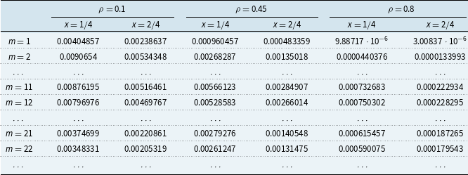


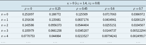

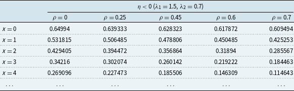


 Open access