


1. Introduction
Wall-bounded turbulence is fundamental to a wide range of engineering and natural systems, governing critical processes such as skin-friction drag, heat and mass transfer and the onset of flow instabilities. The near-wall region, including the viscous sublayer, buffer layer and lower logarithmic layer, plays a dominant role in the dynamics of wall-bounded flows, as this is where turbulent kinetic energy is both generated and dissipated at the highest rates (Townsend Reference Townsend1961; Pope Reference Pope2001). Coherent structures in these regions, such as streamwise streaks and quasi-streamwise vortices, are known to mediate the transfer of momentum and energy across scales, and their spatiotemporal organisation governs the emergence of larger-scale turbulent motions farther from the wall (Adrian Reference Adrian2007; Hwang et al. Reference Hwang, Lee, Sung and Zaki2016). Therefore, near-wall turbulence has long been the focus of flow-control strategies aimed at reducing drag, delaying transition or enhancing mixing (Kim Reference Kim2007). However, implementing such strategies in practice demands high-fidelity instantaneous flow-field information, which remains challenging due to small spatial scales, high temporal variability and limited accessibility of measurements in this region.
Wall-mounted sensors, such as those measuring pressure or wall shear stress, are relatively easy to deploy, offering time-resolved, scalable and non-disruptive access to the surface signatures of near-wall turbulence (Löfdahl & Gad-el Hak Reference Löfdahl and Gad-el Hak1999; Choi, Moin & Kim Reference Choi, Moin and Kim1994). This practical advantage has naturally led to the question of whether it is possible to reconstruct the full, off-wall velocity field using only wall-based measurements. If successful, such reconstructions would enable closed-loop control, real-time flow monitoring and improved wall models for large-eddy simulations (LES) without requiring full-field sensing. The feasibility of this task is supported by the bidirectional coupling between near-wall and outer-layer structures (Zaki Reference Zaki2024). Large-scale motions in the logarithmic and outer regions of wall-bounded flows modulate the near-wall turbulence, leaving observable imprints on wall quantities (Abe, Kawamura & Choi Reference Abe, Kawamura and Choi2004; Mathis, Hutchins & Marusic Reference Mathis, Hutchins and Marusic2009; Hwang et al. Reference Hwang, Lee, Sung and Zaki2016). Conversely, energetic near-wall events can propagate their influence outward and modulate the coherence of large-scale motions in the outer layer (Adrian Reference Adrian2007; Lozano-Durán & Jiménez Reference Lozano-Durán and Jiménez2014). These bidirectional interactions have inspired extensive efforts to infer inner velocity fields from wall measurements. Physics-based strategies often leverage data assimilation techniques to integrate wall observations into high-fidelity simulations such as direct numerical simulations (DNS) or LES, thereby reconstructing the full flow state (Colburn, Cessna & Bewley Reference Colburn, Cessna and Bewley2011; Suzuki & Hasegawa Reference Suzuki and Hasegawa2017; Wang & Zaki Reference Wang and Zaki2025). While these methods benefit from governing equations that enforce physical consistency, they remain computationally prohibitive for most practical settings. Alternatively, resolvent analysis provides a linearised, reduced-order mapping between wall forcing and flow response (Amaral et al. Reference Amaral, Cavalieri, Martini, Jordan and Towne2021). While insightful, these models rely on simplifying assumptions (e.g. linearisation around a mean flow) and cannot fully capture the nonlinear and intermittent nature of near-wall turbulence.
On the other hand, data-driven methods offer an attractive alternative for flow estimation and reconstruction, particularly in scenarios where repeated measurements are available, and the underlying physics are too complex to be modelled directly. Early work using linear stochastic estimation (LSE) (Adrian & Moin Reference Adrian and Moin1988; Marusic, Mathis & Hutchins Reference Marusic, Mathis and Hutchins2010; Baars, Hutchins & Marusic Reference Baars, Hutchins and Marusic2016; Encinar & Jiménez Reference Encinar and Jiménez2019) and proper orthogonal decomposition (Towne, Schmidt & Colonius Reference Towne, Schmidt and Colonius2018) laid the foundation by extracting statistically dominant flow features and their correlations with wall signals. These techniques, however, are constrained by their linearity, and often fail to resolve the complex, multiscale turbulence structures. With the advent of deep learning, convolutional neural networks (CNNs) and their variants have emerged as powerful tools for nonlinear flow estimation from wall data (Güemes et al. Reference Güemes, Discetti and Ianiro2019; Guastoni et al. Reference Guastoni, Güemes, Ianiro, Discetti, Schlatter, Azizpour and Vinuesa2021; Balasubramanian et al. Reference Balasubramanian, Guastoni, Schlatter, Azizpour and Vinuesa2023; Cuéllar et al. Reference Cuéllar, Güemes, Ianiro, Flores, Vinuesa and Discetti2024a ; Yousif et al. Reference Yousif, Yu, Hoyas, Vinuesa and Lim2023; Hora et al. Reference Hora, Gentine, Momen and Giometto2024). These models have demonstrated promising results in reconstructing velocity fields at various wall-normal locations using wall shear stress or pressure as input. Despite these advances, most of the existing approaches remain fundamentally deterministic and do not account for the inherent uncertainty of the reconstruction task, which arises from spatially heterogeneous correlations and variability in wall measurement quality, such as practical imperfections, induced sensor noise, limited spatial resolution and intrusive measurement effects. In regions where wall-flow coherence is strong (e.g. within the viscous sublayer), deterministic models may perform well. However, as the correlation decays with wall-normal distance, especially across the buffer and logarithmic layers (Wang, Wang & Zaki Reference Wang, Wang and Zaki2022; Arranz & Lozano-Durán Reference Arranz and Lozano-Durán2024), these models often fail to recover energetic but weakly observable flow features. Furthermore, practical limitations such as sensor sparsity, measurement noise and resolution constraints exacerbate this challenge, making the reconstruction problem increasingly ill-posed (Güemes et al. Reference Güemes, Discetti, Ianiro, Sirmacek, Azizpour and Vinuesa2021; Cuéllar et al. Reference Cuéllar, Ianiro and Discetti2024b ). As a result, deterministic models tend to produce overly smooth or biased estimates that suppress physically realistic variability. These limitations highlight the need for probabilistic modelling frameworks that not only generate physically consistent velocity features that are weakly correlated to wall quantities, but also quantify predictive uncertainty, enabling robust inference under imperfect or incomplete wall data.
Generative modelling, particularly when combined with Bayesian learning, offers a promising solution to these challenges. Rather than producing a single estimate, generative models learn the conditional distribution of turbulent velocity fields given wall measurements, enabling the synthesis of multiple physically plausible flow realisations that reflect both the informative and non-informative components of the flow with respect to wall data. Recent advances in generative AI, particularly diffusion-based models, have demonstrated impressive capabilities in synthesising high-fidelity flow realisations with accurate statistics (Rühling Cachay et al. Reference Rühling Cachay, Zhao, Joren and Yu2023; Kohl, Chen & Thuerey Reference Kohl, Chen and Thuerey2023; Li et al. Reference Li, Buzzicotti, Biferale, Bonaccorso, Chen and Wan2023; Shu, Li & Farimani Reference Shu, Li and Farimani2023; Dong, Chen & Wu Reference Dong, Chen and Wu2024; Du et al. Reference Du, Parikh, Fan, Liu and Wang2024; Gao et al. Reference Gao, Han, Fan, Sun, Liu, Duan and Wang2024a , Reference Gao, Kaltenbach and Koumoutsakosb ; Molinaro et al. Reference Molinaro2024; Fan, Akhare & Wang Reference Fan, Akhare and Wang2025; Gao, Kaltenbach & Koumoutsakos Reference Gao, Kaltenbach and Koumoutsakos2025; Shehata, Holzschuh & Thuerey Reference Shehata, Holzschuh and Thuerey2025; Zhuang, Cheng & Duraisamy Reference Zhuang, Cheng and Duraisamy2025). Specifically, Wang and co-workers have developed a conditional neural field-based latent diffusion model, which has been successfully demonstrated in generating spatiotemporal wall-bounded turbulence in three dimensions that is both inhomogeneous and anisotropic, enabling applications such as synthetic inflow turbulence generation and zero-shot spatiotemporal flow reconstruction (Du et al. Reference Du, Parikh, Fan, Liu and Wang2024; Liu et al. Reference Liu, Parikh, Fan, Du, Wang, Chen and Wang2025). However, diffusion-based sampling remains computationally expensive due to its iterative nature and is sensitive to posterior conditioning. Recently, flow matching has emerged as a scalable alternative to diffusion, offering fast and stable sampling by learning continuous-time transport maps between simple base distributions and complex data distributions through direct supervision (Lipman et al. Reference Lipman, Chen, Ben-Hamu, Nickel and Le2022).
In this work, we propose a novel generative learning framework for reconstructing near-wall turbulent velocity fields from wall-based measurements with quantified uncertainty. Specifically, we develop a conditional generative model that integrates conditional flow matching (Lipman et al. Reference Lipman, Chen, Ben-Hamu, Nickel and Le2022) with Bayesian neural operators trained using stochastic weight-averaging Gaussian (SWAG) (Maddox et al. Reference Maddox, Izmailov, Garipov, Vetrov and Wilson2019). The conditional-flow-matching-based model enables efficient generation of diverse, physically consistent instantaneous velocity fluctuation fields across multiple wall-normal locations, while the SWAG-based operator serves as a probabilistic forward model that maps velocity fields to wall measurements with quantified epistemic uncertainty. At inference time, our framework performs zero-shot conditional generation by iteratively refining sampled velocity fields to satisfy wall measurements – whether sparse, noisy or partial – without requiring re-training, transfer learning or fine-tuning.
To the best of our knowledge, this work presents the first attempt to leverage flow matching to reconstruct inhomogeneous and anisotropic turbulent velocity fluctuations at pre-defined wall-normal locations. Moreover, it is the first to demonstrate zero-shot conditional flow generation with uncertainty quantification in this context. By explicitly modelling both flow variability and predictive uncertainty, our framework addresses the ill-posed nature of near-wall turbulence reconstruction and enables robust, data-consistent inference under realistic sensing conditions. The remainder of this paper is organised as follows. Section 2 details the methodology of the proposed generative modelling framework. Section 3 presents reconstruction results under varying sensor conditions, demonstrating the effectiveness of the proposed methods. Section 4 compares the performance of the proposed model against the state-of-the-art baseline methods and discusses each individual component of the proposed framework. Finally, § 5 summarises the key findings and outlines directions for future research.
2. Methodology
2.1. Problem formulation and analysis
This study tackles the challenge of reconstructing instantaneous velocity fluctuations at various wall-normal locations using only measurements acquired at the wall. The complexity of this task varies significantly across the near-wall region due to spatially heterogeneous correlations between wall measurements (e.g. wall shear stress) and turbulent structures in wall-bounded flows. Rather than focusing on a specific off-wall plane, our goal is to develop a general-purpose generative learning framework capable of synthesising physically realistic velocity fields throughout the entire near-wall region. Critically, the proposed framework explicitly quantifies predictive uncertainty, especially in regions where the coherence between wall signals and turbulent fluctuations is weak, or where wall measurements are sparse and contaminated by noise.
To better understand the inherent challenges associated with this reconstruction task, we first analyse the correlation between wall shear stress and velocity fluctuations across different wall-normal positions. As illustrated in figures 1(a) and 1(b), the correlation strength between wall shear stress and velocity fluctuations decreases sharply as the wall-normal distance ( $y^+$
) increases. We note that this drop in correlation is slightly faster than that reported by Alfredsson et al. (Reference Alfredsson, Johansson, Haritonidis and Eckelmann1988) for two main reasons. First, our correlations are computed without incorporating any time lag, which is consistent with our entire framework. In contrast, Alfredsson et al. (Reference Alfredsson, Johansson, Haritonidis and Eckelmann1988) introduced a downstream displacement of approximately
$y^+$
) increases. We note that this drop in correlation is slightly faster than that reported by Alfredsson et al. (Reference Alfredsson, Johansson, Haritonidis and Eckelmann1988) for two main reasons. First, our correlations are computed without incorporating any time lag, which is consistent with our entire framework. In contrast, Alfredsson et al. (Reference Alfredsson, Johansson, Haritonidis and Eckelmann1988) introduced a downstream displacement of approximately $50l^*$
(where
$50l^*$
(where $l^*$
is the viscous length scale) between the wall shear stress probe and the velocity measurement, thereby accounting for the convective delay of coherent structures. Recent work by Arranz & Lozano-Durán (Reference Arranz and Lozano-Durán2024) shows that including such a lag typically increases the measured correlations. Second, the relatively low Reynolds number (
$l^*$
is the viscous length scale) between the wall shear stress probe and the velocity measurement, thereby accounting for the convective delay of coherent structures. Recent work by Arranz & Lozano-Durán (Reference Arranz and Lozano-Durán2024) shows that including such a lag typically increases the measured correlations. Second, the relatively low Reynolds number ( $\textit{Re}_\tau =180$
) considered in our study contributes to the more rapid decay. As seen in figure 1(b), at
$\textit{Re}_\tau =180$
) considered in our study contributes to the more rapid decay. As seen in figure 1(b), at $y^+=100$
, the measurement point is already near the channel centre, where the influence of wall dynamics is weak and the correlation with wall shear stress naturally approaches zero. This reduction significantly limits the feasibility of accurately reconstructing instantaneous turbulent structures in outer regions using solely wall-based measurements (Suzuki & Hasegawa Reference Suzuki and Hasegawa2017; Wang et al. Reference Wang, Wang and Zaki2022). Nonetheless, large-scale flow structures in the outer region leave subtle yet detectable imprints on the wall through amplitude and wavelength modulation effects, indirectly encoding useful information within wall shear stress fluctuations (Arranz & Lozano-Durán Reference Arranz and Lozano-Durán2024; Mathis et al. Reference Mathis, Hutchins and Marusic2009). Recognising this indirect yet informative coupling motivates our generative model, which aims to reconstruct instantaneous velocity fluctuations at various off-wall locations, incorporating uncertainty quantification that reflects the progressive weakening of coherence, measurement sparsity and observational noise.
$y^+=100$
, the measurement point is already near the channel centre, where the influence of wall dynamics is weak and the correlation with wall shear stress naturally approaches zero. This reduction significantly limits the feasibility of accurately reconstructing instantaneous turbulent structures in outer regions using solely wall-based measurements (Suzuki & Hasegawa Reference Suzuki and Hasegawa2017; Wang et al. Reference Wang, Wang and Zaki2022). Nonetheless, large-scale flow structures in the outer region leave subtle yet detectable imprints on the wall through amplitude and wavelength modulation effects, indirectly encoding useful information within wall shear stress fluctuations (Arranz & Lozano-Durán Reference Arranz and Lozano-Durán2024; Mathis et al. Reference Mathis, Hutchins and Marusic2009). Recognising this indirect yet informative coupling motivates our generative model, which aims to reconstruct instantaneous velocity fluctuations at various off-wall locations, incorporating uncertainty quantification that reflects the progressive weakening of coherence, measurement sparsity and observational noise.

Figure 1. (a) Instantaneous streamwise velocity fluctuations $\boldsymbol{u}'$
of the turbulent channel flow (
$\boldsymbol{u}'$
of the turbulent channel flow ( $\textit{Re}_\tau = 180$
) at three wall-normal locations (
$\textit{Re}_\tau = 180$
) at three wall-normal locations ( $y^+ = 5, 20, 40$
) alongside the corresponding wall shear stress field
$y^+ = 5, 20, 40$
) alongside the corresponding wall shear stress field $\tau _{u}$
. (b) Correlation coefficients
$\tau _{u}$
. (b) Correlation coefficients $C_{\tau _u, {u}'}$
between wall shear stress and velocity fluctuations as a function of
$C_{\tau _u, {u}'}$
between wall shear stress and velocity fluctuations as a function of $y^+$
. (c) Reconstruction concept: given wall input
$y^+$
. (c) Reconstruction concept: given wall input ${\boldsymbol{\varPhi }}_{w\textit{all}}$
, the model (parametrised by
${\boldsymbol{\varPhi }}_{w\textit{all}}$
, the model (parametrised by $\boldsymbol{\theta }$
) predicts
$\boldsymbol{\theta }$
) predicts $\boldsymbol{u}'$
at different off-wall planes, with increasing uncertainty illustrated by blurred regions at higher
$\boldsymbol{u}'$
at different off-wall planes, with increasing uncertainty illustrated by blurred regions at higher $y^+$
.
$y^+$
.
Specifically, within the viscous sublayer, velocity fluctuations exhibit a nearly linear and direct relationship with wall measurements, characterised by a high correlation coefficient ( $C_{\tau _{u} u'} \approx 1$
) (Wang et al. Reference Wang, Wang and Zaki2022). Due to this strong coupling, velocity fields in this region can be reconstructed accurately with minimal uncertainty, as illustrated conceptually in figure 1(c). Moving outward into the buffer layer, however, this direct coherence rapidly decays (Wang et al. Reference Wang, Wang and Zaki2022), even though this region is critical for turbulent kinetic energy production and hosts energetic coherent structures, such as streamwise streaks and hairpin vortices (Adrian Reference Adrian2007; Bae & Lee Reference Bae and Lee2021). These dynamically important structures are only indirectly captured by wall signals due to modulation effects, significantly complicating their instantaneous reconstruction. Thus, while the deterministic models can perform well in terms of mean prediction accuracy, they cannot capture the variability and provide predictive uncertainty that are particularly important in the buffer layer. This limitation underscores the need for probabilistic modelling approaches that explicitly quantify the uncertainty arising from weakened correlations and indirect observability. Further away from the wall (logarithmic layer and beyond), large-scale turbulent motions, particularly low-speed streaks, persist and can extend significantly into the outer layer, sometimes reaching the boundary-layer edge (Adrian Reference Adrian2007; Encinar & Jiménez Reference Encinar and Jiménez2019). Although their instantaneous correlation with wall signals is generally low, these large-scale structures indirectly influence near-wall dynamics through modulation effects, leaving distinguishable but indirect signatures on wall quantities (Arranz & Lozano-Durán Reference Arranz and Lozano-Durán2024; Mathis et al. Reference Mathis, Hutchins and Marusic2009). Despite being less dominant energetically compared with smaller-scale structures nearer to the wall, accurately capturing their statistical features remains essential to realistically reconstruct turbulence characteristics. Deterministic methods relying solely on wall measurements often significantly underestimate fluctuations in this region, as they only recover weakly correlated, low-energy large-scale motions (Guastoni et al. Reference Guastoni, Güemes, Ianiro, Discetti, Schlatter, Azizpour and Vinuesa2021). Recognising this limitation, our framework not only predicts informative components directly from wall data, but also leverages generative learning to synthesise non-informative yet energetically crucial turbulence structures, thereby ensuring accurate statistical reconstructions.
$C_{\tau _{u} u'} \approx 1$
) (Wang et al. Reference Wang, Wang and Zaki2022). Due to this strong coupling, velocity fields in this region can be reconstructed accurately with minimal uncertainty, as illustrated conceptually in figure 1(c). Moving outward into the buffer layer, however, this direct coherence rapidly decays (Wang et al. Reference Wang, Wang and Zaki2022), even though this region is critical for turbulent kinetic energy production and hosts energetic coherent structures, such as streamwise streaks and hairpin vortices (Adrian Reference Adrian2007; Bae & Lee Reference Bae and Lee2021). These dynamically important structures are only indirectly captured by wall signals due to modulation effects, significantly complicating their instantaneous reconstruction. Thus, while the deterministic models can perform well in terms of mean prediction accuracy, they cannot capture the variability and provide predictive uncertainty that are particularly important in the buffer layer. This limitation underscores the need for probabilistic modelling approaches that explicitly quantify the uncertainty arising from weakened correlations and indirect observability. Further away from the wall (logarithmic layer and beyond), large-scale turbulent motions, particularly low-speed streaks, persist and can extend significantly into the outer layer, sometimes reaching the boundary-layer edge (Adrian Reference Adrian2007; Encinar & Jiménez Reference Encinar and Jiménez2019). Although their instantaneous correlation with wall signals is generally low, these large-scale structures indirectly influence near-wall dynamics through modulation effects, leaving distinguishable but indirect signatures on wall quantities (Arranz & Lozano-Durán Reference Arranz and Lozano-Durán2024; Mathis et al. Reference Mathis, Hutchins and Marusic2009). Despite being less dominant energetically compared with smaller-scale structures nearer to the wall, accurately capturing their statistical features remains essential to realistically reconstruct turbulence characteristics. Deterministic methods relying solely on wall measurements often significantly underestimate fluctuations in this region, as they only recover weakly correlated, low-energy large-scale motions (Guastoni et al. Reference Guastoni, Güemes, Ianiro, Discetti, Schlatter, Azizpour and Vinuesa2021). Recognising this limitation, our framework not only predicts informative components directly from wall data, but also leverages generative learning to synthesise non-informative yet energetically crucial turbulence structures, thereby ensuring accurate statistical reconstructions.

Figure 2. (a) Flow-matching-based generative model $\boldsymbol{\nu }_{\boldsymbol{\theta }}$
for synthesising novel instances of velocity fluctuations
$\boldsymbol{\nu }_{\boldsymbol{\theta }}$
for synthesising novel instances of velocity fluctuations $(u',\ v',\ w')$
. (b) Forward operator with SWAG
$(u',\ v',\ w')$
. (b) Forward operator with SWAG $\mathcal{F}_{\boldsymbol{\phi }}$
to quantify the epistemic uncertainty between velocity fluctuations
$\mathcal{F}_{\boldsymbol{\phi }}$
to quantify the epistemic uncertainty between velocity fluctuations $(u',\ v',\ w')$
and wall quantities
$(u',\ v',\ w')$
and wall quantities $(p',\ \tau _u,\ \tau _w)$
. (c) Training-free conditional generation based on the predictor–corrector FM inference algorithm using conditional information
$(p',\ \tau _u,\ \tau _w)$
. (c) Training-free conditional generation based on the predictor–corrector FM inference algorithm using conditional information $\boldsymbol{y}$
.
$\boldsymbol{y}$
.
2.2. Overview of proposed generative modelling framework for near-wall turbulence
Building upon our analysis of spatially heterogeneous correlations between wall measurements and turbulent structures, we propose a generative modelling framework explicitly designed to reconstruct instantaneous velocity fluctuations across multiple wall-normal locations. Specifically, a representative wall-normal location from each of the viscous sublayer, buffer and logarithmic layers is chosen to systematically evaluate the data assimilation and uncertainty quantification capabilities of the proposed generative framework. The comprehensiveness of this test stems from assessing the framework’s performance in three distinct regimes based on the classification introduced in Arranz & Lozano-Durán (Reference Arranz and Lozano-Durán2024): the highly informative viscous sublayer ( $y^+=5$
), the partially informative buffer layer (
$y^+=5$
), the partially informative buffer layer ( $y^+=20$
) and the almost non-informative logarithmic layer (
$y^+=20$
) and the almost non-informative logarithmic layer ( $y^+=40$
). This approach provides a thorough analysis of the proposed framework across different operating conditions. The core idea of the framework leverages generative learning combined with probabilistic neural operators within a Bayesian framework to effectively handle the inherent uncertainties and indirect observability in wall-bounded turbulence. Figure 2 illustrates the three key components of our framework.
$y^+=40$
). This approach provides a thorough analysis of the proposed framework across different operating conditions. The core idea of the framework leverages generative learning combined with probabilistic neural operators within a Bayesian framework to effectively handle the inherent uncertainties and indirect observability in wall-bounded turbulence. Figure 2 illustrates the three key components of our framework.
In the training phase (figure 2
a), a generative model based on flow matching (Lipman et al. Reference Lipman, Chen, Ben-Hamu, Nickel and Le2022) is built to generate instantaneous full-field velocity fluctuation samples at pre-defined wall-normal positions ( $y^+ = 5, 20, 40$
) by sampling from a standard Gaussian distribution,
$y^+ = 5, 20, 40$
) by sampling from a standard Gaussian distribution, $\mathcal{N}(\boldsymbol{0}, \boldsymbol{I})$
. The trained model is able to randomly synthesise novel, physically plausible instantaneous velocity fluctuation fields consistent with the statistical features observed in turbulent channel flows. The details of the flow-matching training are further elaborated in § 2.3. Concurrently, as depicted in figure 2(b), a probabilistic neural operator is designed to predict wall quantities (e.g. wall shear stresses and pressures) from the velocity fluctuations with quantified uncertainties. This U-Net-based neural operator is trained probabilistically using SWAG (Maddox et al. Reference Maddox, Izmailov, Garipov, Vetrov and Wilson2019), a Bayesian learning technique enabling the quantification of epistemic uncertainty inherent in neural network predictions. The incorporation of the SWAG operator is critical as it allows our framework to explicitly learn the uncertainty arising from weak correlations, measurement sparsity and noise. As the generative model and the SWAG neural operator utilised in this work are based on CNNs, the current formulation requires access to the entire field of velocity fluctuations and wall measurements on a uniform grid during the training process.
$\mathcal{N}(\boldsymbol{0}, \boldsymbol{I})$
. The trained model is able to randomly synthesise novel, physically plausible instantaneous velocity fluctuation fields consistent with the statistical features observed in turbulent channel flows. The details of the flow-matching training are further elaborated in § 2.3. Concurrently, as depicted in figure 2(b), a probabilistic neural operator is designed to predict wall quantities (e.g. wall shear stresses and pressures) from the velocity fluctuations with quantified uncertainties. This U-Net-based neural operator is trained probabilistically using SWAG (Maddox et al. Reference Maddox, Izmailov, Garipov, Vetrov and Wilson2019), a Bayesian learning technique enabling the quantification of epistemic uncertainty inherent in neural network predictions. The incorporation of the SWAG operator is critical as it allows our framework to explicitly learn the uncertainty arising from weak correlations, measurement sparsity and noise. As the generative model and the SWAG neural operator utilised in this work are based on CNNs, the current formulation requires access to the entire field of velocity fluctuations and wall measurements on a uniform grid during the training process.
In the inference stage, depicted in figure 2(c), our framework is able to perform conditional generation in a zero-shot manner (i.e. without re-training) using a predictor–corrector sampling approach. Specifically, given instantaneous wall measurements, the pre-trained generative model synthesises instantaneous velocity fluctuation fields that are consistent with these sensor data. This is accomplished through iterative refinement, where an initial prediction from the generative model is progressively updated using gradient-based corrections derived from discrepancies between predicted and actual wall data. The gradients are computed via the differentiable forward measurement model integrated with the probabilistic SWAG operator, thereby ensuring that the synthesised velocity fluctuations realistically reflect measurement uncertainties and the physical constraints imposed by available wall information. Further details are provided in § 2.4.
In summary, our proposed generative modelling framework uniquely integrates generative learning and scalable uncertainty quantification techniques, providing robust and physically consistent reconstructions of turbulent velocity fluctuations from limited wall-based measurements.
2.3. Flow matching for generative modelling of instantaneous velocity fluctuations
To model the complex, high-dimensional distribution of instantaneous velocity fluctuations in near-wall turbulence, we adopt the recently proposed flow matching (FM) framework (Lipman et al. Reference Lipman, Chen, Ben-Hamu, Nickel and Le2022), which enables tractable and scalable training of continuous normalising flows by directly learning the velocity fields that transport probability mass from a simple base distribution to the target data distribution. Unlike conventional continuous normalising flows, which require density estimation via the change-of-variables formula and involve solving ordinary differential equations (ODEs) during training, FM bypasses these limitations by re-framing the generative modelling as a regression task over velocity fields that define transport paths between distributions. This makes FM particularly suitable for large-scale, high-dimensional turbulent flow data. In this work, we present the first use of FM to generate inhomogeneous, anisotropic turbulence by reconstructing the three velocity fluctuation components at the chosen wall-normal positions ( $y^+ = 5, 20, 40$
).
$y^+ = 5, 20, 40$
).
Let $\boldsymbol{x}_1 \sim P_1(\boldsymbol{x})$
denote a sample drawn from the target data distribution, where each sample represents a snapshot of the instantaneous three-component velocity fluctuation field at a specified wall-normal location
$\boldsymbol{x}_1 \sim P_1(\boldsymbol{x})$
denote a sample drawn from the target data distribution, where each sample represents a snapshot of the instantaneous three-component velocity fluctuation field at a specified wall-normal location $y^+$
. Specifically,
$y^+$
. Specifically, $\boldsymbol{x}_1 = [u'(x, z, t), v'(x, z, t), w'(x, z, t)]$
are defined on a discrete
$\boldsymbol{x}_1 = [u'(x, z, t), v'(x, z, t), w'(x, z, t)]$
are defined on a discrete $(x, z)$
grid, where
$(x, z)$
grid, where $x, z$
are wall-parallel coordinates and
$x, z$
are wall-parallel coordinates and $t$
denotes physical time. We define the base distribution
$t$
denotes physical time. We define the base distribution $P_0(\boldsymbol{x}) = \mathcal{N}(\boldsymbol{0}, \boldsymbol{I})$
as a standard multivariate Gaussian in the same space as the target data. Our goal is to learn a transport neural velocity field
$P_0(\boldsymbol{x}) = \mathcal{N}(\boldsymbol{0}, \boldsymbol{I})$
as a standard multivariate Gaussian in the same space as the target data. Our goal is to learn a transport neural velocity field $\boldsymbol{\nu }_{\boldsymbol{\theta }}(\tau , \boldsymbol{x}_\tau )$
, parametrised by neural network weights
$\boldsymbol{\nu }_{\boldsymbol{\theta }}(\tau , \boldsymbol{x}_\tau )$
, parametrised by neural network weights $\boldsymbol{\theta }$
, that smoothly transforms samples from
$\boldsymbol{\theta }$
, that smoothly transforms samples from $P_0$
into samples from
$P_0$
into samples from $P_1$
along a continuous path indexed by a fictitious time variable
$P_1$
along a continuous path indexed by a fictitious time variable $\tau \in [0, 1]$
. The generative process is defined by the flow ODE
$\tau \in [0, 1]$
. The generative process is defined by the flow ODE
 \begin{equation} \frac {{\rm d}\boldsymbol{x}_\tau }{{\rm d}\tau } = \boldsymbol{\nu }_{\boldsymbol{\theta }}(\tau , \boldsymbol{x}_\tau ), \end{equation}
where $\boldsymbol{x}_\tau$
denotes the sample at intermediate time
$\boldsymbol{x}_\tau$
denotes the sample at intermediate time $\tau$
along the transport trajectory from
$\tau$
along the transport trajectory from $P_0$
to
$P_0$
to $P_1$
.
$P_1$
.
To ensure probability conservation along the flow, the transport velocity field $\boldsymbol{\nu }(\tau , \boldsymbol{x}_\tau )$
must satisfy the continuity equation
$\boldsymbol{\nu }(\tau , \boldsymbol{x}_\tau )$
must satisfy the continuity equation
 \begin{equation} \frac {\partial\! P_\tau }{\partial \tau } = - \boldsymbol{\nabla }\boldsymbol{\cdot }(P_\tau \boldsymbol{\nu }_\tau ), \end{equation}
where $P_\tau (\boldsymbol{x})$
denotes the intermediate distribution at time
$P_\tau (\boldsymbol{x})$
denotes the intermediate distribution at time $\tau$
. If the true velocity field
$\tau$
. If the true velocity field $\boldsymbol{\nu }(\tau , \boldsymbol{x}_\tau )$
is known, we can directly minimise the following loss:
$\boldsymbol{\nu }(\tau , \boldsymbol{x}_\tau )$
is known, we can directly minimise the following loss:
 \begin{equation} \mathcal{L}(\boldsymbol{\theta }) := \mathbb{E}_{\tau \sim {U}[0,1], \boldsymbol{x}_\tau \sim P_\tau (\boldsymbol{x}_\tau )}\big \|\boldsymbol{\nu }_{\boldsymbol{\theta }}(\tau , \boldsymbol{x}_\tau ) - \boldsymbol{\nu }(\tau , \boldsymbol{x}_\tau )\big \|^2. \end{equation}
In practice, however, directly evaluating the true velocity $\boldsymbol{\nu }(\tau , \boldsymbol{x}_\tau )$
and sampling from
$\boldsymbol{\nu }(\tau , \boldsymbol{x}_\tau )$
and sampling from $P_\tau (\boldsymbol{x}_\tau )$
is intractable. To address this, FM introduces a conditional formulation by introducing a latent variable
$P_\tau (\boldsymbol{x}_\tau )$
is intractable. To address this, FM introduces a conditional formulation by introducing a latent variable $\boldsymbol{z} \sim q(\boldsymbol{z})$
that leads to conditional intermediate distributions
$\boldsymbol{z} \sim q(\boldsymbol{z})$
that leads to conditional intermediate distributions $P_\tau (\boldsymbol{x}|\boldsymbol{z})$
and velocities
$P_\tau (\boldsymbol{x}|\boldsymbol{z})$
and velocities $\boldsymbol{\nu }(\boldsymbol{x}_\tau |\boldsymbol{z})$
, such that
$\boldsymbol{\nu }(\boldsymbol{x}_\tau |\boldsymbol{z})$
, such that
 \begin{align} P_\tau (\boldsymbol{x}_\tau ) &= \int P_\tau (\boldsymbol{x}_\tau |\boldsymbol{z})q(\boldsymbol{z}){\rm d}\boldsymbol{z}, \end{align}
 \begin{align} \boldsymbol{\nu }_\tau (\tau ,\boldsymbol{x}_\tau ) &= \int \frac {\boldsymbol{\nu }_\tau (\boldsymbol{x}_\tau |\boldsymbol{z}) P_\tau (\boldsymbol{x}_\tau |\boldsymbol{z})}{P_\tau (\boldsymbol{x}_\tau )}q(\boldsymbol{z}){\rm d}\boldsymbol{z} = \mathbb{E}_{q(\boldsymbol{z})}\bigg [ \frac {\boldsymbol{\nu }_\tau (\boldsymbol{x}_\tau |\boldsymbol{z}) P_\tau (\boldsymbol{x}_\tau |\boldsymbol{z})}{P_t(\boldsymbol{x}_\tau )}\bigg ]. \end{align}
Substituting (2.3) into the FM loss and swapping the gradient and expectation under suitable regularity conditions leads to the modified loss:
 \begin{equation} \tilde {\mathcal{L}}(\boldsymbol{\theta }) = \mathbb{E}_{\tau \sim \mathcal{U}[0,1], \boldsymbol{z} \sim q(\boldsymbol{z}), \boldsymbol{x}_\tau \sim P_\tau (\boldsymbol{x} | \boldsymbol{z})} \big \| \boldsymbol{\nu }_{\boldsymbol{\theta }}(\tau , \boldsymbol{x}_\tau ) - \boldsymbol{\nu }(\tau , \boldsymbol{x}_\tau | \boldsymbol{z}) \big \|^2. \end{equation}
Under certain assumptions on $q(\boldsymbol{z})$
and
$q(\boldsymbol{z})$
and $P_\tau (\boldsymbol{x}_\tau |\boldsymbol{z})$
(Lipman et al. Reference Lipman, Chen, Ben-Hamu, Nickel and Le2022), it can be proved that the gradient of the modified loss yields the same optimisation objective as the original FM loss, i.e.
$P_\tau (\boldsymbol{x}_\tau |\boldsymbol{z})$
(Lipman et al. Reference Lipman, Chen, Ben-Hamu, Nickel and Le2022), it can be proved that the gradient of the modified loss yields the same optimisation objective as the original FM loss, i.e.
 \begin{equation} \boldsymbol{\nabla} _{\boldsymbol{\theta }} \mathcal{L}(\boldsymbol{\theta }) = \boldsymbol{\nabla} _{\boldsymbol{\theta }} \tilde {\mathcal{L}}(\boldsymbol{\theta }). \end{equation}
Therefore, the neural velocity field can be trained based on the conditional formulation of the loss function, where both the conditional intermediate distributions and velocities are available. In practice, we use empirical samples from the data distribution as conditioning variables. Specifically, we let $q(\boldsymbol{z}) = (1/N) \sum _{i=1}^{N} \delta (\boldsymbol{z} - \boldsymbol{x}_1^{(i)})$
, where
$q(\boldsymbol{z}) = (1/N) \sum _{i=1}^{N} \delta (\boldsymbol{z} - \boldsymbol{x}_1^{(i)})$
, where $\{\boldsymbol{x}_1^{(i)}\}_{i=1}^N$
are training velocity fluctuation data. Then we have the following tractable definitions for the conditional intermediate distribution and velocity:
$\{\boldsymbol{x}_1^{(i)}\}_{i=1}^N$
are training velocity fluctuation data. Then we have the following tractable definitions for the conditional intermediate distribution and velocity:
 \begin{align} P_\tau (\boldsymbol{x}_\tau | \boldsymbol{x}_1) &= \mathcal{N}\big (\tau \boldsymbol{x}_1, \big [1 - (1 - \sigma _{\textit{min}})\tau \big ]^2\boldsymbol{I}\big ), \end{align}
 \begin{align} \boldsymbol{\nu }(\tau , \boldsymbol{x}_\tau | \boldsymbol{x}_1) &= \frac {\boldsymbol{x}_1 - (1 - \sigma _{\textit{min}})\boldsymbol{x}_\tau }{1 - (1 - \sigma _{\textit{min}})\tau }, \end{align}
which corresponds to an isotropic Gaussian interpolation with linearly evolving mean and covariance from $\mathcal{N}(0, \boldsymbol{I})$
to
$\mathcal{N}(0, \boldsymbol{I})$
to $\mathcal{N}(\boldsymbol{x}_1, \sigma _{\textit{min}}^2 \boldsymbol{I})$
. Here, the mean interpolates linearly from
$\mathcal{N}(\boldsymbol{x}_1, \sigma _{\textit{min}}^2 \boldsymbol{I})$
. Here, the mean interpolates linearly from $\boldsymbol{0}$
to
$\boldsymbol{0}$
to $\boldsymbol{x}_1$
, while the covariance linearly decays from
$\boldsymbol{x}_1$
, while the covariance linearly decays from $\boldsymbol{I}$
to
$\boldsymbol{I}$
to $\sigma _{\textit{min}}^2 \boldsymbol{I}$
. This results in a simple and tractable sampling scheme, where both the intermediate samples
$\sigma _{\textit{min}}^2 \boldsymbol{I}$
. This results in a simple and tractable sampling scheme, where both the intermediate samples $\boldsymbol{x}_\tau$
and their associated transport velocities
$\boldsymbol{x}_\tau$
and their associated transport velocities $\boldsymbol{\nu }(\tau , \boldsymbol{x}_\tau | \boldsymbol{x}_1)$
are available in closed form for supervised training. Additionally, the neural velocity field
$\boldsymbol{\nu }(\tau , \boldsymbol{x}_\tau | \boldsymbol{x}_1)$
are available in closed form for supervised training. Additionally, the neural velocity field $\boldsymbol{\nu }_{\boldsymbol{\theta }}(\tau , \boldsymbol{x}_\tau )$
is trained in a class-conditional way for the different wall-normal distances of
$\boldsymbol{\nu }_{\boldsymbol{\theta }}(\tau , \boldsymbol{x}_\tau )$
is trained in a class-conditional way for the different wall-normal distances of $y^+=\{5,\, 20,\, 40\}$
considered in this study. The model learns a trainable neural embedding corresponding to each wall-normal distance. The details of network architectures are provided in Appendix A.
$y^+=\{5,\, 20,\, 40\}$
considered in this study. The model learns a trainable neural embedding corresponding to each wall-normal distance. The details of network architectures are provided in Appendix A.
Once the FM model $\boldsymbol{\nu }_{\boldsymbol{\theta }}$
is trained, novel samples of the velocity fluctuations are generated by sampling from
$\boldsymbol{\nu }_{\boldsymbol{\theta }}$
is trained, novel samples of the velocity fluctuations are generated by sampling from $P_0(\boldsymbol{x}_0)$
and solving the ODE in (2.1) by integrating
$P_0(\boldsymbol{x}_0)$
and solving the ODE in (2.1) by integrating $\boldsymbol{\nu }_{\boldsymbol{\theta }}(\tau , \boldsymbol{x}_\tau )$
over the fictitious time interval
$\boldsymbol{\nu }_{\boldsymbol{\theta }}(\tau , \boldsymbol{x}_\tau )$
over the fictitious time interval $\tau \in [0,1]$
. In this work, we employ a forward Euler scheme, and discretise the fictitious time domain into
$\tau \in [0,1]$
. In this work, we employ a forward Euler scheme, and discretise the fictitious time domain into $250$
uniform steps.
$250$
uniform steps.
2.4. Training-free conditional generation guided by wall measurements
The generative model described in § 2.3 enables efficient sampling of instantaneous velocity fluctuation fields from the learned distribution at specified wall-normal locations. While this unconditional generation captures the statistical structure of turbulent fluctuations, it does not incorporate any instance-specific observations. In practical settings, however, partial information about a specific turbulent flow realisation is often available, either in the form of direct but sparse velocity measurements within the domain or, more commonly, through indirect wall-based observations such as wall shear stress or pressure signals. These measurements $\boldsymbol{y}$
encode valuable information about the underlying flow state and can be leveraged during inference. This motivates the need for conditional generative inference that can synthesise velocity fields consistent with available observations, while retaining uncertainty quantification over unobserved regions.
$\boldsymbol{y}$
encode valuable information about the underlying flow state and can be leveraged during inference. This motivates the need for conditional generative inference that can synthesise velocity fields consistent with available observations, while retaining uncertainty quantification over unobserved regions.
A common strategy to condition generative models is to incorporate the observation vector $\boldsymbol{y}$
, whether wall measurements, sparse velocity probes, or both, into the sampling process. This is typically achieved by modifying the training objective to explicitly encode
$\boldsymbol{y}$
, whether wall measurements, sparse velocity probes, or both, into the sampling process. This is typically achieved by modifying the training objective to explicitly encode $\boldsymbol{y}$
as input, for example through input concatenation, modulation via feature-wise affine transformations, or injection via a hypernetwork
$\boldsymbol{y}$
as input, for example through input concatenation, modulation via feature-wise affine transformations, or injection via a hypernetwork $F_\phi (\boldsymbol{y})$
(Dhariwal & Nichol Reference Dhariwal and Nichol2021; Fu et al. Reference Fu, Yang, Wang and Chen2024; Jacobsen, Zhuang & Duraisamy Reference Jacobsen, Zhuang and Duraisamy2025; Zhuang et al. Reference Zhuang, Cheng and Duraisamy2025). However, these approaches require re-training the generative model for each new type of conditioning input and often scale poorly when the structure, modality or spatial extent of
$F_\phi (\boldsymbol{y})$
(Dhariwal & Nichol Reference Dhariwal and Nichol2021; Fu et al. Reference Fu, Yang, Wang and Chen2024; Jacobsen, Zhuang & Duraisamy Reference Jacobsen, Zhuang and Duraisamy2025; Zhuang et al. Reference Zhuang, Cheng and Duraisamy2025). However, these approaches require re-training the generative model for each new type of conditioning input and often scale poorly when the structure, modality or spatial extent of $\boldsymbol{y}$
varies across instances, as is the case in sensor-limited turbulence set-ups.
$\boldsymbol{y}$
varies across instances, as is the case in sensor-limited turbulence set-ups.
To overcome these limitations, we introduce a training-free conditional inference strategy that augments the unconditional FM model with a correction term derived from the conditioning measurements. Inspired by training-free conditional methods in diffusion models such as diffusion posterior sampling (Chung et al. Reference Chung, Kim, Mccann, Klasky and Ye2022; Du et al. Reference Du, Parikh, Fan, Liu and Wang2024) and Bayesian classifier guidance (Dhariwal & Nichol Reference Dhariwal and Nichol2021; Gao et al. Reference Gao, Han, Fan, Sun, Liu, Duan and Wang2024a
), our approach adapts these ideas to the FM paradigm. Specifically, we define a guided sampling procedure in which the learned transport velocity $\boldsymbol{\nu }_{\boldsymbol{\theta }}(\tau , \boldsymbol{x}_\tau )$
is augmented during inference by a correction term
$\boldsymbol{\nu }_{\boldsymbol{\theta }}(\tau , \boldsymbol{x}_\tau )$
is augmented during inference by a correction term $\boldsymbol{\nu }'(\tau , \boldsymbol{x}_\tau , \boldsymbol{y})$
that nudges the generative trajectory towards compatibility with the measurements:
$\boldsymbol{\nu }'(\tau , \boldsymbol{x}_\tau , \boldsymbol{y})$
that nudges the generative trajectory towards compatibility with the measurements:
 \begin{equation} \frac {{\rm d}\boldsymbol{x}}{{\rm d}\tau } = \boldsymbol{\nu }_{\boldsymbol{\theta }}(\tau , \boldsymbol{x}_\tau ) + \boldsymbol{\nu }'(\tau , \boldsymbol{x}_\tau , \boldsymbol{y}). \end{equation}
To derive this correction term, we first assess the discrepancy between the observations $\boldsymbol{y}$
and the predicted measurements
$\boldsymbol{y}$
and the predicted measurements $\hat {\boldsymbol{y}}$
derived from the current state
$\hat {\boldsymbol{y}}$
derived from the current state $\boldsymbol{x}_\tau$
, and then propagate this discrepancy back to
$\boldsymbol{x}_\tau$
, and then propagate this discrepancy back to $\boldsymbol{x}_\tau$
. This process involves three components: (i) an efficient approximation of the terminal state
$\boldsymbol{x}_\tau$
. This process involves three components: (i) an efficient approximation of the terminal state $\hat {\boldsymbol{x}}_1$
from intermediate states
$\hat {\boldsymbol{x}}_1$
from intermediate states $\boldsymbol{x}_\tau$
, (ii) a forward state-to-observable operator that maps the generated state to measurement space and (iii) a differentiable loss to quantify mismatch between predicted and observed measurements. In the first step, the target guidance field (2.7
b) defines a straight interpolation in data space between the noise sample and the data sample. Accordingly, we employ a one-step linear approximation of the terminal state (Lipman et al. Reference Lipman, Chen, Ben-Hamu, Nickel and Le2022):
$\boldsymbol{x}_\tau$
, (ii) a forward state-to-observable operator that maps the generated state to measurement space and (iii) a differentiable loss to quantify mismatch between predicted and observed measurements. In the first step, the target guidance field (2.7
b) defines a straight interpolation in data space between the noise sample and the data sample. Accordingly, we employ a one-step linear approximation of the terminal state (Lipman et al. Reference Lipman, Chen, Ben-Hamu, Nickel and Le2022):
 \begin{equation} \hat {\boldsymbol{x}}_{1|\tau } = \boldsymbol{x}_\tau + (1-\tau )\boldsymbol{\nu }_{\boldsymbol{\theta }}(\tau , \boldsymbol{x}_\tau ), \end{equation}
which estimates the endpoint of the flow by extrapolating along the learned transport velocity. This is computationally efficient and justified by the nearly linear nature of the flow trajectory learned through conditional flow matching (§ 2.3). Next, we define the forward operator $\mathcal{F}$
that maps the predicted state
$\mathcal{F}$
that maps the predicted state $\hat {\boldsymbol{x}}_{1|\tau }$
to the observable domain. Depending on the context,
$\hat {\boldsymbol{x}}_{1|\tau }$
to the observable domain. Depending on the context, $\mathcal{F}$
may represent a fixed linear mapping (e.g. extracting velocity values at sensor locations) or a learned neural operator that maps the off-wall flow states to indirect measurements (e.g. wall measurements). Considering measurement noises
$\mathcal{F}$
may represent a fixed linear mapping (e.g. extracting velocity values at sensor locations) or a learned neural operator that maps the off-wall flow states to indirect measurements (e.g. wall measurements). Considering measurement noises $\boldsymbol{\epsilon }$
, this operator is defined as
$\boldsymbol{\epsilon }$
, this operator is defined as
 \begin{align} \hat {\boldsymbol{y}} &= \mathcal{F}(\hat {\boldsymbol{x}}_{1|\tau }) + \boldsymbol{\epsilon }; \quad \boldsymbol{\epsilon } \sim \mathcal{N}(0, \varSigma _e) ,\end{align}
where $\varSigma _e = \sigma _e^2 \boldsymbol{I}$
captures the assumed level of aleatoric uncertainty. The aleatoric uncertainty is assumed to be a Gaussian distribution to model the measurement error of the sensors that commonly arises from the thermal or electronic noise.
$\varSigma _e = \sigma _e^2 \boldsymbol{I}$
captures the assumed level of aleatoric uncertainty. The aleatoric uncertainty is assumed to be a Gaussian distribution to model the measurement error of the sensors that commonly arises from the thermal or electronic noise.
The discrepancy $\mathscr{D}(\hat {\boldsymbol{y}}, \boldsymbol{y})$
between predicted and observed measurements is quantified via a loss function, typically the mean squared error. This loss is then differentiated with respect to
$\mathscr{D}(\hat {\boldsymbol{y}}, \boldsymbol{y})$
between predicted and observed measurements is quantified via a loss function, typically the mean squared error. This loss is then differentiated with respect to $\boldsymbol{x}_\tau$
, yielding a gradient that points in the direction of greater alignment between the generated sample and the observations. We define the correction term as
$\boldsymbol{x}_\tau$
, yielding a gradient that points in the direction of greater alignment between the generated sample and the observations. We define the correction term as
 \begin{equation} \boldsymbol{\nu }'(\tau , \boldsymbol{x}_\tau , \boldsymbol{y}) = -b ||\boldsymbol{\nu }_{\boldsymbol{\theta }}(\tau , \boldsymbol{x}_\tau )|| \frac {\boldsymbol{\nabla} _{\boldsymbol{x}_\tau } \mathscr{D}(\hat {\boldsymbol{y}}, \boldsymbol{y})}{||\boldsymbol{\nabla} _{\boldsymbol{x}_\tau } \mathscr{D}(\hat {\boldsymbol{y}}, \boldsymbol{y})||}, \end{equation}
where $b$
is a scalar that controls the guidance strength, and is set to
$b$
is a scalar that controls the guidance strength, and is set to $1$
for all the experiments considered in this study. The correction direction is aligned with the normalised loss gradient, while the magnitude is scaled to match the norm of the current transport velocity, ensuring that the guidance term and learned flow are balanced in strength.
$1$
for all the experiments considered in this study. The correction direction is aligned with the normalised loss gradient, while the magnitude is scaled to match the norm of the current transport velocity, ensuring that the guidance term and learned flow are balanced in strength.
Importantly, this conditional sampling strategy is agnostic to the nature and modality of the measurement vector $\boldsymbol{y}$
. While in this paper we focus on wall-based observations, the framework can also accommodate sparse velocity probes, inpainting of partially known flow fields or any other differentiable observation models. In fact, the proposed corrector can be viewed as a variational approximation to the gradient of the log-posterior distribution
$\boldsymbol{y}$
. While in this paper we focus on wall-based observations, the framework can also accommodate sparse velocity probes, inpainting of partially known flow fields or any other differentiable observation models. In fact, the proposed corrector can be viewed as a variational approximation to the gradient of the log-posterior distribution $\boldsymbol{\nabla} _{\boldsymbol{x}} \log P(\boldsymbol{y} | \boldsymbol{x})$
, and thus relates conceptually to likelihood-based guidance in diffusion posterior sampling (Chung et al. Reference Chung, Kim, Mccann, Klasky and Ye2022; Du et al. Reference Du, Parikh, Fan, Liu and Wang2024; Gao et al. Reference Gao, Han, Fan, Sun, Liu, Duan and Wang2024a
). We demonstrate the flexibility and effectiveness of this approach through reconstruction experiments with wall-based and in-domain conditional signals in § 3, and further illustrate its applicability to sparse inpainting tasks in § 4.4.
$\boldsymbol{\nabla} _{\boldsymbol{x}} \log P(\boldsymbol{y} | \boldsymbol{x})$
, and thus relates conceptually to likelihood-based guidance in diffusion posterior sampling (Chung et al. Reference Chung, Kim, Mccann, Klasky and Ye2022; Du et al. Reference Du, Parikh, Fan, Liu and Wang2024; Gao et al. Reference Gao, Han, Fan, Sun, Liu, Duan and Wang2024a
). We demonstrate the flexibility and effectiveness of this approach through reconstruction experiments with wall-based and in-domain conditional signals in § 3, and further illustrate its applicability to sparse inpainting tasks in § 4.4.
2.5. Learning forward operators from velocity fields to wall measurements with uncertainty
As established in § 2.4, our conditional generation framework requires evaluating the discrepancy between synthesised velocity fields and observed flow measurements, which depends on a forward operator $\mathcal{F}$
that maps the generated velocity fluctuation field
$\mathcal{F}$
that maps the generated velocity fluctuation field $\boldsymbol{u}'$
to predicted measurements
$\boldsymbol{u}'$
to predicted measurements $\hat {\boldsymbol{y}} = \mathcal{F}(\boldsymbol{u}')$
. In general,
$\hat {\boldsymbol{y}} = \mathcal{F}(\boldsymbol{u}')$
. In general, $\boldsymbol{y}$
may consist of direct velocity samples at sparse spatial locations or, more commonly, wall-based signals such as pressure or shear stress, which are nonlinearly related to the off-wall velocity field. While mapping from velocity to sparse velocity measurements can often be expressed as a linear masking operation, the velocity-to-wall mapping is inherently nonlinear and spatially non-local, reflecting the complex modulation mechanisms by which outer-layer motions influence near-wall quantities (Mathis et al. Reference Mathis, Hutchins and Marusic2009; Arranz & Lozano-Durán Reference Arranz and Lozano-Durán2024).
$\boldsymbol{y}$
may consist of direct velocity samples at sparse spatial locations or, more commonly, wall-based signals such as pressure or shear stress, which are nonlinearly related to the off-wall velocity field. While mapping from velocity to sparse velocity measurements can often be expressed as a linear masking operation, the velocity-to-wall mapping is inherently nonlinear and spatially non-local, reflecting the complex modulation mechanisms by which outer-layer motions influence near-wall quantities (Mathis et al. Reference Mathis, Hutchins and Marusic2009; Arranz & Lozano-Durán Reference Arranz and Lozano-Durán2024).
To enable training-free conditional inference using wall measurements, we need a forward observation operator, which should be differentiable and capable of quantifying predictive uncertainty, especially where the velocity–wall correlation is weak. This is particularly important because in regions such as the logarithmic layer, wall signals encode only indirect and noisy information about the flow. The forward operator must therefore propagate not only observations but also their epistemic confidence into the sampling process. To this end, we design a probabilistic forward operator $\mathcal{F}_{\boldsymbol{\phi }}$
, built as a convolutional U-Net, that learns to predict wall measurements
$\mathcal{F}_{\boldsymbol{\phi }}$
, built as a convolutional U-Net, that learns to predict wall measurements $\boldsymbol{\varPhi }_{w\textit{all}} = [p, \tau _u, \tau _w]$
from input three-dimensional velocity fluctuations
$\boldsymbol{\varPhi }_{w\textit{all}} = [p, \tau _u, \tau _w]$
from input three-dimensional velocity fluctuations $\boldsymbol{u}' = [u', v', w']$
. A different forward operator is trained for each wall-normal distance. Crucially, to enable robust uncertainty-aware conditioning during inference, we train
$\boldsymbol{u}' = [u', v', w']$
. A different forward operator is trained for each wall-normal distance. Crucially, to enable robust uncertainty-aware conditioning during inference, we train $\mathcal{F}_{\boldsymbol{\phi }}$
using the SWAG framework (Maddox et al. Reference Maddox, Izmailov, Garipov, Vetrov and Wilson2019), which approximates the posterior distribution over the network parameters and propagates uncertainty through the prediction. Specifically, we treat the operator’s parameters
$\mathcal{F}_{\boldsymbol{\phi }}$
using the SWAG framework (Maddox et al. Reference Maddox, Izmailov, Garipov, Vetrov and Wilson2019), which approximates the posterior distribution over the network parameters and propagates uncertainty through the prediction. Specifically, we treat the operator’s parameters $\boldsymbol{\phi }$
as a distribution rather than a point estimate, modelling their posterior as a multivariate Gaussian with a diagonal plus low-rank covariance structure:
$\boldsymbol{\phi }$
as a distribution rather than a point estimate, modelling their posterior as a multivariate Gaussian with a diagonal plus low-rank covariance structure:
 \begin{equation} \boldsymbol{\phi } \sim \mathcal{N}\left (\boldsymbol{\phi }_{\textit{SWA}}, \frac {1}{2}\big (\varSigma _{\textit{diag}} + \varSigma _{\textit{low}\text{-}\textit{rank}}\big )\right )\!, \end{equation}
where $\boldsymbol{\phi }_{\textit{SWA}}$
is the running average of network weights collected over stochastic gradient descent trajectories after a burn-in period. The covariance matrices are computed as
$\boldsymbol{\phi }_{\textit{SWA}}$
is the running average of network weights collected over stochastic gradient descent trajectories after a burn-in period. The covariance matrices are computed as
 \begin{align} \varSigma _{\textit{diag}} = {\text{diag}}(\overline {\boldsymbol{\phi }^2} - \boldsymbol{\phi }_{\textit{SWA}}^2), \end{align}
 \begin{align} \varSigma _{\textit{low}\text{-}\textit{rank}} = \frac {1}{K - 1} \hat {H} \hat {H}^\top , \end{align}
where $\varSigma _{\textit{low}\text{-}\textit{rank}}$
is a low-rank approximation of the covariance using the last
$\varSigma _{\textit{low}\text{-}\textit{rank}}$
is a low-rank approximation of the covariance using the last $K$
epochs, with
$K$
epochs, with $\hat {H} = [\boldsymbol{\phi }_{N-K+1} - \boldsymbol{\phi }_{\textit{SWA}}, \ldots , \boldsymbol{\phi }_N - \boldsymbol{\phi }_{\textit{SWA}}]$
.
$\hat {H} = [\boldsymbol{\phi }_{N-K+1} - \boldsymbol{\phi }_{\textit{SWA}}, \ldots , \boldsymbol{\phi }_N - \boldsymbol{\phi }_{\textit{SWA}}]$
.
During inference, the weights of the trained function $\mathcal{F}_{\boldsymbol{\phi }^*}$
are sampled from this posterior:
$\mathcal{F}_{\boldsymbol{\phi }^*}$
are sampled from this posterior:
 \begin{equation} \boldsymbol{\phi }^* = \boldsymbol{\phi }_{\textit{SWA}} + \frac {1}{\sqrt {2}}\varSigma _{\textit{diag}}^{1/2}\boldsymbol{z}_1 + \frac {1}{\sqrt {2(K-1)}}\hat {H}\boldsymbol{z}_2, \end{equation}
where $\boldsymbol{z}_1$
and
$\boldsymbol{z}_1$
and $\boldsymbol{z}_2$
are independently sampled from a multivariate standard normal distribution
$\boldsymbol{z}_2$
are independently sampled from a multivariate standard normal distribution $\mathcal{N}(\boldsymbol{0}, \boldsymbol{I})$
. With the weight ensemble of size
$\mathcal{N}(\boldsymbol{0}, \boldsymbol{I})$
. With the weight ensemble of size $m$
, the mean and epistemic uncertainty of wall quantity predictions are computed as
$m$
, the mean and epistemic uncertainty of wall quantity predictions are computed as
 \begin{align} \overline {\boldsymbol{\varPhi }}_{w\textit{all}} &= \frac {1}{m}\sum _{i=1}^m \mathcal{F}_{\boldsymbol{\phi }^*_i}(\boldsymbol{u}'_i), \\[-12pt]\nonumber \end{align}
 \begin{align} \boldsymbol{\sigma }_{\boldsymbol{\varPhi }_{w\textit{all}}} &= \sqrt {\frac {1}{m}\sum _{i=1}^m \big ( \mathcal{F}_{\boldsymbol{\phi }^*_i}(\boldsymbol{u}'_i) - \overline {\boldsymbol{\varPhi }}_{w\textit{all}}\big )^2}. \end{align}
Moreover, we adopt a patchwise training strategy: the operator is trained on small spatial subdomains of size $n_x \times n_z = 32$
, much smaller than the full domain size
$n_x \times n_z = 32$
, much smaller than the full domain size $N_x \times N_z$
. This localised learning strategy is inspired by the inherently local structure of near-wall turbulence, which increases the diversity of training examples, reduces memory usage and improves generalisation to unseen realisations of the flow at the trained wall-normal locations. An analysis of the effect of dataset size on the convergence of the SWAG operator is presented in Appendix D. The results confirm that the patchwise training strategy is essential for achieving convergence when learning this operator. Importantly, due to the fully convolutional nature of the U-Net, the trained model can be applied to full-domain velocity inputs during inference, leveraging translation invariance of convolution operations.
$N_x \times N_z$
. This localised learning strategy is inspired by the inherently local structure of near-wall turbulence, which increases the diversity of training examples, reduces memory usage and improves generalisation to unseen realisations of the flow at the trained wall-normal locations. An analysis of the effect of dataset size on the convergence of the SWAG operator is presented in Appendix D. The results confirm that the patchwise training strategy is essential for achieving convergence when learning this operator. Importantly, due to the fully convolutional nature of the U-Net, the trained model can be applied to full-domain velocity inputs during inference, leveraging translation invariance of convolution operations.
In summary, our patch-trained, SWAG-based forward operator $\mathcal{F}_{\boldsymbol{\phi }}$
provides a scalable, interpretable and uncertainty-aware mechanism to connect full-field turbulence predictions to surface measurements, and is essential to enabling flexible and rigorous conditional flow reconstruction in the proposed generative framework.
$\mathcal{F}_{\boldsymbol{\phi }}$
provides a scalable, interpretable and uncertainty-aware mechanism to connect full-field turbulence predictions to surface measurements, and is essential to enabling flexible and rigorous conditional flow reconstruction in the proposed generative framework.
3. Results
In this section, we evaluate the performance of the proposed FM framework on reconstructing instantaneous velocity fluctuation fields from wall-based measurements in wall-bounded turbulent flow. The primary goal is to assess how well the model can synthesise physically realistic velocity fluctuations under varying wall measurement conditions, and to quantify the associated predictive uncertainty. The framework is tested on canonical turbulent channel flow at a friction Reynolds number of $\textit{Re}_\tau = 180$
. During training, the generative model is exposed to unconditional samples at wall-normal positions
$\textit{Re}_\tau = 180$
. During training, the generative model is exposed to unconditional samples at wall-normal positions $y^+ = {5, 20, 40}$
, without access to any measurement-based conditioning information. Conditional inference is performed entirely at test time using the training-free guidance strategy described in § 2.4, which allows flexible assimilation of wall-based measurements across different levels of sparsity and noise.
$y^+ = {5, 20, 40}$
, without access to any measurement-based conditioning information. Conditional inference is performed entirely at test time using the training-free guidance strategy described in § 2.4, which allows flexible assimilation of wall-based measurements across different levels of sparsity and noise.
3.1. The DNS case set-up, data generation and evaluation metrics
The dataset used for training and evaluation is generated via DNS of incompressible channel flow at $\textit{Re}_\tau = 180$
. The computational domain is defined as
$\textit{Re}_\tau = 180$
. The computational domain is defined as $[L_x, L_y, L_z] = [4\pi , 2, 2\pi ]$
in the streamwise (
$[L_x, L_y, L_z] = [4\pi , 2, 2\pi ]$
in the streamwise ( $x$
), wall-normal (
$x$
), wall-normal ( $y$
) and spanwise (
$y$
) and spanwise ( $z$
) directions, respectively. The simulation employs a uniform grid resolution of
$z$
) directions, respectively. The simulation employs a uniform grid resolution of $[N_x, N_y, N_z] = [320, 400, 200]$
with periodic boundary conditions in
$[N_x, N_y, N_z] = [320, 400, 200]$
with periodic boundary conditions in $x$
and
$x$
and $z$
, and no-slip boundary conditions at the walls. The flow is driven by a constant mean pressure gradient in the streamwise direction. Snapshots of both the velocity field and wall quantities are recorded at intervals of
$z$
, and no-slip boundary conditions at the walls. The flow is driven by a constant mean pressure gradient in the streamwise direction. Snapshots of both the velocity field and wall quantities are recorded at intervals of $\Delta T^+ = 0.4$
in viscous time units.
$\Delta T^+ = 0.4$
in viscous time units.
To construct the dataset, statistical symmetry about the channel centreline is exploited by reflecting samples from the upper and lower halves of the domain, yielding a total of $43.8k$
snapshots. These snapshots span approximately 60 flow-through times. Each data sample comprises the velocity fluctuations
$43.8k$
snapshots. These snapshots span approximately 60 flow-through times. Each data sample comprises the velocity fluctuations $\boldsymbol{u}'_i = [u', v', w']$
at a given wall-normal location
$\boldsymbol{u}'_i = [u', v', w']$
at a given wall-normal location $y^+$
and the corresponding wall quantities
$y^+$
and the corresponding wall quantities $\boldsymbol{\varPhi }_{w\textit{all}} = [p, \tau _u, \tau _w]$
. The dataset is denoted as
$\boldsymbol{\varPhi }_{w\textit{all}} = [p, \tau _u, \tau _w]$
. The dataset is denoted as $\mathcal{D} = { (\boldsymbol{\varPhi }_{w\textit{all}}, \boldsymbol{u}'_i)}_{{y^+}}$
, where
$\mathcal{D} = { (\boldsymbol{\varPhi }_{w\textit{all}}, \boldsymbol{u}'_i)}_{{y^+}}$
, where $y^+$
indexes the wall-normal planes and
$y^+$
indexes the wall-normal planes and $i$
indexes the velocity fluctuation components.
$i$
indexes the velocity fluctuation components.
For training the generative FM model, we use the full $\mathcal{D}$
but only the velocity fluctuation fields
$\mathcal{D}$
but only the velocity fluctuation fields $\boldsymbol{u}'_i$
, since the training is entirely unsupervised. The forward operator
$\boldsymbol{u}'_i$
, since the training is entirely unsupervised. The forward operator $\mathcal{F}_{\boldsymbol{\phi }}$
, which maps
$\mathcal{F}_{\boldsymbol{\phi }}$
, which maps $\boldsymbol{u}'_i$
to
$\boldsymbol{u}'_i$
to $\boldsymbol{\varPhi }_{w\textit{all}}$
with uncertainty quantification, is trained using approximately
$\boldsymbol{\varPhi }_{w\textit{all}}$
with uncertainty quantification, is trained using approximately $9000$
velocity–wall data pairs randomly drawn from
$9000$
velocity–wall data pairs randomly drawn from $\mathcal{D}$
. The training of the generative model and the forward operator is carried out with full-observability conditions of the velocity fluctuation fields and wall measurements. For evaluation, an entirely separate set of
$\mathcal{D}$
. The training of the generative model and the forward operator is carried out with full-observability conditions of the velocity fluctuation fields and wall measurements. For evaluation, an entirely separate set of $500$
uncorrelated samples is generated with a larger sampling interval to ensure statistical independence from the training data. This evaluation set corresponds to approximately
$500$
uncorrelated samples is generated with a larger sampling interval to ensure statistical independence from the training data. This evaluation set corresponds to approximately $7$
flow-through times. Such strict separation allows us to benchmark generalisation performance in fully unseen flow states. Thus, the training dataset enables the generative model to accurately learn the distribution of turbulent velocity fluctuations. A completely temporally independent testing set is then used for a robust statistical evaluation of the proposed framework. This robust evaluation is necessary due to the stochastic nature of generative models; in the current work, we assess performance by computing converged turbulent statistics. Additional details about the training and testing split are provided in Appendix E. A summary of the simulation set-up and dataset statistics is provided in table 1.
$7$
flow-through times. Such strict separation allows us to benchmark generalisation performance in fully unseen flow states. Thus, the training dataset enables the generative model to accurately learn the distribution of turbulent velocity fluctuations. A completely temporally independent testing set is then used for a robust statistical evaluation of the proposed framework. This robust evaluation is necessary due to the stochastic nature of generative models; in the current work, we assess performance by computing converged turbulent statistics. Additional details about the training and testing split are provided in Appendix E. A summary of the simulation set-up and dataset statistics is provided in table 1.
Table 1. Dataset of channel flow for training and testing the model.

To demonstrate the effectiveness of the proposed framework, we evaluate its conditional generation capabilities under various wall measurement scenarios, including fully observed, partially masked and spatially downsampled sensor configurations. Both qualitative and quantitative analyses are conducted to assess how well the generated velocity fluctuation fields $\boldsymbol{u}'_i = [u', v', w']$
agree with the ground-truth flow and available wall-based observations. As qualitative assessment, we begin by visualising representative conditional samples generated under different wall measurement settings, allowing us to inspect the model’s ability to synthesise flow realisations that preserve the physical structure and intermittency of near-wall turbulence while adapting to available sensor data. The velocity fluctuation fields are normalised by the root-mean-squared value at their respective wall-normal locations to enable visualisation on a unified scale. For quantitative evaluation, we compute the ensemble mean (EM) and ensemble spread (ES) across multiple conditional samples. For example, the mean and standard deviation of
$\boldsymbol{u}'_i = [u', v', w']$
agree with the ground-truth flow and available wall-based observations. As qualitative assessment, we begin by visualising representative conditional samples generated under different wall measurement settings, allowing us to inspect the model’s ability to synthesise flow realisations that preserve the physical structure and intermittency of near-wall turbulence while adapting to available sensor data. The velocity fluctuation fields are normalised by the root-mean-squared value at their respective wall-normal locations to enable visualisation on a unified scale. For quantitative evaluation, we compute the ensemble mean (EM) and ensemble spread (ES) across multiple conditional samples. For example, the mean and standard deviation of $u'$
are defined as
$u'$
are defined as
 \begin{equation} \begin{aligned} \textit{EM}(u^{\prime}) &= \frac {1}{N_{\textit{ens}}}\sum ^{N_{\textit{ens}}}_{i=1} {u'}_{\textit{gen,i}},\\[3pt] \textit{ES}(u^{\prime}) &= \sqrt {\frac {\sum ^{N_{\textit{ens}}}_{i=1}|{u'}_{\textit{gen,i}} -\textit{EM}(u^{\prime})|^2}{N_{\textit{ens}}}}, \end{aligned} \end{equation}
where $N_{\textit{ens}}$
denotes the number of generated samples. Analogous definitions are used for
$N_{\textit{ens}}$
denotes the number of generated samples. Analogous definitions are used for $v'$
and
$v'$
and $w'$
components. We further assess the accuracy of the ensemble mean by comparing it with the ground-truth DNS field using the Pearson correlation coefficient
$w'$
components. We further assess the accuracy of the ensemble mean by comparing it with the ground-truth DNS field using the Pearson correlation coefficient $r$
. After flattening the
$r$
. After flattening the $x$
–
$x$
– $z$
plane into a one-dimensional vector, the correlation for
$z$
plane into a one-dimensional vector, the correlation for $u'$
is calculated as follows:
$u'$
is calculated as follows:
 \begin{equation} r = \frac {\sum _{i}^{N_x \times N_z} \big ({u'}_{gt, i} - \overline {{u'}_{gt}}\big ) \big (\textit{EM}({u'}_{i}) - \overline {\textit{EM}({u'})}\big )}{\sqrt {\sum _{i}^{N_x \times N_z} \big ({u'}_{gt, i} - \overline {{u'}_{gt}}\big )^2 \sum _{i}^{N_x \times N_z} \big (\textit{EM}({u'}_{i}) - \overline {\textit{EM}({u'})}\big )^2}}, \end{equation}
where $\overline {(\boldsymbol{\cdot })}$
denotes spatial mean over the
$\overline {(\boldsymbol{\cdot })}$
denotes spatial mean over the $x$
–
$x$
– $z$
plane. To quantify how well each generated sample matches the given wall measurements, we use the normalised pointwise
$z$
plane. To quantify how well each generated sample matches the given wall measurements, we use the normalised pointwise $L_2$
error
$L_2$
error $\varDelta _{\boldsymbol{y}}(x,z)$
as proposed in Li et al. (Reference Li, Buzzicotti, Biferale, Bonaccorso, Chen and Wan2023) and Du et al. (Reference Du, Parikh, Fan, Liu and Wang2024):
$\varDelta _{\boldsymbol{y}}(x,z)$
as proposed in Li et al. (Reference Li, Buzzicotti, Biferale, Bonaccorso, Chen and Wan2023) and Du et al. (Reference Du, Parikh, Fan, Liu and Wang2024):
 \begin{equation} \varDelta _{\boldsymbol{y}}(x, z) = \frac {1}{E_{\boldsymbol{y}}}\left |\boldsymbol{y}_{gen}(x,z) - \boldsymbol{y}_{gt}(x,z)\right |^2 \!, \end{equation}
where the normalisation factor $E_{\boldsymbol{y}}$
accounts for the spatial variability in both the generated and ground-truth wall measurements, and is given by
$E_{\boldsymbol{y}}$
accounts for the spatial variability in both the generated and ground-truth wall measurements, and is given by $E_{\boldsymbol{y}} = \sigma ^{\textit{gen}}_{\boldsymbol{y}} \times \sigma ^{gt}_{\boldsymbol{y}}$
, where
$E_{\boldsymbol{y}} = \sigma ^{\textit{gen}}_{\boldsymbol{y}} \times \sigma ^{gt}_{\boldsymbol{y}}$
, where $\sigma ^{\textit{gen}}_{\boldsymbol{y}}$
denotes the ensemble-averaged spatial standard deviation of the generated wall measurements:
$\sigma ^{\textit{gen}}_{\boldsymbol{y}}$
denotes the ensemble-averaged spatial standard deviation of the generated wall measurements:
 \begin{equation} \sigma ^{\textit{gen}}_{\boldsymbol{y}} = \left \langle \frac {1}{A} \int |\boldsymbol{y}_{gen}|^2(x, z)\, {\rm d}x\,{\rm d}z\right \rangle ^{1/2} \end{equation}
and $\sigma ^{gt}_{\boldsymbol{y}}$
is defined analogously using the ground-truth measurements
$\sigma ^{gt}_{\boldsymbol{y}}$
is defined analogously using the ground-truth measurements $\boldsymbol{y}_{{gt}}$
.
$\boldsymbol{y}_{{gt}}$
.
Finally, to further assess the physical realism of the generated samples, we perform a statistical turbulence analysis on an ensemble of 500 conditional realisations. Specifically, we evaluate the pre-multiplied two-dimensional energy spectra, $E_{u_i'u_i'}$
. This quantity is a standard diagnostic for characterising the energetic and structural fidelity of turbulent flows and is compared directly against the corresponding statistics computed from the DNS reference dataset. The pre-multiplied energy spectra are defined as
$E_{u_i'u_i'}$
. This quantity is a standard diagnostic for characterising the energetic and structural fidelity of turbulent flows and is compared directly against the corresponding statistics computed from the DNS reference dataset. The pre-multiplied energy spectra are defined as
 \begin{equation} E_{u_i'u_i'}(k_x, k_z, y) = k_x k_z \big \langle \hat {u}_i (k_x, k_z, y) \hat {u}_i^* (k_x, k_z, y) \big \rangle ,\end{equation}
where $k_x$
and
$k_x$
and $k_z$
are the streamwise and spanwise wavenumbers, respectively;
$k_z$
are the streamwise and spanwise wavenumbers, respectively; $i = 1, 2, 3$
corresponds to the streamwise, wall-normal and spanwise components of the velocity fluctuations;
$i = 1, 2, 3$
corresponds to the streamwise, wall-normal and spanwise components of the velocity fluctuations; $\hat {u}_i$
denotes the Fourier transform of
$\hat {u}_i$
denotes the Fourier transform of $u_i'$
in the horizontal plane; and
$u_i'$
in the horizontal plane; and $(\boldsymbol{\cdot })^*$
is the complex conjugate. The angle brackets
$(\boldsymbol{\cdot })^*$
is the complex conjugate. The angle brackets $\langle \boldsymbol{\cdot }\rangle$
indicate averaging over both spatial directions and ensemble members.
$\langle \boldsymbol{\cdot }\rangle$
indicate averaging over both spatial directions and ensemble members.
For conciseness, this section presents results primarily at the buffer-layer height of $y^+ = 20$
, as this region presents a particularly illustrative test. It is a transitional zone containing a complex mixture of wall-correlated (informative) and independent (non-informative) structures, creating an intrinsic ambiguity that provides a stringent test of the model’s ability to generate physically plausible realisations while quantifying the resulting uncertainty. Additional results at
$y^+ = 20$
, as this region presents a particularly illustrative test. It is a transitional zone containing a complex mixture of wall-correlated (informative) and independent (non-informative) structures, creating an intrinsic ambiguity that provides a stringent test of the model’s ability to generate physically plausible realisations while quantifying the resulting uncertainty. Additional results at $y^+ = 5$
and
$y^+ = 5$
and $y^+ = 40$
are included in Appendix F (figures 27–34).
$y^+ = 40$
are included in Appendix F (figures 27–34).
3.2. Off-wall velocity generation conditioned on fully observed wall measurements
We begin our evaluation with an idealised scenario in which all wall quantities, i.e. streamwise and spanwise shear stress ( $\tau _u$
,
$\tau _u$
, $\tau _w$
) and pressure (
$\tau _w$
) and pressure ( $p$
), are available across the entire surface. Although full-resolution wall measurements are rarely available in practice, this setting serves as a controlled benchmark to assess our generative model’s capacity to reconstruct physically realistic velocity fluctuations when provided with complete boundary information. It also allows us to examine how well the learned conditional FM framework captures the nonlinear, multiscale mapping from wall data to off-wall turbulent structures.
$p$
), are available across the entire surface. Although full-resolution wall measurements are rarely available in practice, this setting serves as a controlled benchmark to assess our generative model’s capacity to reconstruct physically realistic velocity fluctuations when provided with complete boundary information. It also allows us to examine how well the learned conditional FM framework captures the nonlinear, multiscale mapping from wall data to off-wall turbulent structures.
Figure 3 presents the results under this setting, where figure 3(a) displays one example of instantaneous wall measurements (i.e. wall shear stress and wall pressure fields) from one of the $500$
test cases. Given this conditioning input, our model generates an ensemble of
$500$
test cases. Given this conditioning input, our model generates an ensemble of $N_{\textit{ens}} = 50$
velocity fluctuation fields at
$N_{\textit{ens}} = 50$
velocity fluctuation fields at $y^+ = 20$
. The choice of
$y^+ = 20$
. The choice of $N_{\textit{ens}}=50$
is based on a convergence analysis, the results of which are summarised in Appendix C. The ensemble mean of these samples,
$N_{\textit{ens}}=50$
is based on a convergence analysis, the results of which are summarised in Appendix C. The ensemble mean of these samples, $EM(\boldsymbol{u}'_i)$
, is shown in the middle row of figure 3(b), while the top row presents the ground-truth DNS field. Qualitatively, the ensemble mean closely resembles the ground truth across all velocity components. For
$EM(\boldsymbol{u}'_i)$
, is shown in the middle row of figure 3(b), while the top row presents the ground-truth DNS field. Qualitatively, the ensemble mean closely resembles the ground truth across all velocity components. For $u'$
, the large-scale streamwise streaks are clearly recovered with accurate orientation and spatial coherence. Similarly, high-amplitude fluctuations in
$u'$
, the large-scale streamwise streaks are clearly recovered with accurate orientation and spatial coherence. Similarly, high-amplitude fluctuations in $v'$
and
$v'$
and $w'$
are faithfully reconstructed in both location and intensity. The bottom row in figure 3(b) displays the pointwise absolute error between the ensemble mean and the ground truth. Errors are concentrated in fine-scale regions and interstitial zones where flow structures are weakly correlated with wall data, consistent with expected limitations of wall-based observability. To further illustrate the diversity and realism of individual predictions, figure 3(d) displays three representative samples from the ensemble conditioned on the wall input in figure 3(a). These realisations exhibit certain spatial variability and small-scale structures while remaining consistent with the wall constraints. Compared with the ensemble mean, which smooths out fine-scale variations, these samples reflect the stochastic nature of the conditional velocity distribution, highlighting the model’s ability to capture multimodal uncertainty and preserve the intermittency of turbulent structures. This is a key strength of the proposed framework, enabling generation of multiple plausible flow states rather than a single deterministic estimate.
$w'$
are faithfully reconstructed in both location and intensity. The bottom row in figure 3(b) displays the pointwise absolute error between the ensemble mean and the ground truth. Errors are concentrated in fine-scale regions and interstitial zones where flow structures are weakly correlated with wall data, consistent with expected limitations of wall-based observability. To further illustrate the diversity and realism of individual predictions, figure 3(d) displays three representative samples from the ensemble conditioned on the wall input in figure 3(a). These realisations exhibit certain spatial variability and small-scale structures while remaining consistent with the wall constraints. Compared with the ensemble mean, which smooths out fine-scale variations, these samples reflect the stochastic nature of the conditional velocity distribution, highlighting the model’s ability to capture multimodal uncertainty and preserve the intermittency of turbulent structures. This is a key strength of the proposed framework, enabling generation of multiple plausible flow states rather than a single deterministic estimate.

Figure 3. (a) An example of fully observed wall measurements $\boldsymbol{\varPhi }_{w\textit{all}} = [p, \tau _u, \tau _w]$
used as the condition for generating corresponding velocity fluctuations
$\boldsymbol{\varPhi }_{w\textit{all}} = [p, \tau _u, \tau _w]$
used as the condition for generating corresponding velocity fluctuations $\boldsymbol{u}'_i$
. (b) Comparison between the ground-truth velocity fluctuations (top row), the ensemble mean of
$\boldsymbol{u}'_i$
. (b) Comparison between the ground-truth velocity fluctuations (top row), the ensemble mean of $50$
conditionally generated samples (middle row) and the absolute error between the ensemble mean and ground truth (bottom row), for all three velocity components. (c) Pre-multiplied two-dimensional energy spectra of the generated samples (
$50$
conditionally generated samples (middle row) and the absolute error between the ensemble mean and ground truth (bottom row), for all three velocity components. (c) Pre-multiplied two-dimensional energy spectra of the generated samples ( ![]() lines) versus ground truth (
lines) versus ground truth ( ![]() contours), computed from
contours), computed from $500$
different test cases. Streamwise and spanwise wavelengths
$500$
different test cases. Streamwise and spanwise wavelengths $\lambda _x^+$
and
$\lambda _x^+$
and $\lambda _z^+$
are normalised by wall units; contours indicate
$\lambda _z^+$
are normalised by wall units; contours indicate $10\,\%$
,
$10\,\%$
, $50\,\%$
and
$50\,\%$
and $90\,\%$
of the maximum ground-truth energy. (d) Three representative samples from the ensemble, illustrating the diversity of generated flow realisations consistent with the wall measurements in (a).
$90\,\%$
of the maximum ground-truth energy. (d) Three representative samples from the ensemble, illustrating the diversity of generated flow realisations consistent with the wall measurements in (a).
To validate the statistical accuracy of the generated samples, we compute the pre-multiplied two-dimensional energy spectra $E_{u_i'u_i'}(\lambda _x^+, \lambda _z^+)$
for all 500 test cases and compare them with DNS reference statistics in figure 3(c). Here,
$E_{u_i'u_i'}(\lambda _x^+, \lambda _z^+)$
for all 500 test cases and compare them with DNS reference statistics in figure 3(c). Here, $E_{u_i'u_i'}(\lambda _x^+, \lambda _z^+)$
is computed by averaging the spectra of individual instantaneous realisations (
$E_{u_i'u_i'}(\lambda _x^+, \lambda _z^+)$
is computed by averaging the spectra of individual instantaneous realisations ( $u'_{\textit{gen,i}}$
), rather than from the spectrum of the ensemble mean. This approach is chosen because the generative framework is designed to produce full instantaneous flow-field realisations, not only mean predictions. Across all velocity components, the spectra of generated samples closely match the true spectra in both shape and magnitude. In particular, the dominant energetic scales in
$u'_{\textit{gen,i}}$
), rather than from the spectrum of the ensemble mean. This approach is chosen because the generative framework is designed to produce full instantaneous flow-field realisations, not only mean predictions. Across all velocity components, the spectra of generated samples closely match the true spectra in both shape and magnitude. In particular, the dominant energetic scales in $u'$
and the anisotropic energy distributions in
$u'$
and the anisotropic energy distributions in $v'$
and
$v'$
and $w'$
are well preserved. This strong agreement confirms that the model not only reconstructs individual samples with realistic structure but also maintains consistency with the underlying energy distribution of wall-bounded turbulence.
$w'$
are well preserved. This strong agreement confirms that the model not only reconstructs individual samples with realistic structure but also maintains consistency with the underlying energy distribution of wall-bounded turbulence.

Figure 4. (a) An example of sparse wall measurements ( $10\,\%$
data availability)
$10\,\%$
data availability) ${\boldsymbol{\varPhi }}_{w\textit{all}}$
used as the condition for generating corresponding velocity fluctuations
${\boldsymbol{\varPhi }}_{w\textit{all}}$
used as the condition for generating corresponding velocity fluctuations $\boldsymbol{u}'_i$
. (b) Comparison between the ground-truth velocity fluctuations (top row), ensemble mean of
$\boldsymbol{u}'_i$
. (b) Comparison between the ground-truth velocity fluctuations (top row), ensemble mean of $50$
velocity fluctuation samples generated using the proposed method (middle row) and the absolute error between the ground truth and ensemble mean velocity fluctuations (bottom row). (c) Pre-multiplied two-dimensional energy spectra of the generated samples (top row) and the ensemble mean of
$50$
velocity fluctuation samples generated using the proposed method (middle row) and the absolute error between the ground truth and ensemble mean velocity fluctuations (bottom row). (c) Pre-multiplied two-dimensional energy spectra of the generated samples (top row) and the ensemble mean of $N_{\textit{ens}} = 50$
samples (bottom row) (
$N_{\textit{ens}} = 50$
samples (bottom row) ( ![]() lines) versus ground truth (
lines) versus ground truth ( ![]() contours), computed from
contours), computed from $500$
different test cases. Streamwise and spanwise wavelengths
$500$
different test cases. Streamwise and spanwise wavelengths $\lambda _x^+$
and
$\lambda _x^+$
and $\lambda _z^+$
are normalised by wall units; contours indicate
$\lambda _z^+$
are normalised by wall units; contours indicate $10\,\%$
,
$10\,\%$
, $50\,\%$
and
$50\,\%$
and $90\,\%$
of the maximum ground-truth energy. (d) Two representative samples from the ensemble, illustrating the diversity of generated flow realisations consistent with the sparse wall measurements in (a).
$90\,\%$
of the maximum ground-truth energy. (d) Two representative samples from the ensemble, illustrating the diversity of generated flow realisations consistent with the sparse wall measurements in (a).
3.3. Off-wall velocity generation conditioned on sparse wall measurements
We now consider a more practical and challenging scenario where the model is conditioned on only a sparse subset of the wall measurements. Specifically, we evaluate the reconstruction performance when just $10\,\%$
of the full-resolution wall data
$10\,\%$
of the full-resolution wall data $\boldsymbol{\varPhi }_{w\textit{all}}$
are available. This set-up emulates practical sensing constraints in experiments, where sensor coverage is often sparse and non-uniform. The results, summarised in figure 4, follow the same structure as in the fully observed case. Figure 4(a) shows an example of the sparse wall measurements, constructed by randomly masking
$\boldsymbol{\varPhi }_{w\textit{all}}$
are available. This set-up emulates practical sensing constraints in experiments, where sensor coverage is often sparse and non-uniform. The results, summarised in figure 4, follow the same structure as in the fully observed case. Figure 4(a) shows an example of the sparse wall measurements, constructed by randomly masking $90\,\%$
of the wall data. The effective measurement operator is defined as
$90\,\%$
of the wall data. The effective measurement operator is defined as $\mathcal{F}(\boldsymbol{x}) = \mathcal{J}(\mathcal{F}_{\boldsymbol{\phi }}(\boldsymbol{x}))$
, combining the learned forward operator
$\mathcal{F}(\boldsymbol{x}) = \mathcal{J}(\mathcal{F}_{\boldsymbol{\phi }}(\boldsymbol{x}))$
, combining the learned forward operator $\mathcal{F}_{\boldsymbol{\phi }}$
with a binary masking operator
$\mathcal{F}_{\boldsymbol{\phi }}$
with a binary masking operator $\mathcal{J}$
that selects the observed entries. While the conditioning data contain substantially less information than in the full-measurement case, our model still performs well, because of the structured prior learned during training.
$\mathcal{J}$
that selects the observed entries. While the conditioning data contain substantially less information than in the full-measurement case, our model still performs well, because of the structured prior learned during training.
Figure 4(b) displays the reconstruction results at $y^+ = 20$
. The ensemble mean of the conditionally generated velocity fluctuation samples (middle row) remains in good agreement with the ground truth (top row), particularly for the streamwise component
$y^+ = 20$
. The ensemble mean of the conditionally generated velocity fluctuation samples (middle row) remains in good agreement with the ground truth (top row), particularly for the streamwise component $u'$
, where large-scale streaks are reasonably reconstructed. Compared with the full-data case, the spatial error (bottom row) is slightly elevated and more spatially dispersed, especially in
$u'$
, where large-scale streaks are reasonably reconstructed. Compared with the full-data case, the spatial error (bottom row) is slightly elevated and more spatially dispersed, especially in $v'$
and
$v'$
and $w'$
. These differences are due to the increased epistemic uncertainty introduced by reduced wall-flow observability, particularly for velocity components less correlated with wall signals. This is further evidenced by the greater diversity observed in the conditionally generated samples shown in figure 4(d). Finally, we assess the statistical fidelity of the generated velocity fields in the top row of figure 4(c), which compares the pre-multiplied two-dimensional energy spectra of the generated and DNS velocity fluctuations for all
$w'$
. These differences are due to the increased epistemic uncertainty introduced by reduced wall-flow observability, particularly for velocity components less correlated with wall signals. This is further evidenced by the greater diversity observed in the conditionally generated samples shown in figure 4(d). Finally, we assess the statistical fidelity of the generated velocity fields in the top row of figure 4(c), which compares the pre-multiplied two-dimensional energy spectra of the generated and DNS velocity fluctuations for all $500$
test cases. While minor spectral attenuation is observed, particularly at smaller wavelengths where uncertainty is highest, the generated spectra remain in close agreement with the ground truth. This confirms that, even under sparse sensor deployment, the model maintains accuracy in the dominant energy-carrying modes, and preserves the global structural statistics of the flow. For comparison, the bottom row of figure 4(c) plots the spectrum of the ensemble mean (
$500$
test cases. While minor spectral attenuation is observed, particularly at smaller wavelengths where uncertainty is highest, the generated spectra remain in close agreement with the ground truth. This confirms that, even under sparse sensor deployment, the model maintains accuracy in the dominant energy-carrying modes, and preserves the global structural statistics of the flow. For comparison, the bottom row of figure 4(c) plots the spectrum of the ensemble mean ( $EM(\boldsymbol{u}'_i)$
). This spectrum is, by definition, heavily attenuated at high wavenumbers, as the stochastic, out-of-phase structures present in individual samples (top row) are cancelled out by the averaging process.
$EM(\boldsymbol{u}'_i)$
). This spectrum is, by definition, heavily attenuated at high wavenumbers, as the stochastic, out-of-phase structures present in individual samples (top row) are cancelled out by the averaging process.
3.4. Inference performance and uncertainty quantification analysis
We now examine how the predictive performance and associated uncertainty of the proposed framework vary across different wall-normal locations and levels of wall measurement sparsity. This analysis provides insight into the model’s robustness to decreasing wall-flow coherence and diminishing sensor coverage, two key challenges in real-world turbulence reconstruction. Specifically, we assess the accuracy of the conditional ensemble predictions and quantify the epistemic uncertainty arising from both physical observability limitations and the sparsity of wall data for conditioning.
Figure 5 addresses the first question by comparing conditional generation results at $y^+ = 5$
,
$y^+ = 5$
, $20$
and
$20$
and $40$
using the same
$40$
using the same $10\,\%$
sparse sensor configuration previously introduced in figure 4(a). To maintain clarity, we focus on the streamwise velocity component
$10\,\%$
sparse sensor configuration previously introduced in figure 4(a). To maintain clarity, we focus on the streamwise velocity component $u'$
; results for
$u'$
; results for $v'$
and
$v'$
and $w'$
follow similar trends and are provided in Appendix F (figures 23–26). Figure 5(a) shows the ground truth
$w'$
follow similar trends and are provided in Appendix F (figures 23–26). Figure 5(a) shows the ground truth $u'$
(first column), the ensemble mean
$u'$
(first column), the ensemble mean ${EM}(u^{\prime})$
computed from 50 generated samples (second column) and one representative sample
${EM}(u^{\prime})$
computed from 50 generated samples (second column) and one representative sample $u'_{{gen}}$
from the ensemble (third column). At
$u'_{{gen}}$
from the ensemble (third column). At $y^+=5$
, the ensemble mean closely matches the ground truth, with the representative sample exhibiting realistic variability. As
$y^+=5$
, the ensemble mean closely matches the ground truth, with the representative sample exhibiting realistic variability. As $y^+$
increases, the quality of reconstruction gradually degrades. While large-scale streaks are still visible at
$y^+$
increases, the quality of reconstruction gradually degrades. While large-scale streaks are still visible at $y^+=20$
, finer structures begin to deviate from the DNS reference. At
$y^+=20$
, finer structures begin to deviate from the DNS reference. At $y^+=40$
, the ensemble mean becomes increasingly smooth and underestimates the true amplitude of fluctuations, an expected result due to the diminishing coherence between wall measurements and flow farther from the wall. However, each individual sample still maintains physically plausible small structures at all
$y^+=40$
, the ensemble mean becomes increasingly smooth and underestimates the true amplitude of fluctuations, an expected result due to the diminishing coherence between wall measurements and flow farther from the wall. However, each individual sample still maintains physically plausible small structures at all $y^+$
because of the generative module, even when theensemble mean smooths out.
$y^+$
because of the generative module, even when theensemble mean smooths out.

Figure 5. (a) Comparison of streamwise velocity fluctuation $u'$
contours at
$u'$
contours at $y^+=5$
(first row),
$y^+=5$
(first row), $y^+=20$
(second row) and
$y^+=20$
(second row) and $y^+=40$
(third row), conditioned on sparse wall measurements (
$y^+=40$
(third row), conditioned on sparse wall measurements ( $10\,\%$
data availability). The first column shows the ground truth, the second column is the ensemble mean of conditionally generated
$10\,\%$
data availability). The first column shows the ground truth, the second column is the ensemble mean of conditionally generated $N_{ens} =50$
samples and the third column displays one representative conditional sample. (b) Uncertainty quantification (
$N_{ens} =50$
samples and the third column displays one representative conditional sample. (b) Uncertainty quantification ( ![]() contour) of
contour) of $u'$
at
$u'$
at $y^+=5, \, 20, \, 40$
along
$y^+=5, \, 20, \, 40$
along $z=1.0\pi$
, with the ground truth (
$z=1.0\pi$
, with the ground truth (![]() line), ensemble mean (
line), ensemble mean (![]() line) and one sample (
line) and one sample ( ![]() line).
line).
To quantify uncertainty and assess the variability of predictions, figure 5(b) shows one-dimensional profiles of $u'$
along the streamwise direction at fixed spanwise location
$u'$
along the streamwise direction at fixed spanwise location $z = \pi$
, overlaid with
$z = \pi$
, overlaid with $3\times {ES}(u^{\prime})$
confidence intervals. The shaded bands expand with increasing
$3\times {ES}(u^{\prime})$
confidence intervals. The shaded bands expand with increasing $y^+$
, reflecting greater epistemic uncertainty. Notably, the widest band occurs at
$y^+$
, reflecting greater epistemic uncertainty. Notably, the widest band occurs at $y^+=20$
, coinciding with the peak in turbulence intensity
$y^+=20$
, coinciding with the peak in turbulence intensity $u'_{{rms}}$
. This suggests that uncertainty is governed not just by wall proximity but also by intrinsic turbulence characteristics, particularly the chaotic amplification at buffer-layer heights. These observations are consistent with physical trends reported in prior works (Guastoni et al. Reference Guastoni, Güemes, Ianiro, Discetti, Schlatter, Azizpour and Vinuesa2021; Balasubramanian et al. Reference Balasubramanian, Guastoni, Schlatter, Azizpour and Vinuesa2023; Cuéllar et al. Reference Cuéllar, Güemes, Ianiro, Flores, Vinuesa and Discetti2024a
,
Reference Cuéllar, Ianiro and Discettib
), and they validate the model’s ability to capture non-monotonic patterns in prediction uncertainty.
$u'_{{rms}}$
. This suggests that uncertainty is governed not just by wall proximity but also by intrinsic turbulence characteristics, particularly the chaotic amplification at buffer-layer heights. These observations are consistent with physical trends reported in prior works (Guastoni et al. Reference Guastoni, Güemes, Ianiro, Discetti, Schlatter, Azizpour and Vinuesa2021; Balasubramanian et al. Reference Balasubramanian, Guastoni, Schlatter, Azizpour and Vinuesa2023; Cuéllar et al. Reference Cuéllar, Güemes, Ianiro, Flores, Vinuesa and Discetti2024a
,
Reference Cuéllar, Ianiro and Discettib
), and they validate the model’s ability to capture non-monotonic patterns in prediction uncertainty.
We next investigate how data availability influences prediction fidelity and uncertainty. To this end, we fix the wall-normal location at $y^+ = 20$
and systematically reduce the sensor coverage from
$y^+ = 20$
and systematically reduce the sensor coverage from $10\,\%$
down to
$10\,\%$
down to $0\,\%$
. While the
$0\,\%$
. While the $10\,\%$
sparse sensor case has already been shown in figure 4, we now present additional results for cases with less wall data availability. Figure 6(a) compares the ensemble mean, one representative sample and the ground truth under three increasingly sparse wall measurement scenarios:
$10\,\%$
sparse sensor case has already been shown in figure 4, we now present additional results for cases with less wall data availability. Figure 6(a) compares the ensemble mean, one representative sample and the ground truth under three increasingly sparse wall measurement scenarios: $1\,\%$
,
$1\,\%$
, $0.1\,\%$
and
$0.1\,\%$
and $0\,\%$
. As sensor coverage decreases, the ensemble mean predictions become progressively smoother and increasingly deviate from the ground truth, particularly in terms of amplitude attenuation. To quantify this effect, we evaluated the mean reconstruction error
$0\,\%$
. As sensor coverage decreases, the ensemble mean predictions become progressively smoother and increasingly deviate from the ground truth, particularly in terms of amplitude attenuation. To quantify this effect, we evaluated the mean reconstruction error ${E}(\varDelta _{\boldsymbol{y}})$
as a function of sensor availability in Appendix F (figure 35). The degradation in predictive accuracy is further illustrated in figure 6(b), which presents streamwise profiles of
${E}(\varDelta _{\boldsymbol{y}})$
as a function of sensor availability in Appendix F (figure 35). The degradation in predictive accuracy is further illustrated in figure 6(b), which presents streamwise profiles of $u'$
along
$u'$
along $z = \pi$
, overlaid with shaded
$z = \pi$
, overlaid with shaded $3\times {ES}(u^{\prime})$
uncertainty bands. As the amount of available wall data decreases, these uncertainty intervals widen markedly, reflecting the model’s decreasing confidence in its predictions. In the extreme case of
$3\times {ES}(u^{\prime})$
uncertainty bands. As the amount of available wall data decreases, these uncertainty intervals widen markedly, reflecting the model’s decreasing confidence in its predictions. In the extreme case of $0\,\%$
wall data (i.e. unconditional generation) the ensemble mean collapses to a smooth prior with negligible correlation to the ground truth. Nevertheless, individual samples remain physically plausible due to the inductive bias of the trained generative model, though they no longer reflect the specific realisation of the true flow field.
$0\,\%$
wall data (i.e. unconditional generation) the ensemble mean collapses to a smooth prior with negligible correlation to the ground truth. Nevertheless, individual samples remain physically plausible due to the inductive bias of the trained generative model, though they no longer reflect the specific realisation of the true flow field.

Figure 6. (a) Comparison of streamwise velocity fluctuation $u'$
contours conditioned on
$u'$
contours conditioned on $1\,\%$
(first row),
$1\,\%$
(first row), $0.1\,\%$
(second row) and
$0.1\,\%$
(second row) and $0\,\%$
(third row) wall data at
$0\,\%$
(third row) wall data at $y^+=20$
. The first column represents the ground-truth DNS, the second column is the ensemble mean of conditionally generated
$y^+=20$
. The first column represents the ground-truth DNS, the second column is the ensemble mean of conditionally generated $N_{ens} =50$
samples and the third column displays one representative conditional sample. (b) Uncertainty quantification (
$N_{ens} =50$
samples and the third column displays one representative conditional sample. (b) Uncertainty quantification ( ![]() contour) of
contour) of $u'$
for
$u'$
for $1\,\%, \, 0.1\,\%, \, 0\,\%$
wall data availability, with the ground truth (
$1\,\%, \, 0.1\,\%, \, 0\,\%$
wall data availability, with the ground truth ( ![]() line), ensemble mean (
line), ensemble mean (![]() line) and one sample (
line) and one sample ( ![]() line).
line).
To quantitatively summarise the trends observed in reconstruction accuracy and predictive uncertainty across wall-normal positions and sensor sparsity levels, figure 7 presents a set of scalar diagnostics across the full range of tested configurations. The top row reports the Pearson correlation coefficient $r$
between the ensemble mean of the generated samples and the DNS ground truth for
$r$
between the ensemble mean of the generated samples and the DNS ground truth for $u'$
,
$u'$
, $v'$
and
$v'$
and $w'$
at three wall-normal distances:
$w'$
at three wall-normal distances: $y^+ = 5$
,
$y^+ = 5$
, $20$
and
$20$
and $40$
. The bottom row displays the corresponding global uncertainty level, computed as the scalar standard deviation
$40$
. The bottom row displays the corresponding global uncertainty level, computed as the scalar standard deviation $\textit{STD}$
of the predictive ensemble at each setting:
$\textit{STD}$
of the predictive ensemble at each setting:
 \begin{align} \textit{STD} &= \sqrt {\sum ^{N_x}_{i} \sum ^{N_z}_{j}{(\textit{ES}(u'(i,j))}^2}. \end{align}

Figure 7. Effect of wall sensor data availability on reconstruction fidelity and predictive uncertainty at different wall-normal locations. (a) Pearson correlation coefficient $r$
between ensemble mean predictions and ground truth for streamwise (
$r$
between ensemble mean predictions and ground truth for streamwise ( $u'$
), wall-normal (
$u'$
), wall-normal ( $v'$
) and spanwise (
$v'$
) and spanwise ( $w'$
) velocity fluctuations. (b) scalar ensemble standard deviation (
$w'$
) velocity fluctuations. (b) scalar ensemble standard deviation ( $STD$
) quantifying predictive uncertainty for each velocity component. Calculations are performed by generating
$STD$
) quantifying predictive uncertainty for each velocity component. Calculations are performed by generating $N_{\textit{ens}} = 50$
samples for all the different measurement scenarios.
$N_{\textit{ens}} = 50$
samples for all the different measurement scenarios.
The correlation plots in the top row clearly demonstrate that reconstruction fidelity degrades with decreasing sensor availability, especially once coverage drops below $10\,\%$
. This trend holds consistently across all velocity components and wall-normal locations, though the impact is most pronounced for the wall-normal (
$10\,\%$
. This trend holds consistently across all velocity components and wall-normal locations, though the impact is most pronounced for the wall-normal ( $v'$
) and spanwise (
$v'$
) and spanwise ( $w'$
) fluctuations, which are more weakly coupled to wall data. For all three components, predictive accuracy is highest at
$w'$
) fluctuations, which are more weakly coupled to wall data. For all three components, predictive accuracy is highest at $y^+ = 5$
, where near-wall coherence is strongest, and lowest at
$y^+ = 5$
, where near-wall coherence is strongest, and lowest at $y^+ = 40$
, where the flow becomes increasingly decoupled from the wall. These findings are consistent with the qualitative assessments presented earlier and further validate the model’s sensitivity to both wall distance and observability.
$y^+ = 40$
, where the flow becomes increasingly decoupled from the wall. These findings are consistent with the qualitative assessments presented earlier and further validate the model’s sensitivity to both wall distance and observability.
The bottom row captures how the model’s epistemic uncertainty evolves under the same conditions. As expected, $\textit{STD}$
increases as sensor coverage declines, reflecting reduced confidence in conditional predictions. Notably, the uncertainty growth is monotonic for each
$\textit{STD}$
increases as sensor coverage declines, reflecting reduced confidence in conditional predictions. Notably, the uncertainty growth is monotonic for each $y^+$
level and particularly steep between
$y^+$
level and particularly steep between $10\,\%$
and
$10\,\%$
and $1\,\%$
data availability. Beyond this range, further increasing wall data leads to only marginal reductions in uncertainty, suggesting that the dominant source of epistemic uncertainty arises from the fundamental limitations of wall–flow coupling rather than sensor sparsity. Interestingly, the largest absolute uncertainty is observed around
$1\,\%$
data availability. Beyond this range, further increasing wall data leads to only marginal reductions in uncertainty, suggesting that the dominant source of epistemic uncertainty arises from the fundamental limitations of wall–flow coupling rather than sensor sparsity. Interestingly, the largest absolute uncertainty is observed around $y^+ = 20$
for
$y^+ = 20$
for $u'$
predictions, consistent with the peak turbulence intensity and the inherently greater variability in the buffer layer. This non-monotonic dependence on wall-normal location reinforces that predictive uncertainty is influenced not only by data sparsity but also by the intrinsic dynamics of wall-bounded turbulence.
$u'$
predictions, consistent with the peak turbulence intensity and the inherently greater variability in the buffer layer. This non-monotonic dependence on wall-normal location reinforces that predictive uncertainty is influenced not only by data sparsity but also by the intrinsic dynamics of wall-bounded turbulence.
3.5. Off-wall velocity generation with incomplete and low-resolution wall measurements
We now demonstrate the robustness of the proposed conditional generative framework under three practically relevant wall measurement scenarios: (i) incomplete spatial coverage, where only a portion of the wall is instrumented; (ii) partial observability, where only a subset of wall quantities (e.g. a single shear stress component) is accessible; and (iii) low-resolution sensing, where measurements are available across the full domain but are spatially downsampled due to acquisition constraints. These configurations reflect common limitations in real-world sensor deployments, enabling us to assess the model’s performance under degraded and incomplete wall information.

Figure 8. (a) An example of partial wall measurements ( $\tau _u$
over half of the domain) (left) and the corresponding ground-truth velocity fluctuations (
$\tau _u$
over half of the domain) (left) and the corresponding ground-truth velocity fluctuations ( $u'$
) at
$u'$
) at $y^+ =20$
(right). (b) Ensemble mean (top) and standard deviation (bottom) velocity fluctuations for
$y^+ =20$
(right). (b) Ensemble mean (top) and standard deviation (bottom) velocity fluctuations for $N_{\textit{ens}} = 50$
generated velocity fluctuation samples (c) Four randomly selected
$N_{\textit{ens}} = 50$
generated velocity fluctuation samples (c) Four randomly selected $u'$
velocity fluctuation samples given the wall measurements shown in (a). (d) Comparison of the distribution of pointwise normalised
$u'$
velocity fluctuation samples given the wall measurements shown in (a). (d) Comparison of the distribution of pointwise normalised $L_2$
error (
$L_2$
error ( $\varDelta _{\boldsymbol{y}}$
) between measurements (
$\varDelta _{\boldsymbol{y}}$
) between measurements ( $\boldsymbol{y}$
) of the unconditionally (
$\boldsymbol{y}$
) of the unconditionally ( ![]() line) and conditionally generated (
line) and conditionally generated ( ![]() line) velocity fluctuation samples corresponding to
line) velocity fluctuation samples corresponding to $500$
different test wall measurements.
$500$
different test wall measurements.
Figure 8 shows the model’s performance when only the streamwise wall shear stress $\tau _u$
is measured over the downstream half of the domain (
$\tau _u$
is measured over the downstream half of the domain ( $2\pi \leqslant x \leqslant 4\pi$
). The wall observations (i.e.
$2\pi \leqslant x \leqslant 4\pi$
). The wall observations (i.e. $\tau _u$
over the downstream half of the domain) and corresponding DNS ground truth for
$\tau _u$
over the downstream half of the domain) and corresponding DNS ground truth for $u'$
at
$u'$
at $y^+=20$
are shown in figure 8(a). From this partially available wall information, we generate an ensemble of
$y^+=20$
are shown in figure 8(a). From this partially available wall information, we generate an ensemble of $N_{\textit{ens}}=50$
velocity fluctuation samples. The ensemble mean (top) and standard deviation (bottom) fields are presented in figure 8(b). The mean field captures the prominent large-scale streaks observed in the ground truth, particularly in the region where wall data are available. The ensemble spread decreases markedly in the downstream region where wall measurements are available, confirming the model’s ability to quantify epistemic uncertainty. Figure 8(c) shows four representative ensemble samples, each preserving the spatial characteristics and intermittency of the flow across the transition between observed and unobserved wall zones (
$N_{\textit{ens}}=50$
velocity fluctuation samples. The ensemble mean (top) and standard deviation (bottom) fields are presented in figure 8(b). The mean field captures the prominent large-scale streaks observed in the ground truth, particularly in the region where wall data are available. The ensemble spread decreases markedly in the downstream region where wall measurements are available, confirming the model’s ability to quantify epistemic uncertainty. Figure 8(c) shows four representative ensemble samples, each preserving the spatial characteristics and intermittency of the flow across the transition between observed and unobserved wall zones ( $x=2\pi$
). In regions with wall data, measurements enforce consistent streak patterns across realisations. In blanked regions, weaker correlation with the wall introduces variability in streak spacing and orientation, yet each sample remains physically self-consistent. This seamless blending highlights the model’s ability to infer plausible flow states while avoiding artefacts near sensor discontinuities. We also compute the distribution of pointwise normalised
$x=2\pi$
). In regions with wall data, measurements enforce consistent streak patterns across realisations. In blanked regions, weaker correlation with the wall introduces variability in streak spacing and orientation, yet each sample remains physically self-consistent. This seamless blending highlights the model’s ability to infer plausible flow states while avoiding artefacts near sensor discontinuities. We also compute the distribution of pointwise normalised $L_2$
errors
$L_2$
errors $\varDelta _{\boldsymbol{y}}$
over 500 independent test cases to evaluate measurement consistency. As shown in figure 8(d), the conditional samples exhibit a clear reduction in error magnitude compared with their unconditional counterparts. This shift towards lower
$\varDelta _{\boldsymbol{y}}$
over 500 independent test cases to evaluate measurement consistency. As shown in figure 8(d), the conditional samples exhibit a clear reduction in error magnitude compared with their unconditional counterparts. This shift towards lower $\varDelta _{\boldsymbol{y}}$
values confirms that the model effectively assimilates available wall information, even when spatially limited.
$\varDelta _{\boldsymbol{y}}$
values confirms that the model effectively assimilates available wall information, even when spatially limited.
We next examine a low-resolution setting, where wall measurements are uniformly available across the entire domain of interest but lack spatial detail. This set-up reflects practical limitations in experimental acquisition systems, such as imaging or pressure-sensitive paint, which often capture wall quantities at coarse spatial resolutions. To mimic this constraint, we apply a $100\times$
downsampling operator
$100\times$
downsampling operator $D$
, implemented via nearest-neighbour interpolation, on the original wall data
$D$
, implemented via nearest-neighbour interpolation, on the original wall data $\varPhi _{w\textit{all}}$
, and visualise the resulting low-resolution streamwise shear stress
$\varPhi _{w\textit{all}}$
, and visualise the resulting low-resolution streamwise shear stress $D(\tau _u)$
in figure 9(a). Conditioning on this degraded input, we generate an ensemble of
$D(\tau _u)$
in figure 9(a). Conditioning on this degraded input, we generate an ensemble of $N_{\textit{ens}}=50$
conditional velocity samples. The ensemble mean and pointwise standard deviation fields
$N_{\textit{ens}}=50$
conditional velocity samples. The ensemble mean and pointwise standard deviation fields $\textit{ES}(u^{\prime})$
are shown in figure 9(b). Despite the severe loss of spatial detail in the wall conditioning, the model reconstructs several dominant large-scale streaks observed in the ground-truth DNS field. However, the ensemble spread
$\textit{ES}(u^{\prime})$
are shown in figure 9(b). Despite the severe loss of spatial detail in the wall conditioning, the model reconstructs several dominant large-scale streaks observed in the ground-truth DNS field. However, the ensemble spread $\textit{ES}(u^{\prime})$
becomes high throughout the domain, indicating amplified epistemic uncertainty in the absence of high-resolution wall data. Figure 9(c) shows four representative samples drawn from the ensemble, which contain small-scale turbulent structures because of the FM module. These reflect the plausible diversity of flow fields consistent with coarse wall information, highlighting the expressiveness and adaptability of the generative framework. To quantify how well the generated samples honour the available wall data, we compute the distribution of pointwise normalised
$\textit{ES}(u^{\prime})$
becomes high throughout the domain, indicating amplified epistemic uncertainty in the absence of high-resolution wall data. Figure 9(c) shows four representative samples drawn from the ensemble, which contain small-scale turbulent structures because of the FM module. These reflect the plausible diversity of flow fields consistent with coarse wall information, highlighting the expressiveness and adaptability of the generative framework. To quantify how well the generated samples honour the available wall data, we compute the distribution of pointwise normalised $L_2$
error
$L_2$
error $\varDelta _{\boldsymbol{y}}$
across 500 randomly selected test cases. Figure 9(d) shows that, even under low-resolution conditions, the conditional samples exhibit substantially lower errors than those generated unconditionally. This demonstrates the model’s ability to effectively leverage limited information while faithfully capturing the stochasticity and structure of wall-bounded turbulence.
$\varDelta _{\boldsymbol{y}}$
across 500 randomly selected test cases. Figure 9(d) shows that, even under low-resolution conditions, the conditional samples exhibit substantially lower errors than those generated unconditionally. This demonstrates the model’s ability to effectively leverage limited information while faithfully capturing the stochasticity and structure of wall-bounded turbulence.

Figure 9. (a) An example of (1 $\,\%$
) low-resolution
$\,\%$
) low-resolution $\boldsymbol{y}_{LR}(x, z) = D({\boldsymbol{\varPhi }}_{w\textit{all}})$
, only
$\boldsymbol{y}_{LR}(x, z) = D({\boldsymbol{\varPhi }}_{w\textit{all}})$
, only $D(\tau _u)$
is illustrated (left), where
$D(\tau _u)$
is illustrated (left), where $D$
is the nearest-neighbour interpolation downsampling operator and the corresponding ground-truth velocity fluctuations (
$D$
is the nearest-neighbour interpolation downsampling operator and the corresponding ground-truth velocity fluctuations ( $u'$
) at
$u'$
) at $y^+ =20$
(right). (b) Ensemble mean (top) and standard deviation (bottom) velocity fluctuations for
$y^+ =20$
(right). (b) Ensemble mean (top) and standard deviation (bottom) velocity fluctuations for $N_{\textit{ens}} = 50$
generated velocity fluctuation samples. (c) Four randomly chosen
$N_{\textit{ens}} = 50$
generated velocity fluctuation samples. (c) Four randomly chosen $u'$
velocity fluctuation samples generated for the prescribed wall measurements shown in (a). (d) Comparison of the distribution of pointwise normalised
$u'$
velocity fluctuation samples generated for the prescribed wall measurements shown in (a). (d) Comparison of the distribution of pointwise normalised $L_2$
error (
$L_2$
error ( $\varDelta _{\boldsymbol{y}}$
) between measurements (
$\varDelta _{\boldsymbol{y}}$
) between measurements ( $\boldsymbol{y}$
) of the unconditionally (
$\boldsymbol{y}$
) of the unconditionally (![]() line) and conditionally generated (
line) and conditionally generated (![]() line) velocity fluctuation samples corresponding to
line) velocity fluctuation samples corresponding to $500$
different test wall measurements.
$500$
different test wall measurements.
4. Discussion
4.1. Comparison with deterministic data-driven baselines
To evaluate the effectiveness of our proposed stochastic generative model, we benchmark its performance against two widely used baseline methods: a CNN model (Guastoni et al. Reference Guastoni, Güemes, Ianiro, Discetti, Schlatter, Azizpour and Vinuesa2021) and the classical LSE method (Adrian Reference Adrian1979). Both methods are representative of state-of-the-art data-driven approaches for wall-based flow reconstruction. The CNN baseline adopts the fully CNN architecture introduced by Guastoni et al. (Reference Guastoni, Güemes, Ianiro, Discetti, Schlatter, Azizpour and Vinuesa2021), which learns a nonlinear mapping from wall quantities to velocity fluctuations at a specified wall-normal location. The LSE method, on the other hand, estimates velocity fluctuations $\boldsymbol{u}'(\boldsymbol{x}, t)$
via a linear projection of wall measurements
$\boldsymbol{u}'(\boldsymbol{x}, t)$
via a linear projection of wall measurements $\boldsymbol{\varPhi }_{w\textit{all}}(\boldsymbol{x}, t)$
using pre-computed correlation kernels:
$\boldsymbol{\varPhi }_{w\textit{all}}(\boldsymbol{x}, t)$
using pre-computed correlation kernels:
 \begin{equation} \boldsymbol{u}' (\boldsymbol{x}, t) = \sum h (\boldsymbol{x}) {\boldsymbol{\varPhi }}_{w\textit{all}}(\boldsymbol{x}, t), \end{equation}
where $h$
is obtained by minimising the least-squares error over the training dataset. While LSE captures linear statistical correlations between wall and off-wall quantities, it cannot model nonlinear interactions or synthesise plausible flow structures in regions of weak observability. For both baselines considered in this work, we do not use the patchwise training strategy employed for the SWAG forward model. This limitation arises for the CNN architecture because of its usage of periodic padding to enforce a hard constraint of periodic boundary conditions across the full domain. On the other hand, the LSE method is built using global correlation kernels, and thus is not compatible with patchwise training. Additional implementation details for baselines are provided in Appendix B, while the information details about training dataset used for the baseline methods are summarised in Appendix E.
$h$
is obtained by minimising the least-squares error over the training dataset. While LSE captures linear statistical correlations between wall and off-wall quantities, it cannot model nonlinear interactions or synthesise plausible flow structures in regions of weak observability. For both baselines considered in this work, we do not use the patchwise training strategy employed for the SWAG forward model. This limitation arises for the CNN architecture because of its usage of periodic padding to enforce a hard constraint of periodic boundary conditions across the full domain. On the other hand, the LSE method is built using global correlation kernels, and thus is not compatible with patchwise training. Additional implementation details for baselines are provided in Appendix B, while the information details about training dataset used for the baseline methods are summarised in Appendix E.
Figures 10 and 11 provide a comprehensive comparison between the proposed method and the baselines. For this baseline comparison, sparse sensor data are pre-processed using interpolation (e.g. nearest-neighbour, linear or cubic) before being passed to the pre-trained CNN and LSE models, as detailed in Appendix B. Figure 10 compares the pre-multiplied two-dimensional energy spectra of velocity fluctuations reconstructed by all methods at $y^+=20$
under
$y^+=20$
under $100\,\%$
,
$100\,\%$
, $90\,\%$
and
$90\,\%$
and $10\,\%$
wall measurement availability. For fair comparison with the deep-learning-based baseline, we highlight the performance of the CNN method using cubic interpolation. When complete wall information is available (figure 10
a), all models recover the dominant energy-containing structures and produce spectra in close agreement with DNS. Under mild sparsity (figure 10
b), the CNN baseline begins to lose fidelity, exhibiting significant deviations at smaller scales. In contrast, both our proposed model and the LSE model maintain strong spectral agreement with DNS, which is consistent with previous observations (Encinar & Jiménez Reference Encinar and Jiménez2019) indicating that LSE performs reasonably well in recovering wall-attached eddies within the viscous and buffer layers (
$10\,\%$
wall measurement availability. For fair comparison with the deep-learning-based baseline, we highlight the performance of the CNN method using cubic interpolation. When complete wall information is available (figure 10
a), all models recover the dominant energy-containing structures and produce spectra in close agreement with DNS. Under mild sparsity (figure 10
b), the CNN baseline begins to lose fidelity, exhibiting significant deviations at smaller scales. In contrast, both our proposed model and the LSE model maintain strong spectral agreement with DNS, which is consistent with previous observations (Encinar & Jiménez Reference Encinar and Jiménez2019) indicating that LSE performs reasonably well in recovering wall-attached eddies within the viscous and buffer layers ( $y^+ \le 20$
) when wall data are only moderately sparse and noise-free.
$y^+ \le 20$
) when wall data are only moderately sparse and noise-free.

Figure 10. Comparison of pre-multiplied two-dimensional energy spectra between the proposed model and two baseline methods under varying availability of wall quantities at $y^+=20$
: (a)
$y^+=20$
: (a) $100\,\%$
wall quantities, (b)
$100\,\%$
wall quantities, (b) $90\,\%$
wall quantities and (c)
$90\,\%$
wall quantities and (c) $10\,\%$
wall quantities. The sparse wall measurements are pre-processed using cubic interpolation for the CNN baseline method. The energy spectra are calculated over 500 test cases. Ground-truth DNS is shown as filled contours (
$10\,\%$
wall quantities. The sparse wall measurements are pre-processed using cubic interpolation for the CNN baseline method. The energy spectra are calculated over 500 test cases. Ground-truth DNS is shown as filled contours ( ![]() contours) and model predictions are shown as line plots. Streamwise and spanwise wavelengths
contours) and model predictions are shown as line plots. Streamwise and spanwise wavelengths $\lambda _x^+$
and
$\lambda _x^+$
and $\lambda _z^+$
are normalised by wall units. The contour levels contain
$\lambda _z^+$
are normalised by wall units. The contour levels contain $10\,\%$
,
$10\,\%$
, $50\,\%$
and
$50\,\%$
and $90\,\%$
of the maximum energy spectra.
$90\,\%$
of the maximum energy spectra.
When the wall information is severely limited to $10\,\%$
coverage (figure 10
c), both deterministic baseline models fail to reconstruct the turbulent energy distribution accurately. The CNN baseline produces overly smoothed fields, and the LSE spectrum nearly vanishes due to underprediction of fluctuation amplitudes. In stark contrast, our model remains stable and physically realistic, preserving the large-scale streaks and the correct energy content across wavelengths. This robustness stems from two key features: (i) the use of a generative prior that synthesises statistically consistent flow fields in underdetermined regions (Duraisamy & Srivastava Reference Duraisamy and Srivastava2025) and (ii) explicit uncertainty quantification that allows the model to balance observed data with prior structure during sampling.
$10\,\%$
coverage (figure 10
c), both deterministic baseline models fail to reconstruct the turbulent energy distribution accurately. The CNN baseline produces overly smoothed fields, and the LSE spectrum nearly vanishes due to underprediction of fluctuation amplitudes. In stark contrast, our model remains stable and physically realistic, preserving the large-scale streaks and the correct energy content across wavelengths. This robustness stems from two key features: (i) the use of a generative prior that synthesises statistically consistent flow fields in underdetermined regions (Duraisamy & Srivastava Reference Duraisamy and Srivastava2025) and (ii) explicit uncertainty quantification that allows the model to balance observed data with prior structure during sampling.

Figure 11. Comparison of instantaneous velocity fluctuations $u'$
at
$u'$
at $y^+=20$
reconstructed from
$y^+=20$
reconstructed from $10\,\%$
wall measurements using the proposed method, CNN and LSE. Comparison of the Pearson correlation coefficients between reconstructed and DNS velocity fluctuations
$10\,\%$
wall measurements using the proposed method, CNN and LSE. Comparison of the Pearson correlation coefficients between reconstructed and DNS velocity fluctuations $(u', v', w')$
for different methods under
$(u', v', w')$
for different methods under $100\,\%$
,
$100\,\%$
, $90\,\%$
and
$90\,\%$
and $10\,\%$
wall-sensor data availability.
$10\,\%$
wall-sensor data availability.
To provide further qualitative and quantitative insight, figure 11 presents instantaneous contours of $u'$
at
$u'$
at $y^+=20$
(for
$y^+=20$
(for $10\,\%$
data) and a comprehensive table of Pearson correlation coefficients for all test cases. The
$10\,\%$
data) and a comprehensive table of Pearson correlation coefficients for all test cases. The $10\,\%$
contours show that our method produces sharp, structured flow fields that closely resemble the DNS ground truth. In contrast, the CNN (cubic) reconstruction is highly artefacted and grainy, while the LSE (cubic) prediction is overly smoothed and spatially decorrelated. The accompanying table details the reconstruction performance across all data availability scenarios and pre-processing strategies. It is clear that for extreme sparsity (
$10\,\%$
contours show that our method produces sharp, structured flow fields that closely resemble the DNS ground truth. In contrast, the CNN (cubic) reconstruction is highly artefacted and grainy, while the LSE (cubic) prediction is overly smoothed and spatially decorrelated. The accompanying table details the reconstruction performance across all data availability scenarios and pre-processing strategies. It is clear that for extreme sparsity ( $10\,\%$
), the performance of both baselines is remarkably poor. Furthermore, their results are highly sensitive to the chosen interpolation strategy, highlighting a lack of robustness. Our proposed method, which requires no such pre-processing, delivers strong reconstruction performance across all levels of data sparsity.
$10\,\%$
), the performance of both baselines is remarkably poor. Furthermore, their results are highly sensitive to the chosen interpolation strategy, highlighting a lack of robustness. Our proposed method, which requires no such pre-processing, delivers strong reconstruction performance across all levels of data sparsity.
The results from both figures highlight critical, complementary failures in the baseline methods. The Pearson correlation table in figure 11 demonstrates that the LSE method fails the structural test: its correlation coefficients are near zero across all scenarios, indicating that its reconstructions are not physically coherent with the ground truth. This is true even though its energy spectrum appeared reasonable in figure 10(a,b). Conversely, the CNN baseline (with cubic interpolation) achieves high correlation coefficients when data are nearly complete ( $0.946$
at
$0.946$
at $100\,\%$
and
$100\,\%$
and $0.809$
at
$0.809$
at $90\,\%$
for
$90\,\%$
for $u'$
). This suggests good structural alignment in high-data regimes. However, figure 10(b,c) reveals its simultaneous statistical failure, as it produces highly inaccurate spectra. In the extreme
$u'$
). This suggests good structural alignment in high-data regimes. However, figure 10(b,c) reveals its simultaneous statistical failure, as it produces highly inaccurate spectra. In the extreme $10\,\%$
sparsity case, the baselines fail both tests, exhibiting poor correlation and inaccurate spectra. Our proposed method, in contrast, demonstrates unique robustness, delivering both high statistical fidelity (figure 10) and competitive structural correlation (figure 11) across all sparsity levels.
$10\,\%$
sparsity case, the baselines fail both tests, exhibiting poor correlation and inaccurate spectra. Our proposed method, in contrast, demonstrates unique robustness, delivering both high statistical fidelity (figure 10) and competitive structural correlation (figure 11) across all sparsity levels.
In summary, both baselines produce deterministic point estimates and offer no measure of confidence, making them less reliable in underdetermined or weakly observable regimes. In contrast, our framework not only delivers superior accuracy under sparse or degraded sensing, but also quantifies epistemic uncertainty – a critical capability for decision-making in wall modelling, sensor placement and active flow-control applications.
4.2. Advantages over probabilistic regression methods
Previous probabilistic learning approaches, such as Bayesian neural networks and other uncertainty-aware regressors (Goan & Fookes Reference Goan and Fookes2020), directly predict ensemble averages and variances from input data. While these methods can provide useful mean-field estimates with uncertainty bounds, they remain limited to moment-based approximations of the conditional distribution. By contrast, our framework generates distinct, physically plausible instantaneous realisations of the velocity fluctuation field, each consistent with wall observations. These realisations preserve intermittency and higher-order turbulence statistics that are typically lost in regression-based methods.
Specifically, the advantages of our approach over probabilistic regression are threefold. First, the inverse problem of reconstructing a flow field from sparse wall data is highly ill-posed, and the conditional posterior distribution $p(\boldsymbol{u}'|\boldsymbol{\varPhi }_{w\textit{all}})$
can be complex and multimodal. Regression methods usually provide only mean and variance under unimodal Gaussian assumptions, whereas our conditional FM framework learns a generative transport map, enabling sampling from the entire posterior and naturally capturing diversity and multimodality. Second, direct regressors smooth out intermittent, high-frequency features, producing over-smoothed fields. Our generative samples retain fine-scale structures and realistic turbulence dynamics, while ensemble statistics (e.g. spectra) remain consistent with DNS (figures 3 and 4). This capability is essential when structurally accurate, time-resolved fields are required. Third, our training is decoupled into two phases: an unsupervised FM model that learns the turbulence prior, and a probabilistic forward operator (trained with SWAG) that maps flow fields to wall quantities. This modularity, combined with our training-free inference strategy, is more stable and flexible than training a single, large, end-to-end Bayesian network to directly handle the high-dimensional mapping from wall data to flow fields. The latter can be more difficult to train and may suffer from issues such as posterior collapse. Our approach effectively regularises the inverse problem by leveraging a strong, separately learned physical prior.
$p(\boldsymbol{u}'|\boldsymbol{\varPhi }_{w\textit{all}})$
can be complex and multimodal. Regression methods usually provide only mean and variance under unimodal Gaussian assumptions, whereas our conditional FM framework learns a generative transport map, enabling sampling from the entire posterior and naturally capturing diversity and multimodality. Second, direct regressors smooth out intermittent, high-frequency features, producing over-smoothed fields. Our generative samples retain fine-scale structures and realistic turbulence dynamics, while ensemble statistics (e.g. spectra) remain consistent with DNS (figures 3 and 4). This capability is essential when structurally accurate, time-resolved fields are required. Third, our training is decoupled into two phases: an unsupervised FM model that learns the turbulence prior, and a probabilistic forward operator (trained with SWAG) that maps flow fields to wall quantities. This modularity, combined with our training-free inference strategy, is more stable and flexible than training a single, large, end-to-end Bayesian network to directly handle the high-dimensional mapping from wall data to flow fields. The latter can be more difficult to train and may suffer from issues such as posterior collapse. Our approach effectively regularises the inverse problem by leveraging a strong, separately learned physical prior.
In summary, the key advantage of our framework is that it provides access to the full conditional distribution of turbulence fields, yielding physically realistic instantaneous samples with multimodal uncertainty quantification, rather than being restricted to moment-based approximations.
4.3. The SWAG-based forward operator and implications for $w$
all modelling
$w$
all modelling

The forward operator $\mathcal{F}_{\boldsymbol{\phi }}$
serves as measurement model in our conditional generation framework by mapping predicted velocity fluctuations to corresponding wall quantities. To determine the training dataset size for the SWAG forward model, we perform a convergence study and summarise our results in Appendix D. As it is used during the inference to guide conditional sampling, it must be both differentiable and capable of quantifying uncertainty, especially in regions where wall–flow coupling is weak. To this end, we adopt a Bayesian training strategy, enabling the operator to capture epistemic uncertainty in its predictions.
$\mathcal{F}_{\boldsymbol{\phi }}$
serves as measurement model in our conditional generation framework by mapping predicted velocity fluctuations to corresponding wall quantities. To determine the training dataset size for the SWAG forward model, we perform a convergence study and summarise our results in Appendix D. As it is used during the inference to guide conditional sampling, it must be both differentiable and capable of quantifying uncertainty, especially in regions where wall–flow coupling is weak. To this end, we adopt a Bayesian training strategy, enabling the operator to capture epistemic uncertainty in its predictions.
To evaluate the uncertainty quantification capability of the trained forward model, we apply it to $500$
temporally ordered test samples at three wall-normal distances (
$500$
temporally ordered test samples at three wall-normal distances ( $y^+ = 5$
,
$y^+ = 5$
, $20$
and
$20$
and $40$
) and extract the reconstructed wall quantities
$40$
) and extract the reconstructed wall quantities $\boldsymbol{\varPhi }_{w\textit{all}}$
at the probe location
$\boldsymbol{\varPhi }_{w\textit{all}}$
at the probe location $(x=2\pi , z=\pi )$
. Figure 12 shows the resulting time series of ensemble mean predictions and
$(x=2\pi , z=\pi )$
. Figure 12 shows the resulting time series of ensemble mean predictions and $3\sigma$
uncertainty intervals computed from
$3\sigma$
uncertainty intervals computed from $m = 50$
SWAG posterior weight samples. As
$m = 50$
SWAG posterior weight samples. As $y^+$
increases, two trends are notable: (i) the ensemble mean becomes slightly less aligned with the ground truth and (ii) the uncertainty band of the prediction expands accordingly. This behaviour reflects the diminishing influence of velocity fluctuations on wall quantities with increasing distance from the wall, and confirms that the forward operator correctly captures epistemic uncertainty induced by weakening wall–flow coherence.
$y^+$
increases, two trends are notable: (i) the ensemble mean becomes slightly less aligned with the ground truth and (ii) the uncertainty band of the prediction expands accordingly. This behaviour reflects the diminishing influence of velocity fluctuations on wall quantities with increasing distance from the wall, and confirms that the forward operator correctly captures epistemic uncertainty induced by weakening wall–flow coherence.

Figure 12. The SWAG-based forward operator predictions of wall quantities $\boldsymbol{\varPhi }_{w\textit{all}}$
for velocity inputs at
$\boldsymbol{\varPhi }_{w\textit{all}}$
for velocity inputs at $y^+ = 5$
(a),
$y^+ = 5$
(a), $20$
(b) and
$20$
(b) and $40$
(c), evaluated along
$40$
(c), evaluated along $x = 2\pi$
,
$x = 2\pi$
, $z = \pi$
over 500 time steps. Shaded bands show
$z = \pi$
over 500 time steps. Shaded bands show $\pm 3\sigma$
uncertainty intervals (
$\pm 3\sigma$
uncertainty intervals ( ![]() contour); lines show ensemble mean (
contour); lines show ensemble mean (![]() line) and ground truth (
line) and ground truth ( ![]() line).
line).
We further assess our SWAG-based probabilistic neural operator $\mathcal{F}_{\boldsymbol{\phi }}$
by comparing its performance against a baseline CNN model adapted from Guastoni et al. (Reference Guastoni, Güemes, Ianiro, Discetti, Schlatter, Azizpour and Vinuesa2021). Although originally developed to infer velocity fields from wall data, we reverse its input–output direction and re-train the model from scratch for a fair comparison, leveraging its purely data-driven nature. Figure 13 shows the one-dimensional pre-multiplied spectra of predicted wall quantities at
$\mathcal{F}_{\boldsymbol{\phi }}$
by comparing its performance against a baseline CNN model adapted from Guastoni et al. (Reference Guastoni, Güemes, Ianiro, Discetti, Schlatter, Azizpour and Vinuesa2021). Although originally developed to infer velocity fields from wall data, we reverse its input–output direction and re-train the model from scratch for a fair comparison, leveraging its purely data-driven nature. Figure 13 shows the one-dimensional pre-multiplied spectra of predicted wall quantities at $y^+ = 20$
for both models. Across all wall quantities, our SWAG-based model consistently outperforms the CNN baseline, particularly for pressure spectra in both streamwise and spanwise directions (figure 13
a,b) and across different wall-normal locations as highlighted in Appendix F (figures 36 and 37). The CNN significantly overestimates energy at high wavenumbers, suggesting the presence of spurious high-frequency artefacts, likely a result of overfitting and the absence of uncertainty regularisation. In contrast, our model produces smoother spectra that align closely with DNS, demonstrating improved multiscale fidelity. While both models show reduced accuracy at low wavenumbers, the gap is smaller in our model and likely reflects the intrinsic difficulty of recovering large-scale pressure structures rather than model capacity. For wall shear stress spectra in figure 13(c,d), both models recover the dominant energy content, though the SWAG-based operator again achieves better agreement with DNS across a broader range of scales. It is worth noting that the CNN baseline is trained on four times more data (36 000 samples versus 9000 samples for
$y^+ = 20$
for both models. Across all wall quantities, our SWAG-based model consistently outperforms the CNN baseline, particularly for pressure spectra in both streamwise and spanwise directions (figure 13
a,b) and across different wall-normal locations as highlighted in Appendix F (figures 36 and 37). The CNN significantly overestimates energy at high wavenumbers, suggesting the presence of spurious high-frequency artefacts, likely a result of overfitting and the absence of uncertainty regularisation. In contrast, our model produces smoother spectra that align closely with DNS, demonstrating improved multiscale fidelity. While both models show reduced accuracy at low wavenumbers, the gap is smaller in our model and likely reflects the intrinsic difficulty of recovering large-scale pressure structures rather than model capacity. For wall shear stress spectra in figure 13(c,d), both models recover the dominant energy content, though the SWAG-based operator again achieves better agreement with DNS across a broader range of scales. It is worth noting that the CNN baseline is trained on four times more data (36 000 samples versus 9000 samples for $\mathcal{F}_{\boldsymbol{\phi }}$
), consistent with prior study (Guastoni et al. Reference Guastoni, Güemes, Ianiro, Discetti, Schlatter, Azizpour and Vinuesa2021; Güemes et al. Reference Güemes, Discetti, Ianiro, Sirmacek, Azizpour and Vinuesa2021; Balasubramanian et al. Reference Balasubramanian, Guastoni, Schlatter, Azizpour and Vinuesa2023).
$\mathcal{F}_{\boldsymbol{\phi }}$
), consistent with prior study (Guastoni et al. Reference Guastoni, Güemes, Ianiro, Discetti, Schlatter, Azizpour and Vinuesa2021; Güemes et al. Reference Güemes, Discetti, Ianiro, Sirmacek, Azizpour and Vinuesa2021; Balasubramanian et al. Reference Balasubramanian, Guastoni, Schlatter, Azizpour and Vinuesa2023).

Figure 13. Comparison of statistics from different forward models for mapping velocities at $y^+=20$
to wall: (a) streamwise and (b) spanwise spectra of pressure fluctuations; (c) streamwise and (d) spanwise spectra of wall shear stresses
$y^+=20$
to wall: (a) streamwise and (b) spanwise spectra of pressure fluctuations; (c) streamwise and (d) spanwise spectra of wall shear stresses $\tau _u$
and
$\tau _u$
and $\tau _w$
.
$\tau _w$
.
Beyond conditioning guidance, the forward operator also has potential use as a data-driven wall model in turbulence simulations. To evaluate this possibility, we conduct an a priori test, in comparison with a traditional algebraic wall model based on the Spalding function (Spalding et al. Reference Spalding1961), using input velocity fields at $y^+ = 20$
. Figure 14 shows that our operator produces predictions of wall shear stress that closely match DNS ground truth, while the Spalding-based model overpredicts
$y^+ = 20$
. Figure 14 shows that our operator produces predictions of wall shear stress that closely match DNS ground truth, while the Spalding-based model overpredicts $\tau _u$
by approximately
$\tau _u$
by approximately $15\,\%$
, consistent with the well-documented logarithmic-layer mismatch observed in algebraic wall models (Yang, Park & Moin Reference Yang, Park and Moin2017). These results highlight the potential of
$15\,\%$
, consistent with the well-documented logarithmic-layer mismatch observed in algebraic wall models (Yang, Park & Moin Reference Yang, Park and Moin2017). These results highlight the potential of $\mathcal{F}_{\boldsymbol{\phi }}$
as a differentiable, uncertainty-aware wall model. Its ability to learn from data while maintaining physical consistency makes it a promising candidate for hybrid Reynolds-averaged Navier–Stokes with LES or wall-modelled LES frameworks. More extensive a posteriori validation will be explored in future work.
$\mathcal{F}_{\boldsymbol{\phi }}$
as a differentiable, uncertainty-aware wall model. Its ability to learn from data while maintaining physical consistency makes it a promising candidate for hybrid Reynolds-averaged Navier–Stokes with LES or wall-modelled LES frameworks. More extensive a posteriori validation will be explored in future work.

Figure 14. Comparison of predicted instantaneous wall shear stress: (a) PDF of streamwise wall shear stress $\tau _u$
; (b) PDF of spanwise wall shear stress
$\tau _u$
; (b) PDF of spanwise wall shear stress $\tau _w$
. The input velocity field from
$\tau _w$
. The input velocity field from $y^+=20$
.
$y^+=20$
.
4.4. Training-free conditional generation via flow matching
A key strength of the proposed framework lies in its ability to perform test-time conditional generation without re-training or modifying the learned generative model. This property is enabled by the proposed training-free conditional inference strategy for FM. In contrast to traditional supervised approaches, which require explicit re-training for each new sensor configuration, our approach flexibly assimilates conditioning data by incorporating it as a guidance term in the FM sampling dynamics. Importantly, our framework is modular: the generative model, which learns the high-dimensional distribution of turbulent flows, remains unchanged, while only the forward measurement operator mapping the flow state to the new wall measurements needs re-training. In contrast, traditional end-to-end supervised models typically require re-training the entire network from scratch when the inputs change, often involving extensive hyperparameter tuning to achieve comparable fidelity. This modularity preserves the high-fidelity nature of the generated fields and allows adaptation to new sensing modalities in a more efficient and targeted manner. This decoupling of model training and inference enables a unified generative framework for diverse inverse problems in turbulence modelling.
To illustrate this capability in a simplified setting, we consider an internal field recovery task in which the generative model is conditioned directly on partial measurements of the velocity fluctuation field $\boldsymbol{u}'_i$
. This setting serves as a conceptual analogue to classical inpainting tasks in computer vision and highlights the model’s behaviour under idealised but informative conditions. Here, the measurement operator
$\boldsymbol{u}'_i$
. This setting serves as a conceptual analogue to classical inpainting tasks in computer vision and highlights the model’s behaviour under idealised but informative conditions. Here, the measurement operator $\mathcal{F}(\boldsymbol{u}'_i)$
is defined as a binary masking operator
$\mathcal{F}(\boldsymbol{u}'_i)$
is defined as a binary masking operator $\mathcal{J}(x,z)$
that zeroes out the velocity field at unobserved locations:
$\mathcal{J}(x,z)$
that zeroes out the velocity field at unobserved locations:
 \begin{equation} \boldsymbol{y}(x, z) = \mathcal{J}(x, z) \odot \boldsymbol{u}'_i(x, z), \end{equation}
where $\odot$
denotes elementwise multiplication and
$\odot$
denotes elementwise multiplication and $\mathcal{J}(x,z) \in {0,1}$
indicates the sensor layout. We apply this masking operator to approximately
$\mathcal{J}(x,z) \in {0,1}$
indicates the sensor layout. We apply this masking operator to approximately $90\,\%$
of the streamwise velocity field at
$90\,\%$
of the streamwise velocity field at $y^+=20$
, leaving only sparse values available for conditioning (figure 15
a).
$y^+=20$
, leaving only sparse values available for conditioning (figure 15
a).
To generate posterior-consistent samples, we apply the FM ODE starting from Gaussian noise $\boldsymbol{x}_0 \sim \mathcal{N}(0, I)$
and compute a corrected trajectory using the training-free guidance method introduced in § 2.4. At each time step, an approximate one-step prediction
$\boldsymbol{x}_0 \sim \mathcal{N}(0, I)$
and compute a corrected trajectory using the training-free guidance method introduced in § 2.4. At each time step, an approximate one-step prediction $\hat {\boldsymbol{x}}_1$
is obtained using the learned velocity field
$\hat {\boldsymbol{x}}_1$
is obtained using the learned velocity field $\boldsymbol{\nu }_\theta (t, \boldsymbol{x})$
, from which an estimated measurement
$\boldsymbol{\nu }_\theta (t, \boldsymbol{x})$
, from which an estimated measurement $\hat {\boldsymbol{y}} = \mathcal{J} \odot \hat {\boldsymbol{x}}_1$
is constructed. The mismatch between
$\hat {\boldsymbol{y}} = \mathcal{J} \odot \hat {\boldsymbol{x}}_1$
is constructed. The mismatch between $\hat {\boldsymbol{y}}$
and the true observation
$\hat {\boldsymbol{y}}$
and the true observation $\boldsymbol{y}$
defines the conditioning error, whose gradient is used to form the correction term
$\boldsymbol{y}$
defines the conditioning error, whose gradient is used to form the correction term $\boldsymbol{\nu }'(t, \boldsymbol{x}, \boldsymbol{y})$
as detailed in (2.11).
$\boldsymbol{\nu }'(t, \boldsymbol{x}, \boldsymbol{y})$
as detailed in (2.11).

Figure 15. (a) An example of partial velocity fluctuation measurements ( $\boldsymbol{y}(x,z) = \mathcal{J}(x, z) \odot \boldsymbol{u}'_i(x, z)$
) (left) and the corresponding ground-truth velocity fluctuations (
$\boldsymbol{y}(x,z) = \mathcal{J}(x, z) \odot \boldsymbol{u}'_i(x, z)$
) (left) and the corresponding ground-truth velocity fluctuations ( $u'$
) at
$u'$
) at $y^+ =20$
(right). (b) Ensemble mean (top) and standard deviation (bottom) of
$y^+ =20$
(right). (b) Ensemble mean (top) and standard deviation (bottom) of $N_{\textit{ens}} = 50$
generated velocity fluctuation samples. (c) Four randomly chosen
$N_{\textit{ens}} = 50$
generated velocity fluctuation samples. (c) Four randomly chosen $u'$
velocity fluctuation samples generated for the prescribed wall measurements shown in (a). (d) Comparison of the distribution of pointwise normalised
$u'$
velocity fluctuation samples generated for the prescribed wall measurements shown in (a). (d) Comparison of the distribution of pointwise normalised $L_2$
error (
$L_2$
error ( $\varDelta _{\boldsymbol{y}}$
) between measurements (
$\varDelta _{\boldsymbol{y}}$
) between measurements ( $\boldsymbol{y}$
) of the unconditionally (
$\boldsymbol{y}$
) of the unconditionally (![]() line) and conditionally generated (
line) and conditionally generated (![]() line) velocity fluctuation samples corresponding to
line) velocity fluctuation samples corresponding to $500$
different wall measurements.
$500$
different wall measurements.
Figure 15(b) shows the ensemble mean and standard deviation computed from $N_{{ems}} = 50$
conditionally generated samples. The ensemble mean accurately reconstructs both the observed and nearby unobserved regions, reflecting spatial coherence in the generated fields. Importantly, the ensemble standard deviation adapts to the conditioning mask, exhibiting higher uncertainty in unobserved regions and lower variance near conditioned points. These results confirm that the model captures uncertainty in a physically consistent manner. Figure 15(c) visualises four representative conditional samples, each of which exhibits realistic turbulence structures with fine-scale variability and flow intermittency. The visual plausibility of the samples, despite strong underdetermination, demonstrates the inductive bias encoded by the generative model and the effectiveness of flow-based guidance in posterior exploration.
$N_{{ems}} = 50$
conditionally generated samples. The ensemble mean accurately reconstructs both the observed and nearby unobserved regions, reflecting spatial coherence in the generated fields. Importantly, the ensemble standard deviation adapts to the conditioning mask, exhibiting higher uncertainty in unobserved regions and lower variance near conditioned points. These results confirm that the model captures uncertainty in a physically consistent manner. Figure 15(c) visualises four representative conditional samples, each of which exhibits realistic turbulence structures with fine-scale variability and flow intermittency. The visual plausibility of the samples, despite strong underdetermination, demonstrates the inductive bias encoded by the generative model and the effectiveness of flow-based guidance in posterior exploration.
To quantify measurement consistency, figure 15(d) compares the distribution of the pointwise normalised $L_2$
error
$L_2$
error $\varDelta _{\boldsymbol{y}}$
for 500 test-time realisations. Samples generated with conditioning exhibit significantly lower errors compared with unconditional samples, confirming that the guided FM trajectory conforms to the measurement constraints.
$\varDelta _{\boldsymbol{y}}$
for 500 test-time realisations. Samples generated with conditioning exhibit significantly lower errors compared with unconditional samples, confirming that the guided FM trajectory conforms to the measurement constraints.
In the tasks above, the training-free conditional generation for data assimilation on sparse sensors is applied during inference. An important limitation of the proposed formulation is that it cannot be trained directly on a scattered dataset. Designing architectures to alleviate this bottleneck presents an interesting research direction, as it would make the framework more easily extendable to experimental settings.
Together, these results highlight the effectiveness and robustness of the training-free inference strategy, enabling high-fidelity conditional generation under arbitrary sensor configurations without re-training the generative model.
4.5. Computational efficiency analysis
To further highlight the practicality of our framework for data assimilation, we evaluate its computational efficiency relative to traditional approaches. Our method requires approximately $6600$
seconds on a single NVIDIA L40 GPU to reversely generate
$6600$
seconds on a single NVIDIA L40 GPU to reversely generate $300$
conditional samples, corresponding to one flow-through time at
$300$
conditional samples, corresponding to one flow-through time at $\textit{Re}_\tau =180$
. In contrast, conventional flow reconstruction (or data assimilation) methods treat the task as an inverse optimisation task, which is typically orders of magnitude more expensive.
$\textit{Re}_\tau =180$
. In contrast, conventional flow reconstruction (or data assimilation) methods treat the task as an inverse optimisation task, which is typically orders of magnitude more expensive.
Variational approaches, for example, often rely on tens to hundreds of forward and adjoint simulations to reconstruct flows from sparse measurements. A representative case is the adjoint-based 4DVar framework (Wang & Zaki Reference Wang and Zaki2025), which partitions the time horizon into windows and typically demands $\mathcal{O}(100)$
forward–adjoint iterations per window. For reference, a single forward DNS of the same duration using OpenFOAM on 16 AMD EPYC 7643 CPU cores already takes about
$\mathcal{O}(100)$
forward–adjoint iterations per window. For reference, a single forward DNS of the same duration using OpenFOAM on 16 AMD EPYC 7643 CPU cores already takes about $108{\,}000$
seconds, nearly an order of magnitude slower than our generative model. Since each adjoint run has a cost comparable to a forward DNS, the overall expense of 4DVar-based reconstruction can exceed
$108{\,}000$
seconds, nearly an order of magnitude slower than our generative model. Since each adjoint run has a cost comparable to a forward DNS, the overall expense of 4DVar-based reconstruction can exceed $\sim 2000$
times that of our framework. Our generative approach eliminates the need for repeated forward–adjoint loops. Thus, compared with adjoint-based techniques, the proposed method provides a more computationally efficient pathway to producing uncertainty-aware reconstructions from sparse data. Nonetheless, the current computational cost remains a significant bottleneck, precluding its deployment for practical, real-time flow-control applications. We note, however, that these bottlenecks are being actively addressed in recent literature (Geng et al. Reference Geng, Deng, Bai, Kolter and He2025) through methods like one-step sampling, which suggests a viable path towards extending this framework to real-time flow estimation.
$\sim 2000$
times that of our framework. Our generative approach eliminates the need for repeated forward–adjoint loops. Thus, compared with adjoint-based techniques, the proposed method provides a more computationally efficient pathway to producing uncertainty-aware reconstructions from sparse data. Nonetheless, the current computational cost remains a significant bottleneck, precluding its deployment for practical, real-time flow-control applications. We note, however, that these bottlenecks are being actively addressed in recent literature (Geng et al. Reference Geng, Deng, Bai, Kolter and He2025) through methods like one-step sampling, which suggests a viable path towards extending this framework to real-time flow estimation.
For the baselines considered in this work, the computational cost for reconstructing the velocity fluctuation fields over the same time span is approximately $1.5{-}2$
seconds on an NVIDIA L40 GPU. While this inference speed is vastly superior to that of our proposed method, the statistical and reconstruction performance of these models in sparse settings is severely limited. This poor performance under sparsity, as demonstrated in our comparative analysis, restricts their practical utility, despite their computational efficiency.
$1.5{-}2$
seconds on an NVIDIA L40 GPU. While this inference speed is vastly superior to that of our proposed method, the statistical and reconstruction performance of these models in sparse settings is severely limited. This poor performance under sparsity, as demonstrated in our comparative analysis, restricts their practical utility, despite their computational efficiency.
4.6. Separating the sources of stochasticity
Our framework incorporates two sources of stochasticity: (i) the intrinsic variability of the generative FM model and (ii) the epistemic uncertainty of the forward operator introduced through the SWAG formulation. The epistemic uncertainty, quantified by SWAG, captures variability in the forward operator’s trainable parameters, reflecting model-form error in the velocity-to-wall mapping. This is distinct from the intrinsic stochasticity of the generative process itself, which surrogates the distribution of turbulent fluctuations. To disentangle these contributions, we consider a controlled set-up in which velocity fluctuations are generated at $y^+=5$
using
$y^+=5$
using $640$
sensors located directly at this wall-normal position. In this case, the velocity fluctuations are used directly as conditioning data, eliminating epistemic uncertainty from the forward operator and isolating the stochasticity arising solely from the generative model. We then compare this baseline against a more realistic scenario using the same number of wall sensors, which are assimilated through the SWAG forward model.
$640$
sensors located directly at this wall-normal position. In this case, the velocity fluctuations are used directly as conditioning data, eliminating epistemic uncertainty from the forward operator and isolating the stochasticity arising solely from the generative model. We then compare this baseline against a more realistic scenario using the same number of wall sensors, which are assimilated through the SWAG forward model.
Table 2. Predictive uncertainty of generated velocity fluctuations with and without the SWAG forward operator.


Figure 16. Comparison of generated velocity fluctuations with (right) and without (left) the SWAG forward operator for the reconstruction of velocity fluctuations at $y^+=5$
using
$y^+=5$
using $640$
sensors. The conditioning information for the case with the SWAG forward measurement model is the wall quantities
$640$
sensors. The conditioning information for the case with the SWAG forward measurement model is the wall quantities $(p',\ \tau _u,\ \tau _w)$
, while for the case without the SWAG model the conditioning information is the velocity fluctuations
$(p',\ \tau _u,\ \tau _w)$
, while for the case without the SWAG model the conditioning information is the velocity fluctuations $(u',\ v',\ w')$
.
$(u',\ v',\ w')$
.
In figure 16, ensembles of $N_{ens}=50$
samples are shown for both cases. As summarised in table 2, predictive uncertainty is noticeably larger when SWAG is used compared with the deterministic-forward baseline. When direct velocity measurements are available (left), the conditioning information is exact, and predictive uncertainty remains small, reflecting only the randomness of the FM generative process. By contrast, when conditioning relies on indirect wall quantities (right), the SWAG operator propagates its parameter uncertainty into the reconstructed velocity fields. This leads to wider uncertainty bands around the ensemble mean. Such behaviour is both expected and desirable: in data-assimilation tasks based on indirect observations, the framework should not only honour the generative variability but also faithfully represent the model-form uncertainty inherent in the data-driven forward operator.
$N_{ens}=50$
samples are shown for both cases. As summarised in table 2, predictive uncertainty is noticeably larger when SWAG is used compared with the deterministic-forward baseline. When direct velocity measurements are available (left), the conditioning information is exact, and predictive uncertainty remains small, reflecting only the randomness of the FM generative process. By contrast, when conditioning relies on indirect wall quantities (right), the SWAG operator propagates its parameter uncertainty into the reconstructed velocity fields. This leads to wider uncertainty bands around the ensemble mean. Such behaviour is both expected and desirable: in data-assimilation tasks based on indirect observations, the framework should not only honour the generative variability but also faithfully represent the model-form uncertainty inherent in the data-driven forward operator.
5. Conclusion
In this work, we have proposed a data-driven generative framework for reconstructing near-wall turbulent velocity fluctuations from wall-based measurements, grounded in the theory of conditional FM and Bayesian neural operators. The method effectively decouples training from inference through a training-free conditional generation strategy, allowing flexible assimilation of wall data in various forms without the need for re-training across different sensor modalities. Our integration of FM with a SWAG-trained forward operator enables consistent propagation of both observations and their epistemic uncertainty into the generative sampling process.
To perform a rigorous analysis of our proposed novel strategy, we focus on the canonical case of turbulent channel flow at $\textit{Re}_\tau = 180$
. We have demonstrated that the model performs robustly on a temporally and statically independent testing set of the same friction Reynolds number across a range of wall measurement configurations, including fully observed, sparse, partial and low-resolution cases, and provides physically realistic reconstructions with quantified uncertainty. The results highlight how generative modelling can bridge data-driven inference and physically structured variability in turbulent flows. Compared with existing deterministic data-driven approaches such as CNNs and LSE, our proposed framework offers significantly improved robustness and fidelity, particularly under weak observability conditions. It accurately reconstructs fine-scale turbulent structures even at large wall-normal distances or with severely limited wall data, and crucially, it provides principled uncertainty quantification to capture the confidence of each prediction. This enables consistent, high-quality reconstruction of buffer-layer and logarithmic-layer turbulence where traditional methods often fail.
$\textit{Re}_\tau = 180$
. We have demonstrated that the model performs robustly on a temporally and statically independent testing set of the same friction Reynolds number across a range of wall measurement configurations, including fully observed, sparse, partial and low-resolution cases, and provides physically realistic reconstructions with quantified uncertainty. The results highlight how generative modelling can bridge data-driven inference and physically structured variability in turbulent flows. Compared with existing deterministic data-driven approaches such as CNNs and LSE, our proposed framework offers significantly improved robustness and fidelity, particularly under weak observability conditions. It accurately reconstructs fine-scale turbulent structures even at large wall-normal distances or with severely limited wall data, and crucially, it provides principled uncertainty quantification to capture the confidence of each prediction. This enables consistent, high-quality reconstruction of buffer-layer and logarithmic-layer turbulence where traditional methods often fail.
Looking forward, this framework opens several directions for future exploration. First, coupling with physics-based constraints (e.g. via differentiable solvers or spectral regularisation) may further enhance physical consistency. Second, integrating temporal dynamics via conditional generative trajectories and one-step sampling techniques could extend this work towards real-time state estimation and data assimilation. Another natural extension of this work is to generalise the proposed framework across different Reynolds number. This generalisation is critical for scaling the proposed methodology to practical data-assimilation tasks for out-of-training flow conditions. An additional critical direction of research is to extend the framework for continuous three-dimensional reconstruction along the wall-normal direction. This continuous parametrisation would be useful for providing improved uncertainty quantification by including additional physical constraints from the interactions between the wall-normal locations. An important limitation of the current formulation is that training requires full-field data on a uniform grid, which makes direct learning from sparse, non-uniformly distributed datasets challenging. A promising solution is to incorporate a two-stage strategy in which scattered data are first fitted with a continuous implicit representation that can then be queried on a structured grid for FM training. Finally, integrating the model with experimental measurements opens the door to practical applications in data-driven wall modelling, near-real-time flow control and the development of high-fidelity digital twin systems. A key challenge here is the domain gap between training on DNS data and real experimental measurements. While the SWAG operator can help identify out-of-distribution inputs, this gap could be more robustly addressed by adopting transfer-learning strategies such as those proposed by Guastoni et al. (Reference Guastoni, Balasubramanian, Foroozan, Güemes, Ianiro, Discetti, Schlatter, Azizpour and Vinuesa2025), in which a generative prior pre-trained on DNS is fine-tuned with targeted experimental datasets. In summary, through its flexibility, uncertainty-awareness and sampling efficiency, this framework represents a significant step towards robust data-driven modelling of wall-bounded turbulence.
Funding
The authors would like to acknowledge the funds from Office of Naval Research under award numbers N00014-23-1-2071 and National Science Foundation under award numbers OAC-2047127.
Declaration of interests
The authors declare that they have no conflict of interest.
Data and code availability statement
The code and datasets for this work are available at https://github.com/jx-wang-s-group/FM-SWAG-FlowReconstruct.
Appendix A. Network architectures and training details
This appendix outlines the architecture and training specifications of the neural networks employed in our framework. Particularly, two key components are built: the FM model that learns the optimal flow transport ${\boldsymbol{\nu }}_{\boldsymbol{\theta }}$
between the standard normal distribution
${\boldsymbol{\nu }}_{\boldsymbol{\theta }}$
between the standard normal distribution $\mathcal{N}(\boldsymbol{0}, \boldsymbol{I})$
and that of the velocity fluctuations
$\mathcal{N}(\boldsymbol{0}, \boldsymbol{I})$
and that of the velocity fluctuations ${\boldsymbol{u}'}_{\!i}$
, and the measurement operator
${\boldsymbol{u}'}_{\!i}$
, and the measurement operator $\mathcal{F}_{\boldsymbol{\phi }}$
, which maps velocity fluctuations
$\mathcal{F}_{\boldsymbol{\phi }}$
, which maps velocity fluctuations ${\boldsymbol{u}'}_{\!i}$
to wall quantities
${\boldsymbol{u}'}_{\!i}$
to wall quantities ${\boldsymbol{\varPhi }}_{w\textit{all}}$
with quantified epistemic uncertainty via SWAG.
${\boldsymbol{\varPhi }}_{w\textit{all}}$
with quantified epistemic uncertainty via SWAG.

Figure 17. Network architecture of the U-Net used for estimating the neural velocity ${\boldsymbol{\nu }}_{\boldsymbol{\theta }}$
within the FM framework.
${\boldsymbol{\nu }}_{\boldsymbol{\theta }}$
within the FM framework.
Both networks adopt a modernised U-Net architecture with residual connections and hierarchical resolution structure, although their configurations differ in size and input domain. Schematics of the network architecture for the flow transport model and the measurement operator are shown in figures 17 and 18, respectively. The U-Net consists of downsampling and upsampling residual blocks at each resolution level. The downsampling block reduces the spatial dimensions by a factor of 2 and is implemented as a two-dimensional convolution with stride 2, kernel size 3 and padding 1, while the upsampling block doubles the spatial dimensions by first performing a nearest-neighbour interpolation and then followed by a two-dimensional convolution with a stride 1, kernel size 3 and padding 1 to refine features, and avoid chequerboard artefacts. Each block incorporates SiLU activations, convolutional layers, optional self-attention mechanisms and trainable downsampling or upsampling layers. A central bottleneck module contains a self-attention layer sandwiched between two residual blocks. For the flow transport model, the network is further conditioned on the fictitious transport time $\tau$
using feature-wise linear modulation layers (Perez et al. Reference Perez, Strub, de Vries, Dumoulin and Courville2018). Class embeddings are used to encode the wall-normal position
$\tau$
using feature-wise linear modulation layers (Perez et al. Reference Perez, Strub, de Vries, Dumoulin and Courville2018). Class embeddings are used to encode the wall-normal position $y^+ \in {5, 20, 40}$
during training. For utilising the proposed architecture at spatial resolutions other than the one used in training, the input data must satisfy the constraint that their dimensions must be divisible by
$y^+ \in {5, 20, 40}$
during training. For utilising the proposed architecture at spatial resolutions other than the one used in training, the input data must satisfy the constraint that their dimensions must be divisible by $2{\textrm{D}}$
, where D is the number of downsampling layers.
$2{\textrm{D}}$
, where D is the number of downsampling layers.
Table 3. Architectural and training details of flow-matching models and SWAG-based forward operator.


Figure 18. Network architecture of the U-Net used for estimating for estimating wall quantities ${\boldsymbol{\varPhi }}_{w\textit{all}}$
by using the velocity fluctuations
${\boldsymbol{\varPhi }}_{w\textit{all}}$
by using the velocity fluctuations ${\boldsymbol{u}}'_i$
as input.
${\boldsymbol{u}}'_i$
as input.
The detailed architectural configurations and training parameters are summarised in table 3. Notably, the FM network operates on full-domain fields ( $3 \times 320 \times 200$
), whereas the measurement operator is trained patchwise on subdomains of size
$3 \times 320 \times 200$
), whereas the measurement operator is trained patchwise on subdomains of size $3 \times 32 \times 32$
to enhance statistical diversity and enable efficient uncertainty quantification.
$3 \times 32 \times 32$
to enhance statistical diversity and enable efficient uncertainty quantification.
Appendix B. Deterministic CNN baseline
To benchmark the performance of our proposed probabilistic framework, we compare against a representative deterministic data-driven model introduced by Guastoni et al. (Reference Guastoni, Güemes, Ianiro, Discetti, Schlatter, Azizpour and Vinuesa2021). Their architecture is a fully CNN (FCN) designed to predict velocity fluctuations from wall-based measurements, specifically the streamwise and spanwise wall shear stresses ( $\tau _u$
,
$\tau _u$
, $\tau _w$
) and wall pressure (
$\tau _w$
) and wall pressure ( $p$
). The model is trained using a mean squared error loss on the velocity fluctuations, and the network structure is illustrated in figure 19. The FCN consists of a series of convolutional residual blocks, where each block includes batch normalisation and ReLU activation (except for the final layer). A key architectural feature of the original design is its explicit enforcement of periodic boundary conditions, achieved by aligning the convolutional kernel structure with the periodicity of the input domain. This ensures that the model strictly respects the physical periodicity of the channel flow and leverages the locality of convolutional filters effectively.
$p$
). The model is trained using a mean squared error loss on the velocity fluctuations, and the network structure is illustrated in figure 19. The FCN consists of a series of convolutional residual blocks, where each block includes batch normalisation and ReLU activation (except for the final layer). A key architectural feature of the original design is its explicit enforcement of periodic boundary conditions, achieved by aligning the convolutional kernel structure with the periodicity of the input domain. This ensures that the model strictly respects the physical periodicity of the channel flow and leverages the locality of convolutional filters effectively.

Figure 19. (a) Network architecture of baseline CNN forward model. (b) Components of the FCN block.

Figure 20. Comparison of CNN reconstructions for $y^+=20$
from
$y^+=20$
from $90\,\%$
wall data availability after interpolation. (a) instantaneous velocity fluctuations
$90\,\%$
wall data availability after interpolation. (a) instantaneous velocity fluctuations $(u', v', w')$
reconstructed using nearest-neighbour, linear and cubic interpolation, alongside the DNS ground truth (GT). (b) corresponding one-dimensional streamwise energy spectra for each velocity component, plotted against the DNS reference.
$(u', v', w')$
reconstructed using nearest-neighbour, linear and cubic interpolation, alongside the DNS ground truth (GT). (b) corresponding one-dimensional streamwise energy spectra for each velocity component, plotted against the DNS reference.
To fairly assess the performance of the CNN baseline for sparse sensors, a practical strategy is to interpolate partially available inputs (e.g. using nearest-neighbour, linear or cubic interpolation) before passing them to the pre-trained CNN and LSE models. For the $90\,\%$
data-availability case at the wall-normal location of
$90\,\%$
data-availability case at the wall-normal location of $y^+=20$
(figure 20), interpolation markedly improves CNN predictions compared with the raw sparse-input case, with higher-order schemes (such as cubic) producing smoother reconstructions that more closely resemble the ground truth. Even at high data availability, it fails to recover small-scale turbulence, with spectra showing spurious high-frequency energy. This limitation is reflected in the energy spectra (figure 20, right column), which show an overestimation of energy at high wavenumbers relative to DNS. We hypothesise that the spurious high-frequency energy arises from the concentration of model-form error in the small-scale components, which is exacerbated by input data sparsity.
$y^+=20$
(figure 20), interpolation markedly improves CNN predictions compared with the raw sparse-input case, with higher-order schemes (such as cubic) producing smoother reconstructions that more closely resemble the ground truth. Even at high data availability, it fails to recover small-scale turbulence, with spectra showing spurious high-frequency energy. This limitation is reflected in the energy spectra (figure 20, right column), which show an overestimation of energy at high wavenumbers relative to DNS. We hypothesise that the spurious high-frequency energy arises from the concentration of model-form error in the small-scale components, which is exacerbated by input data sparsity.
Appendix C. Convergence study on generated ensemble size
To validate the reliability of the uncertainty quantification, we performed a convergence study using a representative ‘damaged wall’ test case at $y^+=20$
, evaluating
$y^+=20$
, evaluating $N_{ens}\in \{2,10,50,75,100\}$
(figure 21). For small ensembles (e.g.
$N_{ens}\in \{2,10,50,75,100\}$
(figure 21). For small ensembles (e.g. $N_{ens}=10$
), the EM field, especially in the streamwise component
$N_{ens}=10$
), the EM field, especially in the streamwise component $u'$
, still contains sample-specific variability, and the ES maps appear noisy and under-resolved. When the ensemble size is increased to
$u'$
, still contains sample-specific variability, and the ES maps appear noisy and under-resolved. When the ensemble size is increased to $N_{ens}=50$
, both EM and ES fields stabilise and exhibit well-defined coherent structures. Further increasing to
$N_{ens}=50$
, both EM and ES fields stabilise and exhibit well-defined coherent structures. Further increasing to $N_{ens}=100$
yields virtually no discernible differences, confirming that the ensemble statistics have effectively converged. This convergence is also reflected in global diagnostics: the predictive uncertainty (STD of EM and ES) plateaus by
$N_{ens}=100$
yields virtually no discernible differences, confirming that the ensemble statistics have effectively converged. This convergence is also reflected in global diagnostics: the predictive uncertainty (STD of EM and ES) plateaus by $N_{ens}=50$
across all three velocity components. These results confirm that
$N_{ens}=50$
across all three velocity components. These results confirm that $N_{ens}=50$
provides a statistically converged estimate while maintaining computational efficiency, thereby justifying its consistent use throughout the paper.
$N_{ens}=50$
provides a statistically converged estimate while maintaining computational efficiency, thereby justifying its consistent use throughout the paper.

Figure 21. Ensemble mean (a) and ensemble standard deviation (b) of velocity fluctuations $(u', v', w')$
at
$(u', v', w')$
at $y^+=20$
for ensemble sizes
$y^+=20$
for ensemble sizes $N_{ens} = 10, 50, 100$
. (c) predictive uncertainty (STD) of EM and ES as a function of
$N_{ens} = 10, 50, 100$
. (c) predictive uncertainty (STD) of EM and ES as a function of $N_{ens}$
.
$N_{ens}$
.
Appendix D. Convergence study for the training dataset for SWAG forward model
We conducted a convergence study where the SWAG forward operator that learns a mapping from the $y^+=20$
wall-normal location to the wall measurements was trained on
$y^+=20$
wall-normal location to the wall measurements was trained on $2000$
samples drawn over the same time horizon as the
$2000$
samples drawn over the same time horizon as the $9000$
-sample case. As shown in table 4, the model trained on
$9000$
-sample case. As shown in table 4, the model trained on $2000$
samples yields almost twice the normalised mean-squared error on testing wall quantities compared with the
$2000$
samples yields almost twice the normalised mean-squared error on testing wall quantities compared with the $9000$
-sample model, confirming that
$9000$
-sample model, confirming that $2000$
samples are insufficient to learn the nonlinear velocity–wall mapping reliably.
$2000$
samples are insufficient to learn the nonlinear velocity–wall mapping reliably.
Table 4. Ablation test: mean square error of the SWAG model for $y^+=20$
trained on different dataset sizes.
$y^+=20$
trained on different dataset sizes.

Appendix E. Training–testing data split
The generative model was trained on the full $43.8k$
training snapshots, while the forward operator was trained on a
$43.8k$
training snapshots, while the forward operator was trained on a $9k$
subset of this training set. The
$9k$
subset of this training set. The $500$
-sample test set was generated independently with a larger temporal spacing to ensure statistical independence and was reserved exclusively for evaluation. This training–testing data split is visualised in figure 22 for clarifying any ambiguity in training and testing data used for this study. For the baseline methods, we follow the procedures in the cited literature. Particularly for the baseline CNN and LSE correlation kernels was trained on
$500$
-sample test set was generated independently with a larger temporal spacing to ensure statistical independence and was reserved exclusively for evaluation. This training–testing data split is visualised in figure 22 for clarifying any ambiguity in training and testing data used for this study. For the baseline methods, we follow the procedures in the cited literature. Particularly for the baseline CNN and LSE correlation kernels was trained on $36k$
snapshots on the same time horizon as for the SWAG model, shown in figure 22 by increasing the sampling frequency. This configuration is chosen to follow prior studies and to ensure that each baseline was implemented under conditions favourable to its standard formulation.
$36k$
snapshots on the same time horizon as for the SWAG model, shown in figure 22 by increasing the sampling frequency. This configuration is chosen to follow prior studies and to ensure that each baseline was implemented under conditions favourable to its standard formulation.

Figure 22. Dataset partitioning for training and testing.
Appendix F. Extra results
This appendix compiles supplementary visualisations and quantitative results that were omitted from the main text for clarity and conciseness.
In Appendix F.1, figures 23–26 quantify the reconstruction performance for the $v'$
and
$v'$
and $w'$
velocity components, detailing the effects of wall-normal distance and sensor availability at
$w'$
velocity components, detailing the effects of wall-normal distance and sensor availability at $y^+=20$
. Furthermore, figures 27–34 demonstrate the framework’s performance across all test configurations at the
$y^+=20$
. Furthermore, figures 27–34 demonstrate the framework’s performance across all test configurations at the $y^+=5$
and
$y^+=5$
and $y^+=40$
wall-normal locations.
$y^+=40$
wall-normal locations.
Next, figure 35 highlights the variation of the mean reconstruction error, ${E}(\varDelta _{\boldsymbol{y}})$
, at
${E}(\varDelta _{\boldsymbol{y}})$
, at $y^+=20$
as a function of wall sensor availability. The plot exhibits a clear monotonic trend: the error is lowest and relatively flat at high coverage (
$y^+=20$
as a function of wall sensor availability. The plot exhibits a clear monotonic trend: the error is lowest and relatively flat at high coverage ( $90\,\%$
–
$90\,\%$
– $100\,\%$
), approaching the deterministic limit where uncertainty from the forward model is the dominant contribution. As wall coverage decreases from
$100\,\%$
), approaching the deterministic limit where uncertainty from the forward model is the dominant contribution. As wall coverage decreases from $100\,\%$
to
$100\,\%$
to $0.1\,\%$
, the mean error increases by more than an order of magnitude. This systematic trend confirms that the conditioning remains effective even under extreme sparsity, with reconstruction accuracy scaling directly with the amount of available measurement data.
$0.1\,\%$
, the mean error increases by more than an order of magnitude. This systematic trend confirms that the conditioning remains effective even under extreme sparsity, with reconstruction accuracy scaling directly with the amount of available measurement data.
Lastly, in Appendix F.2, figures 36 and 37 show an additional comparison of the forward CNN baseline, which was trained to map velocity fluctuations at $y^+=5$
and
$y^+=5$
and $y^+=40$
to wall measurements. This comparison, based on evaluating the streamwise and spanwise energy spectra of the predicted wall shear stress and pressure fluctuations, continues to highlight the superior performance of the SWAG-based U-Net operator over the CNN baseline.
$y^+=40$
to wall measurements. This comparison, based on evaluating the streamwise and spanwise energy spectra of the predicted wall shear stress and pressure fluctuations, continues to highlight the superior performance of the SWAG-based U-Net operator over the CNN baseline.
F.1. Conditional generation

Figure 23. (a) Comparison of wall-normal velocity fluctuation $v'$
contours at
$v'$
contours at $y^+=5$
(first row),
$y^+=5$
(first row), $y^+=20$
(second row) and
$y^+=20$
(second row) and $y^+=40$
(third row), conditioned on sparse wall measurements (
$y^+=40$
(third row), conditioned on sparse wall measurements ( $10\,\%$
data availability). The first column shows the ground truth, the second column is the ensemble mean of conditionally generated
$10\,\%$
data availability). The first column shows the ground truth, the second column is the ensemble mean of conditionally generated $N_{ens} =50$
samples and the third column displays one representative conditional sample. ( b) Uncertainty quantification (
$N_{ens} =50$
samples and the third column displays one representative conditional sample. ( b) Uncertainty quantification ( ![]() contour) of
contour) of $v'$
at
$v'$
at $y^+=5, \, 20, \, 40$
along
$y^+=5, \, 20, \, 40$
along $z=1.0\pi$
, with the ground truth (
$z=1.0\pi$
, with the ground truth ( ![]() line), ensemble mean (
line), ensemble mean ( ![]() line) and one sample (
line) and one sample ( ![]() line).
line).

Figure 24. (a) Comparison of spanwise velocity fluctuation $w'$
contours at
$w'$
contours at $y^+=5$
(first row),
$y^+=5$
(first row), $y^+=20$
(second row) and
$y^+=20$
(second row) and $y^+=40$
(third row), conditioned on sparse wall measurements (
$y^+=40$
(third row), conditioned on sparse wall measurements ( $10\,\%$
data availability). The first column shows the ground truth, the second column is the ensemble mean of conditionally generated
$10\,\%$
data availability). The first column shows the ground truth, the second column is the ensemble mean of conditionally generated $N_{ens} =50$
samples and the third column displays one representative conditional sample. (b) Uncertainty quantification (
$N_{ens} =50$
samples and the third column displays one representative conditional sample. (b) Uncertainty quantification (![]() contour) of
contour) of $w'$
at
$w'$
at $y^+=5, \, 20, \, 40$
along
$y^+=5, \, 20, \, 40$
along $z=1.0\pi$
, with the ground truth (
$z=1.0\pi$
, with the ground truth (![]() line), ensemble mean (
line), ensemble mean (![]() line) and one sample (
line) and one sample (![]() line).
line).

Figure 25. (a) Comparison of wall-normal velocity fluctuation $v'$
contours conditioned on
$v'$
contours conditioned on $1\,\%$
(first row),
$1\,\%$
(first row), $0.1\,\%$
(second row) and
$0.1\,\%$
(second row) and $0\,\%$
(third row) wall data at
$0\,\%$
(third row) wall data at $y^+=20$
. The first column represents the ground-truth DNS, the second column is the ensemble mean of conditionally generated
$y^+=20$
. The first column represents the ground-truth DNS, the second column is the ensemble mean of conditionally generated $N_{ens} =50$
samples and the third column displays one representative conditional sample. (b) Uncertainty quantification (
$N_{ens} =50$
samples and the third column displays one representative conditional sample. (b) Uncertainty quantification (![]() contour) of
contour) of $v'$
for
$v'$
for $1\,\%, \, 0.1\,\%, \, 0\,\%$
wall data availability along
$1\,\%, \, 0.1\,\%, \, 0\,\%$
wall data availability along $z=1.0\pi$
, with the ground truth (
$z=1.0\pi$
, with the ground truth (![]() line), ensemble mean (
line), ensemble mean (![]() line) and one sample (
line) and one sample (![]() line).
line).

Figure 26. (a) Comparison of spanwise velocity fluctuation $w'$
contours conditioned on
$w'$
contours conditioned on $1\,\%$
(first row),
$1\,\%$
(first row), $0.1\,\%$
(second row) and
$0.1\,\%$
(second row) and $0\,\%$
(third row) wall data at
$0\,\%$
(third row) wall data at $y^+=20$
. The first column represents the ground-truth DNS, the second column is the ensemble mean of conditionally generated
$y^+=20$
. The first column represents the ground-truth DNS, the second column is the ensemble mean of conditionally generated $N_{ens} =50$
samples and the third column displays one representative conditional sample. (b) Uncertainty quantification (
$N_{ens} =50$
samples and the third column displays one representative conditional sample. (b) Uncertainty quantification (![]() contour) of
contour) of $w'$
for
$w'$
for $1\,\%, \, 0.1\,\%, \, 0\,\%$
wall data availability along
$1\,\%, \, 0.1\,\%, \, 0\,\%$
wall data availability along $z=1.0\pi$
, with the ground truth (
$z=1.0\pi$
, with the ground truth (![]() line), ensemble mean (
line), ensemble mean (![]() line) and one sample (
line) and one sample (![]() line).
line).

Figure 27. (a) An example of fully observed wall measurements $\boldsymbol{\varPhi }_{w\textit{all}} = [p, \tau _u, \tau _w]$
used as the condition for generating corresponding velocity fluctuations
$\boldsymbol{\varPhi }_{w\textit{all}} = [p, \tau _u, \tau _w]$
used as the condition for generating corresponding velocity fluctuations $\boldsymbol{u}'_i$
for
$\boldsymbol{u}'_i$
for $y^+=5$
. (b) Comparison between the ground-truth velocity fluctuations (top row), the ensemble mean of
$y^+=5$
. (b) Comparison between the ground-truth velocity fluctuations (top row), the ensemble mean of $50$
conditionally generated samples (middle row) and the absolute error between the ensemble mean and ground truth (bottom row), for all three velocity components. (c) Pre-multiplied two-dimensional energy spectra of the generated samples (
$50$
conditionally generated samples (middle row) and the absolute error between the ensemble mean and ground truth (bottom row), for all three velocity components. (c) Pre-multiplied two-dimensional energy spectra of the generated samples ( ![]() lines) versus ground truth (
lines) versus ground truth ( ![]() contours), computed from
contours), computed from $500$
different test cases. Streamwise and spanwise wavelengths
$500$
different test cases. Streamwise and spanwise wavelengths $\lambda _x^+$
and
$\lambda _x^+$
and $\lambda _z^+$
are normalised by wall units; contours indicate
$\lambda _z^+$
are normalised by wall units; contours indicate $10\,\%$
,
$10\,\%$
, $50\,\%$
and
$50\,\%$
and $90\,\%$
of the maximum ground-truth energy. (d) Three representative samples from the ensemble, illustrating the diversity of generated flow realisations consistent with the wall measurements in (a).
$90\,\%$
of the maximum ground-truth energy. (d) Three representative samples from the ensemble, illustrating the diversity of generated flow realisations consistent with the wall measurements in (a).

Figure 28. (a) An example of fully observed wall measurements $\boldsymbol{\varPhi }_{w\textit{all}} = [p, \tau _u, \tau _w]$
used as the condition for generating corresponding velocity fluctuations
$\boldsymbol{\varPhi }_{w\textit{all}} = [p, \tau _u, \tau _w]$
used as the condition for generating corresponding velocity fluctuations $\boldsymbol{u}'_i$
for
$\boldsymbol{u}'_i$
for $y^+=40$
. (b) Comparison between the ground-truth velocity fluctuations (top row), the ensemble mean of
$y^+=40$
. (b) Comparison between the ground-truth velocity fluctuations (top row), the ensemble mean of $50$
conditionally generated samples (middle row) and the absolute error between the ensemble mean and ground truth (bottom row), for all three velocity components. (c) Pre-multiplied two-dimensional energy spectra of the generated samples (
$50$
conditionally generated samples (middle row) and the absolute error between the ensemble mean and ground truth (bottom row), for all three velocity components. (c) Pre-multiplied two-dimensional energy spectra of the generated samples ( ![]() lines) versus ground truth (
lines) versus ground truth ( ![]() contours), computed from
contours), computed from $500$
different test cases. Streamwise and spanwise wavelengths
$500$
different test cases. Streamwise and spanwise wavelengths $\lambda _x^+$
and
$\lambda _x^+$
and $\lambda _z^+$
are normalised by wall units; contours indicate
$\lambda _z^+$
are normalised by wall units; contours indicate $10\,\%$
,
$10\,\%$
, $50\,\%$
and
$50\,\%$
and $90\,\%$
of the maximum ground-truth energy. (d) Three representative samples from the ensemble, illustrating the diversity of generated flow realisations consistent with the wall measurements in (a).
$90\,\%$
of the maximum ground-truth energy. (d) Three representative samples from the ensemble, illustrating the diversity of generated flow realisations consistent with the wall measurements in (a).

Figure 29. (a) An example of sparse wall measurements ( $10\,\%$
data availability)
$10\,\%$
data availability) ${\boldsymbol{\varPhi }}_{w\textit{all}}$
for which the corresponding velocity fluctuations
${\boldsymbol{\varPhi }}_{w\textit{all}}$
for which the corresponding velocity fluctuations $\boldsymbol{u}'_i$
at
$\boldsymbol{u}'_i$
at $y^+ =5$
are generated. (b) Comparison between the ground-truth velocity fluctuations (top row), the ensemble mean of
$y^+ =5$
are generated. (b) Comparison between the ground-truth velocity fluctuations (top row), the ensemble mean of $50$
conditionally generated samples (middle row) and the absolute error between the ensemble mean and ground truth (bottom row), for all three velocity components. (c) Pre-multiplied two-dimensional energy spectra of the generated samples (
$50$
conditionally generated samples (middle row) and the absolute error between the ensemble mean and ground truth (bottom row), for all three velocity components. (c) Pre-multiplied two-dimensional energy spectra of the generated samples (![]() lines) versus ground truth (
lines) versus ground truth (![]() contours), computed from
contours), computed from $500$
different test cases. Streamwise and spanwise wavelengths
$500$
different test cases. Streamwise and spanwise wavelengths $\lambda _x^+$
and
$\lambda _x^+$
and $\lambda _z^+$
are normalised by wall units; contours indicate
$\lambda _z^+$
are normalised by wall units; contours indicate $10\,\%$
,
$10\,\%$
, $50\,\%$
and
$50\,\%$
and $90\,\%$
of the maximum ground-truth energy. (d) Three representative samples from the ensemble, illustrating the diversity of generated flow realisations consistent with the wall measurements in (a).
$90\,\%$
of the maximum ground-truth energy. (d) Three representative samples from the ensemble, illustrating the diversity of generated flow realisations consistent with the wall measurements in (a).

Figure 30. (a) An example of sparse wall measurements ( $10\,\%$
data availability)
$10\,\%$
data availability) ${\boldsymbol{\varPhi }}_{w\textit{all}}$
for which the corresponding velocity fluctuations
${\boldsymbol{\varPhi }}_{w\textit{all}}$
for which the corresponding velocity fluctuations $\boldsymbol{u}'_i$
at
$\boldsymbol{u}'_i$
at $y^+ =40$
are generated. (b) Comparison between the ground-truth velocity fluctuations (top row), the ensemble mean of
$y^+ =40$
are generated. (b) Comparison between the ground-truth velocity fluctuations (top row), the ensemble mean of $50$
conditionally generated samples (middle row) and the absolute error between the ensemble mean and ground truth (bottom row), for all three velocity components. (c) Pre-multiplied two-dimensional energy spectra of the generated samples (
$50$
conditionally generated samples (middle row) and the absolute error between the ensemble mean and ground truth (bottom row), for all three velocity components. (c) Pre-multiplied two-dimensional energy spectra of the generated samples (![]() lines) versus ground truth (
lines) versus ground truth (![]() contours), computed from
contours), computed from $500$
different test cases. Streamwise and spanwise wavelengths
$500$
different test cases. Streamwise and spanwise wavelengths $\lambda _x^+$
and
$\lambda _x^+$
and $\lambda _z^+$
are normalised by wall units; contours indicate
$\lambda _z^+$
are normalised by wall units; contours indicate $10\,\%$
,
$10\,\%$
, $50\,\%$
and
$50\,\%$
and $90\,\%$
of the maximum ground-truth energy. (d) Three representative samples from the ensemble, illustrating the diversity of generated flow realisations consistent with the wall measurements in (a).
$90\,\%$
of the maximum ground-truth energy. (d) Three representative samples from the ensemble, illustrating the diversity of generated flow realisations consistent with the wall measurements in (a).

Figure 31. (a) An example of partial ( $\boldsymbol{y} = (0, \tau _u, 0) \boldsymbol{\cdot }\boldsymbol{1}_{2\pi \leqslant x \leqslant 4\pi \land 0 \leqslant z \leqslant 2\pi }$
) wall measurements
$\boldsymbol{y} = (0, \tau _u, 0) \boldsymbol{\cdot }\boldsymbol{1}_{2\pi \leqslant x \leqslant 4\pi \land 0 \leqslant z \leqslant 2\pi }$
) wall measurements ${\boldsymbol{\varPhi }}_{w\textit{all}}$
for which the corresponding velocity fluctuations
${\boldsymbol{\varPhi }}_{w\textit{all}}$
for which the corresponding velocity fluctuations $\boldsymbol{u}'_i$
at
$\boldsymbol{u}'_i$
at $y^+ =5$
are generated. (b) Comparison between the ground-truth velocity fluctuations (top row), the ensemble mean of
$y^+ =5$
are generated. (b) Comparison between the ground-truth velocity fluctuations (top row), the ensemble mean of $50$
conditionally generated samples (middle row) and the absolute error between the ensemble mean and ground truth (bottom row), for all three velocity components. (c) Pre-multiplied two-dimensional energy spectra of the generated samples (
$50$
conditionally generated samples (middle row) and the absolute error between the ensemble mean and ground truth (bottom row), for all three velocity components. (c) Pre-multiplied two-dimensional energy spectra of the generated samples (![]() lines) versus ground truth (
lines) versus ground truth (![]() contours), computed from
contours), computed from $500$
different test cases. Streamwise and spanwise wavelengths
$500$
different test cases. Streamwise and spanwise wavelengths $\lambda _x^+$
and
$\lambda _x^+$
and $\lambda _z^+$
are normalised by wall units; contours indicate
$\lambda _z^+$
are normalised by wall units; contours indicate $10\,\%$
,
$10\,\%$
, $50\,\%$
and
$50\,\%$
and $90\,\%$
of the maximum ground-truth energy. (d) Three representative samples from the ensemble, illustrating the diversity of generated flow realisations consistent with the wall measurements in (a).
$90\,\%$
of the maximum ground-truth energy. (d) Three representative samples from the ensemble, illustrating the diversity of generated flow realisations consistent with the wall measurements in (a).

Figure 32. (a) An example of partial ( $\boldsymbol{y}(x, z) = (0, \tau _u(x, z), 0) \boldsymbol{\cdot }\boldsymbol{1}_{2\pi \leqslant x \leqslant 4\pi \land 0 \leqslant z \leqslant 2\pi }$
) wall measurements
$\boldsymbol{y}(x, z) = (0, \tau _u(x, z), 0) \boldsymbol{\cdot }\boldsymbol{1}_{2\pi \leqslant x \leqslant 4\pi \land 0 \leqslant z \leqslant 2\pi }$
) wall measurements ${\boldsymbol{\varPhi }}_{w\textit{all}}$
for which the corresponding velocity fluctuations
${\boldsymbol{\varPhi }}_{w\textit{all}}$
for which the corresponding velocity fluctuations $\boldsymbol{u}'_i$
at
$\boldsymbol{u}'_i$
at $y^+ =40$
are generated. (b) The ground-truth velocity fluctuations (top row), ensemble mean of
$y^+ =40$
are generated. (b) The ground-truth velocity fluctuations (top row), ensemble mean of $50$
velocity fluctuations samples generated using proposed method (middle row) and the absolute error between the ground truth and ensemble mean velocity fluctuations (bottom row). (c) The comparison of the pre-multiplied two-dimensional energy spectra calculated between ground truth (
$50$
velocity fluctuations samples generated using proposed method (middle row) and the absolute error between the ground truth and ensemble mean velocity fluctuations (bottom row). (c) The comparison of the pre-multiplied two-dimensional energy spectra calculated between ground truth (![]() contours) and generated velocity fluctuations (
contours) and generated velocity fluctuations (![]() lines) corresponding to
lines) corresponding to $500$
different wall measurements, where
$500$
different wall measurements, where $\lambda _x^+$
and
$\lambda _x^+$
and $\lambda _z^+$
are streamwise and spanwise wavelengths normalised by wall units. The contour levels contain
$\lambda _z^+$
are streamwise and spanwise wavelengths normalised by wall units. The contour levels contain $10\,\%$
,
$10\,\%$
, $50\,\%$
and
$50\,\%$
and $90\,\%$
of the maximum ground-truth energy spectra. (d) Three randomly chosen velocity fluctuation samples generated for the prescribed wall measurements shown in (a).
$90\,\%$
of the maximum ground-truth energy spectra. (d) Three randomly chosen velocity fluctuation samples generated for the prescribed wall measurements shown in (a).

Figure 33. (a) An example of low-resolution ( $1\,\%$
)
$1\,\%$
) $\boldsymbol{y}_{LR}(x, z) = D({\boldsymbol{\varPhi }}_{w\textit{all}})$
wall measurements
$\boldsymbol{y}_{LR}(x, z) = D({\boldsymbol{\varPhi }}_{w\textit{all}})$
wall measurements ${\boldsymbol{\varPhi }}_{w\textit{all}}$
for which the corresponding velocity fluctuations
${\boldsymbol{\varPhi }}_{w\textit{all}}$
for which the corresponding velocity fluctuations $\boldsymbol{u}'_i$
at
$\boldsymbol{u}'_i$
at $y^+ =5$
are generated. (b) Comparison between the ground-truth velocity fluctuations (top row), the ensemble mean of
$y^+ =5$
are generated. (b) Comparison between the ground-truth velocity fluctuations (top row), the ensemble mean of $50$
conditionally generated samples (middle row) and the absolute error between the ensemble mean and ground truth (bottom row), for all three velocity components. (c) Pre-multiplied two-dimensional energy spectra of the generated samples (
$50$
conditionally generated samples (middle row) and the absolute error between the ensemble mean and ground truth (bottom row), for all three velocity components. (c) Pre-multiplied two-dimensional energy spectra of the generated samples (![]() lines) versus ground truth (
lines) versus ground truth (![]() contours), computed from
contours), computed from $500$
different test cases. Streamwise and spanwise wavelengths
$500$
different test cases. Streamwise and spanwise wavelengths $\lambda _x^+$
and
$\lambda _x^+$
and $\lambda _z^+$
are normalised by wall units; contours indicate
$\lambda _z^+$
are normalised by wall units; contours indicate $10\,\%$
,
$10\,\%$
, $50\,\%$
and
$50\,\%$
and $90\,\%$
of the maximum ground-truth energy. (d) Three representative samples from the ensemble, illustrating the diversity of generated flow realisations consistent with the wall measurements in (a).
$90\,\%$
of the maximum ground-truth energy. (d) Three representative samples from the ensemble, illustrating the diversity of generated flow realisations consistent with the wall measurements in (a).

Figure 34. (a) An example of low-resolution ( $1\,\%$
)
$1\,\%$
) $\boldsymbol{y}_{LR}(x, z) = D({\boldsymbol{\varPhi }}_{w\textit{all}})$
wall measurements
$\boldsymbol{y}_{LR}(x, z) = D({\boldsymbol{\varPhi }}_{w\textit{all}})$
wall measurements ${\boldsymbol{\varPhi }}_{w\textit{all}}$
for which the corresponding velocity fluctuations
${\boldsymbol{\varPhi }}_{w\textit{all}}$
for which the corresponding velocity fluctuations $\boldsymbol{u}'_i$
at
$\boldsymbol{u}'_i$
at $y^+ =40$
are generated. (b) Comparison between the ground-truth velocity fluctuations (top row), the ensemble mean of
$y^+ =40$
are generated. (b) Comparison between the ground-truth velocity fluctuations (top row), the ensemble mean of $50$
conditionally generated samples (middle row) and the absolute error between the ensemble mean and ground truth (bottom row), for all three velocity components. (c) Pre-multiplied two-dimensional energy spectra of the generated samples (
$50$
conditionally generated samples (middle row) and the absolute error between the ensemble mean and ground truth (bottom row), for all three velocity components. (c) Pre-multiplied two-dimensional energy spectra of the generated samples ( ![]() lines) versus ground truth (
lines) versus ground truth ( ![]() contours), computed from
contours), computed from $500$
different test cases. Streamwise and spanwise wavelengths
$500$
different test cases. Streamwise and spanwise wavelengths $\lambda _x^+$
and
$\lambda _x^+$
and $\lambda _z^+$
are normalised by wall units; contours indicate
$\lambda _z^+$
are normalised by wall units; contours indicate $10\,\%$
,
$10\,\%$
, $50\,\%$
and
$50\,\%$
and $90\,\%$
of the maximum ground-truth energy. (d) Three representative samples from the ensemble, illustrating the diversity of generated flow realisations consistent with the wall measurements in (a).
$90\,\%$
of the maximum ground-truth energy. (d) Three representative samples from the ensemble, illustrating the diversity of generated flow realisations consistent with the wall measurements in (a).

Figure 35. Dependence of the mean of $\textit{pdf}(\varDelta _{\boldsymbol{y}})$
,
$\textit{pdf}(\varDelta _{\boldsymbol{y}})$
, ${E}(\varDelta _{\boldsymbol{y}})$
, on the fraction of available wall sensors, evaluated at
${E}(\varDelta _{\boldsymbol{y}})$
, on the fraction of available wall sensors, evaluated at $y^+=20$
.
$y^+=20$
.
F.2. Forward flow-to-
$ w $
all model


Figure 36. Comparison of statistics from different forward models for mapping velocities at $y^+=5$
to wall: (a) streamwise and (b) spanwise spectra of pressure fluctuations; (c) streamwise and (d) spanwise spectra of wall shear stresses
$y^+=5$
to wall: (a) streamwise and (b) spanwise spectra of pressure fluctuations; (c) streamwise and (d) spanwise spectra of wall shear stresses $\tau _u$
and
$\tau _u$
and $\tau _w$
.
$\tau _w$
.

Figure 37. Comparison of statistics from different forward models for mapping velocities at $y^+=40$
to wall: (a) streamwise and (b) spanwise spectra of pressure fluctuations; (c) streamwise and (d) spanwise spectra of wall shear stresses
$y^+=40$
to wall: (a) streamwise and (b) spanwise spectra of pressure fluctuations; (c) streamwise and (d) spanwise spectra of wall shear stresses $\tau _u$
and
$\tau _u$
and $\tau _w$
.
$\tau _w$
.


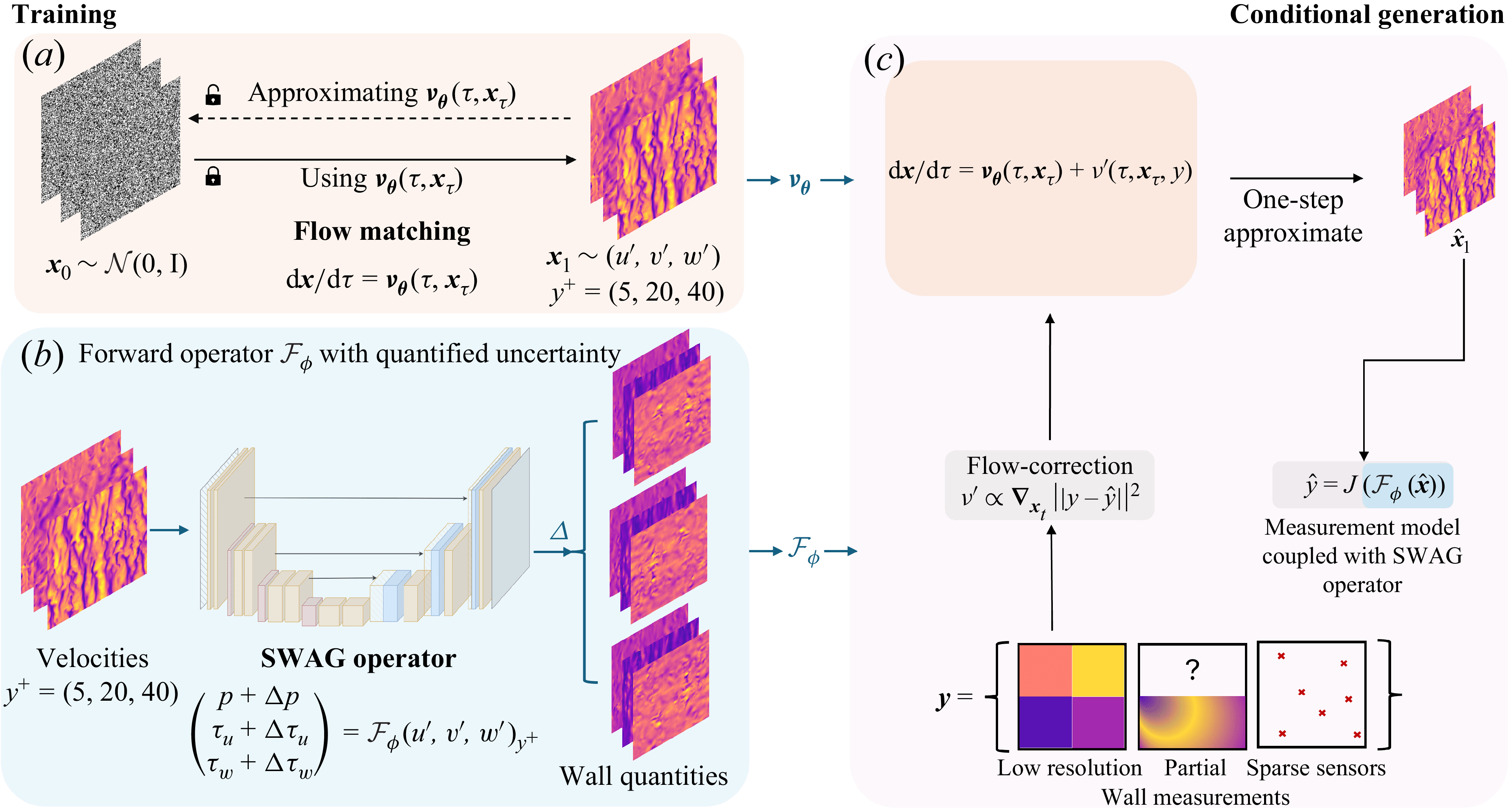


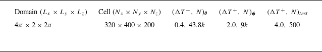
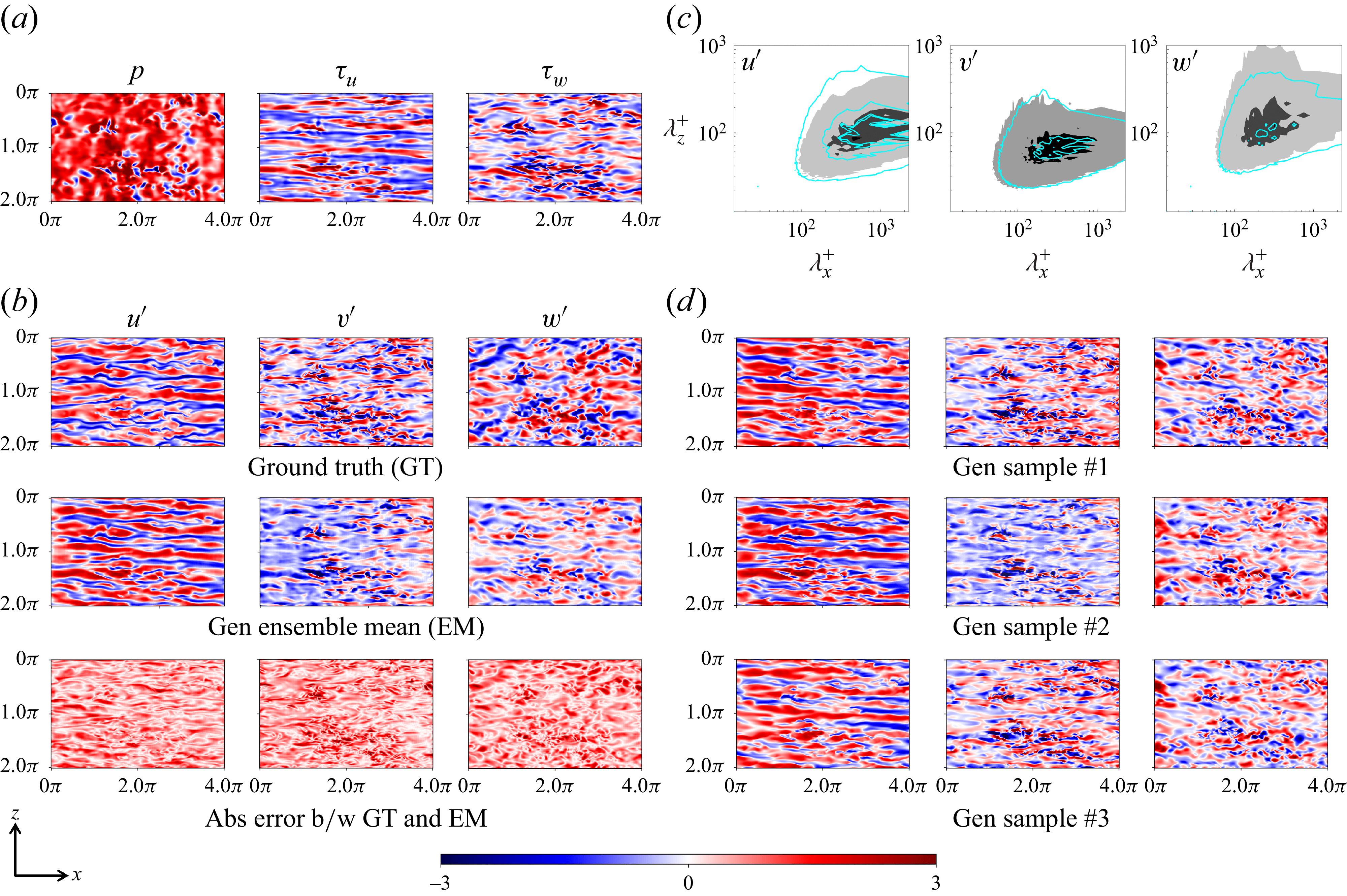


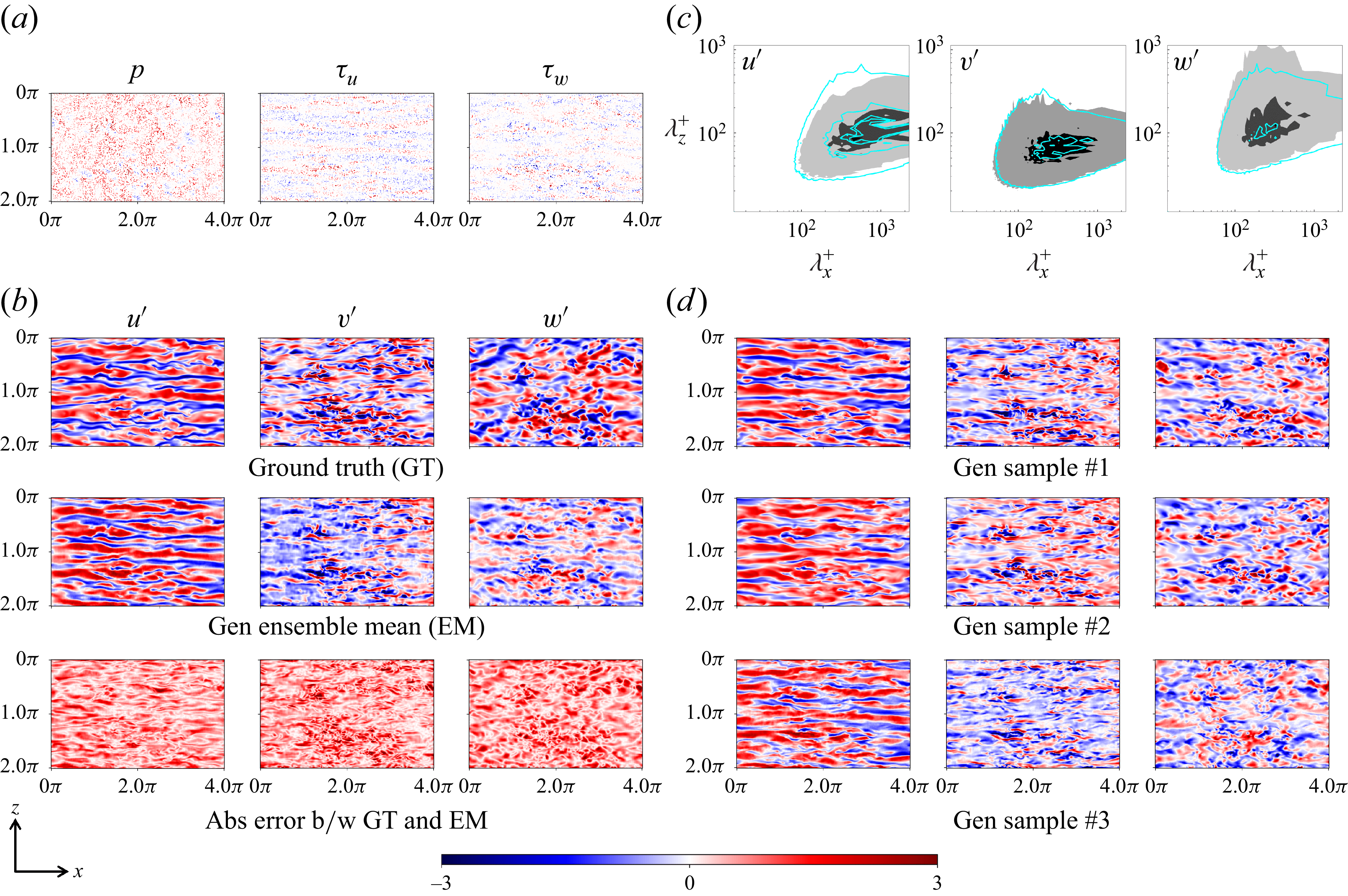


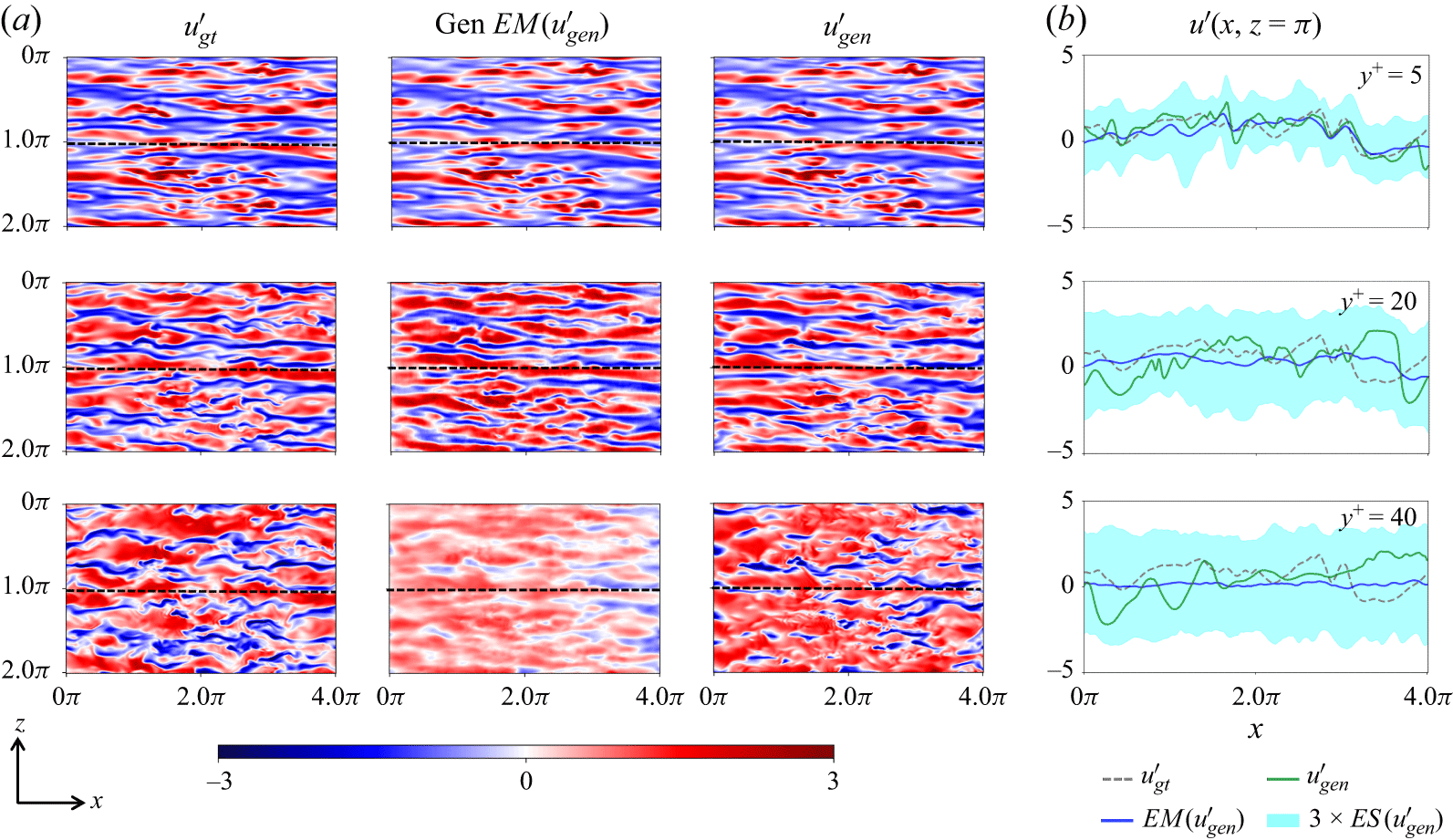


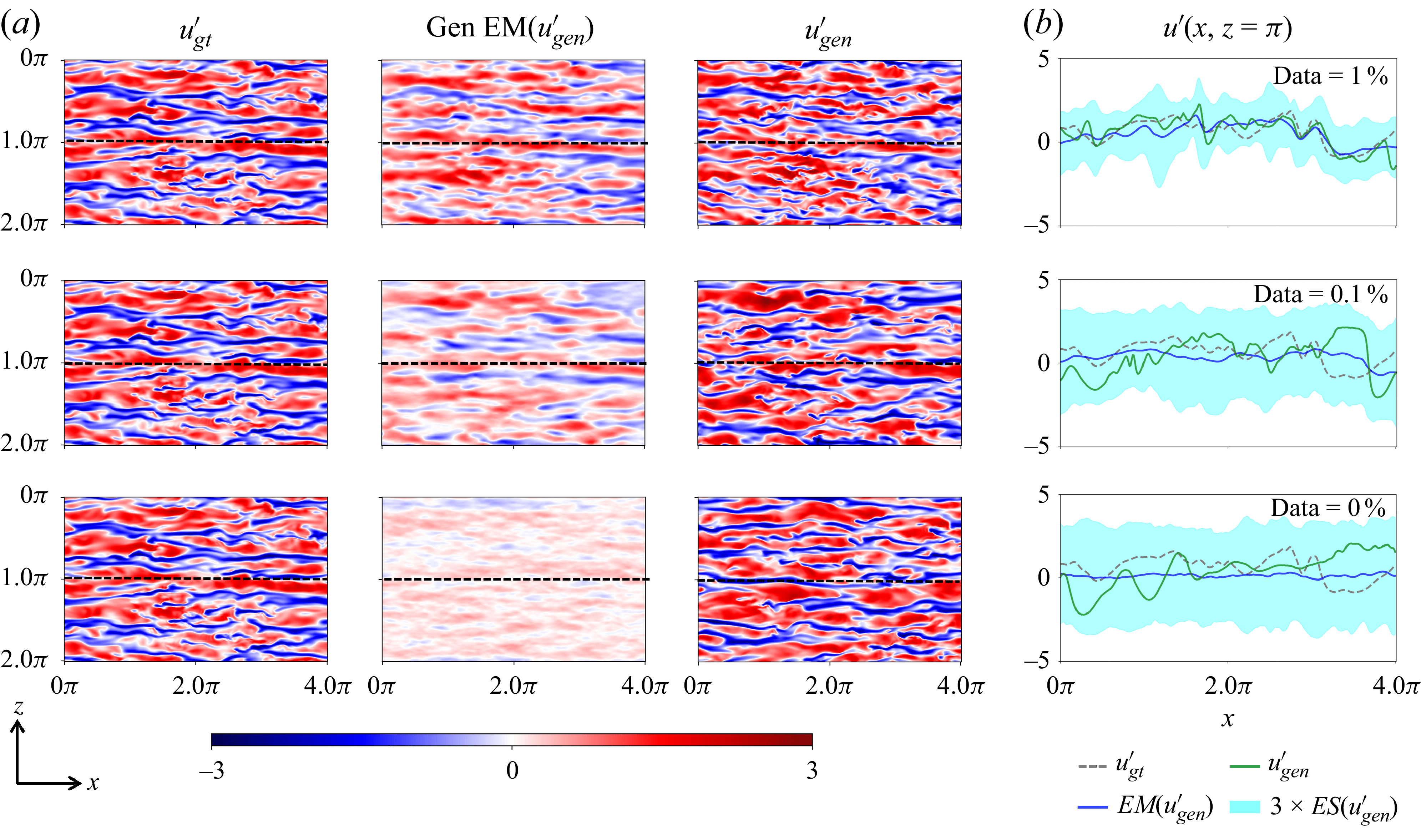


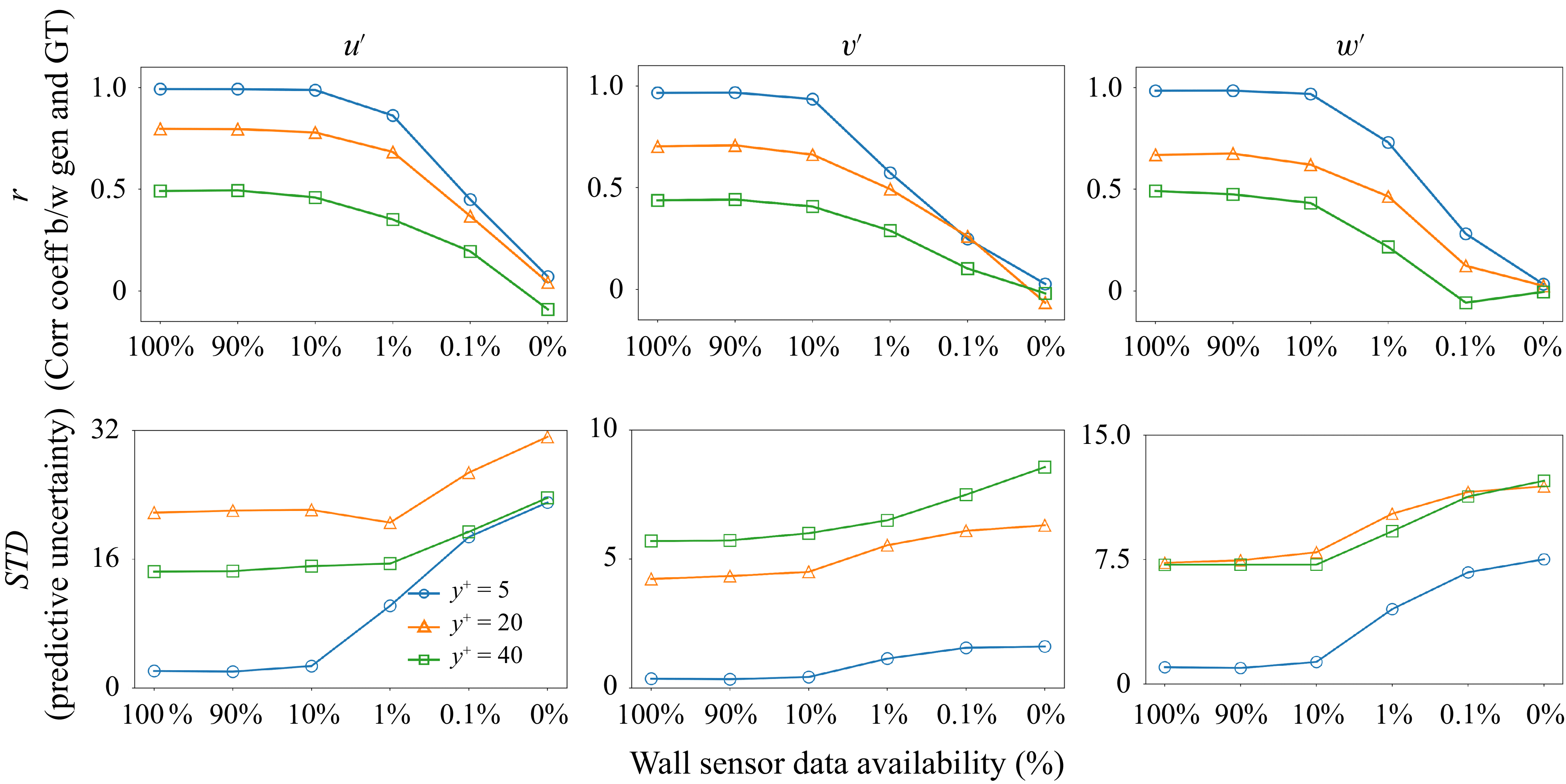


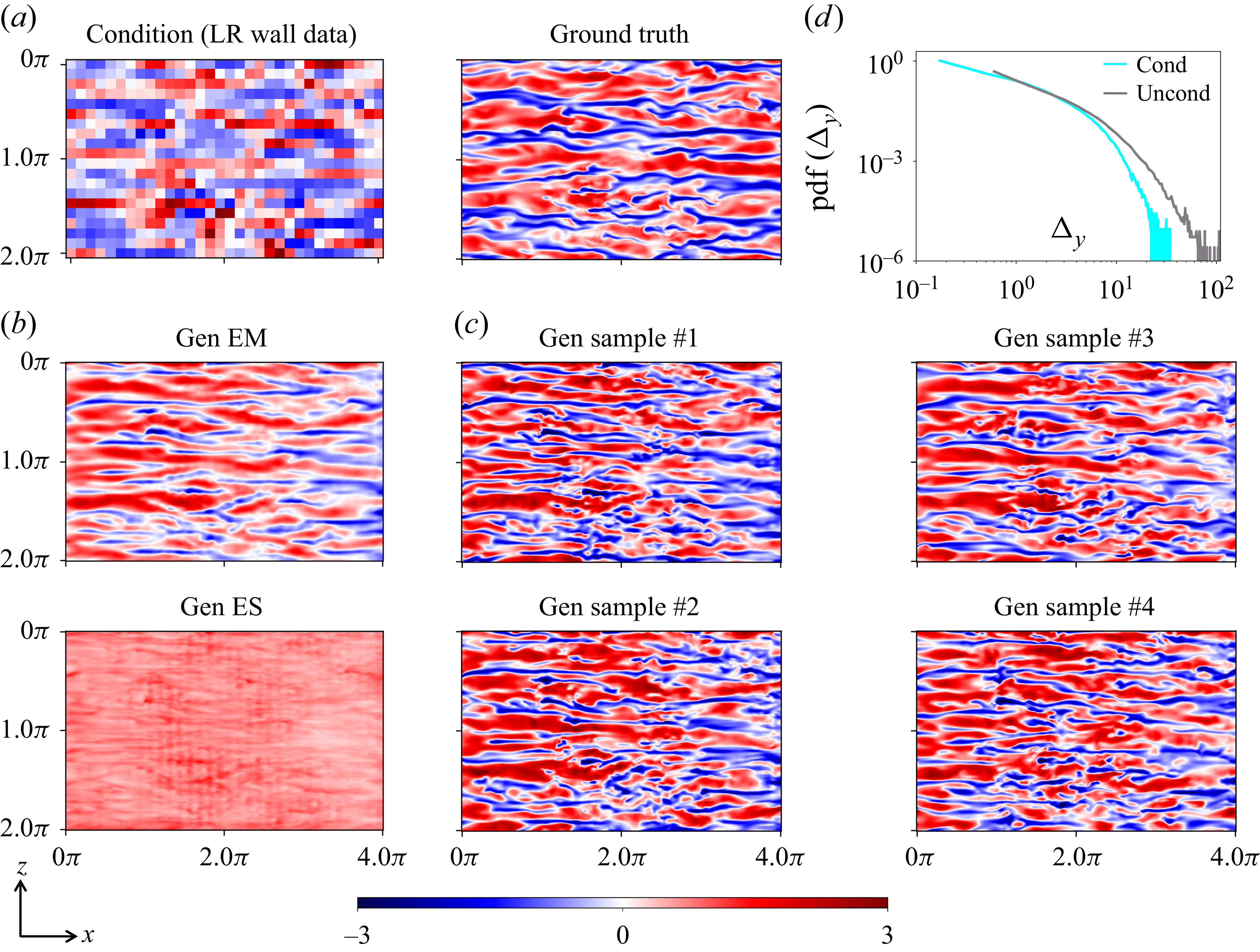


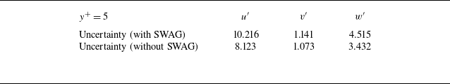


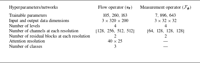


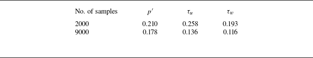


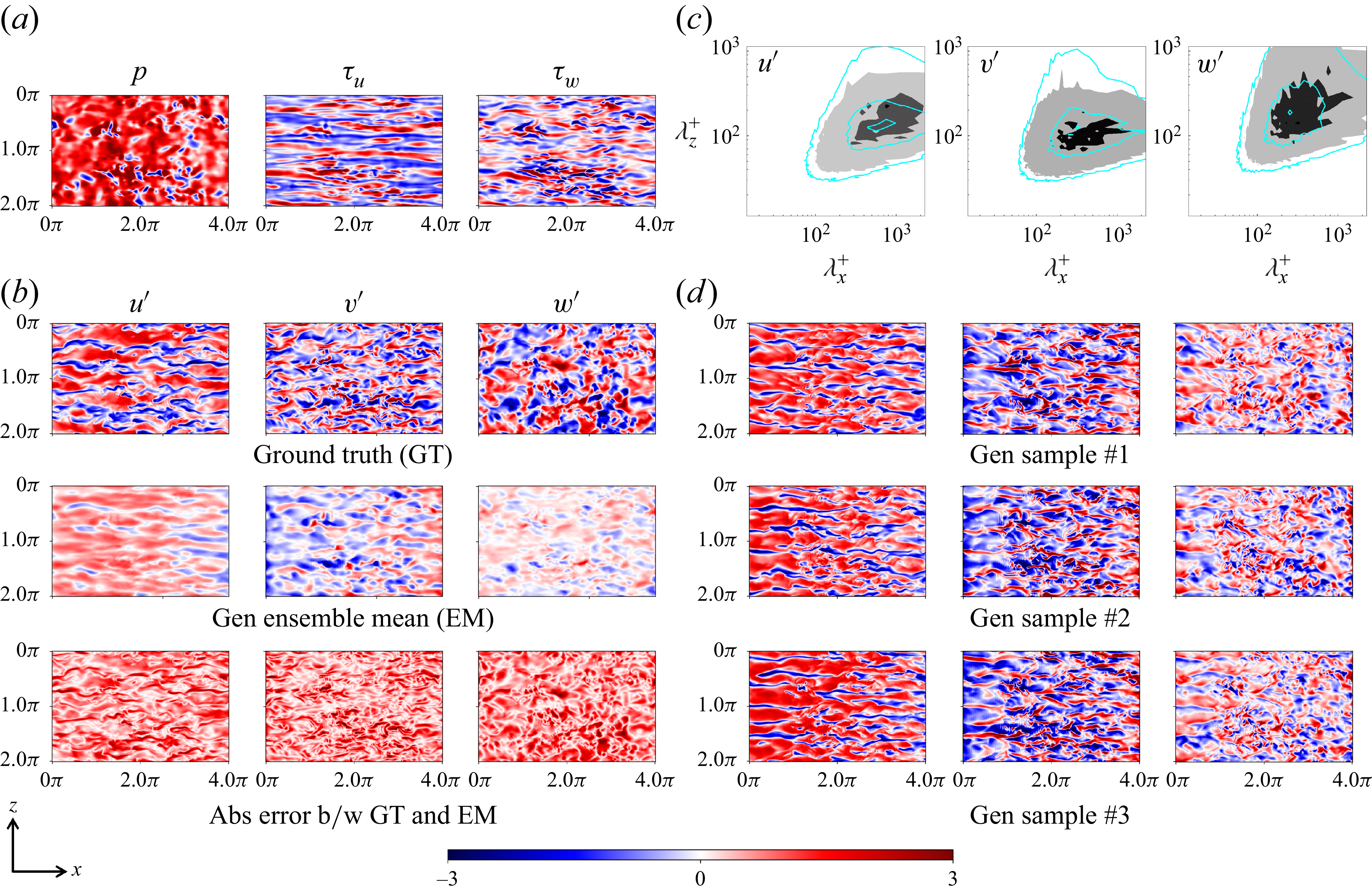


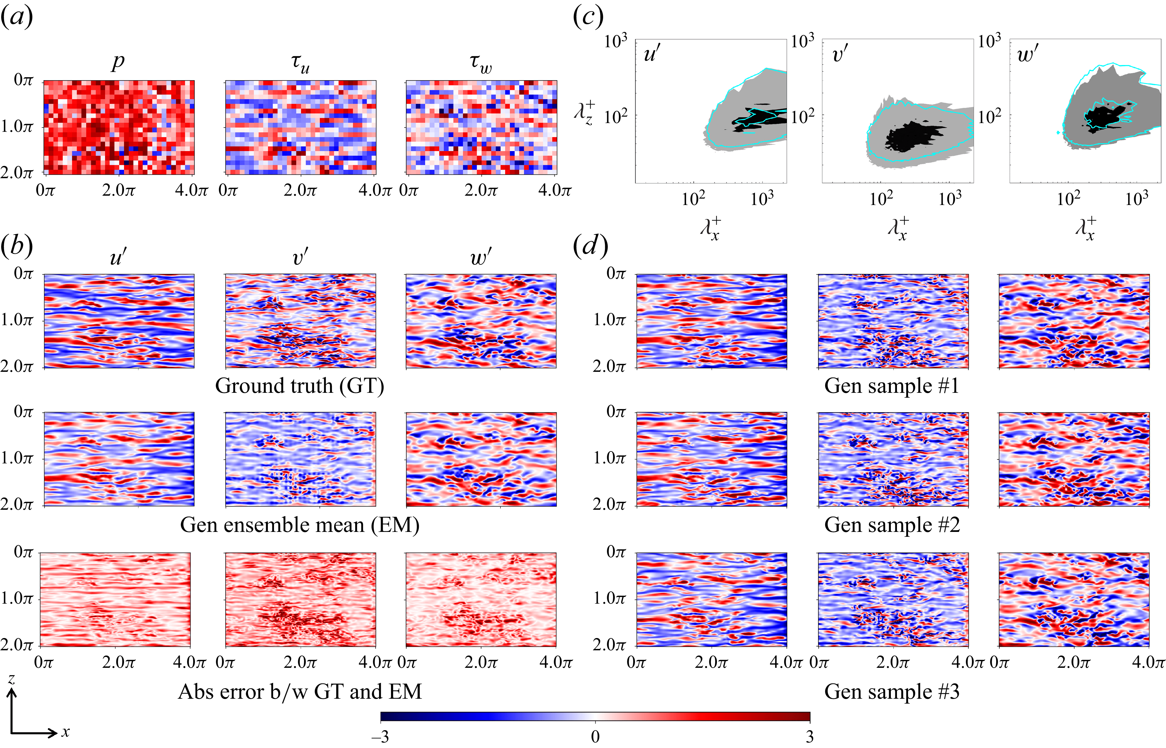


 Open access