


1. Introduction
We study the effects of long-run inflation in a model with competitive search and non-degenerate money distribution. Monetary search models provide a deeper microfoundation of money, where important market frictions or behavioral outcomes are not assumed but are consequences of environmental (e.g., informational and contractual) imperfections. The framework has been applied to answer many questions such as the existence and essentiality of money, financial intermediation, asset liquidity, and equilibrium price dispersion.Footnote 1
In this paper, we follow and extend the model of Menzio et al. (Reference Menzio, Shi and Sun2013) to study non-zero inflation. The heterogeneity in our model is a result of equilibrium directed search and matching frictions. That is, we do not rely on exogenous shocks to individual states, and, as in Menzio et al. (Reference Menzio, Shi and Sun2013), possible persistence in agent heterogeneity is induced by endogenous individual spending cycles.Footnote 2 However, a question remains open in this class of competitive-search models: How does inflation affect the trade-off underlying heterogenous individuals’ matching and market participation rates, their corresponding terms of trade, and the resulting equilibrium distribution of agents’ money holdings? This question is very relevant now as most advanced economies are facing higher inflation rates in recent times.Footnote 3
In our model, individuals direct their search to sellers, and sellers post their trade terms in anticipation of different matching probabilities at different trading posts (or submarkets). These incentives and matching probabilities, in turn, depend on different levels of money holdings and inflation policy. This introduces a different channel of monetary policy that is muted in models without this endogenous mechanism. Consequently, we have equilibrium-determined distributions of market participation, market tightness, relative prices, and trade quantities.Footnote 4 Addressing our question is an important first step towards incorporating competitive search behavior into a more feature-laden and quantitative model.
With competitive search, it is well known that individuals face a trade-off between an extensive margin of trading probability and an intensive margin of trade quantity (see, e.g., Wright et al. Reference Wright, Kircher, Julien and Guerrieri2021; Rocheteau and Wright Reference Rocheteau and Wright2005; Moen Reference Moen1997). We emphasize that with a non-degenerate distribution of money balances in equilibrium, the effects of inflation on these trade-offs in our model depend on agents’ money holdings. We provide a numerical comparative study of steady-state equilibria across two inflation regimes to illustrate the results (see Section 4).Footnote 5 In particular, we show that with higher long run inflation, while matching probabilities fall with inflation for all agents, agents with relatively lower money balances (“the poor”) face a steeper decline in payments and matching probabilities than those with higher money holdings (“the rich”).Footnote 6 This translates to an increase in dispersion of total payments and trading probabilities as inflation becomes higher.Footnote 7
The difference in the steepness (with respect to higher inflation regimes) of the decline in matching probabilities and payment amounts between the “rich” and “poor” reflects the underlying tension between the intensive and extensive margin in the competitive search markets. This tension or trade-off varies depending on the agent’s money holding. Our equilibrium comparisons show that the “rich,” relative to the “poor” will also have a higher velocity of spending (i.e., a higher ratio of expected payments per dollar carried) due to the flatter decline in matching rates and payments. This enables the “rich” to replenish their liquidity faster to support better matching and trade outcomes in goods search markets as inflation rises, compared to the “poor.”
Higher inflation has two effects on agents’ money holdings. On one hand, higher inflation tends to compress dispersion in money holding. That comes from the intensive margin effect. This is typically known as the redistributive effect of the inflation tax and is a common feature in all heterogeneous-agent monetary models (see, for example, Erosa and Ventura Reference Erosa and Ventura2002). On the other hand, with higher inflation, the extensive margin aspect of competitive search gives us a rising dispersion in heterogeneous matching opportunities, spending amounts, and speeds of transactions. These gaps between the “rich” and “poor” widen with inflation and deliver an opposing force against the standard redistributive effect of inflation tax. When inflation is low, the intensive margin effect dominates, while the extensive margin effect becomes stronger at sufficiently high inflation rates. This leads to a novel non-monotonic relationship between inflation and money-holding inequality: For low long-run inflation rates, the inequality in money holdings tends to diminish with inflation. However, for sufficiently high inflation rates, the inequality in money holdings increases with inflation.Footnote 8
As a consequence of this friction working against the compressing or redistributive effect of inflation, the welfare cost of inflation is nontrivial, especially when transitional dynamics are taken into account. In standard models, due to its redistributive property, the welfare cost of inflation is lowered relative to a representative-agent monetary model. With competitive search, this effect can be dominated by the effects of inflation on the extensive margin of trade. As a result, we find that the welfare cost of inflation can be as high as, or even higher than, the original representative-agent calculation of Lucas Reference Lucas2000.Footnote 9
Finally, we also develop a novel way of solving the equilibrium computationally. There is a technical challenge posed by the theoretical work of Menzio et al. (Reference Menzio, Shi and Sun2013): The agents’ ex-ante value function (labeled as $B$
later) induced by pure strategies with competitive search is typically non-concave/convex over multiple parts of its domain (money holdings). Thus, agents can be better off by choosing lotteries that convexify the graph of
$B$
later) induced by pure strategies with competitive search is typically non-concave/convex over multiple parts of its domain (money holdings). Thus, agents can be better off by choosing lotteries that convexify the graph of $B$
. We propose a practical, efficient, and high-precision implementation of this idea using standard convex hull computational tools.Footnote
10
We explain this idea further in Section 3.1 and in more detail in Online Appendix E.
$B$
. We propose a practical, efficient, and high-precision implementation of this idea using standard convex hull computational tools.Footnote
10
We explain this idea further in Section 3.1 and in more detail in Online Appendix E.
1.1. Related literature
Our paper uses a competitive search framework to study the effects of inflation. There is a vast literature analyzing the effects of inflation. We briefly review some of them here while paying more attention to papers more closely related to our approach. We then discuss a few papers which also feature non-degenerate distributions of money holdings and emphasize the difference between our model and theirs. Finally, we describe the essence of Menzio et al. Reference Menzio, Shi and Sun2013, and discuss why it poses an open problem for us to study here in terms of inflation and its distribution and welfare effects.Footnote 11
1.1.1. Inflation, heterogeneity and money distribution
Consider a taxonomy of the costs and benefits of inflation in standard Walrasian-market models (see, e.g., Erosa and Ventura Reference Erosa and Ventura2002). First, inflation acts as an intertemporal tax that distorts consumption. This feature raises the (welfare) cost of inflation in all monetary models (with or without heterogeneous agents). Second, inflation is costly since agents have to engage in precautionary liquidity management activities. Third, inflation may act as a redistributive tax that shifts resources from the “rich” to the “poor.” This force tends to lower the welfare cost of inflation.
In most heterogeneous-agent models (see, e.g., Imrohoroğlu and Prescott Reference Imrohoroğlu and Prescott1991a; Akyol Reference Akyol2004; Boel and Camera Reference Boel and Camera2009; Meh et al. Reference Meh, Ríos-Rull and Terajima2010), the redistributive-tax channel of inflation is strong. This is often because there is only an intensive margin through which inflation tax works.Footnote 12 That is, with higher inflation, agents would like to reduce their money holdings. Those with high money balances reduce their holdings more relative to those at the bottom end of the distribution. This tends to lower the average money balance. Hence, inflation acts as a progressive tax that reduces inequality of money holdings. This explains why in many heterogeneous-agent models, the welfare cost of inflation is often smaller than representative-agent models (Camera and Chien Reference Camera and Chien2014).Footnote 13
In a random-matching, search-theoretic model of money, Molico (Reference Molico2006) shows that as inflation increases agents choose to pay more money in decentralized trades and a higher amount of money is paid per unit of the good.Footnote 14 This “real balance effect” can work against the redistributive effect of inflation. There is a similar effect in our model, but with a different underlying twist. In our setting with competitive search in decentralized trades, this is bolstered by the additional extensive margin effect: Higher inflation exacts a greater downside risk of not matching for agents by reducing the equilibrium matching probability for buyers. Although expected money carried in each decentralized trade will be lower per payment for goods, with lower equilibrium probability of matching, agents who get matched don’t have to reduce consumption as much. This trade-off between matching probability and quantity of goods in the competitive search environment (see, e.g., Peters Reference Peters1984, Reference Peters1991; Moen Reference Moen1997; Burdett et al. Reference Burdett, Shi and Wright2001; Julien et al. Reference Julien, Kennes and King2008; Shi Reference Shi and Shi2008) amplifies the speed at which agents expect to deplete their money in decentralized trades.
Chiu and Molico (Reference Chiu and Molico2010) also have a notion of extensive margin, in the form of costly participation in centralized markets. In our setting, even without costly participation in markets, there is a non-trivial extensive margin. In Chiu and Molico (Reference Chiu and Molico2010) and Rocheteau et al. (Reference Rocheteau, Weill and Wong2021), trading probabilities are fixed in decentralized-market meetings. This is due to their random matching assumption. In our setting, the extensive margin arises in the form of endogenous matching probabilities.
Jin and Zhu (Reference Jin and Zhu2022) also consider the effect of long-run inflation in a random-matching model (Trejos and Wright Reference Trejos and Wright1995; Shi Reference Shi1995). In their setting, agents can only hold indivisible amounts of money. Furthermore, the inflation policy in their framework is indirectly determined through an abstract fiscal tax-and-transfer scheme that is conditioned on individual wealth. In our setting, we take the anonymity of agents literally and do not presume that government policy has such superior informational advantage. Moreover, our setting is closer to the latest generation of monetary search models where goods and assets are divisible. This allows the models to be more amenable to empirical calibration and quantitative work.
1.1.2. Money and competitive search
In contrast to the Walrasian or random matching models discussed above, our Menzio et al. (Reference Menzio, Shi and Sun2013) competitive search setup advances another channel to the standard taxonomy previously outlined.Footnote 15 The essence of their model is as follows: Suppose all agents begin in the economy as identical individuals. In one period, each agent has to make a decision whether to enter a centralized market (CM) to work and re-balance their money holdings, or to direct their search in a decentralized market (DM). In the search problem agents direct themselves to different trading posts with different terms of trade and matching probabilities. Firms anticipate that and create these trading posts accordingly. In equilibrium, there is an asymptotic distribution of heterogenous money holdings that must be consistent with the agents’ different responses in trading probabilities, payments and market participation rates. Menzio et al. (Reference Menzio, Shi and Sun2013) characterize such an equilibrium in the special case of zero long-run inflation.
Our paper complements Menzio et al. (Reference Menzio, Shi and Sun2013). We study how inflation drives agents’ competitive search trade-offs, their endogenous market participations, and how this ties in with distributional outcomes. In our model, the responsiveness of agents in terms of their trading probabilities and quantities is endogenous. We show that because of the Menzio et al. (Reference Menzio, Shi and Sun2013) heterogeneity in matching rates, there is an opposing extensive margin effect that helps to mitigate the previously-discussed redistributive channel of inflation.Footnote 16 With higher inflation, agents are also spending faster in decentralized trades and entering the centralized market to rebalance their liquidity more frequently. Higher centralized-market participation implies that there are more agents with less money holding at the end of each period. These agents will enter the centralized market in the subsequent period. Also, there will be a smaller measure of agents at the upper end of the distribution since they top up with less liquidity in the centralized market and spend faster in the decentralized search market.
Endogenous matching probabilities via competitive search is not new (see, e.g., Rocheteau and Wright Reference Rocheteau, Wright, Rocheteau and Wright2009, Reference Rocheteau and Wright2005; Lagos and Rocheteau Reference Lagos and Rocheteau2005). What is different here is that the endogenous matching probabilities are heterogeneous in agent states and its distribution depends on inflation. This creates a nontrivial equilibrium, countervailing effect to what would be a traditional redistributive role of inflation. This is an important feature driving our non-monotone inequality results.Footnote 17 In addition to the introduction and study of inflation, we differ slightly from Menzio et al. (Reference Menzio, Shi and Sun2013) by including quasi-linear utility of consumption and labor in the CM. This is done to enable a more flexible way to calibrate the model to data. It does not qualitatively alter the mechanism in Menzio et al. (Reference Menzio, Shi and Sun2013).
Sun and Zhou (Reference Sun and Zhou2018) also embed the competitive search market of Menzio et al. (Reference Menzio, Shi and Sun2013) to study fiscal and monetary policy. However, there is a crucial difference between their model and Menzio et al. (Reference Menzio, Shi and Sun2013), and thus our study of inflation here. They assumed away the endogenous duration of an agent’s participation of the DM in the original Menzio et al. (Reference Menzio, Shi and Sun2013) paper. Agents in their model can only stay for one period in the DM and must return to the CM (featuring quasilinear preferences) afterwards. Their model would be a version of the competitive search equilibrium in Rocheteau and Wright (Reference Rocheteau and Wright2005) where there is a degenerate distribution of money and prices, if not for an assumption that agents in the CM draw an (i.i.d.) idiosyncratic income shock.Footnote 18 As a consequence, a one-shot and non-persistent dispersion in matching probabilities in Sun and Zhou (Reference Sun and Zhou2018) is entirely buttressed by an assumption of exogenous heterogeneity in individual labor-supply productivities. In contrast, we follow Menzio et al. (Reference Menzio, Shi and Sun2013) where ex-post heterogeneity arises in conjunction with equilibrium competitive-search dispersion in trading posts. This allows us to connect inflation policy to what we call the extensive margin underlying the distributional outcome, through agents’ heterogeneous market participation and duration of such participation, and their transactions’ speed.
The remainder of this paper is organized as follows. In Section 2, we set up and analyze a version of the model of Menzio et al. (Reference Menzio, Shi and Sun2013) in a more general setting with non-zero inflation. In Section 3, we discuss our contribution in terms of a novel computational solution approach and also our calibration of the model. In Section 4, we conduct the main study on how inflation affects the equilibrium trade-offs that drive the model’s distributional and welfare outcomes. We do so by comparing monetary equilibria under alternative long-run inflation policies. In section 5, we compute the welfare cost of inflation implied by this model. We conclude with Section 6.
2. The model
The model builds on Menzio et al. (Reference Menzio, Shi and Sun2013). Time is discrete and indexed by $t\in \mathbb{N}$
. Hereinafter, we will denote
$t\in \mathbb{N}$
. Hereinafter, we will denote $X\,:\!=\,X_{t}$
and
$X\,:\!=\,X_{t}$
and $X_{+1}\,:\!=\,X_{t+1}$
for dynamic variables. There is one general good denoted by
$X_{+1}\,:\!=\,X_{t+1}$
for dynamic variables. There is one general good denoted by $C$
. There are also
$C$
. There are also $I$
types of specific goods indexed by
$I$
types of specific goods indexed by $i\in {1,2,\ldots \ldots, I}$
, where
$i\in {1,2,\ldots \ldots, I}$
, where $I\geqslant 3.$
Agents in the economy consist of
$I\geqslant 3.$
Agents in the economy consist of $I$
types individuals,
$I$
types individuals, $I$
types of firms, and a government that implements a (long-run) inflation target through controlling money-supply growth. There are measure one of each type
$I$
types of firms, and a government that implements a (long-run) inflation target through controlling money-supply growth. There are measure one of each type $i$
individuals,
$i$
individuals, $i\in I$
. An individual
$i\in I$
. An individual $i$
consumes the general good
$i$
consumes the general good $C$
, the specific good
$C$
, the specific good $i$
and produces good
$i$
and produces good $i+1$
(mod-
$i+1$
(mod- $\left |I\right |$
) as well as the general good
$\left |I\right |$
) as well as the general good $C$
. For firms, each type
$C$
. For firms, each type $i$
firm,
$i$
firm, $i\in I,$
consists of a large number of firms. A type
$i\in I,$
consists of a large number of firms. A type $i$
firm produces type
$i$
firm produces type $i$
good as well as the general good
$i$
good as well as the general good $C.$
As in Menzio et al. (Reference Menzio, Shi and Sun2013), firms are owned by the individuals through a balanced mutual fund.
$C.$
As in Menzio et al. (Reference Menzio, Shi and Sun2013), firms are owned by the individuals through a balanced mutual fund.
There is a centralized market (CM) and a decentralized market (DM). The CM is a competitive Walrasian market where the individuals supply labor $l$
, and, consume the general good
$l$
, and, consume the general good $C$
. As a result, they also manage their liquidity holding
$C$
. As a result, they also manage their liquidity holding $y$
to be carried into the following period. In the DM where the specific
$y$
to be carried into the following period. In the DM where the specific $i$
goods are traded, we have a setting similar to Menzio et al. (Reference Menzio, Shi and Sun2013). There is an information friction: Buyers of special DM goods are anonymous and cannot trade using private claims or contracts with selling firms. As a result, the only medium of exchange is money. For each type-
$i$
goods are traded, we have a setting similar to Menzio et al. (Reference Menzio, Shi and Sun2013). There is an information friction: Buyers of special DM goods are anonymous and cannot trade using private claims or contracts with selling firms. As a result, the only medium of exchange is money. For each type- $i$
good, there is a continuum of submarkets indexed by the terms of trade
$i$
good, there is a continuum of submarkets indexed by the terms of trade $(x,q)\in \mathbb{R}_{+}^{2}$
, where
$(x,q)\in \mathbb{R}_{+}^{2}$
, where $x$
is a real payment by a buyer and
$x$
is a real payment by a buyer and $q$
is the quantity traded in exchange. Hereinafter, the explicit dependency on the type of good
$q$
is the quantity traded in exchange. Hereinafter, the explicit dependency on the type of good $i\in I$
will become unnecessary.Footnote
19
Each
$i\in I$
will become unnecessary.Footnote
19
Each $i$
-type firm commits to posted terms of trade in all submarkets it chooses to enter. Buyers of good
$i$
-type firm commits to posted terms of trade in all submarkets it chooses to enter. Buyers of good $i$
direct their search toward these submarkets that sell good
$i$
direct their search toward these submarkets that sell good $i$
, by choosing the best terms of trade offered. However, as we will see, these buyers will have to balance their decision on terms of trades against the probability of getting matched. Since firms and buyers choose which submarket to participate in, a type
$i$
, by choosing the best terms of trade offered. However, as we will see, these buyers will have to balance their decision on terms of trades against the probability of getting matched. Since firms and buyers choose which submarket to participate in, a type $i$
buyer will only participate in the submarkets where type
$i$
buyer will only participate in the submarkets where type $i$
firms sell.
$i$
firms sell.
At any date, each individual decides which market—CM or DM—to participate in. An individual can only be in the CM or DM at a given time period. Firms operate in both CM and DM at the same time. Individuals demand money as a precaution against the need for liquidity in anonymous markets in the DM. A firm in the CM hires labor to produce the general CM good and the special DM goods. A type $i$
firm hires labor service from type
$i$
firm hires labor service from type $i-1$
(mod-
$i-1$
(mod- $\left |I\right |$
) individuals (in the CM spot labor market) and transforms it (linearly) into the same amount of DM good
$\left |I\right |$
) individuals (in the CM spot labor market) and transforms it (linearly) into the same amount of DM good $i$
.
$i$
.
Two features of the model give rise to market incompleteness: First, equilibrium matching in the DM (where money is essential) implies that agents face ex-ante uncertainty over being able to exchange and consume in those markets. Second, in the equilibria that emerge, there is endogenous limited participation in centralized markets. Since agents are anonymous in the DM, their individual risks are uninsurable: private state-contingent securities are not incentive feasible. Anonymity renders equilibrium value for money as a medium of exchange. Competitive search and matching with options to participate in the CM yields equilibrium-determined ex-post agent heterogeneity.

Figure 1. Timing, markets, outcomes.
Figure 1 summarizes the timing of events and decisions between two arbitrary dates. Next, we detail the model primitives and decision problems.
2.1. Individuals, matching and firms
2.1.1. Preference representation
The per-period utility function of an individual is
 \begin{equation} U\left (C\right )-h\left (l\right )+u(q). \end{equation}
where $U(C)$
is the utility of consuming the general good
$U(C)$
is the utility of consuming the general good $C$
,
$C$
, $h(l)$
is the disutility from supplying labor in the CM, and
$h(l)$
is the disutility from supplying labor in the CM, and $u(q)$
is the utility of consuming the specific good in the DM. We assume that the functions
$u(q)$
is the utility of consuming the specific good in the DM. We assume that the functions $U$
and
$U$
and $u$
are continuously differentiable, strictly increasing, strictly concave,
$u$
are continuously differentiable, strictly increasing, strictly concave, $U_{1},u_{1}\gt 0$
,
$U_{1},u_{1}\gt 0$
, $U_{11},u_{11}\lt 0$
, and the following boundary conditions hold:
$U_{11},u_{11}\lt 0$
, and the following boundary conditions hold: $u(0)=U_{1}(\infty )=u_{1}(\infty )=0$
, and
$u(0)=U_{1}(\infty )=u_{1}(\infty )=0$
, and $u_{1}(0)\lt \infty$
.Footnote
20
Also, we assume that
$u_{1}(0)\lt \infty$
.Footnote
20
Also, we assume that $h\left (l\right )=l$
. This simplifies the algebraic description of the CM decision problem and ensures that agents exiting the CM are identical.
$h\left (l\right )=l$
. This simplifies the algebraic description of the CM decision problem and ensures that agents exiting the CM are identical.
2.1.2. Matching technology in the DM
Let $\theta \in \mathbb{R}_{+}$
denote the ratio of trading posts to buyers in a submarket—i.e., its market tightness. In a submarket with tightness
$\theta \in \mathbb{R}_{+}$
denote the ratio of trading posts to buyers in a submarket—i.e., its market tightness. In a submarket with tightness $\theta$
, the probability that a buyer is matched with a trading post is
$\theta$
, the probability that a buyer is matched with a trading post is $b=\lambda (\theta )$
. The probability a trading post is matched with a buyer is
$b=\lambda (\theta )$
. The probability a trading post is matched with a buyer is $s={{\rho }({\theta }) \,:\!=\,}\lambda (\theta )/\theta$
. We assume that the function
$s={{\rho }({\theta }) \,:\!=\,}\lambda (\theta )/\theta$
. We assume that the function $\lambda :\mathbb{R}_{+}\rightarrow [0,1]$
is strictly increasing, with
$\lambda :\mathbb{R}_{+}\rightarrow [0,1]$
is strictly increasing, with $\lambda (0)=0$
, and
$\lambda (0)=0$
, and $\lambda (\infty )=1.$
The function
$\lambda (\infty )=1.$
The function $\rho (\theta )$
is strictly decreasing, with
$\rho (\theta )$
is strictly decreasing, with $\rho (0)=1$
, and
$\rho (0)=1$
, and $\rho (\infty )=0.$
We can re-write a trading post’s matching probability
$\rho (\infty )=0.$
We can re-write a trading post’s matching probability $s=\rho (\theta )=\rho \circ \lambda ^{-1}(b)\equiv \mu (b)$
. Observe that the matching function
$s=\rho (\theta )=\rho \circ \lambda ^{-1}(b)\equiv \mu (b)$
. Observe that the matching function $\mu$
is a decreasing function, and that
$\mu$
is a decreasing function, and that $\mu (0)=1$
and
$\mu (0)=1$
and $\mu (1)=0$
. Assume that
$\mu (1)=0$
. Assume that $1/\mu (b)$
is strictly convex in
$1/\mu (b)$
is strictly convex in $b$
.
$b$
.
2.1.3. Firms
Consider a firm of type $i\in I$
that takes the CM good’s relative price
$i\in I$
that takes the CM good’s relative price $p$
(in units of labor) as given. Following Menzio et al. (Reference Menzio, Shi and Sun2013), we define labor as the numéraire good. The firm hires labor on the spot market to produce the CM good and the DM good. One unit of labor is transformed into one unit of CM good linearly. In the DM, a firm takes the market tightness function
$p$
(in units of labor) as given. Following Menzio et al. (Reference Menzio, Shi and Sun2013), we define labor as the numéraire good. The firm hires labor on the spot market to produce the CM good and the DM good. One unit of labor is transformed into one unit of CM good linearly. In the DM, a firm takes the market tightness function $\theta$
as given, and chooses the measure of trading posts (viz., shops)
$\theta$
as given, and chooses the measure of trading posts (viz., shops) $\text{d}N(x,q)$
to open in each submarket.Footnote
21
If
$\text{d}N(x,q)$
to open in each submarket.Footnote
21
If $x$
is what a matched buyer is willing to pay for
$x$
is what a matched buyer is willing to pay for $q$
and
$q$
and $s(x,q)\,:\!=\,\rho \left (\theta \left (x,q\right )\right )$
, then
$s(x,q)\,:\!=\,\rho \left (\theta \left (x,q\right )\right )$
, then $x\cdot s(x,q)$
is the firm’s expected revenue in submarket
$x\cdot s(x,q)$
is the firm’s expected revenue in submarket $(x,q)$
. To produce
$(x,q)$
. To produce $q$
the firm must hire
$q$
the firm must hire $c(q)$
units of labor. Hence
$c(q)$
units of labor. Hence $s(x,q)c(q)$
is its expected labor wage bill in submarket
$s(x,q)c(q)$
is its expected labor wage bill in submarket $(x,q)$
. We assume that
$(x,q)$
. We assume that $q\mapsto c(q)$
is a continuous convex function. The firm also pays a per-period fixed cost
$q\mapsto c(q)$
is a continuous convex function. The firm also pays a per-period fixed cost $k$
of creating the trading post in submarket
$k$
of creating the trading post in submarket $(x,q)$
.
$(x,q)$
.
The firm’s profit is:
 \begin{equation} \pi (p;\,k)=\max _{Y\in \mathbb{R}_{+}}\left \{ pY-Y\right \} +\max _{\text{d}N}\int _{\mathbb{R}_{+}^{2}}\left \{ s(x,q)\left [x-c(q)\right ]-k\right \} \text{d}N(x,q), \end{equation}
where $N$
is a positive measure on the Borel
$N$
is a positive measure on the Borel $\sigma$
-algebra
$\sigma$
-algebra $\mathcal{B}\left (\mathbb{R}_{+}^{2}\right )$
. The first term on the RHS is the firm’s value from operating in the CM. The second is its DM total expected value across all submarkets it chooses to operate in.
$\mathcal{B}\left (\mathbb{R}_{+}^{2}\right )$
. The first term on the RHS is the firm’s value from operating in the CM. The second is its DM total expected value across all submarkets it chooses to operate in.
Note that the firms’ problem above (and also agents’ decision problems to be discussed below) do not explicitly depend on the aggregate distribution of agents. This is because of the nature of competitive search in the DM: Firms and buyers take matching probabilities as given when making their respective price posting and directed search decisions. The observed terms of trade posts and matching probabilities suffice to condition their decision processes. Moreover, CM preferences are quasilinear such that agents are identical at the end of the CM. We discuss this further in Section 2.4.1.
2.2. Money supply
At the start of each date $t$
, the total stock of money in the economy
$t$
, the total stock of money in the economy $M$
is known. We assume that
$M$
is known. We assume that $M$
grows at a constant rate
$M$
grows at a constant rate $\tau$
:
$\tau$
:
 \begin{equation} \frac {M_{+1}}{M}=1+\tau, \end{equation}
We assume $\tau \gt \beta -1$
, where
$\tau \gt \beta -1$
, where $\beta$
is the discount factor. New money stock
$\beta$
is the discount factor. New money stock $\tau M$
is injected lump sum to all agents at the end of date
$\tau M$
is injected lump sum to all agents at the end of date $t$
.
$t$
.
Since we define labor as the numéraire good, if we denote $\omega M$
as the current nominal wage rate, where
$\omega M$
as the current nominal wage rate, where $\omega$
is normalized nominal wage (i.e., nominal wage rate per units of
$\omega$
is normalized nominal wage (i.e., nominal wage rate per units of $M$
), then a dollar’s worth of money is equivalent to
$M$
), then a dollar’s worth of money is equivalent to $1/\omega M$
units of labor. The variable
$1/\omega M$
units of labor. The variable $\omega$
will be endogenously determined in a monetary equilibrium.Footnote
22
If
$\omega$
will be endogenously determined in a monetary equilibrium.Footnote
22
If $M$
is the beginning-of-period aggregate stock of money in circulation, then
$M$
is the beginning-of-period aggregate stock of money in circulation, then $1/\omega =M\times 1/\omega M$
is the beginning-of-period real aggregate (per-capita) stock of money, measured in units of labor.
$1/\omega =M\times 1/\omega M$
is the beginning-of-period real aggregate (per-capita) stock of money, measured in units of labor.
Denote (equilibrium) nominal wage growth as $\gamma (\tau )\equiv \omega _{+1}M_{+1}/(\omega M)$
. Later, for a stationary monetary equilibrium, we will require that equilibrium nominal wage grows at the same rate as money supply, i.e.,
$\gamma (\tau )\equiv \omega _{+1}M_{+1}/(\omega M)$
. Later, for a stationary monetary equilibrium, we will require that equilibrium nominal wage grows at the same rate as money supply, i.e., $\gamma (\tau )\vert _{\left (\omega _{+1}=\omega \right )}=M_{+1}/M$
.
$\gamma (\tau )\vert _{\left (\omega _{+1}=\omega \right )}=M_{+1}/M$
.
2.3. Individuals’ decisions
An individual is identified by her current money balance, $m$
(measured in units of labor). Given policy
$m$
(measured in units of labor). Given policy $\tau$
, her decisions also depend on the aggregate wage
$\tau$
, her decisions also depend on the aggregate wage $\omega$
. Denote the relevant state vector as
$\omega$
. Denote the relevant state vector as $\textbf{s}\,:\!=\,(m,\omega )$
.Footnote
23
At the beginning of a period (ex ante), an individual decides either to work and consume in the CM or to be a buyer in the frictional DM.Footnote
24
Next, we describe the decision problems of agents who are ex-post CM or DM buyers. We then describe an agent’s ex-ante decision problem of choosing which of CM or DM to go to.
$\textbf{s}\,:\!=\,(m,\omega )$
.Footnote
23
At the beginning of a period (ex ante), an individual decides either to work and consume in the CM or to be a buyer in the frictional DM.Footnote
24
Next, we describe the decision problems of agents who are ex-post CM or DM buyers. We then describe an agent’s ex-ante decision problem of choosing which of CM or DM to go to.
2.3.1. Ex-post CM buyers
Suppose now we have an individual $\textbf{s}\,:\!=\,(m,\omega )$
who begins the current period in the CM. The individual takes policy,
$\textbf{s}\,:\!=\,(m,\omega )$
who begins the current period in the CM. The individual takes policy, $\tau$
, and the sequence of aggregate prices,
$\tau$
, and the sequence of aggregate prices, $\left (\omega, \omega _{+1},\ldots \right )$
, as given. Her value from optimally consuming
$\left (\omega, \omega _{+1},\ldots \right )$
, as given. Her value from optimally consuming $C$
, supplying labor
$C$
, supplying labor $l$
, and accumulating end-of-period money balance
$l$
, and accumulating end-of-period money balance $y$
, is
$y$
, is
 \begin{align} W(\textbf{s})=\max _{\left (C,l,y\right )\in \mathbb{R}_{+}^{3}}\biggl \{ U(C)-h(l)+\beta \bar {V}\left (\textbf{s}_{+1}\right ):pC+y\leq m+l,\ \ m_{+1}=\frac {\omega y+\tau }{\omega _{+1}\left (1+\tau \right )}\biggr \}, \end{align}
where $\bar {V}:S\rightarrow \mathbb{R}$
is her continuation value function (see Section 2.3.3 on the following page). This continuation value function yields her next-period expected total payoff from state
$\bar {V}:S\rightarrow \mathbb{R}$
is her continuation value function (see Section 2.3.3 on the following page). This continuation value function yields her next-period expected total payoff from state $m_{+1}$
. The continuation state for the individual,
$m_{+1}$
. The continuation state for the individual, $m_{+1}$
, is derived as follows: At the end of the CM, the individual would have accumulated balance
$m_{+1}$
, is derived as follows: At the end of the CM, the individual would have accumulated balance $y$
(measured in units of labor). In current units of nominal money, this is
$y$
(measured in units of labor). In current units of nominal money, this is $\omega M\times y$
. At the beginning of next period, each individual gets a nominal transfer of new money
$\omega M\times y$
. At the beginning of next period, each individual gets a nominal transfer of new money $\tau M$
. In units of labor next period, the beginning-of-period balance would thus be
$\tau M$
. In units of labor next period, the beginning-of-period balance would thus be $m_{+1}=\left (\omega My+\tau M\right )/\left (\omega _{+1}M_{+1}\right )$
. Replacing for
$m_{+1}=\left (\omega My+\tau M\right )/\left (\omega _{+1}M_{+1}\right )$
. Replacing for $M/M_{+1}$
with the money supply process in (2.3) gives the expression for the individual’s continuation state
$M/M_{+1}$
with the money supply process in (2.3) gives the expression for the individual’s continuation state $m_{+1}$
in (2.4).
$m_{+1}$
in (2.4).
2.3.2. Ex-post DM buyers
Now we focus on an individual who has just decided to be a DM buyer. The buyer chooses which submarket (or trading post) $\left (x,q\right )$
to enter, taking the market tightness function
$\left (x,q\right )$
to enter, taking the market tightness function $\left (x,q\right )\mapsto \theta \left (x,q\right )$
as given. The individual buyer,
$\left (x,q\right )\mapsto \theta \left (x,q\right )$
as given. The individual buyer, $\textbf{s}\,:\!=\,(m,\omega )$
, has initial value:Footnote
25
$\textbf{s}\,:\!=\,(m,\omega )$
, has initial value:Footnote
25
 \begin{align} B(\textbf{s})&=\max _{x\in [0,m],q\in \mathbb{R}_{+}}\left \{ \beta \left [1-b\left (x,q\right )\right ]\left [\bar {V}\left (\frac {\omega m+\tau }{\omega _{+1}\left (1+\tau \right )},\omega _{+1}\right )\right ]\right .\nonumber \\ &\quad +\left .b\left (x,q\right )\left [u(q)+\beta \bar {V}\left (\frac {\omega \left (m-x\right )+\tau }{\omega _{+1}\left (1+\tau \right )},\omega _{+1}\right )\right ]\right \} . \end{align}
Consider the first two terms on the RHS of Equation (2.5): With probability $1-b\left (x,q\right )\boldsymbol{\,:\!=\,}1-\lambda \left (\theta \left (x,q\right )\right )$
the buyer fails to match with the trading post and must thus continue the next period with his initial money balance subject to inflationary transfer. With the complementary probability
$1-b\left (x,q\right )\boldsymbol{\,:\!=\,}1-\lambda \left (\theta \left (x,q\right )\right )$
the buyer fails to match with the trading post and must thus continue the next period with his initial money balance subject to inflationary transfer. With the complementary probability $b\left (x,q\right )\,:\!=\,\lambda \left (\theta \left (x,q\right )\right )$
he matches with a trading post
$b\left (x,q\right )\,:\!=\,\lambda \left (\theta \left (x,q\right )\right )$
he matches with a trading post $\left (x,q\right )$
, pays the seller
$\left (x,q\right )$
, pays the seller $x$
in exchange for a flow payoff
$x$
in exchange for a flow payoff $u\left (q\right )$
, and then continues into the next period with his net balance, also subject to inflationary transfers.
$u\left (q\right )$
, and then continues into the next period with his net balance, also subject to inflationary transfers.
2.3.3. Ex-ante
Given a money balance $z$
, the individual decides which markets to participate in, and her value becomes
$z$
, the individual decides which markets to participate in, and her value becomes
 \begin{equation} \tilde {V}\left (z,\omega \right )=\max _{a\in \left \{ 0,1\right \} }\left \{ aW\left (z,\omega \right )+\left (1-a\right )B\left (z,\omega \right )\right \} . \end{equation}
As shown in Menzio et al. (Reference Menzio, Shi and Sun2013), the resulting value function $B$
in Equation (2.5) may not be strictly concave in
$B$
in Equation (2.5) may not be strictly concave in $m$
.Footnote
26
This is the case even if primitive functions are strictly concave. As a result, the value function
$m$
.Footnote
26
This is the case even if primitive functions are strictly concave. As a result, the value function $\tilde {V}$
may not be concave either.Footnote
27
This implies that agents can be weakly better off by choosing a lottery over the pure participation outcomes. Suppose at the beginning of a period, an agent begins with money balance
$\tilde {V}$
may not be concave either.Footnote
27
This implies that agents can be weakly better off by choosing a lottery over the pure participation outcomes. Suppose at the beginning of a period, an agent begins with money balance $m$
. If there is a non-empty subset
$m$
. If there is a non-empty subset $\left [z_{1},z_{2}\right ]$
containing
$\left [z_{1},z_{2}\right ]$
containing $m$
such that any weighted average of the pure-action induced values
$m$
such that any weighted average of the pure-action induced values $\tilde {V}(z_{1},\omega )$
and
$\tilde {V}(z_{1},\omega )$
and $\tilde {V}(z_{2},\omega )$
(weakly) dominates
$\tilde {V}(z_{2},\omega )$
(weakly) dominates $\tilde {V}(m,\omega )$
, then the agent will optimally play a fair lottery
$\tilde {V}(m,\omega )$
, then the agent will optimally play a fair lottery $\left (\pi _{1},1-\pi _{1}\right )$
over the prizes
$\left (\pi _{1},1-\pi _{1}\right )$
over the prizes $\left \{ z_{1},z_{2}\right \}$
. This yields the ex-ante value
$\left \{ z_{1},z_{2}\right \}$
. This yields the ex-ante value
 \begin{equation} \bar {V}\left (\textbf{s}\right )=\max _{\pi _{1}\in [0,1],z_{1},z_{2}}\left \{ \pi _{1}\tilde {V}(z_{1},\omega )+\left (1-\pi _{1}\right )\tilde {V}\left (z_{2},\omega \right ):\,\pi _{1}z_{1}+(1-\pi _{1})z_{2}=m\right \} . \end{equation}
2.4. Monetary equilibrium
In this paper, we restrict attention to the case of a monetary equilibrium. Hereinafter, whenever we refer to “monetary equilibrium,” or “equilibrium,” we mean a (Markovian) monetary equilibrium—one in which agent’s decision functions are time-invariant maps. In what follows, we first characterize the equilibrium strategy of firms (section 2.4.1), the equilibrium value and decision functions of agents in the CM (section 2.4.2) and in the DM (section 2.4.3), and then we describe the market clearing conditions in equilibrium (section 2.4.4). At the end of this section, we define formally the notion of a stationary monetary equilibrium (SME).
2.4.1. Equilibrium strategy of firms
A firm’s problem is static. We can characterize the equilibrium behavior of a firm given $p$
(in the CM). Free entry in the CM will render zero profits to firms in equilibrium, and thus,
$p$
(in the CM). Free entry in the CM will render zero profits to firms in equilibrium, and thus, $p=1$
. Likewise, free entry and zero-profit in the DM with competitive search imply that
$p=1$
. Likewise, free entry and zero-profit in the DM with competitive search imply that
 \begin{equation} r(x,q)\,:\!=\,s\left (\theta (x,q)\right )\left [x-c(q)\right ]-k\leq 0,\qquad \text{and,}\qquad \theta (x,q)\geq 0, \end{equation}
where the weak inequalities would hold with complementary slackness: For a submarket $(x,q)$
such that
$(x,q)$
such that $r(x,q)\lt 0$
, the firm optimally chooses not to post in the submarket. If
$r(x,q)\lt 0$
, the firm optimally chooses not to post in the submarket. If $r(x,q)=0$
, then the firm is indifferent to creating different numbers of trading posts in submarket
$r(x,q)=0$
, then the firm is indifferent to creating different numbers of trading posts in submarket $(x,q)$
. We can also deduce that
$(x,q)$
. We can also deduce that $r(x,q)\gt 0$
cannot be an equilibrium: If expected profit is positive, then this implies
$r(x,q)\gt 0$
cannot be an equilibrium: If expected profit is positive, then this implies $\theta (x,q)=+\infty$
, and thus
$\theta (x,q)=+\infty$
, and thus $s\left (\theta (x,q)\right )=0$
which yields a contradiction to the case.Footnote
28
We will restrict attention to an equilibrium where Equation (2.8) also holds for submarkets not visited by any buyer.Footnote
29
$s\left (\theta (x,q)\right )=0$
which yields a contradiction to the case.Footnote
28
We will restrict attention to an equilibrium where Equation (2.8) also holds for submarkets not visited by any buyer.Footnote
29
From (2.8), we can deduce that
 \begin{equation} s(x,q)\equiv \mu \circ b\left (x,q\right )=\begin{cases} \frac {k}{x-c(q)} & \iff x-c(q)\gt k\\ 1 & \iff x-c(q)\leq k \end{cases}. \end{equation}
Observe that the firm’s probability of matching with a buyer, $s(x,q)\,:\!=\,\rho \left (\theta \left (x,q\right )\right )$
depends only on the posted terms of trade
$s(x,q)\,:\!=\,\rho \left (\theta \left (x,q\right )\right )$
depends only on the posted terms of trade $(x,q)$
. Likewise, the buyer’s probability of matching with a firm is
$(x,q)$
. Likewise, the buyer’s probability of matching with a firm is $b(x,q)\,:\!=\,\lambda \left (\theta \left (x,q\right )\right )$
, for a given the matching technology
$b(x,q)\,:\!=\,\lambda \left (\theta \left (x,q\right )\right )$
, for a given the matching technology $\mu :[0,1]\rightarrow [0,1]$
. Thus, in any submarket with positive measure of buyers, the market tightness,
$\mu :[0,1]\rightarrow [0,1]$
. Thus, in any submarket with positive measure of buyers, the market tightness, $\theta (x,q)\equiv b(x,q)/s(x,q)$
, is necessarily and sufficiently determined by free entry into the submarket. Moreover, the terms of trade of a submarket
$\theta (x,q)\equiv b(x,q)/s(x,q)$
, is necessarily and sufficiently determined by free entry into the submarket. Moreover, the terms of trade of a submarket $(x,q)$
is sufficient to identify the submarket. This implies that firms’ and agents’ optimal decision processes do not depend on the equilibrium distribution of agents. They only depend on the distribution through the aggregate statistic
$(x,q)$
is sufficient to identify the submarket. This implies that firms’ and agents’ optimal decision processes do not depend on the equilibrium distribution of agents. They only depend on the distribution through the aggregate statistic $\omega$
as a result of inflation. The equilibrium will be (partially) block recursive.
$\omega$
as a result of inflation. The equilibrium will be (partially) block recursive.
In equilibrium, there is a relation between $q$
and
$q$
and $(x,b)$
. That is, in any equilibrium, each active trading post will produce and trade the quantity:
$(x,b)$
. That is, in any equilibrium, each active trading post will produce and trade the quantity:
 \begin{equation} q=Q(x,b)\equiv c^{-1}\left [x-\frac {k}{\mu (b)}\right ], \end{equation}
given payment $x$
and its matching probability
$x$
and its matching probability $s=\mu (b)$
. This relation allows us to perform a change of variables, and re-write the buyers’ problems below in terms choices over
$s=\mu (b)$
. This relation allows us to perform a change of variables, and re-write the buyers’ problems below in terms choices over $(x,b)$
, instead of over
$(x,b)$
, instead of over $(x,q)$
.
$(x,q)$
.
2.4.2. Equilibrium CM individual
Denote $\mathcal{C}[0,\bar {m}]$
as the set of continuous and increasing functions with domain
$\mathcal{C}[0,\bar {m}]$
as the set of continuous and increasing functions with domain $[0,\bar {m}]$
. Let
$[0,\bar {m}]$
. Let $\mathcal{V}[0,\bar {m}]\subset \mathcal{C}[0,\bar {m}]$
be the set of continuous, increasing and concave functions on the domain
$\mathcal{V}[0,\bar {m}]\subset \mathcal{C}[0,\bar {m}]$
be the set of continuous, increasing and concave functions on the domain $[0,\bar {m}]$
.
$[0,\bar {m}]$
.
Proposition 1 (CM value and decision functions)
Assume $\tau /\omega \lt \bar {m}$
. For a given sequence of prices
$\tau /\omega \lt \bar {m}$
. For a given sequence of prices $\left \{ \omega, \omega _{+1},\ldots \right \}$
, the value function of the individual beginning in the CM,
$\left \{ \omega, \omega _{+1},\ldots \right \}$
, the value function of the individual beginning in the CM, $W\left (\cdot, \omega \right )$
, has the following properties:
$W\left (\cdot, \omega \right )$
, has the following properties:
-
1. $W\left (\cdot, \omega \right )\in \mathcal{V}[0,\bar {m}]$
, i.e., it is continuous, increasing and concave on
$\left [0,\bar {m}\right ]$
. Moreover, it is linear on
$\left [0,\bar {m}\right ]$
.
$W\left (\cdot, \omega \right )\in \mathcal{V}[0,\bar {m}]$
, i.e., it is continuous, increasing and concave on
$\left [0,\bar {m}\right ]$
. Moreover, it is linear on
$\left [0,\bar {m}\right ]$
. -
2. The partial derivative functions
$W_{1}\left (\cdot, \omega \right )$
and
$\bar {V}_{1}\left (\cdot, \omega _{+1}\right )$
exist and satisfy the first-order condition(2.11)and the envelope condition:
\begin{equation} \frac {\beta }{1+\tau }\left (\frac {\omega }{\omega _{+1}}\right )\bar {V}_{1}\left (\frac {\omega y^{\star }\left (m,\omega \right )+\tau }{\omega _{+1}\left (1+\tau \right )},\omega _{+1}\right )\begin{cases} \leq 1, & y^{\star }\left (m,\omega \right )\geq 0\\ \geq 1, & y^{\star }\left (m,\omega \right )\leq y_{\text{max}}\left (\omega ;\tau \right ) \end{cases}, \end{equation}
(2.12)where
\begin{equation} W_{1}\left (m,\omega \right )=1, \end{equation}
$y^{\star }(m,\omega )=m+l^{\star }(m,\omega )-C^{\star }(m,\omega )$
,
$l^{\star }(m,\omega )$
and
$C^{\star }(m,\omega )$
, respectively, are the associated optimal choices on labor effort and consumption in the CM.
-
3. The stationary Markovian policy rules
$y^{\star }\left (\cdot, \omega \right )$
and
$l^{\star }\left (\cdot, \omega \right )$
are scalar-valued and continuous functions on
$\left [0,\bar {m}\right ]$
.


-
(a) The function
$y^{\star }\left (\cdot, \omega \right )$
, is constant valued on
$\left [0,\bar {m}\right ]$
. -
(b) The optimizer
$l^{\star }\left (\cdot, \omega \right )$
is an affine and decreasing function on
$\left [0,\bar {m}\right ]$
. -
(c) Moreover, for every
$\left (m,\omega \right )$
, the optimal choice
$l^{\star }(m,\omega )$
is interior:
$0\lt l_{\min }\leq l^{\star }\left (m\right )\leq l_{\max }\left (\omega ;\,\tau \right )\lt +\infty$
, where there is a very small
$l_{\text{min}}\gt 0$
and
$l_{max}\left (\omega \right )\,:\!=\,y_{\text{max}}\left (\omega ;\,\tau \right )+U^{-1}\left (1\right )\lt 2U^{-1}\left (1\right )\in \left (0,\infty \right )$
.


In Proposition 1, we provide an extension of the results of Menzio et al. (Reference Menzio, Shi and Sun2013) on CM individuals’ value and policy functions to the case with non-zero inflation. (Its proof is relegated to Online Appendix B. The proposition says the following: First, $W\left (\cdot, \omega \right )\in \mathcal{V}[0,\bar {m}]$
is continuous, increasing and concave on
$W\left (\cdot, \omega \right )\in \mathcal{V}[0,\bar {m}]$
is continuous, increasing and concave on $\left [0,\bar {m}\right ]$
, and it is linear on
$\left [0,\bar {m}\right ]$
, and it is linear on $\left [0,\bar {m}\right ]$
. Second, the partial derivative functions
$\left [0,\bar {m}\right ]$
. Second, the partial derivative functions $W_{1}\left (\cdot, \omega \right )$
and
$W_{1}\left (\cdot, \omega \right )$
and $\bar {V}_{1}\left (\cdot, \omega _{+1}\right )$
exist and satisfy a first-order condition. Third, agents’ optimal money balance and labor decision rules, respectively,
$\bar {V}_{1}\left (\cdot, \omega _{+1}\right )$
exist and satisfy a first-order condition. Third, agents’ optimal money balance and labor decision rules, respectively, $y^{\star }\left (\cdot, \omega \right )$
and
$y^{\star }\left (\cdot, \omega \right )$
and $l^{\star }\left (\cdot, \omega \right )$
are scalar-valued and continuous functions on
$l^{\star }\left (\cdot, \omega \right )$
are scalar-valued and continuous functions on $\left [0,\bar {m}\right ]$
, and their selections are always interior. Also, for a fixed
$\left [0,\bar {m}\right ]$
, and their selections are always interior. Also, for a fixed $\omega$
, the graph of
$\omega$
, the graph of $y^{\star }\left (\cdot, \omega \right )$
is downward sloping and that of
$y^{\star }\left (\cdot, \omega \right )$
is downward sloping and that of $l^{\star }\left (\cdot, \omega \right )$
is constant-valued or flat. We also derive the equilibrium decisions of the CM agent.
$l^{\star }\left (\cdot, \omega \right )$
is constant-valued or flat. We also derive the equilibrium decisions of the CM agent.
2.4.3. Equilibrium DM buyer
Observe that since $\bar {V}(\cdot, \omega ),W(\cdot, \omega )\in \mathcal{V}[0,\bar {m}]$
(i.e., are continuous, increasing and concave), then by (A.1),
$\bar {V}(\cdot, \omega ),W(\cdot, \omega )\in \mathcal{V}[0,\bar {m}]$
(i.e., are continuous, increasing and concave), then by (A.1), $\bar {V}\left (\cdot, \omega \right )\in \mathcal{V}[0,\bar {m}]$
. In an equilibrium, the DM buyer’s problem in (2.5) can be re-written as
$\bar {V}\left (\cdot, \omega \right )\in \mathcal{V}[0,\bar {m}]$
. In an equilibrium, the DM buyer’s problem in (2.5) can be re-written as
 \begin{align} B(\textbf{s})=\max _{x\in [0,m],b\in [0,1]}\biggl \{\beta (1-b)\left [\bar {V}\left (\frac {\omega m+\tau }{\omega _{+1}\left (1+\omega \right )},\omega _{+1}\right )\right ]\nonumber \\ +b\biggl [u\left (Q(x,b)\right )+\beta \bar {V}\left (\frac {\omega \left (m-x\right )+\tau }{\omega _{+1}\left (1+\tau \right )},\omega _{+1}\right )\biggr ]\biggr \}. \end{align}
It appears as if the buyer is choosing his matching probability $b$
along with payment
$b$
along with payment $x$
. This is comes from a change of variables utilizing the equilibrium relation (2.10) between quantity
$x$
. This is comes from a change of variables utilizing the equilibrium relation (2.10) between quantity $q$
and terms of trade
$q$
and terms of trade $(x,b)$
. From this we can begin to see that there will be a trade-off to the buyer, in terms of an extensive margin (i.e., trading opportunity
$(x,b)$
. From this we can begin to see that there will be a trade-off to the buyer, in terms of an extensive margin (i.e., trading opportunity $b$
), and, an intensive margin (i.e., trading quantity given payment
$b$
), and, an intensive margin (i.e., trading quantity given payment $x$
).
$x$
).
The operator defined by (2.13) does not preserve concavity: The objective function in (2.13) is not jointly concave in the decisions $\left (x,b\right )$
and state
$\left (x,b\right )$
and state $m$
, since it is bilinear in the function
$m$
, since it is bilinear in the function $b$
and the value function
$b$
and the value function $\bar {V}$
, or the flow payoff function
$\bar {V}$
, or the flow payoff function $u$
. However, using lattice programming arguments, we can still show that the resulting DM buyers’ optimal choice functions for
$u$
. However, using lattice programming arguments, we can still show that the resulting DM buyers’ optimal choice functions for $(x,b)$
, denoted by
$(x,b)$
, denoted by $\left (x^{\star },b^{\star }\right )$
, are monotone, continuous, and have unique selections.
$\left (x^{\star },b^{\star }\right )$
, are monotone, continuous, and have unique selections.
Proposition 2 (DM value and decision functions)
For a given price sequence $\left \{ \omega, \omega _{+1},\ldots \right \}$
, the following properties hold.
$\left \{ \omega, \omega _{+1},\ldots \right \}$
, the following properties hold.
-
1. For any
$\bar {V}(\cdot, \omega _{+1})\in \mathcal{V}\left [0,\bar {m}\right ]$
, the DM buyer’s value function is increasing and continuous in money balances,
$B\left (\cdot, \omega \right )\in \mathcal{C}\left [0,\bar {m}\right ]$
. -
2. For any
$m\leq k$
, DM buyers’ optimal decisions are
$b^{\star }\left (m,\omega \right )=x^{\star }\left (m,\omega \right )=q^{\star }\left (m,\omega \right )=0$
, and
$B\left (m,\omega \right )=\beta \bar {V}\left [\phi (m,\omega ),\omega _{+1}\right ]$
, where
$\phi (m,\omega )\,:\!=\,(\omega m+\tau )/\left [\omega _{+1}(1+\tau )\right ]$
. -
3. At any
$\left (m,\omega \right )$
, where
$m\in \left [k,\bar {m}\right ]$
and the buyer matching probability is positive
$b^{\star }\left (m,\omega \right )\gt 0$
:


-
(a) The optimal selections
$\left (x^{\star },b^{\star },q^{\star }\right )(m,\omega )$
and
$\phi ^{\star }(m,\omega )\,:\!=\,\phi \left [m-x^{\star }\left (m,\omega \right ),\omega \right ]$
, are unique, continuous, and increasing in
$m$
. -
(b) The buyer’s marginal valuation of money
$B_{1}(m,\omega )$
exists if and only if the marginal ex-ante value of money
$\bar {V}_{1}\left [\phi (m,\omega ),\omega \right ]$
exists. -
(c)
$B(m,\omega )$
is strictly increasing in
$m$
. -
(d) the optimal policy functions
$b^{\star }$
and
$x^{\star }$
, respectively, satisfy the first-order conditions(2.14)and,
\begin{align} &u\circ Q\left [x^{\star }(m,\omega ),b^{\star }(m,\omega )\right ]+b^{\star }(m,\omega )\left (u\circ Q\right )_{2}\left [x^{\star }(m,\omega ),b^{\star }(m,\omega )\right ] \nonumber \\ &\quad =\beta \left [\bar {V}\left (\phi \left (m,\omega \right ),\omega _{+1}\right )-\bar {V}\left (\phi ^{\star }\left (m,\omega \right ),\omega _{+1}\right )\right ], \end{align}
(2.15)
\begin{equation} \left (u\circ Q\right )_{1}\left [x^{\star }(m,\omega ),b^{\star }(m,\omega )\right ]=\frac {\beta }{1+\tau }\left (\frac {\omega }{\omega _{+1}}\right )\bar {V}_{1}\left [\phi ^{\star }(m,\omega ),\omega _{+1}\right ]. \end{equation}


Proposition 2 states the properties of a DM agent’s value and policy functions. It extends the results from Menzio et al. (Reference Menzio, Shi and Sun2013) to the setting with non-zero inflation. The proof is given in the appendix, we summarize the idea of the proof: Part 1 of the proposition states that $B\left (\cdot, \omega \right )\in \mathcal{C}\left [0,\bar {m}\right ]$
is increasing and continuous in
$B\left (\cdot, \omega \right )\in \mathcal{C}\left [0,\bar {m}\right ]$
is increasing and continuous in $m$
. This observation uses standard results from optimization and is contained in Lemma 1 of the appendix. Part 2 is proven in Lemma 2 in the appendix, and its insight here is simple: If buyers do not carry enough money to at least pay for a trading post’s fixed cost, no firm will want to set up that post in equilibrium, and so the buyers get nothing. Part 3(a) is proven in Lemma 3 using the fact that a log-transform of a DM buyer’s objective function is jointly concave in the choice variables
$m$
. This observation uses standard results from optimization and is contained in Lemma 1 of the appendix. Part 2 is proven in Lemma 2 in the appendix, and its insight here is simple: If buyers do not carry enough money to at least pay for a trading post’s fixed cost, no firm will want to set up that post in equilibrium, and so the buyers get nothing. Part 3(a) is proven in Lemma 3 using the fact that a log-transform of a DM buyer’s objective function is jointly concave in the choice variables $\left (x,b\right )$
, and is continuous in
$\left (x,b\right )$
, and is continuous in $m$
(fixing the aggregate state
$m$
(fixing the aggregate state $\omega$
). It nevertheless satisfies an increasing difference—and therefore, supermodularity—property. Thus, by lattice programming arguments, we can show that the DM buyer’s optimal policies are increasing in
$\omega$
). It nevertheless satisfies an increasing difference—and therefore, supermodularity—property. Thus, by lattice programming arguments, we can show that the DM buyer’s optimal policies are increasing in $m$
. Lemmata 4 and 5 in the appendix, together establish the following properties (Parts 3(b) and 3(c) of Proposition 2): Whenever a buyer has a chance of matching, her value function is differentiable. As a result, we can also characterize her best response in terms of a matching probability (extensive margin) and spending level (intensive margin) via Euler equations—see Part 3(d) in Proposition 2—and this is proven in Lemma 6.
$m$
. Lemmata 4 and 5 in the appendix, together establish the following properties (Parts 3(b) and 3(c) of Proposition 2): Whenever a buyer has a chance of matching, her value function is differentiable. As a result, we can also characterize her best response in terms of a matching probability (extensive margin) and spending level (intensive margin) via Euler equations—see Part 3(d) in Proposition 2—and this is proven in Lemma 6.
2.4.4. Market clearing
In equilibrium, the total production of CM good equals its demand, $Y=C$
. Given equilibrium policy functions,
$Y=C$
. Given equilibrium policy functions, $x^{\star }$
and
$x^{\star }$
and $b^{\star }$
, the equilibrium distribution of money
$b^{\star }$
, the equilibrium distribution of money $G$
, and wage
$G$
, and wage $\omega$
, Equation (2.10) pins down market clearing conditions for each submarket in the set of equilibrium submarkets. Money demanded must also equal money supplied:
$\omega$
, Equation (2.10) pins down market clearing conditions for each submarket in the set of equilibrium submarkets. Money demanded must also equal money supplied:
 \begin{equation} \frac {1}{\omega }=\int m\text{d}G(m;\,\omega )\gt 0. \end{equation}
Since $M$
is the beginning of period aggregate stock of money in circulation, the LHS of (2.16),
$M$
is the beginning of period aggregate stock of money in circulation, the LHS of (2.16), $1/\omega =M\times 1/\omega M$
, is the beginning of period real aggregate stock of money, measured in units of labor. The RHS of (2.16) is beginning of period aggregate demand, or holdings, of real money balances measured in the same unit.
$1/\omega =M\times 1/\omega M$
, is the beginning of period real aggregate stock of money, measured in units of labor. The RHS of (2.16) is beginning of period aggregate demand, or holdings, of real money balances measured in the same unit.
2.5. Existence of a SME with a unique distribution
For the rest of the paper, we focus on a stationary monetary equilibrium (SME), which comprises the characterizations from Section 2.4, where prices are constant over time: $\omega =\omega _{+1}$
.
$\omega =\omega _{+1}$
.
Definition 1.
A stationary monetary equilibrium (SME), given an exogenous monetary policy $\tau$
, is:
(i.)
a list of value functions
$\tau$
, is:
(i.)
a list of value functions $\textbf{s}\mapsto (W,B,\bar {V})(\textbf{s})$
, satisfying the Bellman equation, jointly in (2.4), (2.5), (2.6) and (2.7);
(ii.)
a list of corresponding decision rules
$\textbf{s}\mapsto (W,B,\bar {V})(\textbf{s})$
, satisfying the Bellman equation, jointly in (2.4), (2.5), (2.6) and (2.7);
(ii.)
a list of corresponding decision rules $\textbf{s}\mapsto (l^{\star },y^{\star },b^{\star },x^{\star },q^{\star },z^{\star },\pi ^{\star })(\textbf{s})$
supporting the value functions;
(iii.)
a market tightness function
$\textbf{s}\mapsto (l^{\star },y^{\star },b^{\star },x^{\star },q^{\star },z^{\star },\pi ^{\star })(\textbf{s})$
supporting the value functions;
(iii.)
a market tightness function $\textbf{s}\mapsto \mu \circ b^{\star }(\textbf{s})$
given a matching technology
$\textbf{s}\mapsto \mu \circ b^{\star }(\textbf{s})$
given a matching technology $\mu$
, satisfying firms’ profit maximizing strategy (2.9) and (2.10) at all active trading posts;
(iv.)
a wage rate function
$\mu$
, satisfying firms’ profit maximizing strategy (2.9) and (2.10) at all active trading posts;
(iv.)
a wage rate function $\textbf{s}\mapsto \omega (\textbf{s})$
satisfying the money stock adding up condition (2.16); and
(v.)
an ergodic distribution of real money balances
$\textbf{s}\mapsto \omega (\textbf{s})$
satisfying the money stock adding up condition (2.16); and
(v.)
an ergodic distribution of real money balances $G(\textbf{s})$
satisfying an equilibrium law of motion
$G(\textbf{s})$
satisfying an equilibrium law of motion
 \begin{equation} G(E)=T(G)(E)\,:\!=\,\int P(\textbf{s},E)\text{d}G(\textbf{s}),\qquad \forall E\in \mathcal{B}\left (S\right ), \end{equation}
where
![]() is the Borel
is the Borel $\sigma$
-algebra generated by open subsets of the product state space
$\sigma$
-algebra generated by open subsets of the product state space $S$
, and,
$S$
, and, $\textbf{s}\mapsto P({\textbf {s}},\cdot )$
is a Markov kernel induced by agents’ best responses
$\textbf{s}\mapsto P({\textbf {s}},\cdot )$
is a Markov kernel induced by agents’ best responses $(l^{\star },x^{\star },q^{\star },z^{\star },\pi ^{\star })$
and equilibrium matching
$(l^{\star },x^{\star },q^{\star },z^{\star },\pi ^{\star })$
and equilibrium matching $\mu \circ b^{\star }$
.
$\mu \circ b^{\star }$
.
In Online Appendix D we show that a composite Bellman function for each agent satisfies Banach’s fixed point theorem. Then, from Propositions 1 and 2, we know that agents’ decision functions are monotone and continuous. This implies that for a fixed $\omega$
, the equilibrium Markov operator on a current distribution of agents
$\omega$
, the equilibrium Markov operator on a current distribution of agents $G$
is a monotone map and satisfies measurability conditions. This implies a monotone mixing property as a result of the equilibrium self-map (2.17) on the space of distributions
$G$
is a monotone map and satisfies measurability conditions. This implies a monotone mixing property as a result of the equilibrium self-map (2.17) on the space of distributions $G$
. These allow us to conclude that there is a unique fixed point (in a weak-convergence sense). Finally, we also show that there is at least one fixed point in the space of
$G$
. These allow us to conclude that there is a unique fixed point (in a weak-convergence sense). Finally, we also show that there is at least one fixed point in the space of $\omega$
satisfying the SME conditions by utilizing the intermediate value theorem.Footnote
30
$\omega$
satisfying the SME conditions by utilizing the intermediate value theorem.Footnote
30
Theorem 1.
There is a SME with a unique nondegenerate distribution $G$
.
$G$
.
3. Calibrating the SME for analyses
Finding a SME requires numerical computation. In this section, we briefly comment on our contribution in terms of a novel computational solution method. Then, we calibrate the model to the US economy and describe the equilibrium properties of the benchmark model.
3.1. A novel computational scheme
Recall that the directed search problem makes the value function $\tilde {V}$ $\left (\cdot, \omega \right )$
non-concave. Since there may exist lotteries that make agents better off than playing pure strategies over participating in DM or CM, we have to devise a means for finding these lotteries that convexify the graph of the function
$\left (\cdot, \omega \right )$
non-concave. Since there may exist lotteries that make agents better off than playing pure strategies over participating in DM or CM, we have to devise a means for finding these lotteries that convexify the graph of the function $\tilde {V}\left (\cdot, \omega \right )$
. A common way to do this is to discretize the function’s original domain of
$\tilde {V}\left (\cdot, \omega \right )$
. A common way to do this is to discretize the function’s original domain of $\left [0,\bar {m}\right ]$
. Then, around each finite element of the domain, one must check if there is a linear segment that approximately convexifies
$\left [0,\bar {m}\right ]$
. Then, around each finite element of the domain, one must check if there is a linear segment that approximately convexifies $graph\left [\tilde {V}\left (\cdot, \omega \right )\right ]$
. This is prone to compounded errors, especially if the grid is coarse.Footnote
31
This approximation scheme works fine when we only have a lottery where the lower bound in the domain
$graph\left [\tilde {V}\left (\cdot, \omega \right )\right ]$
. This is prone to compounded errors, especially if the grid is coarse.Footnote
31
This approximation scheme works fine when we only have a lottery where the lower bound in the domain $\left [0,\bar {m}\right ]$
is included, i.e., a lottery on a set like
$\left [0,\bar {m}\right ]$
is included, i.e., a lottery on a set like $\left \{ 0,z_{2}\right \}$
, where
$\left \{ 0,z_{2}\right \}$
, where $z_{2}\lt \bar {m}$
, as is the case of Sun and Zhou (Reference Sun and Zhou2018).Footnote
32
However, it becomes less accurate when lotteries may exist on upper segments of the function, i.e., lotteries on sets like
$z_{2}\lt \bar {m}$
, as is the case of Sun and Zhou (Reference Sun and Zhou2018).Footnote
32
However, it becomes less accurate when lotteries may exist on upper segments of the function, i.e., lotteries on sets like $\left \{ z'_{1},z'_{2}\right \}$
, where
$\left \{ z'_{1},z'_{2}\right \}$
, where $0\lt z'_{1}\lt z'_{2}\lt \bar {m}$
, but we have no prior knowledge of what the lower bound
$0\lt z'_{1}\lt z'_{2}\lt \bar {m}$
, but we have no prior knowledge of what the lower bound $z'_{1}$
is. When there is inflation, multiple lottery sets may arise, which will be discussed further.
$z'_{1}$
is. When there is inflation, multiple lottery sets may arise, which will be discussed further.
Our computational contribution exploits the insight that $\tilde {V}\left (\cdot, \omega \right )$
has a bounded and convex domain, thus there exists a smallest convex set that contains its graph. This set is indeed
$\tilde {V}\left (\cdot, \omega \right )$
has a bounded and convex domain, thus there exists a smallest convex set that contains its graph. This set is indeed $\text{graph}\left [\bar {V}\left (\cdot, \omega \right )\right ]$
, where
$\text{graph}\left [\bar {V}\left (\cdot, \omega \right )\right ]$
, where $\bar {V}\left (\cdot, \omega \right )$
was defined in (2.7). The rest of the work then can be done by using a standard and robust convex-hull algorithm to back out a finite set of coordinates representing the convex hull, i.e.,
$\bar {V}\left (\cdot, \omega \right )$
was defined in (2.7). The rest of the work then can be done by using a standard and robust convex-hull algorithm to back out a finite set of coordinates representing the convex hull, i.e., $\text{graph}\left [\bar {V}\left (\cdot, \omega \right )\right ]$
. Given these points, we approximate the function
$\text{graph}\left [\bar {V}\left (\cdot, \omega \right )\right ]$
. Given these points, we approximate the function $\bar {V}\left (\cdot, \omega \right )$
by interpolation on a chosen continuous basis function. We use the family of shape-preserving, linear B-splines. With this algorithm, we can very quickly and directly determine the entire set of possible lotteries that exists with an arbitrarily high precision, for any given non-convex/concave function
$\bar {V}\left (\cdot, \omega \right )$
by interpolation on a chosen continuous basis function. We use the family of shape-preserving, linear B-splines. With this algorithm, we can very quickly and directly determine the entire set of possible lotteries that exists with an arbitrarily high precision, for any given non-convex/concave function $\tilde {V}\left (\cdot, \omega \right )$
. For more details and the full algorithm for computing a SME, please see our Online Appendix E.
$\tilde {V}\left (\cdot, \omega \right )$
. For more details and the full algorithm for computing a SME, please see our Online Appendix E.
3.2. Statistical calibration
The CM and DM preference functions are, respectively,
 \begin{equation*} U\left (C\right )-h(l)=\frac {C^{1-\sigma _{CM}}}{1-\sigma _{CM}}-l,\ \ \text{and,}\ \ u\left (q\right )=\bar {U}_{DM}\left [\ln {{\left (q+\underline {q}\right )}-{\ln {{\left (\underline {q}\right )}}}}\right ], \end{equation*}
where $\underline {q}=1\times 10^{-8}$
. Following Menzio et al. (Reference Menzio, Shi and Sun2013), the matching function specifies that a trading post’s matching probability as a function of a buyer’s matching probability is
$\underline {q}=1\times 10^{-8}$
. Following Menzio et al. (Reference Menzio, Shi and Sun2013), the matching function specifies that a trading post’s matching probability as a function of a buyer’s matching probability is $\mu (b)=1-b$
.Footnote
33
Note that there is no parameter required for the DM production technology, i.e., we had assumed that
$\mu (b)=1-b$
.Footnote
33
Note that there is no parameter required for the DM production technology, i.e., we had assumed that $c\left (q\right )=q$
.
$c\left (q\right )=q$
.
In Table 1, we list the parameters of the model. The values of parameters $\tau$
and
$\tau$
and $\beta$
are externally pinned down, while the remaining parameters
$\beta$
are externally pinned down, while the remaining parameters $\left (\sigma _{CM},k,\bar {U}_{DM}\right )$
are jointly calibrated to match an empirical money demand curve (including its shift and elasticity) and labor hours statistics. We will now provide an intuitive explanation of our identification and calibration strategy.
$\left (\sigma _{CM},k,\bar {U}_{DM}\right )$
are jointly calibrated to match an empirical money demand curve (including its shift and elasticity) and labor hours statistics. We will now provide an intuitive explanation of our identification and calibration strategy.
Table 1. Benchmark estimates

a Mean nominal interest and inflation rates in the data are annual.
b
The auxiliary statistics (data) are from a spline function fitted to the data on annual observations of the (3-month T-bill) nominal interest rate ( $i$
) and Lucas–Nicolini New-M1-to-GDP ratio (
$i$
) and Lucas–Nicolini New-M1-to-GDP ratio ( $M/PY$
).
$M/PY$
).
3.2.1. External calibrations
The benchmark SME inflation rate $\tau$
is estimated by the sample mean of long-run (1915–2007) CPI inflation data obtained from FRED (CPIAUCNS). Given the sample mean of the three-month Treasury Bill rate
$\tau$
is estimated by the sample mean of long-run (1915–2007) CPI inflation data obtained from FRED (CPIAUCNS). Given the sample mean of the three-month Treasury Bill rate $(i)$
(sourced from the dataset of Lucas and Nicolini Reference Lucas and Nicolini2015), we can pin down an estimate of the discount factor
$(i)$
(sourced from the dataset of Lucas and Nicolini Reference Lucas and Nicolini2015), we can pin down an estimate of the discount factor $\beta$
using Fisher’s ex-post relation:
$\beta$
using Fisher’s ex-post relation: $\beta =\left (1+i\right )/\left (1+\tau \right )$
.
$\beta =\left (1+i\right )/\left (1+\tau \right )$
.
3.2.2. Money demand: identification and internal calibrations
In the model, we can map the taste parameter $\sigma _{CM}$
from the observed aggregate money demand relationship. The risk aversion parameter
$\sigma _{CM}$
from the observed aggregate money demand relationship. The risk aversion parameter $\sigma _{CM}$
affects money demand through the individual money demand condition (see Equation (B.2) in our Online Appendix for detail), its related envelope condition embedded in marginal continuation value function
$\sigma _{CM}$
affects money demand through the individual money demand condition (see Equation (B.2) in our Online Appendix for detail), its related envelope condition embedded in marginal continuation value function $\bar {V}_{1}$
, and through aggregation in the overall SME. From Theorem 1,
$\bar {V}_{1}$
, and through aggregation in the overall SME. From Theorem 1, $\bar {V}_{1}$
depends on probable ex-post DM or CM outcomes. Hence, ex-ante
$\bar {V}_{1}$
depends on probable ex-post DM or CM outcomes. Hence, ex-ante $\bar {V}_{1}$
depends on DM and CM preferences. That is, the CRRA parameter
$\bar {V}_{1}$
depends on DM and CM preferences. That is, the CRRA parameter $\sigma _{CM}$
influences equilibrium money demand.Footnote
34
$\sigma _{CM}$
influences equilibrium money demand.Footnote
34
Likewise, from Equations (2.6), (2.10) and (2.13), the ex-post market participation problem depends on cost parameter $k$
. In turn, this influences ex-post participation value function
$k$
. In turn, this influences ex-post participation value function $\tilde {V}$
. This feeds into
$\tilde {V}$
. This feeds into $\bar {V}_{1}$
through the ex-ante lottery problem in Equation (2.7) and the optimal money demand condition (see Equation (B.2) in our Online Appendix for detail).
$\bar {V}_{1}$
through the ex-ante lottery problem in Equation (2.7) and the optimal money demand condition (see Equation (B.2) in our Online Appendix for detail).
Since we focus on the long-run equilibrium, we calibrate the pair $\left (\sigma _{CM},k\right )$
to minimize the distance between the model-implied aggregate money demand relationship and an auxiliary (spline) money-demand model. The auxiliary model is fitted to long-run data from 1915 to 2007.Footnote
35
Our approach of using long-run data is similar in spirit to Lucas (Reference Lucas2000).
$\left (\sigma _{CM},k\right )$
to minimize the distance between the model-implied aggregate money demand relationship and an auxiliary (spline) money-demand model. The auxiliary model is fitted to long-run data from 1915 to 2007.Footnote
35
Our approach of using long-run data is similar in spirit to Lucas (Reference Lucas2000).
Figure 2 depicts the model’s aggregate money demand curve (solid black line), with a three-month Treasury-bill measure of the nominal interest rate ( $i)$
and the Lucas and Nicolini (Reference Lucas and Nicolini2015) “New” M1-to-GDP ratio (
$i)$
and the Lucas and Nicolini (Reference Lucas and Nicolini2015) “New” M1-to-GDP ratio ( $M1/PY$
) on the horizontal and vertical axes, respectively. The long-run data is shown as scatter points with various shapes: circles for pre-WWII observations, squares for post-WWII and pre-Great-Recession observations. The dashed line is the auxiliary, empirical money demand curve used as our target for indirectly estimating the model’s money demand (solid curve). The scatter plots indicate that the empirical money demand has shifted in several regimes in the historical data (see also, Ireland Reference Ireland2009). Following Lucas (Reference Lucas2000), we can consider our approach as specifying a model-implied money demand curve that is a “halfway-house” between these different historical episodes. Indeed, from Figure 2, we can see that the solid curve (model) lies in between the various sub-samples and is close to the empirical (auxiliary) money demand curve.
$M1/PY$
) on the horizontal and vertical axes, respectively. The long-run data is shown as scatter points with various shapes: circles for pre-WWII observations, squares for post-WWII and pre-Great-Recession observations. The dashed line is the auxiliary, empirical money demand curve used as our target for indirectly estimating the model’s money demand (solid curve). The scatter plots indicate that the empirical money demand has shifted in several regimes in the historical data (see also, Ireland Reference Ireland2009). Following Lucas (Reference Lucas2000), we can consider our approach as specifying a model-implied money demand curve that is a “halfway-house” between these different historical episodes. Indeed, from Figure 2, we can see that the solid curve (model) lies in between the various sub-samples and is close to the empirical (auxiliary) money demand curve.

Figure 2. Lucas and Nicolini (Reference Lucas and Nicolini2015) money demand annual data (1915–2007), model (green-dashed line) and auxiliary regression model target (red-dashed line). The red dot refers to the sample average for nominal interest.
3.2.3. Hours worked: identification and internal calibrations
The preference scaling parameter $\bar {U}_{DM}$
, which determines the relative size of DM and CM payoffs, is identified from empirically measured hours worked. In the model,
$\bar {U}_{DM}$
, which determines the relative size of DM and CM payoffs, is identified from empirically measured hours worked. In the model, $\bar {U}_{DM}$
is related to the marginal utility function
$\bar {U}_{DM}$
is related to the marginal utility function $U_{1}$
via the individual money demand and labor supply. (For details, see Equations (B.2) and (B.8) in the Online Appendix). Thus,
$U_{1}$
via the individual money demand and labor supply. (For details, see Equations (B.2) and (B.8) in the Online Appendix). Thus, $\bar {U}_{DM}$
influences individual optimal labor supply. Through SME,
$\bar {U}_{DM}$
influences individual optimal labor supply. Through SME, $\bar {U}_{DM}$
is identified from average labor hours, which is
$\bar {U}_{DM}$
is identified from average labor hours, which is $0.33$
of total available hours per person in the U.S. data.
$0.33$
of total available hours per person in the U.S. data.
It is worth noting that we do not target money or pricing distribution statistics in our calibration. However, our benchmark calibration implies an equilibrium price dispersion (standard deviation) statistic of 21.7 percent. A study by Kaplan and Menzio (Reference Kaplan and Menzio2015), which uses price-scanner data in the U.S., found that their big-data sample of prices exhibits dispersion. Measured in terms of standard deviation, price dispersion in the data ranges from 19 percent (if goods are defined according to their universal product codes) to 36 percent (if goods are aggregated with different name brands and sizes). A generic-brand aggregation would imply a pricing distribution with about 21 percent in terms of standard deviation.Footnote 36
3.3. Calibrated SME: equilibrium functions
In Figure 3, we plot the SME value functions $\left (\tilde {V},\bar {V}\right )$
in the benchmark economy. In the benchmark economy, our algorithm finds two lottery segments. We know that the graph of
$\left (\tilde {V},\bar {V}\right )$
in the benchmark economy. In the benchmark economy, our algorithm finds two lottery segments. We know that the graph of $W\left (\cdot, \omega \right )$
is that of an affine function. This is because the CM utility function is quasilinear, so that
$W\left (\cdot, \omega \right )$
is that of an affine function. This is because the CM utility function is quasilinear, so that $W$
is linear in
$W$
is linear in $m$
. The non-convex/concave value function for DM buyers is
$m$
. The non-convex/concave value function for DM buyers is $B\left (\cdot, \omega \right )$
. We do not plot these in the figure since the upper envelope of these two graphs give us
$B\left (\cdot, \omega \right )$
. We do not plot these in the figure since the upper envelope of these two graphs give us $\tilde {V}\left (\cdot, \omega \right )$
, the thick solid green line shown in the figure. (Note that due to relative scales, the lower segment or the affine part of
$\tilde {V}\left (\cdot, \omega \right )$
, the thick solid green line shown in the figure. (Note that due to relative scales, the lower segment or the affine part of $\tilde {V}\left (\cdot, \omega \right )$
attributable to
$\tilde {V}\left (\cdot, \omega \right )$
attributable to $W\left (\cdot, \omega \right )$
may appear “flat” in the figure but it is actually an increasing affine graph.) Denote
$W\left (\cdot, \omega \right )$
may appear “flat” in the figure but it is actually an increasing affine graph.) Denote $\text{conv}\left \{ \cdot \right \}$
as the convex-hull set operator. The solid magenta graph is the graph of
$\text{conv}\left \{ \cdot \right \}$
as the convex-hull set operator. The solid magenta graph is the graph of $\bar {V}\left (\cdot, \omega \right )$
obtained through our convex-hull approximation scheme, once we have located all the intersecting coordinates between the set
$\bar {V}\left (\cdot, \omega \right )$
obtained through our convex-hull approximation scheme, once we have located all the intersecting coordinates between the set $\text{graph}\left [\tilde {V}\left (\cdot, \omega \right )\right ]$
and the upper envelope of the set
$\text{graph}\left [\tilde {V}\left (\cdot, \omega \right )\right ]$
and the upper envelope of the set $\text{conv}\left \{ \text{graph}\left [\tilde {V}\left (\cdot, \omega \right )\right ],\left (0,0\right ),\left (\bar {m},0\right )\right \}$
.
$\text{conv}\left \{ \text{graph}\left [\tilde {V}\left (\cdot, \omega \right )\right ],\left (0,0\right ),\left (\bar {m},0\right )\right \}$
.

Figure 3. Value functions for benchmark economy.
Sustaining the equilibrium value functions are the policy functions $\left (l^{\star },b^{\star },x^{\star },q^{\star }\right )$
, and the lottery policies
$\left (l^{\star },b^{\star },x^{\star },q^{\star }\right )$
, and the lottery policies $\left (\pi _{1},1-\pi _{1}\right )$
and
$\left (\pi _{1},1-\pi _{1}\right )$
and $\left (\pi '_{1},1-\pi '_{1}\right )$
over the prize supports
$\left (\pi '_{1},1-\pi '_{1}\right )$
over the prize supports $\left (z_{1},z_{2}\right )$
and
$\left (z_{1},z_{2}\right )$
and $\left (z'_{1},z'_{2}\right )$
, where
$\left (z'_{1},z'_{2}\right )$
, where $\pi _{1}\left (m,\omega \right )=\left (z_{2}-m\right )/\left (z_{2}-z_{1}\right )$
and
$\pi _{1}\left (m,\omega \right )=\left (z_{2}-m\right )/\left (z_{2}-z_{1}\right )$
and $\pi '_{1}\left (m,\omega \right )=\left (z'_{2}-m\right )/\left (z'_{2}-z'_{1}\right )$
.
$\pi '_{1}\left (m,\omega \right )=\left (z'_{2}-m\right )/\left (z'_{2}-z'_{1}\right )$
.
The other policy functions can be seen in Figure 4. Consider the panel depicting the graph of the CM labor supply function. As shown in Proposition 1, labor supply is affine and decreasing in money balance. There are three shaded patches in the Figure’s panels. The darker (and narrowest) patch corresponds to the region where $m\in [0,k)$
. In this region, an agent will never match nor trade in the DM. The orange patches (one of which overlaps the dark-red patch) are the regions of the agent’s state space in which a lottery may be played—i.e.,
$m\in [0,k)$
. In this region, an agent will never match nor trade in the DM. The orange patches (one of which overlaps the dark-red patch) are the regions of the agent’s state space in which a lottery may be played—i.e., $\left [z_{1},z_{2}\right ]$
and
$\left [z_{1},z_{2}\right ]$
and $\left [z'_{1},z'_{2}\right ]$
. What matters for each agent in the SME is then the loci of these policy functions outside of the orange patch, but including the points on its boundary. These will be consistent with the equilibrium’s ergodic state space of agents. As shown in Proposition 2, the policy functions
$\left [z'_{1},z'_{2}\right ]$
. What matters for each agent in the SME is then the loci of these policy functions outside of the orange patch, but including the points on its boundary. These will be consistent with the equilibrium’s ergodic state space of agents. As shown in Proposition 2, the policy functions $\left (b^{\star },x^{\star },q^{\star }\right )$
are monotone in
$\left (b^{\star },x^{\star },q^{\star }\right )$
are monotone in $m$
in the relevant subspace where an agent can exist at any point in time. The relevant ergodic subspace of
$m$
in the relevant subspace where an agent can exist at any point in time. The relevant ergodic subspace of $\left [0,\bar {m}\right ]$
in equilibrium is given by
$\left [0,\bar {m}\right ]$
in equilibrium is given by $\left \{ z_{1},\left [z_{2},z'_{1}\right ],\left [z'_{2},\bar {m}\right ]\right \} =\left \{ 0,\left [0.52,0.54\right ],\left [0.98..,\bar {m}\right ]\right \}$
in the benchmark economy in Figure 3 or Figure 4.
$\left \{ z_{1},\left [z_{2},z'_{1}\right ],\left [z'_{2},\bar {m}\right ]\right \} =\left \{ 0,\left [0.52,0.54\right ],\left [0.98..,\bar {m}\right ]\right \}$
in the benchmark economy in Figure 3 or Figure 4.

Figure 4. Markov policy functions in the benchmark economy.
Given the information about our benchmark SME’s active or relevant agent state space and the corresponding policy functions, we can simulate an agent’s outcomes and also compute the equilibrium distribution of real money holdings.Footnote
37
To do so, one may begin from any initial agent named $\left (m,\omega \right )$
and apply the decision rules computed earlier, as in Figure 4. Details of the algorithms for simulating the SME outcomes can be found in our Online Appendix F. We now proceed to discuss the equilibrium trade-offs faced by agents (i.e., the model mechanism) in the next section.
$\left (m,\omega \right )$
and apply the decision rules computed earlier, as in Figure 4. Details of the algorithms for simulating the SME outcomes can be found in our Online Appendix F. We now proceed to discuss the equilibrium trade-offs faced by agents (i.e., the model mechanism) in the next section.
4. Inflation, trade-offs and distribution
The results in our model are driven by a trade-off between the extensive margin of trading probability and the intensive margin of trade quantities. Consider the equilibrium description of firms’ optimal DM production in (2.10). Given the firms’ best responses in a SME, a potential DM buyer has the following trade-off: On one hand, faced with a given probability $b$
of matching, the more a buyer is willing to pay,
$b$
of matching, the more a buyer is willing to pay, $x$
, the more
$x$
, the more $q$
she can consume. (This is the intensive margin of DM trade—i.e., how much one can purchase.) On the other hand, given a required payment,
$q$
she can consume. (This is the intensive margin of DM trade—i.e., how much one can purchase.) On the other hand, given a required payment, $x,$
a buyer who seeks to match with higher probability,
$x,$
a buyer who seeks to match with higher probability, $b$
, tolerates consuming less
$b$
, tolerates consuming less $q$
. (This is the extensive margin of DM trade—i.e., trading opportunities.)
$q$
. (This is the extensive margin of DM trade—i.e., trading opportunities.)
In this section, we discuss how inflation affects individuals’ equilibrium intensive- and extensive-margin trade-offs and in turn impacts on money holdings and prices. The effects of inflation on this well-known competitive search trade-off in heterogeneous-agent models are not yet well-understood in the literature. This question is what makes our adaptation of Menzio et al. (Reference Menzio, Shi and Sun2013) to an inflationary setting interesting and worthwhile of study.
In Menzio et al. (Reference Menzio, Shi and Sun2013) and this model, when there is non-zero inflation ( $\tau \neq 0$
), agents’ decision rules will depend on
$\tau \neq 0$
), agents’ decision rules will depend on $\tau$
through the equilibrium, aggregate statistic
$\tau$
through the equilibrium, aggregate statistic $\omega$
(per-dollar nominal wage). In turn,
$\omega$
(per-dollar nominal wage). In turn, $\omega$
must be consistent with agents’ decisions through a market clearing requirement in a SME. However, this also implies that there is no closed form characterization of the equilibrium distribution of money, nor its expression as some analytical function of
$\omega$
must be consistent with agents’ decisions through a market clearing requirement in a SME. However, this also implies that there is no closed form characterization of the equilibrium distribution of money, nor its expression as some analytical function of $\tau$
. Unlike the purely block-recursive equilibrium feature under a zero-inflation setting in Menzio et al. (Reference Menzio, Shi and Sun2013), with inflation there is now only a partially block recursive SME (see also a brief discussion in Menzio et al. Reference Menzio, Shi and Sun2013). We will develop our insights on the equilibrium behavior numerically, by disciplining our analysis around the calibrated economy.Footnote
38
$\tau$
. Unlike the purely block-recursive equilibrium feature under a zero-inflation setting in Menzio et al. (Reference Menzio, Shi and Sun2013), with inflation there is now only a partially block recursive SME (see also a brief discussion in Menzio et al. Reference Menzio, Shi and Sun2013). We will develop our insights on the equilibrium behavior numerically, by disciplining our analysis around the calibrated economy.Footnote
38
Consider an increase in the long-run inflation rate from 0% to 10% per annum. We have the following observations regarding behavior across the respective equilibria, denoted by SME $(\tau =0)$
and SME
$(\tau =0)$
and SME $(\tau =10)$
.
$(\tau =10)$
.
4.1. CM labor supply (money demand) and inflation
First, we consider the effect of inflation on the intensive margin of decision in the CM. This is summarized by the CM agents’ labor supply (which also implies money demand) response to inflation:
Observation 1. Agents’ optimal labor supply in the CM (demand for money) uniformly shifts down as inflation becomes higher. Average labor supply falls.

Figure 5. Labor supply falls with inflation.
Notes: For reference, the circled-blue (squared-red) marker corresponds to the response of an agent with an average money balance under SME $(\tau =0)$
(SME
$(\tau =0)$
(SME $(\tau =10)$
). Those who work turn out to be the agents who have zero initial money balance. The inset figure zooms in to a subset of the graphs to emphasize the relative positions of the averages.
$(\tau =10)$
). Those who work turn out to be the agents who have zero initial money balance. The inset figure zooms in to a subset of the graphs to emphasize the relative positions of the averages.
The solid-blue (dashed-red) graph in Figure 5 depicts the SME labor supply as a function of $m$
when
$m$
when $\tau =0\%$
(
$\tau =0\%$
( $\tau =10\%$
) per annum. For illustration, the circled-blue and squared-red markers, respectively, correspond to the labor supply responses of agents with an average money balance under SME
$\tau =10\%$
) per annum. For illustration, the circled-blue and squared-red markers, respectively, correspond to the labor supply responses of agents with an average money balance under SME $(\tau =0)$
and SME
$(\tau =0)$
and SME $(\tau =10)$
. In both cases, the average is zero since the agents who work in the CM are those with zero initial money balances. The figure demonstrates that their labor supplies—and also their money demands—fall with inflation. That is, with higher inflation (tax) agents will tend to carry less money balances over time.
$(\tau =10)$
. In both cases, the average is zero since the agents who work in the CM are those with zero initial money balances. The figure demonstrates that their labor supplies—and also their money demands—fall with inflation. That is, with higher inflation (tax) agents will tend to carry less money balances over time.
4.2. DM competitive-search extensive-intensive margins and inflation
Next we report the effects of inflation on the DM responses, where the extensive margin arises.
Observation 2. As inflation becomes higher, DM-buyers’ optimal matching probability response shifts down. The elasticity of matching probability with respect to money balance falls uniformly.

Figure 6. DM-buyers’ matching probability and its elasticity with respect to money holdings shift down with higher inflation.
Notes: For reference, the circled-blue (squared-red) marker corresponds to the response of an agent with an average money balance under SME $(\tau =0)$
(SME
$(\tau =0)$
(SME $(\tau =10)$
).
$(\tau =10)$
).
In both main panels of Figure 6, the solid-blue graphs correspond to SME $(\tau =0)$
and the dashed-red ones are for SME
$(\tau =0)$
and the dashed-red ones are for SME $(\tau =10)$
. As in the previous figure, the circled-blue and squared-red markers (with inset figure) correspond to the matching-probability response of agents with an average money balance conditional on being in the DM, under SME
$(\tau =10)$
. As in the previous figure, the circled-blue and squared-red markers (with inset figure) correspond to the matching-probability response of agents with an average money balance conditional on being in the DM, under SME $(\tau =0)$
and SME
$(\tau =0)$
and SME $(\tau =10)$
, respectively. The uniform shift down in the matching probability function, in Figure 6 (left panel), is the extensive margin response to inflation: All else equal, higher inflation induces agents in equilibrium to face lower matching rates with DM trading posts. This margin, or force, also corresponds to a shift down in agents’
$(\tau =10)$
, respectively. The uniform shift down in the matching probability function, in Figure 6 (left panel), is the extensive margin response to inflation: All else equal, higher inflation induces agents in equilibrium to face lower matching rates with DM trading posts. This margin, or force, also corresponds to a shift down in agents’ $m$
-wealth elasticity of matching probabilities in Figure 6 (right panel). That is, these agents would be optimally less
$m$
-wealth elasticity of matching probabilities in Figure 6 (right panel). That is, these agents would be optimally less $m$
-wealth sensitive in their desired matching rates.
$m$
-wealth sensitive in their desired matching rates.
Now consider the intensive margin of competitive search, as illustrated in Figure 7:
Observation 3. As inflation becomes higher, DM-buyers’ optimal payments uniformly shift down and average payment outcomes fall.

Figure 7. DM-buyers’ payments schedule $x$
and inflation.
$x$
and inflation.
Notes: For reference, the circled-blue (squared-red) marker corresponds to the response of an agent with an average money balance under SME $(\tau =0)$
(SME
$(\tau =0)$
(SME $(\tau =10)$
).
$(\tau =10)$
).
However, from the previous observation, inflation also lowers money holdings for agents entering each DM. This turns out to be particularly the case for the average DM agents. The average DM agent ends up with an outcome of matching at a lower probability, offering less payment, and this corresponds to a less elastic matching probability with respect to money balance.
Consider the firms’ side of the DM. In Figure 8 we compute the pricing function implied from the equilibrium behavioral functions for DM total payments in submarkets ( $x$
) and traded goods (
$x$
) and traded goods ( $q$
)—i.e.,
$q$
)—i.e., $p\,:\!=\,x/q$
. Higher inflation causes the function
$p\,:\!=\,x/q$
. Higher inflation causes the function $p$
to uniformly shift up.
$p$
to uniformly shift up.

Figure 8. DM (submarkets) pricing function ( $p$
) and inflation.
$p$
) and inflation.
4.3. DM speed of trading and CM liquidity-management participation
The last discussion is also connected to how fast agents expect to spend their monies in the DM. This will be tied to how often they re-enter the CM to manage their liquidity positions. To see this, we illustrate the implied expected transactions per dollar, $b\circ x/m$
, under each inflationary equilibrium, SME
$b\circ x/m$
, under each inflationary equilibrium, SME $(\tau =0)$
and SME
$(\tau =0)$
and SME $(\tau =10)$
.
$(\tau =10)$
.
Observation 4.
Agents trade faster: Individual per-dollar expenditure, $bx/m$
, rises with inflation on average. High money balance agents are less sensitive in their speed of trading with respect to their money balance than low money balance agents.
$bx/m$
, rises with inflation on average. High money balance agents are less sensitive in their speed of trading with respect to their money balance than low money balance agents.
Although $b$
and
$b$
and $x$
uniformly fall with inflation (see the previous observation), each agent optimally would have a per-dollar expected expenditure response function
$x$
uniformly fall with inflation (see the previous observation), each agent optimally would have a per-dollar expected expenditure response function $b\circ x/m$
that may rise or fall with inflation. This is shown in Figure 9 (left panel). However, on average they expect to be “trading faster” and offloading their money balance each time they expect to trade in the DM. Moreover, Figure 9 (right panel) shows that high-
$b\circ x/m$
that may rise or fall with inflation. This is shown in Figure 9 (left panel). However, on average they expect to be “trading faster” and offloading their money balance each time they expect to trade in the DM. Moreover, Figure 9 (right panel) shows that high- $m$
agents are also less sensitive in their speed of trading with respect to
$m$
agents are also less sensitive in their speed of trading with respect to $m$
than low-
$m$
than low- $m$
agents.
$m$
agents.

Figure 9. DM-buyers’ (implied) expected transactions per dollar, $b\circ x/m$
, and inflation.
$b\circ x/m$
, and inflation.
Notes: For reference, the circled-blue (squared-red) marker corresponds to the response or elasticity of an agent with an average money balance under SME $(\tau =0)$
(SME
$(\tau =0)$
(SME $(\tau =10)$
).
$(\tau =10)$
).
The equilibrium best responses above suggest to us a few key insights about agents at different money positions: At a given inflation rate, the higher money-balance (“rich”) agents are less elastic with respect to money balance in terms of their matching probabilities and velocities of spending in the DM. With higher inflation, although average outcomes of DM buyer matching rates and payments become lower, the average outcome of DM speed of transactions become higher. (This finding is further reinforced by the observation that the top-10% of DM agents trade faster relative to the bottom-10% as inflation rise. See Figure 11.)
4.4. Intensive-extensive margin: distributional effects of inflation
The previous discussion centers on equilibrium decision or allocation functions, as well as the responses of the average money-balance agents, conditional on them being in the CM or DM. We now consider agents across the entire distribution of money holding. In addition, instead of illustrating comparative equilibria using an equilibrium with 0% inflation and one with 10% inflation per annum, we now consider a set of economies ordered by different inflation at (just above) the Friedman rule to 10% per annum.
We now use the calibrated model to demonstrate how the intensive-versus-extensive-margin tension resolves, in the face of higher inflation. On the horizontal axes of the following figures, we increase the (quarterly) steady-state inflation rate, $\tau$
, within the set
$\tau$
, within the set $\left (\beta -1,0.025\right ]$
. On the vertical axes, we measure relevant statistics for each corresponding economy under policy
$\left (\beta -1,0.025\right ]$
. On the vertical axes, we measure relevant statistics for each corresponding economy under policy $\tau$
.
$\tau$
.
We begin with the distribution of agents in the DM (or the DM-conditional distribution of agents) since fundamental source of the trade-off arises in the DM. We shall see that the pattern induced by inflation on the distributions of outcomes here will also emerge in the aggregate distribution of agents’ money holdings.
In Figure 10 (top left and right panels), the dashed and circled lines denote the bottom- and the top-ten percent of outcomes, of the respective SME( $\tau$
) distributions (conditional on agents in the DM), at each inflation rate. The “rich” face a slower decline in their total payments (
$\tau$
) distributions (conditional on agents in the DM), at each inflation rate. The “rich” face a slower decline in their total payments ( $x^{\star }$
) for DM goods relative to the “poor,” with respect to higher inflation (Figure 10 (top-left panel)). Also, while matching probabilities of all buyers fall with inflation, the “rich” experience a slower decline in these probabilities relative to the “poor” (see Figure 10 (bottom panel)). Therefore, there is an increased dispersion in total payments and trading probabilities.
$x^{\star }$
) for DM goods relative to the “poor,” with respect to higher inflation (Figure 10 (top-left panel)). Also, while matching probabilities of all buyers fall with inflation, the “rich” experience a slower decline in these probabilities relative to the “poor” (see Figure 10 (bottom panel)). Therefore, there is an increased dispersion in total payments and trading probabilities.

Figure 10. Buyer matching probabilities and quantities—Mean (top panels, solid), 90% (solid-dotted) and 10% (dashed) percentiles of DM-conditional distribution of agents.
Observation 5. On average, agents end up paying less and matching at lower rates as inflation becomes higher. However, the decline of these outcomes with inflation is flatter for the “rich” agents than the “poor” agents. This induces the distribution of payments and matching risk in the DM to widen or be more dispersed.
Another way to see the increased dominance of the extensive or trading-opportunity margin as inflation rises is as follows. Consider Figure 11. Since the probability of not getting matched, $1-b^{\star }\left (m\right )$
, increases with inflation for all agents in the DM, this exacerbates the cost of holding money for DM buyers who are unmatched, especially those holding higher money balances. We observe that across the distribution of agents, matching probabilities
$1-b^{\star }\left (m\right )$
, increases with inflation for all agents in the DM, this exacerbates the cost of holding money for DM buyers who are unmatched, especially those holding higher money balances. We observe that across the distribution of agents, matching probabilities $b^{\star }\left (m\right )$
decrease with inflation. However, what matters for DM agents is how quickly they can dispose of a given amount of liquidity they carry into each DM round to exchange for DM goods. Above, we introduced a useful summary statistic: the (average) payment in the DM across buyers,
$b^{\star }\left (m\right )$
decrease with inflation. However, what matters for DM agents is how quickly they can dispose of a given amount of liquidity they carry into each DM round to exchange for DM goods. Above, we introduced a useful summary statistic: the (average) payment in the DM across buyers, $bx$
/
$bx$
/ $m$
. This ratio increases with inflation. This means that within the DM-conditional distribution, the dispersions in matching rates, payments, and transaction velocities increase with inflation, with the “rich” agents facing a less steep decline in these outcomes than the “poor” agents. This symptom is the consequence of what we outlined above regarding the dominance of the DM extensive margin as inflation rises.
$m$
. This ratio increases with inflation. This means that within the DM-conditional distribution, the dispersions in matching rates, payments, and transaction velocities increase with inflation, with the “rich” agents facing a less steep decline in these outcomes than the “poor” agents. This symptom is the consequence of what we outlined above regarding the dominance of the DM extensive margin as inflation rises.

Figure 11. Top-left: on average, agents expect to have a higher per-dollar spending rate in the DM, i.e., to “trade faster.” Top-right: inflation tends to make the rich trade faster than the poor—the dispersion (90/10 ratio) in expected DM spending per-dollar rises with inflation. Bottom: agents trade faster on average in DM and return to CM quicker.
At the distributional level, we again see the intensive-versus-extensive-margins tension through Figure 11 (top-right panel): as inflation rises, their average spending per dollar rises faster relative to the “poor.” A consequence of this is that agents would also go to the CM more often to manage their liquidity, as shown in Figure 11 (bottom panel). We summarize what we have thus far:
Observation 6. On average, agents expect to have a higher per-dollar spending rate in the DM, i.e., to “trade faster.” The rich agents trade faster on average in the DM and return to the CM quicker as inflation rises.
In summary, the extensive margin effect creates more dispersion in the matching, payment and speed-of-trading outcomes in the DM. This tends to work against the redistributive or compression effect of inflation. For low inflation, the latter dominates and for higher inflation, the former takes over. Figure 12 shows the effect of this tension on the DM-conditional distribution of money, across inflation regimes. We summarize this in the following observation:

Figure 12. Inflation and DM-conditional money distributions’ inequality statistic (ratio of 90-th to 10th percentile).
Observation 7. At low inflation rates there is non-monotonicity in the inequality (90/10 percentile-ratio) of money balances of DM agents as a function of inflation.
4.5. Overall money and pricing distributions and inflation
We next show that the non-monotone inequality effect of inflation in the DM gets inherited in the overall (DM-and-CM) distribution of money and prices.
Figure 13 reports an alternative Gini measure for money holdings inequality for the overall distribution.Footnote
39
The green square marker in Figure 13 (bottom panel) denotes a reference SME at zero inflation, or at $\tau =0$
. The red diamond marker is at an SME with annual inflation of 10%.
$\tau =0$
. The red diamond marker is at an SME with annual inflation of 10%.

Figure 13. Inflation and the Gini coefficient for the overall money distribution.
Finally, a feature of competitive search in this Menzio et al. (Reference Menzio, Shi and Sun2013)-type model is that there is potentially an equilibrium-determined dispersion in goods’ terms-of-trade or pricing outcomes. This provides further motivation to study the effect of inflation in this Menzio et al. (Reference Menzio, Shi and Sun2013) type of monetary, heterogeneous-agent model where agents are free to choose their participation in markets, which gives rise to endogenous trading opportunities. As illustrated in Figure 14, both the average price and price dispersion increase with each inflationary equilibrium.

Figure 14. Inflation and price dispersion. Mean (solid), 90% (solid-dotted) and 10% (dashed) percentiles of prices.
Observation 8. There is also a non-monotone inequality (Gini index) in money balances of all agents as a function of inflation. Prices increase and price dispersion rises with inflation.
In summary, the extensive margin of search is an additional conduit for inflation to impact on the cross section of money holdings by affecting their heterogeneous matching probabilities. Unlike the results in earlier heterogeneous-agent monetary models (see, e.g., Imrohoroğlu and Prescott Reference Imrohoroğlu and Prescott1991b; Erosa and Ventura Reference Erosa and Ventura2002), inflation may not necessarily be a redistributive tax that reduces (money) wealth inequality. With a trade-off between inflation tax on the intensive margin of allocations and inflation incentivizing agents to trade faster on the extensive margin, we get non-monotone distributional consequences—a U-shaped inflation-money-inequality relationship.
5. Inflation and welfare
We now turn to the traditional question of the welfare cost of inflation, from the calibrated model’s perspective. We measure welfare as how much consumption equivalent variation (CEV) an ex-ante agent is willing to give up in order to move from a zero-inflation economy to a higher-inflation one. This CEV measure falls with inflation.Footnote 40

Figure 15. Mean welfare (CEV) falls for all types (0% to 10% inflation p.a.).
Figure 15 shows that the welfare cost of inflation rises with inflation, for both average agents and other agents across the respective distributions. Consider the solid line in Figure 15: The mean welfare cost of moving the economy from zero (green-square marker) to ten percent (red-diamond marker) inflation per annum is about 0.83 percent of consumption loss (relative to the zero-inflation SME mean consumption outcome.
5.1. Cross-model welfare cost comparisons
In Table 2, we compare our model’s welfare cost of inflation with some well-known studies in the literature. In representative-agent models such as Lucas (Reference Lucas2000) and Lagos and Wright (Reference Lagos and Wright2005) (which has additional bargaining frictions), the comparative-steady-state welfare cost of inflation can be quite high. However, this welfare cost tends to be lower when one revisits the question in a heterogeneous-agent version of the models. It is well known that the redistributive margin of inflation tax is always present in heterogeneous-agent models. This margin tends to reduce the inefficiency of holding money in the presence of inflation (see, e.g., Camera and Chien Reference Camera and Chien2014; Kocherlakota Reference Kocherlakota2005; Erosa and Ventura Reference Erosa and Ventura2002). This is also the case in random-matching versions of such models (see, e.g., Chiu and Molico Reference Chiu and Molico2010; Molico Reference Molico2006). In contrast, in heterogeneous-agent models such as Imrohoroğlu and Prescott (Reference Imrohoroğlu and Prescott1991b), with more free parameters to govern frictions, one could obtain a welfare cost of inflation as high as 0.9 percent per annum in CEV terms.
Table 2. Welfare cost (CEV) from 0% to 10% (p.a.) inflation economy

a Annualized CEV cost (relative to zero-inflation economy).
b CIA: Cash-in-advance model.
c RM: Random matching model.
d HA: Heterogeneous agent model.
e RA: Representative agent model.
f TIOLI: Take-it-or-leave-it bargaining.

Figure 16. Transition from zero- to ten-percent-inflation SME. Left: aggregate money. Right: real wage rate.
We also calculate the (mean) welfare cost of inflation between a zero-inflation and a ten-percent-inflation SME, taking into account the effects of transitional dynamics. Figure 16 shows the transition of the aggregate state variable in terms of total money holdings (left panel) and its inverse statistic which is the model’s real wage rate, $\omega$
(right panel). The vertical axes are measure in percentage deviations from the respective outcomes in the new or terminal SME. The economy is assumed to be in the initial SME(
$\omega$
(right panel). The vertical axes are measure in percentage deviations from the respective outcomes in the new or terminal SME. The economy is assumed to be in the initial SME( $\tau$
) where money supply growth rate is
$\tau$
) where money supply growth rate is $\tau _{-1}=0$
percent. At date
$\tau _{-1}=0$
percent. At date $t=-1$
, money supply growth rate jumps to
$t=-1$
, money supply growth rate jumps to $\tau _{-1}^{\prime }=\tau ^{\prime }=10$
percent per annum. The economy reacts in date
$\tau _{-1}^{\prime }=\tau ^{\prime }=10$
percent per annum. The economy reacts in date $t=0$
and takes some time to transit to the new SME(
$t=0$
and takes some time to transit to the new SME( $\tau ^{\prime }$
). We use a standard shooting algorithm to compute the transition. Total welfare cost of inflation, along the transition is 1.31 percent of the initial SME’s consumption, as summarized in Table 2 for our benchmark economy.
$\tau ^{\prime }$
). We use a standard shooting algorithm to compute the transition. Total welfare cost of inflation, along the transition is 1.31 percent of the initial SME’s consumption, as summarized in Table 2 for our benchmark economy.
6. Conclusion
How inflation drives trading-probability and spending intensity trade-off of individuals in heterogeneous-agent search models remained an open question. In such a setting due to Menzio et al. Reference Menzio, Shi and Sun2013, we study the effect of long-run inflation on welfare and money-holdings inequality.
We show that the endogenous trade-off between these intensive and extensive margins culminate in a non-monotone effect of inflation on money-holdings inequality. The effect of inflation tax on liquid-wealth inequality is also non-monotone. Thus, the welfare cost of inflation in our model is sizable, despite the redistributive effect of inflation that tends to induce heterogenous-agent monetary models to produce lower costs of inflation, relative to their representative-agent counterparts.
In this paper, we focus on a single-asset, pure-currency economy in order to have a simple and clear understanding of the effect of inflation on equilibrium extensive- and intensive-margins of trade-off of individuals and its distributional consequence. We think that if we allowed agents to hold additional illiquid assets (say, in the centralized markets), this may further exarerbate the inequality result in our model. We are currently exploring this conjecture in an expanded setting with liquid and illiquid assets, and, further with aggregate dynamics.Footnote 41
Supplementary material
To view supplementary material for this article, please visit https://doi.org/10.1017/S136510052500032X.
Acknowledgements
This paper was previously circulated under the title “Cost of Inflation and Inequality in a Competitive-search Heterogeneous-agent Model.” We thank the Editor, Associate Editor and three anonymous referees for comments that have improved the paper. We thank Nejat Anbarci, Suren Basov, Chris Carroll, Gaston Chaumont, Jonathan Chiu, Wing Feng, Pedro Gomis-Porqueras, Ippei Fujiwara, Allen Head, Tai-Wei Hu, Benoît Julien, Kuk Mo Jung, Hyung Seok Kim, Ian King, Beverly Lapham, Simon Mishricky, Miguel Molico, Sam Ng, Sihui Ong, Guillaume Rocheteau, Shouyong Shi, John Stachurski, Amy Sun, Serene Tan, Satoshi Tanaka, Chung Tran, Pablo Winant, Liang Wang, and Randall Wright for discussions. We acknowledge funding support through the Australian Research Council’s Discovery Project Grant No. DP180103680. A companion Online Appendix and open-source codes for this work can be found at: https://github.com/phantomachine/csm.


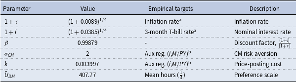
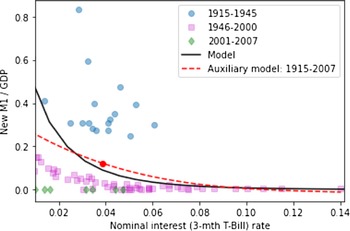
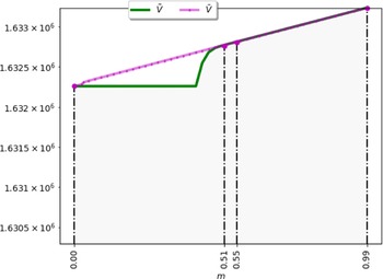

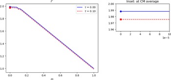


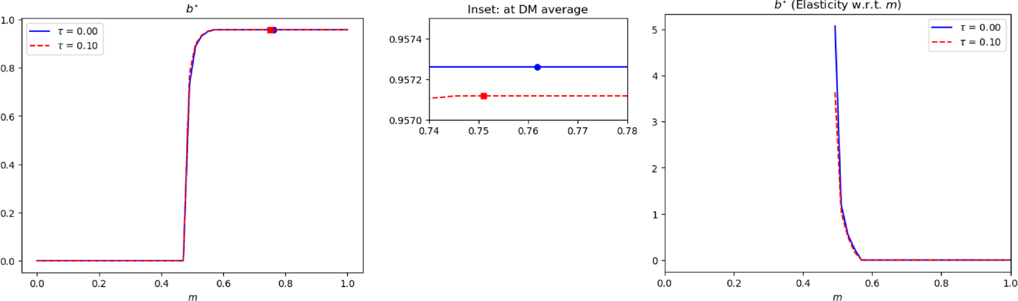


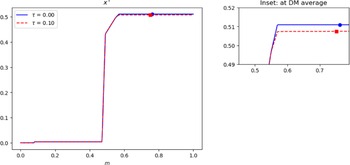


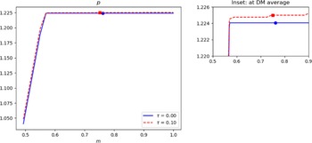

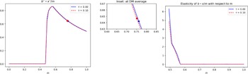


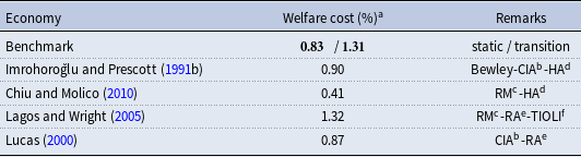
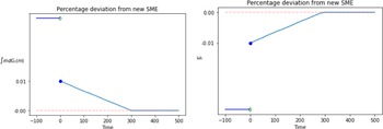


 Open access