


1 Introduction
1.1 Tropical mirror symmetry
Mirror symmetry is a duality between a pair of n-dimensional Calabi-Yau varieties X and $X^{\circ }$
, whereby invariants of the complex geometry of
$X^{\circ }$
, whereby invariants of the complex geometry of $X^{\circ }$
match with invariants of the symplectic geometry of X. There is, by now, a vast literature on mirror symmetry, and the phenomenon can be studied at various levels of depth. A first indication of mirror symmetry is that X and
$X^{\circ }$
match with invariants of the symplectic geometry of X. There is, by now, a vast literature on mirror symmetry, and the phenomenon can be studied at various levels of depth. A first indication of mirror symmetry is that X and $X^{\circ }$
should satisfy the following mirror equality of Hodge numbers:
$X^{\circ }$
should satisfy the following mirror equality of Hodge numbers:
 $$ \begin{align} h^{p,q}(X) = h^{n-p,q}(X^{\circ}). \end{align} $$
Notice that when $p=q=1$
, this equality expresses the fact that the complex deformation space of
$p=q=1$
, this equality expresses the fact that the complex deformation space of $X^{\circ }$
must have the same dimension as the Kähler cone of X. A beautiful construction of mirror pairs of manifolds was discovered by Batyrev [Reference Batyrev5] by considering anti-canonical hypersurfaces in toric varieties associated to dual reflexive polytopes. The construction was later generalized by Borisov [Reference Borisov7] to the case of complete intersections. We point out that in general, the theory is complicated by the fact that in many cases, the Calabi-Yau varieties constructed by this method are singular; therefore, the Hodge numbers in (1) must be replaced by the so-called stringy Hodge numbers. The equality is proved for the hypersurface and complete intersection cases in [Reference Batyrev and Borisov3].
$X^{\circ }$
must have the same dimension as the Kähler cone of X. A beautiful construction of mirror pairs of manifolds was discovered by Batyrev [Reference Batyrev5] by considering anti-canonical hypersurfaces in toric varieties associated to dual reflexive polytopes. The construction was later generalized by Borisov [Reference Borisov7] to the case of complete intersections. We point out that in general, the theory is complicated by the fact that in many cases, the Calabi-Yau varieties constructed by this method are singular; therefore, the Hodge numbers in (1) must be replaced by the so-called stringy Hodge numbers. The equality is proved for the hypersurface and complete intersection cases in [Reference Batyrev and Borisov3].
In this paper, we consider the case of hypersurfaces, assuming that there exists a smooth crepant resolution of both X and $X^{\circ }$
. In this context, our first result is a tropical version of (1). More precisely, if
$X^{\circ }$
. In this context, our first result is a tropical version of (1). More precisely, if $\Delta $
and
$\Delta $
and $\Delta ^{\circ }$
are two dual
$\Delta ^{\circ }$
are two dual $(n+1)$
-dimensional reflexive polytopes, we assume that there exists primitive central subdivisions of both polytopes. These provide resolutions of the ambient toric varieties together with crepant resolutions of the anticanonical hypersurfaces, thus defining a mirror pair of smooth Calabi-Yau varieties X and
$(n+1)$
-dimensional reflexive polytopes, we assume that there exists primitive central subdivisions of both polytopes. These provide resolutions of the ambient toric varieties together with crepant resolutions of the anticanonical hypersurfaces, thus defining a mirror pair of smooth Calabi-Yau varieties X and $X^{\circ }$
. The same data can be used to define the tropical versions of the hypersurfaces
$X^{\circ }$
. The same data can be used to define the tropical versions of the hypersurfaces $X_{\text {trop}}$
and
$X_{\text {trop}}$
and $X_{\text {trop}}^{\circ }$
(see Section 2.3). Itenberg, Katzarkov, Mikhalkin and Zharkov (IKMZ) [Reference Itenberg, Katzarkov, Mikhalkin and Zharkov16] defined the tropical homology groups
$X_{\text {trop}}^{\circ }$
(see Section 2.3). Itenberg, Katzarkov, Mikhalkin and Zharkov (IKMZ) [Reference Itenberg, Katzarkov, Mikhalkin and Zharkov16] defined the tropical homology groups $H_{q}(X_{\text {trop}}; \mathcal F_p)$
for any non-singular tropical variety, as the cellular homology of a certain non-constant cosheaf
$H_{q}(X_{\text {trop}}; \mathcal F_p)$
for any non-singular tropical variety, as the cellular homology of a certain non-constant cosheaf $\mathcal F_p$
of
$\mathcal F_p$
of $\mathbb {Z}$
-modules defined over
$\mathbb {Z}$
-modules defined over $X_{\text {trop}}$
. Our first result is then the following:
$X_{\text {trop}}$
. Our first result is then the following:
Theorem 1.1. Let A be a commutative ring. Given central primitive subdivisions of both $\Delta $
and
$\Delta $
and $\Delta ^{\circ }$
with associated mirror tropical hypersurfaces
$\Delta ^{\circ }$
with associated mirror tropical hypersurfaces $X_{\text {trop}}$
and
$X_{\text {trop}}$
and $X^{\circ }_{\text {trop}}$
, we have canonical isomorphisms
$X^{\circ }_{\text {trop}}$
, we have canonical isomorphisms
 $$\begin{align*}H_{q}(X_{\text{trop}}; \mathcal F_p \otimes A ) \cong H_{q}(X_{\text{trop}}^{\circ}; \mathcal F_{n-p} \otimes A). \end{align*}$$
We believe strongly that one can recover (1) from Theorem 1.1. In fact, the main theorem in [Reference Itenberg, Katzarkov, Mikhalkin and Zharkov16] states in our context that if we can embbed $X_{\text {trop}}$
as a so-called ‘smooth regular
$X_{\text {trop}}$
as a so-called ‘smooth regular $\mathbb {Q}$
-tropical variety’ inside a tropical projective space
$\mathbb {Q}$
-tropical variety’ inside a tropical projective space $\mathbb {T}P^N$
, then
$\mathbb {T}P^N$
, then
 $$ \begin{align} \dim H_{q}(X_{\text{trop}}; \mathcal F_p \otimes \mathbb{Q}) = \dim H^{p,q}(X). \end{align} $$
Unfortunately, it is not clear to us how to prove that such tropical embedding exists. An alternative approach may follow the same line as in [Reference Brugallé, López de Medrano and Rau8], but this is beyond the scope of this paper. This theorem corresponds to Theorem 3.7 and Corollary 3.8, where we state and prove it in a more general combinatorial context. Indeed, using the definition of tropical homology given in [Reference Brugallé, López de Medrano and Rau8], we do not require the subdivision to be convex (i.e., the resolutions of the toric varieties need not be projective). In the convex case and with $A = \mathbb {Q}$
, the mirror relation of Hodge numbers would follow from (2). It is not clear to us what the result means, in the non-convex case, in terms of the Hodge numbers of the corresponding (non-projective) resolutions of the hypersurfaces; see Section 2.2 for details. We also expect that the groups
$A = \mathbb {Q}$
, the mirror relation of Hodge numbers would follow from (2). It is not clear to us what the result means, in the non-convex case, in terms of the Hodge numbers of the corresponding (non-projective) resolutions of the hypersurfaces; see Section 2.2 for details. We also expect that the groups $H_{q}(X_{\text {trop}}; \mathcal F_p \otimes A)$
represent graded pieces of a filtration over the homology (with A coefficients) of the complex hypersurface X, but this has been proved, for any non-singular projective tropical variety, only for
$H_{q}(X_{\text {trop}}; \mathcal F_p \otimes A)$
represent graded pieces of a filtration over the homology (with A coefficients) of the complex hypersurface X, but this has been proved, for any non-singular projective tropical variety, only for $A = \mathbb {Q}$
[Reference Itenberg, Katzarkov, Mikhalkin and Zharkov16]. In particular, when the integral homology of X or
$A = \mathbb {Q}$
[Reference Itenberg, Katzarkov, Mikhalkin and Zharkov16]. In particular, when the integral homology of X or $X^{\circ }$
has torsion, the ranks of these groups with
$X^{\circ }$
has torsion, the ranks of these groups with $A = \mathbb {F}_2$
may differ from the Hodge numbers. In our case, it follows from [Reference Arnal, Renaudineau and Shaw2] that the tropical homology groups have no torsion when the anticanonical bundle is ample (i.e., when
$A = \mathbb {F}_2$
may differ from the Hodge numbers. In our case, it follows from [Reference Arnal, Renaudineau and Shaw2] that the tropical homology groups have no torsion when the anticanonical bundle is ample (i.e., when $\Delta $
is a Delzant polytope). For examples of Calabi-Yau varieties whose integral homology has torsion, see [Reference Batyrev and Kreuzer4]. Another aspect of Theorem 1.1 is that the isomorphism between the tropical homology groups is canonical; however, it is not known whether there exists a canonical isomorphism between the corresponding Hodge groups, except in some special cases (see [Reference Cox and Katz12], Section 4.1.3).
$\Delta $
is a Delzant polytope). For examples of Calabi-Yau varieties whose integral homology has torsion, see [Reference Batyrev and Kreuzer4]. Another aspect of Theorem 1.1 is that the isomorphism between the tropical homology groups is canonical; however, it is not known whether there exists a canonical isomorphism between the corresponding Hodge groups, except in some special cases (see [Reference Cox and Katz12], Section 4.1.3).
The proof of Theorem 1.1 is inspired by the work of Gross-Siebert [Reference Gross and Siebert15] and Yamamoto [Reference Yamamoto23]. For more details, see Section 1.3.
1.2 Patchworking and mirror symmetry
Another implication of mirror symmetry is the expectation that invariants of Lagrangian submanifolds in X are reflected into invariants of coherent sheaves in $X^{\circ }$
. Roughly speaking, this is the content of Kontsevich’s homological mirror symmetry conjecture, which is abstractly formulated into the idea that the derived Fukaya category of Lagrangian submanifolds in X is equivalent to the derived category of coherent sheaves on
$X^{\circ }$
. Roughly speaking, this is the content of Kontsevich’s homological mirror symmetry conjecture, which is abstractly formulated into the idea that the derived Fukaya category of Lagrangian submanifolds in X is equivalent to the derived category of coherent sheaves on $X^{\circ }$
. Given a real Calabi-Yau variety X (i.e., one which is cut out by equations with real coefficients or more generally endowed with an anti-symplectic involution), the real part (or the fixed point set of the involution) is a Lagrangian submanifold. The articles [Reference Castano-Bernard, Matessi and Solomon10], [Reference Argüz and Prince1], [Reference Matessi18] construct and study three-dimensional real Calabi-Yau varieties X where the involution preserves a Lagrangian fibration. Using the Strominger-Yau-Zaslow interpretation of mirror symmetry as a duality between Lagrangian fibrations, a family of real structures on X is parametrized by Lagrangian sections, or equivalently by
$X^{\circ }$
. Given a real Calabi-Yau variety X (i.e., one which is cut out by equations with real coefficients or more generally endowed with an anti-symplectic involution), the real part (or the fixed point set of the involution) is a Lagrangian submanifold. The articles [Reference Castano-Bernard, Matessi and Solomon10], [Reference Argüz and Prince1], [Reference Matessi18] construct and study three-dimensional real Calabi-Yau varieties X where the involution preserves a Lagrangian fibration. Using the Strominger-Yau-Zaslow interpretation of mirror symmetry as a duality between Lagrangian fibrations, a family of real structures on X is parametrized by Lagrangian sections, or equivalently by $\mathbb {F}_2$
-divisor classes D in the mirror
$\mathbb {F}_2$
-divisor classes D in the mirror $X^{\circ }$
[Reference Castano-Bernard, Matessi and Solomon10]. If we denote by
$X^{\circ }$
[Reference Castano-Bernard, Matessi and Solomon10]. If we denote by $\mathbb {R} X_D$
the corresponding real part,
$\mathbb {R} X_D$
the corresponding real part, $\mathbb {R} X_D$
is connected if and only if
$\mathbb {R} X_D$
is connected if and only if $D \neq 0$
. Moreover, the
$D \neq 0$
. Moreover, the $\mathbb {F}_2$
-cohomology of
$\mathbb {F}_2$
-cohomology of $\mathbb {R} X_D$
is determined by the cohomology of the mirror
$\mathbb {R} X_D$
is determined by the cohomology of the mirror $X^{\circ }$
and the homomorphism
$X^{\circ }$
and the homomorphism $\beta : H^2(X^{\circ }, \mathbb {F}_2) \rightarrow H^4(X^{\circ }, \mathbb {F}_2)$
given by
$\beta : H^2(X^{\circ }, \mathbb {F}_2) \rightarrow H^4(X^{\circ }, \mathbb {F}_2)$
given by $\beta (E) = E^2 + DE$
, [Reference Argüz and Prince1], [Reference Matessi18].
$\beta (E) = E^2 + DE$
, [Reference Argüz and Prince1], [Reference Matessi18].
It turns out that the map $\beta $
is a boundary map of a spectral sequence which is similar to the one discovered, in any dimension, by the second author and Shaw [Reference Renaudineau and Shaw20] in the context of real hypersurfaces in toric varieties constructed from primitive patchworking. In the second part of this paper, we study real Calabi-Yau hypersurfaces, of any dimension n, arising from patchworking associated to a primitive central triangulation T of a reflexive polytope
$\beta $
is a boundary map of a spectral sequence which is similar to the one discovered, in any dimension, by the second author and Shaw [Reference Renaudineau and Shaw20] in the context of real hypersurfaces in toric varieties constructed from primitive patchworking. In the second part of this paper, we study real Calabi-Yau hypersurfaces, of any dimension n, arising from patchworking associated to a primitive central triangulation T of a reflexive polytope $\Delta $
. In this case, the sign distribution on the integral points of
$\Delta $
. In this case, the sign distribution on the integral points of $\Delta $
uniquely determines a divisor D in the Picard group, with
$\Delta $
uniquely determines a divisor D in the Picard group, with $\mathbb {F}_2$
coefficients, of the resolved dual toric variety
$\mathbb {F}_2$
coefficients, of the resolved dual toric variety $\mathbb {C} \Sigma _T$
associated to
$\mathbb {C} \Sigma _T$
associated to $\Delta ^{\circ }$
. Indeed, the integral points on the boundary of
$\Delta ^{\circ }$
. Indeed, the integral points on the boundary of $\Delta $
correspond to rays in the fan of
$\Delta $
correspond to rays in the fan of $\mathbb {C} \Sigma _T$
, and therefore to toric divisors. The divisor D is formed by considering the sum of toric divisors whose rays have the same sign as the center of
$\mathbb {C} \Sigma _T$
, and therefore to toric divisors. The divisor D is formed by considering the sum of toric divisors whose rays have the same sign as the center of $\Delta $
(see Figure 5 for a simple example). If we denote by
$\Delta $
(see Figure 5 for a simple example). If we denote by $\mathbb {R} X_D$
the real part of the hypersurface
$\mathbb {R} X_D$
the real part of the hypersurface $X_D$
constructed from patchworking, it turns out (see Proposition 4.1) that if two divisors D and
$X_D$
constructed from patchworking, it turns out (see Proposition 4.1) that if two divisors D and $D'$
are linearly equivalent (over
$D'$
are linearly equivalent (over $\mathbb {F}_2$
), then
$\mathbb {F}_2$
), then $\mathbb {R} X_D$
and
$\mathbb {R} X_D$
and $\mathbb {R} X_{D'}$
are the same up to an automorphism of the ambient toric variety
$\mathbb {R} X_{D'}$
are the same up to an automorphism of the ambient toric variety $\mathbb {C} \Sigma _T$
. Indeed, the signs corresponding to D and
$\mathbb {C} \Sigma _T$
. Indeed, the signs corresponding to D and $D'$
correspond to two octants of the same patchworking.
$D'$
correspond to two octants of the same patchworking.
The main result of the second part is the following.
Theorem 1.2. Let X be a real Calabi-Yau hypersurface arising from a central, primitive patchworking of a reflexive polytope $\Delta $
such that the tropical homology groups
$\Delta $
such that the tropical homology groups $H_{n}(X_{\text {trop}}; \mathcal F_k \otimes \mathbb {F}_2)$
vanish for all
$H_{n}(X_{\text {trop}}; \mathcal F_k \otimes \mathbb {F}_2)$
vanish for all $0 < k < n$
. Then
$0 < k < n$
. Then $\mathbb {R} X_D$
is connected if and only if the tropical divisor class
$\mathbb {R} X_D$
is connected if and only if the tropical divisor class $D_{| X_{\text {trop}}^{\circ }} \in H_{n-1}(X_{\text {trop}}^{\circ }; \mathcal F_{n-1} \otimes \mathbb {F}_2)$
is not zero.
$D_{| X_{\text {trop}}^{\circ }} \in H_{n-1}(X_{\text {trop}}^{\circ }; \mathcal F_{n-1} \otimes \mathbb {F}_2)$
is not zero.
Remark 1.3. We expect that the tropical divisor class $D_{| X_{\text {trop}}^{\circ }}$
vanishes if and only if the complex divisor
$D_{| X_{\text {trop}}^{\circ }}$
vanishes if and only if the complex divisor $D_{|X^{\circ }}$
also vanishes in the
$D_{|X^{\circ }}$
also vanishes in the $\mathbb {F}_2$
-Picard group, but we could not find this result in current literature. We point out that the hypothesis on the vanishing of the tropical homology groups is satisfied, for instance, whenever
$\mathbb {F}_2$
-Picard group, but we could not find this result in current literature. We point out that the hypothesis on the vanishing of the tropical homology groups is satisfied, for instance, whenever $\Delta $
is a Delzant polytope (i.e., when it corresponds to a smooth toric variety with ample anti-canonical bundle [Reference Arnal, Renaudineau and Shaw2], [Reference Brugallé, López de Medrano and Rau8]). Under this hypothesis, the number of connected components of
$\Delta $
is a Delzant polytope (i.e., when it corresponds to a smooth toric variety with ample anti-canonical bundle [Reference Arnal, Renaudineau and Shaw2], [Reference Brugallé, López de Medrano and Rau8]). Under this hypothesis, the number of connected components of $\mathbb {R} X_D$
can be at most two.
$\mathbb {R} X_D$
can be at most two.
The theorem corresponds to Theorem 5.2, where the result is stated in a more general combinatorial context where the subdivision is not assumed to be convex. To prove it, we consider the first page of the spectral sequence in [Reference Renaudineau and Shaw20] converging to the $\mathbb {F}_2$
-homology of the real part
$\mathbb {F}_2$
-homology of the real part $\mathbb {R} X_D$
.
$\mathbb {R} X_D$
.
The part of the spectral sequence which determines the number of connected components starts with the map $\delta ^{[1]}_{D}: H_n( X_{\text {trop}}; \mathcal F_0 \otimes \mathbb {F}_2) \rightarrow H_{n-1}( X_{\text {trop}}; \mathcal F_1 \otimes \mathbb {F}_2)$
. Now
$\delta ^{[1]}_{D}: H_n( X_{\text {trop}}; \mathcal F_0 \otimes \mathbb {F}_2) \rightarrow H_{n-1}( X_{\text {trop}}; \mathcal F_1 \otimes \mathbb {F}_2)$
. Now $H_n( X_{\text {trop}}; \mathcal F_0 \otimes \mathbb {F}_2)$
is one-dimensional and generated by a fundamental class S. It turns out that if we apply the mirror symmetry isomorphism of Theorem 1.1 to the class
$H_n( X_{\text {trop}}; \mathcal F_0 \otimes \mathbb {F}_2)$
is one-dimensional and generated by a fundamental class S. It turns out that if we apply the mirror symmetry isomorphism of Theorem 1.1 to the class $\delta ^{[1]}_{D}(S)$
, we find that it is the tropical divisor class
$\delta ^{[1]}_{D}(S)$
, we find that it is the tropical divisor class $D_{| X_{\text {trop}}^{\circ }} \in H_{n-1}( X_{\text {trop}}^{\circ }; \mathcal F_{n-1} \otimes \mathbb {F}_2)$
. If this class is not zero, then
$D_{| X_{\text {trop}}^{\circ }} \in H_{n-1}( X_{\text {trop}}^{\circ }; \mathcal F_{n-1} \otimes \mathbb {F}_2)$
. If this class is not zero, then $\mathbb {R} X_D$
is connected. If instead it is zero, then we study the maps
$\mathbb {R} X_D$
is connected. If instead it is zero, then we study the maps $\delta ^{[k]}_{D}(S)$
in higher pages of the spectral sequence to show that in this case,
$\delta ^{[k]}_{D}(S)$
in higher pages of the spectral sequence to show that in this case, $\mathbb {R} X_D$
has two connected components.
$\mathbb {R} X_D$
has two connected components.
1.3 Related works
A proof of Theorem 1.1 may also follow by combining the works of Gross-Siebert [Reference Gross and Siebert15] and Gross [Reference Gross14] on mirror symmetry via integral affine manifolds with singularities, with the work of Yamamoto [Reference Yamamoto23]. Indeed, Gross and Siebert associate to a toric degeneration of Calabi-Yau manifolds, an integral affine manifold with singularities (IAMS) (i.e., a topological manifold B with an atlas of integral affine coordinates away from a closed, codimension $2$
subset of B (the dicriminant locus)). The manifold B is the dual intersection complex of the special fibre of the toric degeneration and plays a role similar to the tropical variety
$2$
subset of B (the dicriminant locus)). The manifold B is the dual intersection complex of the special fibre of the toric degeneration and plays a role similar to the tropical variety $X_{\text {trop}}$
. Over B, there are natural sheaves of
$X_{\text {trop}}$
. Over B, there are natural sheaves of $\mathbb {Z}$
-modules, denoted
$\mathbb {Z}$
-modules, denoted $\iota _{\ast } \Lambda ^{\wedge p}$
, where
$\iota _{\ast } \Lambda ^{\wedge p}$
, where $\Lambda $
is a local system induced by the affine coordinates and
$\Lambda $
is a local system induced by the affine coordinates and $\iota $
is the inclusion of the complement of the discriminant locus inside B. The cohomology groups
$\iota $
is the inclusion of the complement of the discriminant locus inside B. The cohomology groups $H^q(B, \iota _{\ast } \Lambda ^{\wedge p})$
play the same role as the tropical homology groups. Two mirror symmetric toric degenerations give dual pairs of integral affine manifolds with singularities B and
$H^q(B, \iota _{\ast } \Lambda ^{\wedge p})$
play the same role as the tropical homology groups. Two mirror symmetric toric degenerations give dual pairs of integral affine manifolds with singularities B and $B^{\circ }$
related to each other by discrete Legendre transform (see Section 1.4 of [Reference Gross and Siebert15]). If
$B^{\circ }$
related to each other by discrete Legendre transform (see Section 1.4 of [Reference Gross and Siebert15]). If $\Lambda ^*$
denotes the dual local system, it is shown that the pairs
$\Lambda ^*$
denotes the dual local system, it is shown that the pairs $(B, \iota _{\ast } \Lambda ^{\wedge p})$
and
$(B, \iota _{\ast } \Lambda ^{\wedge p})$
and $(B^{\circ }, \iota _{\ast } (\Lambda ^*)^{\wedge p})$
are isomorphic (see Proposition 1.50 of [Reference Gross and Siebert15]). However, contraction with a global section of
$(B^{\circ }, \iota _{\ast } (\Lambda ^*)^{\wedge p})$
are isomorphic (see Proposition 1.50 of [Reference Gross and Siebert15]). However, contraction with a global section of $\iota _{\ast } \Lambda ^{\wedge n}$
gives isomorphisms
$\iota _{\ast } \Lambda ^{\wedge n}$
gives isomorphisms $(\Lambda ^*)^{\wedge p} \cong (\Lambda )^{\wedge {n-p}}$
. Thus, we obtain the isomorphism
$(\Lambda ^*)^{\wedge p} \cong (\Lambda )^{\wedge {n-p}}$
. Thus, we obtain the isomorphism $H^q(B, \iota _{\ast } \Lambda ^{\wedge p}) \cong H^q(B^{\circ }, \iota _{\ast } \Lambda ^{\wedge n-p})$
, which is analogous to our Theorem 1.1. In [Reference Gross14], Gross associates to Batyrev-Borisov mirror pairs suitable IAMS and shows they are related by a discrete Legendre transform. The last step is to link the pairs
$H^q(B, \iota _{\ast } \Lambda ^{\wedge p}) \cong H^q(B^{\circ }, \iota _{\ast } \Lambda ^{\wedge n-p})$
, which is analogous to our Theorem 1.1. In [Reference Gross14], Gross associates to Batyrev-Borisov mirror pairs suitable IAMS and shows they are related by a discrete Legendre transform. The last step is to link the pairs $(B, \iota _{\ast } \Lambda ^{\wedge p})$
with
$(B, \iota _{\ast } \Lambda ^{\wedge p})$
with $(X_{\text {trop}}, \mathcal F_p)$
; this is achieved by the work of Yamamoto [Reference Yamamoto23]. Indeed, to the IAMS arising in the Batirev-Borisov construction, Yamamoto associates a tropical variety
$(X_{\text {trop}}, \mathcal F_p)$
; this is achieved by the work of Yamamoto [Reference Yamamoto23]. Indeed, to the IAMS arising in the Batirev-Borisov construction, Yamamoto associates a tropical variety $X_{\text {trop}}$
together with a correspondence between the sheaves.
$X_{\text {trop}}$
together with a correspondence between the sheaves.
Our proof of Theorem 1.1 is inspired by the above works, but it is self-contained, and the isomorphism is more explicit since it is expressed in terms of cellular homology. We define cosheaves $\mathcal M_p$
which are supported on a cellular refinement of the union of the bounded cells of
$\mathcal M_p$
which are supported on a cellular refinement of the union of the bounded cells of $X_{\text {trop}}$
, which is topologically a sphere S. The proof then consists of two steps. First, we show that
$X_{\text {trop}}$
, which is topologically a sphere S. The proof then consists of two steps. First, we show that $\mathcal M_p$
and
$\mathcal M_p$
and $\mathcal F_p$
are linked together by the short exact sequences (17) and (18). These provide the isomorphisms of homology groups
$\mathcal F_p$
are linked together by the short exact sequences (17) and (18). These provide the isomorphisms of homology groups $H^q(X_{\text {trop}}, \mathcal F_p) \cong H^q(S, \mathcal M_p)$
. If
$H^q(X_{\text {trop}}, \mathcal F_p) \cong H^q(S, \mathcal M_p)$
. If $S^{\circ }$
is the sphere associated to
$S^{\circ }$
is the sphere associated to $X_{\text {trop}}^{\circ }$
, the next step is to define a cellular isomorphism between S and
$X_{\text {trop}}^{\circ }$
, the next step is to define a cellular isomorphism between S and $S^\circ $
such that the pairs
$S^\circ $
such that the pairs $(S, \mathcal M_p)$
and
$(S, \mathcal M_p)$
and $(S^{\circ }, \mathcal M_{n-p})$
are isomorphic. The two steps are the content of Theorem 3.7, and together they give the isomorphism in Theorem 1.1. Notice that the pairs
$(S^{\circ }, \mathcal M_{n-p})$
are isomorphic. The two steps are the content of Theorem 3.7, and together they give the isomorphism in Theorem 1.1. Notice that the pairs $(S, \mathcal M_p)$
should be isomorphic to the pairs
$(S, \mathcal M_p)$
should be isomorphic to the pairs $(B, \iota _{\ast } \Lambda ^{\wedge p})$
from the work of Gross-Siebert.
$(B, \iota _{\ast } \Lambda ^{\wedge p})$
from the work of Gross-Siebert.
Our approach is also inspired by the work [Reference Brugallé, López de Medrano and Rau8] where the authors define tropical homology groups also in the case of non-convex primitive subdivisions, where there is no associated tropical variety. They also extend to this setting the definition of real phase structures from [Reference Renaudineau and Shaw20], together with the spectral sequence computing the cohomology of the real part.
1.4 Outlook
To prove Theorem 1.2, we explicitly compute the boundary map $\delta ^{[1]}_{D}: H_n( X_{\text {trop}}; \mathcal F_0 \otimes \mathbb {F}_2) \rightarrow H_{n-1}( X_{\text {trop}}; \mathcal F_1 \otimes \mathbb {F}_2)$
of the spectral sequence from [Reference Renaudineau and Shaw20] and then apply the mirror symmetry isomorphism of Theorem 1.1. More generally, we have the other boundary maps
$\delta ^{[1]}_{D}: H_n( X_{\text {trop}}; \mathcal F_0 \otimes \mathbb {F}_2) \rightarrow H_{n-1}( X_{\text {trop}}; \mathcal F_1 \otimes \mathbb {F}_2)$
of the spectral sequence from [Reference Renaudineau and Shaw20] and then apply the mirror symmetry isomorphism of Theorem 1.1. More generally, we have the other boundary maps
 $$\begin{align*}\delta^{[1]}_{D}: H_q( X_{\text{trop}}; \mathcal F_p \otimes \mathbb{F}_2) \rightarrow H_{q-1}( X_{\text{trop}}; \mathcal F_{p+1} \otimes \mathbb{F}_2). \end{align*}$$
If we compose with the mirror isomorphisms, we get maps on the tropical homology of the mirror
 $$\begin{align*}\delta^{[1]}_{D}: H_q( X^{\circ}_{\text{trop}}; \mathcal F_p \otimes \mathbb{F}_2) \rightarrow H_{q-1}( X^{\circ}_{\text{trop}}; \mathcal F_{p-1} \otimes \mathbb{F}_2). \end{align*}$$
We expect that these maps have a geometric description involving the divisor class D and standard operations on (co)-homology (such as intersection products), similar to the maps found in [Reference Argüz and Prince1], [Reference Matessi18]. We are confident that the explicit description of the mirror symmetry isomorphism given in proof of Theorem 1.1 is suitably adapted to do this computation.
2 Toric, tropical and combinatorial geometry
In this section, we review some background material on toric and tropical geometry. Some references are [Reference Fulton13], [Reference Cox, Little and Schenck11], [Reference Batyrev5], [Reference Cox and Katz12] for toric geometry; [Reference Brugallé, Itenberg, Mikhalkin and Shaw9], [Reference Mikhalkin and Rau19] for tropical geometry; and [Reference Itenberg, Katzarkov, Mikhalkin and Zharkov16], [Reference Brugallé, López de Medrano and Rau8] for tropical homology.
2.1 Polytopes and toric varieties
Let $M \cong \mathbb {Z}^{n+1}$
be a lattice and let
$M \cong \mathbb {Z}^{n+1}$
be a lattice and let $N = \operatorname {\mathrm {Hom}}(M, \mathbb {Z})$
be its dual lattice. We define
$N = \operatorname {\mathrm {Hom}}(M, \mathbb {Z})$
be its dual lattice. We define $M_{\mathbb {R}} = M \otimes \mathbb {R}$
and
$M_{\mathbb {R}} = M \otimes \mathbb {R}$
and $N_{\mathbb {R}} = N \otimes \mathbb {R}$
. A lattice polytope
$N_{\mathbb {R}} = N \otimes \mathbb {R}$
. A lattice polytope $\Delta $
in
$\Delta $
in $M_{\mathbb {R}}$
is the convex hull of a finite number of points of M. In this paper, we will always assume that
$M_{\mathbb {R}}$
is the convex hull of a finite number of points of M. In this paper, we will always assume that $\Delta $
is full dimensional. We will denote by greek letters (
$\Delta $
is full dimensional. We will denote by greek letters ( $\sigma $
,
$\sigma $
, $\tau $
, etc.) the faces of
$\tau $
, etc.) the faces of $\Delta $
. The normal fan
$\Delta $
. The normal fan $\Sigma _{\Delta }$
of
$\Sigma _{\Delta }$
of $\Delta $
is the collection of convex rational cones
$\Delta $
is the collection of convex rational cones $\{ C_{\sigma }\}_{\sigma \preceq \Delta }$
in
$\{ C_{\sigma }\}_{\sigma \preceq \Delta }$
in $N_{\mathbb {R}}$
given by
$N_{\mathbb {R}}$
given by
 $$\begin{align*}C_{\sigma} = \{ v \in N_{\mathbb{R}} \, | \, \langle {v}, {w-u} \rangle \geq 0, \quad \forall u \in \sigma \ \text{and} \ w \in \Delta \}. \end{align*}$$
We will work with complex, real and tropical toric varieties. Let us briefly recall how they are constructed. Let $\Sigma $
be a rational strongly convex polyhedral fan in
$\Sigma $
be a rational strongly convex polyhedral fan in $N_{\mathbb {R}}$
. For any cone
$N_{\mathbb {R}}$
. For any cone $\sigma $
of
$\sigma $
of $\Sigma $
, consider the dual cone
$\Sigma $
, consider the dual cone
 $$ \begin{align*}\sigma^{\vee} = \{ u \in M_{\mathbb{R}} \, | \, \langle {u}, {v} \rangle \geq 0, \quad \forall v \in \sigma\}. \end{align*} $$
By Gordon’s Lemma, the intersection $S_\sigma =\sigma ^{\vee }\cap M$
is a finitely generated semigroup. So for any semigroup S, one can consider the set
$S_\sigma =\sigma ^{\vee }\cap M$
is a finitely generated semigroup. So for any semigroup S, one can consider the set $X_\sigma ^S:=\operatorname {\mathrm {Hom}}(S_\sigma ,S)$
of semigroup homomorphisms. If moreover the semigroup S has a topology, we equipp the set
$X_\sigma ^S:=\operatorname {\mathrm {Hom}}(S_\sigma ,S)$
of semigroup homomorphisms. If moreover the semigroup S has a topology, we equipp the set $X_\sigma ^S$
with the coarsest topology such that for any
$X_\sigma ^S$
with the coarsest topology such that for any $\lambda \in S_\sigma $
, the corresponding evaluation map
$\lambda \in S_\sigma $
, the corresponding evaluation map $X_\sigma ^S\rightarrow S$
is continuous. In fact, it is enough to do it for a set of generators of
$X_\sigma ^S\rightarrow S$
is continuous. In fact, it is enough to do it for a set of generators of $S_\sigma $
(say of cardinality N), and the topology coincides with the induced topology from
$S_\sigma $
(say of cardinality N), and the topology coincides with the induced topology from $S^N$
. If
$S^N$
. If $\sigma \subset \tau $
, there is a continuous restriction map from
$\sigma \subset \tau $
, there is a continuous restriction map from $X_\sigma ^S$
to
$X_\sigma ^S$
to $X_\tau ^S$
.
$X_\tau ^S$
.
Definition 2.1. The toric variety associated to the fan $\Sigma $
over the semigroup S is the direct limit
$\Sigma $
over the semigroup S is the direct limit
 $$ \begin{align*}S\Sigma := \varinjlim X_\sigma^S. \end{align*} $$
Classically, the most common semigroups are either $\mathbb {R}$
,
$\mathbb {R}$
, $\mathbb {C}$
or
$\mathbb {C}$
or $\mathbb {R}_+$
(for multiplication). We will also consider the tropical semigroup
$\mathbb {R}_+$
(for multiplication). We will also consider the tropical semigroup $\mathbb {T}:=\mathbb {R}\cup {-\infty }$
with the tropical multiplication being the addition. The neutral element
$\mathbb {T}:=\mathbb {R}\cup {-\infty }$
with the tropical multiplication being the addition. The neutral element $1_{\mathbb {T}}$
is equal to
$1_{\mathbb {T}}$
is equal to $0$
, while the zero element
$0$
, while the zero element $0_{\mathbb {T}}$
is
$0_{\mathbb {T}}$
is $-\infty $
. All these semigroups are equipped with the euclidean topology. The torus
$-\infty $
. All these semigroups are equipped with the euclidean topology. The torus $N\otimes S^*$
is open in
$N\otimes S^*$
is open in $S\Sigma $
and acts on each
$S\Sigma $
and acts on each $X^S_\sigma $
, and this action extends to all of
$X^S_\sigma $
, and this action extends to all of $S\Sigma $
. The orbits are in correspondence with the cones of
$S\Sigma $
. The orbits are in correspondence with the cones of $\Sigma $
via the map
$\Sigma $
via the map $\sigma \rightarrow \mathcal {O}^S_\sigma $
, where
$\sigma \rightarrow \mathcal {O}^S_\sigma $
, where $\mathcal {O}^S_\sigma $
is the orbit of the point
$\mathcal {O}^S_\sigma $
is the orbit of the point $x_\sigma \in X^S_\sigma $
defined by
$x_\sigma \in X^S_\sigma $
defined by
 $$ \begin{align*}x_\sigma(m)=\left\lbrace \begin{array}{@{}c} 1_S \text{ if } -m\in S_\sigma, \\ 0_S \text{ otherwise }.\end{array}\right.\end{align*} $$
For $S=\mathbb {C}$
, we obtain the classical construction of complex toric varieties; see Section 1.3 of [Reference Fulton13]. If
$S=\mathbb {C}$
, we obtain the classical construction of complex toric varieties; see Section 1.3 of [Reference Fulton13]. If $\Sigma =\Sigma _\Delta $
is the normal fan of a lattice polytope, the variety
$\Sigma =\Sigma _\Delta $
is the normal fan of a lattice polytope, the variety $\mathbb {C}\Sigma $
is projective. A fan
$\mathbb {C}\Sigma $
is projective. A fan $\Sigma $
is said to be regular if every cone can be generated by a subset of a basis of N. Then the toric variety
$\Sigma $
is said to be regular if every cone can be generated by a subset of a basis of N. Then the toric variety $\mathbb {C}\Sigma $
is smooth if and only if
$\mathbb {C}\Sigma $
is smooth if and only if $\Sigma $
is regular. A polytope in
$\Sigma $
is regular. A polytope in $M_{\mathbb {R}}$
is called non-singular if its normal fan is regular. We say
$M_{\mathbb {R}}$
is called non-singular if its normal fan is regular. We say $\Sigma $
is complete if its support
$\Sigma $
is complete if its support $|\Sigma |$
(i.e., the union of its cones) is equal to
$|\Sigma |$
(i.e., the union of its cones) is equal to $N_{\mathbb {R}}$
. Completeness is necessary and sufficient for the toric variety
$N_{\mathbb {R}}$
. Completeness is necessary and sufficient for the toric variety $\mathbb {C} \Sigma $
to be compact. For any fan
$\mathbb {C} \Sigma $
to be compact. For any fan $\Sigma $
, there is a natural map from
$\Sigma $
, there is a natural map from $\mathbb {C}\Sigma $
to
$\mathbb {C}\Sigma $
to $\mathbb {R}_+\Sigma $
induced by the absolute value from
$\mathbb {R}_+\Sigma $
induced by the absolute value from $\mathbb {C}$
to
$\mathbb {C}$
to $\mathbb {R}_+$
(composition with the logarithm will identify
$\mathbb {R}_+$
(composition with the logarithm will identify $\mathbb {R}_+\Sigma $
with
$\mathbb {R}_+\Sigma $
with $\mathbb {T}\Sigma $
). In the case where
$\mathbb {T}\Sigma $
). In the case where $\Sigma =\Sigma _\Delta $
, one has
$\Sigma =\Sigma _\Delta $
, one has $\mathbb {R}_+\Sigma _{\Delta }=\Delta $
, and the map
$\mathbb {R}_+\Sigma _{\Delta }=\Delta $
, and the map $\mathbb {C}\Sigma _{\Delta }$
to
$\mathbb {C}\Sigma _{\Delta }$
to $\Delta $
is the moment map. In general, the real toric variety
$\Delta $
is the moment map. In general, the real toric variety $\mathbb {R} \Sigma $
can be reconstructed combinatorially directly form the fan
$\mathbb {R} \Sigma $
can be reconstructed combinatorially directly form the fan $\Sigma $
as follows (see, for example, [Reference Bihan, Franz, McCrory and van Bihan6]). For any group homomorphism
$\Sigma $
as follows (see, for example, [Reference Bihan, Franz, McCrory and van Bihan6]). For any group homomorphism $\xi :M\rightarrow \mathbb {F}_2$
, consider
$\xi :M\rightarrow \mathbb {F}_2$
, consider $\mathbb {R}_+\Sigma (\xi )$
a copy of
$\mathbb {R}_+\Sigma (\xi )$
a copy of $\mathbb {R}_+\Sigma $
. Then
$\mathbb {R}_+\Sigma $
. Then
 $$ \begin{align} \mathbb{R} \Sigma\simeq \bigsqcup_{\xi\in \operatorname{\mathrm{Hom}}(M,\mathbb{F}_2)}\mathbb{R}_+\Sigma(\xi) / \sim, \end{align} $$
where $(p,\xi )\sim (p',\xi ')$
if and only if
$(p,\xi )\sim (p',\xi ')$
if and only if $p=p'$
and
$p=p'$
and $\xi \vert _{\sigma ^{\perp }}=\xi '\vert _{\sigma ^{\perp }}$
for the unique cone
$\xi \vert _{\sigma ^{\perp }}=\xi '\vert _{\sigma ^{\perp }}$
for the unique cone $\sigma $
such that
$\sigma $
such that $p\in \mathcal {O}^{\mathbb {R}_+}_\sigma $
.
$p\in \mathcal {O}^{\mathbb {R}_+}_\sigma $
.
2.2 Reflexive polytopes and mirror symmetry
A lattice polytope $\Delta $
is called reflexive if it is defined by a system of inequalities
$\Delta $
is called reflexive if it is defined by a system of inequalities $ \langle {v}, {u} \rangle \leq 1$
with
$ \langle {v}, {u} \rangle \leq 1$
with $v\in N$
and
$v\in N$
and $u\in M_{\mathbb {R}}$
. In particular, it implies that
$u\in M_{\mathbb {R}}$
. In particular, it implies that $\operatorname {\mathrm {Int}}(\Delta ) \cap M = \{ 0 \}$
(i.e.,
$\operatorname {\mathrm {Int}}(\Delta ) \cap M = \{ 0 \}$
(i.e., $0$
is the unique interior lattice point of
$0$
is the unique interior lattice point of $\Delta $
). The dual polytope
$\Delta $
). The dual polytope $ \Delta ^{\circ } \subset N_{\mathbb {R}}$
is defined as
$ \Delta ^{\circ } \subset N_{\mathbb {R}}$
is defined as
 $$\begin{align*}\Delta^{\circ} = \{ u \in N_{\mathbb{R}} \, | \, \langle {u}, {v} \rangle \leq 1, \quad \forall v \in \Delta \}. \end{align*}$$
If $\Delta $
is reflexive, then
$\Delta $
is reflexive, then $\Delta ^{\circ }$
is a lattice polytope which is also reflexive and
$\Delta ^{\circ }$
is a lattice polytope which is also reflexive and $(\Delta ^{\circ })^\circ = \Delta $
.
$(\Delta ^{\circ })^\circ = \Delta $
.
A reflexive polytope $\Delta \subset M_{\mathbb {R}}$
defines another fan, in the same space
$\Delta \subset M_{\mathbb {R}}$
defines another fan, in the same space $M_{\mathbb {R}}$
called the face fan of
$M_{\mathbb {R}}$
called the face fan of $\Delta $
denoted by
$\Delta $
denoted by $\Xi _{\Delta }$
whose cones are the cones over the faces of
$\Xi _{\Delta }$
whose cones are the cones over the faces of $\Delta $
. We have the following relations:
$\Delta $
. We have the following relations:
 $$\begin{align*}\Xi_{\Delta} = \Sigma_{\Delta^{\circ}} \quad \text{and} \quad \Xi_{\Delta^{\circ}} = \Sigma_{\Delta}.\end{align*}$$
Definition 2.2. A lattice simplex is called primitive (sometimes also unimodular) if its volume is $\frac {1}{(n+1)!}$
, the minimal possible volume among lattice simplices.
$\frac {1}{(n+1)!}$
, the minimal possible volume among lattice simplices.
If $\Delta $
is a non-singular reflexive polytope, then the cones of
$\Delta $
is a non-singular reflexive polytope, then the cones of $\Xi _{\Delta ^{\circ }}$
are regular. So all faces of
$\Xi _{\Delta ^{\circ }}$
are regular. So all faces of $\Delta ^{\circ }$
are simplices with no integer points in the interior. Moreover, if
$\Delta ^{\circ }$
are simplices with no integer points in the interior. Moreover, if $\sigma $
is a facet of
$\sigma $
is a facet of $\Delta ^{\circ }$
, then the convex hull of the origin in N with
$\Delta ^{\circ }$
, then the convex hull of the origin in N with $\sigma $
is a primitive simplex.
$\sigma $
is a primitive simplex.
Given a pair of dual polytopes $\Delta $
and
$\Delta $
and $\Delta ^{\circ }$
, we can consider anticanonical subvarieties X and
$\Delta ^{\circ }$
, we can consider anticanonical subvarieties X and $X^{\circ }$
inside
$X^{\circ }$
inside $\mathbb {C}\Sigma _{\Delta }$
and
$\mathbb {C}\Sigma _{\Delta }$
and $\mathbb {C}\Sigma _{\Delta ^{\circ }}$
, respectively. These are both Calabi-Yau varieties, and they constitute a so called mirror pair. Typically these varieties, as well as the ambient toric varieties, will be singular. Sometimes singularities can be resolved in the realm of Calabi-Yau varieties by a crepant resolution. The easiest way to do this, if possible, is to consider primitive convex central subdivisions.
$\mathbb {C}\Sigma _{\Delta ^{\circ }}$
, respectively. These are both Calabi-Yau varieties, and they constitute a so called mirror pair. Typically these varieties, as well as the ambient toric varieties, will be singular. Sometimes singularities can be resolved in the realm of Calabi-Yau varieties by a crepant resolution. The easiest way to do this, if possible, is to consider primitive convex central subdivisions.
Definition 2.3. Let $\Delta \subset M_{\mathbb {R}}$
be a reflexive polytope. A triangulation of
$\Delta \subset M_{\mathbb {R}}$
be a reflexive polytope. A triangulation of $\Delta $
with vertices in M is called central if it is obtained by taking convex hulls of the origin in M and any element of a triangulation of the facets of
$\Delta $
with vertices in M is called central if it is obtained by taking convex hulls of the origin in M and any element of a triangulation of the facets of $\Delta $
. We say that the subdivision is convex if it is induced by an integral convex piecewise linear function on
$\Delta $
. We say that the subdivision is convex if it is induced by an integral convex piecewise linear function on $\Delta $
. The triangulation is primitive if all of its elements are primitive simplices. We will also denote by T a triangulation and by
$\Delta $
. The triangulation is primitive if all of its elements are primitive simplices. We will also denote by T a triangulation and by $\partial T$
the simplices of T which are contained in the boundary
$\partial T$
the simplices of T which are contained in the boundary $\partial \Delta $
.
$\partial \Delta $
.
Let T be a primitive central triangulation of $\Delta $
. Denote by
$\Delta $
. Denote by $\Sigma _T$
the regular fan constructed by taking the cones from the origin of M over the simplices in the subdivision of
$\Sigma _T$
the regular fan constructed by taking the cones from the origin of M over the simplices in the subdivision of $\Delta $
. This fan is a refinement of the fan
$\Delta $
. This fan is a refinement of the fan $\Xi _{\Delta }=\Sigma _{\Delta ^{\circ }}$
. So it defines a desingularization
$\Xi _{\Delta }=\Sigma _{\Delta ^{\circ }}$
. So it defines a desingularization $ \mathbb {C}\Sigma _{T}$
of
$ \mathbb {C}\Sigma _{T}$
of $\mathbb {C}\Sigma _{\Delta ^{\circ }}$
.
$\mathbb {C}\Sigma _{\Delta ^{\circ }}$
.
In this article, we assume there exist primitive triangulations T and $T^{\circ }$
of
$T^{\circ }$
of $\Delta $
and
$\Delta $
and $\Delta ^{\circ }$
, respectively, we do not always assume they are convex. In this case, generic anti-canonical hypersurfaces in
$\Delta ^{\circ }$
, respectively, we do not always assume they are convex. In this case, generic anti-canonical hypersurfaces in $\mathbb {C}\Sigma _{T^{\circ }}$
or
$\mathbb {C}\Sigma _{T^{\circ }}$
or $\mathbb {C}\Sigma _{T}$
are smooth Calabi-Yau varieties. From now on, we will denote by X and
$\mathbb {C}\Sigma _{T}$
are smooth Calabi-Yau varieties. From now on, we will denote by X and $X^{\circ }$
smooth anticanonical hypersurfaces in
$X^{\circ }$
smooth anticanonical hypersurfaces in $\mathbb {C}\Sigma _{T^{\circ }}$
and
$\mathbb {C}\Sigma _{T^{\circ }}$
and $\mathbb {C}\Sigma _{T}$
, respectively, instead of the singular ones in
$\mathbb {C}\Sigma _{T}$
, respectively, instead of the singular ones in $\mathbb {C}\Sigma _{\Delta }$
and
$\mathbb {C}\Sigma _{\Delta }$
and $\mathbb {C}\Sigma _{\Delta ^{\circ }}$
. When the triangulations are not convex, these may be non-projective. In the projective case (i.e., when T and
$\mathbb {C}\Sigma _{\Delta ^{\circ }}$
. When the triangulations are not convex, these may be non-projective. In the projective case (i.e., when T and $T^{\circ }$
are both convex), Batyrev and Borisov [Reference Batyrev and Borisov3] proved that the Hodge numbers of X and
$T^{\circ }$
are both convex), Batyrev and Borisov [Reference Batyrev and Borisov3] proved that the Hodge numbers of X and $X^{\circ }$
satisfy the following mirror identity (see also [Reference Cox and Katz12]):
$X^{\circ }$
satisfy the following mirror identity (see also [Reference Cox and Katz12]):
 $$\begin{align*}h^{p,q}(X) = h^{n-p,q}(X^{\circ}). \end{align*}$$
This relation is in fact proved in Theorem 4.15 of [Reference Batyrev and Borisov3] in the case where the Hodge numbers are replaced by the so called stringy-Hodge numbers, which only depend on the singular Calabi-Yau. Then, Proposition 1.1 of [Reference Batyrev and Borisov3] states that the stringy Hodge numbers coincide with the Hodge numbers of the smooth, projective crepant resolutions given by T and $T^{\circ }$
. We expect that the mirror identity of Hodge numbers should also hold in the non-projective case, although we could not find a proof of this in the literature.
$T^{\circ }$
. We expect that the mirror identity of Hodge numbers should also hold in the non-projective case, although we could not find a proof of this in the literature.
2.3 Combinatorial mirror pairs
Let us introduce first some important notations we will use all along the paper. Given a simplex $\sigma \in T$
,
$\sigma \in T$
,
-
• denote by $C(\sigma ) \in \Sigma _{T}$
the cone over
$\sigma $
;
$C(\sigma ) \in \Sigma _{T}$
the cone over
$\sigma $
; -
• denote by
$\sigma ^{\perp }$
the subspace of N orthogonal to the integral tangent space of
$\sigma $
; -
• if
$\sigma \neq 0$
, let
$$ \begin{align*}\sigma_{\infty} = \sigma \cap \partial \Delta.\end{align*} $$


Given a cone $\rho \in \Sigma _{T}$
,
$\rho \in \Sigma _{T}$
,
-
• denote by
$S(\rho )$
the simplex
$\rho \cap \Delta $
; -
• denote by
$\hat {\sigma }$
the simplex
$S(C(\sigma ))$
(i.e., the convex hull of
$0$
and
$\sigma $
).


In particular, when $0 \in \sigma $
, then
$0 \in \sigma $
, then $\hat {\sigma }=\sigma $
and
$\hat {\sigma }=\sigma $
and $\sigma _{\infty }$
is the unique facet of
$\sigma _{\infty }$
is the unique facet of $\sigma $
contained in
$\sigma $
contained in $\partial \Delta $
. If
$\partial \Delta $
. If $0 \notin \sigma $
, then
$0 \notin \sigma $
, then $\sigma _{\infty } = \sigma $
.
$\sigma _{\infty } = \sigma $
.
Given two fans $\Sigma $
and
$\Sigma $
and $\Sigma '$
such that
$\Sigma '$
such that $\Sigma $
is a refinement of
$\Sigma $
is a refinement of $\Sigma '$
,
$\Sigma '$
,
-
• for every cone
$\rho \in \Sigma $
, denote by
$\min (\rho )$
the smallest cone of
$\Sigma '$
containing
$\rho $
.


If $\Sigma $
is the normal fan of a polytope
$\Sigma $
is the normal fan of a polytope $\Delta $
,
$\Delta $
,
-
• denote by
$\rho ^{\vee }$
the face of
$\Delta $
which is normal to
$\rho $
, and by
$F^\vee $
the cone of
$\Sigma $
which is normal to the face F of
$\Delta $
.


Assume for a moment that T is a primitive convex central triangulation of $\Delta $
. If
$\Delta $
. If ${\mu :\Delta \cap M\rightarrow \mathbb {Z}_{\geq 0}}$
is a convex function ensuring the convexity of T, one can consider its Legendre transform (defined over
${\mu :\Delta \cap M\rightarrow \mathbb {Z}_{\geq 0}}$
is a convex function ensuring the convexity of T, one can consider its Legendre transform (defined over $N_{\mathbb {R}}$
):
$N_{\mathbb {R}}$
):
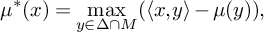 $$ \begin{align} \mu^*(x)=\max_{y\in\Delta\cap M} ( \langle x,y\rangle -\mu(y)), \end{align} $$
and the set
 $$ \begin{align*}V_\mu:=\left\lbrace x\in N_{\mathbb{R}} \mid \exists y_1\neq y_2, \:\: \mu^*(x) = \langle x,y_1\rangle -\mu(y_1)=\langle x,y_2\rangle -\mu(y_2)\right\rbrace. \end{align*} $$
In other words, the set $V_\mu $
is the set of points where the maximum in (4) is attained at least twice. It is the so-called tropical hypersurface associated to
$V_\mu $
is the set of points where the maximum in (4) is attained at least twice. It is the so-called tropical hypersurface associated to $\mu $
: it is a weighted rational balanced polyhedral complex, inducing a polyhedral subdivision of
$\mu $
: it is a weighted rational balanced polyhedral complex, inducing a polyhedral subdivision of $N_{\mathbb {R}}$
which is dual (as a poset) to the triangulation T (see, for example, [Reference Brugallé, Itenberg, Mikhalkin and Shaw9] for more details). Moreover, the compactification of
$N_{\mathbb {R}}$
which is dual (as a poset) to the triangulation T (see, for example, [Reference Brugallé, Itenberg, Mikhalkin and Shaw9] for more details). Moreover, the compactification of $V_\mu $
in the tropical toric variety
$V_\mu $
in the tropical toric variety $\mathbb {T}\Sigma _\Delta $
induces a subdivision of
$\mathbb {T}\Sigma _\Delta $
induces a subdivision of $\mathbb {T}\Sigma _\Delta $
with underlying poset the subposet of
$\mathbb {T}\Sigma _\Delta $
with underlying poset the subposet of $\Sigma _\Delta \times T$
:
$\Sigma _\Delta \times T$
:
 $$ \begin{align} \Phi:=\left\lbrace (\rho,\sigma)\in\Sigma_\Delta\times T \mid \sigma\subset \rho^\vee \right\rbrace. \end{align} $$
The order on the poset is the inverse of the inclusion, meaning that $(\rho ,\sigma )\leq (\rho ',\sigma ')$
iff
$(\rho ,\sigma )\leq (\rho ',\sigma ')$
iff $\rho '\subset \rho $
and
$\rho '\subset \rho $
and $\sigma '\subset \sigma $
(see [Reference Brugallé, López de Medrano and Rau8] Remark 2.3).
$\sigma '\subset \sigma $
(see [Reference Brugallé, López de Medrano and Rau8] Remark 2.3).
Definition 2.4. Let T be an primitive convex central triangulation of $\Delta $
and
$\Delta $
and $T^\circ $
be a primitive convex central triangulation of
$T^\circ $
be a primitive convex central triangulation of $\Delta ^\circ $
, induced respectively by convex functions
$\Delta ^\circ $
, induced respectively by convex functions $\mu $
and
$\mu $
and $\mu ^\circ $
. We denote by
$\mu ^\circ $
. We denote by $X_{\text {trop}}$
the compactification of
$X_{\text {trop}}$
the compactification of $V_\mu $
inside
$V_\mu $
inside $\mathbb {T}\Sigma _{T^\circ }$
and by
$\mathbb {T}\Sigma _{T^\circ }$
and by $X_{\text {trop}}^\circ $
the compactification of
$X_{\text {trop}}^\circ $
the compactification of $V_{\mu ^\circ }$
inside
$V_{\mu ^\circ }$
inside $\mathbb {T}\Sigma _{T}$
.
$\mathbb {T}\Sigma _{T}$
.
The tropical variety $X_{\text {trop}}$
induces a subdivision of
$X_{\text {trop}}$
induces a subdivision of $\mathbb {T}\Sigma _{T^\circ }$
with underlying poset the subposet of
$\mathbb {T}\Sigma _{T^\circ }$
with underlying poset the subposet of $T^\circ \times T$
defined by
$T^\circ \times T$
defined by
 $$ \begin{align*}\mathcal{P}(T^\circ,T):=\left\lbrace (\tau,\sigma)\in T^\circ\times T \: \mid \: 0\in\tau \text{ and } \sigma\subset \min(C(\tau))^\vee \right\rbrace .\end{align*} $$
Recall that $C(\tau )$
is the cone (in
$C(\tau )$
is the cone (in $\Sigma _{T^\circ }$
) over
$\Sigma _{T^\circ }$
) over $\tau $
. The fan
$\tau $
. The fan $\Sigma _{T^\circ }$
is a refinement of the fan
$\Sigma _{T^\circ }$
is a refinement of the fan $\Xi _{\Delta ^\circ }$
, which is the normal fan of
$\Xi _{\Delta ^\circ }$
, which is the normal fan of $\Delta $
. Then by definition,
$\Delta $
. Then by definition, $\min (C(\tau ))^\vee $
is a face of
$\min (C(\tau ))^\vee $
is a face of $\Delta $
. The order on the poset
$\Delta $
. The order on the poset $\mathcal {P}(T^\circ ,T)$
is also the inverse of the inclusion.
$\mathcal {P}(T^\circ ,T)$
is also the inverse of the inclusion.
Example 2.5. Let
 $$\begin{align*}\Delta = \operatorname{\mathrm{Conv}}((-1,-1), \ (-1,2), \ (2,-1)). \end{align*}$$
It is a reflexive polygon, and its dual is given by
 $$\begin{align*}\Delta^\circ = \operatorname{\mathrm{Conv}}((1,1), (-1,0),(0,-1)).\end{align*}$$
Denote by T and $T^\circ $
their unique primitive central triangulations. They are both convex. We draw in Figure 1 the subdivision of
$T^\circ $
their unique primitive central triangulations. They are both convex. We draw in Figure 1 the subdivision of $\mathbb {T}\Sigma _{T^\circ }$
induced by a tropical curve dual to T and some examples of cells in the underlying poset
$\mathbb {T}\Sigma _{T^\circ }$
induced by a tropical curve dual to T and some examples of cells in the underlying poset $\mathcal {P}(T^\circ ,T)$
.
$\mathcal {P}(T^\circ ,T)$
.
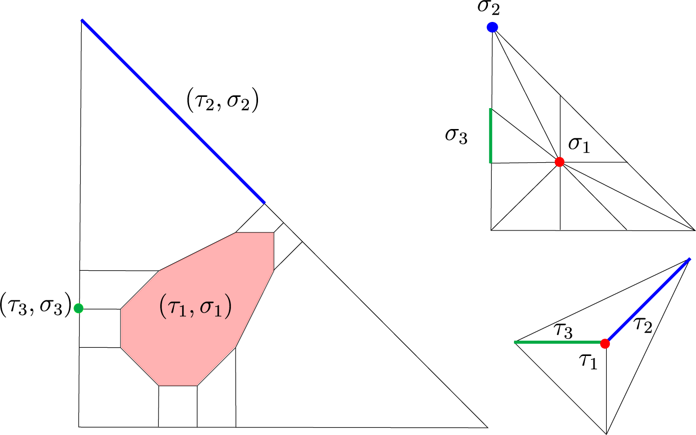
Figure 1 The subdivision of $\mathbb {T}\Sigma _{T^\circ }$
induced by a tropical curve dual to T.
$\mathbb {T}\Sigma _{T^\circ }$
induced by a tropical curve dual to T.
In fact, in this paper, we do not assume any convexity hypothesis. For any T and $T^\circ $
as above (not necessarily convex), one can still consider the posets
$T^\circ $
as above (not necessarily convex), one can still consider the posets $\mathcal {P}(T,T^{\circ })$
and
$\mathcal {P}(T,T^{\circ })$
and $\mathcal {P}(T^{\circ },T)$
. Recall that to any poset P is associated an abstract simplicial complex, called the order complex, whose vertices are the elements of P and whose simplices are the (finite) nonempty chains of P. Moreover, to any simplicial complex, there is a topological space called the geometric realization defined by formal convex combinations of vertices belonging to a simplex. The geometric realization of a poset P will be denoted by
$\mathcal {P}(T^{\circ },T)$
. Recall that to any poset P is associated an abstract simplicial complex, called the order complex, whose vertices are the elements of P and whose simplices are the (finite) nonempty chains of P. Moreover, to any simplicial complex, there is a topological space called the geometric realization defined by formal convex combinations of vertices belonging to a simplex. The geometric realization of a poset P will be denoted by $\vert P\vert $
. By definition, the geometric realization is subivided into simplices: for any chain
$\vert P\vert $
. By definition, the geometric realization is subivided into simplices: for any chain ${x_\bullet =(x_1 < \cdots < x_n )}$
in P, we denote the corresponding simplex of
${x_\bullet =(x_1 < \cdots < x_n )}$
in P, we denote the corresponding simplex of $\vert P\vert $
by
$\vert P\vert $
by $\vert x_\bullet \vert $
. We will consider here a coarser subdivision, defined as follows. For any
$\vert x_\bullet \vert $
. We will consider here a coarser subdivision, defined as follows. For any $x\in P$
, consider the set of chains whose elements are smaller than x:
$x\in P$
, consider the set of chains whose elements are smaller than x:
 $$ \begin{align*} x_\leq=\left\lbrace x_\bullet \text{ chains in } P \: \vert \: x_k\leq x \:\: \forall k \right\rbrace, \end{align*} $$
and
 $$ \begin{align*} F(x)= \bigcup_{x_\bullet \in x_\leq}\vert x_\bullet \vert. \end{align*} $$
The coarser subdivision of $\vert P\vert $
we consider is defined by
$\vert P\vert $
we consider is defined by
 $$ \begin{align} \vert P\vert := \bigcup_{x\in P} F(x). \end{align} $$
Example 2.6. Let $\Sigma $
be a fan. It defines a poset with the order given by reversing the inclusion of cones. Then
$\Sigma $
be a fan. It defines a poset with the order given by reversing the inclusion of cones. Then $\vert \Sigma \vert $
with the coarser subdivision (6) is isomorphic (as a CW-complex) to the tropical toric variety
$\vert \Sigma \vert $
with the coarser subdivision (6) is isomorphic (as a CW-complex) to the tropical toric variety $\mathbb {T}\Sigma $
. The isomorphism is given by
$\mathbb {T}\Sigma $
. The isomorphism is given by $F(\sigma )\rightarrow \overline {\mathcal {O}_\sigma ^{\mathbb {T}}}$
for any cone
$F(\sigma )\rightarrow \overline {\mathcal {O}_\sigma ^{\mathbb {T}}}$
for any cone $\sigma $
.
$\sigma $
.
The cells $F(\tau ,\sigma )$
associated to elements
$F(\tau ,\sigma )$
associated to elements $(\tau , \sigma )$
in the poset
$(\tau , \sigma )$
in the poset $\mathcal {P}(T^\circ ,T)$
form a regular CW-structure on
$\mathcal {P}(T^\circ ,T)$
form a regular CW-structure on $\mathbb {T}\Sigma _{T^\circ }$
.
$\mathbb {T}\Sigma _{T^\circ }$
.
Proposition 2.7. The poset $\mathcal {P}(T^\circ ,T)$
is the face poset of a regular CW-structure on
$\mathcal {P}(T^\circ ,T)$
is the face poset of a regular CW-structure on $\mathbb {T}\Sigma _{T^\circ }$
with cells
$\mathbb {T}\Sigma _{T^\circ }$
with cells $F(\tau ,\sigma )$
.
$F(\tau ,\sigma )$
.
Proof. We can describe the cells $F(\tau , \sigma )$
induced by
$F(\tau , \sigma )$
induced by $\mathcal {P}(T^\circ ,T)$
as follows. Since
$\mathcal {P}(T^\circ ,T)$
as follows. Since $\Sigma _{T^\circ }$
is a refinement of
$\Sigma _{T^\circ }$
is a refinement of $\Sigma _{\Delta }$
, we have a blow-down map
$\Sigma _{\Delta }$
, we have a blow-down map
 $$\begin{align*}\operatorname{Bl}: \mathbb{T}\Sigma_{T^\circ} \rightarrow \mathbb{T}\Sigma_{\Delta}.\end{align*}$$
If $\rho \in \Sigma _{T^\circ }$
, then
$\rho \in \Sigma _{T^\circ }$
, then $\operatorname {Bl}$
maps the cell
$\operatorname {Bl}$
maps the cell $F(\rho )$
to the cell
$F(\rho )$
to the cell $F(\min \rho )$
. In the interior of these cells, the map is given by the quotient
$F(\min \rho )$
. In the interior of these cells, the map is given by the quotient
 $$\begin{align*}\operatorname{Bl}_{\rho}: N_{\mathbb{R}}/ \langle \rho \rangle \rightarrow N_{\mathbb{R}}/ \langle \min \rho \rangle. \end{align*}$$
It is shown in [Reference Brugallé, López de Medrano and Rau8] Section 3.2.1 that the cells $F(\rho , \sigma )$
associated to elements in the poset
$F(\rho , \sigma )$
associated to elements in the poset $\Phi $
(see (5)) define a regular CW-structure on
$\Phi $
(see (5)) define a regular CW-structure on $\mathbb {T}\Sigma _{\Delta }$
. Then, given
$\mathbb {T}\Sigma _{\Delta }$
. Then, given $(\tau , \sigma ) \in \mathcal {P}(T^\circ ,T)$
, the cell
$(\tau , \sigma ) \in \mathcal {P}(T^\circ ,T)$
, the cell $F(\tau , \sigma )$
can be identified with the preimage of the cell
$F(\tau , \sigma )$
can be identified with the preimage of the cell $F(\min C(\tau ), \sigma )$
with respect to
$F(\min C(\tau ), \sigma )$
with respect to $\operatorname {Bl}$
; that is,
$\operatorname {Bl}$
; that is,
 $$\begin{align*}F(\tau, \sigma) = \operatorname{Bl}_{C(\tau)}^{-1}(F(\min C(\tau), \sigma)).\\[-37pt] \end{align*}$$
Again, in the case of convex triangulations, this subdivision is the subdivision induced on $\mathbb {T}\Sigma _{T^\circ }$
by
$\mathbb {T}\Sigma _{T^\circ }$
by $X_{\text {trop}}$
. We will be intersted more specifically in the subposet of
$X_{\text {trop}}$
. We will be intersted more specifically in the subposet of $\mathcal {P}(T^\circ ,T)$
defined by
$\mathcal {P}(T^\circ ,T)$
defined by
 $$ \begin{align*}\mathcal{P}^1(T^\circ,T):=\left\lbrace (\tau,\sigma)\in \mathcal{P}(T^\circ,T) \vert \dim(\sigma)\geq 1 \right\rbrace. \end{align*} $$
In the convex case, this poset parametrizes $X_{\text {trop}}$
. As it will appear later, this poset will be the support of the cosheaves we will consider. Denote by
$X_{\text {trop}}$
. As it will appear later, this poset will be the support of the cosheaves we will consider. Denote by $X_{T^\circ ,T}$
the geometric realization
$X_{T^\circ ,T}$
the geometric realization $\vert \mathcal {P}^1(T^\circ ,T)\vert $
as defined above with the subdivision (6). Define the following subspace of
$\vert \mathcal {P}^1(T^\circ ,T)\vert $
as defined above with the subdivision (6). Define the following subspace of $X_{T^\circ ,T}$
:
$X_{T^\circ ,T}$
:
 $$ \begin{align} S_{T^\circ,T}=\left\lbrace F(0,\sigma)\in X_{T^\circ,T} \:\: \vert \:\: 0\in\sigma \right\rbrace. \end{align} $$
This is topologically a sphere, and in the case where $X_{T^\circ ,T}=X_{\text {trop}}$
, this is the union of all bounded faces of
$X_{T^\circ ,T}=X_{\text {trop}}$
, this is the union of all bounded faces of $X_{\text {trop}}$
in
$X_{\text {trop}}$
in $N_{\mathbb {R}}$
.
$N_{\mathbb {R}}$
.
Definition 2.8. Let T be a primitive central triangulation of a reflexive polytope $\Delta $
and
$\Delta $
and $T^\circ $
a primitive central triangulation of its dual
$T^\circ $
a primitive central triangulation of its dual $\Delta ^\circ $
. The pair of CW-complexes
$\Delta ^\circ $
. The pair of CW-complexes
 $$ \begin{align*}(X_{T^\circ,T},X_{T,T^\circ})\end{align*} $$
is called a combinatorial mirror pair.
2.4 Poset homology
We define the homology groups $H_{\bullet }(P; \mathcal F)$
of a cosheaf
$H_{\bullet }(P; \mathcal F)$
of a cosheaf $\mathcal F$
defined over a poset P. See [Reference Brugallé, López de Medrano and Rau8] and the references therein for more details. View a poset P as a category, whose objects are its elements and whose morphisms are the ordered pairs
$\mathcal F$
defined over a poset P. See [Reference Brugallé, López de Medrano and Rau8] and the references therein for more details. View a poset P as a category, whose objects are its elements and whose morphisms are the ordered pairs $x\leq _P y$
. For any ring R, an R-cosheaf
$x\leq _P y$
. For any ring R, an R-cosheaf $\mathcal {F}$
on P is a contravariant functor
$\mathcal {F}$
on P is a contravariant functor $\iota _{\mathcal {F}}$
from P to the category of R-modules. Given additional assumptions on P, one can associate a differential complex
$\iota _{\mathcal {F}}$
from P to the category of R-modules. Given additional assumptions on P, one can associate a differential complex $(C_\bullet (P;\mathcal {F}),\partial )$
to any cosheaf
$(C_\bullet (P;\mathcal {F}),\partial )$
to any cosheaf $\mathcal {F}$
. A cover relation is a pair
$\mathcal {F}$
. A cover relation is a pair $x\lessdot y$
such that there exists no
$x\lessdot y$
such that there exists no $z\in P$
with
$z\in P$
with $x< z<y$
. A grading on P is a function
$x< z<y$
. A grading on P is a function $\dim : P\rightarrow \mathbb {Z}$
such that
$\dim : P\rightarrow \mathbb {Z}$
such that $\dim (y)-\dim (x)=1$
for any cover relation
$\dim (y)-\dim (x)=1$
for any cover relation $x\lessdot y$
. An interval of length
$x\lessdot y$
. An interval of length $2$
is an interval
$2$
is an interval $\left [ x,y \right ]$
such that
$\left [ x,y \right ]$
such that $\dim (y)-\dim (x)=2$
. We say that P is thin if every interval of length
$\dim (y)-\dim (x)=2$
. We say that P is thin if every interval of length $2$
contains exactly
$2$
contains exactly $4$
elements. A signature is a map s from the set of all cover relations of P to
$4$
elements. A signature is a map s from the set of all cover relations of P to $\{\pm 1\}$
, and it is called balanced if any interval of length
$\{\pm 1\}$
, and it is called balanced if any interval of length $2$
contains an odd number of
$2$
contains an odd number of $-1$
’s. Given a graded, thin poset P with a balanced signature, the differential complex is defined by
$-1$
’s. Given a graded, thin poset P with a balanced signature, the differential complex is defined by
 $$ \begin{align*}C_q(P;\mathcal{F})=\bigoplus_{\dim(x)=q}\mathcal{F}(x), \:\:\:\: \partial: C_q(P;\mathcal{F})\rightarrow C_{q-1}(P;\mathcal{F}), \end{align*} $$
where for all $x\in P$
of dimension q, one has
$x\in P$
of dimension q, one has
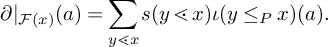 $$ \begin{align*}\partial\vert_{\mathcal{F}(x)}(a)=\sum_{y\lessdot x}s(y\lessdot x)\iota(y\leq_P x)(a). \end{align*} $$
Since the poset is thin, we have $\partial ^2=0$
. The homology groups of
$\partial ^2=0$
. The homology groups of $(C_\bullet (P;\mathcal {F}),\partial )$
are denoted as usual by
$(C_\bullet (P;\mathcal {F}),\partial )$
are denoted as usual by $H_\bullet (P;\mathcal {F})$
. If a subset U of P is closed under taking larger elements (sometimes U is called open), one can restrict the differential complex and the homology groups to U. We denote this restriction by
$H_\bullet (P;\mathcal {F})$
. If a subset U of P is closed under taking larger elements (sometimes U is called open), one can restrict the differential complex and the homology groups to U. We denote this restriction by $C_\bullet (U;\mathcal {F})$
and
$C_\bullet (U;\mathcal {F})$
and $H_\bullet (U;\mathcal {F})$
. Also maps of cosheaves induce maps between homology groups, and short exact sequences of cosheaves induce long exact sequences of homology groups.
$H_\bullet (U;\mathcal {F})$
. Also maps of cosheaves induce maps between homology groups, and short exact sequences of cosheaves induce long exact sequences of homology groups.
2.5 Tropical homology
Tropical homology is a homology theory with non-constant coefficients defined over tropical varieties [Reference Itenberg, Katzarkov, Mikhalkin and Zharkov16], [Reference Brugallé, López de Medrano and Rau8]. In our case, if T and $T^\circ $
are convex primitive central triangulations of
$T^\circ $
are convex primitive central triangulations of $\Delta $
and
$\Delta $
and $\Delta ^\circ $
, respectively, the tropical varieties
$\Delta ^\circ $
, respectively, the tropical varieties $X_{\text {trop}}\subset \mathbb {T}\Sigma _{T^\circ }$
and
$X_{\text {trop}}\subset \mathbb {T}\Sigma _{T^\circ }$
and $X_{\text {trop}}^\circ \subset \mathbb {T}\Sigma _{T}$
of Definition 2.4 are non-singular projective tropical varieties. The tropical homology groups are denoted by
$X_{\text {trop}}^\circ \subset \mathbb {T}\Sigma _{T}$
of Definition 2.4 are non-singular projective tropical varieties. The tropical homology groups are denoted by $H_q(X_{\text {trop}}; \mathcal {F}_p)$
, and it follows from [Reference Itenberg, Katzarkov, Mikhalkin and Zharkov16] that
$H_q(X_{\text {trop}}; \mathcal {F}_p)$
, and it follows from [Reference Itenberg, Katzarkov, Mikhalkin and Zharkov16] that
 $$ \begin{align*}\dim H_q(X_{\text{trop}};\mathcal{F}_p\otimes\mathbb{Q})=h^{p,q}(X) \text{ and } \dim H_q(X_{\text{trop}}^\circ;\mathcal{F}_p\otimes \mathbb{Q})=h^{p,q}(X^\circ). \end{align*} $$
Here, X and $X^\circ $
are any smooth anticanonical hypersurfaces in
$X^\circ $
are any smooth anticanonical hypersurfaces in $\mathbb {C} \Sigma _{T^\circ }$
and
$\mathbb {C} \Sigma _{T^\circ }$
and $\mathbb {C} \Sigma _{T}$
, respectively. Tropical homology (in its cellular version) belongs to the realm of poset homology.
$\mathbb {C} \Sigma _{T}$
, respectively. Tropical homology (in its cellular version) belongs to the realm of poset homology.
We fix T and $T^\circ $
not necessarily convex primitive central triangulations of
$T^\circ $
not necessarily convex primitive central triangulations of $\Delta $
and
$\Delta $
and $\Delta ^\circ $
, respectively. The poset
$\Delta ^\circ $
, respectively. The poset $\mathcal {P}(T^\circ ,T)$
is graded by the formula
$\mathcal {P}(T^\circ ,T)$
is graded by the formula
 $$ \begin{align*}\dim(\tau,\sigma)=\operatorname{\mathrm{codim}}(\tau)-\dim(\sigma). \end{align*} $$
Note that $\dim (\tau ,\sigma )=\dim F(\tau ,\sigma )$
in the geometric realization of
$\dim (\tau ,\sigma )=\dim F(\tau ,\sigma )$
in the geometric realization of $\mathcal {P}(T^\circ ,T)$
. Moreover, the poset
$\mathcal {P}(T^\circ ,T)$
. Moreover, the poset $\mathcal {P}(T^\circ ,T)$
is thin, and it admits a balanced signature, obtained by choosing orientations on each
$\mathcal {P}(T^\circ ,T)$
is thin, and it admits a balanced signature, obtained by choosing orientations on each $F(\tau ,\sigma )$
. The p-multitangent cosheaves over
$F(\tau ,\sigma )$
. The p-multitangent cosheaves over $\mathcal P(T^\circ ,T)$
are defined by
$\mathcal P(T^\circ ,T)$
are defined by
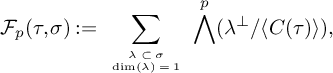 $$ \begin{align*}\mathcal{F}_p(\tau,\sigma):=\sum_{ \tiny{\begin{array}{c} \lambda\subset\sigma \\ \dim(\lambda)=1 \end{array}}} \bigwedge^p (\lambda^\perp / \langle C(\tau) \rangle ) , \end{align*} $$
where $\langle C(\tau ) \rangle $
is the submodule generated by
$\langle C(\tau ) \rangle $
is the submodule generated by $C(\tau ) \cap N$
. The cosheaf maps of
$C(\tau ) \cap N$
. The cosheaf maps of $\mathcal {F}_p$
are induced by the projections
$\mathcal {F}_p$
are induced by the projections
 $$ \begin{align} N /\langle C(\tau) \rangle \rightarrow N /\langle C(\tau') \rangle \end{align} $$
if $\tau \subset \tau '$
(recall that by definition of
$\tau \subset \tau '$
(recall that by definition of $\mathcal P(T^\circ ,T)$
, the faces
$\mathcal P(T^\circ ,T)$
, the faces $\tau $
and
$\tau $
and $\tau '$
contain
$\tau '$
contain $0$
). Note that the support of the cosheaves
$0$
). Note that the support of the cosheaves $\mathcal {F}_p$
is the poset
$\mathcal {F}_p$
is the poset $\mathcal P^1(T^\circ ,T)$
. In order to lighten the notations, if
$\mathcal P^1(T^\circ ,T)$
. In order to lighten the notations, if $\mathcal {G}$
is any cosheaf on
$\mathcal {G}$
is any cosheaf on $\mathcal P^1(T^\circ ,T)$
, we will denote by
$\mathcal P^1(T^\circ ,T)$
, we will denote by $H_\bullet (X_{T^\circ ,T};\mathcal {G})$
the homology groups
$H_\bullet (X_{T^\circ ,T};\mathcal {G})$
the homology groups $H_\bullet (\mathcal P^1(T^\circ ,T);\mathcal {G})$
.
$H_\bullet (\mathcal P^1(T^\circ ,T);\mathcal {G})$
.
3 Combinatorial mirror symmetry
Define $\mathcal {P}^\infty (T^\circ ,T)$
to be the subposet of
$\mathcal {P}^\infty (T^\circ ,T)$
to be the subposet of $\mathcal {P}(T^\circ ,T)$
consisting of elements whose first coordinate is nonzero. Its elements parametrize the boundary of
$\mathcal {P}(T^\circ ,T)$
consisting of elements whose first coordinate is nonzero. Its elements parametrize the boundary of $\mathbb {T}\Sigma _{T^\circ }$
.
$\mathbb {T}\Sigma _{T^\circ }$
.
Lemma 3.1. The map
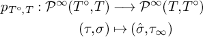 $$ \begin{align} \begin{aligned} p_{T^\circ,T}: \mathcal{P}^\infty(T^\circ, T) & \longrightarrow \mathcal{P}^\infty(T , T^\circ) \\ (\tau,\sigma) & \mapsto (\hat{\sigma},\tau_\infty) \end{aligned} \end{align} $$
is an isomorphism of posets.
Proof. The map $p_{T^\circ ,T}$
is clearly invertible with inverse
$p_{T^\circ ,T}$
is clearly invertible with inverse $p_{T,T^\circ }$
. We only have to verify that if
$p_{T,T^\circ }$
. We only have to verify that if $\sigma \subset \min (C(\tau ))^\vee $
, then
$\sigma \subset \min (C(\tau ))^\vee $
, then $\tau _\infty \subset \min (C(\hat {\sigma }))^\vee $
. Let us say that
$\tau _\infty \subset \min (C(\hat {\sigma }))^\vee $
. Let us say that $\min (C(\tau ))=\operatorname {\mathrm {Cone}}(u_1,\cdots ,u_r)$
and that
$\min (C(\tau ))=\operatorname {\mathrm {Cone}}(u_1,\cdots ,u_r)$
and that $\min (C(\hat {\sigma }))=\operatorname {\mathrm {Cone}}(v_1,\cdots ,v_s)$
, where the
$\min (C(\hat {\sigma }))=\operatorname {\mathrm {Cone}}(v_1,\cdots ,v_s)$
, where the $u_i$
’s in N and the
$u_i$
’s in N and the $v_j$
’s in M are respectively primitive generators of the rays of
$v_j$
’s in M are respectively primitive generators of the rays of $\min (C(\tau ))$
and
$\min (C(\tau ))$
and $\min (C(\hat {\sigma }))$
. Then since
$\min (C(\hat {\sigma }))$
. Then since $\sigma \subset \min (C(\tau ))^\vee $
and by reflexivity, one has that
$\sigma \subset \min (C(\tau ))^\vee $
and by reflexivity, one has that
 $$ \begin{align*}\langle u_i,x \rangle =1, \quad \forall x\in\sigma \text{ and } \forall i. \end{align*} $$
Moreover, the same equality is true for any x in the minimal face of $\Delta ^{\circ }$
containing
$\Delta ^{\circ }$
containing $\sigma $
. So one has that
$\sigma $
. So one has that $\langle u_i,v_j \rangle =1$
for all
$\langle u_i,v_j \rangle =1$
for all $i,j$
. Now if
$i,j$
. Now if $x\in \tau _\infty $
, then
$x\in \tau _\infty $
, then $x=\sum \alpha _i u_i$
with
$x=\sum \alpha _i u_i$
with $\sum \alpha _i=1$
. Then for all j, we obtain that
$\sum \alpha _i=1$
. Then for all j, we obtain that $\langle x,v_j \rangle =\sum \alpha _i \langle u_i,v_j \rangle =1$
.
$\langle x,v_j \rangle =\sum \alpha _i \langle u_i,v_j \rangle =1$
.
Example 3.2. In Figure 2, we represented the geometric realization of the poset $\mathcal {P}(T,T^\circ )$
, where T and
$\mathcal {P}(T,T^\circ )$
, where T and $T^\circ $
are defined as in Example 2.5, with some examples of cells. Notice that the cells
$T^\circ $
are defined as in Example 2.5, with some examples of cells. Notice that the cells $(\tau _2, \sigma _2)$
and
$(\tau _2, \sigma _2)$
and $(\tau _3, \sigma _3)$
appearing in Figure 2 correspond, under the map
$(\tau _3, \sigma _3)$
appearing in Figure 2 correspond, under the map $p_{T^\circ ,T}$
, to the cells with the same label in Figure 1.
$p_{T^\circ ,T}$
, to the cells with the same label in Figure 1.
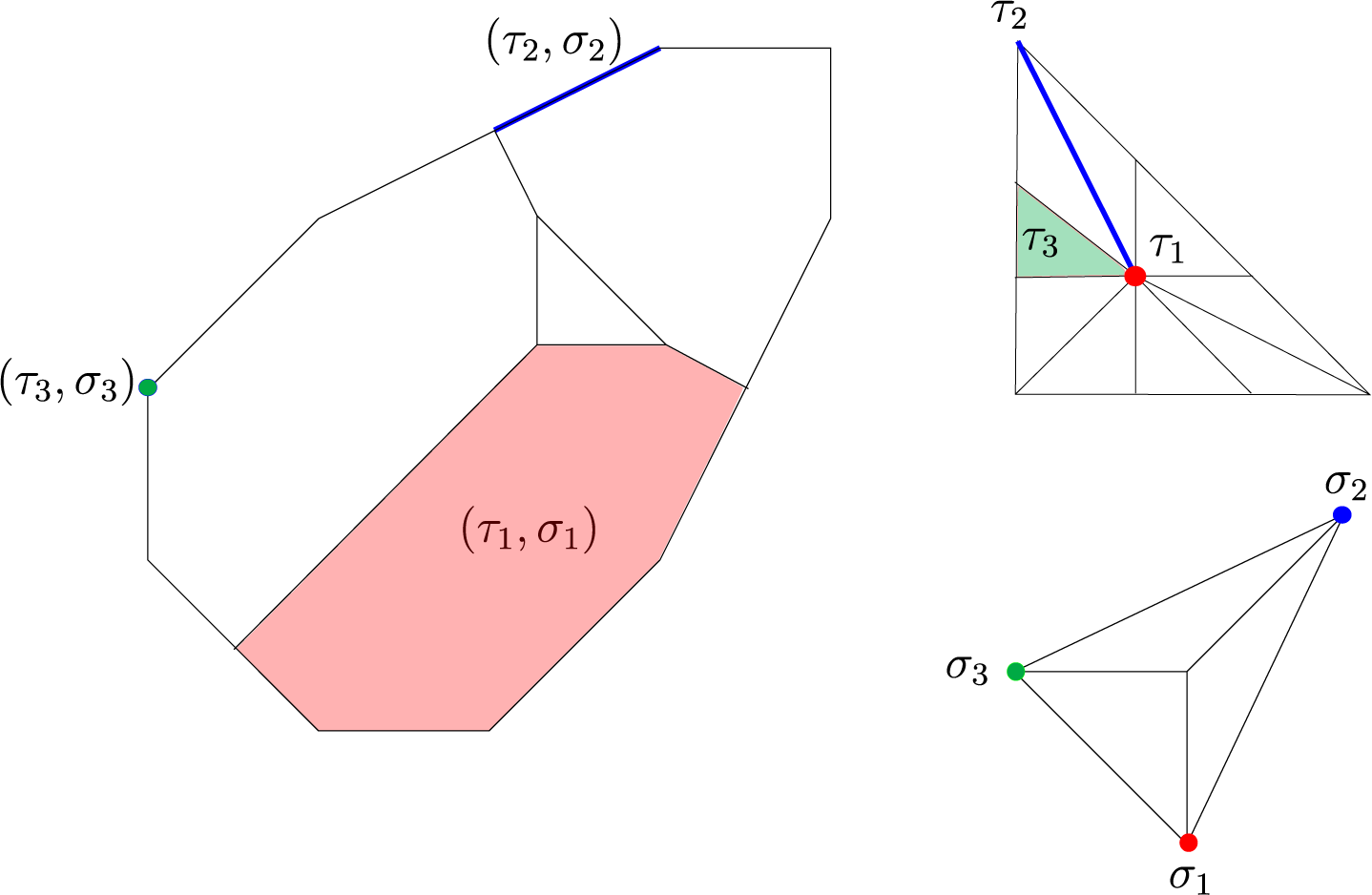
Figure 2 The subdivision $\mathcal {P}(T,T^\circ )$
.
$\mathcal {P}(T,T^\circ )$
.
We will next refine the poset $\mathcal {P}(T^\circ ,T)$
, in order to extend this correspondence to the whole poset minus the origin.
$\mathcal {P}(T^\circ ,T)$
, in order to extend this correspondence to the whole poset minus the origin.
3.1 A refinement of the poset
$\mathcal {P}(T^\circ ,T)$

Definition 3.3. The poset $\mathcal {J}(T^\circ ,T)$
is the subposet of
$\mathcal {J}(T^\circ ,T)$
is the subposet of $T^\circ \times T$
defined by the following:
$T^\circ \times T$
defined by the following:
-
• If
$\sigma \neq 0$
and
$0\in \sigma $
, then consider all pairs
$(\tau ,\sigma )$
such that
$\tau \in \partial T^\circ $
and
$\sigma _\infty \subset \min (C(\tau ))^\vee $
. -
• If
$\sigma \in \partial T$
, consider all pairs
$(\tau ,\sigma )$
such that
$\tau \neq 0$
and
$\sigma \subset \min (C(\tau ))^\vee $
.


Define $\mathcal {J}^S(T^\circ ,T)$
the subposet of
$\mathcal {J}^S(T^\circ ,T)$
the subposet of $\mathcal {J}(T^\circ ,T)$
consisting of pairs of the first kind, and by
$\mathcal {J}(T^\circ ,T)$
consisting of pairs of the first kind, and by $\mathcal {J}^\infty (T^\circ ,T)$
the subposet of
$\mathcal {J}^\infty (T^\circ ,T)$
the subposet of $\mathcal {J}(T^\circ ,T)$
consisting of pairs
$\mathcal {J}(T^\circ ,T)$
consisting of pairs $(\tau ,\sigma )$
such that
$(\tau ,\sigma )$
such that $0\in \tau $
.
$0\in \tau $
.
Notice that we do not consider the pair $(0,0)$
in
$(0,0)$
in $\mathcal {J}(T^\circ ,T)$
. In fact, by definition, the pair
$\mathcal {J}(T^\circ ,T)$
. In fact, by definition, the pair $(0,0)$
would be isolated (i.e., not comparable to any other pair inside
$(0,0)$
would be isolated (i.e., not comparable to any other pair inside $\mathcal {J}(T^\circ ,T)$
).
$\mathcal {J}(T^\circ ,T)$
).
It follows from the definition that the map from $\mathcal {J}(T^\circ ,T)$
to
$\mathcal {J}(T^\circ ,T)$
to $\mathcal {P}(T^\circ ,T)\setminus (0,0)$
sending
$\mathcal {P}(T^\circ ,T)\setminus (0,0)$
sending $(\tau ,\sigma )$
to
$(\tau ,\sigma )$
to $(0,\sigma )$
if
$(0,\sigma )$
if $0\notin \tau $
, and to itself if
$0\notin \tau $
, and to itself if $0\in \tau $
is surjective. The poset
$0\in \tau $
is surjective. The poset $\mathcal {J}(T^\circ ,T)$
is still a graded poset (with the same grading as before), is thin and still admits a balanced signature. In fact, its geometric realization (as defined above) is a subdivision of the one of
$\mathcal {J}(T^\circ ,T)$
is still a graded poset (with the same grading as before), is thin and still admits a balanced signature. In fact, its geometric realization (as defined above) is a subdivision of the one of $\mathcal {P}(T^\circ ,T)$
(minus the cell
$\mathcal {P}(T^\circ ,T)$
(minus the cell $F(0,0)$
). Similarly, the geometric realization of
$F(0,0)$
). Similarly, the geometric realization of $\mathcal {J}^S(T^\circ ,T)$
is a subdivision of
$\mathcal {J}^S(T^\circ ,T)$
is a subdivision of $S_{T^\circ ,T}$
, and
$S_{T^\circ ,T}$
, and $\mathcal {J}^\infty (T^\circ ,T)=\mathcal {P}^\infty (T^\circ ,T)$
. As a corollary of Lemma 3.1, one obtains the following:
$\mathcal {J}^\infty (T^\circ ,T)=\mathcal {P}^\infty (T^\circ ,T)$
. As a corollary of Lemma 3.1, one obtains the following:
Lemma 3.4. The map
 $$ \begin{align} j_{T^\circ,T}: \mathcal{J}(T^\circ, T) \longrightarrow \mathcal{J}(T , T^\circ) \end{align} $$
sending
-
•
$(\tau ,\sigma )$
to
$(\hat {\sigma },\tau _\infty )$
if
$0\in \tau $
and
$\sigma \in \partial T$
, -
•
$(\tau ,\sigma )$
to
$(\sigma _\infty ,\hat {\tau })$
if
$\tau \in \partial T^\circ $
and
$0\in \sigma $
, and -
•
$(\tau ,\sigma )$
to
$(\sigma ,\tau )$
if
$(\tau ,\sigma )\in \partial T^\circ \times \partial T$


is an isomorphism of posets.
Notice that $j_{T^\circ ,T}$
sends
$j_{T^\circ ,T}$
sends $\mathcal {J}^S(T^\circ ,T)$
to
$\mathcal {J}^S(T^\circ ,T)$
to $\mathcal {J}^S(T,T^\circ )$
, sends
$\mathcal {J}^S(T,T^\circ )$
, sends $\mathcal {J}^\infty (T^\circ ,T)$
to
$\mathcal {J}^\infty (T^\circ ,T)$
to $\mathcal {J}^\infty (T,T^\circ )$
and preserves the dimensions.
$\mathcal {J}^\infty (T,T^\circ )$
and preserves the dimensions.
Example 3.5. In Figures 3 and 4, we represented the geometric realizations of the posets $\mathcal {J}(T,T^\circ )$
and
$\mathcal {J}(T,T^\circ )$
and $\mathcal {J}(T^\circ , T)$
, where T and
$\mathcal {J}(T^\circ , T)$
, where T and $T^\circ $
are defined again as in Example 2.5. The cells depicted in the two figures are dual in the sense that they correspond under the map
$T^\circ $
are defined again as in Example 2.5. The cells depicted in the two figures are dual in the sense that they correspond under the map $j_{T^\circ ,T}$
.
$j_{T^\circ ,T}$
.
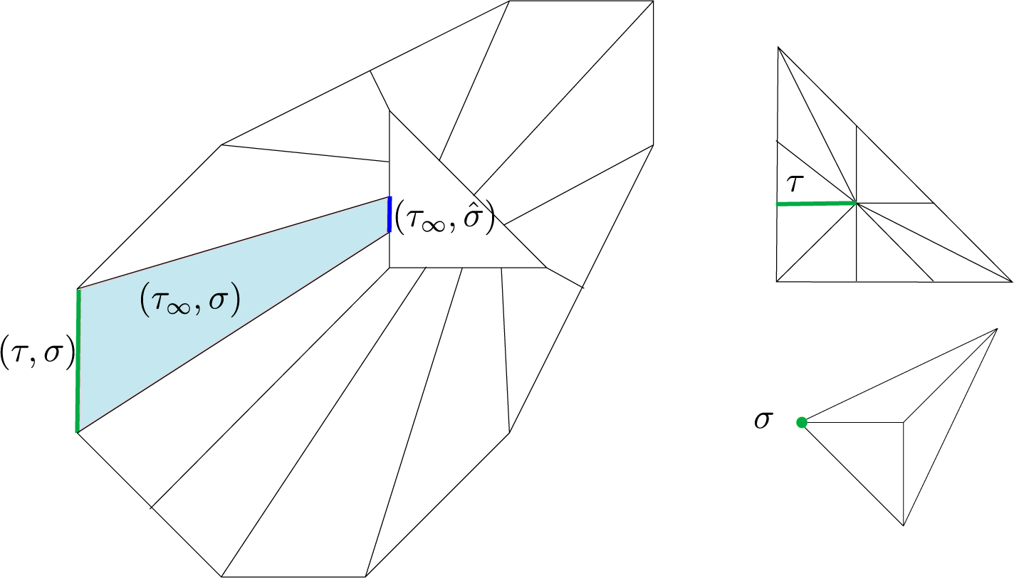
Figure 3 The subdivision $\mathcal {J}(T,T^\circ )$
.
$\mathcal {J}(T,T^\circ )$
.
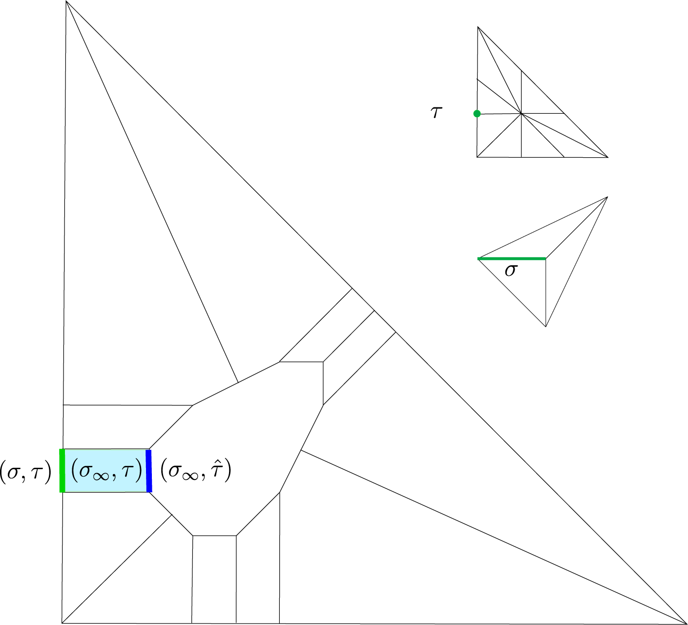
Figure 4 The subdivision $\mathcal {J}(T^\circ , T)$
.
$\mathcal {J}(T^\circ , T)$
.
We extend the cosheaves $\mathcal {F}_p(\tau ,\sigma )$
to the poset
$\mathcal {F}_p(\tau ,\sigma )$
to the poset $\mathcal {J}(T^{\circ }, T)$
by precomposing with the map from above sending
$\mathcal {J}(T^{\circ }, T)$
by precomposing with the map from above sending $(\tau ,\sigma )$
to
$(\tau ,\sigma )$
to $(0,\sigma )$
if
$(0,\sigma )$
if $0\notin \tau $
and to itself if
$0\notin \tau $
and to itself if $0\in \tau $
. Define as before
$0\in \tau $
. Define as before
 $$ \begin{align*}\mathcal{J}^1(T^\circ, T):=\left\lbrace (\tau,\sigma)\in \mathcal{J}(T^\circ, T) \vert \dim(\sigma)\geq 1 \right\rbrace. \end{align*} $$
The geometric realization of $\mathcal {J}^1(T^\circ , T)$
defines a subdivision of
$\mathcal {J}^1(T^\circ , T)$
defines a subdivision of $X_{T^\circ ,T}$
, and it is the support of the cosheaf
$X_{T^\circ ,T}$
, and it is the support of the cosheaf $\mathcal {F}_p$
. One has a canonical isomorphism
$\mathcal {F}_p$
. One has a canonical isomorphism
 $$ \begin{align*}H_q(\mathcal{J}(T^\circ,T); \mathcal F_p) \cong H_q(X_{T^\circ,T}; \mathcal F_p). \end{align*} $$
3.2 The mirror cosheaf
Let $(\tau ,\sigma )\in \mathcal {J}^S(T^\circ ,T)$
. Since
$(\tau ,\sigma )\in \mathcal {J}^S(T^\circ ,T)$
. Since $\sigma _\infty \subset \min (C(\tau ))^\vee $
, in particular, the cone
$\sigma _\infty \subset \min (C(\tau ))^\vee $
, in particular, the cone $C(\tau )$
is a subset of
$C(\tau )$
is a subset of $\sigma _\infty ^\perp $
. Then
$\sigma _\infty ^\perp $
. Then $\langle C(\tau ) \rangle \wedge \mathcal {F}_{p-1}(0,\sigma _{\infty })$
is a submodule of
$\langle C(\tau ) \rangle \wedge \mathcal {F}_{p-1}(0,\sigma _{\infty })$
is a submodule of $\mathcal {F}_p(0,\sigma )$
, and we can consider the quotient.
$\mathcal {F}_p(0,\sigma )$
, and we can consider the quotient.
Definition 3.6. Let $p\geq 0$
. The p-th mirror cosheaf
$p\geq 0$
. The p-th mirror cosheaf $\mathcal {M}_p$
is defined over
$\mathcal {M}_p$
is defined over $\mathcal {J}(T^\circ ,T)$
as follows:
$\mathcal {J}(T^\circ ,T)$
as follows:
-
• if
$\sigma \neq 0$
and
$0\in \sigma $
, then define (11)where
$$ \begin{align} \mathcal{M}_p(\tau, \sigma)=\frac{\mathcal{F}_p(0,\sigma)} { \langle C(\tau) \rangle \wedge \mathcal{F}_{p-1}(0,\sigma_{\infty})}, \end{align} $$
$\langle C(\tau ) \rangle $
is the submodule generated by
$C(\tau ) \cap N$
. When
$p=0$
, we define
$\mathcal {M}_0(\tau , \sigma ) = \mathbb {Z}$
.
-
• for all other elements
$(\tau ,\sigma ) \in \mathcal {J}(T^\circ ,T)$
, set (12)
$$ \begin{align} \mathcal{M}_p( \tau, \sigma)=0. \end{align} $$


The cosheaf maps are induced by the ones from $\mathcal {F}_p$
.
$\mathcal {F}_p$
.
Notice that the support of $\mathcal {M}_p$
is
$\mathcal {M}_p$
is $\mathcal {J}^S (T^\circ ,T)$
and that, moreover,
$\mathcal {J}^S (T^\circ ,T)$
and that, moreover,
 $$\begin{align*}\mathcal M_p(\tau, \sigma) = \mathcal F_p(0, \sigma) \quad \text{when } 0\in\sigma \text{ and } \dim \sigma = 1.\end{align*}$$
We have the following main result:
Theorem 3.7. Let A be a commutative ring. For all $q \geq 0$
, there are canonical isomorphisms
$q \geq 0$
, there are canonical isomorphisms
 $$ \begin{align} H_q(\mathcal{J}(T^\circ,T); \mathcal F_p\otimes A) \cong H_q(\mathcal{J}(T^\circ,T); \mathcal M_p\otimes A), \end{align} $$
 $$ \begin{align} H_q(\mathcal{J}(T^\circ,T); \mathcal M_p\otimes A) \cong H_q(\mathcal{J}(T,T^\circ); \mathcal M_{n-p}\otimes A). \end{align} $$
Moreover, they induce a canonical isomorphism
 $$ \begin{align} H_q(X_{T^\circ,T}; \mathcal F_p\otimes A) \cong H_q(X_{T,T^\circ}; \mathcal F_{n-p}\otimes A). \end{align} $$
Corollary 3.8. If T and $T^\circ $
are convex subdivisions, and
$T^\circ $
are convex subdivisions, and $X_{\text {trop}}$
and
$X_{\text {trop}}$
and $X^\circ _{\text {trop}}$
are some correponding tropical hypersurfaces as in Definition 2.4, then we have the mirror symmetry of the tropical Hodge diamonds
$X^\circ _{\text {trop}}$
are some correponding tropical hypersurfaces as in Definition 2.4, then we have the mirror symmetry of the tropical Hodge diamonds
 $$\begin{align*}\dim H_q( X_{\text{trop}}; \mathcal F_p\otimes \mathbb{Q}) = \dim H_q(X^{\circ}_{\text{trop}}; \mathcal F_{n-p}\otimes \mathbb{Q}). \end{align*}$$
Definition 3.9 (Mirror classes).
Two classes $\gamma \in H_q(\mathcal {P}(T^\circ ,T); \mathcal F_p\otimes A)$
and
$\gamma \in H_q(\mathcal {P}(T^\circ ,T); \mathcal F_p\otimes A)$
and $\gamma '\in H_q (\mathcal {P}(T, T^\circ ); \mathcal F_{n-p}\otimes A)$
are called mirror classes if they coincide under isomorphism (15).
$\gamma '\in H_q (\mathcal {P}(T, T^\circ ); \mathcal F_{n-p}\otimes A)$
are called mirror classes if they coincide under isomorphism (15).
3.3 Proof of Theorem 3.7
We begin by extending the support of $\mathcal {M}_p$
to the whole poset
$\mathcal {M}_p$
to the whole poset $\mathcal {J}(T^\circ ,T)$
.
$\mathcal {J}(T^\circ ,T)$
.
Definition 3.10. Let $p\geq 0$
. The cosheaf
$p\geq 0$
. The cosheaf $\mathcal {M}_p^{\Delta }$
is defined over
$\mathcal {M}_p^{\Delta }$
is defined over $\mathcal {J}(T^\circ ,T)$
by
$\mathcal {J}(T^\circ ,T)$
by
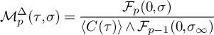 $$ \begin{align} \mathcal{M}_p^{\Delta}(\tau, \sigma)=\dfrac{\mathcal{F}_p(0,\sigma )}{\langle C(\tau) \rangle \wedge \mathcal{F}_{p-1}(0,\sigma_\infty)} \end{align} $$
if $\tau \in \partial T^\circ $
, and by
$\tau \in \partial T^\circ $
, and by $\mathcal F_p$
otherwise. Notice that
$\mathcal F_p$
otherwise. Notice that
 $$\begin{align*}\mathcal{M}_p^{\Delta}(\tau, \sigma ) = \mathcal{M}_p(\tau, \sigma ) \quad \text{when} \ (\tau, \sigma) \in \mathcal{J}^{S}(T^\circ,T) \end{align*}$$
and
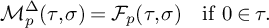 $$\begin{align*}\mathcal{M}_p^{\Delta}(\tau, \sigma ) = \mathcal{F}_p(\tau ,\sigma ) \quad \text{if} \ 0\in \tau. \end{align*}$$
By definition, we have an inclusion $\mathcal {M}_p \hookrightarrow \mathcal {M}_p^{\Delta }$
and a surjection
$\mathcal {M}_p \hookrightarrow \mathcal {M}_p^{\Delta }$
and a surjection $\mathcal F_p \rightarrow \mathcal M_p^{\Delta }$
. These give two short exact sequences of cosheaves
$\mathcal F_p \rightarrow \mathcal M_p^{\Delta }$
. These give two short exact sequences of cosheaves
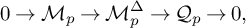 $$ \begin{align} 0 \rightarrow \mathcal M_p \rightarrow \mathcal M_p^{\Delta} \rightarrow \mathcal Q_p \rightarrow 0, \end{align} $$
where $\mathcal Q_p$
is the quotient cosheaf, and
$\mathcal Q_p$
is the quotient cosheaf, and
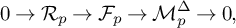 $$ \begin{align} 0 \rightarrow \mathcal R_p \rightarrow \mathcal F_p \rightarrow \mathcal M_p^{\Delta} \rightarrow 0, \end{align} $$
where $\mathcal R_p$
is the kernel.
$\mathcal R_p$
is the kernel.
The quotient $\mathcal {Q}_p$
is given by
$\mathcal {Q}_p$
is given by $\mathcal {Q}_p(\tau , \sigma )=\mathcal {M}_p^{\Delta }(\tau , \sigma )$
if
$\mathcal {Q}_p(\tau , \sigma )=\mathcal {M}_p^{\Delta }(\tau , \sigma )$
if $\sigma \in \partial T$
and is equal to zero otherwise. In particular,
$\sigma \in \partial T$
and is equal to zero otherwise. In particular, $\mathcal Q_p$
is supported on
$\mathcal Q_p$
is supported on
 $$\begin{align*}\mathcal{J}^{ub}(T^\circ,T):=\mathcal{J}(T^\circ,T)\setminus \mathcal{J}^S(T^\circ,T). \end{align*}$$
The kernel $\mathcal {R}_p$
is given by
$\mathcal {R}_p$
is given by $\mathcal {R}_p(\tau ,\sigma )=\langle C(\tau ) \rangle \wedge \mathcal {F}_{p-1}(0,\sigma _\infty )$
if
$\mathcal {R}_p(\tau ,\sigma )=\langle C(\tau ) \rangle \wedge \mathcal {F}_{p-1}(0,\sigma _\infty )$
if $\tau \in \partial T^\circ $
and is equal to zero otherwise. The support of
$\tau \in \partial T^\circ $
and is equal to zero otherwise. The support of $\mathcal {R}_p$
is
$\mathcal {R}_p$
is
 $$\begin{align*}\mathcal{J}^{0}(T^\circ,T):=\mathcal{J}(T^\circ,T)\setminus \mathcal{J}^\infty(T^\circ,T). \end{align*}$$
We have the following:
Proposition 3.11. The cosheaves $\mathcal M_p$
,
$\mathcal M_p$
, $\mathcal M_p^{\Delta }$
,
$\mathcal M_p^{\Delta }$
, $\mathcal {Q}_p$
and
$\mathcal {Q}_p$
and $\mathcal R_p$
are cosheaves of free
$\mathcal R_p$
are cosheaves of free $\mathbb {Z}$
-modules. Moreover, let
$\mathbb {Z}$
-modules. Moreover, let $\sigma \in \partial T$
and
$\sigma \in \partial T$
and $\tau \in \partial T^\circ $
such that
$\tau \in \partial T^\circ $
such that $\sigma \subset \min (C(\tau ))^\vee $
. Then the cosheaf maps
$\sigma \subset \min (C(\tau ))^\vee $
. Then the cosheaf maps
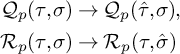 $$\begin{align*}\begin{aligned} \mathcal Q_p(\tau, \sigma) & \rightarrow \mathcal Q_p (\hat{\tau}, \sigma), \\ \mathcal R_p(\tau, \sigma) & \rightarrow \mathcal R_p (\tau, \hat{\sigma} ) \end{aligned} \end{align*}$$
are isomorphisms.
Proof. It is easy to see that $\mathcal F_p$
is a cosheaf of free
$\mathcal F_p$
is a cosheaf of free $\mathbb {Z}$
-modules and therefore also
$\mathbb {Z}$
-modules and therefore also $\mathcal R_p$
. It is then enough to show that
$\mathcal R_p$
. It is then enough to show that $\mathcal M^{\Delta }_p$
is a cosheaf of free modules.
$\mathcal M^{\Delta }_p$
is a cosheaf of free modules.
Let $(\tau , \sigma ) \in \mathcal {J}(T^\circ ,T)$
with
$(\tau , \sigma ) \in \mathcal {J}(T^\circ ,T)$
with $0 \in \sigma $
and
$0 \in \sigma $
and $\tau \in \partial T^{\circ }$
. We begin by describing bases for
$\tau \in \partial T^{\circ }$
. We begin by describing bases for $\mathcal F_p(0, \sigma )$
,
$\mathcal F_p(0, \sigma )$
, $\mathcal F_p(0, \sigma _{\infty })$
and
$\mathcal F_p(0, \sigma _{\infty })$
and $\langle C(\tau ) \rangle \wedge \mathcal {F}_{p-1} (0,\sigma _{\infty })$
. The cell
$\langle C(\tau ) \rangle \wedge \mathcal {F}_{p-1} (0,\sigma _{\infty })$
. The cell $\sigma $
is a primitive simplex; let
$\sigma $
is a primitive simplex; let $\dim \sigma = s+1$
. Choose a vertex
$\dim \sigma = s+1$
. Choose a vertex $e_0$
of
$e_0$
of $\sigma _{\infty }$
and fix s edges of
$\sigma _{\infty }$
and fix s edges of $\sigma _{\infty }$
containing this vertex. Denote by
$\sigma _{\infty }$
containing this vertex. Denote by $e_1,\cdots ,e_{s}$
a choice of primitive vectors directing those edges. Complete the set
$e_1,\cdots ,e_{s}$
a choice of primitive vectors directing those edges. Complete the set $e_1, \ldots , e_{s}$
to a basis of
$e_1, \ldots , e_{s}$
to a basis of $\langle C(\tau )\rangle ^\perp $
denoted by
$\langle C(\tau )\rangle ^\perp $
denoted by $e_1,\cdots ,e_m$
, and complete the set
$e_1,\cdots ,e_m$
, and complete the set $e_0, \ldots , e_m$
to a basis of M denoted by
$e_0, \ldots , e_m$
to a basis of M denoted by $e_0,\cdots ,e_{n}$
. Consider the dual basis
$e_0,\cdots ,e_{n}$
. Consider the dual basis $e_0^*,\cdots ,e_{n}^*$
of N. We have
$e_0^*,\cdots ,e_{n}^*$
of N. We have
 $$ \begin{align*}\langle C(\tau) \rangle = \langle e_0^*, e_{m+1}^*,\cdots,e_{n}^*\rangle.\end{align*} $$
We use multi-indices $I=\{ i_1, \ldots , i_p \} \subseteq \{0, \ldots , n \}$
with
$I=\{ i_1, \ldots , i_p \} \subseteq \{0, \ldots , n \}$
with $i_1 < i_2 < \ldots < i_p$
, and we denote by
$i_1 < i_2 < \ldots < i_p$
, and we denote by $e_I^*$
the p-vector
$e_I^*$
the p-vector $e_{i_1}^* \wedge \ldots \wedge e_{i_p}^*$
. We also denote by
$e_{i_1}^* \wedge \ldots \wedge e_{i_p}^*$
. We also denote by $|I|$
the cardinality of I and by
$|I|$
the cardinality of I and by $I^c$
the complement of I in
$I^c$
the complement of I in $\{0, \ldots , n \}$
. A basis of
$\{0, \ldots , n \}$
. A basis of $\mathcal F_p(0, \sigma )$
consists of p-vectors of the type
$\mathcal F_p(0, \sigma )$
consists of p-vectors of the type
 $$ \begin{align*}e_I^*, \quad \ I^c \cap \{0, \ldots, s \} \neq \emptyset. \end{align*} $$
Similarly, a basis of $\mathcal F_{p-1}(0, \sigma _{\infty })$
is given by the
$\mathcal F_{p-1}(0, \sigma _{\infty })$
is given by the $p-1$
-vectors
$p-1$
-vectors
 $$ \begin{align*}e_J^*, \quad J^c \cap \{1, \ldots, s \} \neq \emptyset. \end{align*} $$
Then a basis of $\langle C(\tau ) \rangle \wedge \mathcal {F}_{p-1}(0,\sigma _{\infty })$
is given by p-vectors of the type
$\langle C(\tau ) \rangle \wedge \mathcal {F}_{p-1}(0,\sigma _{\infty })$
is given by p-vectors of the type
 $$ \begin{align*}e_I^*, \quad I \cap \{0, m+1, \ldots, n \} \neq \emptyset \ \text{and} \ I^c \cap \{1, \ldots, s \} \neq \emptyset. \end{align*} $$
This clearly shows that $\mathcal M_{p}^{\Delta }$
is free.
$\mathcal M_{p}^{\Delta }$
is free.
Assume now that $\tau \in \partial T^\circ $
and
$\tau \in \partial T^\circ $
and $\sigma \in \partial T$
(in particular,
$\sigma \in \partial T$
(in particular, $\sigma = \sigma _{\infty }$
). With the same notation as above, the quotient
$\sigma = \sigma _{\infty }$
). With the same notation as above, the quotient $N/ \langle C(\tau ) \rangle $
can be identified with
$N/ \langle C(\tau ) \rangle $
can be identified with $\langle e_1^*,\cdots ,e_m^*\rangle $
. By definition,
$\langle e_1^*,\cdots ,e_m^*\rangle $
. By definition,
 $$ \begin{align*}\mathcal Q_p (\hat{\tau}, \sigma) = \mathcal F_p(\hat{\tau}, \sigma)=\sum_{i=1}^{s} \bigwedge^p (e_i^\perp / \langle C(\tau) \rangle ),\end{align*} $$
so a basis of $\mathcal Q_p(\hat {\tau }, \sigma )$
can be identified with p-vectors of the type
$\mathcal Q_p(\hat {\tau }, \sigma )$
can be identified with p-vectors of the type
 $$ \begin{align*}e_I^*, \quad I \subseteq \{1, \dots, m \} \ \text{and} \ I^c \cap \{1, \ldots, s \} \neq \emptyset, \end{align*} $$
where now $I^c$
denotes the complement of I in
$I^c$
denotes the complement of I in $\{1, \dots , m \}$
. Now notice that also a basis of
$\{1, \dots , m \}$
. Now notice that also a basis of
 $$\begin{align*}\mathcal Q_p (\tau, \sigma) = \mathcal M_p^{\Delta}(\tau, \sigma) = \dfrac{\mathcal{F}_p(0,\sigma )}{\langle C(\tau) \rangle \wedge \mathcal{F}_{p-1}(0,\sigma)}\end{align*}$$
can be identified by the same set of p-vectors, since multi-indices I such that $I \cap \{ 0, m+1, \ldots , n \} \neq \emptyset $
are killed by the quotient. This implies that
$I \cap \{ 0, m+1, \ldots , n \} \neq \emptyset $
are killed by the quotient. This implies that $\mathcal Q_p(\tau , \sigma ) \rightarrow \mathcal Q_p (\hat {\tau }, \sigma )$
is an isomorphism. The case of
$\mathcal Q_p(\tau , \sigma ) \rightarrow \mathcal Q_p (\hat {\tau }, \sigma )$
is an isomorphism. The case of $\mathcal R_p$
is trivial, indeed by definition
$\mathcal R_p$
is trivial, indeed by definition $\mathcal {R}_p(\tau ,\sigma ) = \mathcal {R}_p(\tau , \hat {\sigma })$
.
$\mathcal {R}_p(\tau ,\sigma ) = \mathcal {R}_p(\tau , \hat {\sigma })$
.
We also have the following:
Corollary 3.12. For any commutative ring A, we have short exact sequences
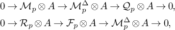 $$\begin{align*}\begin{aligned} \ & 0 \rightarrow \mathcal M_p \otimes A \rightarrow \mathcal M_p^{\Delta} \otimes A \rightarrow \mathcal Q_p \otimes A \rightarrow 0, \\ \ & 0 \rightarrow \mathcal R_p \otimes A \rightarrow \mathcal F_p \otimes A \rightarrow \mathcal M_p^{\Delta} \otimes A \rightarrow 0, \end{aligned} \end{align*}$$
and isomorphisms
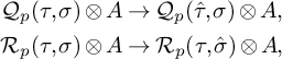 $$\begin{align*}\begin{aligned} \mathcal Q_p(\tau, \sigma) \otimes A & \rightarrow \mathcal Q_p (\hat{\tau}, \sigma) \otimes A, \\ \mathcal R_p(\tau, \sigma) \otimes A & \rightarrow \mathcal R_p (\tau, \hat{\sigma} )\otimes A, \end{aligned} \end{align*}$$
holding for all $\sigma \in \partial T$
and
$\sigma \in \partial T$
and $\tau \in \partial T^\circ $
such that
$\tau \in \partial T^\circ $
such that $\sigma \subset \min (C(\tau ))^\vee $
.
$\sigma \subset \min (C(\tau ))^\vee $
.
Proof. It follows from the fact that if we have a short exact sequence of $\mathbb {Z}$
-modules where the last term is a flat module, then tensoring with any commutative ring preserves exactness. In our case, the modules are free and therefore flat.
$\mathbb {Z}$
-modules where the last term is a flat module, then tensoring with any commutative ring preserves exactness. In our case, the modules are free and therefore flat.
Proposition 3.13. For all $k \geq 0$
and any commutative ring A, we have
$k \geq 0$
and any commutative ring A, we have
 $$\begin{align*}H_k (\mathcal{J}(T^\circ,T); \mathcal Q_p \otimes A) \cong 0, \end{align*}$$
and
 $$\begin{align*}H_k (\mathcal{J}(T^\circ,T); \mathcal R_p \otimes A) \cong 0. \end{align*}$$
Proof. For simplicity, we denote $\mathcal Q_p \otimes A$
and
$\mathcal Q_p \otimes A$
and $\mathcal R_p \otimes A$
by
$\mathcal R_p \otimes A$
by $\mathcal Q_p$
and
$\mathcal Q_p$
and $\mathcal R_p$
. Recall that the support of
$\mathcal R_p$
. Recall that the support of $\mathcal {Q}_p$
is
$\mathcal {Q}_p$
is $\mathcal {J}^{ub}(T^\circ ,T)$
. Introduce
$\mathcal {J}^{ub}(T^\circ ,T)$
. Introduce
 $$ \begin{align*}\mathcal{J}_0^{ub}=\{ (\tau, \sigma) \, | \, \sigma\in \partial T \ \text{and} \ \tau\in \partial T^\circ \} \end{align*} $$
and recall that
 $$ \begin{align*}\mathcal{J}^\infty(T^\circ,T)=\{ (\tau, \sigma) \, | \, \sigma\in \partial T \ \text{and} \ 0\in \tau \}. \end{align*} $$
One has $\mathcal {J}^{ub}(T^\circ ,T)=\mathcal {J}_0^{ub}\cup \mathcal {J}^\infty $
, and there is a bijection between
$\mathcal {J}^{ub}(T^\circ ,T)=\mathcal {J}_0^{ub}\cup \mathcal {J}^\infty $
, and there is a bijection between $\mathcal {J}_0^{ub}$
and
$\mathcal {J}_0^{ub}$
and $\mathcal {J}_\infty $
given by
$\mathcal {J}_\infty $
given by $(\tau ,\sigma ) \mapsto (\hat {\tau },\sigma )$
. Denote by
$(\tau ,\sigma ) \mapsto (\hat {\tau },\sigma )$
. Denote by $\mathcal {C}^{ub}$
the complex of chains
$\mathcal {C}^{ub}$
the complex of chains $\mathcal {C}(\mathcal {J}^{ub}(T^\circ ,T),\mathcal {Q}_p)$
, and similarly by
$\mathcal {C}(\mathcal {J}^{ub}(T^\circ ,T),\mathcal {Q}_p)$
, and similarly by $\mathcal {C}_0^{ub}$
the set of chains supported on
$\mathcal {C}_0^{ub}$
the set of chains supported on $\mathcal {J}_0^{ub}$
and by
$\mathcal {J}_0^{ub}$
and by $\mathcal {C}_\infty $
the complex
$\mathcal {C}_\infty $
the complex $\mathcal {C}(\mathcal {J}^\infty (T^\circ ,T),\mathcal {Q}_p)$
. Notice that
$\mathcal {C}(\mathcal {J}^\infty (T^\circ ,T),\mathcal {Q}_p)$
. Notice that $\mathcal {C}_0^{ub}$
is not closed by taking the boundary. As a module, we have a decomposition
$\mathcal {C}_0^{ub}$
is not closed by taking the boundary. As a module, we have a decomposition
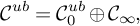 $$\begin{align*}\mathcal C^{ub} = \mathcal C_{0}^{ub} \oplus \mathcal C_{\infty}, \end{align*}$$
and we denote by $\Pi _{0}$
and
$\Pi _{0}$
and $\Pi _{\infty }$
the projections onto the respective component. Proposition 3.11 implies that
$\Pi _{\infty }$
the projections onto the respective component. Proposition 3.11 implies that
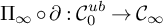 $$ \begin{align} \Pi_{\infty} \circ \partial: \mathcal C_0^{ub} \rightarrow \mathcal C_{\infty} \end{align} $$
is an isomorphism. Denote by $L: \mathcal C_{\infty } \rightarrow \mathcal C_0^{ub}$
its inverse. Suppose now that
$L: \mathcal C_{\infty } \rightarrow \mathcal C_0^{ub}$
its inverse. Suppose now that $\gamma \in \mathcal C^{ub}$
is closed and decompose it as
$\gamma \in \mathcal C^{ub}$
is closed and decompose it as
 $$\begin{align*}\gamma = \gamma_0 + \gamma_{\infty}, \end{align*}$$
its $\mathcal C_0^{ub}$
and
$\mathcal C_0^{ub}$
and $\mathcal C_{\infty }$
components. Then
$\mathcal C_{\infty }$
components. Then
 $$\begin{align*}\partial \gamma_0 = - \partial \gamma_{\infty}. \end{align*}$$
Let
 $$\begin{align*}\beta = L(\gamma_{\infty}). \end{align*}$$
We claim that
 $$\begin{align*}\partial \beta = \gamma. \end{align*}$$
First of all, decomposing $\partial \beta $
and using the fact that L is the inverse of
$\partial \beta $
and using the fact that L is the inverse of $\Pi _{\infty } \circ \partial $
, we have
$\Pi _{\infty } \circ \partial $
, we have
 $$\begin{align*}\partial \beta = \Pi_{0}(\partial \beta) + \gamma_{\infty}. \end{align*}$$
Taking the boundary again, we obtain
 $$\begin{align*}\partial ( \Pi_{0} (\partial \beta)) = - \partial \gamma_{ \infty} = \partial \gamma_0; \end{align*}$$
that is,
 $$\begin{align*}\partial ( \Pi_{0} (\partial \beta) - \gamma_0) = 0. \end{align*}$$
Now the fact that (19) is an isomorphism implies that
 $$\begin{align*}\Pi_{0} (\partial \beta) = \gamma_0. \end{align*}$$
Hence,
 $$\begin{align*}\partial \beta = \gamma, \end{align*}$$
and so any closed chain in $\mathcal {C}^{ub}$
is exact. The proof for
$\mathcal {C}^{ub}$
is exact. The proof for $\mathcal {R}_p$
goes along the exact same lines, by considering the decomposition of
$\mathcal {R}_p$
goes along the exact same lines, by considering the decomposition of $\mathcal {J}^0$
into
$\mathcal {J}^0$
into $\mathcal {J}^{ub}_0 \cup \mathcal {J}^S$
.
$\mathcal {J}^{ub}_0 \cup \mathcal {J}^S$
.
Then, from the long exact sequences in homology associated to the above short exact sequences, we obtain canonical isomorphisms
 $$\begin{align*}H_q (\mathcal{J}(T^\circ,T); \mathcal M_p \otimes A) \cong H_q (\mathcal{J}(T^\circ,T); \mathcal M^{\Delta}_p \otimes A) \cong H_q (\mathcal{J}(T^\circ,T); \mathcal F_p \otimes A) \end{align*}$$
for all $q \geq 0$
. This proves (13).
$q \geq 0$
. This proves (13).
Example 3.14. Suppose $\gamma _{\infty } \in \mathcal {C}(\mathcal {J}^\infty (T^\circ ,T),\mathcal {F}_p)$
is a cycle (supported at infinity) defining a class in
$\gamma _{\infty } \in \mathcal {C}(\mathcal {J}^\infty (T^\circ ,T),\mathcal {F}_p)$
is a cycle (supported at infinity) defining a class in $H_{\ast }(X_{T^\circ ,T}, \mathcal F_p)$
. Let
$H_{\ast }(X_{T^\circ ,T}, \mathcal F_p)$
. Let
 $$\begin{align*}\gamma_{\infty} = \sum_{(\tau, \sigma) \in \mathcal{J}^\infty (T^\circ,T)} (\tau, \sigma) \otimes v_{(\tau, \sigma)}. \end{align*}$$
Consider the chain in $\mathcal {C}(\mathcal {J}^{ub}_{0} (T^\circ ,T), \mathcal M_p^{\Delta })$
given by
$\mathcal {C}(\mathcal {J}^{ub}_{0} (T^\circ ,T), \mathcal M_p^{\Delta })$
given by
 $$\begin{align*}C = \sum (\tau_{\infty}, \sigma) \otimes \tilde v_{(\tau, \sigma)}, \end{align*}$$
where $\tilde v_{(\tau , \sigma )} \in \mathcal M_p^{\Delta }(\tau _{\infty }, \sigma )$
is the unique element corresponding to
$\tilde v_{(\tau , \sigma )} \in \mathcal M_p^{\Delta }(\tau _{\infty }, \sigma )$
is the unique element corresponding to $v_{(\tau , \sigma )}$
under the isomorphism of Proposition 3.11. Using the notation from Proposition 3.13, we have
$v_{(\tau , \sigma )}$
under the isomorphism of Proposition 3.11. Using the notation from Proposition 3.13, we have $C = L (\gamma _{\infty })$
. In particular, the boundary of C is given by
$C = L (\gamma _{\infty })$
. In particular, the boundary of C is given by
 $$\begin{align*}\partial C = \gamma_{\infty} + \gamma_{S}, \end{align*}$$
where
 $$\begin{align*}\gamma_{S} = \sum (\tau_{\infty}, \hat \sigma) \otimes \tilde v_{(\tau, \sigma)}\end{align*}$$
is a cycle in $\mathcal {C}(\mathcal {J}^S (T^\circ ,T),\mathcal {M}_p)$
defining the class
$\mathcal {C}(\mathcal {J}^S (T^\circ ,T),\mathcal {M}_p)$
defining the class $[\gamma _S] \in H_\ast ( (\mathcal {J} (T^\circ ,T), \mathcal M_p)$
corresponding to
$[\gamma _S] \in H_\ast ( (\mathcal {J} (T^\circ ,T), \mathcal M_p)$
corresponding to $[\gamma _{\infty }]$
under the isomorphism (13).
$[\gamma _{\infty }]$
under the isomorphism (13).
Let us now prove (14). It will be enough to prove it over $\mathbb {Z}$
. Recall that the support of
$\mathbb {Z}$
. Recall that the support of $\mathcal {M}_p$
is the subposet
$\mathcal {M}_p$
is the subposet $\mathcal {J}^S(T^\circ ,T)$
and that the bijection
$\mathcal {J}^S(T^\circ ,T)$
and that the bijection $j_{T^\circ ,T}$
(10) restricts to a bijection from
$j_{T^\circ ,T}$
(10) restricts to a bijection from $\mathcal {J}^S(T^\circ ,T)$
to
$\mathcal {J}^S(T^\circ ,T)$
to $\mathcal {J}^S(T,T^\circ )$
which sends
$\mathcal {J}^S(T,T^\circ )$
which sends $(\tau , \sigma ) \in \mathcal {J}^S(T^\circ ,T)$
to
$(\tau , \sigma ) \in \mathcal {J}^S(T^\circ ,T)$
to $(\sigma _{\infty }, \hat {\tau }) \in \mathcal {J}^S(T, T^\circ )$
. We now prove a stronger statement than (14) – namely, that the pairs
$(\sigma _{\infty }, \hat {\tau }) \in \mathcal {J}^S(T, T^\circ )$
. We now prove a stronger statement than (14) – namely, that the pairs $(\mathcal {J}^S(T^\circ ,T), \mathcal M_p)$
and
$(\mathcal {J}^S(T^\circ ,T), \mathcal M_p)$
and $( \mathcal {J}^S(T, T^\circ ) , \mathcal M_{n-p})$
are canonically isomorphic. By definition, we have
$( \mathcal {J}^S(T, T^\circ ) , \mathcal M_{n-p})$
are canonically isomorphic. By definition, we have
 $$\begin{align*}\mathcal M_p(\tau,\sigma) = \frac{\mathcal{F}_p(0,\sigma)} { \langle C(\tau) \rangle \wedge \mathcal{F}_{p-1}(0,\sigma_{\infty})}\end{align*}$$
and
 $$\begin{align*}\mathcal M_{n-p}(\sigma_\infty, \hat{\tau}) = \frac{\mathcal{F}_{n-p}(0,\hat{\tau})} { \langle C(\sigma) \rangle \wedge \mathcal{F}_{n-p-1}(0,\tau)}. \end{align*}$$
Given an orientation on $N_{\mathbb {R}}$
, there exists a unique integral
$N_{\mathbb {R}}$
, there exists a unique integral $(n+1)$
-form
$(n+1)$
-form $\Omega _{N}\in \bigwedge ^{n+1} M$
compatible with the orientation. Given
$\Omega _{N}\in \bigwedge ^{n+1} M$
compatible with the orientation. Given $z \in \mathcal {F}_p(0,\sigma )$
, we denote by
$z \in \mathcal {F}_p(0,\sigma )$
, we denote by $[z]$
its class in
$[z]$
its class in $\mathcal M_p(\tau ,\sigma )$
. Let
$\mathcal M_p(\tau ,\sigma )$
. Let $v \in N$
be a vertex of
$v \in N$
be a vertex of $\tau $
. Consider the map
$\tau $
. Consider the map
 $$ \begin{align} \begin{aligned} \mathcal M_p(\tau, \sigma) & \rightarrow \mathcal M_{n-p}(\sigma_\infty, \hat{\tau}) \\ [z] & \mapsto [\iota_{v \wedge z} \Omega_N ], \end{aligned} \end{align} $$
where $\iota $
denotes the contraction operator. We have the following:
$\iota $
denotes the contraction operator. We have the following:
Proposition 3.15. After fixing an orientation of $N_{\mathbb {R}}$
, for all
$N_{\mathbb {R}}$
, for all $(\tau , \sigma ) \in \mathcal J^S(T^\circ ,T)$
, the map (20) is well defined and gives an isomorphism
$(\tau , \sigma ) \in \mathcal J^S(T^\circ ,T)$
, the map (20) is well defined and gives an isomorphism
 $$\begin{align*}\mathcal M_p(\tau, \sigma) \cong \mathcal M_{n-p}(\sigma_\infty, \hat{\tau}) \end{align*}$$
independent of the choice of v. Moreover, it is compatible with cosheaf maps; that is, for any inclusion $(\tau _1,\sigma _1) \hookrightarrow (\tau ,\sigma )$
, the following diagram commutes:
$(\tau _1,\sigma _1) \hookrightarrow (\tau ,\sigma )$
, the following diagram commutes:
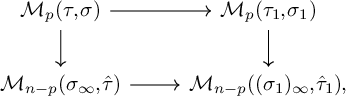
where the horizontal maps are the cosheaf maps. The same is true after tensoring with a commutative ring A.
Proof. Recall that $(\tau , \sigma ) \in \mathcal {J}^S(T^\circ ,T)$
implies that
$(\tau , \sigma ) \in \mathcal {J}^S(T^\circ ,T)$
implies that $\tau \in \partial T^\circ $
and
$\tau \in \partial T^\circ $
and $0 \in \sigma $
. We will use the following essential properties of the contraction operator. First of all, it satisfies the Leibniz property; that is, for any vector v and forms
$0 \in \sigma $
. We will use the following essential properties of the contraction operator. First of all, it satisfies the Leibniz property; that is, for any vector v and forms $\alpha $
and
$\alpha $
and $\beta $
, we have
$\beta $
, we have
 $$\begin{align*}\iota_{v}(\alpha \wedge \beta) = (\iota_v \alpha) \wedge \beta + (-1)^{\deg \alpha} \alpha \wedge (\iota_v \beta).\end{align*}$$
Next, for any vector $v \in N$
, we have
$v \in N$
, we have
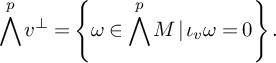 $$ \begin{align} \bigwedge^p v^{\perp} = \left \{ \omega \in \bigwedge^p M\, | \, \iota_v \omega = 0 \right \}. \end{align} $$
Let us first prove that the map is well defined. Notice that
 $$\begin{align*}\iota_v (\iota_{v \wedge z} \Omega_N) = 0. \end{align*}$$
In particular, $ \iota _{v \wedge z} \Omega _N \in \bigwedge ^{n-p} v^{\perp }$
. Since v is a vertex of
$ \iota _{v \wedge z} \Omega _N \in \bigwedge ^{n-p} v^{\perp }$
. Since v is a vertex of $\tau $
, it is also tangent to a one-dimensional edge of
$\tau $
, it is also tangent to a one-dimensional edge of $\hat \tau $
. This proves that
$\hat \tau $
. This proves that
 $$\begin{align*}\iota_{v \wedge z} \Omega_N \in \mathcal F_{n-p}(0, \hat \tau). \end{align*}$$
Now let $z \in \langle C(\tau ) \rangle \wedge \mathcal {F}_{p-1}(0,\sigma _{\infty })$
. We need to show that
$z \in \langle C(\tau ) \rangle \wedge \mathcal {F}_{p-1}(0,\sigma _{\infty })$
. We need to show that $ \iota _{v \wedge z} \Omega _N \in \langle C(\sigma ) \rangle \wedge \mathcal {F}_{n-p-1}(0,\tau )$
. Let
$ \iota _{v \wedge z} \Omega _N \in \langle C(\sigma ) \rangle \wedge \mathcal {F}_{n-p-1}(0,\tau )$
. Let $f_1, \ldots , f_q \in M$
be the vertices of
$f_1, \ldots , f_q \in M$
be the vertices of $\sigma _{\infty }$
. We can complete them to form an oriented basis
$\sigma _{\infty }$
. We can complete them to form an oriented basis $\{f_1, \ldots , f_{n+1} \}$
of M, so that
$\{f_1, \ldots , f_{n+1} \}$
of M, so that
 $$\begin{align*}\Omega_N = f_1 \wedge \ldots \wedge f_{n+1}. \end{align*}$$
We denote by $\{f_1^*, \ldots , f_{n+1}^* \}$
the dual basis of N. For every multi-index
$\{f_1^*, \ldots , f_{n+1}^* \}$
the dual basis of N. For every multi-index $I =(i_1, \ldots , i_p)$
, define the following sign:
$I =(i_1, \ldots , i_p)$
, define the following sign:
 $$\begin{align*}(-1)^{I} := \prod_{k \in I} (-1)^{k+1}. \end{align*}$$
Let $e_1, \ldots , e_s \in N$
be the vertices of
$e_1, \ldots , e_s \in N$
be the vertices of $\tau $
. We can assume
$\tau $
. We can assume
 $$\begin{align*}v = e_1. \end{align*}$$
Since $\sigma _\infty \subset \min (C(\tau ))^\vee $
and by reflexivity, we have
$\sigma _\infty \subset \min (C(\tau ))^\vee $
and by reflexivity, we have
 $$ \begin{align} \langle f_i, e_j\rangle = 1 \quad \text{for all} \ \ 1\leq i \leq q \ \text{and} \ 1 \leq j \leq s. \end{align} $$
By definition,
 $$\begin{align*}\mathcal F_p(0 , \sigma_{\infty})=\sum_{1 \leq i <j \leq q} \bigwedge^p (f_i - f_j)^\perp. \end{align*}$$
Without loss of generality, we can consider
 $$\begin{align*}\omega \in \bigwedge^{p-1} (f_1 - f_2)^\perp \end{align*}$$
and let
 $$\begin{align*}z = e_2 \wedge \omega. \end{align*}$$
Then $z \in \langle C(\tau ) \rangle \wedge \mathcal {F}_{p-1}(0,\sigma _{\infty })$
. Observe that
$z \in \langle C(\tau ) \rangle \wedge \mathcal {F}_{p-1}(0,\sigma _{\infty })$
. Observe that
 $$\begin{align*}(f_1 - f_2)^\perp = \langle f_1^* + f_2^*, f_3^*, \ldots, f_{n+1}^* \rangle.\end{align*}$$
Therefore, by linearity, it is enough to consider two cases for $\omega $
: either
$\omega $
: either $\omega = f^*_I$
, with
$\omega = f^*_I$
, with $I=\{i_1, \ldots , i_{p-1} \} \subset \{3, \ldots , n+1 \}$
, or
$I=\{i_1, \ldots , i_{p-1} \} \subset \{3, \ldots , n+1 \}$
, or $\omega = (f_1^* + f_2^*) \wedge f_I^*$
, with
$\omega = (f_1^* + f_2^*) \wedge f_I^*$
, with $I=\{i_1, \ldots , i_{p-2} \} \subset \{3, \ldots , n+1 \}$
. In these two cases, we compute
$I=\{i_1, \ldots , i_{p-2} \} \subset \{3, \ldots , n+1 \}$
. In these two cases, we compute $\iota _{e_1 \wedge z} \Omega _N = \iota _{e_1 \wedge e_2 \wedge \omega } \Omega _N$
. In the first case, we have
$\iota _{e_1 \wedge z} \Omega _N = \iota _{e_1 \wedge e_2 \wedge \omega } \Omega _N$
. In the first case, we have
 $$\begin{align*}\iota_{e_1 \wedge e_2 \wedge \omega} \Omega_N = \iota_{e_1}( \iota_{e_2} (\iota _{f_I^*} \Omega_N )) = (-1)^I \iota_{e_1}( \iota_{e_2} (f_1 \wedge f_2 \wedge f_{I'} )), \end{align*}$$
where $I'$
is the complement of I in
$I'$
is the complement of I in $\{3, \ldots , n+1\}$
. Using the Leibnitz rule for
$\{3, \ldots , n+1\}$
. Using the Leibnitz rule for $\iota $
and relations (22), we compute that
$\iota $
and relations (22), we compute that
 $$\begin{align*}\begin{aligned} \ & \iota_{e_1}( \iota_{e_2} (f_1 \wedge f_2 \wedge f_{I'} )) = \iota_{e_1}((f_2 - f_1) \wedge f_{I'} +f_1 \wedge f_2 \wedge (\iota_{e_2} f_{I'})) = \\ \ &=(f_1 - f_2) \wedge (\iota_{e_1} f_{I'}) + (f_2 - f_1) \wedge (\iota_{e_2} f_{I'}) + f_1 \wedge f_2 \wedge (\iota_{e_1 \wedge e_2} f_{I'})) = \\ \ &= (f_1 - f_2) \wedge (\iota_{e_1-e_2} f_{I'}) + f_1 \wedge f_2 \wedge (\iota_{e_1 \wedge e_2} f_{I'}). \end{aligned} \end{align*}$$
We now have that $f_1$
and
$f_1$
and $f_1 - f_2$
are both in
$f_1 - f_2$
are both in $C(\sigma )$
and
$C(\sigma )$
and $\iota _{e_1-e_2} f_{I'} \in \bigwedge ^{n-p-1} (e_1 - e_2)^{\perp }$
by (21). In particular, since
$\iota _{e_1-e_2} f_{I'} \in \bigwedge ^{n-p-1} (e_1 - e_2)^{\perp }$
by (21). In particular, since $e_1 - e_2$
is tangent to a one-dimensional edge of
$e_1 - e_2$
is tangent to a one-dimensional edge of $\tau $
, we have
$\tau $
, we have $\iota _{e_1-e_2} f_{I'} \in \mathcal F_{n-p-1}(0, \tau )$
. Now observe that
$\iota _{e_1-e_2} f_{I'} \in \mathcal F_{n-p-1}(0, \tau )$
. Now observe that
 $$\begin{align*}\iota_{e_1 - e_2} (f_2 \wedge (\iota_{e_1 \wedge e_2} f_{I'})) = \iota_{e_1 - e_2} (f_2 \wedge (\iota_{(e_1 - e_2)\wedge e_2} f_{I'})) = 0, \end{align*}$$
so that also $f_2 \wedge (\iota _{e_1 \wedge e_2} f_{I'}) \in \mathcal F_{n-p-1}(0, \tau ) $
. Hence, this proves, for this case, that
$f_2 \wedge (\iota _{e_1 \wedge e_2} f_{I'}) \in \mathcal F_{n-p-1}(0, \tau ) $
. Hence, this proves, for this case, that $\iota _{v \wedge z} \Omega _N \in \langle C(\sigma ) \rangle \wedge \mathcal {F}_{n-p-1}(0,\tau )$
.
$\iota _{v \wedge z} \Omega _N \in \langle C(\sigma ) \rangle \wedge \mathcal {F}_{n-p-1}(0,\tau )$
.
In the second case (i.e., $\omega = (f_1^* + f_2^*) \wedge f_I^*$
), a similar computation shows that
$\omega = (f_1^* + f_2^*) \wedge f_I^*$
), a similar computation shows that
 $$\begin{align*}\iota_{e_1 \wedge e_2 \wedge \omega} \Omega_N = (-1)^I(f_2 - f_1) \wedge (\iota_{e_1 \wedge e_2} f_{I'}). \end{align*}$$
Again, also in this case, $\iota _{v \wedge z} \Omega _N \in \langle C(\sigma ) \rangle \wedge \mathcal {F}_{n-p-1}(0,\tau )$
. This concludes the proof that (20) is well defined.
$\iota _{v \wedge z} \Omega _N \in \langle C(\sigma ) \rangle \wedge \mathcal {F}_{n-p-1}(0,\tau )$
. This concludes the proof that (20) is well defined.
Now consider two different vertices of $\tau $
, v and
$\tau $
, v and $v'$
. We prove that
$v'$
. We prove that $\iota _{v \wedge z}\Omega _N - \iota _{v' \wedge z} \Omega _N$
is in
$\iota _{v \wedge z}\Omega _N - \iota _{v' \wedge z} \Omega _N$
is in $\langle C(\sigma ) \rangle \wedge \mathcal {F}_{n-p-1}(0,\tau )$
. This would show that the map (20) is independent of v. It is enough to check this for
$\langle C(\sigma ) \rangle \wedge \mathcal {F}_{n-p-1}(0,\tau )$
. This would show that the map (20) is independent of v. It is enough to check this for $z \in \bigwedge ^p f_1^{\perp }$
. In particular, we can assume
$z \in \bigwedge ^p f_1^{\perp }$
. In particular, we can assume $z = f_{I}^*$
for some multi-index such that
$z = f_{I}^*$
for some multi-index such that $1 \notin I$
. Then
$1 \notin I$
. Then
 $$\begin{align*}\begin{aligned} \iota_{v \wedge z}\Omega_N - \iota_{v' \wedge z} \Omega_N & = \iota_{v-v'} ( \iota_{f^*_I} \Omega_N) = (-1)^I \iota_{v-v'} (f_1 \wedge f_{I'}) = - (-1)^If_1 \wedge (\iota_{v-v'} (f_{I'})) \end{aligned} \end{align*}$$
for some multi-index $I'$
such that
$I'$
such that $1 \notin I'$
. Now we have
$1 \notin I'$
. Now we have $f_1 \in \langle C(\sigma ) \rangle $
and
$f_1 \in \langle C(\sigma ) \rangle $
and $\iota _{v-v'} (f_{I'}) \in \bigwedge ^{n-p-1} (v-v')^\perp \subseteq \mathcal F_{n-p-1}(0, \tau )$
. Hence,
$\iota _{v-v'} (f_{I'}) \in \bigwedge ^{n-p-1} (v-v')^\perp \subseteq \mathcal F_{n-p-1}(0, \tau )$
. Hence, $\iota _{v \wedge z}\Omega _N - \iota _{v' \wedge z} \Omega _N \in \langle C(\sigma ) \rangle \wedge \mathcal {F}_{n-p-1}(0,\tau )$
.
$\iota _{v \wedge z}\Omega _N - \iota _{v' \wedge z} \Omega _N \in \langle C(\sigma ) \rangle \wedge \mathcal {F}_{n-p-1}(0,\tau )$
.
We now prove that (20) is invertible. In fact, consider the same map,but in the opposite direction $\mathcal M_{n-p}(\sigma _\infty , \hat {\tau }) \rightarrow \mathcal M_p(\tau ,\sigma )$
, using a vertex w of
$\mathcal M_{n-p}(\sigma _\infty , \hat {\tau }) \rightarrow \mathcal M_p(\tau ,\sigma )$
, using a vertex w of $\sigma _{\infty }$
(instead of v) and the
$\sigma _{\infty }$
(instead of v) and the $(n+1)$
-form
$(n+1)$
-form $\Omega _M\in \bigwedge ^{n+1} N$
. This map (up to a sign) is the inverse of (20). Indeed, we prove that
$\Omega _M\in \bigwedge ^{n+1} N$
. This map (up to a sign) is the inverse of (20). Indeed, we prove that
 $$\begin{align*}[\iota_{w \wedge (\iota_{v \wedge z} \Omega_{N})} \Omega_M] = \epsilon [z], \end{align*}$$
where $\epsilon = (-1)^{\tfrac {n(n+5)}{2}}$
.
$\epsilon = (-1)^{\tfrac {n(n+5)}{2}}$
.
It is enough to consider $z \in \bigwedge ^{p} f_1^{\perp }$
; in particular, we can assume
$z \in \bigwedge ^{p} f_1^{\perp }$
; in particular, we can assume
 $$\begin{align*}z = f_I^{*}, \end{align*}$$
where I is some multi-index with $1 \notin I$
and
$1 \notin I$
and $|I| = p$
. Then
$|I| = p$
. Then
 $$\begin{align*}\iota_{v \wedge z} \Omega_{N} = (-1)^{I} \iota_v(f_1 \wedge f_{I'}) = (-1)^I (f_{I'} - f_1 \wedge (\iota_v f_{I'})),\end{align*}$$
where $I'$
is the complement of I in
$I'$
is the complement of I in $\{ 2, \ldots , n+1 \}$
. We can assume that the vertex w of
$\{ 2, \ldots , n+1 \}$
. We can assume that the vertex w of $\sigma _{\infty }$
is
$\sigma _{\infty }$
is $f_1$
. Hence,
$f_1$
. Hence,
 $$\begin{align*}w \wedge (\iota_{v \wedge z} \Omega_{N}) = (-1)^I f_1 \wedge f_{I'}. \end{align*}$$
We have
 $$\begin{align*}\Omega_M = f_1^* \wedge \ldots \wedge f_{n+1}^*. \end{align*}$$
Therefore,
 $$\begin{align*}\iota_{w \wedge (\iota_{v \wedge z} \Omega_{N})} \Omega_M = (-1)^I \iota_{f_1 \wedge f_{I'}} \Omega_M = (-1)^I (-1)^{I'} f_{I}^* = (-1)^I (-1)^{I'} z. \end{align*}$$
Since $I \cup I' = \{2, \ldots , n+1 \}$
, it is easy to show that
$I \cup I' = \{2, \ldots , n+1 \}$
, it is easy to show that $ (-1)^I (-1)^{I'} = (-1)^{\tfrac {n(n+5)}{2}}$
. This concludes the proof that (20) is an isomorphism.
$ (-1)^I (-1)^{I'} = (-1)^{\tfrac {n(n+5)}{2}}$
. This concludes the proof that (20) is an isomorphism.
Let us prove the compatibility with cosheaf maps. We have an inclusion $(\tau _1, \sigma _1) \hookrightarrow (\tau , \sigma )$
if and only if
$(\tau _1, \sigma _1) \hookrightarrow (\tau , \sigma )$
if and only if $\tau \subset \tau _1$
and
$\tau \subset \tau _1$
and $\sigma \subset \sigma _1$
. In particular, in defining (20), the vertex v of
$\sigma \subset \sigma _1$
. In particular, in defining (20), the vertex v of $\tau $
is also a vertex of
$\tau $
is also a vertex of $\tau _1$
. Moreover, the coheaf maps
$\tau _1$
. Moreover, the coheaf maps $\mathcal F_p(0, \sigma ) \rightarrow \mathcal F_p(0, \sigma _1)$
and
$\mathcal F_p(0, \sigma ) \rightarrow \mathcal F_p(0, \sigma _1)$
and $\mathcal F_{n-p}(0, \hat \tau ) \rightarrow \mathcal F_{n-p}(0, \hat \tau _1)$
are just inclusions of sub-modules. So that we have a commuting diagram:
$\mathcal F_{n-p}(0, \hat \tau ) \rightarrow \mathcal F_{n-p}(0, \hat \tau _1)$
are just inclusions of sub-modules. So that we have a commuting diagram:
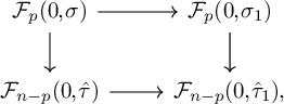
where the vertical arrows are given by the map $z \mapsto \iota _{v \wedge z} \Omega _N$
. When we pass to the quotients, we get the commuting diagram in the statement of the theorem.
$z \mapsto \iota _{v \wedge z} \Omega _N$
. When we pass to the quotients, we get the commuting diagram in the statement of the theorem.
In particular, this proves that the pairs $(\mathcal {J}^S(T^\circ ,T), \mathcal M_p \otimes A)$
and
$(\mathcal {J}^S(T^\circ ,T), \mathcal M_p \otimes A)$
and $( \mathcal {J}^S(T, T^\circ ) , \mathcal M_{n-p} \otimes A)$
are canonically isomorphic, and therefore, they have canonically isomorphic homologies. This concludes the proof.
$( \mathcal {J}^S(T, T^\circ ) , \mathcal M_{n-p} \otimes A)$
are canonically isomorphic, and therefore, they have canonically isomorphic homologies. This concludes the proof.
4 Patchworking and mirror symmetry
We now consider real Calabi-Yau hypersurfaces coming from combinatorial patchworking. We will use Theorem 3.7 in order to give a necessary and sufficient condition for such real Calabi-Yau to be connected.
4.1 Combinatorial patchworking
The patchworking method was invented by Viro in the 1980s, and it has proved to be a very powerful tool to construct real algebraic hypersurfaces (and complete intersections) in toric varieties with prescribed topology of the real part [Reference Viro22], [Reference Viro21]. Let us recall here the (primitive) combinatorial version. Let $\Delta $
be a lattice polytope in
$\Delta $
be a lattice polytope in $M_{\mathbb {R}}$
and T a primitive lattice triangulation of
$M_{\mathbb {R}}$
and T a primitive lattice triangulation of $\Delta $
. Let
$\Delta $
. Let $\varepsilon :\Delta \cap M\rightarrow \mathbb {F}_2$
be a sign distribution on the lattice points of
$\varepsilon :\Delta \cap M\rightarrow \mathbb {F}_2$
be a sign distribution on the lattice points of $\Delta $
(since the triangulation is primitive, note that the lattice points of
$\Delta $
(since the triangulation is primitive, note that the lattice points of $\Delta $
coincide with the vertices of the triangulation). When we say signs in the context of Viro’s patchworking, we will identify
$\Delta $
coincide with the vertices of the triangulation). When we say signs in the context of Viro’s patchworking, we will identify $+$
with
$+$
with $0\in \mathbb {F}_2$
and
$0\in \mathbb {F}_2$
and $-$
with
$-$
with $1$
.
$1$
.
Recall that the real part of the toric variety associated to $\Sigma _\Delta $
is constructed by considering a certain quotient of copies
$\Sigma _\Delta $
is constructed by considering a certain quotient of copies $\Delta (\xi )$
of
$\Delta (\xi )$
of $\Delta $
for any group homomophism
$\Delta $
for any group homomophism $\xi :M \rightarrow \mathbb {F}_2$
; see Equation (3). Denote by
$\xi :M \rightarrow \mathbb {F}_2$
; see Equation (3). Denote by $T(\xi )$
the triangulation of
$T(\xi )$
the triangulation of $\Delta (\xi )$
induced by T. Given a lattice point
$\Delta (\xi )$
induced by T. Given a lattice point $v\in \Delta $
, the sign of its copy
$v\in \Delta $
, the sign of its copy $v(\xi )$
in
$v(\xi )$
in $\Delta (\xi )$
is defined by
$\Delta (\xi )$
is defined by $\varepsilon (v(\xi )) = \xi (v)+\varepsilon (v) \in \mathbb {F}_2$
. For any
$\varepsilon (v(\xi )) = \xi (v)+\varepsilon (v) \in \mathbb {F}_2$
. For any $\xi $
and any
$\xi $
and any $(n+1)$
-simplex
$(n+1)$
-simplex $\sigma $
of
$\sigma $
of $\Delta (\xi )$
, separate the vertices having different signs by taking the union of convex hulls of barycenters of simplices
$\Delta (\xi )$
, separate the vertices having different signs by taking the union of convex hulls of barycenters of simplices $\sigma _1\subset \cdots \subset \sigma $
such that
$\sigma _1\subset \cdots \subset \sigma $
such that $\sigma _1$
is an edge with different signs. This gives a simplicial complex defining a PL-hypersurface in the quotient
$\sigma _1$
is an edge with different signs. This gives a simplicial complex defining a PL-hypersurface in the quotient $\mathbb {R}\Sigma _\Delta $
, denoted by
$\mathbb {R}\Sigma _\Delta $
, denoted by $X_{T,\varepsilon }$
. See Figures 5 and 8 for examples (ignore the divisors for the moment). In the standard description of combinatorial patchworking [Reference Itenberg17], the hypersurface
$X_{T,\varepsilon }$
. See Figures 5 and 8 for examples (ignore the divisors for the moment). In the standard description of combinatorial patchworking [Reference Itenberg17], the hypersurface $X_{T,\varepsilon }$
is defined by considering convex hulls of midpoints of edges with different signs, but the two descriptions give the same result up to isotopy. In the case of a convex triangulation induced by a convex function
$X_{T,\varepsilon }$
is defined by considering convex hulls of midpoints of edges with different signs, but the two descriptions give the same result up to isotopy. In the case of a convex triangulation induced by a convex function $\mu : \Delta \rightarrow \mathbb {R}$
, Viro’s combinatorial patchworking theorem states that the PL-hypersurface
$\mu : \Delta \rightarrow \mathbb {R}$
, Viro’s combinatorial patchworking theorem states that the PL-hypersurface $X_{T,\varepsilon }$
is ambient isotopic (in
$X_{T,\varepsilon }$
is ambient isotopic (in $\mathbb {R}\Sigma _\Delta $
) to the closure (in
$\mathbb {R}\Sigma _\Delta $
) to the closure (in $\mathbb {R}\Sigma _\Delta $
) of the hypersurface in
$\mathbb {R}\Sigma _\Delta $
) of the hypersurface in $(\mathbb {R}^*)^{n+1}$
defined by the polynomial
$(\mathbb {R}^*)^{n+1}$
defined by the polynomial
 $$ \begin{align} \sum_{v\in \Delta\cap M} (-1)^{\varepsilon(v)} t^{\mu(v)} x^v, \end{align} $$
for t small enough and positive. In this text, we consider also different compactifications. In fact, given primitive central triangulations $T^{\circ }$
and T of a pair of dual reflexive polytopes
$T^{\circ }$
and T of a pair of dual reflexive polytopes $\Delta ^{\circ }$
and
$\Delta ^{\circ }$
and $\Delta $
, we consider the toric variety coming from the fan
$\Delta $
, we consider the toric variety coming from the fan $\Sigma _{T^\circ }$
. We denote by
$\Sigma _{T^\circ }$
. We denote by $X_{T^\circ ,T,\varepsilon }$
the compactification of
$X_{T^\circ ,T,\varepsilon }$
the compactification of $X_{T,\varepsilon }\cap (\mathbb {R}^*)^{n+1}$
in
$X_{T,\varepsilon }\cap (\mathbb {R}^*)^{n+1}$
in $\mathbb {R}\Sigma _{T^\circ }$
. Again, under convexity hypothesis, the PL-hypersurface
$\mathbb {R}\Sigma _{T^\circ }$
. Again, under convexity hypothesis, the PL-hypersurface $X_{T^\circ ,T,\varepsilon }$
is ambient isotopic in
$X_{T^\circ ,T,\varepsilon }$
is ambient isotopic in $\mathbb {R}\Sigma _{T^\circ }$
to the compactification in
$\mathbb {R}\Sigma _{T^\circ }$
to the compactification in $\mathbb {R}\Sigma _{T^\circ }$
of the hypersurface given by (23).
$\mathbb {R}\Sigma _{T^\circ }$
of the hypersurface given by (23).
4.2 Patchworking and divisors in the mirror
Consider the Picard group of a toric variety $\mathbb {C}\Sigma $
with
$\mathbb {C}\Sigma $
with $\mathbb {F}_{2}$
coefficients, denoted by
$\mathbb {F}_{2}$
coefficients, denoted by $\operatorname {\mathrm {Pic}}_{\mathbb {F}_2}(\mathbb {C}\Sigma )$
. For a smooth toric variety
$\operatorname {\mathrm {Pic}}_{\mathbb {F}_2}(\mathbb {C}\Sigma )$
. For a smooth toric variety $\mathbb {C}\Sigma $
with
$\mathbb {C}\Sigma $
with $\Sigma $
a complete fan in M, this group is computed as follows. Let
$\Sigma $
a complete fan in M, this group is computed as follows. Let $\operatorname {\mathrm {Div}}_{\text {toric}} \mathbb {C}\Sigma $
be the free module generated by toric divisors; that is,
$\operatorname {\mathrm {Div}}_{\text {toric}} \mathbb {C}\Sigma $
be the free module generated by toric divisors; that is,
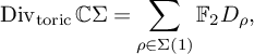 $$\begin{align*}\operatorname{\mathrm{Div}}_{\text{toric}} \mathbb{C}\Sigma = \sum_{\rho \in \Sigma(1)} \mathbb{F}_{2} D_{\rho}, \end{align*}$$
where the sum runs over all rays of the fan (i.e., one-dimensional cones) and $D_{\rho }$
is the toric divisor associated to the ray. Then we have the following short exact sequence:
$D_{\rho }$
is the toric divisor associated to the ray. Then we have the following short exact sequence:
 $$ \begin{align} 0 \rightarrow N \otimes \mathbb{F}_2 \rightarrow \operatorname{\mathrm{Div}}_{\text{toric}} \mathbb{C}\Sigma \rightarrow \operatorname{\mathrm{Pic}}_{\mathbb{F}_2}(\mathbb{C}\Sigma) \rightarrow 0. \end{align} $$
The second arrow is the map $n \mapsto \sum _{\rho } \langle n,v_{\rho } \rangle D_{\rho }$
, where
$n \mapsto \sum _{\rho } \langle n,v_{\rho } \rangle D_{\rho }$
, where $v_{\rho } \in M \otimes \mathbb {F}_{2}$
is the
$v_{\rho } \in M \otimes \mathbb {F}_{2}$
is the $\mod 2$
reduction of the primitive generator of the ray
$\mod 2$
reduction of the primitive generator of the ray $\rho $
, see [Reference Fulton13] and [Reference Cox, Little and Schenck11].
$\rho $
, see [Reference Fulton13] and [Reference Cox, Little and Schenck11].
We now go back to the dual reflexive polytopes $\Delta $
and
$\Delta $
and $\Delta ^{\circ }$
with primitive central triangulations T and
$\Delta ^{\circ }$
with primitive central triangulations T and $T^{\circ }$
. Suppose we do patchworking with T and some sign distribution
$T^{\circ }$
. Suppose we do patchworking with T and some sign distribution $\varepsilon $
, thus obtaining a PL-hypersurface
$\varepsilon $
, thus obtaining a PL-hypersurface $X_{T^{\circ }, T,\varepsilon }$
in
$X_{T^{\circ }, T,\varepsilon }$
in $\mathbb {R}\Sigma _{T^\circ }$
, which, in the convex case, is isotopic to a real Calabi-Yau variety.
$\mathbb {R}\Sigma _{T^\circ }$
, which, in the convex case, is isotopic to a real Calabi-Yau variety.
The sign distribution $\varepsilon $
also determines a toric divisor
$\varepsilon $
also determines a toric divisor $D^{\varepsilon } \in \operatorname {\mathrm {Div}}_{\text {toric}} \mathbb {C}\Sigma _T $
as follows. Let
$D^{\varepsilon } \in \operatorname {\mathrm {Div}}_{\text {toric}} \mathbb {C}\Sigma _T $
as follows. Let $\mathbf {o} \in T$
be the unique interior lattice point. Then the other lattice points
$\mathbf {o} \in T$
be the unique interior lattice point. Then the other lattice points $v \in \partial T$
are the primitive generators of the rays of the fan
$v \in \partial T$
are the primitive generators of the rays of the fan $\Sigma _T$
. Therefore, we can define
$\Sigma _T$
. Therefore, we can define
 $$\begin{align*}D^{\varepsilon} = \sum_{\varepsilon(v) = \varepsilon (\mathbf o)} D_{v}. \end{align*}$$
It is clear that, up to inverting the sign of every lattice point in T, there is a one to one correspondence between toric divisors with $\mathbb {F}_2$
coefficients on
$\mathbb {F}_2$
coefficients on $\mathbb {C}\Sigma _T$
and a choice of patchworking signs on T. Therefore, we denote by
$\mathbb {C}\Sigma _T$
and a choice of patchworking signs on T. Therefore, we denote by $X_{T^{\circ }, T, D}$
the PL-hypersurface in
$X_{T^{\circ }, T, D}$
the PL-hypersurface in $\mathbb {R}\Sigma _{T^{\circ }}$
constructed by the patchworking signs determined by
$\mathbb {R}\Sigma _{T^{\circ }}$
constructed by the patchworking signs determined by $D \in \operatorname {\mathrm {Div}}_{\text {toric}} \mathbb {C}\Sigma _T$
. We have then the following:
$D \in \operatorname {\mathrm {Div}}_{\text {toric}} \mathbb {C}\Sigma _T$
. We have then the following:
Proposition 4.1. If two divisors D and $D'$
in
$D'$
in $\operatorname {\mathrm {Div}}_{\text {toric}} \mathbb {C}\Sigma _T$
define the same class in
$\operatorname {\mathrm {Div}}_{\text {toric}} \mathbb {C}\Sigma _T$
define the same class in $\operatorname {\mathrm {Pic}}_{\mathbb {F}_2}(\mathbb {C}\Sigma _T)$
, then
$\operatorname {\mathrm {Pic}}_{\mathbb {F}_2}(\mathbb {C}\Sigma _T)$
, then $X_{T^{\circ }, T, D}$
and
$X_{T^{\circ }, T, D}$
and $X_{T^{\circ }, T, D'}$
coincide, up to an automorphism of
$X_{T^{\circ }, T, D'}$
coincide, up to an automorphism of $\mathbb {R}\Sigma _{T^{\circ }}$
.
$\mathbb {R}\Sigma _{T^{\circ }}$
.
Proof. We will prove that D and $D'$
are equivalent
$D'$
are equivalent $\mathbb {F}_2$
divisors if and only if they correspond to sign distributions
$\mathbb {F}_2$
divisors if and only if they correspond to sign distributions $\varepsilon $
and
$\varepsilon $
and $\varepsilon '$
satisfying
$\varepsilon '$
satisfying $\varepsilon '=\varepsilon +\xi $
for some
$\varepsilon '=\varepsilon +\xi $
for some $\xi \in \operatorname {\mathrm {Hom}}(M,\mathbb {F}_2)$
. This obviously implies the statement. Using (24), D and
$\xi \in \operatorname {\mathrm {Hom}}(M,\mathbb {F}_2)$
. This obviously implies the statement. Using (24), D and $D'$
are equivalent divisors if and only if
$D'$
are equivalent divisors if and only if
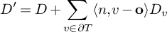 $$\begin{align*}D' = D + \sum_{v \in \partial T} \langle n, v - \mathbf o \rangle D_v \end{align*}$$
for some $n \in N \otimes \mathbb {F}_2$
. Note that
$n \in N \otimes \mathbb {F}_2$
. Note that $N\otimes \mathbb {F}_2=\operatorname {\mathrm {Hom}}(M,\mathbb {F}_2)$
.
$N\otimes \mathbb {F}_2=\operatorname {\mathrm {Hom}}(M,\mathbb {F}_2)$
.
Let
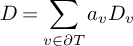 $$\begin{align*}D = \sum_{v \in \partial T} a_v D_v \end{align*}$$
with $a_v \in \mathbb {F}_2$
.
$a_v \in \mathbb {F}_2$
.
Fix the sign of $\mathbf o$
to be
$\mathbf o$
to be $\varepsilon (\mathbf o) = 1\in \mathbb {F}_2$
. Then the signs corresponding to D are
$\varepsilon (\mathbf o) = 1\in \mathbb {F}_2$
. Then the signs corresponding to D are $\varepsilon (v) = a_v$
. Let
$\varepsilon (v) = a_v$
. Let $\xi \in \operatorname {\mathrm {Hom}}(M,\mathbb {F}_2)$
. We see that for
$\xi \in \operatorname {\mathrm {Hom}}(M,\mathbb {F}_2)$
. We see that for $v\in \partial T$
, one has
$v\in \partial T$
, one has
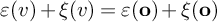 $$ \begin{align*}\varepsilon(v)+\xi (v) = \varepsilon(\mathbf o) + \xi (\mathbf o) \end{align*} $$
iff
 $$ \begin{align*}a_v+\xi (v-\mathbf o)=1. \end{align*} $$
This means that if $\xi = n$
, the divisor corresponding to
$\xi = n$
, the divisor corresponding to $\varepsilon +\xi $
is precisely
$\varepsilon +\xi $
is precisely
 $$ \begin{align*}D + \sum_{v \in \partial T} \langle n, v - \mathbf o \rangle D_v, \end{align*} $$
which is $D'$
. This concludes the proof of the lemma.
$D'$
. This concludes the proof of the lemma.
Example 4.2. The real cubic curves in $\mathbb {P}^2$
obtained from patchworking with the sign distribution corresponding to
$\mathbb {P}^2$
obtained from patchworking with the sign distribution corresponding to $D= D_7 + D_8$
and to
$D= D_7 + D_8$
and to $D=D_8$
are depicted in Figure 5. Notice that the first one is connected, while the second one is not.
$D=D_8$
are depicted in Figure 5. Notice that the first one is connected, while the second one is not.
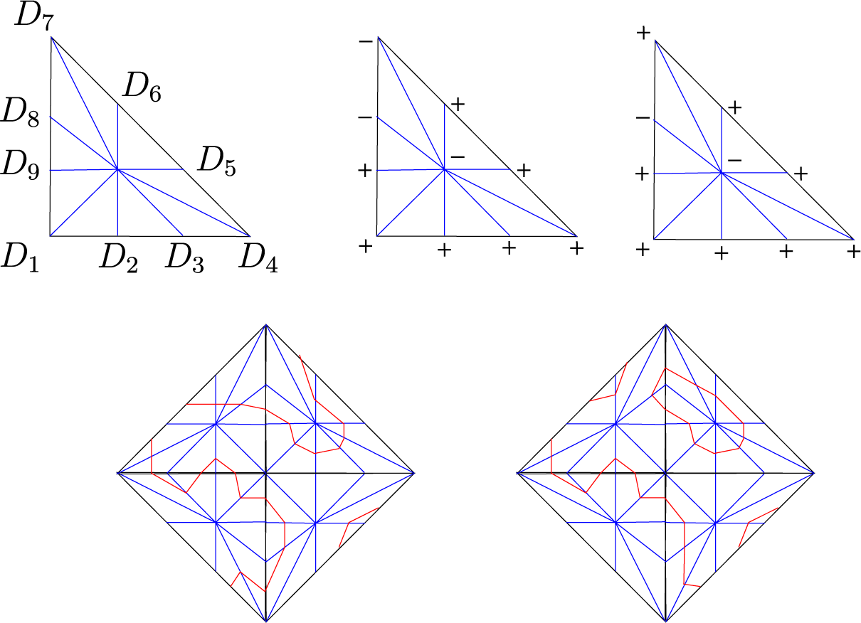
Figure 5 The signs corresponding to $D = D_7 + D_8$
and to
$D = D_7 + D_8$
and to $D=D_8$
and the corresponding real cubics.
$D=D_8$
and the corresponding real cubics.
4.3 Real structures and the patchworking spectral sequence
In this section, we describe in our context the spectral sequence from [Reference Renaudineau and Shaw20], allowing a better understanding of the Betti numbers of a combinatorial patchworking.
Definition 4.3. A real phase structure on $(\Delta , T)$
is the data
$(\Delta , T)$
is the data $\mathcal E$
given by a choice, for every edge
$\mathcal E$
given by a choice, for every edge $\sigma \in T$
, of an element
$\sigma \in T$
, of an element $\mathcal E_{\sigma } \in \frac {N \otimes \mathbb {F}_2}{\sigma ^{\perp }}$
, such that for any two-dimensional simplex
$\mathcal E_{\sigma } \in \frac {N \otimes \mathbb {F}_2}{\sigma ^{\perp }}$
, such that for any two-dimensional simplex $\tau \in T$
, the number of edges
$\tau \in T$
, the number of edges $\sigma $
of
$\sigma $
of $\tau $
such that
$\tau $
such that $\mathcal E_{\sigma } = 0$
is either
$\mathcal E_{\sigma } = 0$
is either $0$
or
$0$
or $2$
.
$2$
.
This definition appeared first in [Reference Renaudineau and Shaw20] for tropical hypersurfaces. Notice that $\mathcal E_{\sigma }$
can also be interpreted as a choice of an affine hyperplane of
$\mathcal E_{\sigma }$
can also be interpreted as a choice of an affine hyperplane of $N \otimes \mathbb {F}_2$
parallel to
$N \otimes \mathbb {F}_2$
parallel to $\sigma ^{\perp }$
. The condition on the two-dimensional simplex
$\sigma ^{\perp }$
. The condition on the two-dimensional simplex $\tau $
is that the three affine hyperplanes, corresponding to the edges of
$\tau $
is that the three affine hyperplanes, corresponding to the edges of $\tau $
, pairwise intersect in three distinct codimension
$\tau $
, pairwise intersect in three distinct codimension $2$
subspaces parallel to
$2$
subspaces parallel to $\tau ^{\perp }$
. A real phase structure is equivalent to a choice of patchworking signs on the triangulation T, up to inversion of all signs. Indeed, this follows by establishing the rule that the vertices of an edge
$\tau ^{\perp }$
. A real phase structure is equivalent to a choice of patchworking signs on the triangulation T, up to inversion of all signs. Indeed, this follows by establishing the rule that the vertices of an edge $\sigma $
have the same sign if and only if
$\sigma $
have the same sign if and only if $\mathcal E_{\sigma }$
is the generator of
$\mathcal E_{\sigma }$
is the generator of $\frac {N \otimes \mathbb {F}_2}{\sigma ^{\perp }}$
. Then a sign distribution determines a real phase structure, and vice versa, given a real phase structure
$\frac {N \otimes \mathbb {F}_2}{\sigma ^{\perp }}$
. Then a sign distribution determines a real phase structure, and vice versa, given a real phase structure $\mathcal E$
, the choice of the sign of one vertex determines the signs of all other vertices.
$\mathcal E$
, the choice of the sign of one vertex determines the signs of all other vertices.
Definition 4.4. Let $\mathcal E$
be a real phase structure on
$\mathcal E$
be a real phase structure on $(\Delta , T)$
. For
$(\Delta , T)$
. For $(\tau ,\sigma )\in \mathcal {P}^1(T^\circ ,T)$
, define
$(\tau ,\sigma )\in \mathcal {P}^1(T^\circ ,T)$
, define
 $$ \begin{align*}\mathcal{E}(\tau,\sigma)=\left\lbrace s\in N\otimes \mathbb{F}_2 / \langle C(\tau) \rangle \:\: \vert \:\: \pi_{\gamma}(s)=\mathcal{E}_\gamma \text{ for some edge } \gamma\subset\sigma \right\rbrace, \end{align*} $$
where $\pi _{\gamma }: N\otimes \mathbb {F}_2 / \langle C(\tau ) \rangle \rightarrow N\otimes \mathbb {F}_2 / \gamma ^\perp $
.
$\pi _{\gamma }: N\otimes \mathbb {F}_2 / \langle C(\tau ) \rangle \rightarrow N\otimes \mathbb {F}_2 / \gamma ^\perp $
.
Define also
 $$ \begin{align*}\mathcal{P}_{\mathbb{R}}(T^\circ,T)= \left\lbrace (\tau, \sigma, s) \:\:\vert \:\: (\tau,\sigma)\in \mathcal{P}(T^\circ,T), s\in N\otimes \mathbb{F}_2 / \langle C(\tau) \rangle \right\rbrace. \end{align*} $$
The set $\mathcal {P}_{\mathbb {R}}(T^\circ ,T)$
is also a poset, where the order is given by
$\mathcal {P}_{\mathbb {R}}(T^\circ ,T)$
is also a poset, where the order is given by $(\tau , \sigma , s)\leq (\tau ', \sigma ', s')$
if
$(\tau , \sigma , s)\leq (\tau ', \sigma ', s')$
if $(\tau , \sigma )\leq _{\mathcal {P}} (\tau ', \sigma ')$
and
$(\tau , \sigma )\leq _{\mathcal {P}} (\tau ', \sigma ')$
and $\pi _{\tau ',\tau }(s')=s$
, where
$\pi _{\tau ',\tau }(s')=s$
, where $\pi _{\tau ',\tau }:N\otimes \mathbb {F}_2 / \langle C(\tau ') \rangle \rightarrow N\otimes \mathbb {F}_2 / \langle C(\tau ) \rangle $
is the
$\pi _{\tau ',\tau }:N\otimes \mathbb {F}_2 / \langle C(\tau ') \rangle \rightarrow N\otimes \mathbb {F}_2 / \langle C(\tau ) \rangle $
is the $\mathbb {F}_2$
reduction of the projection maps (8). Consider the geometric realization of the poset
$\mathbb {F}_2$
reduction of the projection maps (8). Consider the geometric realization of the poset $\mathcal {P}_{\mathbb {R}}(T^\circ ,T)$
and its subdivision given by
$\mathcal {P}_{\mathbb {R}}(T^\circ ,T)$
and its subdivision given by
 $$ \begin{align*}\vert \mathcal{P}_{\mathbb{R}}(T^\circ,T)\vert = \bigcup_{(\tau,\sigma, s)\in \mathcal{P}_{\mathbb{R}}(T^\circ,T)} F(\tau,\sigma,s), \end{align*} $$
where
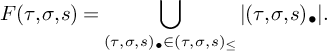 $$ \begin{align*}F(\tau,\sigma,s)= \bigcup_{(\tau,\sigma,s)_\bullet \in (\tau,\sigma,s)_{\leq}}\vert (\tau,\sigma,s)_\bullet \vert. \end{align*} $$
Proposition 4.5. The poset $\mathcal {P}_{\mathbb {R}}(T^\circ ,T)$
is the face poset of a regular CW-structure on
$\mathcal {P}_{\mathbb {R}}(T^\circ ,T)$
is the face poset of a regular CW-structure on $\mathbb {R}\Sigma _{T^\circ }$
with cells
$\mathbb {R}\Sigma _{T^\circ }$
with cells $F(\tau ,\sigma ,s)$
.
$F(\tau ,\sigma ,s)$
.
Proof. This is similar to Proposition 2.7. Here, the face poset of the real toric variety associated to a fan $\Sigma $
is the poset
$\Sigma $
is the poset
 $$ \begin{align*}\Sigma_{\mathbb{R}}:=\left\lbrace (\rho,s) \: \vert \: \rho\in\Sigma \text{ and } s\in N\otimes\mathbb{F}_2 / \langle \rho \rangle \right\rbrace. \end{align*} $$
Again, the poset $\mathcal {P}_{\mathbb {R}}(T^{\circ },T)$
defines a subdivision of
$\mathcal {P}_{\mathbb {R}}(T^{\circ },T)$
defines a subdivision of $\Sigma _{T^\circ ,\mathbb {R}}$
, so their geometric realizations are homeomorphic.
$\Sigma _{T^\circ ,\mathbb {R}}$
, so their geometric realizations are homeomorphic.
Given a real phase structure $\mathcal {E}$
on
$\mathcal {E}$
on $(\Delta ,T)$
, consider the following subposet of
$(\Delta ,T)$
, consider the following subposet of $\mathcal {P}_{\mathbb {R}}(T^{\circ }, T)$
:
$\mathcal {P}_{\mathbb {R}}(T^{\circ }, T)$
:
 $$ \begin{align*}\mathcal{P}^1_{\mathcal{E}}(T^\circ,T)= \left\lbrace (\tau, \sigma, s) \in \mathcal{P}_{\mathbb{R}}(T^\circ,T) \:\: \vert \:\: \dim \sigma \geq 1, \ \ s\in\mathcal{E}(\tau,\sigma) \right\rbrace. \end{align*} $$
Proposition 4.6. Let $\mathcal {E}$
be a real phase structure on
$\mathcal {E}$
be a real phase structure on $(\Delta ,T)$
and let
$(\Delta ,T)$
and let $\varepsilon :\Delta \cap M\rightarrow \mathbb {F}_2$
be a corresponding sign distribution. Then
$\varepsilon :\Delta \cap M\rightarrow \mathbb {F}_2$
be a corresponding sign distribution. Then $\mathcal {P}^1_{\mathcal {E}}(T^\circ ,T)$
is a regular CW-structure on
$\mathcal {P}^1_{\mathcal {E}}(T^\circ ,T)$
is a regular CW-structure on $X_{T^\circ ,T,\varepsilon }$
.
$X_{T^\circ ,T,\varepsilon }$
.
Proof. Recall that the hypersurface $X_{T,\varepsilon }$
is obtained by considering for any
$X_{T,\varepsilon }$
is obtained by considering for any $\xi \in N\otimes \mathbb {F}_2$
and any
$\xi \in N\otimes \mathbb {F}_2$
and any $(n+1)$
-simplex
$(n+1)$
-simplex $\sigma $
of
$\sigma $
of $\Delta (\xi )$
the union of convex hulls of barycenters of simplices
$\Delta (\xi )$
the union of convex hulls of barycenters of simplices $\sigma _1\subset \cdots \subset \sigma $
such that
$\sigma _1\subset \cdots \subset \sigma $
such that $\sigma _1$
is an edge with different signs. So after taking the quotient in
$\sigma _1$
is an edge with different signs. So after taking the quotient in $\mathbb {R}\Sigma _\Delta $
, the hypersurface
$\mathbb {R}\Sigma _\Delta $
, the hypersurface $X_{T,\varepsilon }$
is realized by the poset
$X_{T,\varepsilon }$
is realized by the poset
 $$ \begin{align*}\left\lbrace ((\sigma_1\subset\cdots\subset\sigma_{k}),\xi) \:\: \vert \:\: \sigma_i\in T, \xi\in N\otimes\mathbb{F}_2/(F_k)^\perp, \pi_{\sigma_1}(\xi)=\mathcal{E}_{\sigma_1} \right\rbrace. \end{align*} $$
Here, $F_k$
denotes the minimal face of
$F_k$
denotes the minimal face of $\Delta $
containing
$\Delta $
containing $\sigma _k$
. Recall also that the poset
$\sigma _k$
. Recall also that the poset $\mathcal {P}(T^\circ ,T)$
was defined as a small modification of the poset
$\mathcal {P}(T^\circ ,T)$
was defined as a small modification of the poset
 $$ \begin{align*}\Phi:=\left\lbrace (\rho,\sigma)\in\Sigma_\Delta\times T \mid \sigma\subset \rho^\vee \right\rbrace. \end{align*} $$
One can consider
 $$ \begin{align*}\Phi_{\mathcal{E}}:=\left\lbrace (\rho,\sigma,s) \: \vert \: (\rho,\sigma) \in \Phi \text{ and } s\in \mathcal{E}(\rho,\sigma) \right\rbrace. \end{align*} $$
The surjective map of posets
 $$ \begin{align*}((\sigma_1\subset\cdots\subset\sigma_{k}),\xi)\rightarrow (F_k^\vee,\sigma_1,\xi) \end{align*} $$
shows that $\Phi _{\mathcal {E}}$
induces a regular CW-structure on
$\Phi _{\mathcal {E}}$
induces a regular CW-structure on $X_{T,\varepsilon }$
. The result is obtained by taking the preimages by the map
$X_{T,\varepsilon }$
. The result is obtained by taking the preimages by the map $\operatorname {Bl}: \mathbb {R}\Sigma _{T^\circ } \rightarrow \mathbb {R}\Sigma _{\Delta }$
as in the proof of Proposition 2.7.
$\operatorname {Bl}: \mathbb {R}\Sigma _{T^\circ } \rightarrow \mathbb {R}\Sigma _{\Delta }$
as in the proof of Proposition 2.7.
There is an obvious surjective map from $\mathcal {P}_{\mathbb {R}}(T^\circ ,T)$
to
$\mathcal {P}_{\mathbb {R}}(T^\circ ,T)$
to $\mathcal {P}(T^\circ ,T)$
by forgetting the last coordinate, and results from [Reference Renaudineau and Shaw20] extend to this case. We recall them for reader convenience. The proofs are similar as in [Reference Renaudineau and Shaw20].
$\mathcal {P}(T^\circ ,T)$
by forgetting the last coordinate, and results from [Reference Renaudineau and Shaw20] extend to this case. We recall them for reader convenience. The proofs are similar as in [Reference Renaudineau and Shaw20].
Definition 4.7. The sign cosheaf on $\mathcal {P}(T^\circ ,T)$
is given by
$\mathcal {P}(T^\circ ,T)$
is given by
 $$ \begin{align*}\mathcal{S}(\tau,\sigma):=\mathbb{F}_2^{\mathcal{E}(\tau,\sigma)}. \end{align*} $$
For $\varepsilon \in \mathcal {E}(\tau ,\sigma )$
, we will denote by
$\varepsilon \in \mathcal {E}(\tau ,\sigma )$
, we will denote by $w_\varepsilon $
the corresponding generator of
$w_\varepsilon $
the corresponding generator of $\mathcal {S}(\tau ,\sigma )$
.
$\mathcal {S}(\tau ,\sigma )$
.
Proposition 4.8. For every integer q, the groups $H_q(X_{T^\circ ,T}; \mathcal {S})$
and
$H_q(X_{T^\circ ,T}; \mathcal {S})$
and $H_q(X_{T^\circ ,T,\varepsilon };\mathbb {F}_2)$
are isomorphic.
$H_q(X_{T^\circ ,T,\varepsilon };\mathbb {F}_2)$
are isomorphic.
Proposition 4.9. Let $\mathcal {E}$
be a real phase structure on
$\mathcal {E}$
be a real phase structure on $(\Delta ,T)$
. There exists a filtration of cosheaves on
$(\Delta ,T)$
. There exists a filtration of cosheaves on $\mathcal {P}(T^\circ ,T)$
 $$ \begin{align*}0=\mathcal{K}_{n+1}\subset\mathcal{K}_{n}\subset\mathcal{K}_{n-1}\subset\cdots\subset \mathcal{K}_0=\mathcal{S} \end{align*} $$
such that
 $$ \begin{align*}\mathcal{K}_{p}/\mathcal{K}_{p+1}\simeq \mathcal{F}_p. \end{align*} $$
For the reader’s convenience, we recall briefly the definition of the filtration $\mathcal {K}_p$
and of the isomorphisms
$\mathcal {K}_p$
and of the isomorphisms
 $$ \begin{align*}\mathcal{K}_{p}/\mathcal{K}_{p+1}\simeq \mathcal{F}_p. \end{align*} $$
If $\dim \sigma =1$
, then
$\dim \sigma =1$
, then $\mathcal {E}(\tau ,\sigma )$
is an affine space of direction
$\mathcal {E}(\tau ,\sigma )$
is an affine space of direction $\sigma ^\perp / \langle C(\tau ) \rangle $
. Define in this case
$\sigma ^\perp / \langle C(\tau ) \rangle $
. Define in this case
 $$ \begin{align*}\mathcal{K}_p(\tau,\sigma)=\mathbb{F}_2 \langle \sum_{\varepsilon\in H}w_\varepsilon \:\vert \: H\in \operatorname{\mathrm{Aff}}_p(\mathcal{E}(\tau,\sigma))\rangle,\end{align*} $$
where $\operatorname {\mathrm {Aff}}_p(\mathcal {E}(\tau ,\sigma ))$
is the space of affine subspaces of
$\operatorname {\mathrm {Aff}}_p(\mathcal {E}(\tau ,\sigma ))$
is the space of affine subspaces of $\mathcal {E}(\tau ,\sigma )$
of dimension p. In the general case, consider the sum
$\mathcal {E}(\tau ,\sigma )$
of dimension p. In the general case, consider the sum
 $$ \begin{align*}\mathcal{K}_p(\tau,\sigma):=\sum_{\gamma\subset\sigma \: \dim\gamma=1}\mathcal{K}_p(\tau,\gamma). \end{align*} $$
The isomorphism
 $$ \begin{align*}\mathcal{K}_{p}/\mathcal{K}_{p+1}\simeq \mathcal{F}_p \end{align*} $$
is induced by mapping $w_{G}$
to
$w_{G}$
to $v_1 \wedge \dots \wedge v_p$
, for
$v_1 \wedge \dots \wedge v_p$
, for $G \in \operatorname {\mathrm {Aff}}_p(\mathcal {E}(\tau ,\sigma ))$
where
$G \in \operatorname {\mathrm {Aff}}_p(\mathcal {E}(\tau ,\sigma ))$
where $\dim \sigma =1$
. Here,
$\dim \sigma =1$
. Here, $w_{G}$
denotes
$w_{G}$
denotes $\sum _{\varepsilon \in G}w_\varepsilon $
and
$\sum _{\varepsilon \in G}w_\varepsilon $
and $v_1, \dots , v_p$
form a basis of the tangent space (over
$v_1, \dots , v_p$
form a basis of the tangent space (over $\mathbb {F}_2$
) of G. The spectral sequence
$\mathbb {F}_2$
) of G. The spectral sequence $(E_{p,q}^{k}, \delta ^{[k]})$
associated to this filtration has first page
$(E_{p,q}^{k}, \delta ^{[k]})$
associated to this filtration has first page
 $$ \begin{align*}E^1_{p,q}=H_q(X_{T^\circ,T};\mathcal{F}_p)\end{align*} $$
and converges to $H_\bullet (X_{T^\circ ,T};\mathcal {S})$
, which by Proposition 4.8 is the homology of
$H_\bullet (X_{T^\circ ,T};\mathcal {S})$
, which by Proposition 4.8 is the homology of $X_{T^\circ ,T,\varepsilon }$
.
$X_{T^\circ ,T,\varepsilon }$
.
5 Connectedness
To simplify a little the notations in this section, for a $\mathbb {Z}$
-cosheaf
$\mathbb {Z}$
-cosheaf $\mathcal {G}$
, we will denote by
$\mathcal {G}$
, we will denote by $\mathcal {G}^{\mathbb {F}_2}$
the tensor product
$\mathcal {G}^{\mathbb {F}_2}$
the tensor product $\mathcal {G}\otimes \mathbb {F}_2$
. Let
$\mathcal {G}\otimes \mathbb {F}_2$
. Let $D=\sum _{\rho \in \Sigma _T(1)}a_\rho D_\rho $
be a toric divisor on
$D=\sum _{\rho \in \Sigma _T(1)}a_\rho D_\rho $
be a toric divisor on $\mathbb {C}\Sigma _{T}$
with
$\mathbb {C}\Sigma _{T}$
with $\mathbb {F}_2$
-coefficients. Denote by
$\mathbb {F}_2$
-coefficients. Denote by $\operatorname {\mathrm {supp}}(D)$
the support of D, meaning the set of rays in
$\operatorname {\mathrm {supp}}(D)$
the support of D, meaning the set of rays in $\Sigma _T$
with a non-vanishing coefficient. Again, to simplify the notations, we will identify the ray
$\Sigma _T$
with a non-vanishing coefficient. Again, to simplify the notations, we will identify the ray $\rho $
with the segment
$\rho $
with the segment $S(\rho )$
in T. The divisor D defines, by the same formula, a divisor on
$S(\rho )$
in T. The divisor D defines, by the same formula, a divisor on $\mathbb {T}\Sigma _T$
, and when restricted to
$\mathbb {T}\Sigma _T$
, and when restricted to $X_{T,T^\circ }$
, it defines a class in
$X_{T,T^\circ }$
, it defines a class in $H_{n-1}(X_{T,T^\circ };\mathcal {F}_{n-1}^{\mathbb {F}_2})$
represented by the cycle
$H_{n-1}(X_{T,T^\circ };\mathcal {F}_{n-1}^{\mathbb {F}_2})$
represented by the cycle
 $$ \begin{align*}D_{|X_{T,T^{\circ}}} :=\sum_{ \tiny{\begin{array}{c} \rho\in \operatorname{\mathrm{supp}}(D) \\ \dim(\delta)=1 \text{ and } \delta \subset \min(\rho)^\vee \end{array}}} (\rho,\delta)\otimes v_{\rho,\delta}, \end{align*} $$
where $v_{\rho ,\delta }$
is the generator of
$v_{\rho ,\delta }$
is the generator of $\Lambda _{\mathbb {F}_2}^{n-1}(\frac {\delta ^\perp }{\rho })$
.
$\Lambda _{\mathbb {F}_2}^{n-1}(\frac {\delta ^\perp }{\rho })$
.
Remark 5.1. If T and $T^\circ $
are convex, the Viro polynomial defines the mirror family of complex hypersurfaces
$T^\circ $
are convex, the Viro polynomial defines the mirror family of complex hypersurfaces $X_t^{\circ }$
in
$X_t^{\circ }$
in $\mathbb {C}\Sigma _T$
, and the divisor D restricts to a family of divisors
$\mathbb {C}\Sigma _T$
, and the divisor D restricts to a family of divisors $D_{|X_t^{\circ }}=\sum _{\rho \in \Sigma _T(1)}a_\rho D_\rho \cap X^{\circ }_t$
. Each
$D_{|X_t^{\circ }}=\sum _{\rho \in \Sigma _T(1)}a_\rho D_\rho \cap X^{\circ }_t$
. Each $D_\rho \cap X^{\circ }_t$
when restricted to the toric orbit
$D_\rho \cap X^{\circ }_t$
when restricted to the toric orbit $\mathcal {O}^{\mathbb {C}}_\rho $
defines in turn a Viro polynomial, which is one of the tropical hypersurfaces
$\mathcal {O}^{\mathbb {C}}_\rho $
defines in turn a Viro polynomial, which is one of the tropical hypersurfaces $X_{T,T^\circ }\cap \mathcal {O}^{\mathbb {T}}_\rho $
. The facets of
$X_{T,T^\circ }\cap \mathcal {O}^{\mathbb {T}}_\rho $
. The facets of $X_{T,T^\circ }\cap \mathcal {O}^{\mathbb {T}}_\rho $
are precisely dual to the edges
$X_{T,T^\circ }\cap \mathcal {O}^{\mathbb {T}}_\rho $
are precisely dual to the edges $\delta $
of
$\delta $
of $\Delta ^\circ $
such that
$\Delta ^\circ $
such that $\delta \subset \min (\rho )^\vee $
.
$\delta \subset \min (\rho )^\vee $
.
However, the divisor D also defines a real phase structure $\mathcal {E}=\mathcal {E}^D$
on
$\mathcal {E}=\mathcal {E}^D$
on $(\Delta ,T)$
and a corresponding patchworking
$(\Delta ,T)$
and a corresponding patchworking $X_{T^\circ ,T,\varepsilon }$
. In this section, we will prove the following:
$X_{T^\circ ,T,\varepsilon }$
. In this section, we will prove the following:
Theorem 5.2. Assume that
 $$ \begin{align} H_n(X_{T^\circ,T};\mathcal{F}^{\mathbb{F}_2}_k)=0 \:\: \text{ for all }\:\: 0<k<n. \end{align} $$
Then the patchworking $X_{T^\circ ,T,\varepsilon }$
is connected if and only if
$X_{T^\circ ,T,\varepsilon }$
is connected if and only if $[D_{|X_{T,T^{\circ }}}] \neq 0$
in
$[D_{|X_{T,T^{\circ }}}] \neq 0$
in $H_{n-1}(X_{T,T^\circ };\mathcal {F}_{n-1}^{\mathbb {F}_2})$
.
$H_{n-1}(X_{T,T^\circ };\mathcal {F}_{n-1}^{\mathbb {F}_2})$
.
Remark 5.3. The hypothesis (25) is satisfied if $\Delta $
is a polytope giving rise to a non-singular toric variety. This follows from Proposition 3.2 in [Reference Brugallé, López de Medrano and Rau8] (see also [Reference Arnal, Renaudineau and Shaw2]). We expect that in the convex case, the tropical divisor class
$\Delta $
is a polytope giving rise to a non-singular toric variety. This follows from Proposition 3.2 in [Reference Brugallé, López de Medrano and Rau8] (see also [Reference Arnal, Renaudineau and Shaw2]). We expect that in the convex case, the tropical divisor class $[D_{|X_{T,T^{\circ }}}]$
vanishes in
$[D_{|X_{T,T^{\circ }}}]$
vanishes in $H_{n-1}(X_{\text {trop}}^\circ ;\mathcal {F}_{n-1}^{\mathbb {F}_2})$
if and only if, for t small enough, the class of the complex divisor
$H_{n-1}(X_{\text {trop}}^\circ ;\mathcal {F}_{n-1}^{\mathbb {F}_2})$
if and only if, for t small enough, the class of the complex divisor $[D_{|X^{\circ }_t}]$
vanishes in the Picard group modulo
$[D_{|X^{\circ }_t}]$
vanishes in the Picard group modulo $2$
of
$2$
of $X^{\circ }_t$
.
$X^{\circ }_t$
.
Recall that the real phase structure $\mathcal {E}^D$
defines a sign cosheaf
$\mathcal {E}^D$
defines a sign cosheaf $\mathcal {S}_D$
on
$\mathcal {S}_D$
on $\mathcal {P}(T^\circ ,T)$
and induces a spectral sequence
$\mathcal {P}(T^\circ ,T)$
and induces a spectral sequence $(E^k_{p,q}, \delta ^{[k]})$
converging to
$(E^k_{p,q}, \delta ^{[k]})$
converging to $H_*(X_{T^\circ ,T}; \mathcal {S}_D)$
. Obviously, the spectral sequence depends on D, but to keep notation simple, we remove D from the decorations. In particular, the number of connected components of
$H_*(X_{T^\circ ,T}; \mathcal {S}_D)$
. Obviously, the spectral sequence depends on D, but to keep notation simple, we remove D from the decorations. In particular, the number of connected components of $X_{T^\circ ,T,\varepsilon }$
is given by the dimension of the homology group
$X_{T^\circ ,T,\varepsilon }$
is given by the dimension of the homology group
 $$\begin{align*}H_{n}(X_{T^\circ,T,\varepsilon}, \mathbb{F}_2) \cong \bigoplus_{k} E^{\infty}_{k,n}. \end{align*}$$
Therefore, with assumption (25), the number of connected components of $X_{T^\circ ,T,\varepsilon }$
can be either one or two. If the differential at the first page
$X_{T^\circ ,T,\varepsilon }$
can be either one or two. If the differential at the first page
 $$\begin{align*}\delta^{[1]}: H_n(X_{T^\circ,T}; \mathcal{F}^{\mathbb{F}_2}_0) \rightarrow H_{n-1}(X_{T^\circ,T}; \mathcal{F}^{\mathbb{F}_2}_1) \end{align*}$$
does not vanish (i.e., it is injective), then $X_{T^\circ ,T,\varepsilon }$
is connected. If it vanishes, we need to study also higher differntials
$X_{T^\circ ,T,\varepsilon }$
is connected. If it vanishes, we need to study also higher differntials $\delta ^{[k]}$
. Recall that
$\delta ^{[k]}$
. Recall that $X_{T^\circ , T}$
contains the sphere
$X_{T^\circ , T}$
contains the sphere $S = S_{T^\circ , T}$
(see (7)), and it is homotopically equivalent to it. One direction of Theorem 5.2 follows from the following:
$S = S_{T^\circ , T}$
(see (7)), and it is homotopically equivalent to it. One direction of Theorem 5.2 follows from the following:
Theorem 5.4. Let $S\in H_n(X_{T^\circ ,T}; \mathcal {F}^{\mathbb {F}_2}_0)$
be the generator. Then
$S\in H_n(X_{T^\circ ,T}; \mathcal {F}^{\mathbb {F}_2}_0)$
be the generator. Then $\delta ^{[1]}(S)$
and
$\delta ^{[1]}(S)$
and $[D_{|X_{T,T^{\circ }}}]$
are mirror classes. In particular, if
$[D_{|X_{T,T^{\circ }}}]$
are mirror classes. In particular, if $[D_{|X_{T,T^{\circ }}}] \neq 0$
, then
$[D_{|X_{T,T^{\circ }}}] \neq 0$
, then $X_{T^\circ ,T,\varepsilon }$
is connected.
$X_{T^\circ ,T,\varepsilon }$
is connected.
Proof. We work with the refinement $\mathcal {J}(T^\circ ,T)$
of
$\mathcal {J}(T^\circ ,T)$
of $\mathcal {P}(T^\circ ,T)$
. The generator of
$\mathcal {P}(T^\circ ,T)$
. The generator of $H_n(\mathcal {J}(T^\circ ,T); \mathcal {F}^{\mathbb {F}_2}_0)$
is given by
$H_n(\mathcal {J}(T^\circ ,T); \mathcal {F}^{\mathbb {F}_2}_0)$
is given by
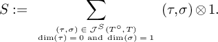 $$ \begin{align*}S:= \sum_{ \tiny{\begin{array}{c} (\tau,\sigma)\in\mathcal{J}^S(T^\circ,T) \\ \dim(\tau)=0 \text{ and } \dim(\sigma)=1 \end{array}}} (\tau,\sigma)\otimes 1. \end{align*} $$
Then a lift of S in $C_n(\mathcal {J}(T^\circ ,T);\mathcal {S}_{D})$
is given by
$C_n(\mathcal {J}(T^\circ ,T);\mathcal {S}_{D})$
is given by $\tilde {S}=S_0+S_1$
with
$\tilde {S}=S_0+S_1$
with
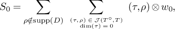 $$ \begin{align*}S_0=\sum_{\rho\notin\text{supp}(D)}\sum_{ \tiny{\begin{array}{c} (\tau,\rho )\in\mathcal{J}(T^\circ,T) \\ \dim(\tau)=0 \end{array}}} (\tau,\rho)\otimes w_{0}, \end{align*} $$
and
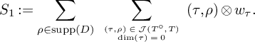 $$ \begin{align*}S_1:=\sum_{\rho\in\text{supp}(D)}\sum_{ \tiny{\begin{array}{c} (\tau, \rho)\in\mathcal{J}(T^\circ,T) \\ \dim(\tau)=0 \end{array}}} (\tau, \rho)\otimes w_{\tau}. \end{align*} $$
The boundary of the chain $\tilde {S}$
in
$\tilde {S}$
in $C_{n-1}(\mathcal {J}(T^\circ ,T);\mathcal {K}_1^D)$
is given by
$C_{n-1}(\mathcal {J}(T^\circ ,T);\mathcal {K}_1^D)$
is given by $A+B$
with
$A+B$
with
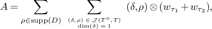 $$ \begin{align*}A=\sum_{\rho\in\text{supp}(D)}\sum_{ \tiny{\begin{array}{c} (\delta, \rho )\in\mathcal{J}(T^\circ,T) \\ \dim(\delta)=1 \end{array}}} (\delta,\rho)\otimes (w_{\tau_1}+w_{\tau_2}), \end{align*} $$
where $\tau _1$
and
$\tau _1$
and $\tau _2$
are the two vertices of
$\tau _2$
are the two vertices of $\delta $
, and
$\delta $
, and
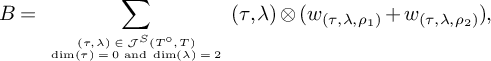 $$ \begin{align*}B=\sum_{ \tiny{\begin{array}{c} (\tau,\lambda)\in\mathcal{J}^S(T^\circ,T) \\ \dim(\tau)=0\text{ and } \dim(\lambda)=2 \end{array}}} (\tau,\lambda)\otimes (w_{(\tau,\lambda,\rho_1)}+w_{(\tau,\lambda,\rho_2)}), \end{align*} $$
where $\rho _1$
and
$\rho _1$
and $\rho _2$
are the two rays of
$\rho _2$
are the two rays of $\Sigma _T$
adjacent to
$\Sigma _T$
adjacent to $C(\lambda )$
, and
$C(\lambda )$
, and
 $$ \begin{align*}w_{(\tau, \lambda,\rho_i)}=\left\lbrace \begin{array}{@{}c} w_0 \text{ if } \rho_i\notin \text{supp}(D), \\ w_{\tau} \text{ if } \rho_i\in \text{supp}(D). \end{array}\right. \end{align*} $$
So finally, the image of S by the map $\delta ^{[1]}$
is represented by
$\delta ^{[1]}$
is represented by $\gamma _1+\gamma _2$
, with
$\gamma _1+\gamma _2$
, with
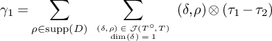 $$\begin{align*}\gamma_1=\sum_{\rho\in\text{supp}(D)}\sum_{ \tiny{\begin{array}{c} (\delta,\rho)\in\mathcal{J}(T^\circ,T) \\ \dim(\delta)=1 \end{array}}} (\delta, \rho)\otimes (\tau_1 - \tau_2) \end{align*}$$
and
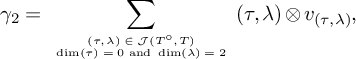 $$ \begin{align*}\gamma_2=\sum_{ \tiny{\begin{array}{c} (\tau,\lambda)\in\mathcal{J}(T^\circ,T) \\ \dim(\tau)=0\text{ and } \dim(\lambda)=2 \end{array}}} (\tau,\lambda)\otimes v_{(\tau,\lambda)}, \end{align*} $$
where $v_{(\tau ,\lambda )}=\tau $
if only one of the two rays of
$v_{(\tau ,\lambda )}=\tau $
if only one of the two rays of $\Sigma _T$
adjacent to
$\Sigma _T$
adjacent to $C(\lambda )$
is contained in the support of D, and is equal to
$C(\lambda )$
is contained in the support of D, and is equal to $0$
otherwise. By definition of the cosheaves
$0$
otherwise. By definition of the cosheaves $\mathcal {M}_p$
, the chain
$\mathcal {M}_p$
, the chain $\gamma _2$
is equal to
$\gamma _2$
is equal to $0$
in
$0$
in $C_{n-1}(\mathcal {J}(T^\circ ,T); \mathcal {M}_1^{\mathbb {F}_2})$
. So in
$C_{n-1}(\mathcal {J}(T^\circ ,T); \mathcal {M}_1^{\mathbb {F}_2})$
. So in $H_{n-1}(\mathcal {J}(T^\circ ,T); \mathcal {M}_1^{\mathbb {F}_2})$
, one has
$H_{n-1}(\mathcal {J}(T^\circ ,T); \mathcal {M}_1^{\mathbb {F}_2})$
, one has
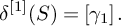 $$ \begin{align*}\delta^{[1]}(S)=\left[\gamma_1\right]. \end{align*} $$
Now, the mirror class of $\left [\gamma _1\right ]$
in
$\left [\gamma _1\right ]$
in $H_{n-1}(\mathcal {J}(T,T^\circ ); \mathcal {M}_{n-1}^{\mathbb {F}_2})$
is given by
$H_{n-1}(\mathcal {J}(T,T^\circ ); \mathcal {M}_{n-1}^{\mathbb {F}_2})$
is given by
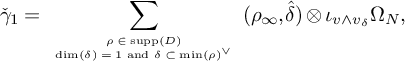 $$ \begin{align*}\check{\gamma}_1= \sum_{ \tiny{\begin{array}{c} \rho\in\text{supp}(D) \\ \dim(\delta)=1 \text{ and } \delta \subset \min(\rho)^\vee \end{array}}} (\rho_\infty,\hat{\delta})\otimes \iota_{v\wedge v_\delta}\Omega_N, \end{align*} $$
where v is a vertex of $\delta $
and we have set
$\delta $
and we have set $v_{\delta } = \tau _1 -\tau _2$
, the direction of
$v_{\delta } = \tau _1 -\tau _2$
, the direction of $\delta $
. Notice that the submodule generated by v and
$\delta $
. Notice that the submodule generated by v and $v_\delta $
is equal to
$v_\delta $
is equal to $\langle \hat {\delta } \rangle $
, and so
$\langle \hat {\delta } \rangle $
, and so $ \iota _{v\wedge v_\delta }\Omega _N$
is the generator of
$ \iota _{v\wedge v_\delta }\Omega _N$
is the generator of $ \Lambda ^{n-1} \langle \hat {\delta } \rangle ^\perp $
. In particular,
$ \Lambda ^{n-1} \langle \hat {\delta } \rangle ^\perp $
. In particular, $ \iota _{v\wedge v_\delta }\Omega _N$
can also be seen as a generator of
$ \iota _{v\wedge v_\delta }\Omega _N$
can also be seen as a generator of $(\mathcal M_{n-1}^{\Delta })^{\mathbb {F}_2}(\rho _{\infty }, \delta )$
. Therefore, as in Example 3.14, the chains
$(\mathcal M_{n-1}^{\Delta })^{\mathbb {F}_2}(\rho _{\infty }, \delta )$
. Therefore, as in Example 3.14, the chains $\check {\gamma }_1$
and
$\check {\gamma }_1$
and $D_{|X_{T,T^{\circ }}}$
are homologous by the following chain in
$D_{|X_{T,T^{\circ }}}$
are homologous by the following chain in $C_{n}(\mathcal {J}(T,T^\circ );(\mathcal M_{n-1}^{\Delta })^{\mathbb {F}_2}):$
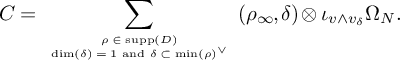 $$ \begin{align*}C = \sum_{ \tiny{\begin{array}{c} \rho\in\text{supp}(D) \\ \dim(\delta)=1 \text{ and } \delta \subset \min(\rho)^\vee \end{array}}} (\rho_\infty,\delta)\otimes \iota_{v\wedge v_\delta}\Omega_N. \end{align*} $$
This concludes the proof.
We now investigate what happens when $\delta ^{[1]}S = 0$
, (i.e., if
$\delta ^{[1]}S = 0$
, (i.e., if $[D_{|X_{T,T^{\circ }}}] = 0$
). In this case, the term
$[D_{|X_{T,T^{\circ }}}] = 0$
). In this case, the term $E^{2}_{0,n}$
is equal to
$E^{2}_{0,n}$
is equal to $H_n(X_{T^\circ ,T}; \mathcal {F}^{\mathbb {F}_2}_0)$
, and thus generated by S. More generally, the term
$H_n(X_{T^\circ ,T}; \mathcal {F}^{\mathbb {F}_2}_0)$
, and thus generated by S. More generally, the term $E^{k}_{0,n}$
is equal to
$E^{k}_{0,n}$
is equal to $H_n(X_{T^\circ ,T}; \mathcal {F}^{\mathbb {F}_2}_0)$
as long as
$H_n(X_{T^\circ ,T}; \mathcal {F}^{\mathbb {F}_2}_0)$
as long as $\delta ^{[j]} S = 0$
for all
$\delta ^{[j]} S = 0$
for all $j < k$
. The next theorem proves the other direction in Theorem 5.2.
$j < k$
. The next theorem proves the other direction in Theorem 5.2.
Theorem 5.5. If $\delta ^{[1]} S = 0$
, then
$\delta ^{[1]} S = 0$
, then
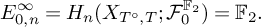 $$\begin{align*}E^{\infty}_{0,n} = H_n(X_{T^\circ,T}; \mathcal{F}^{\mathbb{F}_2}_0) = \mathbb{F}_2. \end{align*}$$
In particular, assuming (25), if $[D_{|X_{T,T^{\circ }}}] = 0$
, then the patchworking
$[D_{|X_{T,T^{\circ }}}] = 0$
, then the patchworking $X_{T^\circ ,T,\varepsilon }$
has two connected components.
$X_{T^\circ ,T,\varepsilon }$
has two connected components.
Proof. In the proof of Theorem 5.4, we constructed a lift of S as a chain ${\tilde S \in C_n(\mathcal {J}(T^\circ ,T);\mathcal {S}^{D})}$
. By taking its boundary, we obtained a (closed) chain
${\tilde S \in C_n(\mathcal {J}(T^\circ ,T);\mathcal {S}^{D})}$
. By taking its boundary, we obtained a (closed) chain $\partial \tilde S \in C_{n-1}(\mathcal {J}(T^\circ ,T);\mathcal {K}^{D}_1)$
, defining a class
$\partial \tilde S \in C_{n-1}(\mathcal {J}(T^\circ ,T);\mathcal {K}^{D}_1)$
, defining a class $[\partial \tilde S] \in H_{n-1}(\mathcal {J}(T^\circ ,T); \mathcal {K}^{D}_1)$
. The fact that
$[\partial \tilde S] \in H_{n-1}(\mathcal {J}(T^\circ ,T); \mathcal {K}^{D}_1)$
. The fact that $\delta ^{[1]}S = 0$
means that
$\delta ^{[1]}S = 0$
means that $[\partial \tilde S]$
maps to zero in
$[\partial \tilde S]$
maps to zero in $H_{n-1}(\mathcal {J}(T^\circ ,T); \mathcal {F}^{\mathbb {F}_2}_1)$
, in particular, it must be the image of a class
$H_{n-1}(\mathcal {J}(T^\circ ,T); \mathcal {F}^{\mathbb {F}_2}_1)$
, in particular, it must be the image of a class $\alpha _S \in H_{n-1}(\mathcal {J}(T^\circ ,T); \mathcal {K}^{D}_2)$
. By definition,
$\alpha _S \in H_{n-1}(\mathcal {J}(T^\circ ,T); \mathcal {K}^{D}_2)$
. By definition, $\delta ^{[2]} S$
is the image of
$\delta ^{[2]} S$
is the image of $\alpha _S$
in
$\alpha _S$
in $H_{n-1}(\mathcal {J}(T^\circ ,T); \mathcal {F}^{\mathbb {F}_2}_2)$
. We will prove that
$H_{n-1}(\mathcal {J}(T^\circ ,T); \mathcal {F}^{\mathbb {F}_2}_2)$
. We will prove that
 $$\begin{align*}[\partial \tilde S] = 0 \ \ \text{in} \ \ H_{n-1}(\mathcal{J}(T^\circ,T);\mathcal{K}^{D}_1). \end{align*}$$
This will imply $\delta ^{[k]} S = 0$
for all
$\delta ^{[k]} S = 0$
for all $k \geq 1$
and hence the statement of the theorem. We already proved that as a class in
$k \geq 1$
and hence the statement of the theorem. We already proved that as a class in $H_{n-1}(\mathcal {J}(T^\circ ,T);\mathcal {M}_1^{\mathbb {F}_2})$
,
$H_{n-1}(\mathcal {J}(T^\circ ,T);\mathcal {M}_1^{\mathbb {F}_2})$
, $\delta ^{[1]} S $
is represented by the cycle
$\delta ^{[1]} S $
is represented by the cycle
 $$\begin{align*}\gamma_1=\sum_{\rho\in\text{supp}(D)}\sum_{ \tiny{\begin{array}{c} (\delta,\rho)\in\mathcal{J}(T^\circ,T) \\ \dim(\delta)=1 \end{array}}} (\delta, \rho)\otimes (\tau_1 - \tau_2), \end{align*}$$
where $\tau _1$
and
$\tau _1$
and $\tau _2$
are the vertices of
$\tau _2$
are the vertices of $\delta $
. Since
$\delta $
. Since $\delta ^{[1]}S =0 $
, this cycle must be exact. So there exists a chain
$\delta ^{[1]}S =0 $
, this cycle must be exact. So there exists a chain
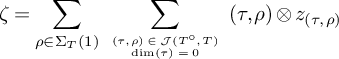 $$\begin{align*}\zeta = \sum_{\rho \in \Sigma_{T}(1)} \sum_{ \tiny{\begin{array}{c} (\tau,\rho)\in\mathcal{J}(T^\circ,T) \\ \dim(\tau)=0 \end{array}}} (\tau, \rho) \otimes z_{(\tau, \rho)}\end{align*}$$
in $C_{n}(\mathcal {J}(T^\circ ,T);\mathcal {M}_1^{\mathbb {F}_2})$
such that
$C_{n}(\mathcal {J}(T^\circ ,T);\mathcal {M}_1^{\mathbb {F}_2})$
such that
 $$\begin{align*}\partial \zeta = \gamma_1. \end{align*}$$
Notice that the coefficient $z_{(\tau , \rho )} \in \mathcal M_1(\tau , \rho ) = \rho ^{\perp }$
. We then have that the
$z_{(\tau , \rho )} \in \mathcal M_1(\tau , \rho ) = \rho ^{\perp }$
. We then have that the $z_{(\tau , \rho )}$
’s satisfy the following conditions
$z_{(\tau , \rho )}$
’s satisfy the following conditions
-
•
$z_{(\tau , \rho _1)}- z_{(\tau , \rho _2)} = 0\ \mod \tau $
, when
$\rho _1$
and
$\rho _2$
are edges of a two-dimensional simplex
$\lambda \in T$
; -
•
$z_{(\tau _1, \rho )}- z_{(\tau _2, \rho )} = \tau _1 - \tau _2$
, when
$\rho \in \operatorname {\mathrm {supp}} D$
and
$\tau _1, \tau _2$
are vertices of an edge
$\delta \in \partial T^{\circ }$
such that
$(\delta , \rho ) \in \mathcal {J}(T^\circ ,T)$
; -
•
$z_{(\tau _1, \rho )}- z_{(\tau _2, \rho )} = 0$
, when
$\rho \notin \operatorname {\mathrm {supp}} D$
and
$\tau _1, \tau _2$
are vertices of an edge
$\delta \in \partial T^{\circ }$
such that
$(\delta , \rho ) \in \mathcal {J}(T^\circ ,T)$
.


For any $\rho \in \Sigma _T(1)$
and some zero-dimensional
$\rho \in \Sigma _T(1)$
and some zero-dimensional $\tau \in T^{\circ }$
such that
$\tau \in T^{\circ }$
such that $(\tau , \rho ) \in \mathcal {J}(T^\circ ,T)$
, define the following vector:
$(\tau , \rho ) \in \mathcal {J}(T^\circ ,T)$
, define the following vector:
 $$\begin{align*}v_\rho = \begin{cases} z_{(\tau, \rho)} + \tau \quad \text{if} \ \rho \in \operatorname{\mathrm{supp}} D, \\ z_{(\tau, \rho)} \quad \text{if} \ \rho \notin \operatorname{\mathrm{supp}} D. \\ \end{cases} \end{align*}$$
The second and third bullet above imply that $v_\rho $
is independent of
$v_\rho $
is independent of $\tau $
; moreover, since
$\tau $
; moreover, since $z_{(\tau , \rho )} \in \rho ^{\perp }$
and
$z_{(\tau , \rho )} \in \rho ^{\perp }$
and $\tau \notin \rho ^{\perp }$
, we have that
$\tau \notin \rho ^{\perp }$
, we have that $v_\rho \in \mathcal E^D(\tau , \rho )$
. We use this vector to define a new lift of S in
$v_\rho \in \mathcal E^D(\tau , \rho )$
. We use this vector to define a new lift of S in $C_n(\mathcal {J}(T^\circ ,T);\mathcal {S}^{D})$
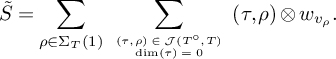 $$\begin{align*}\tilde S = \sum_{\rho \in \Sigma_T(1)}\sum_{ \tiny{\begin{array}{c} (\tau,\rho )\in\mathcal{J}(T^\circ,T) \\ \dim(\tau)=0 \end{array}}} (\tau,\rho)\otimes w_{v_\rho}. \end{align*}$$
Then the boundary of $\tilde S$
, as a chain in
$\tilde S$
, as a chain in $C_{n-1}(\mathcal {J}(T^\circ ,T);\mathcal {K}^{D}_1)$
is given by
$C_{n-1}(\mathcal {J}(T^\circ ,T);\mathcal {K}^{D}_1)$
is given by
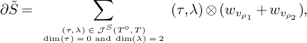 $$ \begin{align} \partial \tilde S =\sum_{ \tiny{\begin{array}{c} (\tau, \lambda)\in\mathcal{J}^S(T^\circ,T) \\ \dim(\tau)=0\text{ and } \dim(\lambda)=2 \end{array}}} (\tau,\lambda)\otimes (w_{v_{\rho_1}}+w_{v_{\rho_2}} ), \end{align} $$
where $\rho _1$
and
$\rho _1$
and $\rho _2$
are the two generators of the cone
$\rho _2$
are the two generators of the cone $C(\lambda )$
. Notice that there are no contributions from elements of type
$C(\lambda )$
. Notice that there are no contributions from elements of type $(\delta , \rho )$
, with
$(\delta , \rho )$
, with $\dim \delta = 1$
.
$\dim \delta = 1$
.
Suppose that $\lambda \in T$
is a two-dimensional simplex such that there are two distinct zero-dimensional elements
$\lambda \in T$
is a two-dimensional simplex such that there are two distinct zero-dimensional elements $\tau _1$
and
$\tau _1$
and $\tau _2$
such that
$\tau _2$
such that $(\tau _1, \lambda )$
and
$(\tau _1, \lambda )$
and $(\tau _2, \lambda )$
are both in
$(\tau _2, \lambda )$
are both in $\mathcal {J}(T^\circ ,T)$
. It follows from the definition of
$\mathcal {J}(T^\circ ,T)$
. It follows from the definition of $v_\rho $
that
$v_\rho $
that
 $$\begin{align*}v_{\rho_j} = z_{(\tau_k, \rho_j)} \mod \tau_k \quad \text{for} \ j,k \in \{1,2 \}, \end{align*}$$
and from the first bullet above, it follows that
 $$ \begin{align} v_{\rho_1} = v_{\rho_2} \mod \tau_k \quad \text{for} \ k \in \{1,2 \}. \end{align} $$
Since $T^{\circ }$
is primitive, we can assume that
$T^{\circ }$
is primitive, we can assume that $\tau _1$
and
$\tau _1$
and $\tau _2$
are linearly independent over
$\tau _2$
are linearly independent over $\mathbb {F}_2$
; therefore, we must have
$\mathbb {F}_2$
; therefore, we must have
 $$\begin{align*}v_{\rho_1} = v_{\rho_2}. \end{align*}$$
In particular, in (26), only those $\lambda $
’s for which there exists a unique zero-dimensional
$\lambda $
’s for which there exists a unique zero-dimensional $\tau $
such that
$\tau $
such that $(\tau , \lambda ) \in \mathcal {J}(T^\circ ,T)$
can contribute with a nonzero coefficient. Observe also that the latter property holds if and only if
$(\tau , \lambda ) \in \mathcal {J}(T^\circ ,T)$
can contribute with a nonzero coefficient. Observe also that the latter property holds if and only if $(\min \lambda )^\vee $
is zero-dimensional and
$(\min \lambda )^\vee $
is zero-dimensional and $\tau = (\min \lambda )^\vee $
is a vertex of
$\tau = (\min \lambda )^\vee $
is a vertex of $\Delta ^{\circ }$
. In this case,
$\Delta ^{\circ }$
. In this case, $\lambda _{\infty }$
is an edge in the interior of
$\lambda _{\infty }$
is an edge in the interior of $\tau ^\vee $
. Therefore, we may rewrite (26) in the following way:
$\tau ^\vee $
. Therefore, we may rewrite (26) in the following way:
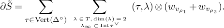 $$ \begin{align*} \partial \tilde S = \sum_{\tau \in \operatorname{Vert}(\Delta^\circ)} \sum_{ \tiny{\begin{array}{c} \lambda \in T, \dim(\lambda)=2 \\ \lambda_\infty \subset \operatorname{\mathrm{Int}}{\tau^\vee} \end{array}}} (\tau,\lambda)\otimes (w_{v_{\rho_1}}+w_{v_{\rho_2}} ). \end{align*} $$
The next goal is to prove that $\partial \tilde S$
is an exact chain in
$\partial \tilde S$
is an exact chain in $C_{n-1}(\mathcal {J}(T^\circ ,T);\mathcal {K}^{D}_1)$
. Indeed, define
$C_{n-1}(\mathcal {J}(T^\circ ,T);\mathcal {K}^{D}_1)$
. Indeed, define
 $$\begin{align*}\alpha = \sum_{\tau \in \operatorname{Vert}(\Delta^\circ)} \sum_{ \tiny{\begin{array}{c} \lambda \in T, \dim(\lambda)=2 \\ \lambda_\infty \subset \operatorname{\mathrm{Int}}{\tau^\vee} \end{array}}} (\tau,\lambda_{\infty})\otimes (w_{v_{\rho_1}}+w_{v_{\rho_2}} ). \end{align*}$$
Notice that $\alpha $
is supported on the infinite n-dimensional cells
$\alpha $
is supported on the infinite n-dimensional cells $F(\tau , \lambda _{\infty })$
which subdivide the cells
$F(\tau , \lambda _{\infty })$
which subdivide the cells $F(0, \lambda _{\infty }) \subset X_{T^\circ ,T}$
. We want to prove the following:
$F(0, \lambda _{\infty }) \subset X_{T^\circ ,T}$
. We want to prove the following:
-
•
$\alpha $
is a well-defined chain in
$C_{n}(\mathcal {J}(T^\circ ,T);\mathcal {K}^{D}_1)$
; -
•
$\partial \alpha = \partial \tilde S$
.


The first bullet amounts to proving that $v_{\rho _1}$
and
$v_{\rho _1}$
and $v_{\rho _2}$
are both in
$v_{\rho _2}$
are both in $\mathcal E^D(\tau , \lambda _{\infty })$
, so that the coefficients of
$\mathcal E^D(\tau , \lambda _{\infty })$
, so that the coefficients of $\alpha $
are in
$\alpha $
are in $\mathcal K^D_1$
. Recall that (27) holds (with
$\mathcal K^D_1$
. Recall that (27) holds (with $\tau = \tau _k$
), so either
$\tau = \tau _k$
), so either $v_{\rho _1}= v_{\rho _2}$
, in which case the coefficient of
$v_{\rho _1}= v_{\rho _2}$
, in which case the coefficient of $(\tau , \lambda _\infty )$
is zero, or
$(\tau , \lambda _\infty )$
is zero, or $v_{\rho _1}= v_{\rho _2} + \tau $
. Assume the latter holds. Since
$v_{\rho _1}= v_{\rho _2} + \tau $
. Assume the latter holds. Since $\lambda _{\infty } \subset \tau ^\vee $
, we have
$\lambda _{\infty } \subset \tau ^\vee $
, we have $\tau \in \lambda _\infty ^\perp $
; hence, either both
$\tau \in \lambda _\infty ^\perp $
; hence, either both $v_{\rho _1}$
and
$v_{\rho _1}$
and $v_{\rho _2}$
are in
$v_{\rho _2}$
are in $\mathcal E^D(\tau , \lambda _{\infty })$
, or both are not. The cells
$\mathcal E^D(\tau , \lambda _{\infty })$
, or both are not. The cells $(\tau , \lambda _\infty )$
,
$(\tau , \lambda _\infty )$
, $(\tau , \rho _1)$
,
$(\tau , \rho _1)$
, $(\tau , \rho _2)$
are the three n-dimensional cells intersecting along the
$(\tau , \rho _2)$
are the three n-dimensional cells intersecting along the $(n-1)$
-dimensional cell
$(n-1)$
-dimensional cell $(\tau , \lambda )$
. We already know that
$(\tau , \lambda )$
. We already know that $v_{\rho _1} \in \mathcal E^D(\tau , \rho _1)$
; therefore, using the properties of a real phase structure, it is enough to prove that
$v_{\rho _1} \in \mathcal E^D(\tau , \rho _1)$
; therefore, using the properties of a real phase structure, it is enough to prove that $v_{\rho _1} \notin \mathcal E^D(\tau , \rho _2)$
to conclude that
$v_{\rho _1} \notin \mathcal E^D(\tau , \rho _2)$
to conclude that $v_{\rho _1} \in \mathcal E^D(\tau , \lambda _{\infty })$
, and hence also
$v_{\rho _1} \in \mathcal E^D(\tau , \lambda _{\infty })$
, and hence also $v_{\rho _2}$
. We know that
$v_{\rho _2}$
. We know that $v_{\rho _2} \in \mathcal E^D(\tau , \rho _2)$
and that
$v_{\rho _2} \in \mathcal E^D(\tau , \rho _2)$
and that $\tau \notin \rho _2^\perp $
; hence, we must have that
$\tau \notin \rho _2^\perp $
; hence, we must have that $v_{\rho _1}= v_{\rho _2} + \tau $
cannot be in
$v_{\rho _1}= v_{\rho _2} + \tau $
cannot be in $\mathcal E^D(\tau , \rho _2)$
. This proves the first of the two bullets.
$\mathcal E^D(\tau , \rho _2)$
. This proves the first of the two bullets.
Let us now compute $\partial \alpha $
. We have
$\partial \alpha $
. We have
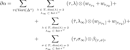 $$\begin{align*}\begin{aligned} \partial \alpha = \sum_{\tau \in \operatorname{Vert}(\Delta^\circ)} & \sum_{ \tiny{\begin{array}{c} \lambda \in T, \dim(\lambda)=2 \\ \lambda_\infty \subset \operatorname{\mathrm{Int}}{\tau^\vee} \end{array}}} (\tau,\lambda )\otimes (w_{v_{\rho_1}}+w_{v_{\rho_2}} ) + \\ \ & + \sum_{ \tiny{\begin{array}{c} \lambda \in T, \dim(\lambda)=2 \\ \lambda_\infty \subset \operatorname{\mathrm{Int}}{\tau^\vee} \end{array}}} (\hat \tau,\lambda_{\infty})\otimes (w_{[v_{\rho_1}]}+w_{[v_{\rho_2}]} ) + \\ \ & + \sum_{ \tiny{\begin{array}{c} \sigma \in T, \dim(\sigma)=3 \\ \sigma_\infty \subset \operatorname{\mathrm{Int}} \tau^\vee \end{array}}} (\tau,\sigma_{\infty})\otimes \beta_{(\tau, \sigma)}, \end{aligned} \end{align*}$$
where $[v_{\rho _j}]$
is the image of
$[v_{\rho _j}]$
is the image of $v_{\rho _j}$
under the projection
$v_{\rho _j}$
under the projection $\lambda _{\infty }^{\perp } \rightarrow \frac {\lambda _{\infty }^{\perp }}{\langle \tau \rangle }$
. The coefficient
$\lambda _{\infty }^{\perp } \rightarrow \frac {\lambda _{\infty }^{\perp }}{\langle \tau \rangle }$
. The coefficient $\beta _{(\tau , \sigma )}$
in the above formula is defined as follows. The three-dimensional simplex
$\beta _{(\tau , \sigma )}$
in the above formula is defined as follows. The three-dimensional simplex $\sigma $
has three boundary facets
$\sigma $
has three boundary facets $\lambda _1, \lambda _2$
and
$\lambda _1, \lambda _2$
and $\lambda _3$
containing the origin; therefore,
$\lambda _3$
containing the origin; therefore,
 $$\begin{align*}\beta_{(\tau, \sigma)} = \alpha_{(\tau,\lambda_{1, \infty})} + \alpha_{(\tau,\lambda_{2, \infty})} + \alpha_{(\tau,\lambda_{3, \infty})}, \end{align*}$$
where $\alpha _{(\tau ,\lambda _{j, \infty })}$
denotes the coefficient of
$\alpha _{(\tau ,\lambda _{j, \infty })}$
denotes the coefficient of $\alpha $
relative to the element
$\alpha $
relative to the element $(\tau , \lambda _{j, \infty })$
.
$(\tau , \lambda _{j, \infty })$
.
Since $v_{\rho _1} = v_{\rho _2} \mod \tau $
, we have that
$v_{\rho _1} = v_{\rho _2} \mod \tau $
, we have that
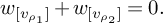 $$\begin{align*}w_{[v_{\rho_1}]}+w_{[v_{\rho_2}]} = 0. \end{align*}$$
Let us now prove that $ \beta _{(\tau , \sigma )} = 0$
. Label the edges and vertices of
$ \beta _{(\tau , \sigma )} = 0$
. Label the edges and vertices of $\sigma _{\infty }$
as in Figure 6. If all three edges are in
$\sigma _{\infty }$
as in Figure 6. If all three edges are in $\operatorname {\mathrm {Int}} \tau ^\vee $
, we have
$\operatorname {\mathrm {Int}} \tau ^\vee $
, we have
 $$\begin{align*}\beta_{(\tau, \sigma)} = w_{v_{\rho_2}}+w_{v_{\rho_3}} + w_{v_{\rho_3}}+w_{v_{\rho_1}} + w_{v_{\rho_1}}+w_{v_{\rho_2}} = 0. \end{align*}$$
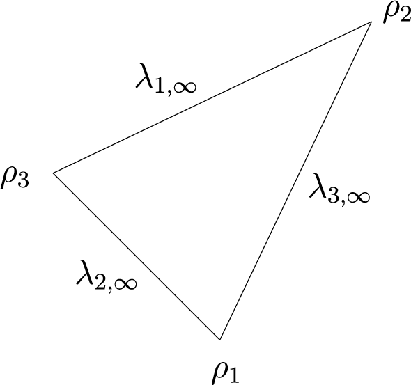
Figure 6 The boundary of $\lambda _{\infty }$
.
$\lambda _{\infty }$
.
If only one of the edges, say $\lambda _{1, \infty }$
, is in the boundary of
$\lambda _{1, \infty }$
, is in the boundary of $\tau ^{\vee }$
, it means that there exists another
$\tau ^{\vee }$
, it means that there exists another $\tau '$
such that
$\tau '$
such that $(\tau ', \lambda _1) \in \mathcal {J}(T^\circ ,T)$
, but then
$(\tau ', \lambda _1) \in \mathcal {J}(T^\circ ,T)$
, but then $\alpha _{(\tau , \lambda _{1,\infty })} =0$
and
$\alpha _{(\tau , \lambda _{1,\infty })} =0$
and
 $$\begin{align*}v_{\rho_2} = v_{\rho_3}. \end{align*}$$
Therefore,
 $$\begin{align*}\beta_{(\tau, \sigma)} = w_{v_{\rho_3}}+w_{v_{\rho_1}} + w_{v_{\rho_1}}+w_{v_{\rho_2}} = 0. \end{align*}$$
Similarly, $\beta _{(\tau , \sigma )} =0$
when two of the edges are in the boundary of
$\beta _{(\tau , \sigma )} =0$
when two of the edges are in the boundary of $\tau ^{\vee }$
. This proves that
$\tau ^{\vee }$
. This proves that $\partial \alpha = \partial \tilde S$
and concludes the proof of the theorem.
$\partial \alpha = \partial \tilde S$
and concludes the proof of the theorem.
Example 5.6. Let $D = \sum _{a_\rho } D_\rho $
be supported in the interior of the facets of
$D = \sum _{a_\rho } D_\rho $
be supported in the interior of the facets of $\Delta $
. Then
$\Delta $
. Then $D_{|X_{T,T^{\circ }}} = 0$
since divisors in the interior of maximal faces are mapped to vertices by the blowdown map
$D_{|X_{T,T^{\circ }}} = 0$
since divisors in the interior of maximal faces are mapped to vertices by the blowdown map $\operatorname {Bl}: \mathbb {T}\Sigma _{T} \rightarrow \mathbb {T}\Sigma _{\Delta ^{\circ }}$
. In particular,
$\operatorname {Bl}: \mathbb {T}\Sigma _{T} \rightarrow \mathbb {T}\Sigma _{\Delta ^{\circ }}$
. In particular, $X_{T^\circ , T, \epsilon }$
will have two connected components.
$X_{T^\circ , T, \epsilon }$
will have two connected components.
Example 5.7. Consider the divisors $D= D_7 + D_8$
and
$D= D_7 + D_8$
and $D= D_8$
as in Figure 5. In the first case,
$D= D_8$
as in Figure 5. In the first case, $D_{|X_{T,T^{\circ }}}$
is one point, and in the second,
$D_{|X_{T,T^{\circ }}}$
is one point, and in the second, $D_{|X_{T,T^{\circ }}} = 0$
(see Figure 7). The corresponding patchworkings are depicted in Figure 5, and they are respectivley connected and disconnected.
$D_{|X_{T,T^{\circ }}} = 0$
(see Figure 7). The corresponding patchworkings are depicted in Figure 5, and they are respectivley connected and disconnected.
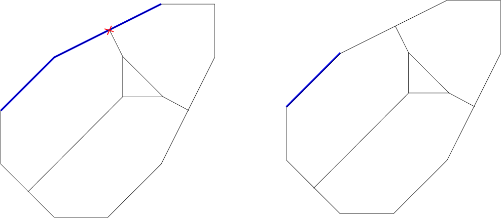
Figure 7 The intersection of $X_{T, T^\circ }$
with two different divisors.
$X_{T, T^\circ }$
with two different divisors.
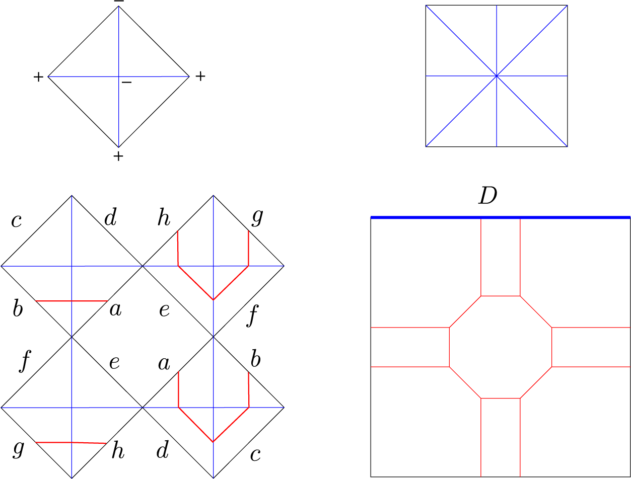
Figure 8 Two dual reflexive polygons. A divisor D in the mirror and the corresponding disconnected patchworking. The divisor intersects the mirror curve in two points (i.e., $D_{|X_{T,T^{\circ }}}=0$
).
$D_{|X_{T,T^{\circ }}}=0$
).
Example 5.8. Consider the two reflexive polytopes in Figure 8, where T is on the left. We have drawn an example of patchworking and the corresponding divisor. The divisor $D_{|X_{T,T^{\circ }}}$
consists of two points, and therefore, it is zero (
$D_{|X_{T,T^{\circ }}}$
consists of two points, and therefore, it is zero ( $\mod 2$
). Indeed,any patchworking in this example will be disconnected.
$\mod 2$
). Indeed,any patchworking in this example will be disconnected.
Acknowledgements
The authors wish to thank Erwan Brugallé, Mark Gross and Kris Shaw for useful discussions and also the referee for insightful suggestions. Diego Matessi was partially supported by the national research project ‘Moduli spaces and special varieties’ (PRIN 2022), and he is a member of the INDAM research group GNSAGA. Arthur Renaudineau acknowledges the support of the CDP C2EMPI, as well as the French State under the France-2030 programme, the University of Lille, the Initiative of Excellence of the University of Lille, the European Metropolis of Lille for their funding and support of the R-CDP-24-004-C2EMPI project, and also the ANR, project ANR-22-CE40-0014. Both authors wish to thank the FBK-CIRM and the Department of Mathematics at the University of Trento for their support and hospitality during the ‘Research in pairs program’.
Competing interest
The authors have no competing interest to declare.
Data availability statement
No data was produced or analyzed in this study.


 Open access