A novel adaptive sampling approach with batch selection for the automatic generation of surrogate models in geotechnical engineering

Abstract

Surrogate models have gained widespread popularity for their effectiveness in replacing computationally expensive numerical analyses, particularly in scenarios such as design optimization procedures, requiring hundreds or thousands of simulations. While one-shot sampling methods—where all samples are generated in a single stage without prior knowledge of the required sample size—are commonly adopted in the creation of surrogate models, these methods face significant limitations. Given that the characteristics of the underlying system are generally unknown prior to training, adopting one-shot sampling can lead to suboptimal model performance or unnecessary computational costs, especially in complex or high-dimensional problems. This paper addresses these challenges by proposing a novel, model-independent adaptive sampling approach with batch selection, termed Cross-Validation Batch Adaptive Sampling for High-Efficiency Surrogates (CV-BASHES). CV-BASHES is first validated using two analytical functions to explore its flexibility and accuracy under different configurations, confirming its robustness. Comparative studies on the same functions with two state-of-the-art methods, maximum projection (MaxPro) and scalable adaptive sampling (SAS), demonstrate the superior accuracy and robustness of CV-BASHES. Its applicability is further demonstrated through a geotechnical application, where CV-BASHES is used to develop a surrogate model to predict the horizontal deformation of a diaphragm wall supporting a deep excavation. Results show that CV-BASHES efficiently selects training samples, reducing the dataset size while maintaining high surrogate accuracy. By offering more efficient sampling strategies, CV-BASHES streamlines and enhances the process of creating machine learning models as surrogates for tackling complex problems in general engineering disciplines.

Impact Statement

Sampling strategies are essential in developing surrogate models for expensive numerical analyses. However, classic one-shot sampling methods often struggle with oversampling or undersampling issues, as accurately estimating the appropriate number of samples can be difficult. The novel adaptive sampling approach presented in this paper utilizes K-fold cross-validation (CV) error information to guide the selection of new samples, coupled with multiple distance criteria as hard constraints to ensure space-filling and non-collapsing properties. This method also supports batch selection, rendering it efficient for complex machine learning tasks when developing surrogate models.

1. Introduction

With the growing demand for more realistic and accurate computational analyses in various engineering fields, engineering simulations have become increasingly time-consuming. While this increased complexity improves the precision and reliability of the results, it also introduces significant challenges, particularly when there are time constraints in place or computational resources are limited, which often prevent their practical application.

To address these challenges, surrogate models have emerged as effective alternatives. These models act as mathematical approximations of the original numerical analyses, delivering results of comparable accuracy within a fraction of the time. By leveraging data from a limited number of simulations, surrogate models can provide rapid, accurate predictions without the need for full-scale computational analysis (Forrester et al., 2008). Their efficiency makes them particularly valuable in scenarios requiring a large number of simulations or real-time decision-making (Jones et al., 1998; Jones, 2001), e.g., civil engineering (Asher et al., 2015; Ninić et al., 2017; Qi and Fourie, 2018; Cao et al., 2020), aerospace engineering (Yondo et al., 2018), and chemical engineering (McBride and Sundmacher, 2019).

Among these disciplines, geotechnical engineering presents particularly demanding computational challenges. Numerical analyses used to simulate complex soil–structure interactions are often highly nonlinear and computationally intensive, mainly due to the advanced constitutive models required to simulate realistically the behavior of soils. Furthermore, the inherent uncertainty and spatial variability of soil properties mean that computationally expensive procedures such as sensitivity studies, probabilistic design, and real-time back-analysis are particularly relevant in geotechnics. Realistically, these procedures can only be implemented in geotechnical engineering practice using surrogate models, leading to their increased adoption in recent years.

Building upon these developments, surrogate models allow a range of engineering procedures, such as modeling and prediction, design optimization, and feasibility analysis (Bhosekar and Ierapetritou, 2018), to be conducted efficiently. Numerous studies have outlined methodologies for constructing robust surrogate models (Keane and Nair, 2005; Forrester et al., 2008; Hastie, 2009). However, defining the optimal number and characteristics of the samples required to create surrogate models remains a significant challenge in implementing this approach in practical engineering settings, since an insufficient number of samples can lead to inaccurate predictions, while an excessive number of samples may unnecessarily increase computational costs. This paper introduces Cross-Validation Batch Adaptive Sampling for High-Efficiency Surrogates (CV-BASHES), a novel adaptive sampling approach with batch selection to address the limitations of traditional single-point adaptive sampling methods which, as explained in the next section, are impractical for training complex machine learning models.

2. Sampling methods

Sampling strategies are generally classified into two broad categories: one-shot and sequential methods (Liu et al., 2018). Sequential methods can be further subdivided into space-filling sequential designs and adaptive sampling techniques. One-shot sampling entails generating the entire dataset in a single pass. A widely used strategy within this category is the Latin Hypercube Sampling (LHS) method (McKay et al., 1979), which ensures stratification in all subspace projections but does not guarantee that sample points are well spread across the exploration space. Other methods have been proposed to enhance the space-filling and non-collapsing properties of LHS, where non-collapsing means that the sample points maintain good projection distances. These include the Maximin criterion and the Minimax criterion (Johnson et al., 1990), which rely on optimization techniques to maximize/minimize the minimum/maximum distance between sample points. However, these approaches can be computationally intensive and may not always yield optimal sampling designs, particularly in high-dimensional spaces. Moreover, they suffer the inherent limitations of one-shot sampling mentioned above. These are addressed by space-filling sequential designs, which build upon the principles of one-shot sampling strategies while allowing for new sample points to be added iteratively over time. This feature, however, may come at the cost of deviating from the underlying principles of the original sampling strategy, which may be suboptimal, or by imposing constraints on the number of samples that can be selected in each iteration. Various sequential methods based on LHS are discussed in Santner et al. (2003), with additional approaches such as maximum projection (MaxPro; Joseph et al., 2020) and those proposed by Crombecq et al. (2011b). Even though sequential methods allow increasing the size of the dataset incrementally, they select points solely based on global exploration considerations (i.e., searching across the entire input space to identify regions of interest) and do not account for the surrogate response.

Unlike previously described sampling approaches, adaptive sampling methods consider both global exploration and local exploitation, the latter based on feedback from the surrogate response. Global exploration can be guided by distance minima (Li et al., 2010; Aute et al., 2013) or by utilizing the concepts of Voronoi cells through Monte Carlo approximation (Crombecq et al., 2011a; Xu et al., 2014). In contrast, local exploitation focuses on populating new samples in certain regions of the input space identified through a local refinement criterion that is computed based on the surrogate model. Figure 1 illustrates conceptually the underlying principles of each sampling strategy, with the adaptive sampling approach showing greater concentration of new samples (red dots) in areas where the gradients of the response surface are larger, rather than prioritizing a uniform distribution of samples as in the space-filling sequential design.

Figure 1. Comparison of different sampling strategies.

For adaptive sampling, local refinement criteria include prediction variance, CV error, disagreement between predictions with different surrogates, or local gradients (Liu et al., 2018; Fuhg et al., 2021). Among these, using the CV error offers two advantages over the other approaches. First, it is a model-independent adaptive sampling method, meaning it does not rely on internal properties of a specific surrogate model, such as the variance in Gaussian process (GP) models. Consequently, it can be applied across a wide range of surrogate types, including GP, support vector regression (SVR), and artificial neural networks (ANNs), in contrast to model-dependent criteria, such as prediction variance, which are restricted to a single model class. Second, it effectively assesses the generalizability of the surrogate model by evaluating its performance on unseen data, thereby providing critical error information for refinement. For this approach, there are two challenges that require consideration: estimating the surrogate error in unsampled regions, which may require supplementary methods, and mitigating clustering of newly sampled points, which can reduce the efficiency of the sampling process.

Li et al. (2010) proposed using degree of influence with an exponential function to assess the leave-one-out (LOO) CV error for unsampled areas, where LOO is a technique that sequentially designates each data point for validation while using the remaining data for training. The method assumes a mathematical relationship between the estimated error at unobserved points and that established at nearby sampled points, which is a key aspect of the point selection procedure. This approach is further complemented by a minimum distance criterion designed to mitigate clustering of sampled points. However, clustering cannot be prevented in areas of interest. Aute et al. (2013) enhanced the representation of the LOO error by a method known as space-filling cross-validation trade-off (SFCVT), where an additional surrogate model is employed to estimate the error in unsampled regions. Furthermore, they addressed issues of clustering by incorporating a space-filling Maximin distance criterion. Xu et al. (2014) also addressed the issue of clustering with a different approach that assumes points with the maximum error are located within the Voronoi cell exhibiting the largest LOO error. This cell is then represented by a set of sampled points generated using the Monte Carlo method. Subsequently, the selected point is the one furthest from the current Voronoi point within this generated set, thereby ensuring global exploration. More recently, Hu et al. (2024) advanced this line of research by introducing a hybrid sampling metric that combines LOO error, local nonlinearity, and the relative size of Voronoi cells. This integrated approach promotes more comprehensive global exploration by balancing local accuracy and broader coverage of the design space. However, none of the methods reviewed above natively support batch selection. Consequently, the sampling process is limited to single-point selection: the surrogate model is updated after each new sample is added into the training database, new CV errors are generated, and the process is repeated. While this approach is straightforward, it becomes inefficient for high-dimensional and complex problems where hundreds of samples are required to adequately explore the design space. In such cases, single-point selection leads to excessive sequential updates and prohibitive computational costs. Batch selection, by contrast, enables multiple samples to be incorporated simultaneously, improving scalability and so leading to a more practical approach for training computationally expensive models, such as ANNs and SVR, which are particularly useful for highly nonlinear numerical simulations that require more accurate surrogate models.

As opposed to adaptive sampling based on single-point selection, batch selection methods enable the selection of multiple points at once, leading to a more efficient adaptive sampling process. Braconnier et al. (2011) integrated LOO error estimation with a quad-tree data structure to implement batch selection. However, their results indicate that this approach suffers to keep the sampled points sufficiently distant from each other in subsequent iterations. Building on the SFCVT framework, Mohammadi et al. (2022) modified the LOO by incorporating expected squared LOO and employing expected improvement with correlation scaling factor via a repulsion function as the soft selection criterion to promote space exploration. In their approach, batch selection is achieved by updating the corresponding repulsion function after each new point is selected. Alternatively, expanding upon the work of Xu et al. (2014), Kaminsky et al. (2021) proposed using K-fold CV instead of LOO to reduce computational costs. Their approach ensures the feasibility of batch selection by updating the Voronoi cells after each new sample is added, with a greater emphasis on local exploitation.

This study specifically focuses on the development of a global surrogate model for modeling and prediction, a common application in the field of civil engineering, wherein a global surrogate refers to a model designed to approximate accurately predictions across the entire design space. A novel adaptive sampling approach is presented in this paper, which leverages K-fold CV error information, enhancing the SFCVT framework with the integration of two additional distance criteria. Furthermore, CV-BASHES also supports batch selection, thereby broadening its practical applicability. Following a detailed description of the proposed adaptive sampling methodology, a comprehensive comparison of the performance of CV-BASHES with that of SFCVT when applied to two analytical solutions is provided. The application of the proposed adaptive sampling approach in developing a surrogate model for deep urban excavations is demonstrated, accompanied by an in-depth analysis of the corresponding results. The study demonstrates that CV-BASHES offers a more efficient and adaptable solution, enabling the automatic generation of accurate surrogate models for geotechnical problems without the need to predefine the number of training samples. The novelty of this work lies in two key contributions: (i) the development of new criteria to enable batch selection and improve sample quality and (ii) the use of K-fold CV to enhance computational efficiency.

3. Proposed sampling approach

Building on the SFCVT (Aute et al., 2013) framework, the proposed CV-BASHES approach introduces three key mechanisms to ensure the reliability of the sampling process. First, it utilizes the error information derived from the surrogate model, which is constructed using an existing sampling database and evaluated through K-fold CV, in contrast to the LOO CV used in SFCVT. This error information is subsequently employed to train a GP model (Rasmussen, 2004) as an error predictor, hereafter referred to as the error surrogate, enabling the estimation of surrogate model errors in unsampled regions and effectively guiding the local exploitation process. Second, to facilitate global exploration, CV-BASHES combines the distance criterion from SFCVT, described in Section 2, with a novel projection distance constraint equation. Third, the concept of Voronoi cells is incorporated into the batch selection process in a novel way to ensure adequate spacing between selected points, thereby directing the adaptive method to prioritize space exploration.

3.1. Initial training database

The adaptive sampling approach needs an initial training database D to initiate the process. It is advisable to generate this database using a one-shot sampling method with good space-filling properties, such as an optimized LHS. Although the size of the initial database can influence the efficiency of the sampling process (excessively small databases produce less quality error information early in the process, while excessively large ones place unnecessary sample points in certain regions), the proposed method is designed to adapt and improve over successive iterations, allowing accurate surrogate generation provided the initial size is within a reasonable range. To ensure consistent feature scaling during surrogate training, the input variables are normalized prior to constructing the initial surrogate model by applying standard scaling methods such as MaxAbsScaler or MinMaxScaler (Pedregosa et al., 2011).

3.2. Error information generation

K-fold CV and LOO CV are used for estimating the generalization error of a model in machine learning. While both aim to assess the model’s performance, they differ significantly in terms of computational efficiency and their impact on the quality of the generated error associated with individual sample points.

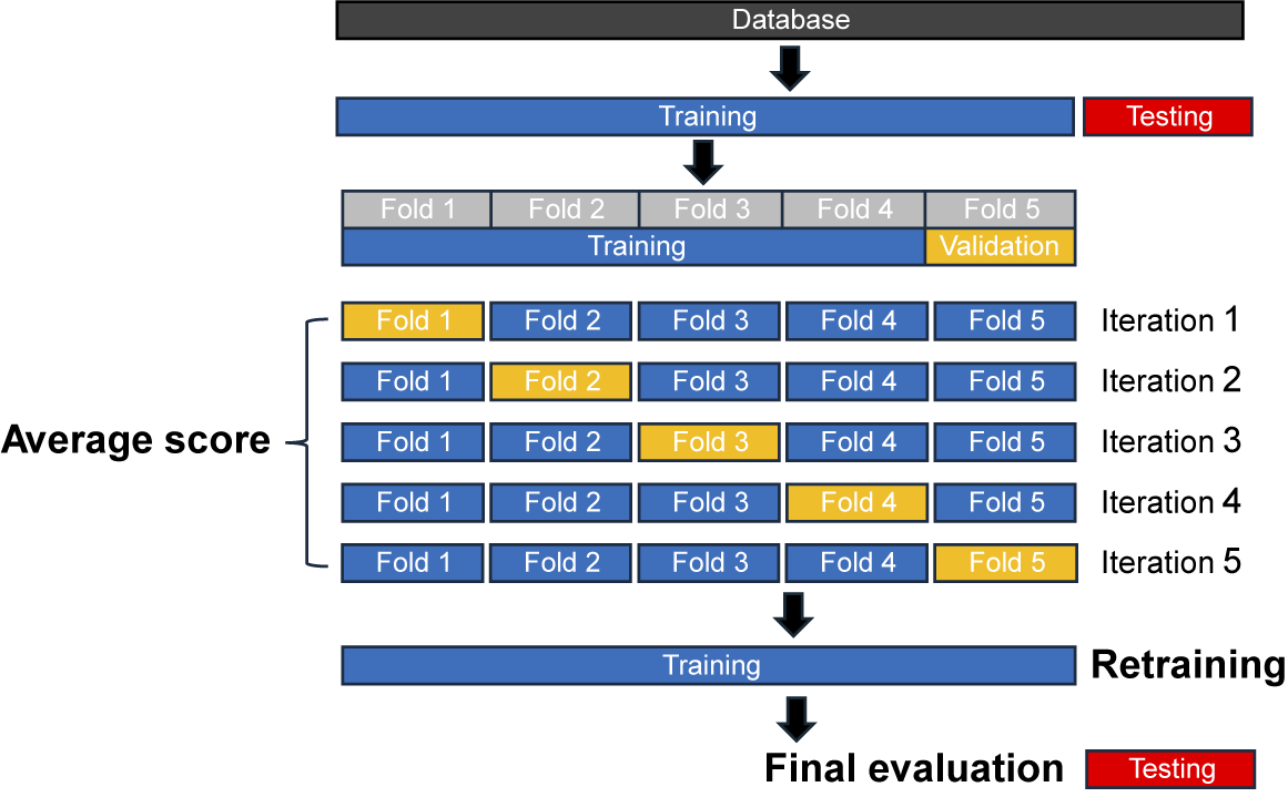
LOO is particularly suitable for scenarios where the dataset is small, as it involves n evaluations (where n is the number of samples), with each sample serving as the validation set exactly once, while the model is trained on the remaining (n−1) points. In contrast, K-fold CV requires only K evaluations of the model, as illustrated in Figure 2. Each fold is used as the validation set exactly once, and the model is trained on the remaining (K−1) folds. In the context of surrogate generation, where synthetic data are employed, K-fold CV tends to overestimate the error magnitude compared to LOO, particularly in the early stages of the sampling process when the training space is sparsely sampled and not well covered. This difference arises because K-fold CV trains on smaller subsets of the data, resulting in weaker models that may generalize less effectively than those trained on (n−1) points by LOO. Despite this, K-fold CV offers significantly improved computational efficiency, making it the preferred method in practice.

Figure 2. Five-fold cross-validation.

The coefficient of determination (R ²) is adopted as the metric to evaluate the surrogate error at the sample level, as each sample contains multiple output values that exhibit significant variation. Because R ² is dimensionless, it is particularly suitable to judge the error when the approximated output quantity (e.g., displacement, force) varies widely within a sample that shares similar input feature values. The error for a given sample x _i, consisting of n data points forming a curve, is computed as follows:

(1) $$ {e}_{\mathrm{K}-\mathrm{f}\mathrm{o}\mathrm{l}\mathrm{d}\hskip2pt \mathrm{C}\mathrm{V}}^{({\mathbf{x}}_i)}=1-\frac{\sum_{j=1}^n{(y({\mathbf{x}}_i^j)-\hat{y}({\mathbf{x}}_i^j))}^2}{\sum_{j=1}^n{(y({\mathbf{x}}_i^j)-\overline{y}({\mathbf{x}}_i))}^2} $$

where $ y,\hat{y} $ and $ \overline{y} $ are, respectively, the true output from the validation dataset for sample x _i, the surrogate’s prediction, and the mean of all true outputs for sample x _i. This equation is applied at the individual sample level, meaning R ² error is computed separately for each sample rather than across all validation samples at once. This approach is essential, as the error surrogate requires error information for each sample rather than a single overall score. However, when a sample contains only a single output data point, R ² is not applicable, as it requires a distribution of values to compute variance. In such scenarios, the normalized root mean squared error (RMSE) can serve as an effective alternative for assessing error magnitude. It is worth noting that the use of both K-fold CV and the R ² error metric represents methodological innovations introduced in this study, replacing the error estimation approach employed in the original SFCVT framework.

3.3. Error surrogate generation

There are several potential choices for the underlying model of the error surrogate, but it is crucial to balance performance and computational cost. In this approach, GPs are selected because, for the relatively small and noise-free datasets considered in this study, they provide smooth interpolations that closely reproduce the training database. The GP can be formulated as:

(2) $$ f\sim gp\hskip2pt (m(\mathbf{x}),k(\mathbf{x},{\mathbf{x}}^{\mathrm{\prime}})) $$

where $ m(\mathbf{x}) $ represents the mean function, typically assumed to be zero, and k denotes the covariance function. In this approach, the covariance function is specified by the radial basis function (RBF), given by:

(3) $$ k(\mathbf{x},{\mathbf{x}}^{\mathrm{\prime}})={\sigma}^2\mathrm{exp}\left(-\frac{{\Vert \mathbf{x}-{\mathbf{x}}^{\mathrm{\prime}}\Vert}^2}{2{l}^2}\right) $$

where σ ² is the signal variance and l is the length scale. The GP is used in conjunction with ten-fold CV and Grid Search (Géron, 2022) to determine the optimal combination of σ ² and l before establishing the final error surrogate.

3.4. Distance criteria

As outlined in Section 2, distance criteria must be enforced as hard constraints to prevent clustering of adapted sample points. The first criterion is based on the Maximin distance criterion S (Aute et al., 2013), defined as the Euclidean distance in the scaled space. This criterion ensures that new sample points remain sufficiently distant from existing ones. Initially, when the dataset contains fewer samples, the value of S tends to be relatively large. As a result, the selection of new samples is primarily governed by the distance criterion, leading to good space-filling properties. However, as sampling progresses, the value of S decreases, allowing for greater flexibility in local exploitation. For each point x _i in the database D, the minimum distance S(x _i) from this point to all the others is calculated as:

(4) $$ S({\mathbf{x}}_i)=\underset{i\ne j}{\min }(\Vert {\mathbf{x}}_i-{\mathbf{x}}_j\Vert )\hskip0.24em $$

Thus, S is calculated as half of the maximum value among all the minimum distances S(x _i):

(5) $$ S=0.5\times \max (S({\mathbf{x}}_i)) $$

The second criterion, which is used in conjunction with the first one, ensures diversity in newly selected sample points by considering input feature variation. Due to the isotropic nature of RBF kernel predictions, potential sample points may have similar predicted error magnitude, making selection ambiguous. While the RBF kernel length scale can be adjusted for each dimension, the overall error surrogate prediction distribution remains elliptical, limiting the ability to distinguish between equally viable candidates. To address this, a novel projection distance criterion is introduced to prioritize samples that differ more across input features. This criterion, S_pro, is derived from the LHS principle and is set as half the width of an LHS cell. It ensures that new samples are well spread across the feature space. The value of S_pro is calculated based on the total number of samples after incorporating newly added samples from the current iteration:

(6) $$ {S}_{pro}=0.5\times \frac{1}{\mathrm{num}\left(\mathrm{current}\ \mathrm{samples}\right)+\mathrm{num}\left(\mathrm{adapted}\hskip0.42em \mathrm{new}\hskip0.42em \mathrm{samples}\right)} $$

Voronoi cells (Voronoi, 1908) serve as the final criterion to ensure that the selected samples are sufficiently spaced apart during batch selection. These cells partition the space into regions based on the proximity to the nearest points, such that each point is associated with a specific cell, where any location within the cell is closer to its defining point (i.e., current sample point) than to any other cell point in the design space. Although computing the exact boundaries of Voronoi cells is computationally demanding, particularly in high-dimensional spaces, the proposed approach does not require explicit simulation of these boundaries. Instead, the Euclidean distance between a newly adapted point and the defining sample point of a cell is computed to determine which Voronoi cell contains the new point. Once identified, the corresponding cell is excluded from further selection within that sampling iteration. This process is introduced for the first time to enable batch selection and is discussed in detail in the following section.

3.5. Optimization strategy for batch selection

In most cases, batch selection in adaptive sampling effectively reduces computational costs by enabling simultaneous sampling in multiple regions. This shifts the optimization task from identifying a single global extremum to locating multiple local maxima or minima. While this challenge could potentially be addressed by conducting multiple trials of global optimization algorithms, each trial requires updating the penalty function. Moreover, their global search struggles to accurately identify the boundaries of these infeasible regions, which complicates the exploration of the entire feasible space and makes them impractical for real-world applications.

To address this, a novel methodology is introduced by adopting multiple steepest-ascent hill-climbing (Michalewicz, 2013) to solve the optimization problem. Hill-climbing is an iterative optimization algorithm that starts with an initial solution and moves to a better neighboring solution by making a small adjustment, referred to as the step size, based on an objective function. This process continues for a predetermined number of iterations or until no further improvements can be made, typically resulting in the identification of a local optimum.

To maximize efficiency and restrict the search to feasible regions, the hill-climbing algorithm is integrated with grid sampling. In this method, the starting points for hill-climbing are selected from a grid of points g, depicted as gray and blue dots in Figure 3. The gray dots, corresponding to infeasible regions defined by S and S_pro, are excluded from the optimization process. Only the blue dots g _i, located within the feasible regions (the non-shaded areas), are selected as valid starting points. The selected points satisfy the following mathematical conditions, where x _i is a point in the current database and d refers to the dimensionality of the problem:

(7) $$ \left\{\begin{array}{c}\Vert {\mathbf{g}}_i-{\mathbf{x}}_i\Vert >S,{\mathbf{x}}_i\in D,{\mathbf{g}}_i\in g\\ {}|{g}_{ik}-{x}_{ik}|>{S}_{pro},\mathrm{\forall}k=1,2,\dots, d,{\mathbf{x}}_i\in D,{\mathbf{g}}_i\in g\end{array}\right.\operatorname{} $$

Figure 3. Generation and pre-filtering of starting points for multiple hill-climbing.

Once the starting points are selected, each blue dot g _i serves as the initiation point for an independent hill-climbing search. A hypercube, centered around each point with side lengths equal to the grid resolution in each dimension, is designated as the search region. To ensure thorough exploration and promote diversity of the final solutions, a penalty function P(g _n) is introduced for neighboring points g _n, restricting the hill-climbing search within the boundary of this hypercube. The step size of the algorithm is set to 10% of the grid resolution, with a maximum of 10 iterations per realization, serving as the stopping criterion. Mathematically, this can be expressed as:

$$ P({\mathbf{g}}_n)=\left\{\begin{array}{c}0\hskip2.44em \mathrm{i}\mathrm{f}\hskip2pt |{g}_{nk}-{g}_{ik}|\le 5\times \mathrm{s}\mathrm{t}\mathrm{e}\mathrm{p}\ \mathrm{s}\mathrm{i}\mathrm{z}\mathrm{e},\mathrm{\forall}k=1,2,\dots, d\hskip2pt \\ {}\hskip-0.78em \mathrm{\infty}\hskip2.25em \mathrm{i}\mathrm{f}\hskip2pt |{g}_{nk}-{g}_{ik}|>5\times \mathrm{s}\mathrm{t}\mathrm{e}\mathrm{p}\ \mathrm{s}\mathrm{i}\mathrm{z}\mathrm{e},\mathrm{\forall}k=1,2,\dots, d\end{array}\right.\operatorname{} $$

(8) $$ {\mathbf{g}}_{new}=\left\{\begin{array}{c}{\mathbf{g}}_n\hskip0.839998em \mathrm{i}\mathrm{f}\ \mathrm{i}\mathrm{m}\mathrm{p}\mathrm{r}\mathrm{o}\mathrm{v}\mathrm{e}\mathrm{m}\mathrm{e}\mathrm{n}\mathrm{t}\ \mathrm{c}\mathrm{o}\mathrm{n}\mathrm{d}\mathrm{i}\mathrm{t}\mathrm{i}\mathrm{o}\mathrm{n}\ \mathrm{i}\mathrm{s}\hskip2pt \mathrm{m}\mathrm{e}\mathrm{t}\hskip0.24em \mathrm{a}\mathrm{n}\mathrm{d}\hskip0.24em P({\mathbf{g}}_n)=0\\ {}{\hskip-3em \mathbf{g}}_0\hskip1em \mathrm{i}\mathrm{f}\hskip2pt \mathrm{n}\mathrm{o}\hskip2pt \mathrm{v}\mathrm{a}\mathrm{l}\mathrm{i}\mathrm{d}\ \mathrm{n}\mathrm{e}\mathrm{i}\mathrm{g}\mathrm{h}\mathrm{b}\mathrm{o}\mathrm{u}\mathrm{r}\mathrm{s}\ \mathrm{o}\mathrm{r}\hskip2pt \mathrm{n}\mathrm{o}\hskip2pt \mathrm{i}\mathrm{m}\mathrm{p}\mathrm{r}\mathrm{o}\mathrm{v}\mathrm{e}\mathrm{m}\mathrm{e}\mathrm{n}\mathrm{t}\end{array}\right.\operatorname{} $$

where g _n is a potential new point from the neighbor and g ₀ is the current point (i.e., the current hill-climbing solution within this realization). During the hill-climbing search, the error surrogate is employed to evaluate the solutions generated within the assigned hypercube. The output values from the error surrogate are then used to assess and rank the solutions within the hypercube, guiding the search toward promising areas of the surrogate space. Therefore, each hypercube generates a single best solution based on the evaluation provided by the error surrogate.

The batch selection process for an adaptive sampling iteration is depicted in Figure 4. In the left panel (step 1), the infeasible solution space is represented by the gray-shaded area, representing the S and S_pro hard constraints. Upon evaluating the error surrogate (step 2), the unsampled point exhibiting maximum error (indicated by the orange dot) is selected as the first solution sample. The Voronoi cell containing the newly selected sample, highlighted by the red-shaded area, is subsequently excluded from the feasible solution space. Additionally, the newly adapted samples must satisfy the S and S_pro hard constraints relative to each other, as denoted by the blue-shaded rectangular and circular regions, which represent additional infeasible solution space. In the right panel (step 3), the process is repeated for an additional new sample point, with the updated constraints reflecting the inclusion of the second new sample. Mathematically, this can be expressed as:

$$ \hskip-14.8pc {\mathbf{x}}_n=\mathrm{arg}\underset{{\mathbf{x}}_o}{\max}\hat{y}({\mathbf{x}}_o) $$

$$ \hskip-11.5pc \mathrm{s}.\mathrm{t}.\hskip2.6em \Vert {\mathbf{x}}_o-{\mathbf{x}}_i\Vert >S,\mathrm{\forall}{\mathbf{x}}_i\in D $$

$$ \hskip-5.8pc \mathrm{s}.\mathrm{t}.\hskip2.6em |{x}_{ok}-{x}_{ik}|>{S}_{pro},\mathrm{\forall}k=1,2,\dots, d,\mathrm{\forall}{\mathbf{x}}_i\in D $$

$$ \hskip-5.8pc \mathrm{s}.\mathrm{t}.\hskip2.6em \Vert {\mathbf{x}}_o-{\mathbf{x}}_l\Vert >S,\mathrm{\forall}{\mathbf{x}}_l\in {\mathbf{x}}_n\hskip0.44em \mathrm{f}\mathrm{o}\mathrm{r}\hskip0.42em l=1,2,\dots, n $$

$$ \mathrm{s}.\mathrm{t}.\hskip2.6em |{x}_{ok}-{x}_{lk}|>{S}_{pro},\mathrm{\forall}k=1,2,\dots, d,\mathrm{\forall}{\mathbf{x}}_l\in {\mathbf{x}}_n\hskip0.24em \mathrm{f}\mathrm{o}\mathrm{r}\hskip0.42em l=1,2,\dots, n $$

(9) $$ \hskip-1.5pc \mathrm{s}.\mathrm{t}.\hskip2.36em {\mathbf{x}}_o\notin v({\mathbf{x}}_l),\mathrm{w}\mathrm{h}\mathrm{e}\mathrm{r}\mathrm{e}\hskip0.32em v({\mathbf{x}}_l)\hskip2pt \mathrm{i}\mathrm{s}\ \mathrm{t}\mathrm{h}\mathrm{e}\ \mathrm{V}\mathrm{o}\mathrm{r}\mathrm{o}\mathrm{n}\mathrm{o}\mathrm{i}\ \mathrm{c}\mathrm{e}\mathrm{l}\mathrm{l}\ \mathrm{c}\mathrm{o}\mathrm{n}\mathrm{t}\mathrm{a}\mathrm{i}\mathrm{n}\mathrm{s}\hskip2pt {\mathbf{x}}_l $$

Figure 4. Adaptive sampling process with constraint-based batch selection.

where x _l represents a point within the set of newly adapted solution samples x _n and x _o denotes a point in the unsampled area. As explained previously and repeated here for clarity, x _i is a point in the current database D and d refers to the dimensionality of the problem.

Following the generation of the solutions list by the hill-climbing search, a post-filtering process is applied. The solutions from hill-climbing search are ranked according to the magnitude of the associated error values returned by the error surrogate, with the top-ranked candidates being prioritized for selection. The hard constraints, including S, S_pro, and the exclusion of Voronoi cells, are then reapplied based on Equation 9 to ensure that all selected samples adhere to these feasibility criteria, relative to both the existing database and each other. In some cases, after applying the constraints, the number of valid solutions may be insufficient, as some solutions are excluded due to their proximity to others or because they violate the distance or projection criteria. In such instances, additional samples are randomly chosen from the top 10% of the ranked results from the hill-climbing process. This reapplication of constraints ensures that the selected solutions are both feasible and diverse.

3.6. Surrogate model update

Once the newly adapted samples are selected as described above, their response is calculated by evaluating the underlying computational model. Subsequently, the surrogate model is retrained with the expanded database. The training process includes tuning of the hyperparameters to identify an optimal configuration of the machine learning model. This approach facilitates further iterations if additional samples are required. As previously discussed, the proposed adaptive sampling method is model-independent, which allows adopting the most suitable model for any given application. This advantage has been exploited in Sections 4 and 5 where different models were employed as surrogates for some analytical functions and a finite element model of an urban excavation.

3.7. Stopping criteria

The proposed sampling approach considers two possible stopping criteria. In the first one, a target maximum error is specified such that when the global R ² of the newly trained surrogate model against the testing dataset is above that target, the surrogate model will be taken as final. A second criterion is made available for scenarios when the magnitude of the target error for the surrogate model cannot be established due to insufficient information about the system response. In the latter case, the process of surrogate generation will stop once the improvement in R ² is less than 0.01 over five consecutive iterations of the sampling procedure.

3.8. Step-by-step procedure of CV-BASHES

The flowchart for the proposed adaptive sampling approach, as illustrated in Figure 5, is outlined as follows:

Figure 5. Flowchart of the proposed adaptive sampling method.

• Step 1: Initialize with an initial database D generated using LHS;

• Step 2: Develop the initial surrogate model with database D;

• Step 3: Compute the K-fold CV error for all samples in D;

• Step 4: Employ Grid Search with ten-fold CV to develop the GP error surrogate;

• Step 5: Perform multiple hill-climbing optimizations with different starting points to identify local extrema;

• Step 6: Rank the optimization results and filtering by hard distance constraints;

• Step 7: Compute numerical response for the newly adapted samples;

• Step 8: Incorporate the adapted samples into the database; retrain the surrogate model;

• Step 9: Verify whether the stopping criterion is met. If not, return to step 3 and repeat the process.

4. Application to analytical functions

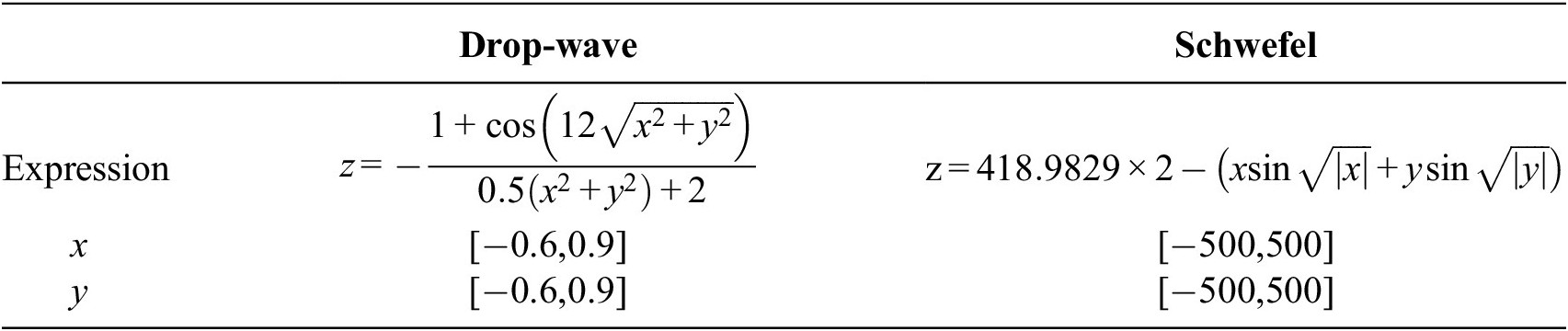
The performance of the proposed adaptive sampling approach was first assessed by generating surrogate models for two 3D analytical functions: a simple drop-wave function and the highly nonlinear Schwefel function. The expressions of both functions and the intervals considered for their variables are presented in Table 1, while the corresponding response surfaces are shown in Figure 6. In order to understand the effect of the various components of CV-BASHES, different configurations were adopted and their results were compared to those obtained with the SFCVT method as proposed in Aute et al. (2013).

Table 1. Details of the two analytical test cases

Figure 6. Response surface of drop-wave function (left) and Schwefel function (right).

4.1. Test setup and conditions

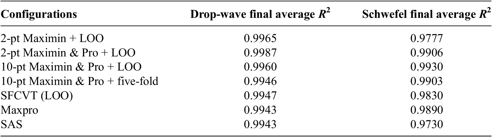
The tested configurations of the adaptive sampling method included: (a) two-point selection with the Maximin distance criterion and LOO validation, (b) two-point selection with the Maximin & Pro and LOO, (c) ten-point selection with Maximin & Pro and LOO, and (d) ten-point selection with Maximin & Pro and five-fold CV. All configurations employed batch selection and were constrained by Voronoi cells when choosing the solution samples. For SFCVT, the optimization problem was solved using genetic algorithms with appropriate parameters to ensure it consistently produced the best results. To assess the performance of CV-BASHES, two state-of-the-art sampling methods, MaxPro (Joseph et al., 2020) and scalable adaptive sampling (SAS) (Li et al., 2024), were included for comparison. Both methods were implemented using the parameter settings recommended in their respective original publications.

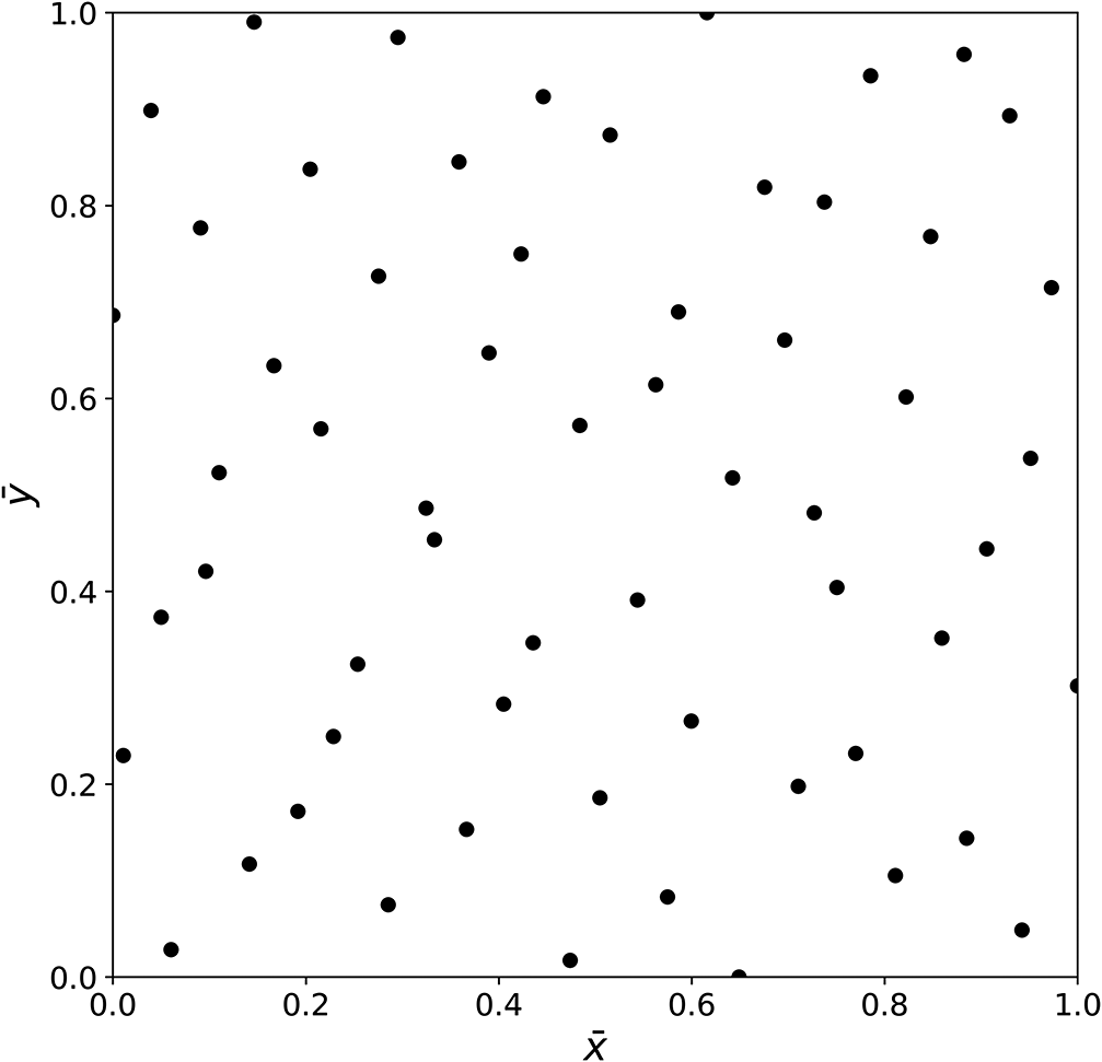
The initial databases for both functions consisted of 60 points generated using LHS with centered discrepancy optimization (Virtanen et al., 2020) and were equivalent when scaled to the range [0,1]; they are plotted in that scale in Figure 7.

Figure 7. Initial database for the two analytical test cases.

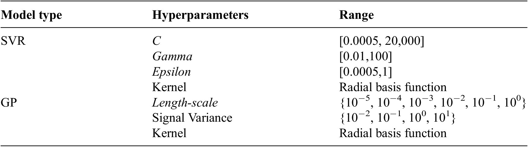
SVR (Smola and Schölkopf, 2004) was chosen as the intended surrogate model, with hyperparameter ranges specified in Table 2. Prior to training, the MaxAbsScaler (Pedregosa et al., 2011) was employed to scale the database. Hyperparameter tuning for the SVR was conducted using Random Search (Pedregosa et al., 2011), with 100 trials during each iteration of the adaptive sampling process. The RMSE was used to quantify the CV error for each sample point, which was then used to establish the error surrogate.

Table 2. Hyperparameter tuning intervals for SVR and GP

To model the error surrogate, GPs were tuned via Grid Search with the hyperparameter ranges outlined in Table 2. All simulations were conducted using scikit-learn (Pedregosa et al., 2011). To evaluate the accuracy of the SVR model, 10,000 random points were generated within the input space and evaluated using the analytical expressions in Table 1 to provide the test set. The sampling process continued until the R ² score on the test set exceeded 0.99 or the maximum number of samples was reached. The average testing R ² score was then computed across three independent runs for each case.

4.2. Results and discussion

The learning curve for both analytical examples are presented in Figure 8, with the intermediate (containing half the total number of samples of the final database) and the final database provided in Appendix A. The discussion is framed around five key perspectives: the effect of batch selection, the impact of the projection constraint, the use of either LOO or five-fold CV for error estimation, the comparison of CV-BASHES with SFCVT, MaxPro, and SAS, and the choice of batch size.

Figure 8. Learning curve of R² testing score for drop-wave function (left) and Schwefel function (right).

When employing two-point selection with only Maximin criterion (2-pt Maximin + LOO), the final surrogate’s accuracy was comparable to that of the SFCVT (LOO), establishing a baseline performance. However, incorporating the projection constraint into the two-point selection cases (2-pt Maximin & Pro + LOO) led to an improvement in performance. The projection constraint provides extra information through the more diverse spread of samples, thereby enhancing the surrogate model’s accuracy in both cases. Additionally, while the ten-point selection with Maximin & Pro and LOO (10-pt Maximin & Pro + LOO) showed a slightly better performance than the same configuration with five-fold CV error (10-pt Maximin & Pro + 5-fold), the difference was minimal. Given that five-fold CV is significantly more efficient than LOO—requiring far fewer surrogate model evaluations per iteration—it remains a practical choice for balancing accuracy and computational cost.

These findings demonstrate the effectiveness of CV-BASHES, which integrates additional projection and Voronoi cell constraints for batch selection. Compared to SFCVT, CV-BASHES excels in two key aspects: (a) it accelerates the adaptive sampling process, reducing the total running time, and (b) it produces a more accurate surrogate model with the same number of samples.

To contextualize further the performance of CV-BASHES, its results are compared to those of MaxPro and SAS. In the drop-wave example, all three methods, including SFCVT, achieved comparable results; however, CV-BASHES demonstrated superior performance when using two-point selection. For the more complex Schwefel function, SAS exhibited the poorest performance, while CV-BASHES slightly outperformed MaxPro. This outcome can be better understood by considering the fundamental differences between the methods. MaxPro is a purely global exploration technique, and its performance is independent of the number of samples in the initial database, whereas CV-BASHES adaptively selects new points based on both geometric diversity and surrogate error information. Consequently, in typical applications where the initial surrogate is reasonably accurate, CV-BASHES is expected to outperform MaxPro more substantially. In this example, the initial surrogate model was constructed with only 60 samples, resulting in a relatively low R ² of approximately 0.4. Even under these conditions, CV-BASHES achieved higher final accuracy than MaxPro, as shown in Table A1 and Figure 8. In practical scenarios, where the initial surrogate is generally more accurate, the advantage of CV-BASHES would be even more pronounced.

The choice of batch size depends on the response characteristics of the function being approximated. In the drop-wave example, the two-point selection resulted in the most accurate surrogate. This can be attributed to the surrogate being highly accurate from the outset of the process and so fewer regions requiring global exploration. For this kind of response shape, local exploitation is more effective. In contrast, the ten-point selection strategy emphasizes global exploration through Voronoi cells, making it more suitable for the Schwefel function: as shown in the figure, the ten-point selection configurations led to the most accurate surrogate. This final configuration proved particularly effective in the Schwefel function example, where it delivered comparable accuracy to that of LOO but with much better efficiency by combining a relatively large number of points per iteration with five-fold CV for error estimation. Similarly, in geotechnical engineering, where the target responses are typically highly nonlinear, selecting multiple points during the development of such models offers clear advantages. Based on these observations, it is recommended that batch sizes are chosen based on the complexity and nonlinearity of the response: smaller batches for simpler or well-behaved functions, and moderate to larger batches for complex, highly nonlinear functions.

5. ANN surrogate for an urban excavation

To illustrate the flexibility of CV-BASHES in terms of the machine learning model used and its application to a higher-dimensional problem, the proposed adaptive sampling method was used to establish an ANN-based surrogate model to predict the diaphragm wall horizontal movements resulting from the construction of a propped excavation within London Clay. This approach is particularly valuable in early stages of design, where in-situ data may be limited, enabling quick estimates of wall movements to support preliminary decision-making. Given that dozens of such excavations are conducted annually in London, with this number expected to rise, the trained surrogate model offers a cost-effective and reliable tool for preliminary design across a range of similar projects. In contrast to traditional numerical methods, the surrogate model offers immediate predictions that are free of convergence issues. It requires only the input of geometry parameters to rapidly produce results, thereby eliminating the need to rebuild or extensively modify the model when evaluating different design combinations during the preliminary design phase.

5.1. Description of the problem

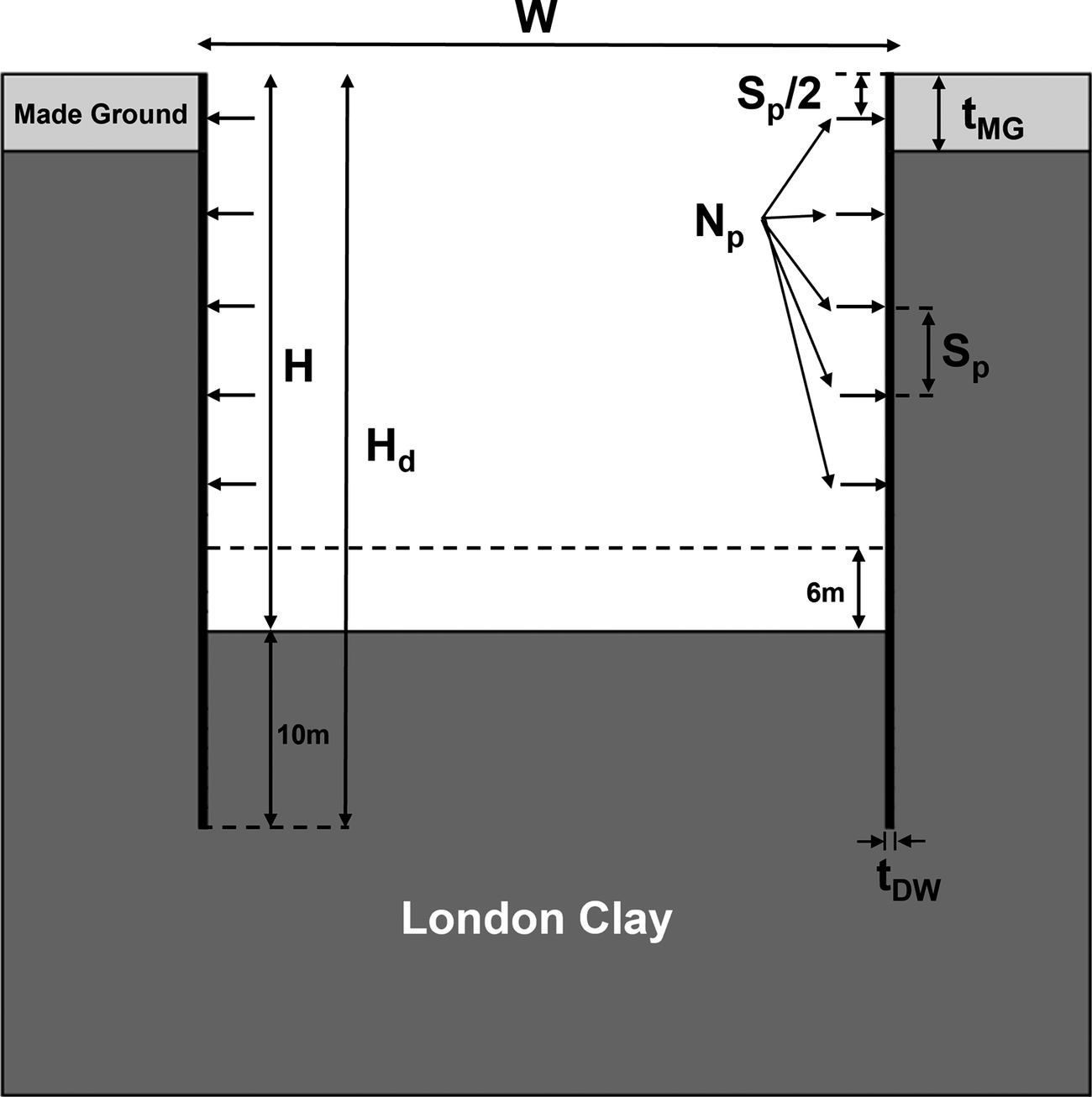
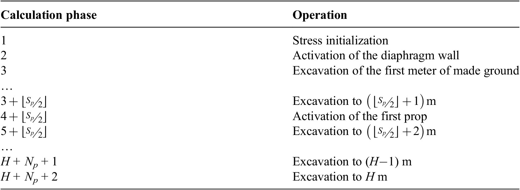
The problem was simulated numerically with plane strain analyses using the finite element software PLAXIS 2D 2024.01 (Bentley Systems, 2024), with a detailed description of the analysis setup being provided in Section 5.2. As shown in Figure 9, a simple stratigraphy consisting of a made ground layer overlying London Clay was considered. The excavation problem was defined parametrically allowing geometric variations in excavation width W, excavation depth H, prop spacing S_p, made ground layer thickness t_MG, and diaphragm wall thickness t_DW. It was assumed that the top prop was positioned S_p/2 below the ground level, while the bottom prop was placed at least 6 m above the excavation base. Moreover, the number of props N_P was calculated based on the depth of the excavation and the spacing between props using the following expression, which was rounded down to the nearest integer:

(10) $$ {N}_p=1+\lfloor \frac{H-\frac{S_p}{2}-6}{S_p}\rfloor $$

Figure 9. Parametric definition of the excavation problem.

Figure 10. Coefficient of earth pressure at rest (K₀) profile below the top of London Clay.

Drawing from several case histories of deep excavations in London (Wood and Perrin, 1984; Zdravkovic et al., 2011; Yeow et al., 2014; Chambers et al., 2016), the diaphragm wall was assumed to be embedded 10 m below the excavation depth H. The analysis sequence is detailed in Table 3. The excavation was assumed to progress in 1-m increments per calculation step. Furthermore, the props were activated in an additional step once the bottom of the excavation was below the corresponding prop level.

Table 3. Outline of the parameterized excavation sequence

5.2. Details of the analysis

Since the problem is symmetric around the center of the excavation, only half the domain was included in the analysis. The right far field boundary was located at a distance of 3H or 2.5 W from the plane of symmetry, whichever was larger, in order to prevent any boundary effects. Similarly, the bottom boundary was set such that the total depth of the model was twice the total height of the diaphragm wall H_d (see Figure 9). The soil domain was discretized using 15-noded triangular elements, with three refinement zones around the diaphragm wall where the largest stress gradients were expected. These zones were defined with widths of 0.3 m, 1 m, and 2 m and lengths of (H_d + 0.15) m, (H_d + 0.5) m, and (H_d + 1) m, respectively. The resulting mesh configurations varied in number of elements, ranging from 2542 elements for the case corresponding to W = 30 m and H = 10 m to 7640 elements for the largest structure, characterized by W = 80 m and H = 50 m.

An initial hydrostatic pore water pressure profile was adopted in the analyses, with the water table positioned at the top of the London Clay (i.e., at a depth of t_MG). The made ground layer was considered to be dry while undrained conditions were assumed for London Clay during the excavation, given its low permeability and the fact that excavations take place over relatively short periods of time. The initial coefficient of earth pressure at rest K ₀ along the depth of the made ground layer was set to 0.5, while in the London Clay layer, K ₀ was assumed to be 1.5 for the upper 10 m, linearly decreasing to 1.0 over the subsequent 10 m, and equal to 1.0 for the remaining depth (Schroeder et al., 2004; see). Regarding the mechanical boundary conditions, the horizontal displacements were restrained along the two vertical boundaries while both vertical and horizontal displacements were restrained along the bottom of the model.

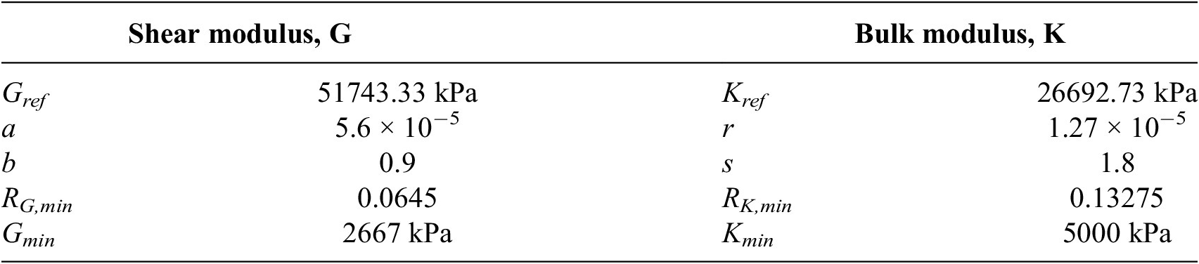
The mechanical behavior of made ground was simulated with linear elasticity and a non-associated perfectly plastic Mohr–Coulomb failure criterion. The elastic behavior was defined by a Young’s modulus E = 10 MPa and a Poisson’s ratio $ \nu $ = 0.2, while the strength was defined by a cohesion c′ = 0 kPa and an angle of shearing resistance ϕ′ = 30°, with a dilatancy angle ψ′ = 0^°. The unit weight of made ground was taken as 18 kN/m³. For London Clay, the material was simulated using IC MAGE M01 model (Taborda et al., 2023), implemented as a user-defined soil model in PLAXIS 2D, which incorporates the nonlinear elastic relationship for the tangent shear moduli G_tan and bulk moduli K_tan proposed by Taborda et al. (2016) along with a non-associated Mohr–Coulomb failure criterion. The stiffness parameters used in Gawecka et al. (2017) and Sailer et al. (2019) for the reproduction of case histories related to pile foundations and retaining walls, respectively, were adopted in this study and are listed in Table 4. The soil strength was defined by c’ = 5 kPa and ϕ′ = 25°, while the dilatancy angle was taken as ψ′ = 12.5^°. The unit weight of London Clay was adopted as 20 kN/m³.

Table 4. Stiffness properties adopted in IC MAGE M01 model for London Clay

The excavation support was typical of what is encountered in London Clay. The concrete diaphragm wall was assumed to be wished-in-place and simulated using beam elements. The wall was assumed to behave as a linear elastic material, characterized by a Young’s modulus E = 30 GPa and a Poisson’s ratio $ \nu $ = 0.3; a unit weight of 24 kN/m³ was adopted. Note that the bending and axial stiffness of the wall varied between analyses due to differences in wall thickness. The supporting props were assigned an axial stiffness of 50 MN/m/m, with an out-of-plane spacing equal to 5 m.

Lastly, the interaction between the soil and the wall was modeled using interface elements. These were extended to 1 m below the toe of the diaphragm wall such that the large stress concentration expected in that area could be dealt with during the numerical simulation. For the made ground layer, both interface strength and stiffness were calculated using a reduction factor of two-thirds relative to the surrounding soil, following the approach specified in Bentley Systems (2024). A similar approach was adopted for the London Clay layer, with the interface strength being determined using a reduction factor of two-thirds (c′_int = 3.33 kPa, ϕ′_int = 25°, ψ_int = 0^°). Given the nonlinear elastic model adopted for the stiffness of London Clay, a power-law was calibrated for the stiffness of the interface elements assuming a reduction factor of 1.0, yielding:

(11) $$ {E}_{oed}^{int}=531\;\mathrm{MPa}\times \left(\frac{\sigma_N^{\prime }}{100\;\mathrm{kPa}}\right) $$

5.3. Surrogate development

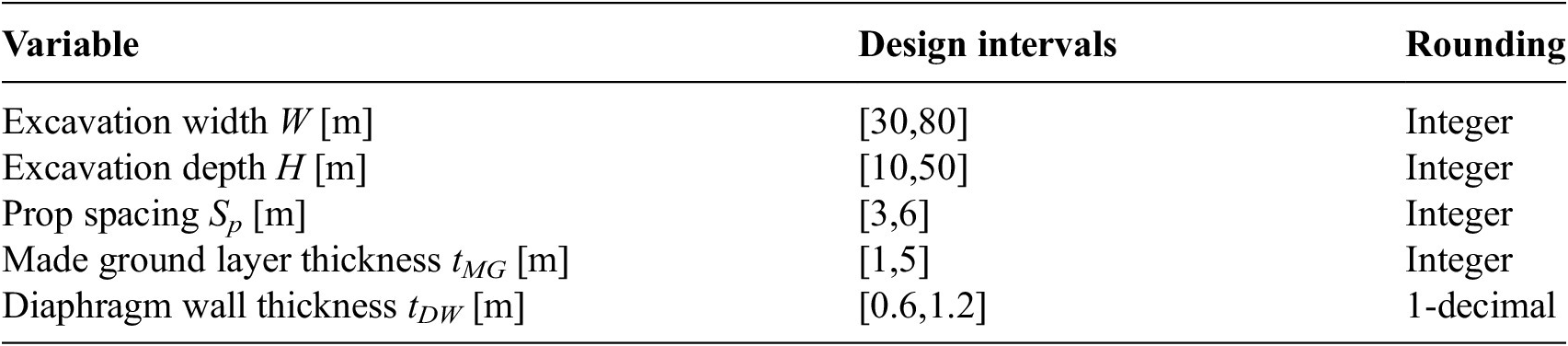
Utilizing the Python API in PLAXIS 2D (Bentley Systems, 2024), a script was developed to procedurally generate the geometry and construction sequence based on a defined set of parameters {W, H, S_p, t_MG, t_DW}. The script also automates the analysis and exports the diaphragm wall horizontal deformation for the final excavation phase. The initial database, comprising 20 distinct excavation geometries, was generated using LHS. Similarly, the testing database, which includes 100 additional cases, was also created using LHS to ensure comprehensive coverage of the design space. The design space for the surrogate is provided in Table 5.

Table 5. Design intervals for the ANN surrogate

The target wall deformation curve was approximated using 40 discrete, equally spaced points along the wall, with the depth denoted as y. Consequently, each sample in the database consisted of 40 points, with the parameters W, H, S_p, t_MG, t_DW, and N_p held constant across all points. However, the values of y and their corresponding deformation values varied for each point, representing the deformation profile along the wall. A visual representation of both the initial and testing databases is provided in Figure 11.

Figure 11. Visualization of the initial training database (left) and the testing database (right).

A feed-forward single-output ANN model, implemented in Keras (Chollet, 2015), was utilized to predict wall horizontal deformation using seven input features: W, H, S_p, t_MG, t_DW, N_p, and the normalized depth y/H_d, as illustrated in Figure 12. The Adam algorithm, an adaptive gradient descent method, was used as the optimizer during training of the ANN. The mean squared error (MSE) was adopted as the loss function. To mitigate overfitting, early stopping was employed with a patience value of 20 and a maximum of 150 epochs, meaning training was stopped if the validation score R ² did not improve for 20 consecutive iterations. A separate validation set, comprising 10% of the training data, was used for early stopping. This validation set was taken after initial split of the full dataset into training and validation sets and is distinct from the one used in the CV process described later. The HeUniform initialization (He et al., 2015) method was applied to the weights, and no activation function was used for the output layer.

Figure 12. Architecture of the single-output ANN.

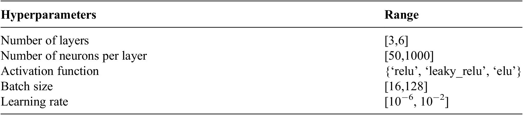
For the tuning of the ANN hyperparameters, the number of neurons per layer, number of layers, activation function, batch size, and learning rate were adjusted during each iteration of adaptive sampling, with intervals provided in Table 6. The optimal set of hyperparameters was selected through 100 trials of Random Search, based on the best validation score R ² from five-fold CV. The data were split to ensure that data points from the same excavation geometry were assigned to the same fold for training, validation, and early stopping.

Table 6. Hyperparameter tuning ranges for ANN optimization

The proposed adaptive sampling approach was implemented in an iterative manner, starting with an initial dataset comprising the 20 samples, each represented by 40 discrete points along the wall, for a total of 800 sample points, as depicted in Figure 11. In each iteration, the following operations were carried out: (i) hyperparameter tuning of the ANN was performed, with range specified in Table 6; (ii) the error surrogate was tuned as outlined in Section 3.3, with hyperparameter intervals specified in Table 2; (iii) the resolution for hill-climbing grid points was set to 0.05; (iv) the stopping criterion, based on the improvement in the R ² score for the 100 testing samples, was evaluated as outlined in Section 3.7. If the stopping criterion was not met, 10 new samples were selected according to the criteria outlined in Section 3.4 and 3.5. All developments of the ANN and the sampling process were executed on a system with a 12th Gen Intel(R) Core(TM) i7–12,700 CPU and 128GB of RAM, without GPU acceleration.

5.4. Results and discussion

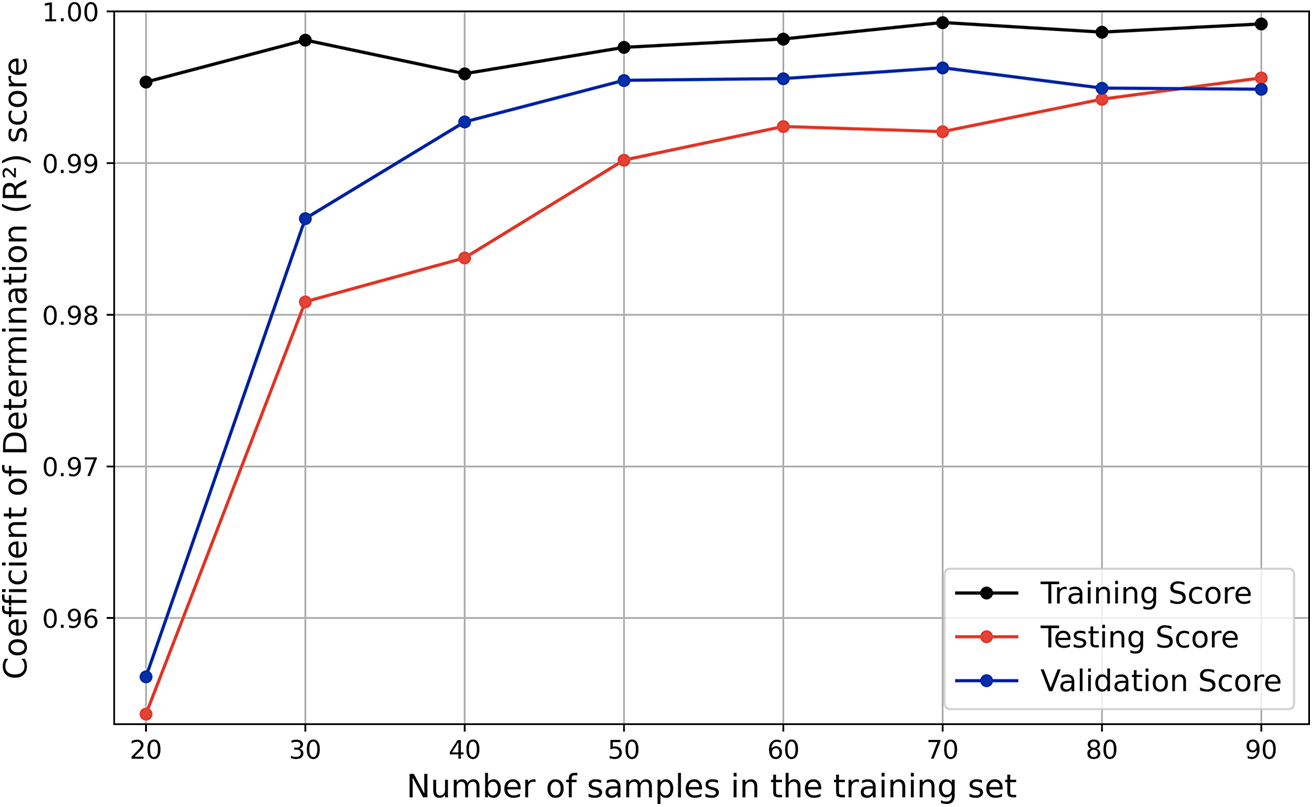
The final architecture of the ANN surrogate comprised four layers, each with 721 neurons and the exponential linear unit (ELU) activation function; a learning rate of 5.237 × 10⁻⁵; and a batch size of 22. Figure 13 presents the learning curve of the ANN surrogate, showcasing the model’s performance improvement across successive adaptive sampling iterations. The adaptive sampling procedure carried out seven iterations before the stopping criterion was satisfied, yielding a database of a total of 90 training samples. It can be observed that the performance of the ANN, in terms of validation and testing, improved rapidly for the first three iterations and more gradually thereafter. The results demonstrate good generalization of the ANN surrogate, achieving R ² scores, at the end of the sampling procedure, of 0.9949 on the validation set, 0.9956 on the testing set, and 0.9992 on the training set. The close alignment of the validation and testing scores is evidence of the robustness of the model.

Figure 13. Learning curve of the ANN surrogate with CV-BASHES.

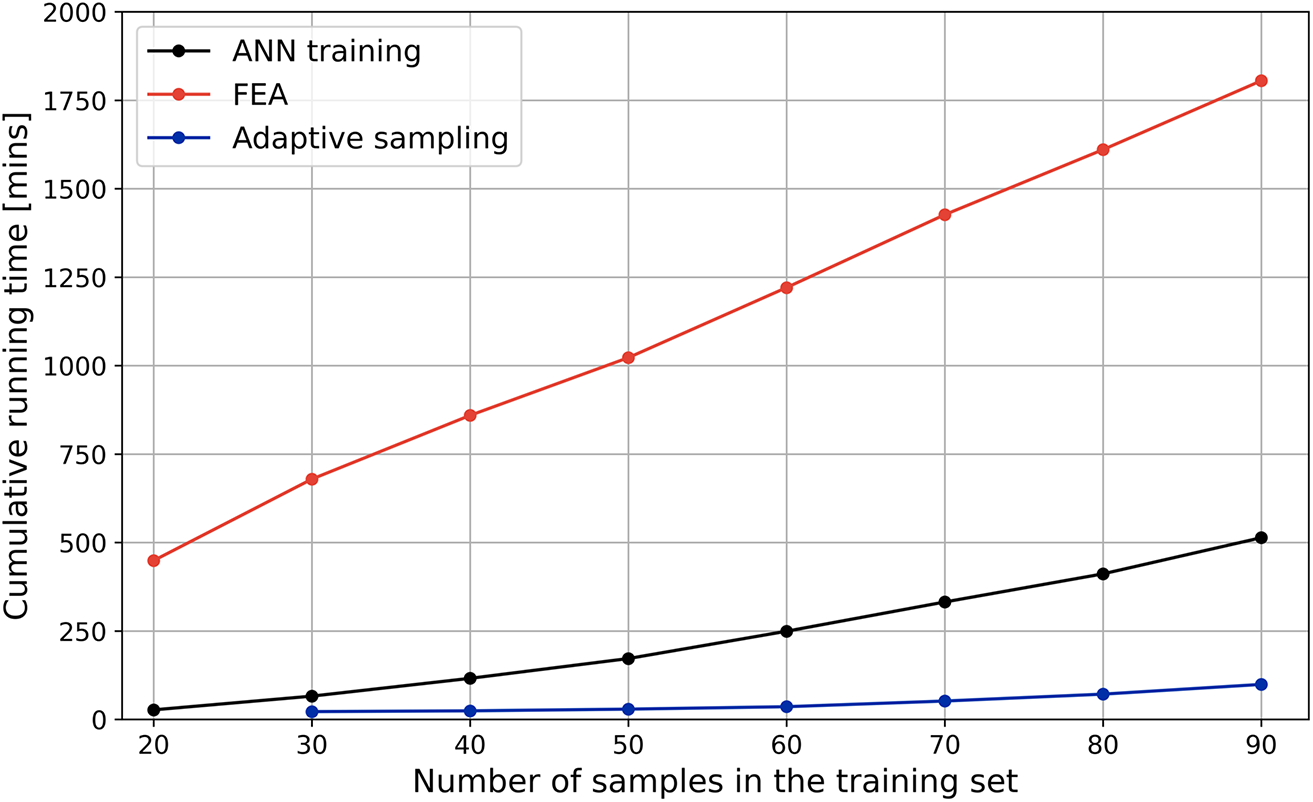
Figure 14 presents the total computational time required for the construction of the surrogate model with the adaptive sampling methodology. The breakdown of the cumulative computational effort indicates that the finite element analysis (FEA) accounts for the majority of the time, requiring approximately 30 h. In contrast, training the ANN surrogate—including retraining after each sampling iteration and 100 Random Search trials—takes significantly less time at 8 h. CV-BASHES—including error generation, fine-tuning the error surrogate, and running the optimization algorithm to identify solution candidates—requires just 1.5 h. Even though the FEA requires most of the computational effort, it is worth noting that, for the selected application, a single analysis was relatively fast to run (about 20 mins) and so, for more computationally demanding applications, the differences between the proportion of the time required by FEA and ANN training should be even larger. Given that the cost of generating the surrogate mostly comes from the FEA, for efficiency purposes, minimizing the number of analyses is clearly critical. The proposed sampling strategy effectively allows for the time spent running analyses to be reduced, without compromising the accuracy of the resulting surrogate model. Furthermore, it eliminates the need to decide beforehand, and without information about the system, on the number of analyses to be conducted.

Figure 14. Computational time for developing the ANN surrogate with CV-BASHES.

To examine further the performance of the surrogate model, Figure 15 depicts comparison plots for the training (a) and testing (b) datasets and the residual values between the surrogate and the numerical predictions, also for training (c) and testing (d). Both types of plots demonstrate that the surrogate is very accurate. The data points plot very closely to the “ideal fit” (1:1, red dashed) line in the comparison plots along the whole range of displacements; the residual of most points plot in a band of ±10 mm. This demonstrates the surrogate model’s strong predictive accuracy, including at higher displacement values, such as those exceeding approximately 220 mm in the testing dataset. Furthermore, the generalization ability of the surrogate is evaluated with two boxplots in Figure 16, where the distribution of the RMSE and R ² values for individual testing samples is illustrated. The annotated median values reveal that 50% of the testing samples achieve a RMSE below 2.124 mm and a R ² exceeding 0.995. Figure 17 shows the displacements along the depth of the wall as predicted by the surrogate and the numerical models for four specific geometries extracted from the testing database: that with the lowest R ² (a), that with the highest RMSE (c), which are the surrogate’s least accurate predictions for such metrics, and the samples corresponding to the 75th percentile of R ² (b) and RMSE (d) (i.e., 75% of the testing samples are more accurate). These plots demonstrate clearly that the surrogate is able to match the shape and magnitude of the wall movements even for less accurate samples. Moreover, CV-BASHES enabled such high accuracy to be achieved with an optimal number of samples, which were selected automatically, ultimately preventing the use of excessive computational resources and facilitating future streamlined creation of surrogates.

Figure 15. Comparison (a,b) and residual (c,d) plots of the final surrogate: training (a,c) and testing (b,d).

Figure 16. Boxplots of the final surrogate model on RMSE (left) and R² (right) score for testing data.

Figure 17. Analysis of the ANN’s worst (a,c) and 75th percentile (b,d) performance as judged by the R² (a,b) and RMSE (c,d) scores.

6. Conclusions

This study introduces CV-BASHES, a novel adaptive sampling approach for the automatic creation of global surrogate models. The proposed framework strategically prioritizes global exploration when the sample database is small, progressively shifting toward greater flexibility in local exploitation by relaxing distance criteria constraints as the sample database expands and surrogate model accuracy improves.

When compared to the SFCVT method, as well as two state-of-the-art sampling strategies, MaxPro and SAS, CV-BASHES outperforms them in terms of R ² testing score for two analytical examples, one of which is characterized by extreme nonlinearity, which makes it a suitable example to benchmark a technique intended to be applied to the highly nonlinear problems often encountered in geotechnical engineering. This example illustrates the method’s enhanced efficiency and ability to construct global accurate surrogate models.

A practical application, involving the automatic generation of an ANN surrogate for urban propped excavations, demonstrates that CV-BASHES can be paired with complex machine learning models and, most importantly, its effectiveness to yield accurate surrogate models for geotechnical problems. A detailed study of computation time shows that, while the newly introduced method is considerably more complex than others in the literature, its share of the required computational effort is negligible when compared to those of the FEA and the training of the machine learning models. Moreover, the results show large gains in accuracy during the first steps of the proposed adaptive sampling method, which fade as the number of samples increases. This allows the process of sampling to be stopped, saving computational resources that would otherwise be employed in the evaluation of new samples that would not translate into any additional benefits in terms of accuracy of the resulting surrogate.

Therefore, this work represents a significant advancement in surrogate generation in geotechnical engineering, eliminating the need to predetermine the optimal number of samples for the training database. This removes common challenges associated with sample size determination, allowing for a more dynamic and adaptive approach to surrogate model development, while guaranteeing high levels of accuracy. Although demonstrated through a geotechnical application, the CV-BASHES framework is general in formulation and applicable to other computationally intensive engineering problems requiring efficient surrogate modeling.