Evaluating CMIP6 models for near-surface air temperature projections over Antarctic ice shelves

Abstract

The meltwater-driven disintegration of the Larsen B ice shelf has raised concerns that other ice shelves may face similar vulnerabilities as global temperatures rise. Climate projections show increased ice shelf vulnerability to surface melt in the coming century, yet the ability of large-scale climate models to simulate temperatures over ice shelves—a key factor in these projections—has rarely been assessed. We address this gap by using ERA5 reanalysis data to evaluate 31 CMIP6 models’ performance in simulating near-surface air temperatures over 46 Antarctic ice shelves from 1979 to 2014. We find that CMIP6 models exhibit annual and summer warm biases over most ice shelves. There is also inter-model variability of up to 13°C between model temperatures over the Amery and Riiser-Larsen shelves for both annual and summer periods. Significant regional differences are present: shelves in the Amundsen Sea Embayment show cold biases, while those in the Weddell Sea show warm biases. While topography corrections can reduce some biases, we find notable seasonal differences, including biases with opposite signs between annual and summer means. Our results underscore the importance of careful model selection by shelf and region to improve the reliability of future climate projections and assessments of Antarctic ice shelf vulnerability.

1. Introduction

Ice shelves—floating platforms of ice that fringe the Antarctic Ice Sheet—play a key role in controlling the response of the Antarctic ice sheet to climate change. Ice shelves limit the mass discharged from grounded ice into the ocean through buttressing (e.g. Dupont and Alley, 2005; Gudmundsson, 2013; Pegler, 2018). Ice shelves gain mass via inflow across the grounding line, snow accumulation and accretion of marine ice at the bottom of the shelf, and lose mass through surface melt, basal melt and calving (Shepherd and others, 2012; Rignot and others, 2013; Mottram and others, 2021). Surface melt, although a small part of the total mass balance, has significantly impacted ice shelves in the Antarctic Peninsula; in some cases, surface melt is hypothesized to cause ice shelf collapse (e.g. Rott and others, 2002; Scambos and others, 2004; Kuipers Munneke and others, 2014). In this region, surface temperatures increased more rapidly than in the rest of Antarctica, resulting in the rapid meltwater-driven disintegration of Larsen A in 1995 and Larsen B in 2002 (Scambos and others, 2000, 2004; van den Broeke, 2005). The acceleration of tributary glaciers in the wake of collapse further demonstrated the buttressing effect of ice shelves on the discharge of grounded ice (e.g. Rott and others, 2002; Scambos and others, 2004).

The precise mechanisms leading to ice shelf collapse remain controversial, with hints that the final collapse may have been preconditioned by longer-term environmental forcing (e.g. Shepherd and others, 2003; Glasser and Scambos, 2008; Banwell and MacAyael, 2015; Rendfrey and others, 2025), but the speed of disintegration raises concerns that future warming will expose more ice shelves to longer and more severe melt seasons with the potential to destabilize them. Recognizing this vulnerability, the Ice Sheet Model Intercomparison Project (ISMIP6) developed an experiment in which ice shelves instantaneously collapse after a 10-consecutive-year period with melt above 775 mm w.e. yr ⁻¹ (Trusel and others, 2015; Nowicki and others, 2016, 2020; Seroussi and others, 2020). Trusel and others (2015) derived this threshold using near-surface air temperature data. The threshold is based on how well a subset of the models that participated in the Coupled Model Intercomparison Project Phase Five (CMIP5) could reproduce near-surface air temperatures from the European Centre for Medium-Range Weather Forecasts’ Interim reanalysis product (ERA-Interim) over Antarctic ice shelves (Trusel and others, 2015).

The newest CMIP6 models offer significant advancements over CMIP5 in climate modeling capabilities, including enhanced spatial resolution, improved cloud representation, and integrated socioeconomic pathways (Eyring and others, 2016).

Although the CMIP5 and CMIP6 models have been evaluated over grounded ice sheets, few studies have evaluated how the models perform over ice shelves. For example, Tewari and others (2022) evaluated the ability of CMIP6 models to reproduce near-surface air temperatures over the Antarctic ice sheet, but specifically excluded the floating ice shelves from their analysis. Nonetheless, Tewari and others (2022) identified a significant decadal warming trend over Antarctica from 2015 to 2099, ranging from 0.4°C to 0.8°C per decade. Li and others (2023) further analyzed biases in CMIP6 models by comparing simulated present-day (1981–2010) austral summer (December to February, DJF) near-surface air temperature and 400-m annual ocean potential temperature against observations over the Antarctic ice sheet, ice shelves, and the surrounding ocean. They observed substantial spatial heterogeneities, with some models showing a warm bias over the ice sheet and a cold bias over the ocean. Additionally, they found considerable inter-model variation, with two-meter air temperature biases over the ice shelves being as high as 8°C for some models. Although Li and others (2023) included ice shelves in their assessment, their focus was limited to austral summer biases and did not provide an in-depth model-level evaluation.

These studies underscore the presence of near-surface air temperature biases in CMIP6 models over the Antarctic region. However, accurately projecting surface melt and potential ice shelf collapse requires a more comprehensive evaluation of model performance over individual ice shelves, encompassing both temperature biases and interannual variability. We address this gap by determining which models, if any, can accurately reproduce the near-surface air temperature and magnitude of the interannual variability of the European Centre for Medium-Range Weather Forecasts’ fifth-generation reanalysis product (ERA5). We do this by examining the capability of the CMIP6 models to reproduce near-surface air temperatures through comparisons with ERA5 over 46 ice shelves from 1979 to 2014.

2. Data

2.1. ERA5

We base our analysis on the ERA5 reanalysis product (e.g. Laloyaux. and others, 2016). ERA5 is a comprehensive atmospheric reanalysis product that provides hourly estimates of atmospheric, land, and ocean climate variables from January 1940 to the present using a 4D-Var data assimilation algorithm (Laloyaux and others, 2016). Given the limited observations over ice shelves from the Antarctic Automatic Weather Station (AWS) Project, we use ERA5’s 2-m atmospheric temperature as a substitute. ERA5 represents the latest in reanalysis products, succeeding ERA-Interim, which produced the closest match for surface temperature in Antarctica among other available reanalysis products, given limited observational data (e.g. Bromwich and others, 2011; Behrangi and others, 2016; Tewari and others, 2022). A recent study by Zhu and others (2021) found that ERA5-modeled monthly surface temperatures over Antarctica show low monthly bias (−0.44°C to 1.19°C) and strong monthly correlation coefficients compared to 41 observational stations from 1979 to 2019.

Substituting reanalysis data for direct observations allows us to use a time-consistent, gridded dataset for comparison with CMIP6 model data. However, it also introduces the potential for error in our analysis, particularly over data-sparse regions. Importantly, while ground station observations are assimilated into ERA5, the scarcity of direct measurements over some ice shelves means that ERA5’s representation of near-surface air temperature may itself be uncertain in these areas. Therefore, our estimate of CMIP6 model biases based on ERA5 may have some error in data-sparse regions. For our study, we use monthly averaged temperatures for comparison with CMIP6 models.

2.2. CMIP6 models

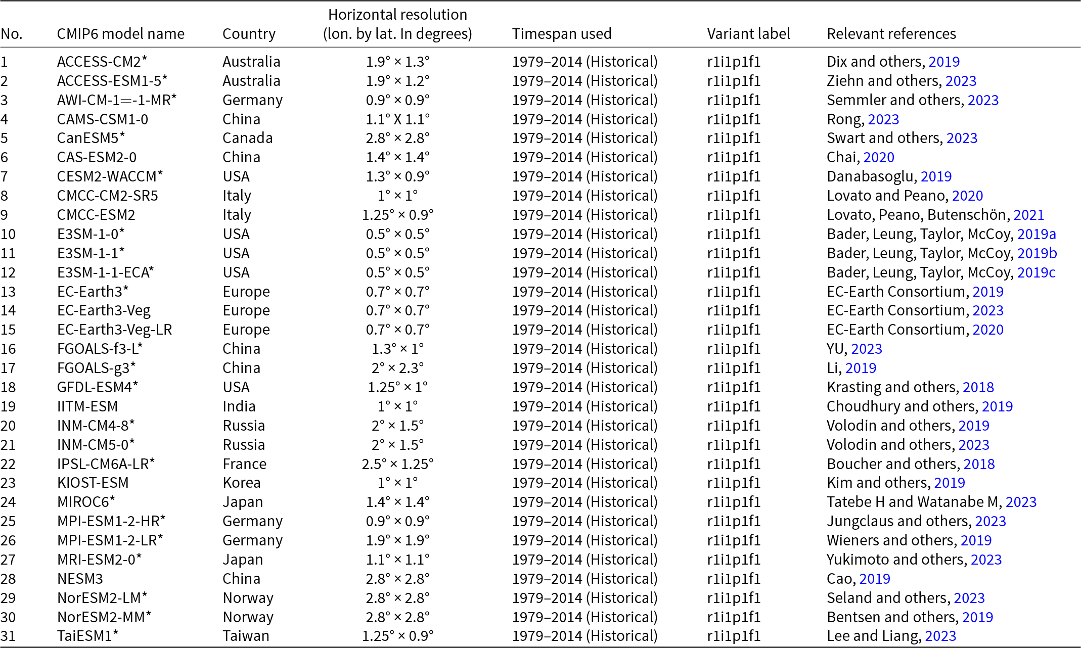
We chose 31 CMIP6 models, shown in Table 1 in Appendix A, from the Earth System Grid Federation (ESGF) (Cinquini and others, 2014), based on the availability of monthly temperature data for the time period 1979–2014 in the historical CMIP6 model runs, which cover the period (1850–2014).

To directly compare the ERA5 dataset with the CMIP6 models, we first interpolate the CMIP6 model outputs to ERA5 grid resolution (0.25° × 0.25°) using bilinear interpolation through the Climate Data Operator (CDO) for data regridding (Schulzweida, 2023). We select ice shelves for our analysis based on their size, ensuring that each can be represented by more than one grid cell at ERA5’s spatial resolution. The ice shelf boundaries for our analysis are sourced from MEaSUREs Antarctic Boundaries for IPY 2007–2009 from Satellite Radar, Version 2 (Rignot and others, 2013; Mouginot and others, 2017). Forty-six ice shelves meet our criteria, as illustrated in Fig. 1. We also tested regridding ERA5 to the native CMIP model resolution of 1° × 1°, which had no significant impact on the results. However, interpolating to the lower resolution of the CMIP6 models resulted in fewer ice shelves that met our selection criteria.

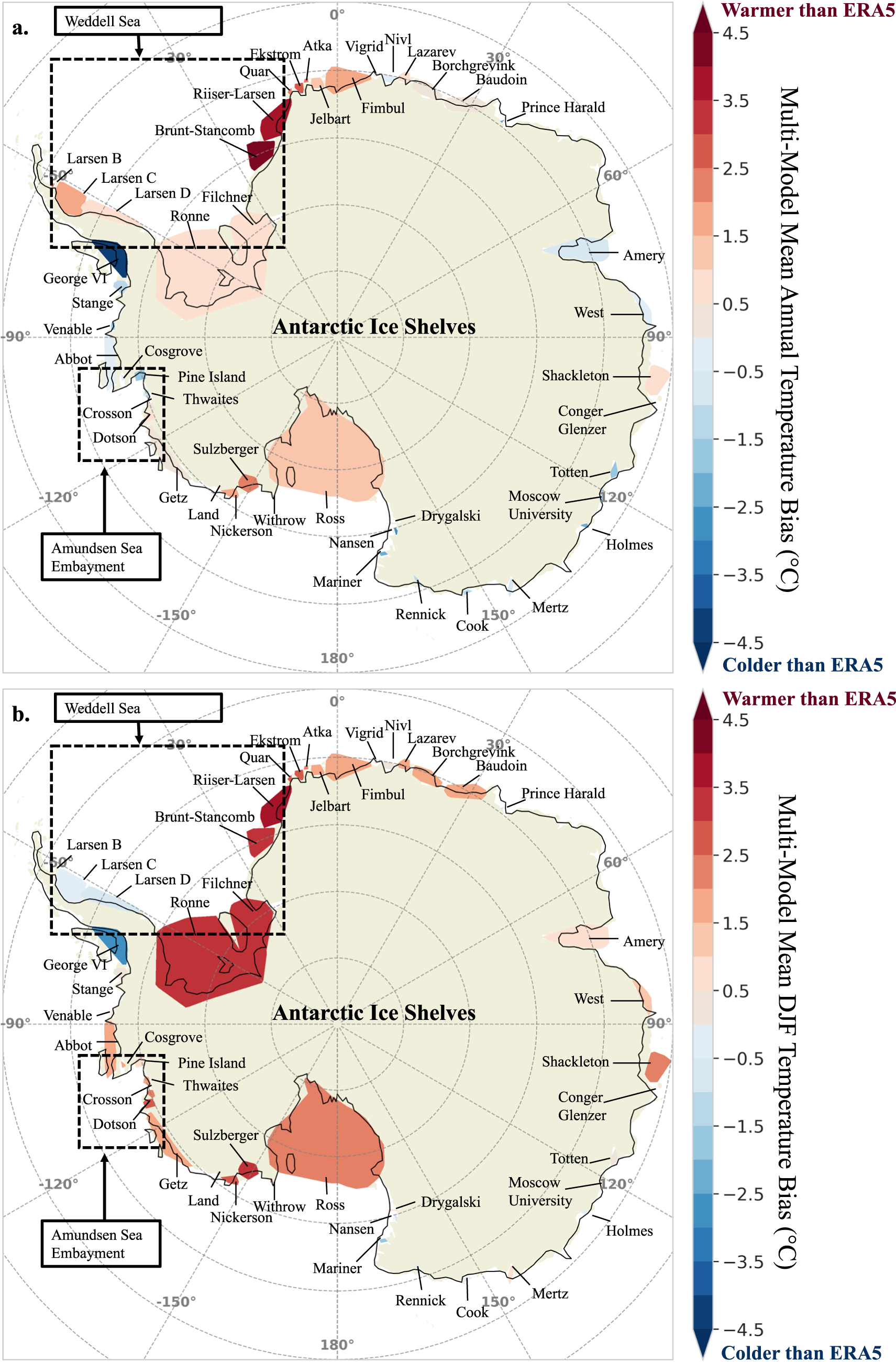
Figure 1. Multi-model mean near-surface air temperature, defined as the CMIP6 model near-surface air temperature minus ERA5’s near-surface air temperature, for 46 Antarctic ice shelves averaged over the period 1979-2014. (a) Annual multi-model mean near-surface air temperature bias. (b) Austral summer (DJF) multi-model mean near-surface air temperature bias. Colors indicate the degree of temperature over- or underestimation with respect to ERA5 on each ice shelf.

3. Methodology

We use two evaluation metrics to compare the CMIP6 models to ERA5: model bias and interannual variability measured through a standard deviation analysis. Model bias indicates whether models over—or underestimate mean atmospheric temperatures over ice shelves and is crucial to accurately determine when atmospheric temperatures consistently exceed proposed temperature thresholds. By contrast, the standard deviation measures how well models capture the average magnitude of interannual variability in atmospheric temperature. Both the temperature trend and the short-term fluctuations superimposed on it are important in triggering melt for ice shelves that are close to proposed surface melt thresholds when melt begins to appear (e.g. Morris and Vaughan, 2003; van Wessem and others, 2023). For example, the disintegration of Larsen B appears to have been driven by a short-term warming prior to collapse (Scambos and others, 2004; Turner and others, 2005; Leeson and others, 2017).

3.1. Model bias

Our approach for determining model bias involves comparing CMIP6 model near-surface air temperatures with ERA5 reanalysis data over Antarctic ice shelves from 1979 to 2014. We begin our analysis in 1979, as it is the beginning of the satellite era, providing more observational constraints for the ERA5 reanalysis. The end date of 2014 was chosen because this was the point where the CMIP6 models transitioned to using prescribed climate scenarios. We calculate mean monthly and seasonal differences, focusing on two temporal scales: the austral summer (December–January–February, DJF) and annual temperature bias (average over all months), because parameterizations of surface melt have traditionally invoked these two time scales. To calculate averages for individual ice shelves, we compute the spatial average of annual and austral summer temperature biases across all grid cells contained within each individual ice shelf. We calculate the averages for all ice shelves combined by computing the spatial average across all grid cells that are contained by one or more ice shelves. The DJF bias is important because it is Antarctica’s warmest season when most of the surface melt occurs (de Roda Husman and others, 2024). We also examine the annual temperature bias because several proposed surface melt thresholds in the literature use annual temperatures (e.g. Morris and Vaughan, 2003; van Wessem and others, 2023). To calculate the bias, we used the following steps:

1. 1. Interpolate the CMIP6 model output to a 0.25° × 0.25° ERA5 grid.

2. 2. Apply ice shelf boundaries to mask all interpolated CMIP6 or ERA5 reanalysis grid cells that are not identified as ice shelves.

3. 3. Calculate the monthly near-surface air temperature bias values for each grid cell associated with the ice shelves. The near-surface air temperature bias is defined as the difference between the CMIP6 model near-surface air temperature and ERA5’s near-surface air temperature.

4. 4. Calculate the temporal average of the monthly near-surface air temperatures over all months to calculate the mean annual bias, and the temperature over DJF to estimate the mean DJF bias.

5. 5. Compute the spatial average of the temperature bias for all grid cells on each ice shelf, which we refer to as the annual and DJF near-surface air temperature bias.

6. 6. Finally, we compute a spatial average of all the grid cells across the 46 ice shelves we analyze in this study to calculate the average annual and DJF near-surface air temperature bias for each CMIP6 model.

Steps (1–5) yield ice shelf-averaged annual and DJF near-surface air temperature biases for each of the 31 CMIP6 models over each of the 46 ice shelves analyzed in our study. The results from Step 6 provide an estimate of the average model performance across all ice shelves but are skewed towards model performance over the largest ice shelves, such as Ross, Filchner and Ronne. Alternatively, the results from Step 5 allow us to examine individual CMIP6 model performance over individual ice shelves.

Additionally, we calculated the multi-model mean near-surface air temperature biases for each ice shelf and averaged them over all ice shelves. We averaged the biases for all CMIP6 models after step (5) to obtain the ice shelf-averaged annual and DJF multi-model mean near-surface air temperature bias and then the annual and DJF multi-model mean near-surface air temperature bias averaged over all ice shelves.

3.2. Interannual variability

In addition to assessing biases, we examined the ability of the models to capture annual near-surface air temperature variability through a standard deviation analysis. The standard deviation quantifies a CMIP6 model’s intra-model variability of atmospheric near-surface air temperature, which we compare to ERA5’s variability. We first compute the spatial average of near-surface air temperature across all ice shelves from 1979 to 2014, and then calculate the temporal mean for both the annual and austral summer (DJF) periods. We then calculate the standard deviation of the resulting annual and DJF time series for each CMIP6 model, yielding a single value that represents the interannual variability in spatially averaged near-surface air temperature across all ice shelves. This approach allows us to quantify interannual variability for both the annual and austral summer periods, consistent with the method used in previous studies (Giorgi and Bi, 2005). Similarly, we computed the standard deviation of ERA5’s annual and DJF near-surface air temperatures for the same period. By comparing the standard deviations, we can assess how well the CMIP6 models capture the natural temperature variability over Antarctic ice shelves.

3.3. Statistical significance

To determine the statistical significance of the multi-model mean biases across the Antarctic ice shelves, we performed normality testing via the Shapiro–Wilk test (Shapiro and Wilk, 1965) for both the annual and DJF near-surface air temperature time series from 1979 to 2014. We find that both annual and DJF time series are non-normal and skewed, primarily due to long-term warming trends in both CMIP6 models and ERA5. Therefore, we used the non-parametric Mann–Whitney U test (Mann and Whitney, 1947) to assess if the multi-model mean differs significantly from ERA5, adopting a 95% confidence threshold (p ≤ 0.05). Similarly, we employed the Fligner–Killeen test (Fligner and Killeen, 1976) to assess the statistical significance of differences in interannual variability, as this non-parametric test is robust to deviations from normality. Significance was again evaluated at the 95% confidence level (p ≤ 0.05).

4. Results

4.1. Multi-model mean bias

We assessed the multi-model mean near-surface air temperature bias in annual and austral summer (DJF) time periods for 46 Antarctic ice shelves over the 1979–2014 period (Fig. 1).

4.1.1. Annual bias

Spatially, the annual multi-model mean bias (Fig. 1a) reveals substantial variation among shelves. Warm biases exceeding 3°C are evident for Brunt-Stancomb, Riiser-Larsen, and Sulzberger, while shelves such as Abbot, West, and Nivl exhibit comparatively small biases. East Antarctic ice shelves generally have biases between −2°C and 2°C, whereas those in West Antarctica exhibit a broader range, from −4°C to 5°C. Notably, the two largest ice shelves, Ronne and Ross, each present warm biases greater than 2°C, whereas Amery, situated in East Antarctica, has an annual mean bias near zero.

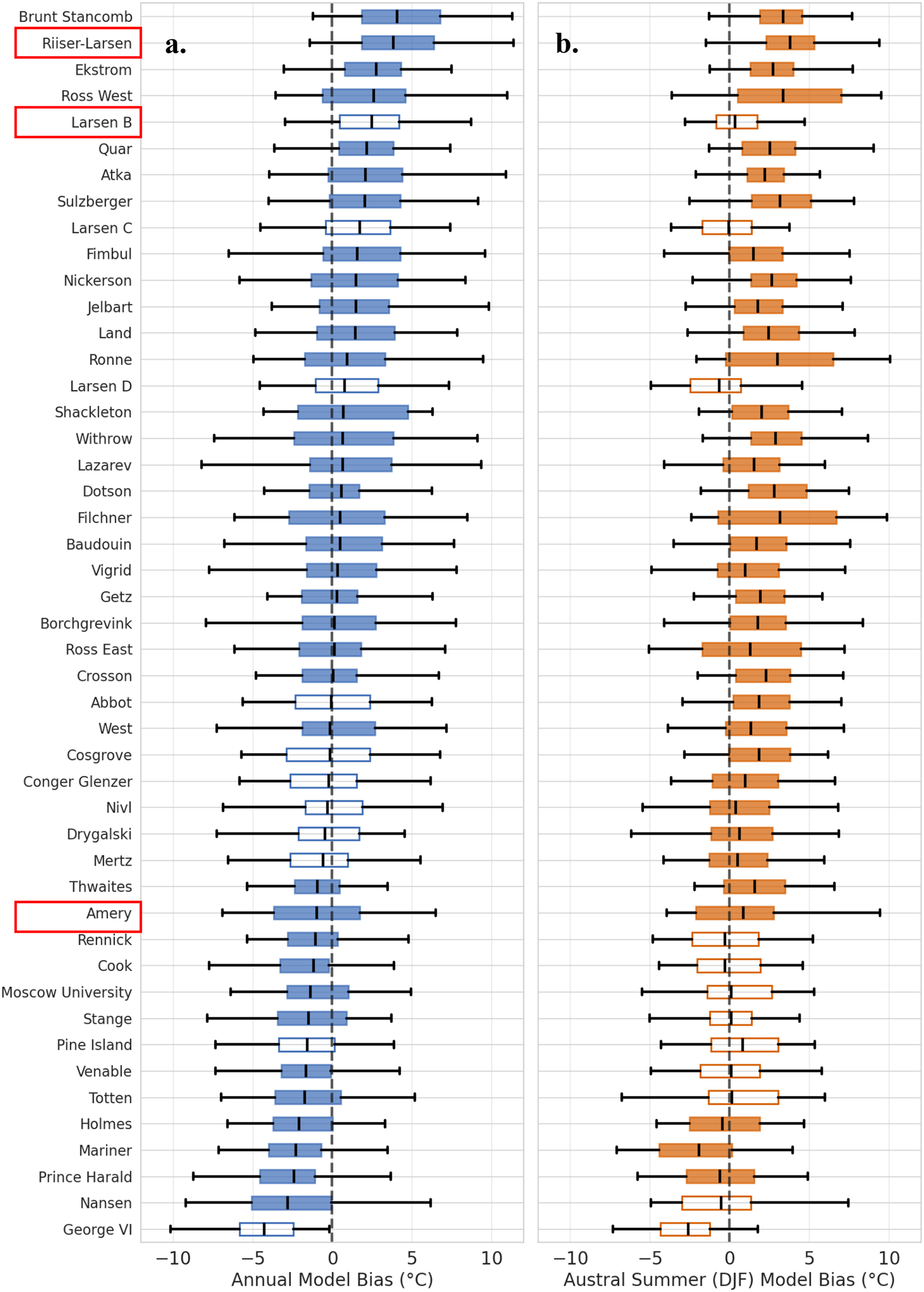
Results of the Mann–Whitney U test for the annual and DJF near-surface air temperature time series for the 46 shelves are summarized in Table S1 and Table S2 in the Supplementary Information (SI). Shelves where the multi-model mean bias is not statistically significant are marked by unfilled boxes in Fig. 2; almost 87% (40 out of 46) of shelves have a significant annual multi-model mean bias (Fig. 2a).

Figure 2. Box-and-whisker plots illustrating the distribution of near-surface air temperature biases for 31 CMIP6 models, relative to ERA5, spatially averaged over 46 ice shelves (with Ross divided into Ross East and Ross West) over the period 1979–2014. Panel (a) shows annual near-surface air temperature biases from CMIP6 models (shown in blue), while panel (b) displays austral summer (DJF) biases (shown in Orange) for each ice shelf. Each box represents the interquartile range (IQR), with the CMIP6 multi-model mean indicated by a horizontal line inside the box, and whiskers extending to the most extreme values within 1.5 × IQR. Filled boxes and whiskers indicate shelves where the CMIP6 multi-model mean bias is statistically significant compared to ERA5 (Mann–Whitney U test); unfilled boxes and whiskers indicate shelves where the bias is small or not significant. The vertical dashed line denotes zero bias in the multi-model mean. The red boxes indicate the ice shelves we will explore in more detail in Section 4.3.

4.1.2. Austral summer (DJF) bias

Because DJF near-surface air temperatures may better reflect melt pond formation, we next examined the multi-model mean December–January–February (DJF) biases for each ice shelf (Fig. 1b). We find even more pronounced warm biases in comparison to the annual biases shown in Fig. 1a: 28 out of 46 shelves experience multi-model DJF biases exceeding 1°C, including the Ronne-Filchner, Ross, and Amery shelves. As with the annual means, the largest warm DJF biases appear on Brunt-Stancomb, Riiser-Larsen, and Sulzberger.

Nonetheless, some shelves diverge from their annual behavior. For example, the Amundsen Sea Embayment (black dashed box in Fig. 1a) ice shelves transition from an annual cold bias to a DJF warm bias. On the Antarctic Peninsula, the Larsen shelves (east side) are annually warm-biased but become cold-biased in DJF, while George VI and Stange (west side) maintain significant cold biases across both periods. Statistically, 83% (38 out of 46) of shelves display significant DJF multi-model mean near-surface air temperature biases when compared to ERA5, which is visually reflected by the filled orange boxes in Fig. 2b.

Although the multi-model mean provides a useful summary of overall CMIP6 model tendencies and reveals regional patterns in annual and DJF biases across the Antarctic ice shelves, it can mask substantial differences among individual models. In practice, we typically select subsets of CMIP models to drive ice sheet-shelf projections, and some CMIP6 members may perform notably better (or worse) over certain shelves. In some cases, the multi-model mean bias may be influenced by the presence of outlier models, as suggested by the error bars in Fig. 2. To explore these possibilities, we further assess the performance of individual CMIP6 models over ice shelves in Sections 4.2 and 4.3.

4.2. Performance of individual CMIP6 models averaged over all shelves

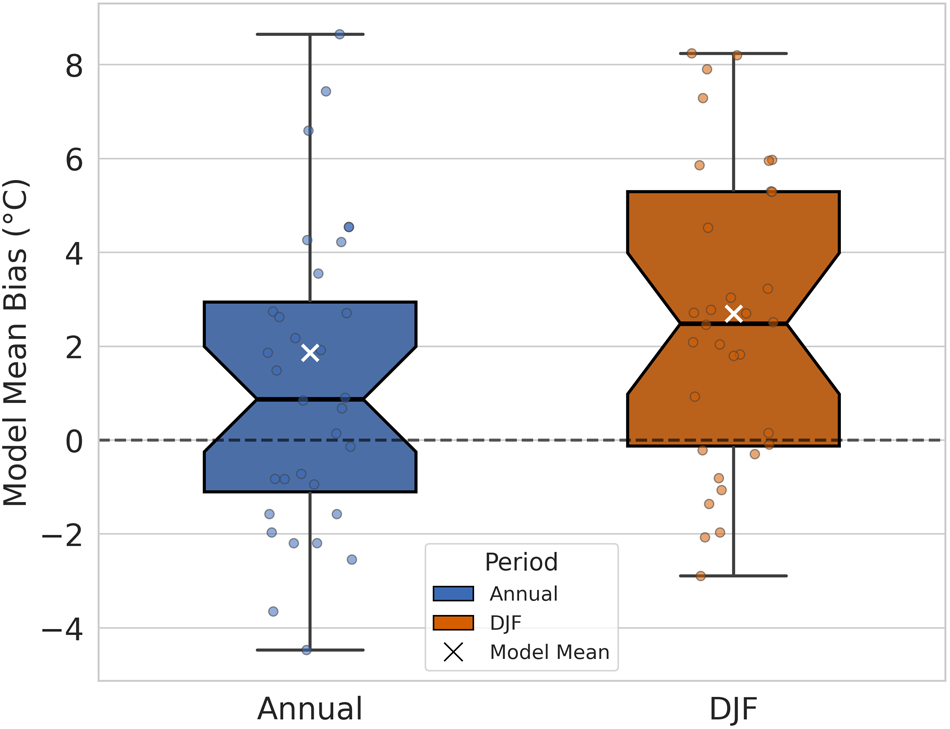
Recognizing the potential for both outlier influence and varying model performance, we now focus on individual CMIP6 model near-surface air temperature biases spatially averaged across all 46 ice shelves and averaged across the period 1979 to 2014. Figure 3 summarizes the distribution of spatially averaged near-surface air temperature biases across 31 CMIP6 models alongside the multi-model mean, for both annual and austral summer (DJF). The box-and-whisker plot highlights a clear tendency toward warm biases across the CMIP6 models, with the bulk of model biases (the interquartile range) clustering between 0°C and 2°C above the ERA5 reference (0°C bias line) for both annual and summer means. This systematic warm bias is particularly pronounced during the austral summer, as seen by the higher median and a larger proportion of models lying above the zero-bias line.

Figure 3. Box-and-whisker plots showing the distribution of near-surface air temperature biases for 32 models, including 31 CMIP6 models and the multi-model mean, relative to ERA5, spatially averaged across all Antarctic ice shelves and averaged over the period 1979–2014. The model points have been jittered from a single line to visualize each of the different models within the box-and-whisker plots. The left panel displays annual (blue) mean near-surface air temperature biases, while the right panel shows austral summer (DJF) (Orange) biases. Each point represents an individual model, and the multi-model mean is represented by a white X. Boxes indicate the interquartile range (IQR), the median is marked by a horizontal line within each box, and whiskers extend to the most extreme values within 1.5 × IQR.

The vertical extent of the boxes and whiskers, in Fig. 3 reveal substantial inter-model variability: some models underestimate temperatures by more than 4°C, while others overestimate by up to 8°C annually. The wide range in the whiskers substantiates the observation that although the majority of CMIP6 models overestimate near-surface air temperatures, there is considerable diversity in model performance, with a few models exhibiting notable cold biases as well.

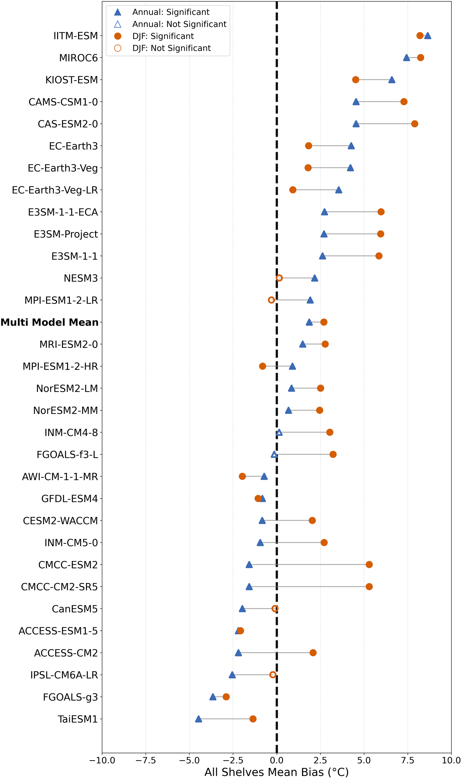
To further clarify individual model performance and model-to-model differences, Fig. 4 presents the annual and DJF mean near-surface air temperature biases for each CMIP6 model and the multi-model mean averaged across all ice shelves. Using this approach, we find that 87.5% (28 out of 32) of models exhibit a statistically significant bias annually, and almost 94% (30 out of 32) of models have a statistically significant bias during DJF (Fig. 4). Moreover, most models maintain their bias sign (either warm or cold) across the annual and austral summer periods, supporting the earlier observation of persistent model tendencies. However, several models exhibit shifts in bias direction or large changes in bias magnitude, underscoring the diversity of responses among models. For example, the CMCC-ESM2 model exhibits a cold annual temperature bias, but a warm DJF temperature bias, indicating strong seasonal patterns.

Figure 4. Pairwise comparison of near-surface air temperature biases for individual CMIP6 models (and the multi-model mean) with respect to ERA5, averaged across all Antarctic ice shelves and weighted by ice shelf area for the period 1979–2014. For each model, mean annual bias (blue triangles) and austral summer (DJF) bias (Orange circles) are shown, with lines connecting the two for each model to illustrate consistency or changes in seasonal bias. Filled symbols indicate models for which the bias is statistically significant compared to ERA5 (using the Mann–Whitney U test), while open symbols denote comparably small or non-significant biases. The vertical dashed line represents zero mean bias across all shelves.

Although our analysis provides insights into the model performance averaged across all ice shelves, it raises questions about potential variations in model performance between individual ice shelves. To address this limitation and gain a more comprehensive understanding of model performance across different Antarctic locations, we examine specific case studies, including the Larsen B, Amery, and Riiser-Larsen ice shelves. These case studies allow us to examine the regional variations of the CMIP6 models’ representation of diverse Antarctic environments in greater detail.

4.3. Comparison of CMIP6 model performance over the Larsen, Amery, and Riiser-Larsen ice shelves

To further illustrate inter-model variability and regional differences in CMIP6 model performance, we compare the near-surface air temperature biases over three representative ice shelves: Larsen B on the Antarctic Peninsula, Amery in East Antarctica and Riiser-Larsen in West Antarctica, as shown in Figs. 5 and 6. These figures provide complementary perspectives on model spread, mean tendencies, and pairwise differences for these shelves.

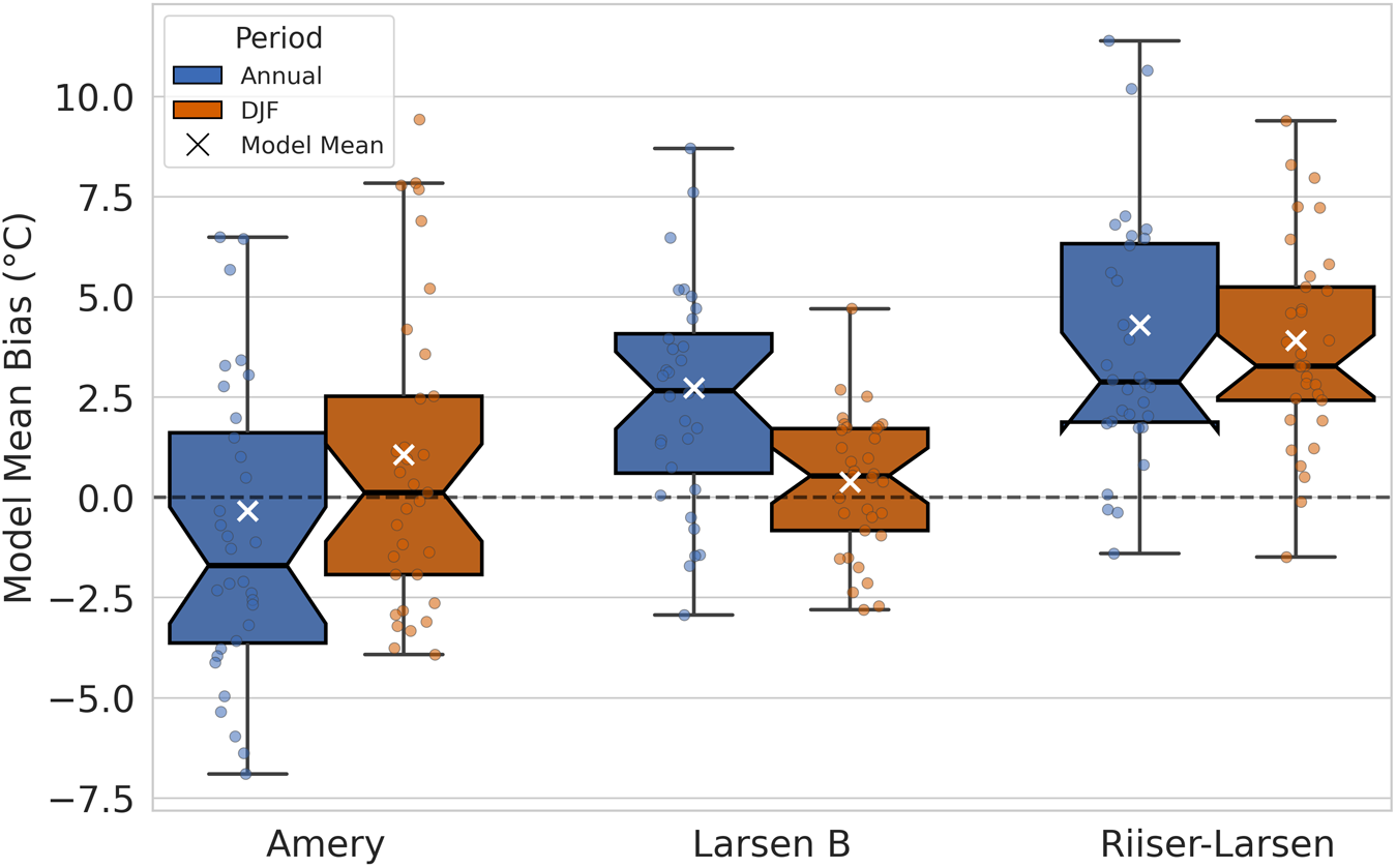
Figure 5. Box-and-whisker plots showing the distribution of near-surface air temperature biases for the annual (blue) and austral summer (Orange) averaged over the period 1979–2014 for 32 models, including 31 CMIP6 models and the multi-model mean, relative to ERA5, over the Amery, Larsen B, and Riiser-Larsen ice shelves. The model points have been jittered from a single line to visualize each of the different models within the box-and-whisker plots. Each point represents an individual model, and the multi-model mean is represented by a white X. Boxes indicate the interquartile range (IQR). The median is marked by a horizontal line within each box, and whiskers extend to the most extreme values within 1.5 × IQR.

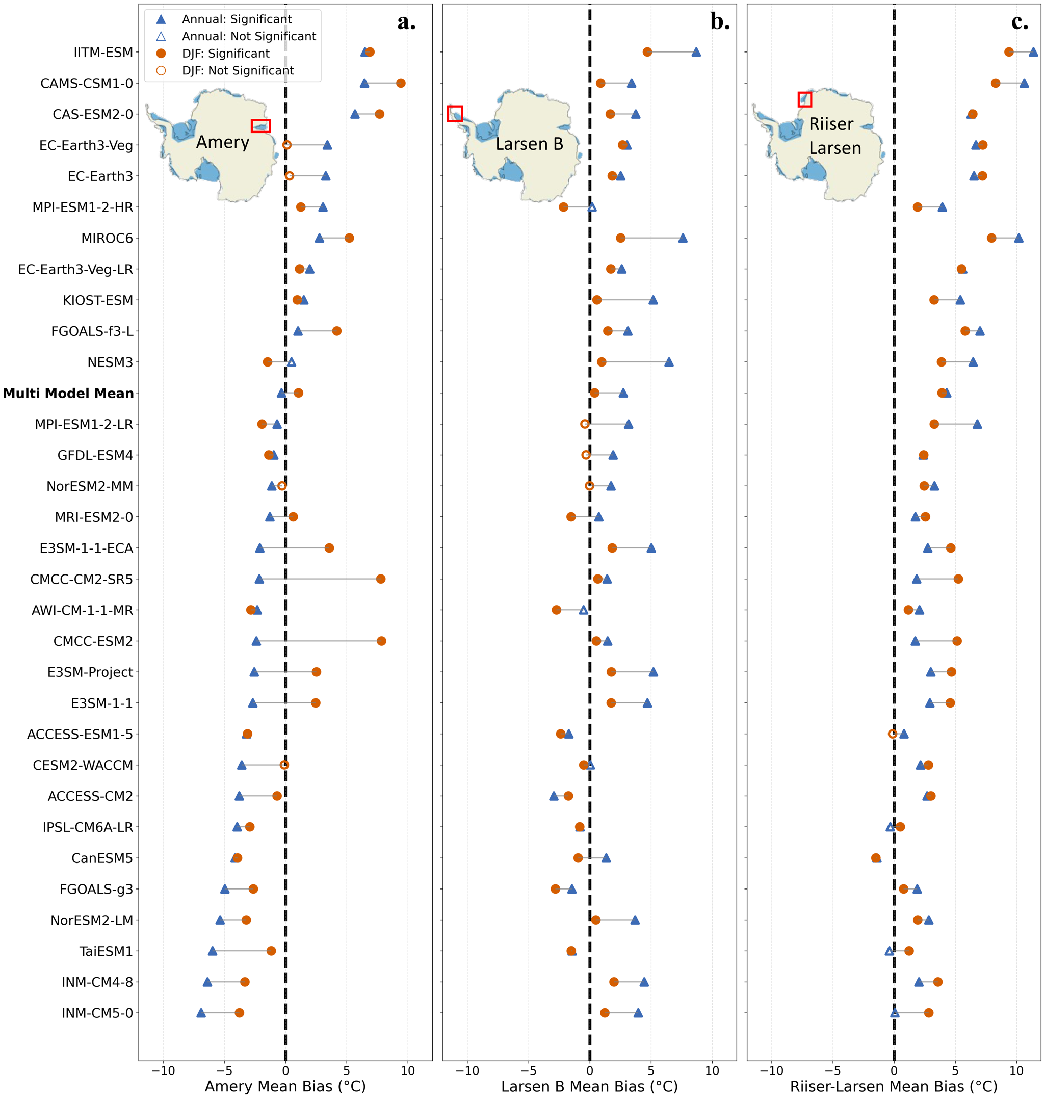
Figure 6. Pairwise comparison of near-surface air temperature biases for individual CMIP6 models (and the multi-model mean) with respect to ERA5, averaged over the period 1979–2014 for the a) Amery, b) Larsen B, and c) Riiser-Larsen ice shelves. For each model, mean annual bias (blue triangles) and austral summer (DJF) bias (Orange circles) are shown, with lines connecting the two for each model to illustrate consistency or changes in seasonal bias. Filled symbols indicate models for which the bias is statistically significant compared to ERA5 (using the Mann–Whitney U test), while open symbols denote comparably small or non-significant biases. The vertical dashed line represents zero mean bias.

Figure 5 displays box and whisker plots showing the distribution of near-surface air temperature biases—both annually and for the austral summer (DJF)—over the Amery, Larsen B, and Riiser-Larsen ice shelves. Each boxplot summarizes results from 31 CMIP6 models and the multi-model mean, all referenced to ERA5. Annual mean biases (blue) and DJF biases (orange) are shown separately, with each point representing an individual model.

Riiser-Larsen stands out for its pronounced warm bias in the CMIP6 models: most models have annual and summer biases above the ERA5 reference (0°C), with the medians of both distributions exceeding 2.5°C. Similarly, for Larsen B, most model biases are positive, with a median annual bias around 2.5°C and a slightly lower median DJF bias just above zero. Both Riiser-Larsen and Larsen B highlight a widespread tendency for models to overestimate near-surface air temperatures near the Antarctic Peninsula and Weddell Sea.

In contrast, the Amery ice shelf presents a more nuanced pattern. The annual bias distribution shows that about 66% (20 out of 31) of models have a cold bias, but there is a large spread in model estimates—reflected in an interquartile range spanning roughly 13°C—indicating little consensus among models for this region. Despite similarly broad interquartile ranges for Larsen B (about 11°C) and Riiser-Larsen (about 12°C), most model results for these two shelves are clustered above 0°C. During DJF, all three shelves are predominantly warm-biased. Notably, Larsen B shows a narrower interquartile range in DJF, signifying greater agreement among models during the summer, whereas Amery and Riiser-Larsen maintain wide spreads, reflecting persistent inter-model variability similar to the annual results.

Figure 6 illustrates the pairwise, model-specific comparison for the Amery (panel a), Larsen B (panel b), and Riiser-Larsen (panel c), allowing a direct assessment of whether models that perform well for one ice shelf yield similar results elsewhere. As in Figs. 2 and 4, we determined the statistical significance of the near-surface air temperature biases relative to ERA5 using the Mann-Whitney U test, with results summarized in Tables S5-S10 of the Supplementary Information (SI).

Figure 6 demonstrates that model performance is inconsistent across shelves. For example, the CMCC-ESM2 model shows a dramatic shift over Amery (from −2°C annually to 7.6°C in DJF), while the change between periods on Larsen B and Riiser-Larsen is less pronounced (within 4°C). NESM3 performs well over Amery annually (with its bias not statistically significant), but shows a ∼6°C warm bias during the annual period for both Larsen B and Riiser-Larsen. Similarly, the CESM2-WACCM model has relatively small biases over Larsen B, but exhibits a substantial cold bias (about −4°C) on Amery and a 2.5°C warm bias on Riiser-Larsen.

These findings suggest that relying on the multi-model mean, or assuming that good performance in one region translates to similar skill elsewhere, can overlook significant differences in model performance across shelves. The distributions of CMIP6 model biases (Fig. 5) and the pairwise model comparisons (Fig. 6) reinforce the need to evaluate and select models according to the specific objectives and regional focus of an ice shelf projection study.

4.4. Ability of CMIP6 models to reproduce interannual variability

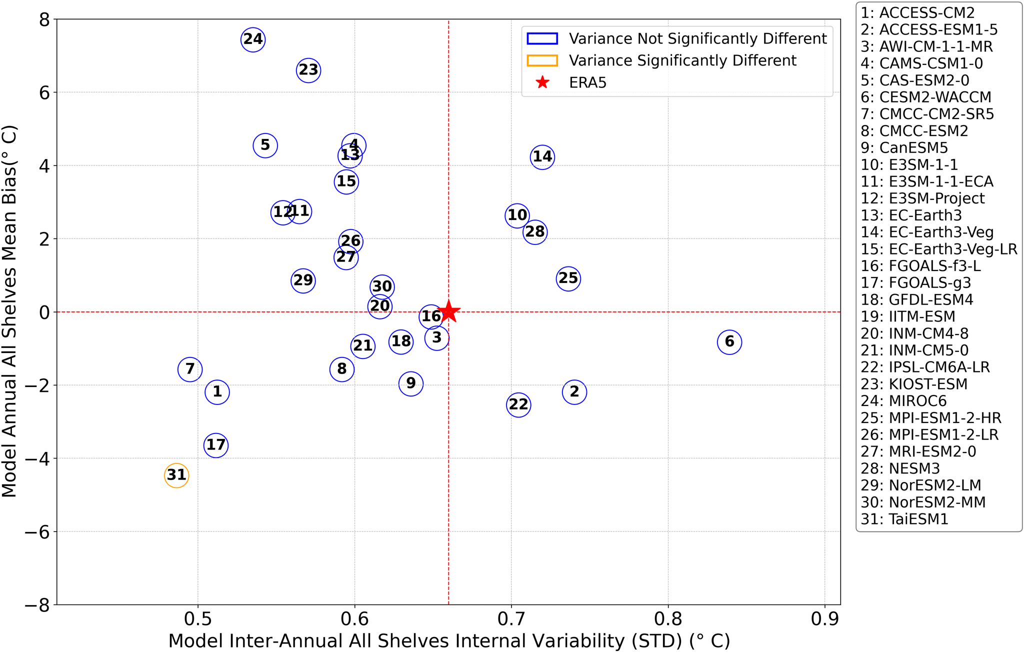
Analysis of the CMIP6 model biases revealed significant inter-model variability and variation in individual model performance between ice shelves. To further evaluate model performance, we examined the interannual variability of the near-surface air temperature in each CMIP6 model relative to ERA5, using standard deviation as a metric. Figure 7 presents the relationship between interannual variability (standard deviation) and the spatially averaged near-surface air temperature bias across all ice shelves, for each CMIP6 model (displayed as blue and orange circles) and ERA5 (displayed as a red star).

Figure 7. Scatter plot showing the interannual variability and bias of near-surface air temperature for CMIP6 models, averaged across all ice shelves for the period 1979–2014. The x-axis represents model interannual variability, quantified as the standard deviation of temperature, while the y-axis shows the mean annual near-surface air temperature bias relative to ERA5, averaged across all ice shelves. Each blue circle with a black number corresponds to a CMIP6 model whose variance is not statistically different from ERA5 according to the Fligner-Killeen test. In contrast, each Orange circle indicates a model with a statistically significant difference in variance. The black numbers within the circles refer to the model numbers listed in the legend to the right of the plot. The standard deviation of ERA5’s annual near-surface air temperature, averaged across all ice shelves, is indicated by a red star. For reference, two dashed red lines are included: one horizontal line at zero on the y-axis, indicating ERA5’s zero bias with respect to itself, and one vertical line at the ERA5 standard deviation on the x-axis, facilitating a direct comparison of model variability with ERA5.

As previously discussed, the spatially averaged CMIP6 model near-surface air temperature series from 1979 to 2014 are not normally distributed. Accordingly, we employed the Fligner-Killeen test (Fligner and Killeen, 1976) to assess the statistical significance of differences in interannual variability. Significance was evaluated at the 95% confidence level (p ≤ 0.05). Results of the Fligner-Killeen test for the spatially averaged annual near-surface air temperatures averaged across all ice shelves are detailed in Table S3 in the SI.

All but one CMIP6 model exhibit interannual variability (standard deviation) that is not statistically different from ERA5, as indicated by the blue and orange circles in Fig. 7. Only TaiESM1 (labeled ‘31’ in Fig. 7) displays significantly different interannual variability, with a smaller standard deviation than both ERA5 and the other models.

Despite the wide range of temperature biases among CMIP6 models (from approximately −4°C to +8°C), most models do not differ significantly from ERA5 in terms of the magnitude of their interannual variability. This result suggests that, following appropriate bias correction, many CMIP6 models may offer valuable projections for future climate conditions over Antarctic ice shelves, although some models exhibit larger or smaller variability that may be interesting to probe even if not statistically significant.

4.5. Exploring the role of surface orography and land/ice area fraction in near-surface air temperature biases

Although some models display large biases, it is possible that these are merely a consequence of low resolution or inaccurate surface orography or different methods of prescribing ice area fraction. If a model’s surface orography is higher than that in the ERA5 product, it could lead to a cold temperature bias; conversely, lower elevations may result in a warm bias. Additionally, temperature biases may arise from the misclassification of ice as ocean in the model, particularly over smaller ice shelves. This misclassification can lead to artificially warm conditions in regions where ice coverage is underestimated.

4.5.1. Does land ice area fraction control the observed near-surface air temperature bias?

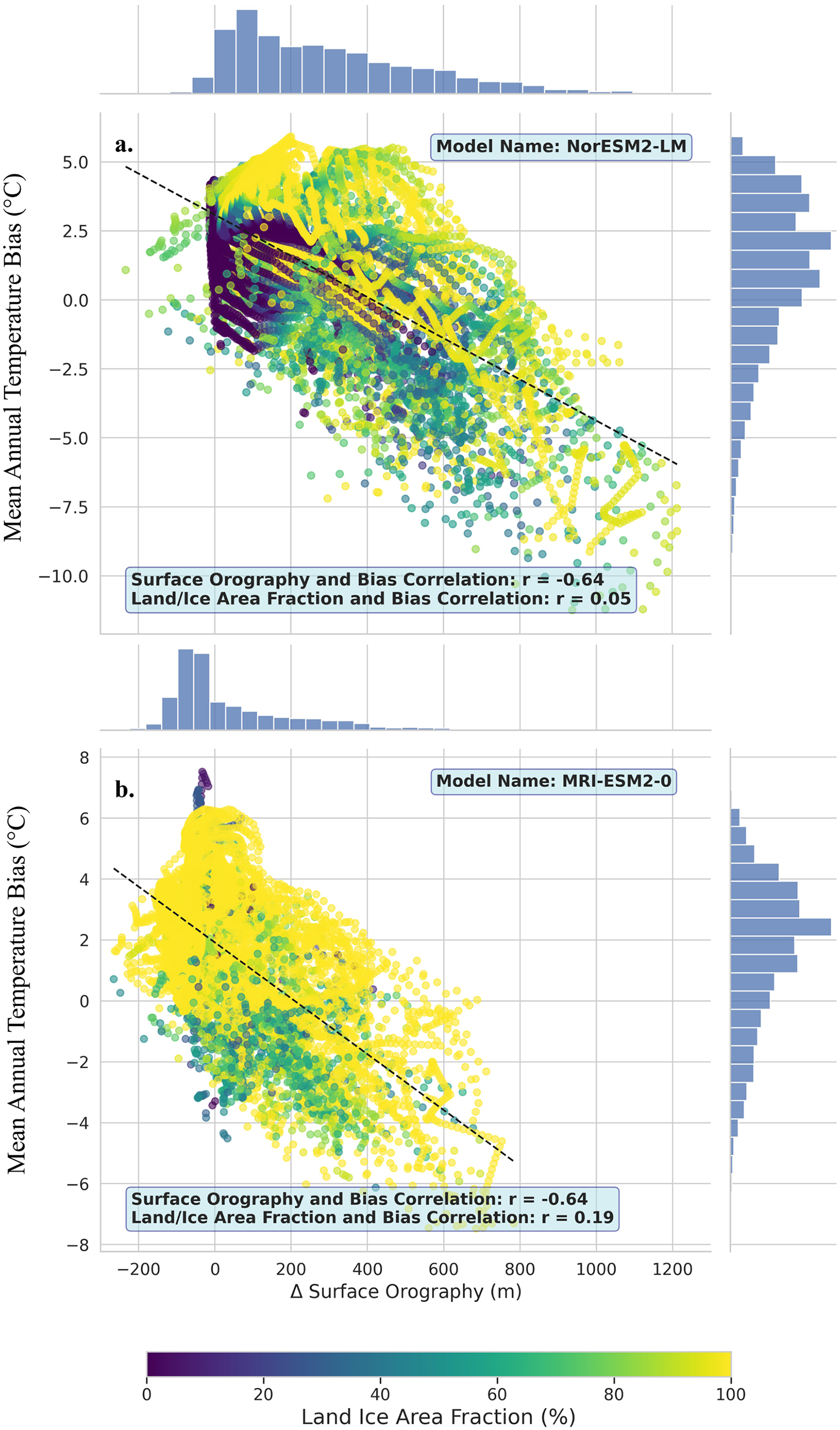
In a CMIP6 model, the land ice area fraction describes the fraction of a grid cell occupied by ‘permanent’ ice, which includes glaciers, ice caps, ice sheets and ice shelves (Taylor and others, 2007). To illustrate the role of land ice area fraction in controlling bias, we analyzed 11 CMIP6 models with available land ice area fraction and surface orography data. We focus on two models, NorESM2-LM and MRI-ESM2-0, as examples of models with similar annual warm near-surface air temperature biases averaged across all ice shelves, 1.5°C and 1.8°C, respectively. Figure 8 displays the percentage of land ice area fraction for each ice shelf grid cell (displayed using the color of the scattered points in both Figs. 8a and 8b) against the annual near-surface air temperature bias (y-axis) and surface orography difference (x-axis) for NorESM2-LM (Fig. 8a) and MRI-ESM2-0 (Fig. 8b).

Figure 8. The scatter plot depicts the relationship between changes in surface orography and annual near-surface air temperature biases for 9716 grid cells (0.25° × 0.25° resolution) across 46 Antarctic ice shelves, comparing (a) the CMIP6 model NorESM2-LM to ERA5 reanalysis data and (b) the CMIP6 model MRI-ESM2-0 to ERA5 reanalysis data. The x-axis represents the change in surface orography (in meters), which is defined as the CMIP6 model surface orography minus ERA5’s surface orography, while the y-axis shows the annual near-surface air temperature bias defined as the CMIP6 model temperature minus ERA5’s temperature. The scatter plot points are colored according to the land ice area fraction of the CMIP6 model, (a) NorESM2-LM and (b) MRI-ESM2-0, with lighter points representing a higher percentage of land ice in a given grid cell. The histogram on the right side of Figs. 8a and 8b illustrates the density of points for the annual near-surface air temperature bias for the CMIP6 model, whereas the histogram on the top of Figs. 8a and 8b displays the density of points for the change in surface orography for the CMIP6 model.

Our analysis revealed no clear correlation between land ice area fraction and annual near-surface air temperature bias for both NorESM2-LM (correlation coefficient: 0.05, Fig. S1a) and MRI-ESM2-0 (correlation coefficient: 0.19, Fig. S1b). For example, we identified a selection of grid boxes in the top left corner of Figs. 8a and 8b that have a high land ice area fraction but a high mean annual temperature bias, suggesting that the land ice area fraction does not control the bias in NorESM2-LM or MRI-ESM2-0.

Extending our analysis to all 11 CMIP6 models, we calculated average correlations between land ice area fraction and near-surface air temperature biases. The average correlation between the land ice area fraction and near-surface air temperature biases is −0.18 ± 0.24 (range: −0.5–0.21). These results demonstrate significant variation in the relationships between land ice area fraction and near-surface air temperature biases across models. Although we cannot generalize to all models, our analysis suggests that near-surface air temperature bias is unlikely to be attributable solely to land-ice area fraction.

4.5.2. Does surface orography control the observed near-surface air temperature bias?

Alternatively, it is also possible that the near-surface air temperature biases in the CMIP6 models are related to the orography used in the models. Therefore, we examined the relationship between surface orography and near-surface air temperature biases across 46 ice shelves, analyzing 9716 grid cells at 0.25° × 0.25° resolution. For each grid cell, we calculated the difference between CMIP6 and ERA5 surface orography: negative values indicate lower orography in the CMIP6 model, while positive values reflect higher model orography relative to ERA5. We then assessed the correlation between this orography difference and annual near-surface air temperature bias for 22 CMIP6 models with available data (denoted by a * in Appendix A).

As illustrated in Fig. 8, NorESM2-LM and MRI-ESM2-0 display strong negative correlations (−0.64), indicating that higher model elevations are associated with increased cold biases. While these two models exhibit similar correlation strengths, the broader inter-model range is substantial. For example, GFDL-ESM4 displays a weaker, slightly positive correlation (0.28), which reflects an unphysical lapse rate. On average, the correlation coefficient across the 22 models is −0.33 ± 0.31 (range: −0.69–0.28). Only eight models (Nor-ESM2-LM, MRI-ESM2-0, E3SM-1-0, E3SM-1-1, E3SM-1-1-ECA, MIROC6, INM-CM5-0, and INM-CM4-8) yield plausible lapse rates, between the moist-adiabatic lapse rate of 5°C/km and the dry-adiabatic lapse rate 9.8°C/km for Antarctica (Feulner and others, 2013). This suggests that orography-related temperature biases might be partially corrected in these models with elevation adjustments, whereas the presence of unphysical lapse rates in other models points to the need for more complex, model-specific approaches.

4.5.3. Correcting the near-surface air temperature for observed differences in surface orography

Motivated by the relationship between annual near-surface air temperature biases and surface orography shown in Fig. 8, we next applied an orography-based temperature correction to the eight models with plausible lapse rates. Following a method similar to Dutra and others (2020), we corrected the near-surface air temperature using the following relationship for each grid cell across all 46 ice shelves:

(1)\begin{equation}{T_{elevation\,correcte{d_i}}} = {T_{CMIP\,model,i}} + {\Gamma _{model}} \times \Delta {h_i}\end{equation}

where ${T_{CMIP\;model}}$ is the original CMIP6 model temperature for a given grid cell, $\Delta h$ is the change in surface orography between the CMIP6 model and ERA5 for a given grid cell, i represents a specific grid cell, and ${\Gamma _{\bmod {\text{el}}}}$ is the model lapse rate defined as,

(2)\begin{equation}{\Gamma _{\bmod {\text{el}}}} = \left( {\frac{{\Delta T}}{{\Delta SH}}} \right) = \left( {\frac{{{{\text{T}}_{{\text{CMIP}}}} - {{\text{T}}_{ERA5}}}}{{{\text{S}}{{\text{H}}_{CMIP}} - S{H_{ERA5}}}}} \right).\end{equation}

The lapse rate is the slope derived from the linear fit between the annual near-surface temperature and surface orography biases for a given CMIP6 model, as illustrated in Fig. 8. We applied equation (1) to correct the annual CMIP6 model temperatures for each of the 8 models with available surface orography and plausible lapse rates. Subsequently, we calculated the annual temperature biases across the 46 ice shelves using the elevation-corrected temperatures, following the methodology detailed in Section 3.1.

Before the orographic correction, the multi-model mean exhibits widespread warm biases relative to ERA5, with shelf-average near-surface air temperature biases ranging from −5°C to 4°C, and a mean bias of −1 ± 2°C (Fig. 9b). This bias pattern is broadly consistent with the results using all 31 CMIP6 models in Fig. 1a, but with slightly warmer values in the 8-model subset. East Antarctic shelves show biases shifting from −2°C to 2°C (31 models, Fig. 1a) to −4°C–0°C (models, Fig. 9b), while West Antarctic shelves shift from −4°C–5°C to −5°C–4°C. Notably, biases for shelves in the Weddell Sea (e.g. Ronne, Filchner, Brunt-Stancomb, Riiser-Larsen), Amundsen Sea (e.g. Pine Island, Thwaites, Crosson, Dotson), and Ross Sea increase by up to 2°C, but the overall spread of biases remains similar in West Antarctica.

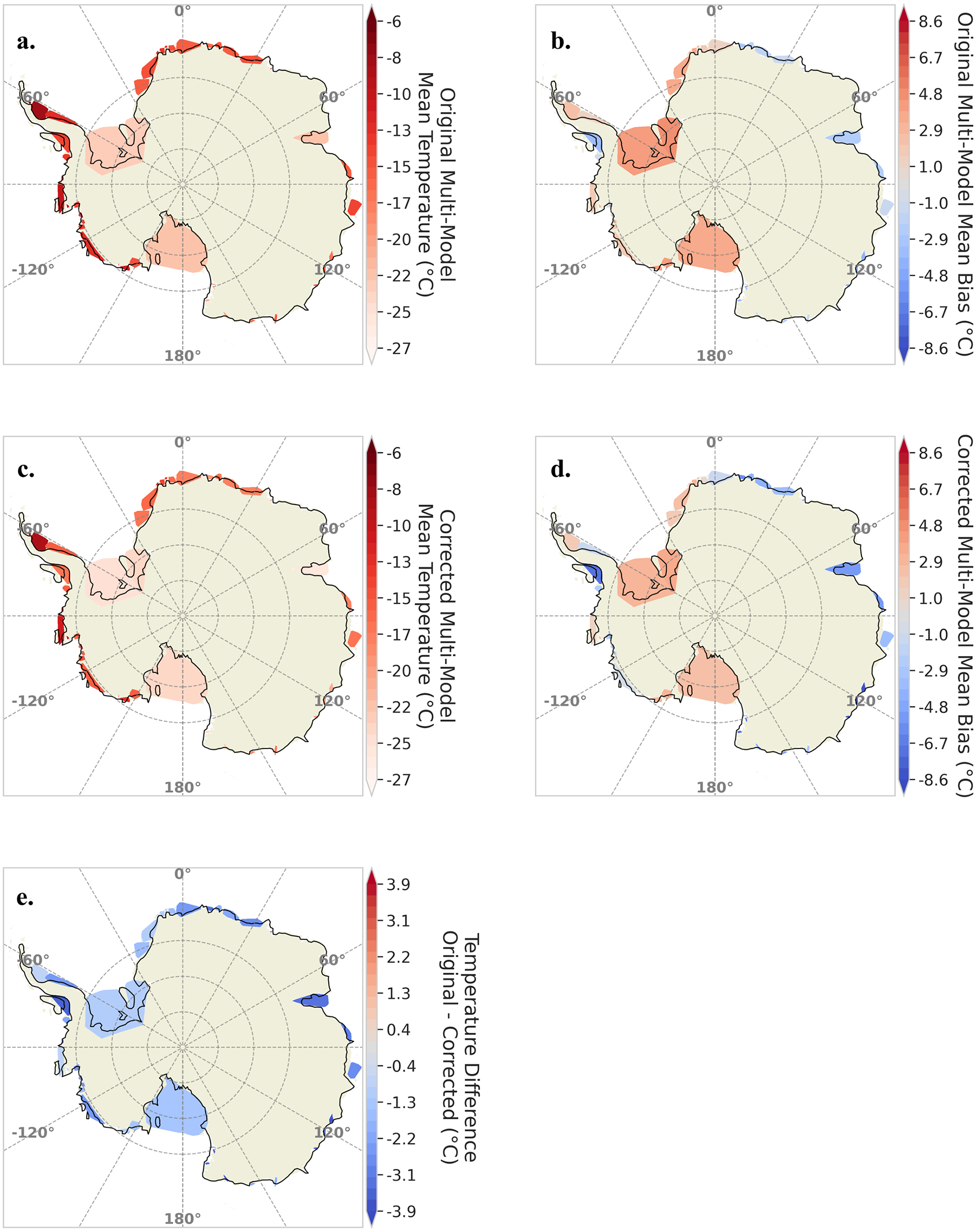
Figure 9. ERA5 mean annual near-surface air temperature compared to the multi-model mean near-surface air temperature for 46 Antarctic ice shelves using 8 out of the 31 CMIP6 (Nor-ESM2-LM, MRI-ESM2-0, E3SM-1-0, E3SM-1-1, E3SM-1-1-ECA, MIROC6, INM-CM5-0, and INM-CM4-8) models averaged over the period 1979-2014 before and after applying a lapse rate orographic correction. (a) The original multi-model mean near-surface temperature for the 8 CMIP6 models. (b) The annual mean near-surface air temperature bias for the original multi-model mean of the 8 CMIP6 models. Colors indicate the degree of temperature over- or underestimation on each ice shelf compared to ERA5. (c) The annual mean near-surface air temperature bias for the orography-corrected multi-model mean of the 8 CMIP6 models. Colors indicate the degree of temperature over- or underestimation on each ice shelf compared to ERA5. (d) The orography corrected multi-model mean near-surface temperature for the 8 CMIP6 models. (e) The temperature difference between the original multi-model mean and the orography corrected multi-model mean near-surface air temperature, defined as the original multi-model mean minus the orography corrected multi-model mean near-surface temperature, for the 8 CMIP6 models.

After applying the orographic correction (Fig. 9c/d), the range of model biases expands to −8°C–3°C (Fig. 9d), and the mean bias becomes slightly more negative at −2 ± 2°C (Fig. 9c). The average reduction in bias across all shelves is about 1 ± 0.5°C, with some regions experiencing a maximum change of 2°C (Fig. 9e). The four largest shelves—Ross, Ronne, Filchner and Amery—see an average bias reduction of 0.7 ± 0.5°C, while smaller shelves show a mean change of 1 ± 0.5°C.

Although the orographic correction reduces the warm biases on the ice shelves in the Weddell Sea (e.g. Ronne, Filchner, Brunt-Stancomb and Riiser-Larsen) and Ross Sea, it also shifts the overall bias pattern toward colder values rather than fully eliminating any systematic error. This likely reflects both the strengths and limitations of using a lapse rate correction based on fixed present-day orography: modest elevation differences have a limited effect, and changes in landscape through time cannot be captured with a static correction. This approach appears suitable for the historical period analyzed here, but may be less appropriate for future projections as the ice surface elevation changes. Additionally, the persistence of unphysical lapse rates in many models indicates that a simple linear adjustment may be insufficient, and more sophisticated approaches may be required for those models.

5. Discussion

Our analysis shows that CMIP6 models, overall, have a warm bias over Antarctic ice shelves broadly consistent with the global warm bias previously found for CMIP6 models (Fan and others, 2020; McKitrick and Christy, 2020; Scafetta, 2023). However, we also see substantial regional variations in the magnitude and sign of the bias. For example, Amundsen Sea Embayment ice shelves have a cold bias, whereas ice shelves in the Weddell Sea (e.g. Ronne, Filchner, Brunt-Stancomb and Riiser-Larsen) have a warm bias. Our study also emphasizes the large variations between individual CMIP6 model members, which can exceed $ \pm {13^ \circ }{\text{C}}$ for some ice shelves. Regionally, our analysis further reveals a pattern where smaller ice shelves, particularly along East Antarctica and in the Amundsen Sea Embayment, tend to exhibit cold biases, whereas larger ice shelves, such as those in West Antarctica, generally show warm biases.

The large variation in biases between models by ice shelf suggests that choosing the most appropriate CMIP6 model may depend on the specific research objective and the area of interest. For example, studies focused on surface melt on the Amundsen Sea Embayment ice shelves might prefer a different set of CMIP models from a study that looked at all ice shelves or a study focused on ice shelves in the Antarctic Peninsula. However, an important nuance to choosing a model based on our findings is that we focus exclusively on near-surface air temperatures over the ice shelves. Ocean forcing and snowfall, especially over the ice sheet, are also important climate drivers, and accounting for a wider array of atmospheric and oceanic forcing could provide additional context to model selection.

We further explored the relationship between the CMIP6 annual near-surface air temperature biases and variables such as surface orography and land/ice area fraction, finding that orographic differences may account for part of the observed biases, whereas the land/ice area fraction variable does not appear to be a major contributor. Nevertheless, the near-surface air temperature biases are likely multifactorial, with additional contributions from other mechanisms—such as biases in the upper atmospheric temperature, ocean surface temperature, sea ice extent, cloud cover and radiation, or atmospheric circulation—also likely contribute. Further investigation into these additional factors will be necessary to fully understand and address the persistent near-surface air temperature biases in climate models for polar regions.

A key limitation of our analysis—relevant to interpreting the magnitude of calculated biases—is our reliance on the ERA5 reanalysis product as the reference. Although ERA5 provides a state-of-the-art, gridded dataset consistent across time and space, it inevitably carries uncertainties, especially over data-sparse regions such as Antarctic ice shelves. ERA5 assimilates ground-based AWS data where available, but the scarcity of direct observations over many shelves means ERA5’s representation of near-surface temperatures may be less accurate there. Although prior studies (e.g. Zhu and others, 2021) suggest that ERA5’s biases are generally low at observational sites, unquantified errors remain possible in poorly observed regions. Importantly, however, we consider it unlikely that ERA5 biases would reach the extreme magnitudes (>5–10°C) seen in some CMIP6 models. Nonetheless, we recommend caution when interpreting model bias magnitudes for observation-sparse ice shelves, and recognize this as an unavoidable limitation in current assessments.

Furthermore, our analysis focused exclusively on CMIP6 global models, which have relatively coarse resolutions relative to the size of the ice shelves, and CMIP6 models have varying degrees of sophistication in their treatment of the ice-sheet/shelf surface. Hence, it is possible that we can mitigate the larger biases in CMIP6 by dynamic downscaling with regional climate models, bias correction, or statistical downscaling.

6. Conclusion

Our evaluation of CMIP6 model performance over the Antarctic ice shelves, compared to ERA5, reveals important insights into near-surface air temperature biases and interannual variability. Although CMIP6 models generally have warm biases over ice shelves, their interannual variability is comparable to or lower than that of ERA5. Our findings suggest that the models capture the overall magnitude of near-surface air temperature interannual variability but tend to overestimate the mean near-surface air temperature.

Notably, we found that some ice shelves display opposite signs of bias between annual and austral summer (DJF). For example, the Amery Ice Shelf exhibits an annual cold bias yet a DJF warm bias across the 31 CMIP6 models. Although our study focused primarily on annual and summer (DJF) periods, it would also be valuable to examine whether, in spring or autumn—particularly during transitional months like September and March—model biases could result in simulated ice shelf temperatures reaching melt thresholds that would not occur in reality. This is especially relevant given the strong seasonality of extreme events, such as atmospheric rivers, whose timing and impacts are not uniform across the ice sheet. Future research should seek to address these periods to better capture the timing and spatial variability of melt events critical for understanding hydrofracture and ice shelf vulnerability.

Furthermore, regional bias dependencies were observed, indicating that the selection of CMIP6 models could be tailored to specific study areas. Our observations underscore the importance of considering spatial variation when applying these models to different regions of Antarctica. The observed inter-model variability and near-surface air temperature biases highlight the potential for bias correction to enhance the reliability of future climate projections using these models.

However, our study focused primarily on near-surface air temperature biases and interannual variability over the ice shelves, and did not include the ice sheet or other climate forcings. Future efforts are needed to explore additional variables crucial to melt-driven hydrofractures, such as precipitation, and to analyze extended historical data periods to identify long-term trends in melt formation.

An examination of 22 models with available surface orography variables revealed that 8 exhibited a weak negative correlation between differences in elevation (relative to ERA5) and near-surface air temperature biases, with calculated lapse rates falling between the moist adiabatic rate (5°C/km) and dry adiabatic rate (9.8°C/km) for Antarctica. This indicates that, in these models, grid cells with higher elevation discrepancies tended to be colder. In contrast, the remaining 14 models produced correlations corresponding to unphysical lapse rates. However, applying an environmental lapse rate correction to account for surface orography differences did not resolve the annual near-surface air temperature biases across ice shelves, suggesting that other processes may play a more significant role.

We suggest further investigation into the root causes of the observed biases, including but not limited to the role of land ice and ice shelf representations, upper atmospheric circulations, sea-ice, clouds and radiation, which could lead to further improvements in CMIP models. Our study contributes to our understanding of CMIP6 model limitations and strengths by evaluating their ability to reproduce near-surface air temperature over 46 Antarctic ice shelves, revealing significant biases, regional variation in model performance and high inter-model variability. Our assessment contributes to improving the accuracy of future projections regarding ice shelf vulnerability and potential sea level rise in a changing climate.